Software Development Cost Estimation Approaches – A Survey 1 Barry Boehm, Chris Abts University of Southern California Los Angeles, CA 90089-0781 Sunita Chulani IBM Research 650 Harry Road, San Jose, CA 95120 1 This paper is an extension of the work done by Sunita Chulani as part of her Qualifying Exam report in partial fulfillment of requirements of the Ph.D. program of the Computer Science department at USC [Chulani 1998].

Welcome message from author
This document is posted to help you gain knowledge. Please leave a comment to let me know what you think about it! Share it to your friends and learn new things together.
Transcript

Software Development Cost Estimation Approaches – A Survey1
Barry Boehm, Chris Abts
University of Southern California
Los Angeles, CA 90089-0781
Sunita Chulani
IBM Research
650 Harry Road, San Jose, CA 95120
1 This paper is an extension of the work done by Sunita Chulani as part of her Qualifying Exam report in partialfulfillment of requirements of the Ph.D. program of the Computer Science department at USC [Chulani 1998].
Abstract
This paper summarizes several classes of software cost estimation models and techniques:
parametric models, expertise-based techniques, learning-oriented techniques, dynamics-based
models, regression-based models, and composite-Bayesian techniques for integrating expertise-
based and regression-based models.
Experience to date indicates that neural-net and dynamics-based techniques are less mature than
the other classes of techniques, but that all classes of techniques are challenged by the rapid pace
of change in software technology.
The primary conclusion is that no single technique is best for all situations, and that a careful
comparison of the results of several approaches is most likely to produce realistic estimates.

1
1. Introduction
Software engineering cost (and schedule) models and estimation techniques are used for a number of purposes.
These include:
§ Budgeting: the primary but not the only important use. Accuracy of the overall estimate is the most desired
capability.
§ Tradeoff and risk analysis: an important additional capability is to illuminate the cost and schedule
sensitivities of software project decisions (scoping, staffing, tools, reuse, etc.).
§ Project planning and control: an important additional capability is to provide cost and schedule breakdowns
by component, stage and activity.
§ Software improvement investment analysis: an important additional capability is to estimate the costs as
well as the benefits of such strategies as tools, reuse, and process maturity.
In this paper, we summarize the leading techniques and indicate their relative strengths for these four purposes.
Significant research on software cost modeling began with the extensive 1965 SDC study of the 104 attributes of 169
software projects [Nelson 1966]. This led to some useful partial models in the late 1960s and early 1970s.
The late 1970s produced a flowering of more robust models such as SLIM [Putnam and Myers 1992], Checkpoint
[Jones 1997], PRICE-S [Park 1988], SEER [Jensen 1983], and COCOMO [Boehm 1981]. Although most of these
researchers started working on developing models of cost estimation at about the same time, they all faced the same
dilemma: as software grew in size and importance it also grew in complexity, making it very difficult to accurately
predict the cost of software development. This dynamic field of software estimation sustained the interests of these
researchers who succeeded in setting the stepping-stones of software engineering cost models.
Just like in any other field, the field of software engineering cost models has had its own pitfalls. The fast changing
nature of software development has made it very difficult to develop parametric models that yield high accuracy for
software development in all domains. Software development costs continue to increase and practitioners continually

2
express their concerns over their inability to accurately predict the costs involved. One of the most important
objectives of the software engineering community has been the development of useful models that constructively
explain the development life-cycle and accurately predict the cost of developing a software product. To that end,
many software estimation models have evolved in the last two decades based on the pioneering efforts of the above
mentioned researchers. The most commonly used techniques for these models include classical multiple regression
approaches. However, these classical model-building techniques are not necessarily the best when used on software
engineering data as illustrated in this paper.
Beyond regression, several papers [Briand et al. 1992; Khoshgoftaar et al. 1995] discuss the pros and cons of one
software cost estimation technique versus another and present analysis results. In contrast, this paper focuses on the
classification of existing techniques into six major categories as shown in figure 1, providing an overview with
examples of each category. In section 2 it examines in more depth the first category, comparing some of the more
popular cost models that fall under Model-based cost estimation techniques.
2. Model-Based Techniques
As discussed above, quite a few software estimation models have been developed in the last couple of decades.
Many of them are proprietary models and hence cannot be compared and contrasted in terms of the model structure.
Theory or experimentation determines the functional form of these models. This section discusses seven of the
popular models and table 2 (presented at the end of this section) compares and contrasts these cost models based on
the life-cycle activities covered and their input and output parameters.
Figure 1. Software Estimation Techniques.
Software Estimation Techniques
Model-Based -
SLIM, COCOMO,Checkpoint,SEER
Regression-
Based -
OLS, RobustDynamics-Based -
Abdel -Hamid -Madnick
Learning-Oriented -
Neural, Case-based
Expertise-Based -
Delphi, Rule-Based
Composite -
Bayesian -COCOMOII

3
2.1 Putnam’s Software Life-cycle Model (SLIM)
Larry Putnam of Quantitative Software Measurement developed the Software Life-cycle Model (SLIM) in the late
1970s [Putnam and Myers 1992]. SLIM is based on Putnam’s analysis of the life-cycle in terms of a so-called
Rayleigh distribution of project personnel level versus time. It supports most of the popular size estimating methods
including ballpark techniques, source instructions, function points, etc. It makes use of a so-called Rayleigh curve to
estimate project effort, schedule and defect rate. A Manpower Buildup Index (MBI) and a Technology Constant or
Productivity factor (PF) are used to influence the shape of the curve. SLIM can record and analyze data from
previously completed projects which are then used to calibrate the model; or if data are not available then a set of
questions can be answered to get values of MBI and PF from the existing database.
In SLIM, Productivity is used to link the basic Rayleigh manpower distribution model to the software development
characteristics of size and technology factors. Productivity, P, is the ratio of software product size, S, and
development effort, E. That is,
Figure 2. The Rayleigh Model.
15
10
5
t =0
dydt
= 2Kate-at2
D
K =1.0a = 0.02td = 0.18
Timetd
0
Perc
ent o
f Tot
al E
ffor
t

4
PSE
= Eq. 2.1
The Rayleigh curve used to define the distribution of effort is modeled by the differential equation
dydt
Kate at= −22
Eq. 2.2
An example is given in figure 2, where K = 1.0, a = 0.02, td = 0.18 where Putnam assumes that the peak staffing
level in the Rayleigh curve corresponds to development time (td). Different values of K, a and td will give different
sizes and shapes of the Rayleigh curve. Some of the Rayleigh curve assumptions do not always hold in practice (e.g.
flat staffing curves for incremental development; less than t4 effort savings for long schedule stretchouts). To
alleviate this problem, Putnam has developed several model adjustments for these situations.
Recently, Quantitative Software Management has developed a set of three tools based on Putnam’s SLIM. These
include SLIM-Estimate, SLIM-Control and SLIM-Metrics. SLIM-Estimate is a project planning tool, SLIM-Control
project tracking and oversight tool, SLIM-Metrics is a software metrics repository and benchmarking tool. More
information on these SLIM tools can be found at http://www.qsm.com.
2.2 Checkpoint
Checkpoint is a knowledge-based software project estimating tool from Software Productivity Research (SPR)
developed from Capers Jones’ studies [Jones 1997]. It has a proprietary database of about 8000 software projects
and it focuses on four areas that need to be managed to improve software quality and productivity. It uses Function
Points (or Feature Points) [Albrecht 1979; Symons 1991] as its primary input of size. SPR’s Summary of
Opportunities for software development is shown in figure 3. QA stands for Quality Assurance; JAD for Joint
Application Development; SDM for Software Development Metrics.
It focuses on three main capabilities for supporting the entire software development life-cycle as discussed briefly at
SPR's website, http://www.spr.com/html/checkpoint.htm, and outlined here:

5
Estimation: Checkpoint predicts effort at four levels of granularity: project, phase, activity, and task. Estimates also
include resources, deliverables, defects, costs, and schedules.
Measurement: Checkpoint enables users to capture project metrics to perform benchmark analysis, identify best
practices, and develop internal estimation knowledge bases (known as Templates).
Assessment: Checkpoint facilitates the comparison of actual and estimated performance to various industry
standards included in the knowledge base. Checkpoint also evaluates the strengths and weaknesses of the software
environment. Process improvement recommendations can be modeled to assess the costs and benefits of
implementation.
Other relevant tools that SPR has been marketing for a few years include Knowledge Plan and FP Workbench.
Knowledge Plan is a tool that enables an initial software project estimate with limited effort and guides the user
through the refinement of ‘What if?” processes. Function Point Workbench is a tool that expedites function point
analysis by providing facilities to store, update, and analyze individual counts.
Figure 3. SPR’s Summary of Opportunities.
Software Quality And Productivity
Technology
Environment
PeopleManagement
Developmentprocess
* Establish QA & Measurement Specialists* Increase Project Management Experience
* Develop Measurement Program* Increase JADS & Prototyping* Standardize Use of SDM* Establish QA Programs
* Establish Communication Programs* Improve Physical Office Space* Improve Partnership with Customers
* Develop Tool Strategy

6
2.2.1 Other Functionality-Based Estimation Models
As described above, Checkpoint uses function points as its main input parameter. There is a lot of other activity
going on in the area of functionality-based estimation that deserves to be mentioned in this paper.
One of the more recent projects is the COSMIC (Common Software Measurement International Consortium) project.
Since the launch of the COSMIC initiative in November 1999, an international team of software metrics experts has
been working to establish the principles of the new method, which is expected to draw on the best features of
existing IFPUG, MkII, NESMA and FFP V.1 For more information on the COSMIC project, please go to
http://www.cosmicon.com.
Since function points is believed to be more useful in the MIS domain and problematic in the real-time software
domain, another recent effort, in functionality-based estimation, is the Full Function Points (FFP) which is a measure
specifically adapted to real-time and embedded software . The latest COSMIC-FFP version 2.0 uses a generic
software model adapted for the purpose of functional size measurement, a two-phase approach to functional size
measurement (mapping and measurement), a simplified set of base functional components (BFC) and a scalable
aggregation function. More details on the COSMIC-FFP can be found at http://www.lrgl.uqam.ca/ffp.html.
2.3 PRICE-S
The PRICE-S model was originally developed at RCA for use internally on software projects such as some that were
part of the Apollo moon program. It was then released in 1977 as a proprietary model and used for estimating several
US DoD, NASA and other government software projects. The model equations were not released in the public
domain, although a few of the model’s central algorithms were published in [Park 1988]. The tool continued to
become popular and is now marketed by PRICE Systems, which is a privately held company formerly affiliated with
Lockheed Martin. As published on PRICE Systems website (http://www.pricesystems.com), the PRICE-S Model
consists of three submodels that enable estimating costs and schedules for the development and support of computer
systems. These three submodels and their functionalities are outlined below:
The Acquisition Submodel: This submodel forecasts software costs and schedules. The model covers all types of
software development, including business systems, communications, command and control, avionics, and space

7
systems. PRICE-S addresses current software issues such as reengineering, code generation, spiral development,
rapid development, rapid prototyping, object-oriented development, and software productivity measurement.
The Sizing Submodel: This submodel facilitates estimating the size of the software to be developed. Sizing can be in
SLOC, Function Points and/or Predictive Object Points (POPs). POPs is a new way of sizing object oriented
development projects and was introduced in [Minkiewicz 1998] based on previous work one in Object Oriented
(OO) metrics done by Chidamber et al. and others [Chidamber and Kemerer 1994; Henderson-Sellers 1996 ].
The Life-cycle Cost Submodel: This submodel is used for rapid and early costing of the maintenance and support
phase for the software. It is used in conjunction with the Acquisition Submodel, which provides the development
costs and design parameters.
PRICE Systems continues to update their model to meet new challenges. Recently, they have added Foresight 2.0,
the newest version of their software solution for forecasting time, effort and costs for commercial and non-military
government software projects.
2.4 ESTIMACS
Originally developed by Howard Rubin in the late 1970s as Quest (Quick Estimation System), it was subsequently
integrated into the Management and Computer Services (MACS) line of products as ESTIMACS [Rubin 1983]. It
focuses on the development phase of the system life-cycle, maintenance being deferred to later extensions of the tool.
ESTIMACS stresses approaching the estimating task in business terms. It also stresses the need to be able to do
sensitivity and trade-off analyses early on, not only for the project at hand, but also for how the current project will
fold into the long term mix or “portfolio” of projects on the developer’s plate for up to the next ten years, in terms of
staffing/cost estimates and associated risks.
8
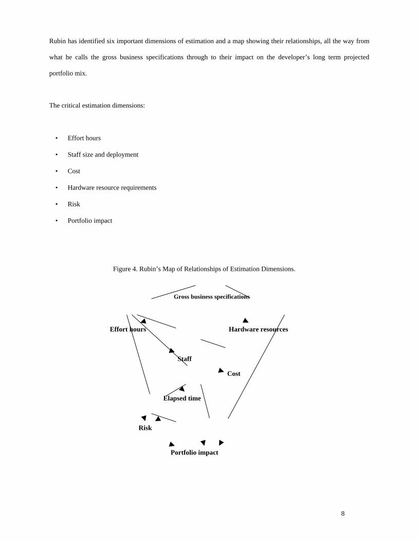
Rubin has identified six important dimensions of estimation and a map showing their relationships, all the way from
what he calls the gross business specifications through to their impact on the developer’s long term projected
portfolio mix.
The critical estimation dimensions:
• Effort hours
• Staff size and deployment
• Cost
• Hardware resource requirements
• Risk
• Portfolio impact
Figure 4. Rubin’s Map of Relationships of Estimation Dimensions.
Gross business specifications
Effort hours Hardware resources
Staff
Cost
Risk
Elapsed time
Portfolio impact

9
The basic premise of ESTIMACS is that the gross business specifications, or “project factors,” drive the estimate
dimensions. Rubin defines project factors as “aspects of the business functionality of the of the target system that are
well-defined early on, in a business sense, and are strongly linked to the estimate dimension.” Shown in table 1 are
the important project factors that inform each estimation dimension.
Table 1. Estimation Dimensions and Corresponding Project Factors.
Estimation Dimension Project Factors
Effort Hours Customer ComplexityCustomer GeographyDeveloper FamiliarityBusiness Function SizeTarget System SophisticationTarget System Complexity
Staff/Cost Effort HoursStaff ProductivitySkill Level DevelopmentRate at Each Skill Level
Hardware System CategoryGeneric System TypeOperating WindowTransaction Volume
Risk System SizeProject StructureTarget Technology
Portfolio Resource Needs of Concurrent ProjectsRelative Project Risks
The items in table 1 form the basis of the five submodels that comprise ESTIMACS. The submodels are designed to
be used sequentially, with outputs from one often serving as inputs to the next. Overall, the models support an
iterative approach to final estimate development, illustrated by the following list:
1. Data input/estimate evolution
2. Estimate summarization
3. Sensitivity analysis
4. Revision of step 1 inputs based upon results of step 3

10
The five ESTIMACS submodels in order of intended use:
System Development Effort Estimation: this model estimates development effort as total effort hours. It uses as
inputs the answers to twenty-five questions, eight related to the project organization and seventeen related to the
system structure itself. The broad project factors covered by these questions include developer knowledge of
application area, complexity of customer organization, the size, sophistication and complexity of the new system
being developed. Applying the answers to the twenty-five input questions to a customizable database of life-cycle
phases and work distribution, the model provides outputs of project effort in hours distributed by phase, and an
estimation bandwidth as a function of project complexity. It also outputs project size in function points to be used as
a basis for comparing relative sizes of systems.
Staffing and Cost Estimation: this model takes as input the effort hours distributed by phase derived in the previous
model. Other inputs include employee productivity and salaries by grade. It applies these inputs to an again
customizable work distribution life-cycle database. Outputs of the model include team size, staff distribution, and
cost all distributed by phase, peak load values and costs, and cumulative cost.
Hardware Configuration Estimates: this model sizes operational resource requirements of the hardware in the system
being developed. Inputs include application type, operating windows, and expected transaction volumes. Outputs are
estimates of required processor power by hour plus peak channel and storage requirements, based on a customizable
database of standard processors and device characteristics.
Risk Estimator: based mainly on a case study done by the Harvard Business School [Cash 1979], this model
estimates the risk of successfully completing the planned project. Inputs to this model include the answers to some
sixty questions, half of which are derived from use of the three previous submodels. These questions cover the
project factors of project size, structure and associated technology. Outputs include elements of project risk with
associated sensitivity analysis identifying the major contributors to those risks.
Portfolio Analyzer: a long range “big picture” planning tool, this last submodel estimates the simultaneous effects of
up to twenty projects over a ten year planning horizon. Inputs come from the Staffing & Cost Estimator and Risk

11
Estimator submodels. Scheduling projects via a Gantt chart, outputs include total staffing by skill level, cumulative
costs, monthly cash flows and relative risk. Comparisons between alternative portfolio or project mixes are possible.
The appeal of ESTIMACS lies in its ability to do estimates and sensitivity analyses of hardware as well as software,
and from its business-oriented planning approach.
2.5 SEER-SEM
SEER-SEM is a product offered by Galorath, Inc. of El Segundo, California (http://www.gaseer.com). This model is
based on the original Jensen model [Jensen 1983], and has been on the market some 15 years. During that time it has
evolved into a sophisticated tool supporting top-down and bottom-up estimation methodologies. Its modeling
equations are proprietary, but they take a parametric approach to estimation. The scope of the model is wide. It
covers all phases of the project life-cycle, from early specification through design, development, delivery and
maintenance. It handles a variety of environmental and application configurations, such as client-server, stand-alone,
distributed, graphics, etc. It models the most widely used development methods and languages. Development modes
covered include object oriented, reuse, COTS, spiral, waterfall, prototype and incremental development. Languages
covered are 3rd and 4th generation languages (C++, FORTRAN, COBOL, Ada, etc.), as well as application
generators. It allows staff capability, required design and process standards, and levels of acceptable development
risk to be input as constraints.
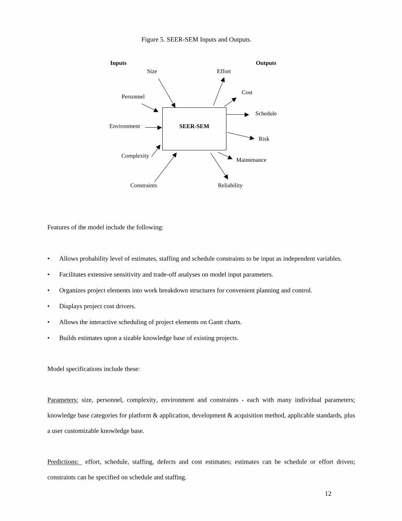
Figure 5 is adapted from a Galorath illustration and shows gross categories of model inputs and outputs, but each of
these represents dozens of specific input and output possibilities and parameters. The reports available from the
model covering all aspects of input and output summaries and analyses numbers in the hundreds.
12
Features of the model include the following:
• Allows probability level of estimates, staffing and schedule constraints to be input as independent variables.
• Facilitates extensive sensitivity and trade-off analyses on model input parameters.
• Organizes project elements into work breakdown structures for convenient planning and control.
• Displays project cost drivers.
• Allows the interactive scheduling of project elements on Gantt charts.
• Builds estimates upon a sizable knowledge base of existing projects.
Model specifications include these:
Parameters: size, personnel, complexity, environment and constraints - each with many individual parameters;
knowledge base categories for platform & application, development & acquisition method, applicable standards, plus
a user customizable knowledge base.
Predictions: effort, schedule, staffing, defects and cost estimates; estimates can be schedule or effort driven;
constraints can be specified on schedule and staffing.
Figure 5. SEER-SEM Inputs and Outputs.
Size
Personnel
Complexity
Environment
Constraints
Effort
Risk
Cost
Schedule
Maintenance
Reliability
Inputs Outputs
SEER-SEM

13
Risk Analysis: sensitivity analysis available on all least/likely/most values of output parameters; probability settings
for individual WBS elements adjustable, allowing for sorting of estimates by degree of WBS element criticality.
Sizing Methods: function points, both IFPUG sanctioned plus an augmented set; lines of code, both new and
existing.
Outputs and Interfaces: many capability metrics, plus hundreds of reports and charts; trade-off analyses with side-by-
side comparison of alternatives; integration with other Windows applications plus user customizable interfaces.
Aside from SEER-SEM, Galorath, Inc. offers a suite of many tools addressing hardware as well as software
concerns. One of particular interest to software estimators might be SEER-SEM, a tool designed to perform sizing of
software projects.
2.6 SELECT Estimator
SELECT Estimator by SELECT Software Tools is part of a suite of integrated products designed for components-
based development modeling. The company was founded in 1988 in the UK and has branch offices in California and
on the European continent. SELECT Estimator was released in 1998. It is designed for large scale distributed
systems development. It is object oriented, basing its estimates on business objects and components. It assumes an
incremental development life-cycle (but can be customized for other modes of development). The nature of its inputs
allows the model to be used at any stage of the software development life-cycle, most significantly even at the
feasibility stage when little detailed project information is known. In later stages, as more information is available, its
estimates become correspondingly more reliable.
The actual estimation technique is based upon ObjectMetrix developed by The Object Factory
(http://www.theobjectfactory.com). ObjectMetrix works by measuring the size of a project by counting and
classifying the software elements within a project. The project is defined in terms of business applications built out

14
of classes and supporting a set of use cases, plus infrastructure consisting of reusable components that provide a set
of services.
The ObjectMetrix techniques begin with a base metric of effort in person-days typically required to develop a given
project element. This effort assumes all the activities in a normal software development life-cycle are performed, but
assumes nothing about project characteristics or the technology involved that might qualify that effort estimate.
Pre-defined activity profiles covering planning, analysis, design, programming, testing, integration and review are
applied according to type of project element, which splits that base metric effort into effort by activity. (These
activity profiles are based upon project metric data collected and maintained by The Object Factory.)
The base effort is then adjusted by using “qualifiers” to add or subtract a percentage amount from each activity
estimate.
A “technology” factor addressing the impact of the given programming environment is then applied, this time
adding or subtracting a percentage amount from the “qualified” estimate.
Applying the qualifier and technology adjustments to the base metric effort for each project element produces an
overall estimate of effort in person-days, by activity. This total estimate represents the effort required by one person
of average skill level to complete the project.
Using the total one man effort estimate, schedule is then determined as a function of the number of developers—
input as an independent variable—then individual skill levels, the number of productive work days (excluding days
lost to meetings, illness, etc.) per month, plus a percentage contingency.
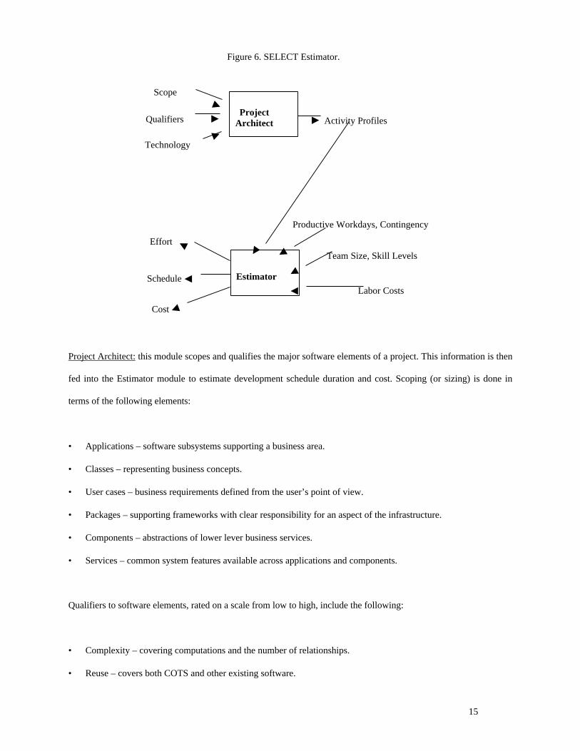
SELECT Estimator adapts the ObjectMetrix estimation technique by refining the Qualifier and Technology factors.
The tool itself consists of two modules, Project Architect and Estimator [SELECT 1998]. Figure 6 illustrates the
relationship between these modules.
15
Project Architect: this module scopes and qualifies the major software elements of a project. This information is then
fed into the Estimator module to estimate development schedule duration and cost. Scoping (or sizing) is done in
terms of the following elements:
• Applications – software subsystems supporting a business area.
• Classes – representing business concepts.
• User cases – business requirements defined from the user’s point of view.
• Packages – supporting frameworks with clear responsibility for an aspect of the infrastructure.
• Components – abstractions of lower lever business services.
• Services – common system features available across applications and components.
Qualifiers to software elements, rated on a scale from low to high, include the following:
• Complexity – covering computations and the number of relationships.
• Reuse – covers both COTS and other existing software.
Figure 6. SELECT Estimator.
Scope
Qualifiers
Technology
Activity Profiles
Labor Costs
Team Size, Skill Levels
Productive Workdays, Contingency
Effort
Schedule
Cost
ProjectArchitect
Estimator
16
• Genericity – whether the software needs to be built to be reusable.
• Technology – the choice of programming language.
Activity profiles are applied to the base metric effort adjusted by the scoping and qualifying factors to arrive at the
total effort estimate. Again, this is the effort required of one individual of average skill.
Estimator: this module uses the effort from the Project Architect to determine schedule duration and cost. Other
inputs include team size and skill levels (rated as novice, competent and expert); the number of productive workdays
per month and a contingency percentage; and the costs by skill level of the developers. The final outputs are total
effort in person-days, schedule duration in months, and total development cost.
2.7 COCOMO II
The COCOMO (COnstructive COst MOdel) cost and schedule estimation model was originally published in [Boehm
1981]. It became one of most popular parametric cost estimation models of the 1980s. But COCOMO '81 along with
its 1987 Ada update experienced difficulties in estimating the costs of software developed to new life-cycle
processes and capabilities. The COCOMO II research effort was started in 1994 at USC to address the issues on non-
sequential and rapid development process models, reengineering, reuse driven approaches, object oriented
approaches etc.
COCOMO II was initially published in the Annals of Software Engineering in 1995 [Boehm et al. 1995]. The model
has three submodels, Applications Composition, Early Design and Post-Architecture, which can be combined in
various ways to deal with the current and likely future software practices marketplace.
The Application Composition model is used to estimate effort and schedule on projects that use Integrated Computer
Aided Software Engineering tools for rapid application development. These projects are too diversified but
sufficiently simple to be rapidly composed from interoperable components. Typical components are GUI builders,
database or objects managers, middleware for distributed processing or transaction processing, etc. and domain-
specific components such as financial, medical or industrial process control packages. The Applications Composition

17
model is based on Object Points [Banker et al. 1994; Kauffman and Kumar 1993]. Object Points are a count of the
screens, reports and 3 GL language modules developed in the application. Each count is weighted by a three-level;
simple, medium, difficult; complexity factor. This estimating approach is commensurate with the level of information
available during the planning stages of Application Composition projects.
The Early Design model involves the exploration of alternative system architectures and concepts of operation.
Typically, not enough is known to make a detailed fine-grain estimate. This model is based on function points (or
lines of code when available) and a set of five scale factors and 7 effort multipliers.
The Post-Architecture model is used when top level design is complete and detailed information about the project is
available and as the name suggests, the software architecture is well defined and established. It
estimates for the entire development life-cycle and is a detailed extension of the Early-Design model. This model is
the closest in structure and formulation to the Intermediate COCOMO '81 and Ada COCOMO models. It uses
Source Lines of Code and/or Function Points for the sizing parameter, adjusted for reuse and breakage; a set of 17
effort multipliers and a set of 5 scale factors, that determine the economies/diseconomies of scale of the software
under development. The 5 scale factors replace the development modes in the COCOMO '81 model and refine the
exponent in the Ada COCOMO model.
The Post-Architecture Model has been calibrated to a database of 161 projects collected from Commercial,
Aerospace, Government and non-profit organizations using the Bayesian approach [Chulani et al. 1998b] discussed
further in section 7, “Composite Techniques”. The Early Design Model calibration is obtained by aggregating the
calibrated Effort Multipliers of the Post-Architecture Model as described in [USC-CSE 1997]. The Scale Factor
calibration is the same in both the models. Unfortunately, due to lack of data, the Application Composition model
has not yet been calibrated beyond an initial calibration to the [Kauffman and Kumar 1993] data.
A primary attraction of the COCOMO models is their fully-available internal equations and parameter values. Over a
dozen commercial COCOMO '81 implementations are available; one (Costar) also supports COCOMO II: for
details, see the COCOMO II website http://sunset.usc.edu/COCOMOII/suite.html.

18
2.8 Summary of Model Based Techniques
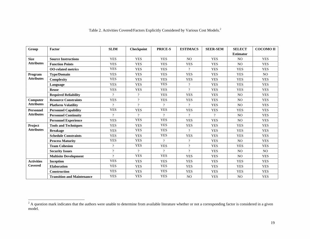
Table 2 summarizes the parameters used and activities covered by the models discussed. Overall, model based
techniques are good for budgeting, tradeoff analysis, planning and control, and investment analysis. As they are
calibrated to past experience, their primary difficulty is with unprecedented situations.
19
Table 2. Activities Covered/Factors Explicitly Considered by Various Cost Models.2
Group Factor SLIM Checkpoint PRICE-S ESTIMACS SEER-SEM SELECTEstimator
COCOMO II
Source Instructions YES YES YES NO YES NO YESFunction Points YES YES YES YES YES NO YES
SizeAttributes
OO-related metrics YES YES YES ? YES YES YESType/Domain YES YES YES YES YES YES NOComplexity YES YES YES YES YES YES YESLanguage YES YES YES ? YES YES YESReuse YES YES YES ? YES YES YES
ProgramAttributes
Required Reliability ? ? YES YES YES NO YESResource Constraints YES ? YES YES YES NO YESComputer
Attributes Platform Volatility ? ? ? ? YES NO YESPersonnel Capability YES YES YES YES YES YES YESPersonnel Continuity ? ? ? ? ? NO YES
PersonnelAttributes
Personnel Experience YES YES YES YES YES NO YESTools and Techniques YES YES YES YES YES YES YESBreakage YES YES YES ? YES YES YESSchedule Constraints YES YES YES YES YES YES YESProcess Maturity YES YES ? ? YES NO YESTeam Cohesion ? YES YES ? YES YES YESSecurity Issues ? ? ? ? YES NO NO
ProjectAttributes
Multisite Development ? YES YES YES YES NO YESInception YES YES YES YES YES YES YESElaboration YES YES YES YES YES YES YESConstruction YES YES YES YES YES YES YES
ActivitiesCovered
Transition and Maintenance YES YES YES NO YES NO YES
2 A question mark indicates that the authors were unable to determine from available literature whether or not a corresponding factor is considered in a givenmodel.

20
3. Expertise-Based Techniques
Expertise-based techniques are useful in the absence of quantified, empirical data. They capture the
knowledge and experience of practitioners seasoned within a domain of interest, providing estimates based
upon a synthesis of the known outcomes of all the past projects to which the expert is privy or in which he
or she participated. The obvious drawback to this method is that an estimate is only as good as the expert’s
opinion, and there is no way usually to test that opinion until it is too late to correct the damage if that
opinion proves wrong. Years of experience do not necessarily translate into high levels of competency.
Moreover, even the most highly competent of individuals will sometimes simply guess wrong. Two
techniques have been developed which capture expert judgement but that also take steps to mitigate the
possibility that the judgment of any one expert will be off. These are the Delphi technique and the Work
Breakdown Structure.
3.1 Delphi Technique
The Delphi technique [Helmer 1966] was developed at The Rand Corporation in the late 1940s originally as
a way of making predictions about future events - thus its name, recalling the divinations of the Greek oracle
of antiquity, located on the southern flank of Mt. Parnassos at Delphi. More recently, the technique has been
used as a means of guiding a group of informed individuals to a consensus of opinion on some issue.
Participants are asked to make some assessment regarding an issue, individually in a preliminary round,
without consulting the other participants in the exercise. The first round results are then collected, tabulated,
and then returned to each participant for a second round, during which the participants are again asked to
make an assessment regarding the same issue, but this time with knowledge of what the other participants
did in the first round. The second round usually results in a narrowing of the range in assessments by the
group, pointing to some reasonable middle ground regarding the issue of concern. The original Delphi
technique avoided group discussion; the Wideband Delphi technique [Boehm 1981] accommodated group
discussion between assessment rounds.

21
This is a useful technique for coming to some conclusion regarding an issue when the only information
available is based more on “expert opinion” than hard empirical data.
The authors have recently used the technique to estimate reasonable initial values for factors which appear in
two new software estimation models they are currently developing. Soliciting the opinions of a group of
experienced software development professionals, Abts and Boehm used the technique to estimate initial
parameter values for Effort Adjustment Factors (similar to factors shown in table 1) appearing in the glue
code effort estimation component of the COCOTS (COnstructive COTS) integration cost model [Abts 1997;
Abts et al. 1998].
Chulani and Boehm used the technique to estimate software defect introduction and removal rates during
various phases of the software development life-cycle. These factors appear in COQUALMO
(COnstructuve QUALity MOdel), which predicts the residual defect density in terms of number of
defects/unit of size[Chulani 1997]. Chulani and Boehm also used the Delphi approach to specify the prior
information required for the Bayesian calibration of COCOMO II [Chulani et 1998b].
3.2 Work Breakdown Structure (WBS)
Long a standard of engineering practice in the development of both hardware and software, the WBS is a
way of organizing project elements into a hierarchy that simplifies the tasks of budget estimation and
control. It helps determine just exactly what costs are being estimated. Moreover, if probabilities are
assigned to the costs associated with each individual element of the hierarchy, an overall expected value can
be determined from the bottom up for total project development cost [Baird 1989]. Expertise comes into
play with this method in the determination of the most useful specification of the components within the
structure and of those probabilities associated with each component.

22
Expertise-based methods are good for unprecedented projects and for participatory estimation, but
encounter the expertise-calibration problems discussed above and scalability problems for extensive
sensitivity analyses. WBS-based techniques are good for planning and control.
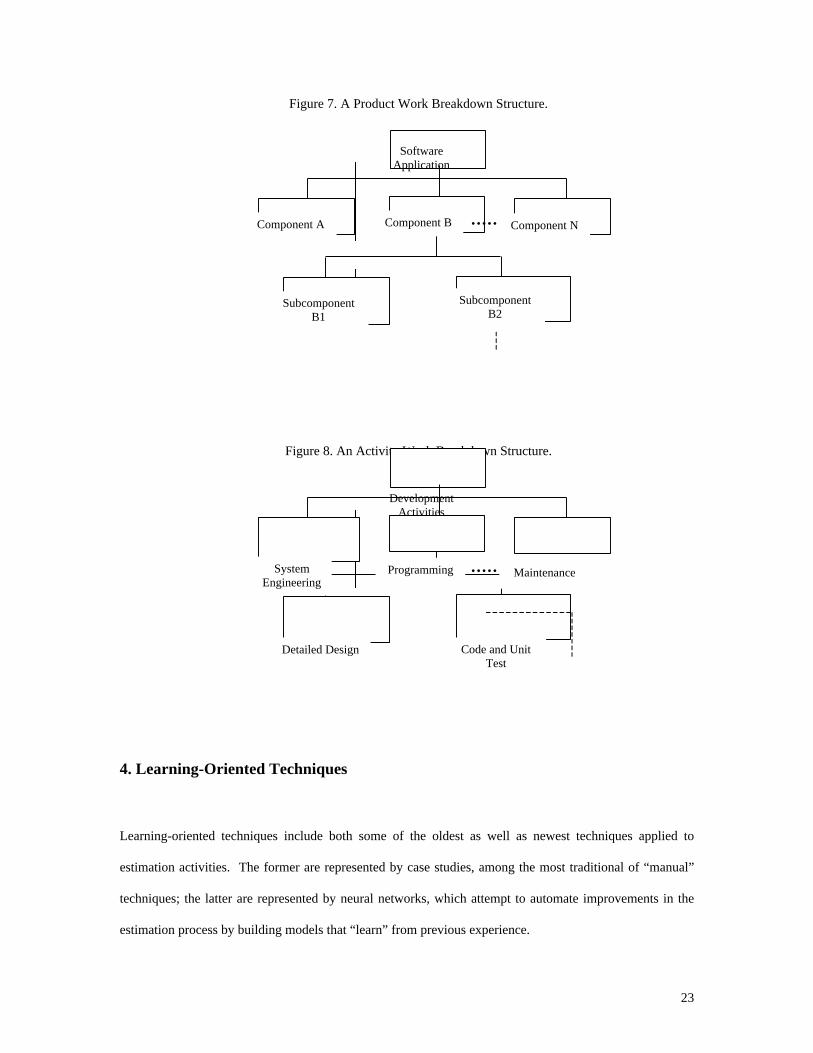
A software WBS actually consists of two hierarchies, one representing the software product itself, and the
other representing the activities needed to build that product [Boehm 1981]. The product hierarchy (figure
7) describes the fundamental structure of the software, showing how the various software components fit
into
the overall system. The activity hierarchy (figure 8) indicates the activities that may be associated with a
given software component.
Aside from helping with estimation, the other major use of the WBS is cost accounting and reporting. Each
element of the WBS can be assigned its own budget and cost control number, allowing staff to report the
amount of time they have spent working on any given project task or component, information that can then
be summarized for management budget control purposes.
Finally, if an organization consistently uses a standard WBS for all of its projects, over time it will accrue a
very valuable database reflecting its software cost distributions. This data can be used to develop a software
cost estimation model tailored to the organization’s own experience and practices.
23
4. Learning-Oriented Techniques
Learning-oriented techniques include both some of the oldest as well as newest techniques applied to
estimation activities. The former are represented by case studies, among the most traditional of “manual”
techniques; the latter are represented by neural networks, which attempt to automate improvements in the
estimation process by building models that “learn” from previous experience.
Figure 7. A Product Work Breakdown Structure.
SoftwareApplication
Component A Component B Component N
SubcomponentB1
SubcomponentB2
Figure 8. An Activity Work Breakdown Structure.
DevelopmentActivities
SystemEngineering
Programming Maintenance
Detailed Design Code and UnitTest

24
4.1 Case Studies
Case studies represent an inductive process, whereby estimators and planners try to learn useful general
lessons and estimation heuristics by extrapolation from specific examples. They examine in detail elaborate
studies describing the environmental conditions and constraints that obtained during the development of
previous software projects, the technical and managerial decisions that were made, and the final successes
or failures that resulted. They try to root out from these cases the underlying links between cause and effect
that can be applied in other contexts. Ideally they look for cases describing projects similar to the project
for which they will be attempting to develop estimates, applying the rule of analogy that says similar
projects are likely to be subject to similar costs and schedules. The source of case studies can be either
internal or external to the estimator’s own organization. “Homegrown” cases are likely to be more useful for
the purposes of estimation because they will reflect the specific engineering and business practices likely to
be applied to an organization’s projects in the future, but well-documented cases studies from other
organizations doing similar kinds of work can also prove very useful.
Shepperd and Schofield did a study comparing the use of analogy with prediction models based upon
stepwise regression analysis for nine datasets (a total of 275 projects), yielding higher accuracies for
estimation by analogy. They developed a five-step process for estimation by analogy:
§ identify the data or features to collect
§ agree data definitions and collections mechanisms
§ populate the case base
§ tune the estimation method
§ estimate the effort for a new project
For further details the reader is urged to read [Shepperd and Schofield 1997].

25
4.2 Neural Networks
According to Gray and McDonell [Gray and MacDonell 1996], neural networks is the most common
software estimation model-building technique used as an alternative to mean least squares regression. These
are estimation models that can be “trained” using historical data to produce ever better results by
automatically adjusting their algorithmic parameter values to reduce the delta between known actuals and
model predictions. Gray, et al., go on to describe the most common form of a neural network used in the
context of software estimation, a “backpropagation trained feed-forward” network (see figure 9).
The development of such a neural model is begun by first developing an appropriate layout of neurons, or
connections between network nodes. This includes defining the number of layers of neurons, the number of
neurons within each layer, and the manner in which they are all linked. The weighted estimating functions
between the nodes and the specific training algorithm to be used must also be determined. Once the network
has been built, the model must be trained by providing it with a set of historical project data inputs and the
corresponding known actual values for project schedule and/or cost. The model then iterates on its training
algorithm, automatically adjusting the parameters of its estimation functions until the model estimate and
the actual values are within some pre-specified delta. The specification of a delta value is important.
Without it, a model could theoretically become overtrained to the known historical data, adjusting its
estimation algorithms until it is very good at predicting results for the training data set, but weakening the
applicability of those estimation algorithms to a broader set of more general data.
Wittig [Wittig 1995] has reported accuracies of within 10% for a model of this type when used to estimate
software development effort, but caution must be exercised when using these models as they are often
subject to the same kinds of statistical problems with the training data as are the standard regression
techniques used to calibrate more traditional models. In particular, extremely large data sets are needed to
accurately train neural networks with intermediate structures of any complexity. Also, for negotiation and
sensitivity analysis, the neural networks provide little intuitive support for understanding the sensitivity

26
relationships between cost driver parameters and model results. They encounter similar difficulties for use
in planning and control.
5. Dynamics-Based Techniques
Dynamics-based techniques explicitly acknowledge that software project effort or cost factors change over
the duration of the system development; that is, they are dynamic rather than static over time. This is a
significant departure from the other techniques highlighted in this paper, which tend to rely on static models
and predictions based upon snapshots of a development situation at a particular moment in time. However,
factors like deadlines, staffing levels, design requirements, training needs, budget, etc., all fluctuate over the
course of development and cause corresponding fluctuations in the productivity of project personnel. This
in turn has consequences for the likelihood of a project coming in on schedule and within budget – usually
Figure 9. A Neural Network Estimation Model.
Data Inputs
Project Size
Complexity
Languages
Skill Levels
Estimation Algorithms
Model Output
EffortEstimate
Actuals
Training Algorithm

27
negative. The most prominent dynamic techniques are based upon the system dynamics approach to
modeling originated by Jay Forrester nearly forty years ago [Forrester 1961].
5.1 Dynamics-based Techniques
Dynamics-based techniques explicitly acknowledge that software project effort or cost factors change over
the duration of the system development; that is, they are dynamic rather than static over time. This is a
significant departure from the other techniques highlighted in this paper, which tend to rely on static models
and predictions based upon snapshots of a development situation at a particular moment in time. However,
factors like deadlines, staffing levels, design requirements, training needs, budget, etc., all fluctuate over the
course of development and cause corresponding fluctuations in the productivity of project personnel. This
in turn has consequences for the likelihood of a project coming in on schedule and within budget – usually
negative. The most prominent dynamic techniques are based upon the system dynamics approach to
modeling originated by Jay Forrester nearly forty years ago [Forrester 1961].
5.1 System Dynamics Approach
System dynamics is a continuous simulation modeling methodology whereby model results and behavior are
displayed as graphs of information that change over time. Models are represented as networks modified
with positive and negative feedback loops. Elements within the models are expressed as dynamically
changing levels or accumulations (the nodes), rates or flows between the levels (the lines connecting the
nodes), and information relative to the system that changes over time and dynamically affects the flow rates
between the levels (the feedback loops).
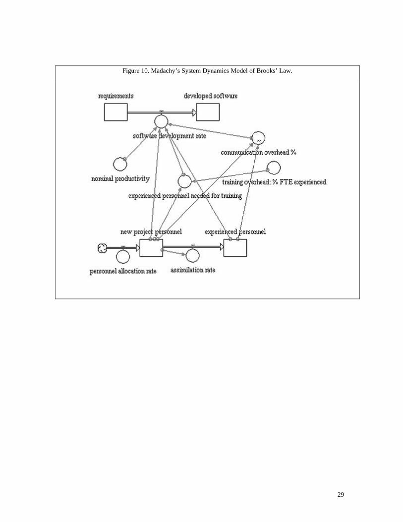
Figure 10 [Madachy 1999] shows an example of a system dynamics model demonstrating the famous
Brooks’ Law, which states that “adding manpower to a late software project makes it later” [Brooks 1975].
Brooks’ rationale is that not only does effort have to be reallocated to train the new people, but the
corresponding increase in communication and coordination overhead grows exponentially as people are
added.

28
Madachy’s dynamic model as shown in the figure illustrates Brooks’ concept based on the following
assumptions:
1) New people need to be trained by experienced people to improve their productivity.
2) Increasing staff on a project increases the coordination and communication overhead.
3) People who have been working on a project for a while are more productive than newly added people.
As can be seen in figure 10, the model shows two flow chains representing software development and
personnel. The software chain (seen at the top of the figure) begins with a level of requirements that need to
be converted into an accumulation of developed software. The rate at which this happens depends on the
number of trained personnel working on the project. The number of trained personnel in turn is a function
of the personnel flow chain (seen at the bottom of the figure). New people are assigned to the project
according to the personnel allocation rate, and then converted to experienced personnel according to the
assimilation rate. The other items shown in the figure (nominal productivity, communication overhead,
experienced personnel needed for training, and training overhead) are examples of auxiliary variables that
also affect the software development rate.
29
Figure 10. Madachy’s System Dynamics Model of Brooks’ Law.

30
Mathematically, system dynamics simulation models are represented by a set of first-order differential
equations [Madachy 1994]:
),()( pxftx' = Eq. 5.1
where
x = a vector describing the levels (states) in the model
p = a set of model parameters
f = a nonlinear vector function
t = time
Within the last ten years this technique has been applied successfully in the context of software engineering
estimation models. Abdel-Hamid has built models that will predict changes in project cost, staffing needs
and schedules over time, as long as the initial proper values of project development are available to the
estimator [Abdel-Hamid 1989a, 1989b, 1993; Abdel-Hamid and Madnick 1991]. He has also applied the
technique in the context of software reuse, demonstrating an interesting result. He found that there is an
initial beneficial relationship between the reuse of software components and project personnel productivity,
since less effort is being spent developing new code. However, over time this benefit diminishes if older
reuse components are retired and no replacement components have been written, thus forcing the
abandonment of the reuse strategy until enough new reusable components have been created, or unless they
can be acquired from an outside source [Abdel-Hamid and Madnick 1993].
31
More recently, Madachy used system dynamics to model an inspection-based software lifecycle process
[Madachy 1994]. He was able to show that performing software inspections during development slightly
increases programming effort, but decreases later effort and schedule during testing and integration.
Whether there is an overall savings in project effort resulting from that trade-off is a function of
development phase error injection rates, the level of effort required to fix errors found during testing, and
the efficiency of the inspection process. For typical industrial values of these parameters, the savings due to
inspections considerably outweigh the costs. Dynamics-based techniques are particularly good for planning
and control, but particularly difficult to calibrate.
6. Regression-Based Techniques
Regression-based techniques are the most popular ways of building models. These techniques are used in
conjunction with model-based techniques and include “Standard” regression, “Robust” regression, etc.
6.1 “Standard” Regression – Ordinary Least Squares (OLS) method
“Standard” regression refers to the classical statistical approach of general linear regression modeling using
least squares. It is based on the Ordinary Least Squares (OLS) method discussed in many books such as
[Judge et al. 1993; Weisberg 1985]. The reasons for its popularity include ease of use and simplicity. It is
available as an option in several commercial statistical packages such as Minitab, SPlus, SPSS, etc.
A model using the OLS method can be written as
y x B x et t k tk t= + + + +β β1 2 2 ... Eq. 6.1

32
where xt2 … xtk are predictor (or regressor) variables for the tth observation, β2 ... βκ are response
coefficients, β1 is an intercept parameter and yt is the response variable for the tth observation. The error
term, et is a random variable with a probability distribution (typically normal). The OLS method operates by
estimating the response coefficients and the intercept parameter by minimizing the least squares error term
ri2 where ri
is the difference between the observed response and the model predicted response for the ith
observation. Thus all observations have an equivalent influence on the model equation. Hence, if there is an
outlier in the observations then it will have an undesirable impact on the model.
The OLS method is well-suited when
(i) a lot of data are available. This indicates that there are many degrees of freedom available and the
number of observations is many more than the number of variables to be predicted. Collecting data has
been one of the biggest challenges in this field due to lack of funding by higher management, co-
existence of several development processes, lack of proper interpretation of the process, etc.
(ii) no data items are missing. Data with missing information could be reported when there is limited time
and budget for the data collection activity; or due to lack of understanding of the data being reported.
(iii) there are no outliers. Extreme cases are very often reported in software engineering data due to
misunderstandings or lack of precision in the data collection process, or due to different “development”
processes.
(iv) the predictor variables are not correlated. Most of the existing software estimation models have
parameters that are correlated to each other. This violates the assumption of the OLS approach.
(v) the predictor variables have an easy interpretation when used in the model. This is very difficult to
achieve because it is not easy to make valid assumptions about the form of the functional relationships
between predictors and their distributions.
(vi) the regressors are either all continuous (e.g. Database size) or all discrete variables (ISO 9000
certification or not). Several statistical techniques exist to address each of these kind of variables but
not both in the same model.

33
Each of the above is a challenge in modeling software engineering data sets to develop a robust, easy-to-
understand, constructive cost estimation model.
A variation of the above method was used to calibrate the 1997 version of COCOMO II. Multiple
regression was used to estimate the b coefficients associated with the 5 scale factors and 17 effort
multipliers. Some of the estimates produced by this approach gave counter intuitive results. For example,
the data analysis indicated that developing software to be reused in multiple situations was cheaper than
developing it to be used in a single situation: hardly a credible predictor for a practical cost estimation
model. For the 1997 version of COCOMO II, a pragmatic 10% weighted average approach was used.
COCOMO II.1997 ended up with a 0.9 weight for the expert data and a 0.1 weight for the regression data.
This gave moderately good results for an interim COCOMO II model, with no cost drivers operating in non-
credible ways.
6.2 “Robust” Regression
Robust Regression is an improvement over the standard OLS approach. It alleviates the common problem
of outliers in observed software engineering data. Software project data usually have a lot of outliers due to
disagreement on the definitions of software metrics, coexistence of several software development processes
and the availability of qualitative versus quantitative data.
There are several statistical techniques that fall in the category of ‘Robust” Regression. One of the
techniques is based on Least Median Squares method and is very similar to the OLS method described
above. The only difference is that this technique reduces the median of all the ri2 .
Another approach that can be classified as “Robust” regression is a technique that uses the datapoints lying
within two (or three) standard deviations of the mean response variable. This method automatically gets rid
34
of outliers and can be used only when there is a sufficient number of observations, so as not to have a
significant impact on the degrees of freedom of the model. Although this technique has the flaw of
eliminating outliers without direct reasoning, it is still very useful for developing software estimation
models with few regressor variables due to lack of complete project data.
Most existing parametric cost models (COCOMO II, SLIM, Checkpoint etc.) use some form of regression-
based techniques due to their simplicity and wide acceptance.
7. Composite Techniques
As discussed above there are many pros and cons of using each of the existing techniques for cost
estimation. Composite techniques incorporate a combination of two or more techniques to formulate the
most appropriate functional form for estimation.
7.1 Bayesian Approach
An attractive estimating approach that has been used for the development of the COCOMO II model is
Bayesian analysis [Chulani et al. 1998].
Bayesian analysis is a mode of inductive reasoning that has been used in many scientific disciplines. A
distinctive feature of the Bayesian approach is that it permits the investigator to use both sample (data) and
prior (expert-judgement) information in a logically consistent manner in making inferences. This is done by
using Bayes’ theorem to produce a ‘post-data’ or posterior distribution for the model parameters. Using
Bayes’ theorem, prior (or initial) values are transformed to post-data views. This transformation can be
viewed as a learning process. The posterior distribution is determined by the variances of the prior and
sample information. If the variance of the prior information is smaller than the variance of the sampling
information, then a higher weight is assigned to the prior information. On the other hand, if the variance of

35
the sample information is smaller than the variance of the prior information, then a higher weight is
assigned to the sample information causing the posterior estimate to be closer to the sample information.
The Bayesian approach provides a formal process by which a-priori expert-judgement can be combined
with sampling information (data) to produce a robust a-posteriori model. Using Bayes’ theorem, we can
combine our two information sources as follows:
f Yf Y f
f Y( | )
( | ) ( )( )
ββ β
= Eq. 7.1
where ß is the vector of parameters in which we are interested and Y is the vector of sample observations
from the joint density function f Y( | )β . In equation 7.1, f Y( | )β is the posterior density
function for ß summarizing all the information about ß, f Y( | )β is the sample information and is
algebraically equivalent to the likelihood function for ß, and f ( )β is the prior information summarizing
the expert-judgement information about ß. Equation 7.1 can be rewritten as
f Y l Y f( | ) ( | ) ( )β β β∝ Eq. 7.2
In words, equation 7.2 means
Posterior ∝ Sample * Prior
In the Bayesian analysis context, the “prior” probabilities are the simple “unconditional” probabilities
associated with the sample information, while the “posterior” probabilities are the “conditional”
probabilities given knowledge of sample and prior information.

36
The Bayesian approach makes use of prior information that is not part of the sample data by providing an
optimal combination of the two sources of information. As described in many books on Bayesian analysis
[Leamer 1978; Box 1973], the posterior mean, b**, and variance, Var(b**), are defined as
bs
X X Hs
X Xb H b** * * *[ ' ] '= + × +
−1 12
12 Eq. 7.3
and
Var bs
X X H( ) '** *= +
−12
1
Eq. 7.4
where X is the matrix of predictor variables, s is the variance of the residual for the sample data; and H*
and b* are the precision (inverse of variance) and mean of the prior information respectively.
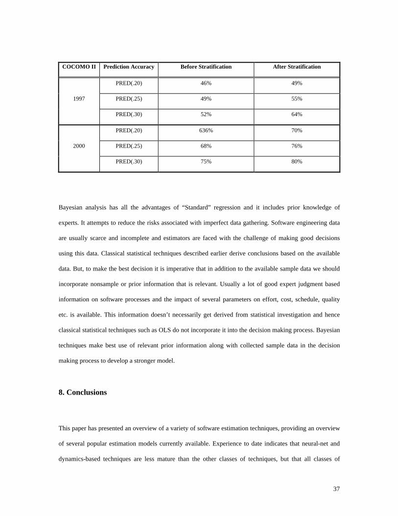
The Bayesian approach described above has been used in the most recent calibration of COCOMO II over a
database currently consisting of 161 project data points. The a-posteriori COCOMO II.2000 calibration
gives predictions that are within 30% of the actuals 75% of the time, which is a significant improvement
over the COCOMO II.1997 calibration which gave predictions within 30% of the actuals 52% of the time as
shown in table 3. (The 1997 calibration was not performed using Bayesian analysis; rather, a 10% weighted
linear combination of expert prior vs. sample information was applied [Clark et al. 1998].) If the model’s
multiplicative coefficient is calibrated to each of the major sources of project data, i.e., “stratified” by data
source, the resulting model produces estimates within 30% of the actuals 80% of the time. It is therefore
recommended that organizations using the model calibrate it using their own data to increase model
accuracy and produce a local optimum estimate for similar type projects. From table 3 it is clear that the
predictive accuracy of the COCOMO II.2000 Bayesian model is better than the predictive accuracy of the
COCOMO II.1997 weighted linear model illustrating the advantages of using Composite techniques.
Table 3. Prediction Accuracy of COCOMO II.1997 vs. COCOMO II.2000.
37
COCOMO II Prediction Accuracy Before Stratification After Stratification
PRED(.20) 46% 49%
1997 PRED(.25) 49% 55%
PRED(.30) 52% 64%
PRED(.20) 636% 70%
2000 PRED(.25) 68% 76%
PRED(.30) 75% 80%
Bayesian analysis has all the advantages of “Standard” regression and it includes prior knowledge of
experts. It attempts to reduce the risks associated with imperfect data gathering. Software engineering data
are usually scarce and incomplete and estimators are faced with the challenge of making good decisions
using this data. Classical statistical techniques described earlier derive conclusions based on the available
data. But, to make the best decision it is imperative that in addition to the available sample data we should
incorporate nonsample or prior information that is relevant. Usually a lot of good expert judgment based
information on software processes and the impact of several parameters on effort, cost, schedule, quality
etc. is available. This information doesn’t necessarily get derived from statistical investigation and hence
classical statistical techniques such as OLS do not incorporate it into the decision making process. Bayesian
techniques make best use of relevant prior information along with collected sample data in the decision
making process to develop a stronger model.
8. Conclusions
This paper has presented an overview of a variety of software estimation techniques, providing an overview
of several popular estimation models currently available. Experience to date indicates that neural-net and
dynamics-based techniques are less mature than the other classes of techniques, but that all classes of

38
techniques are challenged by the rapid pace of change in software technology. The important lesson to take
from this paper is that no one method or model should be preferred over all others. The key to arriving at
sound estimates is to use a variety of methods and tools and then investigating the reasons why the estimates
provided by one might differ significantly from those provided by another. If the practitioner can explain
such differences to a reasonable level of satisfaction, then it is likely that he or she has a good grasp of the
factors which are driving the costs of the project at hand; and thus will be better equipped to support the
necessary project planning and control functions performed by management.
9. References
Abdel-Hamid, T. (1989a), “The Dynamics of Software Project Staffing: A System Dynamics-based
Simulation Approach,” Abdel-Hamid, T., IEEE Transactions on Software Engineering, February 1989.
Abdel-Hamid, T. (1989b), “Lessons Learned from Modeling the Dynamics of Software Development,”
Abdel-Hamid, T., Communications of the ACM, December 1989.
Abdel-Hamid, T. and Madnick, S. (1991), Software Project Dynamics, Abdel-Hamid, T. and Madnick, S.,
Prentice-Hall, 1991.
Abdel-Hamid, T. (1993), “Adapting, Correcting, and Perfecting Software Estimates: a Maintenance
Metaphor,” Abdel-Hamid, T., IEEE Computer, March 1993.
Abdel-Hamid, T. and Madnick, S. (1993), “Modeling the Dynamics of Software Reuse: an Integrating
System Dynamics Perspective,” Abdel-Hamid, T. and Madnick, S., presentation to the 6th Annual
Workshop on Reuse, Owego, NY, November 1993.

39
Abts, C. (1997), “COTS Software Integration Modeling Study,” Abts, C., Report prepared for USAF
Electronics System Center, Contract No. F30602-94-C-1095, University of Southern California, 1997.
Abts, C., Bailey, B. and Boehm, B (1998), “COCOTS Software Integration Cost Model: An Overview,”
Abts, C., Bailey, B. and Boehm, B., Proceedings of the California Software Symposium, 1998.
Albrecht, A. (1979), “Measuring Application Development Productivity,” Albrecht, A., Proceedings of the
Joint SHARE/GUIDE/IBM Application Development Symposium, Oct. 1979, pp. 83-92.
Baird, B. (1989), Managerial Decisions Under Uncertainty, Baird, B., John Wiley & Sons, 1989.
Banker, R., Kauffman, R. and Kumar, R. (1994), An Empirical Test of Object-Based Output Measurement
Metrics in a Computer Aided Software Engineering (CASE) Environment,” Banker, R., Kauffman, R. and
Kumar, R., Journal of Management Information System, 1994.
Boehm, B. (1981), Software Engineering Economics, Boehm, B., Prentice Hall, 1981.
Boehm, B., Clark, B., Horowitz, E., Westland, C., Madachy, R., Selby, R. (1995), “Cost Models for Future
Software Life-cycle Processes: COCOMO 2.0,” Boehm, B., Clark, B., Horowitz, E., Westland, C.,
Madachy, R., Selby, R., Annals of Software Engineering Special Volume on Software Process and Product
Measurement, J.D. Arthur and S.M. Henry (Eds.), J.C. Baltzer AG, Science Publishers, Amsterdam, The
Netherlands, Vol 1, 1995, pp. 45 - 60.
Box, G. and Tiao, G. (1973), Bayesian Inference in Statistical Analysis, Box, G. and Tiao, G., Addison
Wesley, 1973.

40
Briand, L., Basili V. and Thomas, W. (1992), “A Pattern Recognition Approach for Software Engineering
Data Analysis,” Briand, L., Basili V. and Thomas, W., IEEE Transactions on Software Engineering, Vol.
18, No. 11, November 1992.
Brooks (1975) The Mythical Man-Month, Brooks, F., Addison-Wesley, Reading, MA, 1975.
Cash, J. (1979), “Dallas Tire Case,” J. I. Cash, Harvard Business School, 1979.
Chidamber, S. and Kemerer, C. (1994), “A Metrics Suite for Object Oriented Design,” Chidamber, S. and
Kemerer, C., CISR WP No. 249 and Sloan WP No. 3524-93, Center for Information Systems Research,
Sloan School of Management, Massachusetts Institute of Technology.
Chulani, S. (1997), “Modeling Defect Introduction,” Chulani, S., California Software Symposium, Nov
1997.
Chulani, S. (1998), “Incorporating Bayesian Analysis to Improve the Accuracy of COCOMO II and Its
Quality Model Extension,” Chulani, S., Ph.D. Qualifying Exam Report, University of Southern California,
Feb 1998.
Chulani, S., Boehm, B. and Steece, B. (1998b), “Calibrating Software Cost Models Using Bayesian
Analysis,” Chulani S., Boehm, B. and Steece, B., Technical Report, USC-CSE-98-508, Jun 1998. To
appear in IEEE Transactions on Software Engineering, Special Issue on Empirical Methods in Software
Engineering.
Clark, B., Chulani, S. and Boehm, B. (1998), “Calibrating the COCOMO II Post Architecture Model,”
Clark, B., Chulani, S. and Boehm, B., International Conference on Software Engineering, Apr. 1998.

41
Forrester, J. (1961) – Industrial Dynamics, Forrester, J., MIT Press, Cambridge, MA, 1961.
Gray, A. and MacDonell, S. (1996) – “A Comparison of Techniques for Developing Predictive Models of
Software Metrics,” Gray, A and MacDonell, S., Information and Software Technology 39, 1997.
Helmer, O. (1966), Social Technology, Helmer, O., Basic Books, NY, 1966.
Henderson-Sellers, B. (1996), Object Oriented Metrics -Measures of Complexity, Henderson-Sellers, B.,
Prentice Hall, Upper Saddle River, NJ, 1996.
Jensen R. (1983) – “An Improved Macrolevel Software Development Resource Estimation Model,” Jensen
R., Proceedings 5th ISPA Conference, April 1983, pp. 88-92.
Jones, C. (1997), Applied Software Measurement, Jones, C., 1997, McGraw Hill.
Judge, G., Griffiths, W. and Hill, C. (1993), Learning and Practicing Econometrics, Judge, G., Griffiths,
W. and Hill, C., Wiley, 1993.
Kauffman, R. and Kumar, R. (1993), “Modeling Estimation Expertise in Object Based ICASE
Environments,” Kauffman, R., and Kumar, R., Stern School of Business Report, New York University,
January 1993.
Khoshgoftaar T., Pandya A. and Lanning, D. (1995), “Application of Neural Networks for predicting
program faults,” Khoshgoftaar T., Pandya A. and Lanning, D., Annals of Software Engineering, Vol. 1,
1995.

42
Leamer, E. (1978), Specification Searches, Ad hoc Inference with Nonexperimental Data. Leamer, E.,
Wiley Series, 1978.
Madachy, R. (1994), “A Software Project Dynamics Model for Process Cost, Schedule and Risk
Assessment,” Ph.D. dissertation, Madachy, R., University of Southern California, 1994.
Madachy, R. (1999), CS577a class notes, Madachy, R., University of Southern California, 1999.
Minkiewicz, A. (1998), “Measuring Object Oriented Software with Predictive Object Points,” Minkeiwicz,
A., PRICE Systems, 1998.
Nelson, E. (1966) – “Management Handbook for the Estimation of Computer Programming Costs,” Nelson,
E., Systems Development Corporation, Oct. 1966.
Park R. (1988), “The Central Equations of the PRICE Software Cost Model,” Park R., 4th COCOMO Users’
Group Meeting, November 1988.
Putnam, L. and Myers, W. (1992), Measures for Excellence, Putnam, L. and Myers, W., 1992, Yourdon
Press Computing Series.
Rubin, H. (1983), “ESTIMACS,” Rubin, H., IEEE, 1983.
SELECT (1998), “Estimation for Component-based Development Using SELECT Estimator,” SELECT
Software Tools, 1998. Website: http://www.selectst.com
43
Shepperd, M. and Schofield, M. (1997), “Estimating Software Project Effort Using Analogies,” Shepperd,
M. and Schofield, M., IEEE Transactions on Software Engineering, Nov 1997, Vol. 23, No. 12.
Symons (1991), “Software Sizing and Estimating – Mark II FPA,” Symons C., John Wiley and Sons, U.K.,
ISBN 0-471-92985-9, 1991.
USC-CSE (1997), “COCOMO II Model Definition Manual,” Center for Software Engineering, Computer
Science Department, University of Southern California, Los Angeles, CA. 90007, website:
http://sunset.usc.edu/COCOMOII/cocomo.html, 1997.
Weisberg, S. (1985), Applied Linear Regression, Weisberg, S., 2nd Ed., John Wiley and Sons, New York,
N.Y., 1985.
Wittig, G (1995) – “Estimating Software Development Effort with Connectionist Models,” Wittig, G.,
Working Paper Series 33/95, Monash University, 1995.
10. Acknowledgements
This research is sponsored by the Affiliates of the USC Center for Software Engineering: Aerospace, Air
Force Cost Analysis Agency, Allied Signal, AT&T, Bellcore, EDS, Raytheon E-Systems, GDE Systems,
Hughes, IDA, JPL, Litton, Lockheed Martin, Loral, MCC, MDAC, Motorola, Northrop Grumman,
Rational, Rockwell, SAIC, SEI, SPC, Sun, TI, TRW, USAF Rome Labs, US Army Research Labs and
Xerox.
Special thanks to the model and tool vendors who provided the authors with the information required to
perform this study.

Filename: ASEpaper_incorporating_reviewer_comments.docDirectory: C:\Program Files\Qualcomm\Eudora Pro\AttachTemplate: C:\Program Files\Microsoft Office\Office\Normal.dotTitle: 2Subject:Author: Sunita DevinaniKeywords:Comments:Creation Date: 03/23/00 11:25 AMChange Number: 2Last Saved On: 03/23/00 11:25 AMLast Saved By: IBM UserTotal Editing Time: 3 MinutesLast Printed On: 04/11/00 10:33 AMAs of Last Complete Printing
Number of Pages: 45Number of Words: 10,263 (approx.)Number of Characters: 57,473 (approx.)
Related Documents