SoftPOSIT: Simultaneous Pose and Correspondence …ramani/pubs/softposit.pdfSoftPOSIT: Simultaneous Pose and Correspondence Determination PHILIP DAVID University of Maryland Institute

International Journal of Computer Vision 59(3), 259–284, 2004c© 2004 Kluwer Academic Publishers. Manufactured in The Netherlands.

SoftPOSIT: Simultaneous Pose and Correspondence Determination

PHILIP DAVIDUniversity of Maryland Institute for Advanced Computer Studies, College Park, MD 20742, USA;

Army Research Laboratory, 2800 Powder Mill Road, Adelphi, MD 20783-1197, USA

DANIEL DEMENTHON, RAMANI DURAISWAMI AND HANAN SAMETUniversity of Maryland Institute for Advanced Computer Studies, College Park, MD 20742, USA

Received November 21, 2002; Revised September 3, 2003; Accepted November 18, 2003

Abstract. The problem of pose estimation arises in many areas of computer vision, including object recognition,object tracking, site inspection and updating, and autonomous navigation when scene models are available. Wepresent a new algorithm, called SoftPOSIT, for determining the pose of a 3D object from a single 2D image whencorrespondences between object points and image points are not known. The algorithm combines the iterativesoftassign algorithm (Gold and Rangarajan, 1996; Gold et al., 1998) for computing correspondences and theiterative POSIT algorithm (DeMenthon and Davis, 1995) for computing object pose under a full-perspective cameramodel. Our algorithm, unlike most previous algorithms for pose determination, does not have to hypothesize smallsets of matches and then verify the remaining image points. Instead, all possible matches are treated identicallythroughout the search for an optimal pose. The performance of the algorithm is extensively evaluated in MonteCarlo simulations on synthetic data under a variety of levels of clutter, occlusion, and image noise. These testsshow that the algorithm performs well in a variety of difficult scenarios, and empirical evidence suggests that thealgorithm has an asymptotic run-time complexity that is better than previous methods by a factor of the numberof image points. The algorithm is being applied to a number of practical autonomous vehicle navigation problemsincluding the registration of 3D architectural models of a city to images, and the docking of small robots onto largerrobots.

Keywords: object recognition, autonomous navigation, POSIT, softassign

1. Introduction

This paper presents an algorithm for solving the model-to-image registration problem, which is the task of de-termining the position and orientation (the pose) of athree-dimensional object with respect to a camera co-ordinate system, given a model of the object consistingof 3D reference points and a single 2D image of thesepoints. We assume that no additional information isavailable with which to constrain the pose of the objector to constrain the correspondence of object features toimage features. This is also known as the simultaneouspose and correspondence problem.

Automatic registration of 3D models to images is animportant problem. Applications include object recog-nition, object tracking, site inspection and updating,and autonomous navigation when scene models areavailable. It is a difficult problem because it comprisestwo coupled problems, the correspondence problemand the pose problem, each easy to solve only if theother has been solved first:

1. Solving the pose (or exterior orientation) problemconsists of finding the rotation and translation ofthe object with respect to the camera coordinate sys-tem. Given matching object and image features, one

260 David et al.

can easily determine the pose that best aligns thosematches. For three to five matches, the pose canbe found in closed form by solving sets of polyno-mial equations (Fischler and Bolles, 1981; Haralicket al., 1991; Horaud et al., 1989; Yuan, 1989). Forsix or more matches, linear and approximate non-linear methods are generally used (DeMenthon andDavis, 1995; Fiore, 2001; Hartley and Zisserman,2000; Horn, 1986; Lu et al., 2000).

2. Solving the correspondence problem consists offinding matching object and image features. If theobject pose is known, one can relatively easily de-termine the matching features. Projecting the ob-ject in the known pose into the original image, onecan identify matches among the object features thatproject sufficiently close to an image feature. Thisapproach is typically used for pose verification,which attempts to determine how good a hypoth-esized pose is (Grimson and Huttenlocher, 1991).

The classic approach to solving these coupled prob-lems is the hypothesize-and-test approach (Grimson,1990). In this approach, a small set of object feature toimage feature correspondences are first hypothesized.Based on these correspondences, the pose of the ob-ject is computed. Using this pose, the object pointsare back-projected into the image. If the original andback-projected images are sufficiently similar, then thepose is accepted; otherwise, a new hypothesis is formedand this process is repeated. Perhaps the best knownexample of this approach is the RANSAC algorithm(Fischler and Bolles, 1981) for the case that no infor-mation is available to constrain the correspondencesof object points to image points. When three corre-spondences are used to determine a pose, a high prob-ability of success can be achieved by the RANSACalgorithm in O(M N 3 log N ) time when there are Mobject points and N image points (see Appendix A fordetails).

The problem addressed here is one that is encoun-tered when taking a model-based approach to the objectrecognition problem, and as such has received consid-erable attention. (The other main approach to objectrecognition is the appearance-based approach (Muraseand Nayar, 1995) in which multiple views of the objectare compared to the image. However, since 3D modelsare not used, this approach doesn’t provide accurate ob-ject pose.) Many investigators (e.g., Cass, 1994, 1998;Ely et al., 1995; Jacobs, 1992; Lamdan and Wolfson,1988; Procter and Illingworth, 1997) approximate the

nonlinear perspective projection via linear affine ap-proximations. This is accurate when the relative depthsof object features are small compared to the distanceof the object from the camera. Among the pioneer con-tributions were Baird’s tree-pruning method (Baird,1985), with exponential time complexity for unequalpoint sets, and Ullman’s alignment method (Ullman,1989) with time complexity O(N 4 M3 log M).

The geometric hashing method (Lamdan andWolfson, 1988) determines an object’s identity andpose using a hashing metric computed from a set ofimage features. Because the hashing metric must beinvariant to camera viewpoint, and because there areno view-invariant image features for general 3D pointsets (for either perspective or affine cameras) (Burnset al., 1993), this method can only be applied to planarscenes.

In DeMenthon and Davis (1993), we proposed an ap-proach using binary search by bisection of pose boxesin two 4D spaces, extending the research of Baird(1985), Cass (1992), and Breuel (1992) on affine trans-forms, but it had high-order complexity. The approachtaken by Jurie (1999) was inspired by our work andbelongs to the same family of methods. An initial vol-ume of pose space is guessed, and all of the correspon-dences compatible with this volume are first taken intoaccount. Then the pose volume is recursively reduceduntil it can be viewed as a single pose. As a Gaussian er-ror model is used, boxes of pose space are pruned notby counting the number of correspondences that arecompatible with the box as in DeMenthon and Davis(1993), but on the basis of the probability of having anobject model in the image within the range of posesdefined by the box.

Among the researchers who have addressed the fullperspective problem, Wunsch and Hirzinger (1996) for-malize the abstract problem in a way similar to theapproach advocated here as the optimization of an ob-jective function combining correspondence and poseconstraints. However, the correspondence constraintsare not represented analytically. Instead, each objectfeature is explicitly matched to the closest lines of sightof the image features. The closest 3D points on the linesof sight are found for each object feature, and the posethat brings the object features closest to these 3D pointsis selected; this allows an easier 3D to 3D pose problemto be solved. The process is repeated until a minimumof the objective function is reached.

The object recognition approach of Beis andLowe (1999) uses view-variant 2D image features to

SoftPOSIT: Simultaneous Pose and Correspondence Determination 261

index 3D object models. Off-line training is performedto learn 2D feature groupings associated with largenumbers of views of the objects. Then, the on-linerecognition stage uses new feature groupings to indexinto a database of learned object-to-image correspon-dence hypotheses, and these hypotheses are used forpose estimation and verification.

The pose clustering approach to model-to-image reg-istration is similar to the classic hypothesize-and-testapproach. Instead of testing each hypothesis as it isgenerated, all hypotheses are generated and clusteredin a pose space before any back-projection and testingtakes place. This later step is performed only on posesassociated with high-probability clusters. The ideais that hypotheses including only correct correspon-dences should form larger clusters in pose space thanhypotheses that include incorrect correspondences.Olson (1997) gives a randomized algorithm for poseclustering whose time complexity is O(M N 3).

The method of Beveridge and Riseman (1992, 1995)is also related to our approach. Random-start localsearch is combined with a hybrid pose estimation al-gorithm employing both full-perspective and weak-perspective camera models. A steepest descent searchin the space of object-to-image line segment correspon-dences is performed. A weak-perspective pose algo-rithm is used to rank neighboring points in this searchspace, and a full-perspective pose algorithm is used toupdate the object’s pose after making a move to a newset of correspondences. The time complexity of this al-gorithm was empirically determined to be O(M2 N 2).

When there are M object points and N image points,the dimension of the solution space for this problem isM +6 since there are M correspondence variables and6 pose variables. Each correspondence variable has thedomain {1, 2, . . . , N , ∅} representing a match of an ob-ject point to one of the N image points or to no imagepoint (represented by ∅), and each pose variable hasa continuous domain determined by the allowed rangeof object translations and rotations. Most algorithmsdon’t explicitly search this M + 6-dimensional space,but instead assume that pose is determined by cor-respondences or that correspondences are determinedby pose, and so search either an M-dimensional or a6-dimensional space. The SoftPOSIT approach is dif-ferent in that its search alternates between these twospaces.

The SoftPOSIT approach to solving the model-to-image registration problem applies the formalismproposed by Gold, Rangarajan and others (Gold and

Rangarajan, 1996; Gold et al., 1998) when they solvedthe correspondence and pose problem in matching twoimages or two 3D objects. We extend it to the moredifficult problem of registration between a 3D objectand its perspective image, which they did not address.The SoftPOSIT algorithm integrates an iterative posetechnique called POSIT (Pose from Orthographyand Scaling with ITerations) (DeMenthon and Davis,1995), and an iterative correspondence assignmenttechnique called softassign (Gold and Rangarajan,1996; Gold et al., 1998) into a single iteration loop.A global objective function is defined that capturesthe nature of the problem in terms of both pose andcorrespondence and combines the formalisms of bothiterative techniques. The correspondence and thepose are determined simultaneously by applying adeterministic annealing schedule and by minimizingthis global objective function at each iteration step.

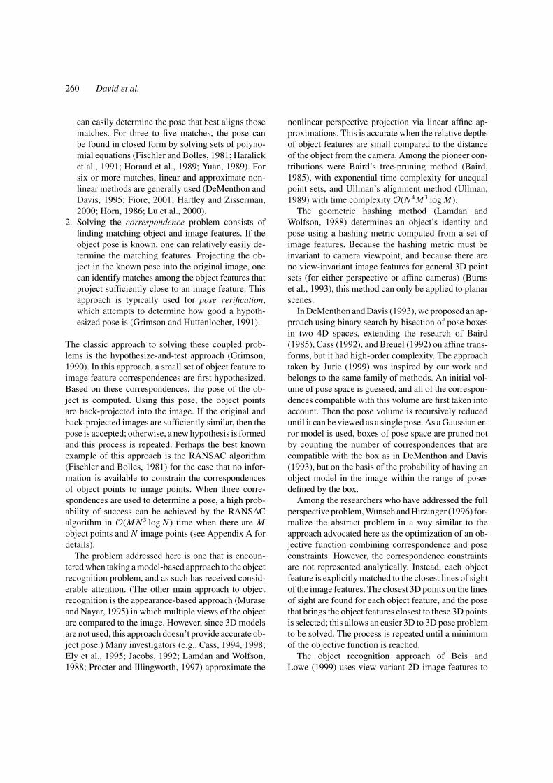
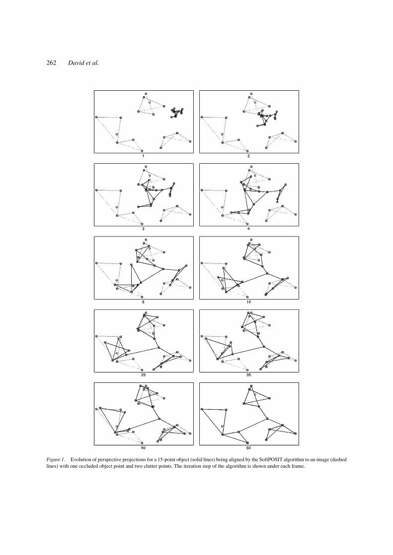
Figure 1 shows an example computation ofSoftPOSIT for an object with 15 points. Notice thatit would be impossible to make hard correspondencedecisions for the initial pose (frame 1), where the ob-ject’s image does not match the actual image at all.The deterministic annealing mechanism keeps all theoptions open until the two images are almost aligned.As another example of SoftPOSIT, Fig. 2 shows thetrajectory of the perspective projection of a cube beingaligned to an image of a cube.

In the following sections, we examine each step ofthe method. We then provide pseudocode for the al-gorithm. We then evaluate the algorithm using MonteCarlo simulations with various levels of clutter, oc-clusion and image noise, and finally we apply thealgorithm to some real imagery.

2. A New Formulation of the POSIT Algorithm

One of the building blocks of SoftPOSIT is the POSITalgorithm, presented in detail in DeMenthon and Davis(1995), which determines pose from known corre-spondences. The presentation given in DeMenthon andDavis (1995) requires that an object point with a knownimage be selected as the origin of the object coordinatesystem. This is possible with POSIT because corre-spondences are assumed to be known. Later, however,when we assume that correspondences are unknown,this will not be possible. Hence, we give a new for-mulation of the POSIT algorithm below that has nopreferential treatment of the object origin, and then we

262 David et al.

Figure 1. Evolution of perspective projections for a 15-point object (solid lines) being aligned by the SoftPOSIT algorithm to an image (dashedlines) with one occluded object point and two clutter points. The iteration step of the algorithm is shown under each frame.

SoftPOSIT: Simultaneous Pose and Correspondence Determination 263

Figure 2. The trajectory of the perspective projection of a cube(solid lines) being aligned by the SoftPOSIT algorithm to an imageof a cube (dashed lines), where one vertex of the cube is occluded.A simple object is used for the sake of clarity.

present a variant of this algorithm, still with knowncorrespondences, using the closed-form minimizationof an objective function. It is this objective functionwhich is modified in the next section to analyticallycharacterize the global pose-correspondence problem(i.e., without known correspondences) in a singleequation.

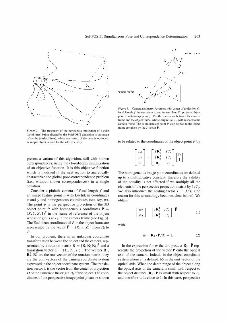
Consider a pinhole camera of focal length f andan image feature point p with Euclidean coordinatesx and y and homogeneous coordinates (wx, wy, w).The point p is the perspective projection of the 3Dobject point P with homogeneous coordinates P =(X, Y, Z , 1)T in the frame of reference of the objectwhose origin is at P0 in the camera frame (see Fig. 3).The Euclidean coordinates of P in the object frame arerepresented by the vector P̃ = (X, Y, Z )T from P0 toP .

In our problem, there is an unknown coordinatetransformation between the object and the camera, rep-resented by a rotation matrix R = [R1 R2 R3]T and atranslation vector T = (Tx , Ty, Tz)T. The vectors RT

1 ,RT

2 , RT3 are the row vectors of the rotation matrix; they

are the unit vectors of the camera coordinate systemexpressed in the object coordinate system. The transla-tion vector T is the vector from the center of projectionO of the camera to the origin P0 of the object. The coor-dinates of the perspective image point p can be shown

Figure 3. Camera geometry. A camera with center of projection O ,focal length f , image center c, and image plane �, projects objectpoint P onto image point p. T is the translation between the cameraframe and the object frame, whose origin is at P0 with respect to thecamera frame. The coordinates of point P with respect to the objectframe are given by the 3-vector P̃.

to be related to the coordinates of the object point P by

wx

wy

w

=

f RT1 f Tx

f RT2 f Ty

RT3 Tz

[

P̃1

].

The homogeneous image point coordinates are definedup to a multiplicative constant; therefore the validityof the equality is not affected if we multiply all theelements of the perspective projection matrix by 1/Tz .We also introduce the scaling factor s = f/Tz (thereason for this terminology becomes clear below). Weobtain

[wx

wy

]=

[sRT

1 sTx

sRT2 sTy

][P̃

1

](1)

with

w = R3 · P̃/Tz + 1. (2)

In the expression for w the dot product R3 · P̃ rep-resents the projection of the vector P̃ onto the opticalaxis of the camera. Indeed, in the object coordinatesystem where P is defined, R3 is the unit vector of theoptical axis. When the depth range of the object alongthe optical axis of the camera is small with respect tothe object distance, R3 · P̃ is small with respect to Tz ,and therefore w is close to 1. In this case, perspective

264 David et al.

projection gives results that are similar to the followingtransformation:[

x

y

]=

[sRT

1 sTx

sRT2 sTy

][P̃

1

]. (3)

This expression defines the scaled orthographic projec-tion p′ of the 3D point P . The factor s is the scaling fac-tor of this scaled orthographic projection. When s = 1,this equation expresses a transformation of points froman object coordinate system to a camera coordinate sys-tem, and uses two of the three object point coordinatesin determining the image coordinates; this is the defini-tion of a pure orthographic projection. With a factor sdifferent from 1, this image is scaled and approximatesa perspective image because the scaling is inverselyproportional to the distance Tz from the camera centerof projection to the object origin P0 (s = f/Tz).

The general perspective equation (Eq. (1)) can berewritten as

[ X Y Z 1 ]

[sR1 sR2

sTx sTy

]= [ wx wy ]. (4)

Assume that for each image point p with coordinatesx and y the corresponding homogeneous coordinate w

has been computed at a previous computation step andis known. Then we are able to calculate wx and wy,and the previous equation expresses the relationshipbetween the unknown pose components sR1, sR2, sTx ,sTy , and the known image components wx and wy andknown object coordinates X , Y , Z of P̃. If we know Mobject points Pk , k = 1, . . . , M , with Euclidean coor-dinates P̃k = (Xk, Yk, Zk)T, their corresponding imagepoints pk , and their homogeneous components wk , thenwe can then write two linear systems of M equationsthat can be solved for the unknown components of vec-tors sR1, sR2 and the unknowns sTx and sTy , providedthe rank of the matrix of object point coordinates is atleast 4. Thus, at least four of the points of the object forwhich we use the image points must be noncoplanar.After the unknowns sR1 and sR2 are obtained, we canextract s, R1, and R2 by imposing the condition that R1

and R2 must be unit vectors. Then we can obtain R3 asthe cross-product of R1 and R2:

s = (|sR1||sR2|)1/2 (geometric mean),

R1 = (sR1)/s, R2 = (sR2)/s,

R3 = R1 × R2,

Tx = (sTx )/s, Ty = (sTy)/s, Tz = f/s.

An additional intermediary step that improves perfor-mance and quality of results consists of using unit vec-tors R′

1 and R′2 that are mutually perpendicular and

closest to R1 and R2 in the least square sense. Thesevectors can be found by singular value decomposition(SVD) (see the Matlab code in DeMenthon and David(2001)).

How can we compute the wk components in Eq. (4)that determine the right-hand side rows (wk xk, wk yk)corresponding to image point pk? We saw that settingwk = 1 for every point is a good first step because itamounts to solving the problem with a scaled ortho-graphic model of projection. Once we have the poseresult for this first step, we can compute better esti-mates for the wk using Eq. (2). Then we can solve thesystem of Eq. (4) again to obtain a refined pose. Thisprocess is repeated, and the iteration is stopped whenthe process becomes stationary.

3. Geometry and Objective Function

We now look at a geometric interpretation of thismethod in order to propose a variant using an ob-jective function. As shown in Fig. 4, consider a pin-hole camera with center of projection at O , opticalaxis aligned with Oz, image plane � at distance ffrom O , and image center (principal point) at c. Con-sider an object, the origin of its coordinate systemat P0, a point P of this object, a corresponding im-age point p, and the line of sight L of p. The imagepoint p′ is the scaled orthographic projection of objectpoint P . The image point p′′ is the scaled orthographicprojection of point PL obtained by shifting P to theline of sight of p in a direction parallel to the imageplane.

One can show (see Appendix B) that the image planevector from c to p′ is

cp′ = s(R1 · P̃ + Tx , R2 · P̃ + Ty).

In other words, the left-hand side of Eq. (4) representsthe vector cp′ in the image plane. One can also showthat the image plane vector from c to p′′ is cp′′ =(wx, wy) = wcp. In other words, the right-hand sideof Eq. (4) represents the vector cp′′ in the image plane.The image point p′′ can be interpreted as a correctionof the image point p from a perspective projection toa scaled orthographic projection of a point PL locatedon the line of sight at the same distance as P . P is onthe line of sight L of p if, and only if, the image points

SoftPOSIT: Simultaneous Pose and Correspondence Determination 265

Figure 4. Geometric interpretation of the POSIT computation. Im-age point p′, the scaled orthographic projection of object point P ,is computed by the left-hand side of Eq. (4). Image point p′′, thescaled orthographic projection of point PL on the line of sight of p,is computed by the right-hand side of this equation. The equationis satisfied when the two points are superposed, which requires thatthe object point P be on the line of sight of image point p. Theplane of the figure is chosen to contain the optical axis and the lineof sight L . The points P0, P , P ′, and p′ are generally out of thisplane.

p′ and p′′ are superposed. Then cp′ = cp′′, i.e. Eq. (4)is satisfied.

When we try to match a set of object points Pk ,k = 1, . . . , M , to the lines of sight Lk of their imagepoints pk , it is unlikely that all or even any of the pointswill fall on their corresponding lines of sight, or equiva-lently that cp′

k = cp′′k or p′

kp′′k = 0. The least squares

solution of Eq. (4) for pose enforces these constraints.Alternatively, we can minimize a global objective func-tion E equal to the sum of the squared distancesd2

k =| p′kp′′

k | 2 between image points p′k and p′′

k :

E =∑

k

d2k =

∑k

|cp′k − cpk

′′|2

=∑

k

((Q1 · Pk − wk xk)2 + (Q2 · Pk − wk yk)2)

(5)

where we have introduced the vectors Q1, Q2, andPk with four homogeneous coordinates to simplify the

subsequent notation:

Q1 = s(R1, Tx ),

Q2 = s(R2, Ty),

Pk = (P̃k, 1).

We call Q1 and Q2 the pose vectors.Referring again to Fig. 4, notice that p′p′′ =

sP′P′′ = sPPL. Therefore minimizing this objectivefunction consists of minimizing the scaled sum ofsquared distances of object points to lines of sight,when distances are taken along directions parallel tothe image plane. This objective function is minimizediteratively. Initially, the wk are all set to 1. Then the fol-lowing two operations take place at each iteration step:

1. Compute the pose vectors Q1 and Q2 assuming theterms wk are known (Eq. (5)).

2. Compute the correction terms wk using the posevectors Q1 and Q2 just computed (Eq. (2)).

We now focus on the optimization of the pose vectorsQ1 and Q2. The pose vectors that will minimize theobjective function E at a given iteration step are thosefor which all the partial derivatives of the objectivefunction with respect to the coordinates of these vectorsare zero. This condition provides 4 × 4 linear systemsfor the coordinates of Q1 and Q2 whose solutions are

Q1 =( ∑

k

PkPTk

)−1( ∑k

wk xkPk

), (6)

Q2 =( ∑

k

PkPTk

)−1( ∑k

wk ykPk

). (7)

The matrix L = (∑

k PkPTk ) is a 4 × 4 matrix that can

be precomputed.With either method, the point p′′ can be viewed as

the image point p “corrected” for scaled orthographicprojection using w computed at the previous step ofthe iteration. The next iteration step finds the pose suchthat the scaled orthographic projection of each point Pis as close as possible to its corrected image point.

4. Pose Calculation with UnknownCorrespondences

When correspondences are unknown, each image fea-ture point p j can potentially match any of the object

266 David et al.

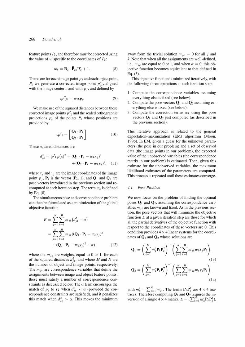
feature points Pk , and therefore must be corrected usingthe value of w specific to the coordinates of Pk :

wk = R3 · P̃k/Tz + 1. (8)

Therefore for each image point p j and each object pointPk we generate a corrected image point p′′

jk , alignedwith the image center c and with p j , and defined by

cp′′jk = wkcpj. (9)

We make use of the squared distances between thesecorrected image points p′′

jk and the scaled orthographicprojections p′

k of the points Pk whose positions areprovided by

cp′k =

[Q1 · Pk

Q2 · Pk

]. (10)

These squared distances are

d2jk = |p′

k p′jk|2 = (Q1 · Pk − wk x j )

2

+ (Q2 · Pk − wk y j )2, (11)

where x j and y j are the image coordinates of the imagepoint p j , Pk is the vector (P̃k, 1), and Q1 and Q2 arepose vectors introduced in the previous section and re-computed at each iteration step. The term wk is definedby Eq. (8).

The simultaneous pose and correspondence problemcan then be formulated as a minimization of the globalobjective function

E =N∑

j=1

M∑k=1

m jk(d2

jk − α)

=N∑

j=1

M∑k=1

m jk((Q1 · Pk − wk x j )2

+ (Q2 · Pk − wk y j )2 − α) (12)

where the m jk are weights, equal to 0 or 1, for eachof the squared distances d2

jk , and where M and N arethe number of object and image points, respectively.The m jk are correspondence variables that define theassignments between image and object feature points;these must satisfy a number of correspondence con-straints as discussed below. The α term encourages thematch of p j to Pk when d2

jk < α (provided the cor-respondence constraints are satisfied), and it penalizesthis match when d2

jk > α. This moves the minimum

away from the trivial solution m jk = 0 for all j andk. Note that when all the assignments are well-defined,i.e., m jk are equal to 0 or 1, and when α = 0, this ob-jective function becomes equivalent to that defined inEq. (5).

This objective function is minimized iteratively, withthe following three operations at each iteration step:

1. Compute the correspondence variables assumingeverything else is fixed (see below).

2. Compute the pose vectors Q1 and Q2 assuming ev-erything else is fixed (see below).

3. Compute the correction terms wk using the posevectors Q1 and Q2 just computed (as described inthe previous section).

This iterative approach is related to the generalexpectation-maximization (EM) algorithm (Moon,1996). In EM, given a guess for the unknown param-eters (the pose in our problem) and a set of observeddata (the image points in our problem), the expectedvalue of the unobserved variables (the correspondencematrix in our problem) is estimated. Then, given thisestimate for the unobserved variables, the maximumlikelihood estimates of the parameters are computed.This process is repeated until these estimates converge.

4.1. Pose Problem

We now focus on the problem of finding the optimalposes Q1 and Q2, assuming the correspondence vari-ables m jk are known and fixed. As in the previous sec-tion, the pose vectors that will minimize the objectivefunction E at a given iteration step are those for whichall the partial derivatives of the objective function withrespect to the coordinates of these vectors are 0. Thiscondition provides 4 × 4 linear systems for the coordi-nates of Q1 and Q2 whose solutions are

Q1 =(

M∑k=1

m ′kPkPT

k

)−1( N∑j=1

M∑k=1

m jkwk x j Pk

),

(13)

Q2 =(

M∑k=1

m ′kPkPT

k

)−1( N∑j=1

M∑k=1

m jkwk y j Pk

),

(14)

with m ′k = ∑N

j=1 m jk . The terms PkPTk are 4 × 4 ma-

trices. Therefore computing Q1 and Q2 requires the in-version of a single 4 × 4 matrix, L = (

∑Mk=1 m ′

kPkPTk ),

SoftPOSIT: Simultaneous Pose and Correspondence Determination 267

a fairly inexpensive operation (note that because theterm in column k and slack row N + 1 (see be-low) is generally greater than 0, m ′

k = ∑Nj=1 m jk is

generally not equal to 1, and L generally cannot beprecomputed).

4.2. Correspondence Problem

We next find the optimal values of the correspondencevariables m jk assuming that the parameters d2

jk in theexpression for the objective function E are known andfixed. Our aim is to find a zero-one assignment (ormatch) matrix, m = {m jk}, that explicitly specifies thematchings between a set of N image points and a set ofM object points, and that minimizes the objective func-tion E . m has one row for each of the N image points p j

and one column for each of the M object points Pk . Theassignment matrix must satisfy the constraint that eachimage point match at most one object point, and viceversa. By adding an extra row and column to m, slackrow N + 1 and slack column M + 1, these constraintscan be expresses as m jk ∈ {0, 1} for 1 ≤ j ≤ N + 1and 1 ≤ k ≤ M + 1,

∑M+1i=1 m ji = 1 for 1 ≤ j ≤ N ,

and∑N+1

i=1 mik = 1 for 1 ≤ k ≤ M . A value of 1 in theslack column M +1 at row j indicates that image pointp j has not found any match among the object points.A value of 1 in the slack row N + 1 at column k indi-cates that the object point Pk is not seen in the imageand does not match any image feature. The objectivefunction E will be minimum if the assignment matrixmatches image and object points with the smallest dis-tances d2

jk . This problem can be solved by the iterativesoftassign technique (Gold and Rangarajan, 1996; Goldet al., 1998). The iteration for the assignment matrix mbegins with a matrix m0 = {m0

jk} in which elementm0

jk is initialized to exp(−β(d2jk − α)), with β very

small, and with all elements in the slack row and slackcolumn set to a small constant. See Gold et al. (1998)for an analytical justification. The exponentiation hasthe effect of ensuring that all elements of the assign-ment matrix are positive. The parameter α determineshow far apart two points must be before they are con-sidered unmatchable. It should be set to the maximumallowed squared distance between an image point andthe matching projected object point. This should be afunction of the noise level in the image. With normallydistributed x and y noise of zero mean and standard de-viation σ , the squared distance between a true 2D pointand the measured 2D point has a χ2 distribution with2 degrees of freedom (Hartley and Zisserman, 2000,

p. 549). Thus, to ensure with probability 0.99 that ameasured point is allowed to match to a true point, weshould take α = 9.21 × σ 2. Since initial pose esti-mates can be very inaccurate, the initial distances d2

jkfor correct correspondences will likely be greater thanα. However, no correspondences will be initially ruledout as β is initially very small; a small β makes all m0

jknearly equal with slightly larger values being assignedto correspondences having small d2

jk . As β increases,and presumably the accuracy of the pose as well, theinfluence of α becomes more significant until the endof the iteration where correspondences with d2

jk > α

are rejected.The continuous matrix m0 converges toward the dis-

crete assignment matrix m due to two mechanisms thatare used concurrently:

1. First, a technique due to Sinkhorn (1964) is applied.When each row and column of a square correspon-dence matrix is normalized (several times, alternat-ingly) by the sum of the elements of that row orcolumn respectively, the resulting matrix has posi-tive elements with all rows and columns summingto 1.

2. The term β is increased as the iteration proceeds. Asβ increases and each row or column of m0 is renor-malized, the terms m0

jk corresponding to the small-est d2

jk tend to converge to 1, while the other termstend to converge to 0. This is a deterministic an-nealing process (Geiger and Yuille, 1991) known assoftmax (Bridle, 1990). This is a desirable behavior,since it leads to an assignment of correspondencesthat satisfy the matching constraints and whose sumof distances is minimized.

This combination of deterministic annealing andSinkhorn’s technique in an iteration loop was calledsoftassign by Gold and Rangarajan (1996) and Goldet al. (1998). The matrix m resulting from an itera-tion loop that comprises these two substeps is the as-signment that minimizes the global objective functionE = ∑J

j=1

∑Kk=1 m jk(d2

jk − α). As the pseudocode inAlgorithm 1 shows, these two substeps are interleavedin the iteration loop of SoftPOSIT, along with the sub-steps that find the optimal pose and correct the imagepoints by scaled orthographic distortions.

At the end of the SoftPOSIT iteration, the matrixm will be very close to a true zero-one assignmentmatrix. If desired, one can obtain discrete correspon-dences from this matrix and then apply any algorithm

268 David et al.

Algorithm 1 SoftPOSIT pseudocode.

1. Inputs:

(a) List of M object points, Pk = (Xk, Yk, Zk, 1)T = (P̃k, 1), 1 ≤ k ≤ M ,(b) List of N image points, p j = (x j , y j ), 1 ≤ j ≤ N .

2. Initialize:

(a) Slack elements of assignment matrix m0 to γ = 1/(max{M, N } + 1),(b) β to β0 (β0 ≈ 0.0004 if nothing is known about the pose, and is larger if an initial pose can be guessed),(c) Pose vectors Q1 and Q2 using the expected pose or a random pose within the expected range,(d) wk = 1, 1 ≤ k ≤ M .

3. Do A until β > βfinal (βfinal ≈ 0.5) (Deterministic annealing loop)

(a) Compute squared distances d2jk = (Q1 · Pk − wk x j )2 + (Q2 · Pk − wk y j )2, 1 ≤ j ≤ N , 1 ≤ k ≤ M .

(b) Compute m0jk = γ exp (−β (d2

jk − α)), 1 ≤ j ≤ N , 1 ≤ k ≤ M .(c) Do B until ‖mi − mi−1‖ small (Sinkhorn’s method)

i. Normalize nonslack rows of m: mi+1jk = mi

jk/∑M+1

k=1 mijk , 1 ≤ j ≤ N , 1 ≤ k ≤ M + 1.

ii. Normalize nonslack columns of m: mi+1jk = mi+1

jk /∑N+1

j=1 mi+1jk , 1 ≤ j ≤ N + 1, 1 ≤ k ≤ M .

(d) End Do B

4. Compute the 4 × 4 matrix L = (∑M

k=1 m ′kPkPT

k ) with m ′k = ∑N

j=1 m jk .5. Compute L−1.6. Compute Q1 = (Q1

1, Q21, Q3

1, Q41)T = L−1(

∑Nj=1

∑Mk=1 m jkwk x j Pk).

7. Compute Q2 = (Q12, Q2

2, Q32, Q4

2)T = L−1(∑N

j=1

∑Mk=1 m jkwk y j Pk).

8. Compute s = (‖(Q11, Q2

1, Q31)‖‖(Q1

2, Q22, Q3

2)‖)1/2.9. Compute R1 = (Q1

1, Q21, Q3

1)T/s, R2 = (Q12, Q2

2, Q32)T/s, R3 = R1 × R2.

10. Compute Tx = Q41/s, Ty = Q4

2/s, Tz = f/s.11. Compute wk = R3 · P̃k/Tz + 1, 1 ≤ k ≤ M .12. β = βupdateβ (βupdate ≈ 1.05) .13. End Do A14. Outputs:

(a) Rotation matrix R = [R1 R2 R3]T,(b) Translation vector T = (Tx , Ty, Tz),(c) Assignment matrix m = {m jk} between the list of image points and the list of object points.

that computes pose from known correspondences toobtain the most accurate pose possible.

The SoftPOSIT algorithm has a number of ad-vantages over conventional nonlinear optimization al-gorithms. Typical nonlinear constrained optimizationproblems are defined by the minimization of an ob-jective function on a feasible region that is definedby equality and inequality constraints. The simulta-neous pose and correspondence problem requires the

minimization of an objective function subject to theconstraint that the final assignment matrix must be azero-one matrix whose rows and columns each sumto one. A constraint such as this would be impossibleto express using equality and inequality constraints.SoftPOSIT uses deterministic annealing to convert thisdiscrete problem into a continuous one that is indexedby the control parameter β. This has two advantages.First, it allows solutions to the simpler continuous

SoftPOSIT: Simultaneous Pose and Correspondence Determination 269

problem to slowly transform into a solution to thediscrete problem. Secondly, many local minima areavoided by minimizing an objective function that ishighly smoothed during the early phases of the opti-mization but which gradually transforms into the orig-inal objective function and constraints at the end of theoptimization.

5. Random Start SoftPOSIT

The SoftPOSIT algorithm performs a search startingfrom an initial guess for the object’s pose. The globalobjective function that this search attempts to mini-mize (Eq. (12)) has many local optima. The determin-istic annealing process initially smooths this objectivefunction, which eliminates shallow local optima andgreatly improves SoftPOSIT’s chances of finding theglobal optimum if it is near the initial guess. How-ever, one cannot expect to smooth the objective func-tion to the extent that it has a single local optimum at thesame location as the global optimum of the unsmoothedobjective function: too much smoothing can hide theglobal optimum and lead the search away from thisoptimum just as quickly as no smoothing at all. Thus,the search performed by SoftPOSIT is local, and thereis no guarantee of finding the global optimum given asingle initial guess.

Given an initial pose that lies in a valley of thesmoothed objective function, we expect the algorithmto converge to the minimum associated with that val-ley. To examine other valleys, we must start with pointsthat lie in them. The size and shape of these valleysdepends on a number of factors including the param-eters of the annealing schedule (β0 and βupdate), thecomplexity of the 3D object, the amount of object oc-clusion, the amount of image clutter, and the imagemeasurement noise. A common method of searchingfor a global optimum, and the one used here, is torun the local search algorithm starting from a numberof different initial guesses, and keep the first solutionthat meets a specified termination criterion. Our initialguesses span the range [−π, π ] for the three Euler ro-tation angles, and a 3D space of translations known tocontain the true translation. We use a pseudo-randomnumber generator to generate random 6-vectors in aunit 6D hypercube. (Using a quasi-random (Morokoffand Caflisch, 1994) coverage of the hypercube didnot improve the performance of the algorithm.) Thesepoints are then scaled to cover the expected rangesof translation and rotation. The rest of this section

describes the search termination criterion that weuse.

5.1. Search Termination

Ideally, one would like to repeat the search from a newstarting point whenever the number of object-to-imagecorrespondences determined by the search is not max-imal. With real data, however, one usually does notknow what this maximal number is. Instead, we repeatthe search when the number of object points that matchimage points is less than some threshold tm . Due toocclusion and imperfect image feature extraction algo-rithms, not all object points will be detected as featuresin an image of that object. Let the fraction of detectedobject features be

pd = number of object points detected as image features

total number of object points.

In the Monte Carlo simulations described below, pd isknown. With real imagery, however, pd must be esti-mated based on the scene complexity and on the reli-ability of the image processing algorithm in detectingobject features.

We terminate the search for better solutions when thecurrent solution is such that the number of object pointsthat match any image point is greater than or equal tothe threshold tm = ρpd M , where ρ determines whatpercent of the detected object points must be matched(0 < ρ ≤ 1), and M is the total number of object points,so that pd M is the number of detected object points. ρ

accounts for measurement noise that typically preventssome detected object features from being matched evenwhen a good pose is found. In the experiments dis-cussed below, we take ρ = 0.8. This test is not perfect,as it is possible for a pose to be very accurate even whenthe number of matched points is less than this threshold;this occurs mainly in cases of high noise. Conversely,a wrong pose may be accepted when the ratio of clutterfeatures to detected object points is high. It has beenobserved, however, that these situations are relativelyuncommon.

We note that Grimson and Huttenlocher (1991) havederived an expression for a threshold on the numberof matched object points necessary to accept a localoptimum; their expression is a function of the numbersof image and object points and of the sensor noise, andguarantees with a specified probability that the globallyoptimal solution has been found.

270 David et al.

5.2. Early Search Termination

The deterministic annealing loop of the SoftPOSIT al-gorithm iterates over a range of values for the annealingparameter β. In the experiments reported here, β is ini-tialized to β0 = 0.0004 and is updated according toβ = 1.05 × β, and the annealing iteration ends whenthe value of β exceeds 0.5. (The iteration may end ear-lier if convergence is detected.) This means that theannealing loop can run for up to 147 iterations. It isusually the case that, by viewing the original imageand, overlaid on top of it, the projected object pointsproduced by SoftPOSIT, a person can determine veryearly (e.g., around iteration 30) whether or not the al-gorithm is going to converge to the correct pose. Itis desired that the algorithm make this determinationitself, so that whenever it detects that it seems to beheading down an unfruitful path, it can end the cur-rent search for a local optimum and restart from a newrandom initial condition, thereby saving a significantamount of processing time.

A simple test is performed at each iteration ofSoftPOSIT to determine if it should continue with theiteration or restart. At the i th step of the SoftPOSITiteration, the match matrix mi = {mi

j,k} is used topredict the final correspondences of object to imagepoints. Upon convergence of SoftPOSIT, one wouldexpect image point j to correspond to object point kif mi

j,k > miu,v for all u �= j and all v �= k (though

this is not guaranteed). The number of predicted cor-respondences at iteration i , ni , is just the number ofpairs ( j, k) that satisfy this relation. We then define thematch ratio at step i as ri = ni/(pd K ) where pd is thefraction of detected object features as defined above.

The early termination test centers around thismatch ratio measure. This measure is commonly used(Grimson and Huttenlocher, 1991) at the end of a localsearch to determine if the current solution for corre-spondence and pose is good enough to end the searchfor the global optimum. We, however, use this metricwithin the local search itself. Let C denote the eventthat the SoftPOSIT algorithm eventually converges tothe correct pose. Then the algorithm restarts after thei th step of the iteration if P(C | ri ) < λP(C), where0 < λ ≤ 1. That is, the search is restarted from anew random starting condition whenever the posteriorprobability of eventually finding a correct pose given ri

drops to less than some fraction of the prior probabilityof finding the correct pose. Notice that a separate pos-terior probability function is required for each iteration

step because the ability to predict the eventual outcomeusing ri changes as the iterations progress. Althoughthis test may result in the termination of some localsearches which would have eventually produced goodposes, it is expected that the total time required to finda good pose will be less. Our experiments show thatthis is indeed the case; we obtain a speedup by a factorof 2.

Early termination is achieved by stopping the itera-tion when ri falls below a threshold that is a functionof the iteration step i . For each i , this threshold is thevalue of ri for which P(C | ri ) = λP(C). The posteriorprobability function for the i th step of the iteration canbe computed from P(C), the prior probability of find-ing a correct pose on one random local search, and fromP(ri | C) and P(ri | C̄), the probabilities of observinga particular match ratio on the i th iteration step giventhat the eventual pose is either correct or incorrect, re-spectively:

P(C | ri ) = P(C)P(ri | C)

P(C)P(ri | C) + P(C̄)P(ri | C̄).

P(C), P(C̄), P(ri | C), and P(ri | C̄) are estimated inMonte Carlo simulations of the algorithm in which thenumber of object points and the levels of image clut-ter, occlusion, and noise are all varied. The details ofthese simulations are described in Section 6. To esti-mate P(ri | C) and P(ri | C̄), the algorithm is repeat-edly run on random test data. For each test, the valuesof the match ratio ri computed at each iteration arerecorded. Once a SoftPOSIT iteration is completed,ground truth information is used to determine whetheror not the correct pose was found. If the pose is correct,the recorded values of ri are used to update histogramsrepresenting the probability functions P(ri | C); oth-erwise, histograms representing P(ri | C̄) are updated.Upon completing this training, the histograms are nor-malized. P(C) is easily estimated based on the percentof the random tests that produced the correct pose. Wealso have P(C̄) = 1 − P(C). Two of these estimatedprobability functions are shown in Fig. 5.

6. Experiments

The two most important questions related to the perfor-mance of the SoftPOSIT algorithm are (a) How oftendoes it find a “good” pose? and (b) How long doesit take? Both of these issues are investigated in thissection.

SoftPOSIT: Simultaneous Pose and Correspondence Determination 271

Figure 5. Probability functions estimated for (a) the first iteration, and (b) the 31st iteration, of the SoftPOSIT algorithm.

6.1. Monte Carlo Evaluation

The random-start SoftPOSIT algorithm has been ex-tensively evaluated in Monte Carlo simulations. Thesimulations and the performance of the algorithm arediscussed in this section. The simulations are charac-terized by the five parameters: nt , M , pd , pc, and σ .nt is the number of independent random trials to per-form for each combination of values of the remain-ing four parameters. M is the number of points (ver-tices) in a 3D object. pd is the probability that theimage of any particular object point will be detectedas a feature point in the image. pd takes into accountocclusion of the 3D object points as well as the factthat real image processing algorithms do not detect alldesired feature points, even when the corresponding3D points are not occluded. pc is the probability thatany particular image feature point is clutter, that is,is not the image of some 3D object point. Finally, σ

is the standard deviation of the normally distributednoise in the x and y coordinates of the non-clutterfeature points, measured in pixels for a 1000 × 1000image, generated by a simulated camera having a37-degree field of view (a focal length of 1500 pix-els). The current tests were performed with nt = 100,M ∈ {20, 30, 40, 50, 60, 70, 80}, pd ∈ {0.4, 0.6, 0.8},pc ∈ {0.2, 0.4, 0.6}, and σ ∈ {0.5, 1.0, 2.5}. (Be-cause corner detection algorithms typically claim ac-curacies of 1/10th of a pixel (Brand and Mohr,1994), these values of σ are conservative.) With

these parameters, 18,900 independent trials were per-formed.

For each trial, a 3D object is created in which theM object vertices are randomly located in a spherecentered at the object’s origin. Because this algorithmworks with points, not with line segments, it is only theobject vertices that are important in the current tests.However, to make the images produced by the algo-rithm easier to understand, we draw each object vertexas connected by an edge to the two closest of the re-maining object vertices. These connecting edges arenot used by the SoftPOSIT algorithm. The object isthen rotated into some arbitrary orientation, and trans-lated to some random point in the field of view of thecamera. Next, the object is projected into the imageplane of the camera; each projected object point is de-tected with probability pd . For those points that aredetected, normally distributed noise with mean zeroand standard deviation σ is added to both the x andy coordinates of the feature points. Finally, randomlylocated clutter feature points are added to the true (non-clutter) feature points, so that 100 × pc percent of thetotal number of feature points are clutter; to achievethis, Mpd pc/(1− pc) clutter points must be added. Theclutter points are required to lie in the general vicinityof the true feature points. However, to prevent the clut-ter points from replacing missing true feature points,each clutter point must be further than

√2σ from any

projected object point, whether or not the point wasdetected. Figure 6 shows a few examples of cluttered

272 David et al.

Figure 6. Typical images of randomly generated objects and images. The black points are projected object points and the white points (circles)are clutter points. The black lines, which connect the object points, are included in these pictures to assist the reader in understanding the pictures;they are not used by the algorithm. The number of points in the objects are 20 for (a), 30 for (b), 40 for (c), 50 for (d) and (e), 60 for (f) and(g), 70 for (h), and 80 for (i). In all cases shown here, pd = 1.0 and pc = 0.6. This is the best case for occlusion (none), but the worst case forclutter. In the actual experiments, pd and pc vary.

images of random objects that are typical of those usedin our experiments.

In our experiments, we consider a pose to be goodwhen it allows tm (defined in Section 5.1) or more of theM object points to be matched to some image point. Thenumber of random starts (random initial pose guesses)for each trial was limited to 10,000. Thus, if a goodpose is not found after 10,000 starts, the algorithm givesup. (As discussed below, far fewer starts are typicallyrequired for success.) Figures 7 and 8 show a number ofexamples of poses found by SoftPOSIT when random6-vectors are used as the initial guesses for pose.

Figure 9 shows the success rate of the algorithm (per-cent of trials for which a good pose was found in 10,000starts, given no knowledge of the correct pose) as afunction of the number of object points for σ = 2.5and for all combinations of the parameters pd and pc.(The algorithm performs a little better for σ = 0.5 andσ = 1.0.) It can be seen from this figure that, for morethan 92% of the different combinations of simulationparameters, a good pose is found in 90% or more of theassociated trials. For the remaining 8% of the tests, agood pose is found in 75% or more of the trials. Over-all, a good pose was found in 96.4% of the trials. As

SoftPOSIT: Simultaneous Pose and Correspondence Determination 273

Figure 7. Projected objects and cluttered images for which SoftPOSIT was successful. The small circles are the image points (includingprojected object and clutter) to which the objects must be matched. The light gray points and lines show the projections of the objects in theinitial poses (random guesses) which lead to good poses being found. The black points and lines show the projections of the objects in the goodposes that are found. The black points that are not near any circle are occluded object points. Circles not near any black point are clutter. Again,the gray and black lines are included in these pictures to assist the reader in understanding the pictures; they are not used by the algorithm. TheMonte Carlo parameters for these tests are pd = 0.6, pc = 0.4, σ = 2.5, M = 30 for (a) and (b), M = 50 for (c) and (d).

expected, the higher the occlusion rate (lower pd ) andthe clutter rate (higher pc), the lower the success rate.For the high-clutter tests, the success rate increases asthe number of object points decreases. This is due tothe algorithm’s ability to more easily match a smallnumber of object points to clutter than a large numberof object points to the same level of clutter.

Figure 10 shows the average number of random startsrequired to find a good pose. These numbers generallyincrease with increasing image clutter and occlusion.

However, for the reason given in the previous para-graph, the performance for small numbers of objectpoints is better at higher levels of occlusion and clut-ter. Other than in the highest occlusion and clutter case,the mean number of starts is about constant or increasesvery slowly with increasing number of object points.Also, there does not appear to be any significant in-crease in the standard deviation of the number of ran-dom starts as the number of object points increases.The mean number of starts over all of the tests is

274 David et al.

Figure 8. More complex objects and cluttered images for which SoftPOSIT was successful. The Monte Carlo parameters for these tests arepd = 0.6, pc = 0.4, σ = 2.5 and M = 70 for (a) and (b), M = 80 for (c) and (d).

approximately 500; the mean exceeds 1100 starts onlyin the single hardest case. Figure 11 shows the samedata but plotted as a function of the number of imagepoints. Again, except for the two highest occlusion andclutter cases, the mean number of starts is about con-stant or increases very slowly as the number of imagepoints increases.

6.2. Run Time Comparison

The RANSAC algorithm (Fischler and Bolles, 1981)is the best known algorithm to compute object posegiven 3D object and 2D image points when correspon-dences are not known in advance. In this section, we

compare the expected run time1 of SoftPOSIT to that ofRANSAC for each of the simulated data sets discussedin Section 6.1.

The mean run time of SoftPOSIT on each of thesedata sets was recorded during the Monte Carlo exper-iments. As will be seen below, to have run RANSACon each of these data sets would have required a pro-hibitive amount of time. This was not necessary, how-ever, since we can accurately estimate the number ofrandom samples of the data that RANSAC will exam-ine when solving any particular problem. The expectedrun time of RANSAC is then the product of that numberof samples with the expected run time on one sampleof that data.

SoftPOSIT: Simultaneous Pose and Correspondence Determination 275

Figure 9. Success rate as a function of the number of object pointsfor fixed values of pd and pc . (Note that pd and pc are denoted by Dand C , respectively, in the legend of this figure and in the next fewfigures.)

The computational complexity of a pose problem de-pends on the three parameters M , pd , and pc definedin Section 6.1. (Recall that pd and pc determine N ,the number of image points.) For each combination ofthese three parameters, we need to determine the ex-pected run time of RANSAC for a single sample ofthree object points and three image points2 from thatdata. This was accomplished by running RANSAC onmany random samples generated using the same set of

Figure 10. Number of random starts required to find a good pose as a function of the number of object points for fixed values of pd and pc .(a) Mean. (b) Standard deviation.

three complexity parameters. The time per sample fora given problem complexity is estimated as the totaltime used by RANSAC to process those samples (ex-cluding time for initialization) divided by the numberof samples processed.

We now estimate how many samples RANSAC willexamine for problems of a particular complexity. InAppendix A, we compute the probability, p, as a func-tion of M , pd , and pc, that a random sample of threeobject points and three image points consists of threecorrect correspondences. Then, the number of randomsamples of correspondence triples that must be exam-ined by RANSAC in order to ensure with probability zthat at least one correct correspondence triple will beexamined is

s1(z, p) = log(1 − z)

log(1 − p).

Some implementations of RANSAC will halt as soonas the first good sample is observed, thus reducing therun time of the algorithm. In this case, the expectednumber of random samples that will be examined inorder to observe the first good sample is

s2(p) = 1

p.

Note that for all values of M , pd , and pc thatwe consider here, and for z ≥ 0.75 (the smallest

276 David et al.

Figure 11. Number of random starts required to find a good pose as a function of the number of image points for fixed values of pd and pc .(a) Mean. (b) Standard deviation.

observed success rate for SoftPOSIT), s2(p) < s1(z, p).A RANSAC algorithm using s2 will always be fasterthan one using s1, but it will not be as robust sincerobustness increases with the number of samples ex-amined. In the following, the run times of SoftPOSITand RANSAC are compared using both s1 and s2

to determine the number of samples that RANSACexamines.

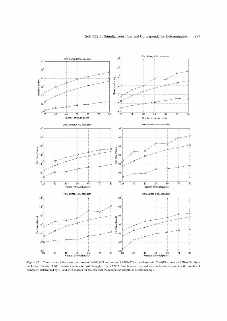
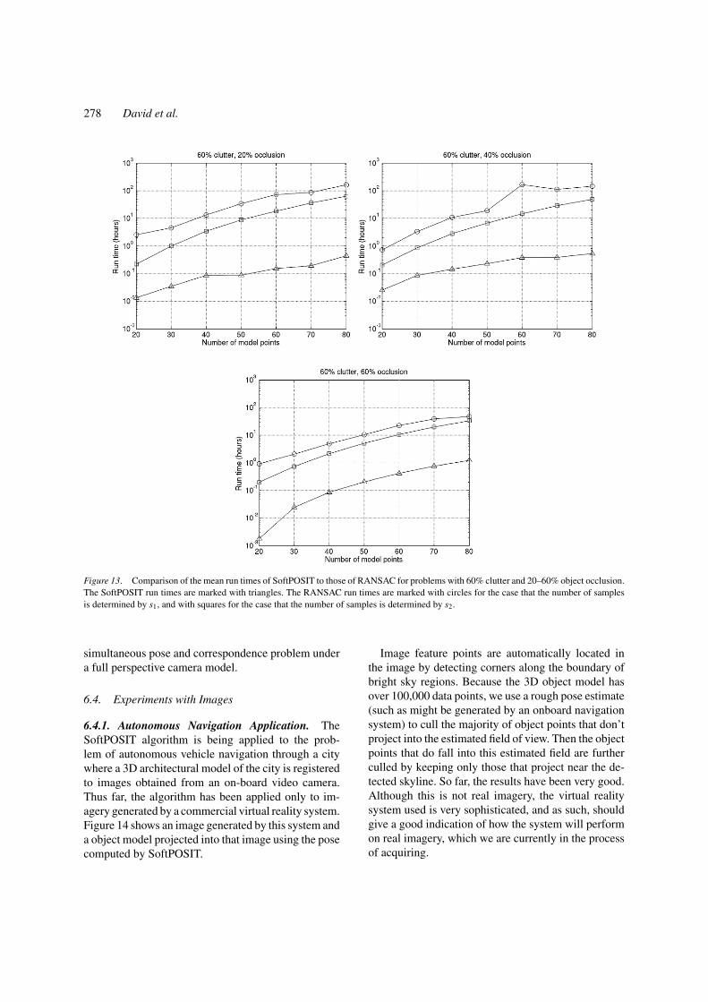
For a data set with complexity given by M , pd , andpc, SoftPOSIT has a given observed success rate whichwe denote by zsoftPOSIT(M, pd , pc) (see Fig. 9). Sincewe did not run RANSAC on this data, we can’t com-pare the success rates of SoftPOSIT and RANSACfor a given fixed amount of run time. However, wecan compare the mean run time required by bothto achieve the same rate of success on problems ofthe same complexity by estimating the run time ofRANSAC when its required probability of success isz = zsoftPOSIT(M, pd , pc). These run times are shown inFigs. 12 and 13. From these figures, it can be seen thatthe RANSAC algorithm requires one to three orders ofmagnitude more run time than SoftPOSIT for problemswith the same level of complexity in order to achievethe same level of success. Furthermore, for the majorityof the complexity cases, run time as a function of inputsize increases at a faster rate for the RANSAC algo-rithms than for the SoftPOSIT algorithm. The totalityof Monte Carlo experiments described in Section 6.1required about 30 days for SoftPOSIT to complete.

From this analysis it can be estimated that a RANSACalgorithm which examines s1 samples would requireabout 19.4 years to complete the same experiments,and a RANSAC algorithm which examines s2 sampleswould require about 4.5 years. Clearly, it would nothave been practical to run RANSAC on all of theseexperiments.

6.3. Algorithm Complexity

The run-time complexity of a single invocation of Soft-POSIT is O(M N ) where M is the number of objectpoints and N is the number of image points; this is be-cause the number of iterations on all of the loops in thepseudocode in Algorithm 1 are bounded by a constant,and each line inside a loop is computed in time at mostO(M N ). As shown in Figs. 10 and 11, the mean numberof random starts (invocations of SoftPOSIT) requiredto find a good pose in the worst (hardest) case, to en-sure a probability of success of at least 0.95, appears tobe bounded by a function that increases linearly withthe size of the input; in the other cases, the mean num-ber of random starts is approximately constant. Thatis, the mean number of random starts is O(N ), as-suming that M < N , as is normally the case. Thenthe run-time complexity of SoftPOSIT with randomstarts is O(M N 2). This is a factor of N better than thecomplexity of any published algorithm that solves the

SoftPOSIT: Simultaneous Pose and Correspondence Determination 277

Figure 12. Comparison of the mean run times of SoftPOSIT to those of RANSAC for problems with 20–40% clutter and 20–60% objectocclusion. The SoftPOSIT run times are marked with triangles. The RANSAC run times are marked with circles for the case that the number ofsamples is determined by s1, and with squares for the case that the number of samples is determined by s2.

278 David et al.

Figure 13. Comparison of the mean run times of SoftPOSIT to those of RANSAC for problems with 60% clutter and 20–60% object occlusion.The SoftPOSIT run times are marked with triangles. The RANSAC run times are marked with circles for the case that the number of samplesis determined by s1, and with squares for the case that the number of samples is determined by s2.

simultaneous pose and correspondence problem undera full perspective camera model.

6.4. Experiments with Images

6.4.1. Autonomous Navigation Application. TheSoftPOSIT algorithm is being applied to the prob-lem of autonomous vehicle navigation through a citywhere a 3D architectural model of the city is registeredto images obtained from an on-board video camera.Thus far, the algorithm has been applied only to im-agery generated by a commercial virtual reality system.Figure 14 shows an image generated by this system anda object model projected into that image using the posecomputed by SoftPOSIT.

Image feature points are automatically located inthe image by detecting corners along the boundary ofbright sky regions. Because the 3D object model hasover 100,000 data points, we use a rough pose estimate(such as might be generated by an onboard navigationsystem) to cull the majority of object points that don’tproject into the estimated field of view. Then the objectpoints that do fall into this estimated field are furtherculled by keeping only those that project near the de-tected skyline. So far, the results have been very good.Although this is not real imagery, the virtual realitysystem used is very sophisticated, and as such, shouldgive a good indication of how the system will performon real imagery, which we are currently in the processof acquiring.

SoftPOSIT: Simultaneous Pose and Correspondence Determination 279

Figure 14. Registration of a 3D city model to an image generated by a virtual reality system. Using the initial guess for the model’s pose,the 3D model vertices that project near the detected skyline in the image are selected to be matched to image points along this skyline. (a)Original image from the virtual reality system. (b) Selected model lines and points (white) projected into this image using the pose computedby SoftPOSIT.

6.4.2. Robot Docking Application. The robot dock-ing application requires that a small robot drive ontoa docking platform that is mounted on a larger robot.Figure 15 shows a small robot docking onto a largerrobot. In order to accomplish this, the small robot mustdetermine the relative pose of the large robot. This is

done by using SoftPOSIT to align a 3D model of thelarge robot to corner points extracted from an image ofthe large robot.

The model of the large robot consists of a set of 3Dpoints that are extracted from a triangular faceted modelof the robot which was generated by a commercial

280 David et al.

Figure 15. A small robot docking onto a larger robot.

Figure 16. An image of the large robot as seen from the small robot’s point of view. Long straight lines detected in the image are shown inwhite, and their intersections, which ideally should correspond to vertices in the 3D object, are shown as white circles with black centers.

SoftPOSIT: Simultaneous Pose and Correspondence Determination 281

Figure 17. The initial guess at the robot’s pose (a) that leads to the correct pose as shown in (b).

CAD system. To detect the corresponding points inthe image, lines are first detected using a combinationof the Canny edge detector, the Hough transform, anda sorting procedure used to rank the lines produced bythe Hough transform. Corners are then found at theintersections of those lines that satisfy simple length,proximity, and angle constraints. Figure 16 shows the

lines and corner points detected in one image of thelarge robot. In this test there are 70 points in the ob-ject; 89% of these are occluded (or not detected inthe image), and 58% of the image points are clutter.Figure 17(a) shows the initial guess generated by Soft-POSIT which led to the correct pose being found, andFig. 17(b) shows this correct pose.

282 David et al.

7. Conclusions

We have developed and evaluated the SoftPOSIT al-gorithm for determining the poses of objects from im-ages. The correspondence and pose calculation com-bines into one efficient iterative process the softassignalgorithm for determining correspondences and thePOSIT algorithm for determining pose. This algorithmwill be used as a component in an object recognitionsystem.

Our evaluation indicates that the algorithm performswell under a variety of levels of occlusion, clutter,and noise. The algorithm has been tested on syntheticdata for an autonomous navigation application, andwe are currently collecting real imagery for furthertests with this application. The algorithm has also beentested in an autonomous docking application with goodresults.

The complexity of SoftPOSIT has been empiricallydetermined to be O(M N 2). This is better than anyknown algorithm that solves the simultaneous pose andcorrespondence problem for a full perspective cameramodel. More data should be collected to further vali-date this claim.

Future work will involve extending the SoftPOSITalgorithm to work with lines in addition to points. Weare also interested in performing a more thorough com-parison of the performance of SoftPOSIT to that ofcompeting algorithms.

Appendix A: The Complexity of theHypothesize-And-Test Approach

The asymptotic run time complexity of the generalhypothesize-and-test approach to model-to-image reg-istration is derived in this appendix. We first define afew parameters:

M is the number of 3D object points,N is the number of image points,pd is the fraction of object points that are present (non-

occluded) in the image,R is the desired probability of success (i.e., of finding

a good pose).

Given a set of data with outlier rate w, it is wellknown (Fischler and Bolles, 1981) that the number kof random samples of the data of size n that must beexamined in order to ensure with probability z that at

least one of those samples is outlier-free is

k = log(1 − z)

log(1 − (1 − w)n).

We need to determine how this number of samples de-pends on M , N , pd , and R for the hypothesize-and-testalgorithm for large values of M and N .

Because we assume that the hypothesize-and-test al-gorithm has no a priori information about which cor-respondences are correct, correspondences are formedfrom randomly chosen object and image points. We as-sume that three correspondences are used to estimatethe object’s pose. Let S = pd M be the number of de-tected (non-occluded) object points in the image. For acorrespondence to be correct, two conditions must besatisfied: the object point must be non-occluded and theimage point must correspond to the object point. Theprobability that the nth (n = 1, 2, 3) randomly chosencorrespondence is correct given that all previously cho-sen correspondences are also correct is the probabilitythat these two conditions are satisfied, which is

S − n + 1

M − n + 1· 1

N − n + 1.

Then the probability that any sample consists of threecorrect correspondences is

S(S − 1)(S − 2)

M(M − 1)(M − 2)N (N − 1)(N − 2)≈ S3

M3 N 3

=(

pd

N

)3

.

The probability that each of T random samples is bad(i.e., each includes at least one incorrect correspon-dence) is (

1 −(

pd

N

)3)T

.

Thus to ensure with probability R that at least one ofthe randomly chosen samples consists of three correctcorrespondences, we must examine T samples where

1 −(

1 −(

pd

N

)3)T

≥ R.

Solving for T, we get

T ≥ log(1 − R)

log(1 − ( pd

N

)3) .

SoftPOSIT: Simultaneous Pose and Correspondence Determination 283

Noting that (pd/N )3 is always less that 10−4 in ourexperiments, and using the approximation log(1−x) ≈−x for x small, the number of samples that need to beexamined is

T ≈(

N

pd

)3

log

(1

1 − R

).

Since each sample requires O(M log N ) time for back-projection and verification (assuming an O(log N )nearest neighbor algorithm (Arya et al., 1998) is used tosearch for image points close to each projected objectpoint), the complexity of the general hypothesize-and-test algorithm is

(N

pd

)3

log

(1

1 − R

)× O(M log N ) =O(M N 3 log N ).

Appendix B: Scaled Orthographic Image Points

Here we give a geometric interpretation of the rela-tion between perspective and scaled orthographic im-age points. Consider Fig. 4. A plane �′ parallel to theimage plane � is chosen to pass through the origin P0

of the object coordinate system. This plane cuts thecamera axis at H (OH = Tz). The point P projectsinto P ′ on plane �′, and the image of P ′ on the imageplane � is called p′.

A plane �′′, also parallel to the image plane �,passes through point P and cuts the line of sight Lat PL . The point PL projects onto the plane �′ at P ′′,and the image of P ′′ on the image plane � is called p′′.

The plane defined by line L and the camera axis ischosen as the plane of the figure. Therefore, the imagepoints p and p′′ are also in the plane of the figure.Generally P0 and P are out of the plane of the figure,and therefore p′ is also out of the plane of the figure.

Consider again the equations of perspective(Eqs. (1), (2)):

[wx

wy

]=

[sRT

1 sTx

sRT2 sTy

][P̃

1

]. (15)

with w = R3 · P̃/Tz + 1. We can see that cp′ =s(R1 · P̃ + Tx , R2 · P̃ + Ty). Indeed, the terms in paren-theses are the x and y camera coordinates of P andtherefore also of P ′, and the factor s scales down thesecoordinates to those of the image p′ of P ′. In otherwords, the column vector produced by the right-hand

side of Eq. (15) represents the vector cp′ in the imageplane.

On the other hand, cp′′ = (wx, wy) = wcp. Indeedthe z-coordinate of P in the camera coordinate systemis R3 · P̃ + Tz , i.e. wTz . It is also the z-coordinate ofPL . Therefore OPL = wTzOp/ f . The x and y cameracoordinates of PL are also those of P ′′, and the factors = f/Tz scales down these coordinates to those ofthe image p′′ of P ′′. Thus cp′′ = wcp. In other words,the column vector of the left-hand side of Eq. (15) rep-resents the vector cp′′ in the image plane. The imagepoint p′′ can be interpreted as a correction of the im-age point p from a perspective projection to a scaledorthographic projection of a point PL located on theline of sight at the same distance as P . P is on the lineof sight L of p if, and only if, the image of p′ and p′′

are superposed. Then cp′′ = wcp; it is this geometricevent that Eq. (15) expresses analytically.

Acknowledgments

The support of NSF grants EAR-99-05844, IIS-00-86162, and IIS-99-87944 is gratefully acknowledged.We would also like to thank the UCLA Urban Simula-tion Laboratory for providing the 3D city model used insome of our experiments, and the anonymous reviewersfor their assistance in improving this paper.

Notes

1. All algorithms and experiments were implemented in Matlab on a2.4 GHz Pentium 4 processor running the Linux operating system.

2. Three correspondences between object and image points is theminimum necessary to constrain the object to a finite number ofposes.

References

Arya, S., Mount, D.M., Netanyahu, N.S., Silverman, R., and Wu,A. 1998. An optimal algorithm for approximate nearest neighborsearching. Journal of the ACM, 45(6):891–923.

Baird, H.S. 1985. Model-Based Image Matching Using Location.MIT Press: Cambridge, MA.

Beis, J.S. and Lowe, D.G. 1999. Indexing without invariants in 3Dobject recognition. IEEE Trans. Pattern Analysis and MachineIntelligence, 21(10):1000–1015.

Beveridge, J.R. and Riseman, E.M. 1992. Hybrid weak-perspectiveand full-perspective matching. In Proc. IEEE Conf. Computer Vi-sion and Pattern Recognition, Champaign, IL, pp. 432–438.

Beveridge, J.R. and Riseman, E.M. 1995. Optimal geometric modelmatching under full 3D perspective. Computer Vision and ImageUnderstanding, 61(3):351–364.

284 David et al.

Brand, P. and Mohr, R. 1994. Accuracy in image measure. In Proc.SPIE, Videometrics III, Boston, MA, pp. 218–228.

Breuel, T.M. 1992. Fast recognition using adaptive subdivisions oftransformation space. In Proc. IEEE Conf. on Computer Visionand Pattern Recognition, Champaign, IL, pp. 445–451.

Bridle, J.S. 1990. Training stochastic model recognition as networkscan lead to maximum mutual information estimation of parame-ters. In Proc. Advances in Neural Information Processing Systems,Denver, CO, pp. 211–217.

Burns, J.B., Weiss, R.S., and Riseman, E.M. 1993. View variation ofpoint-set and line-segment features. IEEE Trans. Pattern Analysisand Machine Intelligence, 15(1):51–68.

Cass, T.A. 1992. Polynomial-time object recognition in the presenceof clutter, occlusion, and uncertainty. In Proc. European Conf.on Computer Vision, Santa Margherita Ligure, Italy, pp. 834–842.

Cass, T.A. 1994. Robust geometric matching for 3D object recog-nition. In. Proc. 12th IAPR Int. Conf. on Pattern Recognition,Jerusalem, Israel, vol. 1, pp. 477 –482.

Cass, T.A. 1998. Robust affine structure matching for 3D objectrecognition. IEEE Trans. on Pattern Analysis and Machine Intel-ligence, 20(11):1265–1274.

DeMenthon, D. and Davis, L.S. 1993. Recognition and tracking of3D objects by 1D search. In Proc. DARPA Image UnderstandingWorkshop, Washington, DC, pp. 653–659.

DeMenthon, D. and Davis, L.S. 1995. Model-based object posein 25 lines of code. International Journal of Computer Vision,15(1/2):123–141.

DeMenthon, D., David, P., and Samet, H. 2001. SoftPOSIT: An al-gorithm for registration of 3D models to noisy perspective imagescombining softassign and POSIT. University of Maryland, CollegePark, MD, Report CS-TR-969, CS-TR 4257.

Ely, R.W., Digirolamo, J.A., and Lundgren, J.C. 1995. Model sup-ported positioning. In Proc. SPIE, Integrating PhotogrammetricTechniques with Scene Analysis and Machine Vision II, Orlando,FL.

Fiore, P.D. 2001. Efficient linear solution of exterior orientation.IEEE Trans. on Pattern Analysis and Machine Intelligence,23(2):140–148.

Fischler, M.A. and Bolles, R.C. 1981. Random sample consensus:A paradigm for model fitting with applications to image analysisand automated cartography. Comm. Association for ComputingMachinery, 24(6):381–395.

Geiger, D. and Yuille, A.L. 1991. A common framework for im-age segmentation. International Journal of Computer Vision,6(3):227–243.

Gold, S. and Rangarajan, A. 1996. A graduated assignment algorithmfor graph matching. IEEE Trans. on Pattern Analysis and MachineIntelligence, 18(4):377–388.

Gold, S., Rangarajan, A., Lu, C.-P., Pappu, S., and Mjolsness, E.1998. New algorithms for 2D and 3D point matching: Pose es-timation and correspondence. Pattern Recognition, 31(8):1019–1031.

Grimson, E. 1990. Object Recognition by Computer: The Role ofGeometric Constraints. MIT Press: Cambridge, MA.

Grimson, E. and Huttenlocher, D.P. 1991. On the verification of hy-pothesized matches in model-based recognition. IEEE Trans. onPattern Analysis and Machine Intelligence, 13(12):1201–1213.

Haralick, R.M., Lee, C., Ottenberg, K., and Nolle, M. 1991. Anal-ysis and Solutions of the three point perspective pose estimationproblem. In Proc. IEEE Conf. on Computer Vision and PatternRecognition, Maui, HI, pp. 592–598.

Hartley, R. and Zisserman, A. 2000. Multiple View Geometry in Com-puter Vision. Cambridge University Press: Cambridge, UK.

Horaud, R., Conio, B., Leboulleux, O., and Lacolle, B. 1989. Ananalytic solution for the perspective 4-point problem. In Proc.IEEE Conf. on Computer Vision and Pattern Recognition, SanDiego, CA, pp. 500–507.

Horn, B.K.P. 1986. Robot Vision. MIT Press: Cambridge, MA.Jacobs, D.W. 1992. Space efficient 3-D model indexing. In Proc.

IEEE Conf. on Computer Vision and Pattern Recognition, Cham-paign, IL, pp. 439–444.

Jurie, F. 1999. Solution of the simultaneous pose and correspondenceproblem using gaussian error model. Computer Vision and ImageUnderstanding, 73(3):357–373.

Lamdan, Y. and Wolfson, H.J. 1988. Geometric hashing: A generaland efficient model-based recognition scheme. In Proc. IEEE Int.Conf. on Computer Vision, Tampa, FL, pp. 238–249.

Lu, C.-P., Hager, G.D. and Mjolsness, E. 2000. Fast and globallyconvergent pose estimation from video images. IEEE Trans. onPattern Analysis and Machine Intelligence, 22(6):610–622.

Moon, T.K. 1996. The expectation-maximization algorithm. IEEESignal Processing Magazine, 13(6):47–60.

Morokoff, W.J. and Caflisch, R.E., 1994. Quasi-random sequencesand their discrepancies. SIAM Journal Scientific Computing,15(6):1251–1279.

Murase, H. and Nayar, S.K. 1995. Visual learning and recognitionof 3-D objects from appearance. Int. Journal of Computer Vision,14(1):5–24.

Olson, C.F. 1997. Efficient pose clustering using a randomized algo-rithm. Int. Journal of Computer Vision, 23(2):131–147.

Procter, S. and Illingworth, J. 1997. ForeSight: Fast object recogni-tion using geometric hashing with edge-triple features. In Proc.Int. Conf. on Image Processing, vol. 1, Santa Barbara, CA, pp.889–892.

Sinkhorn, R. 1964. A relationship between arbitrary positive matricesand doubly stochastic matrices. Annals Mathematical Statistics,35(2):876–879.

Ullman, S. 1989. Aligning pictorial descriptions: An approach toobject recognition. Cognition, 32:193–254.

Wunsch, P. and Hirzinger, G. 1996. Registration of CAD modelsto images by iterative inverse perspective matching. In Proc. Int.Conf. on Pattern Recognition, vol. 1, Vienna, Austria, pp. 78–83.

Yuan, J.-C. 1989. A general photogrammetric method for determin-ing object position and orientation. IEEE Trans. on Robotics andAutomation, 5(2):129–142.