Soft-DTW: a Differentiable Loss Function for Time-Series · ebrated dynamic time warping (DTW ... tiable substitution-cost function : Rp pR !R+ which ... (orange, green, purple, in

Soft-DTW: a Differentiable Loss Function for Time-Series

Marco Cuturi 1 Mathieu Blondel 2

AbstractWe propose in this paper a differentiable learningloss between time series, building upon the cel-ebrated dynamic time warping (DTW) discrep-ancy. Unlike the Euclidean distance, DTW cancompare time series of variable size and is ro-bust to shifts or dilatations across the time di-mension. To compute DTW, one typically solvesa minimal-cost alignment problem between twotime series using dynamic programming. Ourwork takes advantage of a smoothed formula-tion of DTW, called soft-DTW, that computes thesoft-minimum of all alignment costs. We showin this paper that soft-DTW is a differentiableloss function, and that both its value and gradi-ent can be computed with quadratic time/spacecomplexity (DTW has quadratic time but linearspace complexity). We show that this regular-ization is particularly well suited to average andcluster time series under the DTW geometry, atask for which our proposal significantly outper-forms existing baselines (Petitjean et al., 2011).Next, we propose to tune the parameters of a ma-chine that outputs time series by minimizing itsfit with ground-truth labels in a soft-DTW sense.

1. IntroductionThe goal of supervised learning is to learn a mapping thatlinks an input to an output objects, using examples of suchpairs. This task is noticeably more difficult when the out-put objects have a structure, i.e. when they are not vec-tors (Bakir et al., 2007). We study here the case where eachoutput object is a time series, namely a family of observa-tions indexed by time. While it is tempting to treat timeas yet another feature, and handle time series of vectorsas the concatenation of all these vectors, several practical

1CREST, ENSAE, Universite Paris-Saclay, France 2NTTCommunication Science Laboratories, Seika-cho, Kyoto, Japan.Correspondence to: Marco Cuturi <[email protected]>,Mathieu Blondel <[email protected]>.

Proceedings of the 34 th International Conference on MachineLearning, Sydney, Australia, PMLR 70, 2017. Copyright 2017by the author(s).

Input Output

Figure 1. Given the first part of a time series, we trained twomulti-layer perceptron (MLP) to predict the entire second part.Using the ShapesAll dataset, we used a Euclidean loss for the firstMLP and the soft-DTW loss proposed in this paper for the secondone. We display above the prediction obtained for a given testinstance with either of these two MLPs in addition to the groundtruth. Oftentimes, we observe that the soft-DTW loss enables usto better predict sharp changes. More time series predictions aregiven in Appendix F.

issues arise when taking this simplistic approach: Time-indexed phenomena can often be stretched in some areasalong the time axis (a word uttered in a slightly slower pacethan usual) with no impact on their characteristics; varyingsampling conditions may mean they have different lengths;time series may not synchronized.

The DTW paradigm. Generative models for time seriesare usually built having the invariances above in mind:Such properties are typically handled through latent vari-ables and/or Markovian assumptions (Lutkepohl, 2005,Part I,§18). A simpler approach, motivated by geometry,lies in the direct definition of a discrepancy between timeseries that encodes these invariances, such as the DynamicTime Warping (DTW) score (Sakoe & Chiba, 1971; 1978).DTW computes the best possible alignment between twotime series (the optimal alignment itself can also be of in-terest, see e.g. Garreau et al. 2014) of respective length nand m by computing first the n×m pairwise distance ma-trix between these points to solve then a dynamic program(DP) using Bellman’s recursion with a quadratic (nm) cost.

The DTW geometry. Because it encodes efficiently a use-ful class of invariances, DTW has often been used in a dis-criminative framework (with a k-NN or SVM classifier) topredict a real or a class label output, and engineered to run

arX

iv:1

703.

0154

1v2

[st

at.M

L]

20

Feb

2018


faster in that context (Yi et al., 1998). Recent works byPetitjean et al. (2011); Petitjean & Gancarski (2012) have,however, shown that DTW can be used for more innova-tive tasks, such as time series averaging using the DTWdiscrepancy (see Schultz & Jain 2017 for a gentle introduc-tion to these ideas). More generally, the idea of synthetis-ing time series centroids can be regarded as a first attemptto output entire time series using DTW as a fitting loss.From a computational perspective, these approaches are,however, hampered by the fact that DTW is not differen-tiable and unstable when used in an optimization pipeline.

Soft-DTW. In parallel to these developments, several au-thors have considered smoothed modifications of Bell-man’s recursion to define smoothed DP distances (Bahl &Jelinek, 1975; Ristad & Yianilos, 1998) or kernels (Saigoet al., 2004; Cuturi et al., 2007). When applied to theDTW discrepancy, that regularization results in a soft-DTWscore, which considers the soft-minimum of the distributionof all costs spanned by all possible alignments betweentwo time series. Despite considering all alignments andnot just the optimal one, soft-DTW can be computed witha minor modification of Bellman’s recursion, in which all(min,+) operations are replaced with (+,×). As a result,both DTW and soft-DTW have quadratic in time & linearin space complexity with respect to the sequences’ lengths.Because soft-DTW can be used with kernel machines, onetypically observes an increase in performance when usingsoft-DTW over DTW (Cuturi, 2011) for classification.

Our contributions. We explore in this paper anotherimportant benefit of smoothing DTW: unlike the originalDTW discrepancy, soft-DTW is differentiable in all of itsarguments. We show that the gradients of soft-DTW w.r.tto all of its variables can be computed as a by-product ofthe computation of the discrepancy itself, with an addedquadratic storage cost. We use this fact to propose an al-ternative approach to the DBA (DTW Barycenter Averag-ing) clustering algorithm of (Petitjean et al., 2011), andobserve that our smoothed approach significantly outper-forms known baselines for that task. More generally, wepropose to use soft-DTW as a fitting term to compare theoutput of a machine synthesizing a time series segmentwith a ground truth observation, in the same way that, forinstance, a regularized Wasserstein distance was used tocompute barycenters (Cuturi & Doucet, 2014), and laterto fit discriminators that output histograms (Zhang et al.,2015; Rolet et al., 2016). When paired with a flexiblelearning architecture such as a neural network, soft-DTWallows for a differentiable end-to-end approach to designpredictive and generative models for time series, as illus-trated in Figure 1. Source code is available at https://github.com/mblondel/soft-dtw.

Structure. After providing background material, we show

in §2 how soft-DTW can be differentiated w.r.t the locationsof two time series. We follow in §3 by illustrating howthese results can be directly used for tasks that require tooutput time series: averaging, clustering and prediction oftime series. We close this paper with experimental resultsin §4 that showcase each of these potential applications.

Notations. We consider in what follows multivariate dis-crete time series of varying length taking values in Ω ⊂ Rp.A time series can be thus represented as a matrix of p linesand varying number of columns. We consider a differen-tiable substitution-cost function δ : Rp × Rp → R+ whichwill be, in most cases, the quadratic Euclidean distance be-tween two vectors. For an integer nwe write JnK for the set1, . . . , n of integers. Given two series’ lengths n and m,we write An,m ⊂ 0, 1n×m for the set of (binary) align-ment matrices, that is paths on a n×m matrix that connectthe upper-left (1, 1) matrix entry to the lower-right (n,m)one using only ↓,→, moves. The cardinal of An,m isknown as the delannoy(n−1,m−1) number; that numbergrows exponentially with m and n.

2. The DTW and soft-DTW loss functionsWe propose in this section a unified formulation for theoriginal DTW discrepancy (Sakoe & Chiba, 1978) andthe Global Alignment kernel (GAK) (Cuturi et al., 2007),which can be both used to compare two time series x =(x1, . . . , xn) ∈ Rp×n and y = (y1, . . . , ym) ∈ Rp×m.

2.1. Alignment costs: optimality and sum

Given the cost matrix ∆(x,y) :=[δ(xi, yj)

]ij∈ Rn×m,

the inner product 〈A,∆(x,y) 〉 of that matrix with an align-ment matrix A in An,m gives the score of A, as illustratedin Figure 2. Both DTW and GAK consider the costs of allpossible alignment matrices, yet do so differently:

DTW(x,y) := minA∈An,m

〈A,∆(x,y) 〉,

kγGA(x,y) :=∑

A∈An,m

e−〈A,∆(x,y) 〉/γ .(1)

DP Recursion. Sakoe & Chiba (1978) showed that theBellman equation (1952) can be used to compute DTW.That recursion, which appears in line 5 of Algorithm 1 (dis-regarding for now the exponent γ), only involves (min,+)operations. When considering kernel kγGA and, instead, itsintegration over all alignments (see e.g. Lasserre 2009),Cuturi et al. (2007, Theorem 2) and the highly related for-mulation of Saigo et al. (2004, p.1685) use an old algo-rithmic appraoch (Bahl & Jelinek, 1975) which consistsin (i) replacing all costs by their neg-exponential; (ii) re-place (min,+) operations with (+,×) operations. Thesetwo recursions can be in fact unified with the use of a soft-

https://github.com/mblondel/soft-dtw

https://github.com/mblondel/soft-dtw


y1 y2 y3 y4 y5 y6

x1

x2

x3

x4

1,1 1,2 1,3 1,4 1,5 1,6

2,1 2,2 2,3 2,4 2,5 2,6

3,1 3,2 3,3 3,4 3,5 3,6

4,1 4,2 4,3 4,4 4,5 4,6

Figure 2. Three alignment matrices (orange, green, purple, in ad-dition to the top-left and bottom-right entries) between two timeseries of length 4 and 6. The cost of an alignment is equal to thesum of entries visited along the path. DTW only considers theoptimal alignment (here depicted in purple pentagons), whereassoft-DTW considers all delannoy(n − 1,m − 1) possible align-ment matrices.

minimum operator, which we present below.

Unified algorithm Both formulas in Eq. (1) can be com-puted with a single algorithm. That formulation is new toour knowledge. Consider the following generalized minoperator, with a smoothing parameter γ ≥ 0:

minγa1, . . . , an :=

mini≤n ai, γ = 0,

−γ log∑ni=1 e

−ai/γ , γ > 0.

With that operator, we can define γ-soft-DTW:

dtwγ(x,y) := minγ〈A,∆(x,y) 〉, A ∈ An,m.

The original DTW score is recovered by setting γ to 0.When γ > 0, we recover dtwγ = −γ log kγGA. Mostimportantly, and in either case, dtwγ can be computedusing Algorithm 1, which requires (nm) operations and(nm) storage cost as well . That cost can be reduced to2n with a more careful implementation if one only seeksto compute dtwγ(x,y), but the backward pass we con-sider next requires the entire matrix R of intermediaryalignment costs. Note that, to ensure numerical stabil-ity, the operator minγ must be computed using the usuallog-sum-exp stabilization trick, namely that log

∑i ezi =

(maxj zj) + log∑i ezi−maxj zj .

2.2. Differentiation of soft-DTW

A small variation in the input x causes a small changein dtw0(x,y) or dtwγ(x,y). When considering dtw0,that change can be efficiently monitored only when theoptimal alignment matrix A? that arises when computingdtw0(x,y) in Eq. (1) is unique. As the minimum over afinite set of linear functions of ∆, dtw0 is therefore locallydifferentiable w.r.t. the cost matrix ∆, with gradient A?,a fact that has been exploited in all algorithms designed to

Algorithm 1 Forward recursion to compute dtwγ(x,y)and intermediate alignment costs

1: Inputs: x,y, smoothing γ ≥ 0, distance function δ2: r0,0 = 0; ri,0 = r0,j =∞; i ∈ JnK, j ∈ JmK3: for j = 1, . . . ,m do4: for i = 1, . . . , n do5: ri,j = δ(xi, yj) + minγri−1,j−1, ri−1,j , ri,j−16: end for7: end for8: Output: (rn,m, R)

average time series under the DTW metric (Petitjean et al.,2011; Schultz & Jain, 2017). To recover the gradient ofdtw0(x,y) w.r.t. x, we only need to apply the chain rule,thanks to the differentiability of the cost function:

∇xdtw0(x,y) =

(∂∆(x,y)

∂x

)TA?, (2)

where ∂∆(x,y)/∂x is the Jacobian of ∆ w.r.t. x, a linearmap from Rp×n to Rn×m. When δ is the squared Euclideandistance, the transpose of that Jacobian applied to a matrixB ∈ Rn×m is ( being the elementwise product):

(∂∆(x,y)/∂x)TB = 2((1p1

TmB

T ) x− yBT).

With continuous data, A? is almost always likely to beunique, and therefore the gradient in Eq. (2) will be de-fined almost everywhere. However, that gradient, when itexists, will be discontinuous around those values x wherea small change in x causes a change in A?, which is likelyto hamper the performance of gradient descent methods.

The case γ > 0. An immediate advantage of soft-DTWis that it can be explicitly differentiated, a fact that was alsonoticed by Saigo et al. (2006) in the related case of editdistances. When γ > 0, the gradient of Eq. (1) is obtainedvia the chain rule,

∇x dtwγ(x,y) =

(∂∆(x,y)

∂x

)TEγ [A], (3)

where Eγ [A] :=1

kγGA(x,y)

∑A∈An,m

e−〈A,∆(x,y)/γ 〉A,

is the average alignment matrix A under the Gibbs distri-bution pγ ∝ e−〈A,∆(x,y) 〉/γ defined on all alignments inAn,m. The kernel kγGA(x,y) can thus be interpreted asthe normalization constant of pγ . Of course, since An,mhas exponential size in n and m, a naive summation is nottractable. Although a Bellman recursion to compute thataverage alignment matrix Eγ [A] exists (see Appendix A)that computation has quartic (n2m2) complexity. Note that


this stands in stark contrast to the quadratic complexity ob-tained by Saigo et al. (2006) for edit-distances, which is dueto the fact the sequences they consider can only take valuesin a finite alphabet. To compute the gradient of soft-DTW,we propose instead an algorithm that manages to remainquadratic (nm) in terms of complexity. The key to achievethis reduction is to apply the chain rule in reverse order ofBellman’s recursion given in Algorithm 1, namely back-propagate. A similar idea was recently used to compute thegradient of ANOVA kernels in (Blondel et al., 2016).

2.3. Algorithmic differentiation

Differentiating algorithmically dtwγ(x,y) requires doingfirst a forward pass of Bellman’s equation to store all in-termediary computations and recover R = [ri,j ] whenrunning Algorithm 1. The value of dtwγ(x,y)—storedin rn,m at the end of the forward recursion—is then im-pacted by a change in ri,j exclusively through the termsin which ri,j plays a role, namely the triplet of termsri+1,j , ri,j+1, ri+1,j+1. A straightforward application ofthe chain rule then gives

∂rn,m

∂ri,j︸︷︷︸ei,j

=∂rn,m

∂ri+1,j︸︷︷︸ei+1,j

∂ri+1,j

∂ri,j+

∂rn,m

∂ri,j+1︸︷︷︸ei,j+1

∂ri,j+1

∂ri,j+

∂rn,m

∂ri+1,j+1︸︷︷︸ei+1,j+1

∂ri+1,j+1

∂ri,j,

in which we have defined the notation of the main objectof interest of the backward recursion: ei,j :=

∂rn,m

∂ri,j. The

Bellman recursion evaluated at (i+ 1, j) as shown in line 5of Algorithm 1 (here δi+1,j is δ(xi+1, yj)) yields :

ri+1,j = δi+1,j + minγri,j−1, ri,j , ri+1,j−1,

which, when differentiated w.r.t ri,j yields the ratio:

∂ri+1,j

∂ri,j= e−ri,j/γ/

(e−ri,j−1/γ + e−ri,j/γ + e−ri+1,j−1/γ

).

The logarithm of that derivative can be conveniently castusing evaluations of minγ computed in the forward loop:

γ log∂ri+1,j

∂ri,j= minγri,j−1, ri,j , ri+1,j−1 − ri,j= ri+1,j − δi+1,j − ri,j .

Similarly, the following relationships can also be obtained:

γ log∂ri,j+1

∂ri,j= ri,j+1 − ri,j − δi,j+1,

γ log∂ri+1,j+1

∂ri,j= ri+1,j+1 − ri,j − δi+1,j+1.

We have therefore obtained a backward recursion to com-pute the entire matrix E = [ei,j ], starting from en,m =∂rn,m

∂rn,m= 1 down to e1,1. To obtain ∇x dtwγ(x,y), notice

that the derivatives w.r.t. the entries of the cost matrix ∆can be computed by ∂rn,m

∂δi,j=

∂rn,m

∂ri,j

∂ri,j∂δi,j

= ei,j · 1 = ei,j ,

and therefore we have that

∇x dtwγ(x,y) =

(∂∆(x,y)

∂x

)TE,

where E is exactly the average alignment Eγ [A] inEq. (3). These computations are summarized in Algo-rithm 2, which, once ∆ has been computed, has complexitynm in time and space. Because minγ has a 1/γ-Lipschitzcontinuous gradient, the gradient of dtwγ is 2/γ-Lipschitzcontinuous when δ is the squared Euclidean distance.

Algorithm 2 Backward recursion to compute∇x dtwγ(x,y)

1: Inputs: x,y, smoothing γ ≥ 0, distance function δ2: (·, R) = dtwγ(x,y), ∆ = [δ(xi, yj)]i,j3: δi,m+1 = δn+1,j = 0, i ∈ JnK, j ∈ JmK4: ei,m+1 = en+1,j = 0, i ∈ JnK, j ∈ JmK5: ri,m+1 = rn+1,j = −∞, i ∈ JnK, j ∈ JmK6: δn+1,m+1 = 0, en+1,m+1 = 1, rn+1,m+1 = rn,m7: for j = m, . . . , 1 do8: for i = n, . . . , 1 do9: a = exp 1

γ (ri+1,j − ri,j − δi+1,j)

10: b = exp 1γ (ri,j+1 − ri,j − δi,j+1)

11: c = exp 1γ (ri+1,j+1 − ri,j − δi+1,j+1)

12: ei,j = ei+1,j · a+ ei,j+1 · b+ ei+1,j+1 · c13: end for14: end for15: Output: ∇x dtwγ(x,y) =

(∂∆(x,y)∂x

)TE

3. Learning with the soft-DTW loss3.1. Averaging with the soft-DTW geometry

We study in this section a direct application of Algorithm 2to the problem of computing Frechet means (1948) of timeseries with respect to the dtwγ discrepancy. Given afamily of N times series y1, . . . ,yN , namely N matricesof p lines and varying number of columns, m1, . . . ,mN ,we are interested in defining a single barycenter time se-ries x for that family under a set of normalized weightsλ1, . . . , λN ∈ R+ such that

∑Ni=1 λi = 1. Our goal is thus

to solve approximately the following problem, in which wehave assumed that x has fixed length n:

minx∈Rp×n

N∑i=1

λimi

dtwγ(x,yi). (4)

Note that each dtwγ(x,yi) term is divided by mi, thelength of yi. Indeed, since dtw0 is an increasing (roughlylinearly) function of each of the input lengths n andmi, wefollow the convention of normalizing in practice each dis-crepancy by n ×mi. Since the length n of x is here fixedacross all evaluations, we do not need to divide the objec-tive of Eq. (4) by n. Averaging under the soft-DTW geom-etry results in substantially different results than those thatcan be obtained with the Euclidean geometry (which canonly be used in the case where all lengths n = m1 = · · · =


4

i,j

i+1,j

i,j+1

i+1,j+1

ri1,j1 ri1,j ri1,j+1

ri,j1 ri,j ri,j+1

ri+1,j1 ri+1,j ri+1,j+1

e1 (ri+1,jri,ji+1,j) e

1 (ri+1,j+1ri,ji+1,j+1)

e1 (ri,j+1ri,ji,j+1)ei,j

ei+1,j ei+1,j+1

ei,j+1

Figure 3. Sketch of the computational graph for soft-DTW, in the forward pass used to compute dtwγ (left) and backward pass used tocompute its gradient ∇x dtwγ (right). In both diagrams, purple shaded cells stand for data values available before the recursion starts,namely cost values (left) and multipliers computed using forward pass results (right). In the left diagram, the forward computation ofri,j as a function of its predecessors and δi,j is summarized with arrows. Dotted lines indicate a minγ operation, solid lines an addition.From the perspective of the final term rn,m, which stores dtwγ(x,y) at the lower right corner (not shown) of the computational graph,a change in ri,j only impacts rn,m through changes that ri,j causes to ri+1,j , ri,j+1 and ri+1,j+1. These changes can be tracked usingEq. (2.3,2.3) and appear in lines 9-11 in Algorithm 2 as variables a, b, c, as well as in the purple shaded boxes in the backward pass(right) which represents the recursion of line 12 in Algorithm 2.

mN are equal), as can be seen in the intuitive interpolationswe obtain between two time series shown in Figure 4.

Non-convexity of dtwγ . A natural question that arisesfrom Eq. (4) is whether that objective is convex or not. Theanswer is negative, in a way that echoes the non-convexityof the k-means objective as a function of cluster centroidslocations. Indeed, for any alignment matrix A of suitablesize, each map x 7→ 〈A,∆(x,y) 〉 shares the same convex-ity/concavity property that δ may have. However, both minand minγ can only preserve the concavity of elementaryfunctions (Boyd & Vandenberghe, 2004, pp.72-74). There-fore dtwγ will only be concave if δ is concave, or becomeinstead a (non-convex) (soft) minimum of convex functionsif δ is convex. When δ is a squared-Euclidean distance,dtw0 is a piecewise quadratic function of x, as is also thecase with the k-means energy (see for instance Figure 2in Schultz & Jain 2017). Since this is the setting we con-sider here, all of the computations involving barycentersshould be taken with a grain of salt, since we have no wayof ensuring optimality when approximating Eq. (4).

Smoothing helps optimizing dtwγ . Smoothing can beregarded, however, as a way to “convexify” dtwγ . In-deed, notice that dtwγ converges to the sum of all costsas γ → ∞. Therefore, if δ is convex, dtwγ will graduallybecome convex as γ grows. For smaller values of γ, onecan intuitively foresee that using minγ instead of a mini-mum will smooth out local minima and therefore provide abetter (although slightly different from dtw0) optimizationlandscape. We believe this is why our approach recoversbetter results, even when measured in the original dtw0

discrepancy, than subgradient or alternating minimizationapproaches such as DBA (Petitjean et al., 2011), which can,on the contrary, get more easily stuck in local minima. Ev-idence for this statement is presented in the experimentalsection.

(a) Euclidean loss (b) Soft-DTW loss (γ = 1)

Figure 4. Interpolation between two time series (red and blue) onthe Gun Point dataset. We computed the barycenter by solving Eq.(4) with (λ1, λ2) set to (0.25, 0.75), (0.5, 0.5) and (0.75, 0.25).The soft-DTW geometry leads to visibly different interpolations.

3.2. Clustering with the soft-DTW geometry

The (approximate) computation of dtwγ barycenters canbe seen as a first step towards the task of clustering timeseries under the dtwγ discrepancy. Indeed, one can nat-urally formulate that problem as that of finding centroidsx1, . . . ,xk that minimize the following energy:

minx1,...,xk∈Rp×n

N∑i=1

1

miminj∈[[k]]

dtwγ(xj ,yi). (5)

To solve that problem one can resort to a direct generaliza-tion of Lloyd’s algorithm (1982) in which each centeringstep and each clustering allocation step is done accordingto the dtwγ discrepancy.

3.3. Learning prototypes for time series classification

One of the de-facto baselines for learning to classify timeseries is the k nearest neighbors (k-NN) algorithm, com-bined with DTW as discrepancy measure between time se-ries. However, k-NN has two main drawbacks. First, thetime series used for training must be stored, leading topotentially high storage cost. Second, in order to com-


pute predictions on new time series, the DTW discrep-ancy must be computed with all training time series, lead-ing to high computational cost. Both of these drawbackscan be addressed by the nearest centroid classifier (Hastieet al., 2001, p.670), (Tibshirani et al., 2002). This methodchooses the class whose barycenter (centroid) is closestto the time series to classify. Although very simple, thismethod was shown to be competitive with k-NN, while re-quiring much lower computational cost at prediction time(Petitjean et al., 2014). Soft-DTW can naturally be usedin a nearest centroid classifier, in order to compute thebarycenter of each class at train time, and to compute thediscrepancy between barycenters and time series, at predic-tion time.

3.4. Multistep-ahead prediction

Soft-DTW is ideally suited as a loss function for any taskthat requires time series outputs. As an example of such atask, we consider the problem of, given the first 1, . . . , tobservations of a time series, predicting the remaining(t + 1), . . . , n observations. Let xt,t

′ ∈ Rp×(t′−t+1) bethe submatrix of x ∈ Rp×n of all columns with indices be-tween t and t′, where 1 ≤ t < t′ < n. Learning to predictthe segment of a time series can be cast as the problem

minθ∈Θ

N∑i=1

dtwγ

(fθ(x

1,ti ),xt+1,n

i

),

where fθ is a set of parameterized function that takeas input a time series and outputs a time series. Naturalchoices would be multi-layer perceptrons or recurrent neu-ral networks (RNN), which have been historically trainedwith a Euclidean loss (Parlos et al., 2000, Eq.5).

4. Experimental resultsThroughout this section, we use the UCR (Universityof California, Riverside) time series classification archive(Chen et al., 2015). We use a subset containing 79 datasetsencompassing a wide variety of fields (astronomy, geology,medical imaging) and lengths. Datasets include class infor-mation (up to 60 classes) for each time series and are splitinto train and test sets. Due to the large number of datasetsin the UCR archive, we choose to report only a summaryof our results in the main manuscript. Detailed results areincluded in the appendices for interested readers.

4.1. Averaging experiments

In this section, we compare the soft-DTW barycenter ap-proach presented in §3.1 to DBA (Petitjean et al., 2011)and a simple batch subgradient method.

Experimental setup. For each dataset, we choose a classat random, pick 10 time series in that class and compute

Table 1. Percentage of the datasets on which the proposed soft-DTW barycenter is achieving lower DTW loss (Equation (4) withγ = 0) than competing methods.

Randominitialization

Euclidean meaninitialization

Comparison with DBAγ = 1 40.51% 3.80%γ = 0.1 93.67% 46.83%γ = 0.01 100% 79.75%γ = 0.001 97.47% 89.87%

Comparison with subgradient methodγ = 1 96.20% 35.44%γ = 0.1 97.47% 72.15%γ = 0.01 97.47% 92.41%γ = 0.001 97.47% 97.47%

their barycenter. For quantitative results below, we repeatthis procedure 10 times and report the averaged results. Foreach method, we set the maximum number of iterationsto 100. To minimize the proposed soft-DTW barycenterobjective, Eq. (4), we use L-BFGS.

Qualitative results. We first visualize the barycenters ob-tained by soft-DTW when γ = 1 and γ = 0.01, by DBAand by the subgradient method. Figure 5 shows barycen-ters obtained using random initialization on the ECG200dataset. More results with both random and Euclideanmean initialization are given in Appendix B and C.

We observe that both DBA or soft-DTW with low smooth-ing parameter γ yield barycenters that are spurious. Onthe other hand, a descent on the soft-DTW loss with suf-ficiently high γ converges to a reasonable solution. Forexample, as indicated in Figure 5 with DTW or soft-DTW(γ = 0.01), the small kink around x = 15 is not repre-sentative of any of the time series in the dataset. However,with soft-DTW (γ = 1), the barycenter closely matches thetime series. This suggests that DTW or soft-DTW with toolow γ can get stuck in bad local minima.

When using Euclidean mean initialization (only possible iftime series have the same length), DTW or soft-DTW withlow γ often yield barycenters that better match the shape ofthe time series. However, they tend to overfit: they absorbthe idiosyncrasies of the data. In contrast, soft-DTW is ableto learn barycenters that are much smoother.

Quantitative results. Table 1 summarizes the percentageof datasets on which the proposed soft-DTW barycenterachieves lower DTW loss when varying the smoothing pa-rameter γ. The actual loss values achieved by differentmethods are indicated in Appendix G and Appendix H.

As γ decreases, soft-DTW achieves a lower DTW loss thanother methods on almost all datasets. This confirms our


Figure 5. Comparison between our proposed soft barycenter andthe barycenter obtained by DBA and the subgradient method,on the ECG200 dataset. When DTW is insufficiently smoothed,barycenters often get stuck in a bad local minimum that does notcorrectly match the time series.

claim that the smoothness of soft-DTW leads to an objec-tive that is better behaved and more amenable to optimiza-tion by gradient-descent methods.

4.2. k-means clustering experiments

We consider in this section the same computational toolsused in §4.1 above, but use them to cluster time series.

Experimental setup. For all datasets, the number of clus-ters k is equal to the number of classes available in thedataset. Lloyd’s algorithm alternates between a centeringstep (barycenter computation) and an assignment step. Weset the maximum number of outer iterations to 30 and themaximum number of inner (barycenter) iterations to 100,as before. Again, for soft-DTW, we use L-BFGS.

Qualitative results. Figure 6 shows the clusters obtainedwhen runing Lloyd’s algorithm on the CBF dataset withsoft-DTW (γ = 1) and DBA, in the case of random initial-ization. More results are included in Appendix E. Clearly,DTW absorbs the tiny details in the data, while soft-DTWis able to learn much smoother barycenters.

Quantitative results. Table 2 summarizes the percentageof datasets on which soft-DTW barycenter achieves lowerk-means loss under DTW, i.e. Eq. (5) with γ = 0. Theactual loss values achieved by all methods are indicated inAppendix I and Appendix J. The results confirm the sametrend as for the barycenter experiments. Namely, as γ de-creases, soft-DTW is able to achieve lower loss than othermethods on a large proportion of the datasets. Note thatwe have not run experiments with smaller values of γ than0.001, since dtw0.001 is very close to dtw0 in practice.

(a) Soft-DTW (γ = 1) (b) DBA

Figure 6. Clusters obtained on the CBF dataset when plugging ourproposed soft barycenter and that of DBA in Lloyd’s algorithm.DBA absorbs the idiosyncrasies of the data, while soft-DTW canlearn much smoother barycenters.

4.3. Time-series classification experiments

In this section, we investigate whether the smoothing insoft-DTW can act as a useful regularization and improveclassification accuracy in the nearest centroid classifier.

Experimental setup. We use 50% of the data for training,25% for validation and 25% for testing. We choose γ from15 log-spaced values between 10−3 and 10.

Quantitative results. Each point in Figure 7 above the di-agonal line represents a dataset for which using soft-DTWfor barycenter computation rather than DBA improves theaccuracy of the nearest centroid classifier. To summarize,we found that soft-DTW is working better or at least as wellas DBA in 75% of the datasets.

4.4. Multistep-ahead prediction experiments

In this section, we present preliminary experiments for thetask of multistep-ahead prediction, described in §3.4.

Experimental setup. We use the training and test sets pre-defined in the UCR archive. In both the training and testsets, we use the first 60% of the time series as input and theremaining 40% as output, ignoring class information. Wethen use the training set to learn a model that predicts theoutputs from inputs and the test set to evaluate results withboth Euclidean and DTW losses. In this experiment, wefocus on a simple multi-layer perceptron (MLP) with one


Table 2. Percentage of the datasets on which the proposed soft-DTW based k-means is achieving lower DTW loss (Equation (5)with γ = 0) than competing methods.

Randominitialization

Euclidean meaninitialization

Comparison with DBAγ = 1 15.78% 29.31%γ = 0.1 24.56% 24.13%γ = 0.01 59.64% 55.17%γ = 0.001 77.19% 68.97%

Comparison with subgradient methodγ = 1 42.10% 46.44%γ = 0.1 57.89% 50%γ = 0.01 76.43% 65.52%γ = 0.001 96.49% 84.48%

Figure 7. Each point above the diagonal represents a datasetwhere using our soft-DTW barycenter rather than that of DBAimproves the accuracy of the nearest nearest centroid classifier.This is the case for 75% of the datasets in the UCR archive.

hidden layer and sigmoid activation. We also experimentedwith linear models and recurrent neural networks (RNNs)but they did not improve over a simple MLP.

Implementation details. Deep learning frameworks suchas Theano, TensorFlow and Chainer allow the user to spec-ify a custom backward pass for their function. Implement-ing such a backward pass, rather than resorting to automaticdifferentiation (autodiff), is particularly important in thecase of soft-DTW: First, the autodiff in these frameworksis designed for vectorized operations, whereas the dynamicprogram used by the forward pass of Algorithm 1 is inher-ently element-wise; Second, as we explained in §2.2, ourbackward pass is able to re-use log-sum-exp computationsfrom the forward pass, leading to both lower computationalcost and better numerical stability. We implemented a cus-tom backward pass in Chainer, which can then be used toplug soft-DTW as a loss function in any network architec-ture. To estimate the MLP’s parameters, we used Chainer’simplementation of Adam (Kingma & Ba, 2014).

Qualitative results. Visualizations of the predictions ob-tained under Euclidean and soft-DTW losses are given inFigure 1, as well as in Appendix F. We find that for sim-

Table 3. Averaged rank obtained by a multi-layer perceptron(MLP) under Euclidean and soft-DTW losses. Euclidean initial-ization means that we initialize the MLP trained with soft-DTWloss by the solution of the MLP trained with Euclidean loss.

Training loss Randominitialization

Euclideaninitialization

When evaluating with DTW lossEuclidean 3.46 4.21soft-DTW (γ = 1) 3.55 3.96soft-DTW (γ = 0.1) 3.33 3.42soft-DTW (γ = 0.01) 2.79 2.12soft-DTW (γ = 0.001) 1.87 1.29

When evaluating with Euclidean lossEuclidean 1.05 1.70soft-DTW (γ = 1) 2.41 2.99soft-DTW (γ = 0.1) 3.42 3.38soft-DTW (γ = 0.01) 4.13 3.64soft-DTW (γ = 0.001) 3.99 3.29

ple one-dimensional time series, an MLP works very well,showing its ability to capture patterns in the training set.Although the predictions under Euclidean and soft-DTWlosses often agree with each other, they can sometimes bevisibly different. Predictions under soft-DTW loss can con-fidently predict abrupt and sharp changes since those havea low DTW cost as long as such a sharp change is present,under a small time shift, in the ground truth.

Quantitative results. A comparison summary of ourMLP under Euclidean and soft-DTW losses over the UCRarchive is given in Table 3. Detailed results are given inthe appendix. Unsurprisingly, we achieve lower DTW losswhen training with the soft-DTW loss, and lower Euclideanloss when training with the Euclidean loss. Because DTWis robust to several useful invariances, a small error in thesoft-DTW sense could be a more judicious choice than anerror in an Euclidean sense for many applications.

5. ConclusionWe propose in this paper to turn the popular DTW discrep-ancy between time series into a full-fledged loss functionbetween ground truth time series and outputs from a learn-ing machine. We have shown experimentally that, on theexisting problem of computing barycenters and clusters fortime series data, our computational approach is superior toexisting baselines. We have shown promising results on theproblem of multistep-ahead time series prediction, whichcould prove extremely useful in settings where a user’s ac-tual loss function for time series is closer to the robust per-spective given by DTW, than to the local parsing of theEuclidean distance.

Acknowledgements. MC gratefully acknowledges thesupport of a chaire de l’IDEX Paris Saclay.


ReferencesBahl, L and Jelinek, Frederick. Decoding for channels with

insertions, deletions, and substitutions with applicationsto speech recognition. IEEE Transactions on Informa-tion Theory, 21(4):404–411, 1975.

Bakir, GH, Hofmann, T, Scholkopf, B, Smola, AJ, Taskar,B, and Vishwanathan, SVN. Predicting StructuredData. Advances in neural information processing sys-tems. MIT Press, Cambridge, MA, USA, 2007.

Bellman, Richard. On the theory of dynamic programming.Proceedings of the National Academy of Sciences, 38(8):716–719, 1952.

Blondel, Mathieu, Fujino, Akinori, Ueda, Naonori, andIshihata, Masakazu. Higher-order factorization ma-chines. In Advances in Neural Information ProcessingSystems 29, pp. 3351–3359. 2016.

Boyd, Stephen and Vandenberghe, Lieven. Convex Opti-mization. Cambridge University Press, 2004.

Chen, Yanping, Keogh, Eamonn, Hu, Bing, Begum, Nurja-han, Bagnall, Anthony, Mueen, Abdullah, and Batista,Gustavo. The ucr time series classification archive,July 2015. www.cs.ucr.edu/˜eamonn/time_series_data/.

Cuturi, Marco. Fast global alignment kernels. In Proceed-ings of the 28th international conference on machinelearning (ICML-11), pp. 929–936, 2011.

Cuturi, Marco and Doucet, Arnaud. Fast computation ofWasserstein barycenters. In Proceedings of the 31st In-ternational Conference on Machine Learning (ICML-14), pp. 685–693, 2014.

Cuturi, Marco, Vert, Jean-Philippe, Birkenes, Oystein, andMatsui, Tomoko. A kernel for time series based onglobal alignments. In 2007 IEEE International Con-ference on Acoustics, Speech and Signal Processing-ICASSP’07, volume 2, pp. II–413, 2007.

Frechet, Maurice. Les elements aleatoires de nature quel-conque dans un espace distancie. In Annales de l’institutHenri Poincare, volume 10, pp. 215–310. Presses uni-versitaires de France, 1948.

Garreau, Damien, Lajugie, Remi, Arlot, Sylvain, and Bach,Francis. Metric learning for temporal sequence align-ment. In Advances in Neural Information ProcessingSystems, pp. 1817–1825, 2014.

Hastie, Trevor, Tibshirani, Robert, and Friedman, Jerome.The Elements of Statistical Learning. Springer New YorkInc., 2001.

Kingma, Diederik and Ba, Jimmy. Adam: Amethod for stochastic optimization. arXiv preprintarXiv:1412.6980, 2014.

Lasserre, Jean B. Linear and integer programming vslinear integration and counting: a duality viewpoint.Springer Science & Business Media, 2009.

Lloyd, Stuart. Least squares quantization in pcm. IEEETrans. on Information Theory, 28(2):129–137, 1982.

Lutkepohl, Helmut. New introduction to multiple time se-ries analysis. Springer Science & Business Media, 2005.

Parlos, Alexander G, Rais, Omar T, and Atiya, Amir F.Multi-step-ahead prediction using dynamic recurrentneural networks. Neural networks, 13(7):765–786, 2000.

Petitjean, Francois and Gancarski, Pierre. Summarizing aset of time series by averaging: From steiner sequenceto compact multiple alignment. Theoretical ComputerScience, 414(1):76–91, 2012.

Petitjean, Francois, Ketterlin, Alain, and Gancarski, Pierre.A global averaging method for dynamic time warping,with applications to clustering. Pattern Recognition, 44(3):678–693, 2011.

Petitjean, Francois, Forestier, Germain, Webb, Geoffrey I,Nicholson, Ann E, Chen, Yanping, and Keogh, Eamonn.Dynamic time warping averaging of time series allowsfaster and more accurate classification. In ICDM, pp.470–479. IEEE, 2014.

Ristad, Eric Sven and Yianilos, Peter N. Learning string-edit distance. IEEE Transactions on Pattern Analysisand Machine Intelligence, 20(5):522–532, 1998.

Rolet, A., Cuturi, M., and Peyre, G. Fast dictionary learn-ing with a smoothed Wasserstein loss. Proceedings ofAISTATS’16, 2016.

Saigo, Hiroto, Vert, Jean-Philippe, Ueda, Nobuhisa, andAkutsu, Tatsuya. Protein homology detection usingstring alignment kernels. Bioinformatics, 20(11):1682–1689, 2004.

Saigo, Hiroto, Vert, Jean-Philippe, and Akutsu, Tatsuya.Optimizing amino acid substitution matrices with a localalignment kernel. BMC bioinformatics, 7(1):246, 2006.

Sakoe, Hiroaki and Chiba, Seibi. A dynamic programmingapproach to continuous speech recognition. In Proceed-ings of the Seventh International Congress on Acoustics,Budapest, volume 3, pp. 65–69, 1971.

Sakoe, Hiroaki and Chiba, Seibi. Dynamic program-ming algorithm optimization for spoken word recogni-tion. IEEE Trans. on Acoustics, Speech, and Sig. Proc.,26:43–49, 1978.

www.cs.ucr.edu/~eamonn/time_series_data/

www.cs.ucr.edu/~eamonn/time_series_data/


Schultz, David and Jain, Brijnesh. Nonsmooth analysisand subgradient methods for averaging in dynamic timewarping spaces. arXiv preprint arXiv:1701.06393, 2017.

Tibshirani, Robert, Hastie, Trevor, Narasimhan, Balasubra-manian, and Chu, Gilbert. Diagnosis of multiple cancertypes by shrunken centroids of gene expression. Pro-ceedings of the National Academy of Sciences, 99(10):6567–6572, 2002.

Yi, Byoung-Kee, Jagadish, HV, and Faloutsos, Christos.Efficient retrieval of similar time sequences under timewarping. In Data Engineering, 1998. Proceedings., 14thInternational Conference on, pp. 201–208. IEEE, 1998.

Zhang, C., Frogner, C., Mobahi, H., Araya-Polo, M., andPoggio, T. Learning with a Wasserstein loss. Advancesin Neural Information Processing Systems 29, 2015.


Appendix materialA. Recursive forward computation of the average path matrixThe average alignment under Gibbs distribution pγ can be computed with the following forward recurrence, which mimicsclosely Bellman’s original recursion. For each i ∈ JnK, j ∈ JmK, define

Ei+1,j+1 =

[e−δi+1,j+1/γEi,j 0i

0Tj e−ri+1,j+1/γ

]+

[e−δi+1,j+1/γEi,j+1

0Tj e−ri+1,j+1/γ

]+

[e−δi+1,j+1/γEi+1,j

0ie−rij/γ

]Here terms rij are computed following the recursion in Algorithm 2. Border matrices are initialized to 0, except for E1,1

which is initialized to [1]. Upon completion, the average alignment matrix is stored in En,m.

The operation above consists in summing three matrices of size (i + 1, j + 1). There are exactly (nm) such updates. Acareful implementation of this algorithm, that would only store two arrays of matrices, as Algorithm 1 only store two arraysof values, can be carried out in nmmin(n,m) space but it would still require (nm)2 operations.


B. Barycenters obtained with random initialization

0 25 50 75 100 125

2

1

0

1

2Soft-DTW ( =1)

0 25 50 75 100 125

2

1

0

1

2Soft-DTW ( =0.01)

0 25 50 75 100 125

2

1

0

1

2DBA

(a) CBF

0 100 200 300 400 5002

1

0

1

2Soft-DTW ( =1)

0 100 200 300 400 5002

1

0

1

2Soft-DTW ( =0.01)

0 100 200 300 400 5002

1

0

1

2DBA

(b) Herring

0 20 40 60 80 100

2

1

0

1

2Soft-DTW ( =1)

0 20 40 60 80 100

2

1

0

1

2Soft-DTW ( =0.01)

0 20 40 60 80 100

2

1

0

1

2DBA

(c) Medical Images

0 20 40 60

2

1

0

1

2Soft-DTW ( =1)

0 20 40 60

2

1

0

1

2Soft-DTW ( =0.01)

0 20 40 60

2

1

0

1

2DBA

(d) Synthetic Control

0 100 200 300

2

1

0

1

2Soft-DTW ( =1)

0 100 200 300

2

1

0

1

2Soft-DTW ( =0.01)

0 100 200 300

2

1

0

1

2DBA

(e) Wave Gesture Library Y


C. Barycenters obtained with Euclidean mean initialization

0 25 50 75 100 125

2

1

0

1

2Soft-DTW ( =1)

0 25 50 75 100 125

2

1

0

1

2Soft-DTW ( =0.01)

0 25 50 75 100 125

2

1

0

1

2DBA

(a) CBF

0 100 200 300 400 5002

1

0

1

2Soft-DTW ( =1)

0 100 200 300 400 5002

1

0

1

2Soft-DTW ( =0.01)

0 100 200 300 400 5002

1

0

1

2DBA

(b) Herring

0 20 40 60 80 100

2

1

0

1

2Soft-DTW ( =1)

0 20 40 60 80 100

2

1

0

1

2Soft-DTW ( =0.01)

0 20 40 60 80 100

2

1

0

1

2DBA

(c) Medical Images

0 20 40 60

2

1

0

1

2Soft-DTW ( =1)

0 20 40 60

2

1

0

1

2Soft-DTW ( =0.01)

0 20 40 60

2

1

0

1

2DBA

(d) Synthetic Control

0 100 200 300

2

1

0

1

2Soft-DTW ( =1)

0 100 200 300

2

1

0

1

2Soft-DTW ( =0.01)

0 100 200 300

2

1

0

1

2DBA

(e) Wave Gesture Library Y


D. More interpolation resultsLeft: results obtained under Euclidean loss. Right: results obtained under soft-DTW (γ = 1) loss.

0 50 100 150 200 250

2

1

0

1

2

0 50 100 150 200 250

2

1

0

1

2

(a) ArrowHead

0 20 40 60 802

1

0

1

2

3

4

0 20 40 60 802

1

0

1

2

3

4

(b) ECG200

0 5 10 15 20

1

0

1

2

0 5 10 15 20

1

0

1

2

(c) ItalyPowerDemand

0 20 40 60 803

2

1

0

1

0 20 40 60 803

2

1

0

1

(d) TwoLeadECG


E. Clusters obtained by k-means under DTW or soft-DTW geometryCBF dataset

0 25 50 75 100 1252

1

0

1

2Cluster 1 (8 points)

0 25 50 75 100 125

2

1

0

1

2


0 25 50 75 100 125

2

1

0

1

2


(a) Soft-DTW (γ = 1, random initialization)

0 25 50 75 100 1252

1

0

1

2

3

Cluster 1 (8 points)

0 25 50 75 100 125

2

1

0

1

2


0 25 50 75 100 125

2

1

0

1

2


(b) Soft-DTW (γ = 1, Euclidean mean initialization)

0 25 50 75 100 1252

1

0

1


0 25 50 75 100 125

2

1

0

1

2


0 25 50 75 100 1252

1

0

1

2


(c) DBA (random initialization)

0 25 50 75 100 1252

1

0

1

2

3


0 25 50 75 100 125

2

1

0

1

2


0 25 50 75 100 125

2

1

0

1

2


(d) DBA (Euclidean mean initialization)


ECG200 dataset

0 20 40 60 80

2

0

2


0 20 40 60 80

2

1

0

1

2

3


(a) Soft-DTW (γ = 1, random initialization)

0 20 40 60 80

2

0

2


0 20 40 60 80

2

1

0

1

2

3


(b) Soft-DTW (γ = 1, Euclidean mean initialization)

0 20 40 60 80

2

0

2


0 20 40 60 80

2

1

0

1

2

3


(c) DBA (random initialization)

0 20 40 60 80

2

0

2


0 20 40 60 80

2

1

0

1

2

3


(d) DBA (Euclidean mean initialization)


F. More visualizations of time-series prediction

0 20 40 60 80 100 1202

1

0

1

2

3 EuclideanSoft-DTWGround truth

0 20 40 60 80 100 120

2

1

0

1

2


0 20 40 60 80 100 1203

2

1

0

1

2


(a) CBF

0 20 40 60 80 100

2

1

0

1

2

3EuclideanSoft-DTWGround truth

0 20 40 60 80 1003

2

1

0

1

2

3


0 20 40 60 80 1003

2

1

0

1

2

3


(b) ECG200

0 20 40 60 80 100 120 140

4

2

0

2


0 20 40 60 80 100 120 140

4

2

0

2


0 20 40 60 80 100 120 140

4

2

0

2


(c) ECG5000

0 100 200 300 400 500

2.0

1.5

1.0

0.5

0.0

0.5

1.0

1.5

EuclideanSoft-DTWGround truth

0 100 200 300 400 500

3

2

1

0

1

2


0 100 200 300 400 500

3

2

1

0

1

2


(d) ShapesAll

0 50 100 150 200 250 300

2

1

0

1

2


0 50 100 150 200 250 300

2

1

0

1

2


0 50 100 150 200 250 300

2

1

0

1

2


(e) uWaveGestureLibrary Y


G. Barycenters: DTW loss (Eq. 4 with γ = 0) achieved with random init

Dataset Soft-DTW γ = 1 γ = 0.1 γ = 0.01 γ = 0.001 Subgradient method DBA Euclidean mean

50words 5.000 2.785 2.513 2.721 44.399 4.554 25.388Adiac 0.235 0.207 0.257 0.428 25.533 0.754 0.177

ArrowHead 2.390 1.598 1.487 1.664 36.125 2.512 2.743Beef 10.471 6.541 6.200 6.238 88.100 7.780 25.347

BeetleFly 35.790 23.655 22.559 23.105 77.993 25.122 191.574BirdChicken 23.300 12.542 11.164 11.954 45.777 12.820 92.061

CBF 21.098 11.949 12.564 12.667 30.281 14.836 28.236Car 2.639 1.750 1.611 1.914 80.437 2.609 5.106

ChlorineConcentration 22.260 13.932 14.818 15.044 32.134 16.168 15.411CinC ECG torso 118.872 80.248 76.536 76.812 262.221 90.663 761.238

Coffee 1.036 0.871 1.262 1.630 41.741 2.380 0.591Computers 231.421 182.380 178.184 179.886 ∞ 183.388 391.830Cricket X 41.514 29.290 28.424 28.851 70.128 28.955 104.699Cricket Y 51.858 30.321 30.337 31.041 70.989 33.098 107.712Cricket Z 43.458 30.264 28.668 29.373 68.382 32.182 128.129

DiatomSizeReduction 0.055 0.054 0.064 0.132 49.308 0.418 0.033DistalPhalanxOutlineAgeGroup 1.380 1.074 1.407 1.509 11.539 1.761 0.981

DistalPhalanxOutlineCorrect 2.501 1.968 2.267 2.634 13.169 2.991 2.374DistalPhalanxTW 1.148 0.906 1.015 1.159 10.957 1.228 0.867

ECG200 7.374 6.400 6.871 7.047 19.514 8.257 10.107ECG5000 8.951 8.961 10.601 10.265 34.558 12.098 14.517

ECGFiveDays 9.816 9.019 9.364 9.407 17.898 9.837 23.975Earthquakes 148.959 85.219 85.470 85.515 ∞ 85.788 330.776

ElectricDevices 27.852 23.769 23.783 24.009 ∞ 24.869 56.470FISH 0.978 0.641 0.662 0.957 63.566 1.680 1.543

FaceAll 15.068 12.373 13.248 13.494 24.582 15.980 29.982FaceFour 15.500 14.519 15.002 14.849 ∞ 16.339 25.410

FacesUCR 15.033 13.077 13.405 14.174 30.621 14.796 27.026FordA 56.936 45.492 46.170 46.038 96.087 49.723 218.482FordB 59.117 47.812 47.058 47.642 102.279 50.262 250.595

Gun Point 7.204 2.507 2.037 2.211 22.590 2.374 7.286Ham 24.833 19.101 20.397 20.713 55.769 22.807 30.685

HandOutlines 3.400 2.690 2.814 28.759 353.235 3.422 7.838Haptics 16.424 14.351 14.129 14.320 172.988 16.464 39.559Herring 1.212 0.946 1.022 1.349 71.388 2.097 1.884

InlineSkate 83.107 29.672 22.819 N/A N/A N/A N/AItalyPowerDemand 2.442 2.124 2.316 2.372 5.434 2.355 2.329

MedicalImages 6.934 5.809 5.980 6.089 22.777 6.252 10.911MiddlePhalanxOutlineAgeGroup 0.858 0.753 1.305 1.375 11.474 1.605 0.624

MiddlePhalanxOutlineCorrect 0.832 0.714 0.985 1.030 11.643 1.678 0.611MiddlePhalanxTW 0.755 0.581 0.963 1.206 10.684 1.274 0.447

MoteStrain 24.177 21.639 21.616 21.554 32.007 22.437 26.646NonInvasiveFatalECG Thorax1 6.671 3.324 4.738 5.031 59.162 6.378 3.568NonInvasiveFatalECG Thorax2 2.559 3.159 3.587 4.097 40339.200 6.494 2.864

OSULeaf 30.041 20.692 20.034 19.950 76.057 23.915 136.512OliveOil 0.657 0.959 1.494 1.804 95.499 3.420 0.008

PhalangesOutlinesCorrect 1.383 1.114 1.405 1.516 11.070 1.743 1.210Phoneme 99.205 72.412 73.666 73.767 157.124 78.664 138.157

Plane 1.079 0.849 1.220 1.629 20.328 2.111 1.209ProximalPhalanxOutlineAgeGroup 0.618 0.511 0.691 0.878 10.437 1.177 0.322

ProximalPhalanxOutlineCorrect 0.749 0.654 0.833 0.882 10.767 1.111 0.615ProximalPhalanxTW 0.653 0.536 0.672 0.778 10.377 1.133 0.462RefrigerationDevices 159.745 146.601 140.634 141.200 ∞ 148.931 363.732

ScreenType 156.442 123.746 121.432 122.247 ∞ 132.748 334.379ShapeletSim 236.039 123.605 125.657 126.062 154.480 130.428 283.458

ShapesAll 15.267 7.108 6.466 6.818 58.734 8.236 67.790SmallKitchenAppliances 176.073 164.419 162.009 162.585 ∞ 168.170 524.542SonyAIBORobotSurface 5.735 4.916 5.425 5.337 ∞ 5.813 5.430

SonyAIBORobotSurfaceII 11.994 11.048 11.278 11.405 6637415.793 11.481 13.783StarLightCurves 22.342 11.757 7.934 7.654 102.255 11.600 47.353

Strawberry 1.392 1.191 1.477 1.627 28.696 2.347 1.300SwedishLeaf 2.409 1.968 2.476 2.904 19.638 3.283 6.274

Symbols 0.845 0.488 0.439 0.460 ∞ 0.828 4.953ToeSegmentation1 35.904 27.461 26.554 26.988 63.040 29.838 129.858ToeSegmentation2 34.177 24.476 23.003 23.194 ∞ 24.944 170.222

Trace 2.686 1.453 0.870 1.031 43.017 2.233 26.037TwoLeadECG 1.811 1.514 1.641 1.701 7.961 1.802 2.216Two Patterns 12.048 9.294 7.764 8.143 22.489 8.937 60.963

UWaveGestureLibraryAll 68.276 42.692 38.327 40.320 ∞ 49.486 181.901Wine 0.728 0.500 0.746 1.147 32.463 1.812 0.094

WordsSynonyms 9.305 4.917 4.491 4.740 48.605 7.209 29.713Worms 100.683 64.029 61.527 61.296 35.906 68.282 421.381

WormsTwoClass 110.292 68.932 66.258 65.964 37.047 72.387 430.774synthetic control 14.366 7.115 7.506 7.516 15.931 8.123 12.187

uWaveGestureLibrary X 27.610 16.618 14.902 14.442 ∞ 18.269 75.119uWaveGestureLibrary Y 29.964 16.106 14.556 14.450 ∞ 15.961 74.405uWaveGestureLibrary Z 40.154 24.001 22.462 22.656 ∞ 25.040 107.540

wafer 25.831 23.595 25.828 25.195 ∞ 27.323 65.100yoga 27.418 13.524 11.828 12.051 40.171 15.319 111.236


H. Barycenters: DTW loss (Eq. (4) with γ = 0) achieved with Euclidean init


50words 5.400 2.895 2.355 2.439 4.064 2.595 22.294Adiac 0.124 0.103 0.089 0.069 0.081 0.071 0.103

ArrowHead 2.677 1.759 1.282 1.327 1.587 1.411 2.965Beef 14.814 6.412 5.252 5.694 11.112 5.528 31.486


CBF 22.498 11.844 11.433 11.597 15.321 12.291 28.228Car 1.556 0.932 0.693 0.901 1.171 1.079 2.439


Coffee 1.078 0.657 0.460 0.393 0.435 0.399 0.571Computers 172.590 138.605 144.576 146.409 ∞ 154.956 381.271Cricket X 48.334 35.136 33.103 33.312 42.018 34.430 125.879Cricket Y 41.804 31.395 31.044 31.158 35.957 31.749 97.393Cricket Z 46.957 33.453 34.005 33.708 45.125 36.025 140.474



ECG200 7.266 5.608 5.395 5.424 5.955 5.494 9.638ECG5000 12.430 10.377 10.332 10.343 12.340 10.595 18.886

ECGFiveDays 8.416 7.452 7.046 7.101 145.106 7.145 23.477Earthquakes 172.035 91.568 90.684 91.071 ∞ 92.126 335.240

ElectricDevices 30.832 26.480 27.131 27.076 ∞ 27.615 57.938FISH 1.183 0.806 0.541 0.508 0.645 0.551 1.933

FaceAll 18.102 13.305 13.104 13.074 16.491 13.915 40.404FaceFour 17.070 13.069 12.984 13.091 ∞ 13.568 28.203


Gun Point 5.924 2.132 1.695 1.666 2.543 1.682 5.906Ham 25.353 18.841 17.457 17.294 ∞ 17.917 32.456

HandOutlines 2.238 1.718 1.004 0.527 ∞ 0.515 6.452Haptics 12.554 8.874 7.785 8.197 12.193 8.219 35.613Herring 1.655 1.117 0.809 0.760 0.956 0.817 2.564

InlineSkate 100.849 46.460 27.248 35.578 N/A N/A N/AItalyPowerDemand 2.597 1.990 1.956 1.985 2.132 1.997 2.449



MoteStrain 24.451 20.720 20.829 21.057 ∞ 21.273 26.694NonInvasiveFatalECG Thorax1 1.619 1.384 0.907 0.785 0.691 0.814 1.400NonInvasiveFatalECG Thorax2 1.624 1.370 0.932 0.827 2.163 0.853 1.409

OSULeaf 27.428 18.666 18.544 18.595 24.692 20.244 135.980OliveOil 0.367 0.074 0.022 0.013 0.011 0.009 0.011

PhalangesOutlinesCorrect 1.172 0.895 0.699 0.695 0.766 0.704 1.002Phoneme 135.535 104.971 105.478 108.031 126.055 108.513 254.392

Plane 0.928 0.600 0.404 0.399 0.499 0.430 1.203ProximalPhalanxOutlineAgeGroup 0.820 0.502 0.361 0.346 0.390 0.356 0.512

ProximalPhalanxOutlineCorrect 0.816 0.630 0.463 0.452 0.517 0.461 0.669ProximalPhalanxTW 0.637 0.431 0.313 0.304 0.341 0.308 0.471RefrigerationDevices 154.420 133.321 135.721 135.300 ∞ 142.697 358.823

ScreenType 189.188 143.582 143.894 141.776 ∞ 148.464 325.840ShapeletSim 231.937 124.443 122.000 122.506 154.089 127.977 284.079

ShapesAll 13.416 7.519 6.420 6.509 7.317 7.478 80.306SmallKitchenAppliances 188.030 173.670 169.755 167.097 ∞ 173.004 505.356SonyAIBORobotSurface 5.715 4.002 3.870 3.896 ∞ 3.828 5.444

SonyAIBORobotSurfaceII 11.300 8.947 8.853 8.871 12.651 8.977 14.225StarLightCurves 13.581 6.619 4.054 3.765 7.247 4.517 30.354

Strawberry 2.218 1.413 1.128 1.070 1.374 1.156 2.128SwedishLeaf 2.957 2.068 2.049 2.081 2.520 2.163 6.236

Symbols 0.762 0.451 0.412 0.401 ∞ 0.474 4.822ToeSegmentation1 35.832 26.067 26.337 25.735 31.157 27.493 131.683ToeSegmentation2 34.264 22.238 20.800 21.563 ∞ 23.080 164.101


UWaveGestureLibraryAll 67.549 38.179 32.894 33.426 ∞ 39.241 167.486Wine 0.707 0.188 0.127 0.111 0.114 0.110 0.118



uWaveGestureLibrary X 34.423 19.787 18.746 17.807 ∞ 24.269 93.839uWaveGestureLibrary Y 27.744 14.309 13.010 13.607 ∞ 15.283 51.854uWaveGestureLibrary Z 21.927 10.081 8.456 8.453 ∞ 11.040 47.947

wafer 32.561 29.197 28.908 28.820 ∞ 33.379 67.413yoga 23.698 11.632 9.433 9.204 16.239 10.058 93.688


I. k-means clustering: DTW loss achieved (Eq. (5) with γ = 0, log-scaled) when using randominitialization


50words 16.294 16.193 16.125 16.135 16.163 16.156 16.205Adiac 11.933 11.933 11.933 11.933 11.933 11.933 11.933

ArrowHead 9.020 8.757 8.699 8.687 8.732 8.692 8.958Beef 11.215 11.095 11.069 11.061 11.061 11.117 11.215


CBF 10.150 10.065 10.005 10.006 10.009 10.009 10.150Car 9.392 9.290 9.067 9.039 9.059 9.046 9.276


Coffee 7.150 6.893 6.692 6.628 6.693 6.651 6.825Computers 16.420 16.498 16.489 16.502 16.960 16.475 16.960Cricket X 16.922 16.696 16.629 16.628 16.649 16.653 16.955Cricket Y 16.783 16.588 16.545 16.533 16.570 16.570 16.803Cricket Z 16.874 16.669 16.597 16.593 16.620 16.620 16.981



ECG200 11.395 11.317 11.323 11.274 11.300 11.289 11.501ECG5000 16.169 16.084 16.142 16.136 16.137 16.136 16.211

ECGFiveDays 8.734 8.579 8.522 8.513 8.713 8.533 8.818Earthquakes 14.757 14.727 14.726 14.728 14.757 14.726 14.757

ElectricDevices 22.404 22.428 22.401 22.398 22.630 22.399 22.332FISH 10.841 10.740 10.594 10.514 10.560 10.566 10.841

FaceAll 16.272 16.187 16.185 16.183 16.197 16.182 16.291FaceFour 10.422 10.318 10.302 10.316 10.575 10.321 10.533


Gun Point 10.242 10.019 9.843 9.743 9.883 9.738 10.130Ham 12.772 12.545 12.488 12.473 13.240 12.506 12.957



MoteStrain 9.560 9.484 9.460 9.451 9.201 9.470 9.557NonInvasiveFatalECG Thorax1 17.728 N/A N/A N/A N/A N/A N/A

ProximalPhalanxTW 11.055 10.993 10.978 10.958 10.968 10.965 10.968RefrigerationDevices 17.391 17.351 17.311 17.322 17.758 17.324 17.758

ScreenType 17.467 17.388 17.306 17.297 18.126 17.289 17.838ShapeletSim 11.176 10.896 10.905 10.906 10.916 10.915 11.176

ShapesAll 17.539 17.405 17.331 17.333 17.605 17.357 17.509SmallKitchenAppliances 17.551 17.611 17.537 17.606 18.007 17.561 18.007SonyAIBORobotSurface 8.181 7.959 7.934 7.943 8.247 7.958 8.084

SonyAIBORobotSurfaceII 9.349 9.265 9.267 9.267 9.325 9.277 9.338StarLightCurves 19.435 19.110 19.012 N/A N/A N/A N/A


UWaveGestureLibraryAll 18.911 18.641 18.514 18.531 19.282 18.537 19.244Wine 7.527 7.297 6.482 6.358 6.390 6.353 6.223



uWaveGestureLibrary X 18.789 18.568 N/A N/A N/A N/A N/A


J. k-means clustering: DTW loss achieved (Eq. (5) with γ = 0, log-scaled) when usingEuclidean mean initialization


50words 16.233 16.145 16.046 16.035 16.045 16.233 16.233Adiac 12.311 12.311 12.264 12.241 12.234 12.233 12.311

ArrowHead 9.014 8.963 8.766 8.746 8.851 8.809 9.014Beef 11.225 11.110 11.088 11.079 11.077 11.070 11.300


CBF 10.246 9.995 9.910 9.908 9.933 9.921 10.246Car 9.276 9.229 8.989 8.910 8.936 8.935 9.276


Coffee 6.825 6.825 6.668 6.599 6.605 6.591 6.825Computers 16.417 16.346 16.301 16.289 17.167 16.342 17.167Cricket X 16.895 16.719 16.622 16.623 16.612 16.600 16.987Cricket Y 16.770 16.651 16.546 16.514 16.515 16.527 16.861Cricket Z 16.924 16.748 16.670 16.633 16.653 16.653 17.028



ECG200 11.462 11.291 11.239 11.222 11.231 11.234 11.503ECG5000 16.253 16.180 16.171 16.183 16.170 16.172 16.262

ECGFiveDays 8.738 8.614 8.543 8.549 8.709 8.559 8.818Earthquakes 15.113 14.625 14.601 14.599 15.952 14.597 15.952

ElectricDevices 22.295 22.325 22.291 22.290 22.379 22.283 22.379FISH 10.904 10.843 10.589 10.543 10.527 10.555 10.904

FaceAll 16.278 16.162 16.145 16.145 16.152 16.140 16.347FaceFour 10.376 10.273 10.239 10.226 10.566 10.241 10.566


Gun Point 10.334 10.027 9.806 9.751 9.902 9.833 10.334Ham 12.805 12.603 12.559 12.558 12.974 12.561 12.974

HandOutlines 13.712 N/A N/A N/A N/A N/A N/AMedicalImages 15.082 14.963 14.940 14.942 14.950 14.941 15.091

MiddlePhalanxOutlineAgeGroup 9.856 9.856 9.855 9.821 9.823 9.821 9.856MiddlePhalanxOutlineCorrect 10.962 10.962 10.962 10.959 10.950 10.950 10.962

MiddlePhalanxTW 10.558 10.587 10.587 10.569 10.572 10.570 10.587MoteStrain 9.551 9.454 9.413 9.451 9.557 9.446 9.557

NonInvasiveFatalECG Thorax1 17.765 N/A N/A N/A N/A N/A N/AProximalPhalanxTW 10.978 10.973 10.978 10.978 10.978 10.978 10.978RefrigerationDevices 17.260 17.202 17.093 17.073 18.140 17.095 18.140

ScreenType 17.430 17.359 17.294 17.292 17.838 17.323 17.838ShapeletSim 11.497 10.864 10.845 10.853 10.865 11.608 11.608

ShapesAll 17.560 17.431 17.335 17.328 17.560 17.560 17.560SmallKitchenAppliances 17.310 17.273 17.357 17.357 18.206 18.206 18.206SonyAIBORobotSurface 8.084 7.980 7.941 7.947 8.084 7.948 8.084

SonyAIBORobotSurfaceII 9.338 9.207 9.196 9.195 9.338 9.195 9.338StarLightCurves 19.457 19.178 19.083 N/A N/A N/A N/A


UWaveGestureLibraryAll 18.820 18.613 18.539 18.488 19.259 18.508 19.259Wine 6.223 6.223 6.223 6.223 6.223 6.205 6.223



uWaveGestureLibrary X 18.844 18.562 N/A N/A N/A N/A N/A


K. Time-series prediction: DTW loss achieved when using random init

Dataset Soft-DTW loss γ = 1 γ = 0.1 γ = 0.01 γ = 0.001 Euclidean loss

50words 6.473 4.921 4.999 6.489 18.734Adiac 0.094 0.074 0.078 0.109 0.103

ArrowHead 1.851 1.708 1.933 1.909 2.073Beef 12.229 8.688 10.244 9.126 22.228

BeetleFly 35.037 25.439 27.588 23.494 50.610BirdChicken 31.878 19.914 25.100 14.981 30.693

CBF 10.802 9.263 9.595 10.151 12.868Car 1.724 2.307 2.202 1.318 1.588

ChlorineConcentration 7.876 2.108 2.331 1.735 0.769CinC ECG torso 45.675 26.337 23.567 24.550 48.171

Coffee 0.914 0.727 1.662 1.883 0.660Computers 92.584 84.723 78.953 75.435 235.208Cricket X 9.394 8.042 7.123 7.226 12.080Cricket Y 11.989 9.643 9.534 9.545 15.002Cricket Z 9.161 6.889 6.585 7.200 11.003

DiatomSizeReduction 1.182 0.922 0.820 0.897 1.203DistalPhalanxOutlineAgeGroup 0.426 0.291 0.541 0.496 0.231

DistalPhalanxOutlineCorrect 0.494 0.476 0.564 0.591 0.351DistalPhalanxTW 0.441 0.330 0.305 1.214 0.231

ECG200 1.874 1.716 1.884 1.734 1.905ECG5000 4.895 4.705 4.543 4.441 5.463

ECGFiveDays 1.834 1.944 1.699 1.642 2.220Earthquakes 74.738 59.973 60.877 57.827 147.980

ElectricDevices 20.186 15.125 15.218 15.287 37.121FISH 0.464 0.429 0.354 0.459 0.462

FaceAll 9.317 7.451 7.902 7.276 10.716FaceFour 19.564 20.881 28.150 28.839 46.841

FacesUCR 15.359 14.643 16.143 17.428 28.576Gun Point 0.896 0.805 0.923 0.834 0.858

Ham 20.154 17.931 17.786 17.413 24.340Haptics 16.174 17.775 17.142 17.423 23.130Herring 1.000 0.712 0.666 0.762 0.865

InsectWingbeatSound 3.460 2.823 2.458 2.220 5.437ItalyPowerDemand 0.911 0.893 0.711 0.798 0.881

LargeKitchenAppliances 63.153 60.739 60.157 61.841 266.853Lighting2 73.293 66.341 65.335 66.881 147.668Lighting7 44.446 42.699 40.608 41.502 68.902

Meat 0.162 0.242 0.246 0.650 0.099MedicalImages 1.023 0.853 0.708 0.778 1.211

MiddlePhalanxOutlineAgeGroup 0.343 0.347 0.570 0.400 0.312MiddlePhalanxOutlineCorrect 0.278 0.204 0.227 0.202 0.182

MiddlePhalanxTW 0.251 0.153 0.445 0.314 0.132MoteStrain 10.188 9.986 11.119 10.250 11.183

NonInvasiveFatalECG Thorax1 1.002 0.920 0.675 0.634 1.219OSULeaf 15.125 11.722 11.086 10.775 30.739OliveOil 0.476 0.683 2.082 2.076 0.020

PhalangesOutlinesCorrect 0.352 0.216 0.352 0.338 0.170Phoneme 160.536 150.017 148.175 145.093 219.704

Plane 0.619 0.564 0.834 0.788 0.630ProximalPhalanxOutlineAgeGroup 0.134 0.062 0.105 0.118 0.046

ProximalPhalanxOutlineCorrect 0.129 0.047 0.089 0.128 0.044ProximalPhalanxTW 0.154 0.077 0.102 0.150 0.055RefrigerationDevices 108.421 93.519 89.370 89.873 160.361

ShapeletSim 102.413 70.455 71.156 72.094 108.936ShapesAll 10.391 9.027 7.850 7.207 18.348

SonyAIBORobotSurface 4.453 4.494 4.318 4.910 4.388SonyAIBORobotSurfaceII 8.072 8.302 7.758 8.669 8.628

Strawberry 0.123 0.088 0.137 0.100 0.081SwedishLeaf 1.486 1.277 1.316 1.169 1.633

Symbols 17.963 14.039 15.172 13.192 38.268ToeSegmentation1 23.866 22.987 26.056 22.401 35.806ToeSegmentation2 41.450 33.100 30.931 31.106 61.899

Trace 0.563 0.379 0.352 0.279 0.582TwoLeadECG 0.441 0.394 0.318 0.320 0.336Two Patterns 15.035 10.100 10.588 8.584 35.923

UWaveGestureLibraryAll 40.324 28.975 26.193 25.897 93.019Wine 0.164 0.203 1.417 0.958 0.028

WordsSynonyms 12.466 10.437 9.165 9.219 32.003Worms 81.236 63.938 60.950 59.995 114.528

WormsTwoClass 78.455 66.609 60.207 61.685 122.619synthetic control 7.709 5.315 5.390 5.506 7.690

uWaveGestureLibrary X 13.096 9.995 10.143 9.433 19.995uWaveGestureLibrary Y 9.793 7.272 7.327 7.225 17.706uWaveGestureLibrary Z 11.883 8.909 8.494 8.416 20.092

wafer 1.049 0.473 0.386 0.496 2.636yoga 2.932 2.431 1.995 3.309 4.305


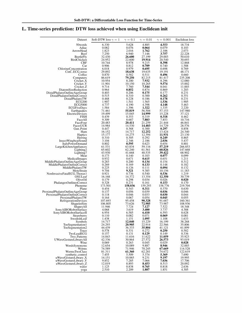
L. Time-series prediction: DTW loss achieved when using Euclidean init

Dataset Soft-DTW loss γ = 1 γ = 0.1 γ = 0.01 γ = 0.001 Euclidean loss

50words 6.330 5.628 4.885 4.553 18.734Adiac 0.082 0.076 0.064 0.079 0.103

ArrowHead 1.823 2.016 1.762 2.106 2.073Beef 7.250 6.940 7.146 3.757 22.228

BeetleFly 32.430 26.600 27.199 29.003 50.610BirdChicken 24.952 22.600 19.914 20.540 30.693

CBF 10.744 8.978 9.215 8.398 12.868Car 0.906 0.812 0.709 0.740 1.588

ChlorineConcentration 6.018 0.979 0.695 0.698 0.769CinC ECG torso 29.892 18.638 19.635 19.191 48.171

Coffee 0.870 0.582 0.511 0.496 0.660Computers 86.619 79.250 82.215 81.417 235.208Cricket X 10.954 8.200 7.932 8.296 12.080Cricket Y 11.901 10.150 10.265 9.574 15.002Cricket Z 9.714 7.760 7.544 8.041 11.003

DiatomSizeReduction 0.964 0.852 0.874 0.869 1.203DistalPhalanxOutlineAgeGroup 0.403 0.206 0.175 0.177 0.231

DistalPhalanxOutlineCorrect 0.515 0.310 0.300 0.262 0.351DistalPhalanxTW 0.468 0.228 0.186 0.178 0.231

ECG200 1.907 1.541 1.565 1.536 1.905ECG5000 4.737 4.190 4.398 4.148 5.463

ECGFiveDays 1.584 1.396 1.322 1.335 2.220Earthquakes 71.461 55.819 56.504 57.153 147.980

ElectricDevices 19.499 15.045 14.999 15.228 37.121FISH 0.439 0.353 0.319 0.318 0.462

FaceAll 9.309 8.687 7.803 7.853 10.716FaceFour 20.483 20.411 21.259 21.444 46.841

FacesUCR 14.984 14.530 14.403 14.729 28.576Gun Point 0.447 0.368 0.300 0.297 0.858

Ham 16.152 14.717 12.252 13.424 24.340Haptics 15.177 14.275 12.394 11.931 23.130Herring 0.310 0.305 0.292 0.249 0.865

InsectWingbeatSound 3.104 2.346 2.186 2.036 5.437ItalyPowerDemand 0.802 0.595 0.623 0.654 0.881

LargeKitchenAppliances 61.531 63.834 59.116 57.219 266.853Lighting2 65.602 62.240 61.561 60.826 147.668Lighting7 43.930 41.668 40.535 39.422 68.902

Meat 0.173 0.140 0.103 0.077 0.099MedicalImages 0.932 0.671 0.615 0.651 1.211

MiddlePhalanxOutlineAgeGroup 0.283 0.200 0.134 0.154 0.312MiddlePhalanxOutlineCorrect 0.269 0.169 0.133 0.148 0.182

MiddlePhalanxTW 0.225 0.126 0.111 0.094 0.132MoteStrain 9.704 9.321 9.385 10.156 11.183

NonInvasiveFatalECG Thorax1 0.921 0.736 0.540 0.536 1.219OSULeaf 16.168 14.372 13.354 12.350 30.739OliveOil 0.179 0.298 0.034 0.026 0.020

PhalangesOutlinesCorrect 0.328 0.231 0.161 0.153 0.170Phoneme 173.501 158.036 159.293 158.776 219.704

Plane 0.454 0.343 0.311 0.370 0.630ProximalPhalanxOutlineAgeGroup 0.137 0.056 0.039 0.036 0.046

ProximalPhalanxOutlineCorrect 0.118 0.046 0.033 0.030 0.044ProximalPhalanxTW 0.164 0.067 0.054 0.045 0.055RefrigerationDevices 107.693 95.458 90.328 91.687 160.361

ShapeletSim 106.805 73.626 72.985 73.987 108.936ShapesAll 11.946 7.724 7.127 7.522 18.348

SonyAIBORobotSurface 4.068 3.619 3.400 3.737 4.388SonyAIBORobotSurfaceII 6.954 6.585 6.410 6.593 8.628

Strawberry 0.110 0.082 0.071 0.069 0.081SwedishLeaf 1.438 1.151 1.095 1.108 1.633

Symbols 14.717 12.040 15.229 16.199 38.268ToeSegmentation1 24.293 20.905 22.914 22.566 35.806ToeSegmentation2 44.439 36.333 35.804 41.121 61.899

Trace 0.578 0.331 0.272 0.250 0.582TwoLeadECG 0.157 0.131 0.129 0.149 0.336Two Patterns 14.843 11.616 11.622 11.059 35.923

UWaveGestureLibraryAll 42.336 30.864 27.572 26.573 93.019Wine 0.069 0.263 0.045 0.029 0.028

WordsSynonyms 12.654 10.089 9.887 8.946 32.003Worms 74.589 71.946 70.245 67.669 114.528

WormsTwoClass 81.311 61.360 62.281 74.672 122.619synthetic control 7.455 5.509 5.374 5.369 7.690

uWaveGestureLibrary X 14.151 10.065 9.231 9.197 19.995uWaveGestureLibrary Y 9.852 7.285 7.066 7.036 17.706uWaveGestureLibrary Z 12.019 8.893 8.453 8.513 20.092

wafer 1.125 0.838 0.765 0.818 2.636yoga 2.510 2.209 1.807 1.851 4.305

Soft-DTW: a Differentiable Loss Function for Time-Series · ebrated dynamic time warping (DTW ... tiable substitution-cost function : Rp pR !R+ which ... (orange, green, purple, in

Documents