SOCIAL NETWORKING AND INDIVIDUAL OUTCOMES: INDIVIDUAL DECISIONS AND MARKET CONTEXT

NET Institute*

www.NETinst.org

Working Paper #05-16

October 2005

Social Networking and Individual Outcomes: Individual Decisions and Market Context

Yannis M. Ioannides Tufts University

Adriaan R. Soetevent

University of Amsterdam and Tinbergen Institute

* The Networks, Electronic Commerce, and Telecommunications (“NET”) Institute, http://www.NETinst.org, is a non-profit institution devoted to research on network industries, electronic commerce, telecommunications, the Internet, “virtual networks” comprised of computers that share the same technical standard or operating system, and on network issues in general.

SOCIAL NETWORKING AND INDIVIDUAL OUTCOMES:

INDIVIDUAL DECISIONS AND MARKET CONTEXT1

Yannis M. Ioannides

Tufts [email protected]

andAdriaan R. Soetevent

University of Amsterdam and Tinbergen [email protected]

Abstract

This paper examines social interactions when social networking is endogenous. It employsa linear-quadratic model that accommodates contextual effects, and endogenous local inter-actions, that is where individuals react to the decisions of their neighbors, and endogenousglobal ones, where individuals react to the mean decision in the economy, both with a lag.Unlike the simple V AR(1) structural model of individual interactions, the planner’s problemhere involves intertemporal optimization and leads to a system of linear difference equationswith expectations. It highlights an asset-like property of socially optimal outcomes in everyperiod which helps characterize the shadow values of connections among agents. Endogenousnetworking is easiest to characterize when individuals choose weights of social attachmentto other agents. It highlights a simultaneity between decisions and patterns of social at-tachment. The paper also poses the inverse social interactions problem, asking whether it ispossible to design a social network whose agents’ decisions will obey an arbitrarily specifiedvariance covariance matrix.

Keywords: Social Interactions, Social Networks, Neighborhood Effects, Endogenous Net-working, Social Intermediation, Econometric Identification, Strong versus Weak Ties, Valueof Social Connections.

JEL classification codes: D85, A14, J0.

Ioannides NET Institute paper.tex September 30, 2005

1Ioannides gratefully acknowledges support by the NET Institute. Soetevent’s research was supported bya grant from the Program of Fellowships for Junior Scholars of the MacArthur Research Network on SocialInteractions and Economic Inequality. Insightful comments by the conference participants, especially AlanKirman, and by Bruce Weinberg on an earlier version have been very helpful. This is a revision of theversion presented at “Networks, Aggregation and Markets,” Conference in honour of Alan Kirman, EHESSand GREQAM–IDEP, Marseille, June 20–21, 2005.

Please address editorial correspondence to Yannis Ioannides.

1 Introduction

Most of the empirical work on social interactions tries to analyze and identify econometricallyinteractions of a mean-field type. This literature typically assumes that individual agents areinfluenced by the average behavior of the social group to which they belong. Such relianceon a broad class of mean field models has shifted attention away from other features of socialinteractions, such as individuals’ deliberate efforts to acquire desirable, or avoid undesirable,social connections. Ioannides and Zabel (2002) explicitly model group membership but thegroups or neighborhoods they specify are non-overlapping and within each neighborhood,mean-field type interactions are assumed. The nascent experimental literature on networkformation (see Kosfeld, 2004, for a survey) is a promising development. These studies focus,however, is on the evolution of networks in rather stylized small scale games.

The present paper differs from other approaches to endogenous group formation by itsemphasis on macroeconomic aspects of network structure associated with the social groupswhich result from individuals’ social networking: their initiatives to link with others. Thepaper investigates the link between social networking and social interactions when patterns ofsocial interactions may be more complex than in the mean field case. If individuals in choosingtheir own actions, which we interpret as incomes, are affected by social interdependence butdo not react strategically to it, individual income outcomes may be restricted with respectto the universe of social outcomes that may reached. Patterns of interdependence may alsoreflect self-selection associated with individuals’ choice of groups.

The particular approach adopted by this paper is in part motivated by the desire to explorein greater depth the notion of social settings where some individuals may be more “influential”than others, and the observation that within groups, subgroups or cliques of agents existwith more intense mutual interaction. A natural question to pose pertains to the potentialfor econometric identification when observational data may be used to make inferences aboutinteraction topology (also referred in the literature as network geography or morphology)along with individuals’ behavioral parameters. A key consequence of social interactions inmodelling social phenomena is that even if individuals are subject to random shocks that areindependent, their individual reactions may end up being stochastically dependent, preciselybecause individual reactions reflect influences from others directly — one’s own actions reflectthose of others — or indirectly, because one’s own actions reflect characteristics of others thatinfluence behavior. Interdependence may also follow from the fact individuals take deliberateefforts to form social groups [ Moffitt (2001) ].

1

When association with others is valuable, it is also appropriate to wonder about existenceof markets through which such “social networking” may be mediated. In fact, networkingmarkets appear to be thriving sometimes and not so much at other times, at least accordingto the popular press; see, for example, Rivlin (2005a; 2005b). Creation of such markets isconceptually related to completing asset markets in an economy, an intuition which could beexplored further in the paper.

The remainder of the paper is organized as follows. The paper first introduces a modelof individual decisions that allows for local and global interactions. The model allows for thefull range of social interactions with continuous outcomes, as they have been formalized bya number of researchers, including notably Bisin et al. (2004), Brock and Durlauf (2001),Glaeser, Sacerdote and Scheinkman (2003), Glaeser and Scheinkman (2001), Manski (1993;2000), Moffitt (2001) and Weinberg (2004) in the economics literature. Our paper is mostnotably related to Weinberg (2004) who introduces utility from social interaction with othersand emphasizes the role of the interaction structure on thresholds and of inputs, like owntime, that an individual may associate with a given set of neighbors. Weinberg shows thatendogeneity of association introduces additional structure that aids identification, thus relax-ing the Manski “social reflection” problem.2 Weinberg also provides empirical results withdata from Add Health from the National Longitudinal Study of Adolescent Health. UnlikeWeinberg, we are also exploring dynamic aspects of social networking Suitable specificationof such interactions makes it possible to express a rich variety of patterns of social interdepen-dence that may have important consequences in the context of the life cycle model as well,along the lines of earlier research by Binder and Pesaran (1998; 2001). Unlike Weinberg butsimilarly to Binder and Pesaran, we are also exploring dynamic aspects of social networking.We go beyond than those authors in obtaining precise analytical results when networkingis endogenous. The paper is conceptually related to the problems addressed by Bala andGoyal (2004) and Goyal and Vega-Redondo (2004) but like Binder and Pesaran, op. cit., andWeinberg, op. cit., uses very different techniques in order to render results that are moreamenable to empirical analysis.

The relationship of this paper to those earlier works will be clarified further below. Weemploy the model first in a static setting, which allows us to explore its implications forinterdependence of individual outcomes in the long run. This development allows us toexamine the “inverse social interactions” problem, that is whether or not an arbitrary social

2This is, in principle, the same effect as the one that endogeneity of neighborhood choice introduces intoeven a linear model [Brock and Durlauf (2001; Durlauf (2004)].

2

outcome, that is one that has been defined as a random vector with a given probabilitydistribution, may be reached as a limit state of social interactions in the long run.

Next the paper turns to investigation of the range of social outcomes that may be reachedwhen individuals choose deliberately how much they wish to be influenced by other individu-als. Conceptually, this is related to choice of social groups or neighborhoods to belong to. Weexplore the literature in neighborhood choice and in formation of friendships in articulatingdifferent possibilities that may result in sorting in terms of observables or of unobservables.We explore similarities between the motivation that individuals have for social networkingand the incentives to fully share risks.

2 Social Setting and Preferences

We employ the concept of social networking in the sense of acquiring access to benefitsthat emanate from activities of other individuals within a particular social setting, or, putdifferently, of acquiring access to desirable and avoiding undesirable social interactions.

We specify a social setting in terms of a social interactions topology. A social interactionsstructure, or topology, is defined in terms of the adjacency matrix Γ [Wasserman and Faust(1994)] of the graph G among i = 1, . . . , N individuals as follows:

γij =

{1 if i and j are neighbors in G;0 otherwise.

(1)

The adjacency matrix will be time-subscripted when appropriate. If social interactions areassumed to be undirected, the adjacency matrix (or sociomatrix) Γ is symmetric. We definean individual i’s neighborhood as the set of other agents she is connected with in the sense ofthe adjacency matrix, j ∈ ν(i), ∀j, Γij = 1. Γi denotes row i of the adjacency matrix, whosenonzero elements correspond to individual i’s neighbors. Further below, it will be importantto allow for a weighted adjacency matrix.

Social interactions may be embedded in a variety of settings, such as consumption activi-ties, human capital accumulation, or more generally income-generating activities. We choosethat last setting and assume that individual i derives utility Uit from an income generatingactivity, income for short, yit in period t net of the (utility) cost of doing so. Utility Uit isassumed to be concave in yit. It also depends on the incomes and the characteristics of i’sneighbors in the sense of the social structure and possibly on the average income in the entireeconomy. Specification of the dependence on income and characteristics of others allows us

3

to express a variety of social interactions, neighborhood and peer effects. We discuss theseafter we introduce notation.

Let

Yt := (y1t, y2t, . . . , yNt)′ denote the (column) vector with elements all individuals’ incomesat time t;

xi : a row K−vector with i’s own characteristics;

X : a N ×K matrix of characteristics for all individuals;

xν(i) : a row K−vector with the mean characteristics of i’s neighbors, j ∈ ν(i), xν(i) =1

|ν(i)|ΓiX;

ι : a row N− vector of ones.

φ, θ, α and ω are column K−vectors of parameters.

We assume individual i at time t enjoys socializing with individuals with specific char-acteristics. This is expressed through taste over the mean characteristics of i’s neighborsj ∈ ν(i), 1

|νt(i)|Γi,tXφ, a level effect. We allow for the marginal utility of own income to de-pend on neighbors’ mean characteristics, which is expressed through the term 1

|νt(i)|Γi,tXθyit,

and separately, on her own characteristics, through a term xiαyit. The former may be referredto as a local contextual effect.

We allow, symmetrically, individual i at time t to be affected by her neighbors’ incomein two ways. One may be thought of as conformism: individual i suffers disutility from agap between her own income and the mean income of her neighbors in the previous period,yit− 1

|νt−1(i)|Γi,tYt−1. A second way allows for the effect of a change in a neighbor’s income todepend on i’s own characteristics through a term 1

|νt(i)|Γi,tYt−1xiω. This allows the effect ofthe neighbors income to depend on individual background characteristics, e.g. younger peoplemay experience a greater disutility from living in a high-income neighborhood. We also allowfor a global conformist effect, through the divergence between an individual’s current incomeand the mean income among all individuals in the previous period, yit − yt−1. This impliesendogenous global interactions.

We assume that each individual i incurs a (utility) cost for maintaining a connection withindividual j at time t is a quadratic function of the “intensity” of the social attachment asmeasured by γij , that is, −c1Γi,tι−c2Γi,tΓ′i,t, with c1, c2 > 0, where ι denotes an N−column

4

vector of 1s.3 This component of the utility function matters when we consider weightedadjacency matrices in section 6.

Finally, we allow for an individual’s own marginal utility to include an additive stochasticshock, εit, which will be discussed in further detail below. Lagging the effect of neighbors’decisions, while keeping the contemporaneous neighborhood structure, is analytically con-venient but not critical. We discuss below in more detail the consequences of includingcontemporaneous effects of neighbors’ decisions.

All these effects are represented in a quadratic utility function, the simplest possiblefunctional form that yields linear first order conditions:4

Uit = Γi,tXφ + (α0 + xiα + Γi,tXθ + εi,t) yit − 12(1− βg − β`)y2

it

− βg

2(yit − yt−1)

2 − β`

2

(yit − 1

|νt(i)|Γi,tYt−1

)2

+1

|νt(i)|Γi,tYt−1xiω − c1Γi,tι− c2Γi,tΓ′i,t. (2)

As we see below, some of these terms do not contribute to individuals’ reaction functions, butdo affect the utility an individual derives from networking with particular other individuals.This allows for social effects in the endogenous social networking process.

Our specification of the utility function nests a number of existing approaches in theliterature, including Durlauf (2004), Glaeser, Sacerdote and Scheinkman (2003), Horst andScheinkman (2004), and Weinberg (2004). Regarding the general formulation of the social in-teractions problem by Binder and Pesaran (1998; 2001), we note the following. First, Binderand Pesaran (2001) assume that the social weights are constant across individuals, whereaswe posit an arbitrary adjacency matrix which may accommodate the full range between localand global interactions. Second, those authors do not examine deliberate social network-ing. Yet, they do provide an exhaustive analysis of solutions of rational expectations modelsfor certain classes of social interactions. They also address the infinite regress problem (offorecasting what the average opinion expects the average opinion to be, etc.) by condition-ing on public information only. Our utility function is analytically quite similar to that in

3When entries of the adjacency matrix are restricted to zero-one values, the total cost to individual i canbe written simply as −(c1 + c2)Γi,tι.

4An additional advantage of quadratic utility functions is that they lend themselves quite easily to formu-lation of decision problems as robust control problems, that is when agents make decisions without knowledgeof the probability model generating the data. See Backus et al. (2004) for a simple presentation and Hansenand Sargent (2005) for a thorough development of robust control as a misspecification problem.

5

ibid. and to Weinberg (2004). By appropriate redefinition of the adjacency matrix it mayaccommodate habit persistence.5 6 It is possible that individuals may differ with respect toattitudes towards conformism or altruism, which would require a more general specificationof preferences than (2).

3 Individual Decision Making

At the beginning of period t, individual i augments her information set Ψit by observing herown preference shock, εit, her neighbors’ actual incomes in period t−1, Γi,tYt−1, and the meanlagged income for the entire economy, yt−1, and chooses an income plan {yit, yit+1, . . . |Ψit },so as to maximize expected lifetime utility conditional on Ψit,

E{∑

s=t

δs−tUi,s |Ψit

}, (3)

where δ, 0 < δ < 1, is the rate of time preference and individual utility is given by (2). Wenote that individual i in choosing her plan recognizes that yit enters Ui,t+1 only if βg 6= 0,

that is only if endogenous global interactions are assumed. That is due to the fact that yit

enters period t + 1 utility functions of all agents j other than agent i, j 6= i. That is, in ourdefinition of the adjacency matrix, γii = 0, and the term Γi,t+1Yt does not contain yit.

7

The first order condition with respect to yit, given the social structure, is:

yit =β`

|νt(i)|Γi,tYt−1 + βgyt−1 + δβg

NE {(yi,t+1 − yt) |Ψit }+ α0 + xiα + Γi,tXθ + εit. (4)

5That is, adopting their assumption would yield quadratic components of the form

1

2(yit − ηyi,t−1)

2 − β

2

(yit − ηyi,t−1 −

(1

|ν(i)|ΓiYt − η1

|ν(i)|ΓiYt−1

))2

,

as in Binder and Pesaran (2001), Equ. (14)), with parameter β > 0 measuring conformism. They modelconformism by expressing a tradeoff between individual-specific growth in consumption, on one hand, andthe gap between that growth and its counterpart among an individual’s neighbors, on the other. They modelaltruism by expressing a tradeoff between the excess of one’s own current income over target lagged incomeand its counterpart among one’s neighbors.

6Following Equ. (15)) in ibid. would yield

−1

2

(yit − ηyi,t−1 + τ

(1

|ν(i)|ΓiYt − η1

|ν(i)|ΓiYt−1

))2

,

with parameter τ > 0 reflecting altruism and τ < 0 reflecting jealousy.7See Bisin, Horst and Ozgur (2004) while assuming only one-sided interactions also allow for a global effect.

6

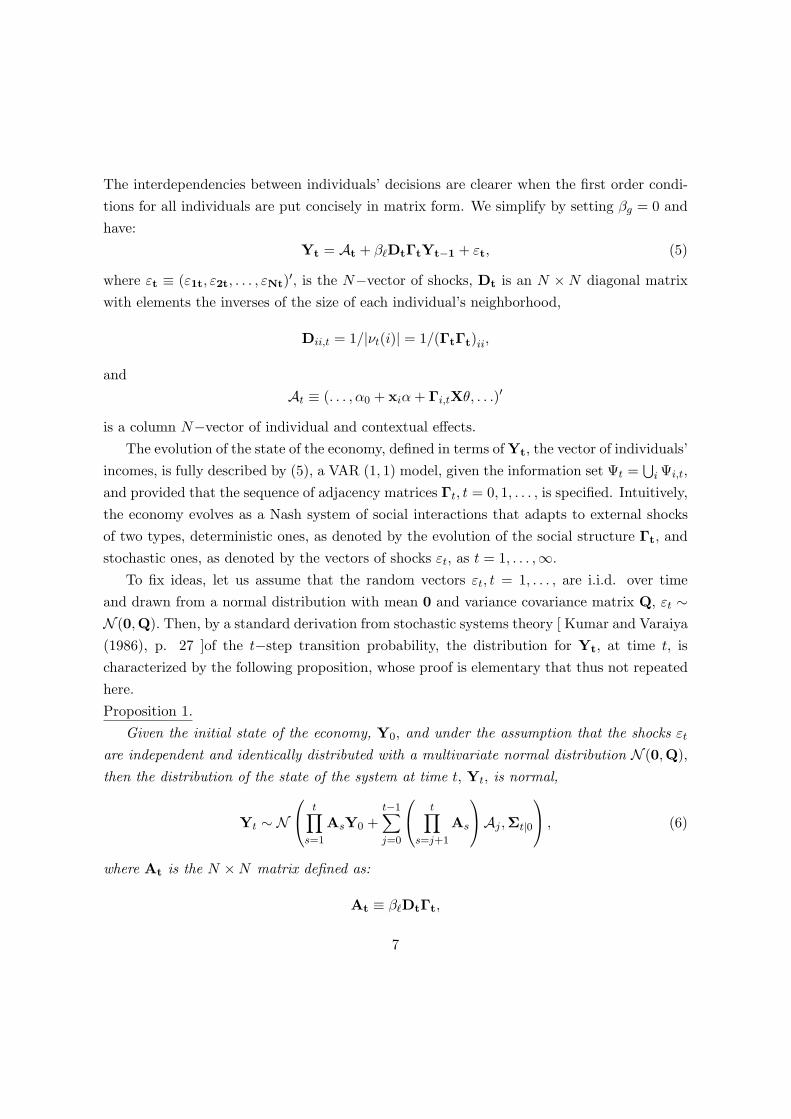
The interdependencies between individuals’ decisions are clearer when the first order condi-tions for all individuals are put concisely in matrix form. We simplify by setting βg = 0 andhave:

Yt = At + β`DtΓtYt−1 + εt, (5)

where εt ≡ (ε1t, ε2t, . . . , εNt)′, is the N−vector of shocks, Dt is an N ×N diagonal matrixwith elements the inverses of the size of each individual’s neighborhood,

Dii,t = 1/|νt(i)| = 1/(ΓtΓt)ii,

andAt ≡ (. . . , α0 + xiα + Γi,tXθ, . . .)′

is a column N−vector of individual and contextual effects.The evolution of the state of the economy, defined in terms of Yt, the vector of individuals’

incomes, is fully described by (5), a VAR (1, 1) model, given the information set Ψt =⋃

i Ψi,t,

and provided that the sequence of adjacency matrices Γt, t = 0, 1, . . . , is specified. Intuitively,the economy evolves as a Nash system of social interactions that adapts to external shocksof two types, deterministic ones, as denoted by the evolution of the social structure Γt, andstochastic ones, as denoted by the vectors of shocks εt, as t = 1, . . . ,∞.

To fix ideas, let us assume that the random vectors εt, t = 1, . . . , are i.i.d. over timeand drawn from a normal distribution with mean 0 and variance covariance matrix Q, εt ∼N (0,Q). Then, by a standard derivation from stochastic systems theory [ Kumar and Varaiya(1986), p. 27 ]of the t−step transition probability, the distribution for Yt, at time t, ischaracterized by the following proposition, whose proof is elementary that thus not repeatedhere.Proposition 1.

Given the initial state of the economy, Y0, and under the assumption that the shocks εt

are independent and identically distributed with a multivariate normal distribution N (0,Q),then the distribution of the state of the system at time t, Yt, is normal,

Yt ∼ N

t∏

s=1

AsY0 +t−1∑

j=0

t∏

s=j+1

As

Aj ,Σt|0

, (6)

where At is the N ×N matrix defined as:

At ≡ β`DtΓt,

7

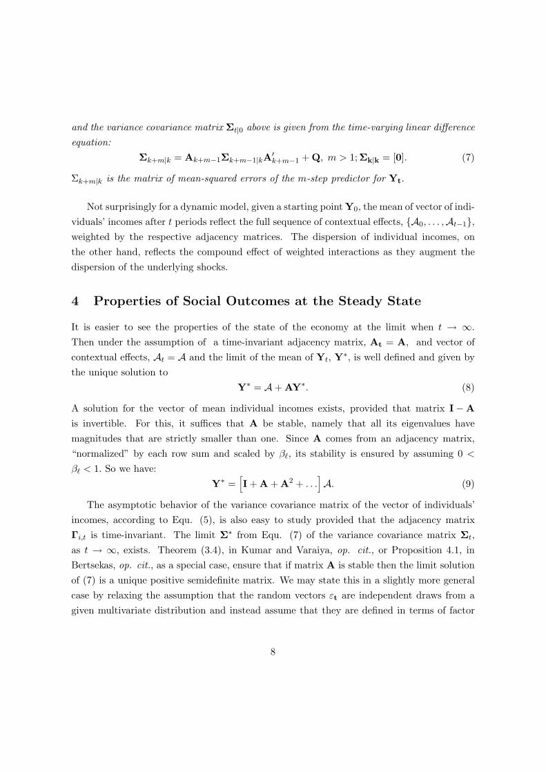
and the variance covariance matrix Σt|0 above is given from the time-varying linear differenceequation:

Σk+m|k = Ak+m−1Σk+m−1|kA′k+m−1 + Q, m > 1;Σk|k = [0]. (7)

Σk+m|k is the matrix of mean-squared errors of the m-step predictor for Yt.

Not surprisingly for a dynamic model, given a starting point Y0, the mean of vector of indi-viduals’ incomes after t periods reflect the full sequence of contextual effects, {A0, . . . ,At−1},weighted by the respective adjacency matrices. The dispersion of individual incomes, onthe other hand, reflects the compound effect of weighted interactions as they augment thedispersion of the underlying shocks.

4 Properties of Social Outcomes at the Steady State

It is easier to see the properties of the state of the economy at the limit when t → ∞.

Then under the assumption of a time-invariant adjacency matrix, At = A, and vector ofcontextual effects, At = A and the limit of the mean of Yt, Y∗, is well defined and given bythe unique solution to

Y∗ = A+ AY∗. (8)

A solution for the vector of mean individual incomes exists, provided that matrix I−A

is invertible. For this, it suffices that A be stable, namely that all its eigenvalues havemagnitudes that are strictly smaller than one. Since A comes from an adjacency matrix,“normalized” by each row sum and scaled by β`, its stability is ensured by assuming 0 <

β` < 1. So we have:Y∗ =

[I + A + A2 + . . .

]A. (9)

The asymptotic behavior of the variance covariance matrix of the vector of individuals’incomes, according to Equ. (5), is also easy to study provided that the adjacency matrixΓi,t is time-invariant. The limit Σ∗ from Equ. (7) of the variance covariance matrix Σt,

as t → ∞, exists. Theorem (3.4), in Kumar and Varaiya, op. cit., or Proposition 4.1, inBertsekas, op. cit., as a special case, ensure that if matrix A is stable then the limit solutionof (7) is a unique positive semidefinite matrix. We may state this in a slightly more generalcase by relaxing the assumption that the random vectors εt are independent draws from agiven multivariate distribution and instead assume that they are defined in terms of factor

8

loadings,εt = Gwt, (10)

where G is an N ×M mixing matrix and wt a random column M−vector, that is indepen-dently and identically distributed over time and obeys a normal distribution with mean 0

and variance covariance matrix R, wt ∼ N (0,R). This case is of particular interest, becauseit allows us to express the contemporaneous stochastic shock in a factor-analytic form ofcontemporaneously interdependent components and therefore shocks to different individualsmay be correlated. This approach also allows for a general form of serial correlation in thewts [ ibid., p. 27 ].8

Put succinctly in a proposition, whose proof readily follows from (7) and (10), we have:Proposition 2.

The variance covariance matrix of vector of individuals’ incomes when t →∞, that is thelimit of (7) when εt assumes the factor-analytic form according to (10), satisfies

Σ∞ = AΣ∞A′ + GRG′. (11)

The matrix Σ∞ in the equation above would not be a proper variance covariance matrixunless it is positive definite. This is ensured, provided the random error wt along with thematrix A “allow” the economy to reach all social outcomes in a well-defined sense. Clarifyingthis involves the concept of controllability, according to which a pair of matrices A,G arecontrollable, if the matrix [G, AG, . . . ,AN−1G] with N rows and NM columns has rankN , that is all its rows are fully independent.Proposition 3. If the pair of matrices A,G is controllable, then stability of matrix A isequivalent to existence of a unique solution to Equ. (11) that is positive definite and viceversa.

Proof. Matrix A is indeed stable, as we discussed earlier above. Then, Theorem (3.9), inKumar and Varaiya, op. cit., applies. Alternatively, by applying Equ. (11) recursively wehave that if limt→∞AtGRG′(A′)t = [0], then

Σ∞ =∞∑

j=0

AjGRG′(A′)j .

8Such a factor-analytic approach links social interaction models with factor models in large cross-sectionsof time series that have been employed in generalizing the dynamic index models of business cycle research.See Reichlin (2002) for an excellent review of this recent literature.

9

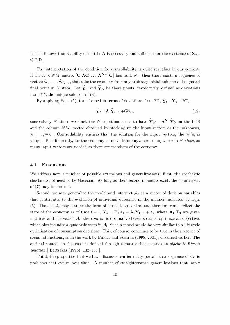
It then follows that stability of matrix A is necessary and sufficient for the existence of Σ∞.

Q.E.D.

The interpretation of the condition for controllability is quite revealing in our context.If the N × NM matrix [G|AG| . . . |AN−1G] has rank N , then there exists a sequence ofvectors

∼w0, . . . ,

∼wN−1, that take the economy from any arbitrary initial point to a designated

final point in N steps. Let∼Y0 and

∼YN be these points, respectively, defined as deviations

from Y∗, the unique solution of (8).By applying Equ. (5), transformed in terms of deviations from Y∗,

∼Yt≡ Yt −Y∗,

∼Yt= A

∼Yt−1 +Gwt, (12)

successively N times we stack the N equations so as to have∼YN −AN

∼Y0 on the LHS

and the column NM−vector obtained by stacking up the input vectors as the unknowns,∼w0, . . . ,

∼wN . Controllability ensures that the solution for the input vectors, the

∼wt’s, is

unique. Put differently, for the economy to move from anywhere to anywhere in N steps, asmany input vectors are needed as there are members of the economy.

4.1 Extensions

We address next a number of possible extensions and generalizations. First, the stochasticshocks do not need to be Gaussian. As long as their second moments exist, the counterpartof (7) may be derived.

Second, we may generalize the model and interpret At as a vector of decision variablesthat contributes to the evolution of individual outcomes in the manner indicated by Equ.(5). That is, At may assume the form of closed-loop control and therefore could reflect thestate of the economy as of time t − 1, Yt = BtAt + AtYt−1 + εt, where At,Bt are givenmatrices and the vector At, the control, is optimally chosen so as to optimize an objective,which also includes a quadratic term in At. Such a model would be very similar to a life cycleoptimization of consumption decisions. This, of course, continues to be true in the presence ofsocial interactions, as in the work by Binder and Pesaran (1998; 2001), discussed earlier. Theoptimal control, in this case, is defined through a matrix that satisfies an algebraic Riccatiequation [ Bertsekas (1995), 132–133 ].

Third, the properties that we have discussed earlier really pertain to a sequence of staticproblems that evolve over time. A number of straightforward generalizations that imply

10

intertemporal tradeoffs can render the model genuinely dynamic. The simplest possible one,as we discussed above, would be to allow for a global effect, that is by allowing βg 6= 0.

Fourth, an interesting extension would be to allow for the stochastic shocks to be decisionvariables. The simplest way to do so would be via endogenizing the factor loadings, that isby letting individuals set the elements of the mixing matrix in Equ. (10), G, which couldalso be time-varying. This would then resemble a dynamic portfolio analysis problem, whichwe know to be quite tractable when individuals’ utility functions are quadratic. We notethe special interpretation that the choice of a portfolio of factors would confer: individualschoose factor loadings in order to offset shocks associated with the decisions of others thatenter directly their own utility functions and therefore their own decisions as well.

Fifth, suppose that an arbitrarily chosen state of the economy may be specified via arandom N−vector Y, with a given distribution function, Y ∼ N (F, ς). That is, the incomesof the individual members of the economy are assumed to be stochastically interdependentand distributed in the above fashion. We define the inverse social interactions problem aswhether such a state could be reached as an outcome of social interactions, that is as thelimit vector of individuals’ incomes, satisfying (5), when t → ∞. That is, given (F, ς) andthe distributional characteristics of the random vector of factors wt, wt ∼ N (0,R), can wefind a social interactions structure, defined by a vector of coefficients A, an adjacency matrixΓ, and a mixing matrix G of dimension N ×M, such that the random vector Y is the limit,when t →∞, of the vector of individual outcomes, Yt,

Yt = A+ AYt−1 + Gwt. (13)

The inverse social interactions problem is the counterpart here of problems posed by thebusiness cycle literature, that is whether it might be possible to define vector autoregressivesystem that yields any desirable pattern of correlations among the shocks [Jovanovic (1987);Sargent (1987)]. We note that this problem is more general than examining the limit of thedistribution of income in this economy.

First we note that given F, (13) implies that F = [I −A]−1A. If a mixing matrix G isgiven, then we may define the square root S of GRG′, SS′ = GRG′. The problem of findinga positive symmetric matrix of full rank N , A, is overdetermined: there exist 1

2N(N +1)+N

equations and 12N(N − 1) unknowns. Therefore, there exist up to 2N degrees of freedom

which may be used for the determination of the mixing matrix.This result is readily interpretable in terms of weighted adjacency matrices. Imposing

the restriction that the social interaction matrix takes the form of a matrix of zeros and

11

ones, with A = βDΓ, translates to the requirement that given ς, a matrix Γ and a socialinteractions coefficient β may be found that provide sufficient spanning for ς to be the limitdistribution satisfying Equ. (11). Relaxing the requirement would be to allow for individuals’interaction coefficients to differ, (β1, . . . , βN ), or alternatively, for the adjacency matrix toassume a weighted form with arbitrary positive entries, instead of just 0s and 1s. The caseof a weighted adjacency matrix is taken up further below in section 6.

5 A Social Planner’s Problem

Next we introduce a social planner who recognizes the interdependence of agents and alsotakes it into consideration in setting individuals’ outcomes while respecting an existing topol-ogy of social interactions. This analysis helps assess the scope for social intermediation, aswe shall see shortly below.

The planner seeks to choose individuals’ incomes that maximize the sum of individuals’expected lifetimes utilities.9 The planner is forward-looking and in recognizing individuals’interdependence she conditions her decisions on knowledge of all incomes in the previousperiods, {Y0,Y1, . . . ,Yt−1}, and of all individual preference information available as of thebeginning of every time period, Ψt. At the beginning of each period t, the planner choosesa plan {Yt,Yt+1, . . . , } so as to maximize the expectation of individuals’ lifetime utility,according to

N∑

i=1

Uit + E

∑

s=t+1

δs−tUi,s|Ψt

. (14)

The planner’s maximization assumes actual outcomes as of time period t and the exogenousevolution of the adjacency matrix Γt, and where we have also simplified utility function (2)by assuming that βg = 0, ω = 0.

Differentiating objective function (14) with respect to yit, i = 1, . . . , N, yields the firstorder conditions:

yit + δβ`

∑

j 6=i

γji,t+1

|νt+1(j)|1

|νt+1(j)|Γj,t+1Yt

=β`

|νt+1(i)|ΓitYt−1 + δβ`

∑

j 6=i

γji,t+1

|νt+1(j)|E {yj,t+1|t}+Ait + Giwt. (15)

9We eschew introduction of arbitrary positive weights λ1, . . . , λN , because they are not really necessary forexpressing the planner’s problem. There are sufficient degrees of freedom elsewhere in the individuals’ utilityfunctions.

12

We may rewrite these conditions for all i’s in matrix form as follows:

[I + δβ`Γ′t+1Dt+1Dt+1Γt+1

]Yt

= At + β`Dt+1ΓtYt−1 + δβ`Γ′t+1Dt+1 E {Yt+1|Ψt}+ Gwt. (16)

By working in the standard fashion for linear-quadratic rational expectations models, wesolve for Yt as a function of Yt−1 and of E {Yt+1|t} . Specifically, we simplify by assumingthat the adjacency matrix and the matrix of contextual effects are time invariant, and define:

H = I + δβ`Γ′DDΓ

Then solving Equ. (16) yields:

Yt = H−1 [A+ β`DΓYt−1 + δβ`Γ′D E {Yt+1|Ψt}+ Gwt]. (17)

By advancing the time subscript, taking expectations and using the law of iterated expec-tations, we may express E {Yt+1|Ψt} in terms of Yt and E {Yt+2|Ψt} , and so on. Thatis:

E {Yt+1|t} = H−1 [A+ β`DΓYt + δβ`Γ′D E {Yt+2|t}].

By iterating forwards from time t + 1, we obtain the standard form of the forward solutionfor systems of linear rational expectations models. Put concisely in the form of a propositionwe have:Proposition 4.

Part A. Maximization of expected social welfare, defined as the sum of expected life timeutilities of all agents requires that the vector of outcomes Yt satisfies the system of lineardifference equations (16) with expectations.

Part B. The expectation of the vector of optimal outcomes at the steady state, when allcovariates are time-invariant, Y∗, satisfies

E{Y∗

}= A+ β`DΓE

{Y∗

}+ δβ`Γ′D [I−DΓ] E

{Y∗

}, (18)

and is well defined and unique.The economic interpretation of Equ. (18) is straightforward. At the steady state, the

vector of expected outcomes is equal to the vector of contextual effects, of the own laggedfeedbacks, and of the net “conformist” effect on one’s neighbors in the following period.Precise results regarding the properties of the solution to the above model may be obtained

13

by applying Proposition 3, Binder and Pesaran (1998). We plan to return to this issue in alater version of the paper. We do note that a richer behavioral model than the one in Section3, while possible and attractive, would have complicated considerably the use we make of ourbehavioral model later on in the paper.

A number of remarks are in order. First, systems of linear difference equations withexpectations, like (16), have been studied extensively and are amenable to solution in thestandard fashion for such models [Sargent (1987); Binder and Pesaran, op. cit.]. Expectationsenter because the planner recognizes that setting individual i’s period t outcome affects theexpectation of the utilities of her neighbors in the following period. In contrast, individuals’optimization considerations are backward looking, and therefore the first-order conditionsyield a simple vector autoregression of order 1.

Second, by employing the methods used earlier and summarized in Proposition 1 above,it is possible to extend Proposition 4 so as to clarify the evolution of the variance-covariancematrix for the socially optimal outcomes vector.

Third, iterating Equ. (17) forwards demonstrates an asset-like property of socially optimalperiod t outcomes, Yt. That is, the value from setting an individual’s outcome in this perioddepends upon others’ outcomes next period, and so on. This confers an element of asset toagents’ outcomes and leads to an asset theory of social interactions. At the social optimum,individual outcomes at time t reflect the present value of the future stream of contextualeffects of all current neighbors, adjusted by discount factors that are functions of the rateof time preference and multiplied by the social interactions coefficient and weighted by thedirectness of the connections between agents. It is not surprising that the planner is forwardlooking in assessing the effects that different individuals’ actions have on their own outcomesand those of their neighbors. The one period forward dependence is, of course, translatedinto the standard infinitely forward dependence familiar from rational expectations models.

Fourth, we note that there is another aspect of the social value of social interactions whichthe effect discussed above does not capture. That is, the value for an agent of having versusnot having a particular connection with another agent. Associated with every solution path isan expected value of the social welfare function, the planner’s objective function. Therefore,in principle, we may assess the impact of a change in the adjacency matrix on the sociallyoptimal solution and thus on the expected value of the planner’s objective function. That is,adding a new link changes the solution path in a particular way and produces an increment inthe expected value of the planner’s objective function. In general, this yields a shadow value

14

for the corresponding link which is a benchmark by means of which we may measure thesocial value of intermediation. This calculation is straightforward conceptually. In practice,it is quite tedious to compute the social value of an additional connection.

Since the individually optimal outcomes are inefficient, the social optimum may be imple-mented, at least conceptually, through an appropriately chosen set of prices, πit, i = 1, . . . , N.

By adapting individual i’s utility so as to include a term −πityit, maximization of Uit−πityit

brings about the social optimum, provided that the prices are set equal to the respectivemarginal social effects, which in view of quadratic utility functions are equal to the differ-ence between the socially optimal and individually optimal outcomes. For completeness, wealso need to impose conditions of incentive compatibility and allow for transfers that leaveindividuals at least indifferent while budget balance is satisfied.

So far we have assumed that the network of social connections is given. We next turn tothe situation where this network is endogenous. In that case, implementing individual pricesπit in general is insufficient as a tool for the social planner to implement the social optimumof outcomes and network connections.

6 Endogenous Networking

How could social network connections come about? This section explores the notion thatthey are initiated by means of individuals’ initiatives, when individuals stand to benefit bydoing so. We examine endogenous networking by assuming that individuals choose weightswhich they associate with their connections with other individuals. This approach assuagesthe inherent difficulty of dealing with discrete endogenous variables while taking advantageof a natural interpretation of weighted social connections. Individuals’ social attachmentsdo differ: they vary from close friendships to mere acquaintances. And, naturally, weightedadjacency matrices are used in the social science literature. A formulation of endogenousnetworking in a discrete setting of the model of social connections we have been working withso far is relegated to an appendix in a working paper version of the paper. It demonstratesthat characterization of individual networking initiatives is quite awkward, and so is theassociated welfare analysis.

Analysis of endogenous networking is facilitated by assuming a finite horizon, T, versionof the typical individual’s problem and considering the networking decision prior to setting

15

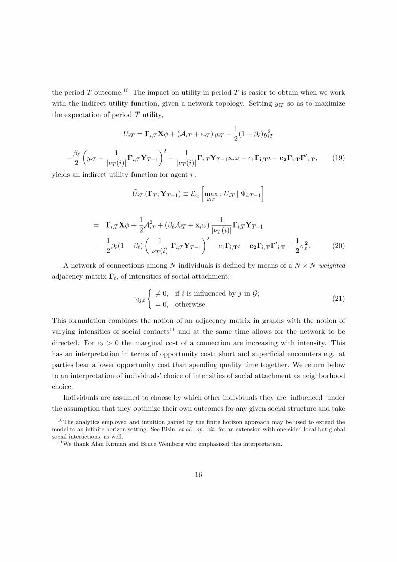
the period T outcome.10 The impact on utility in period T is easier to obtain when we workwith the indirect utility function, given a network topology. Setting yiT so as to maximizethe expectation of period T utility,

UiT = Γi,TXφ + (AiT + εiT ) yiT − 12(1− β`)y2

iT

−β`

2

(yiT − 1

|νT (i)|Γi,TYT−1

)2

+1

|νT (i)|Γi,TYT−1xiω − c1Γi,Tι− c2Γi,TΓ′i,T, (19)

yields an indirect utility function for agent i :

UiT (ΓT ;YT−1) ≡ Eεt

[maxyiT

: UiT | Ψi,T−1

]

= Γi,TXφ +12A2

iT + (β`AiT + xiω)1

|νT (i)|Γi,TYT−1

− 12β`(1− β`)

(1

|νT (i)|Γi,TYT−1

)2

− c1Γi,Tι− c2Γi,TΓ′i,T +12

σ2ε . (20)

A network of connections among N individuals is defined by means of a N ×N weightedadjacency matrix Γt, of intensities of social attachment:

γij,t

{6= 0, if i is influenced by j in G;= 0, otherwise.

(21)

This formulation combines the notion of an adjacency matrix in graphs with the notion ofvarying intensities of social contacts11 and at the same time allows for the network to bedirected. For c2 > 0 the marginal cost of a connection are increasing with intensity. Thishas an interpretation in terms of opportunity cost: short and superficial encounters e.g. atparties bear a lower opportunity cost than spending quality time together. We return belowto an interpretation of individuals’ choice of intensities of social attachment as neighborhoodchoice.

Individuals are assumed to choose by which other individuals they are influenced underthe assumption that they optimize their own outcomes for any given social structure and take

10The analytics employed and intuition gained by the finite horizon approach may be used to extend themodel to an infinite horizon setting. See Bisin, et al., op. cit. for an extension with one-sided local but globalsocial interactions, as well.

11We thank Alan Kirman and Bruce Weinberg who emphasized this interpretation.

16

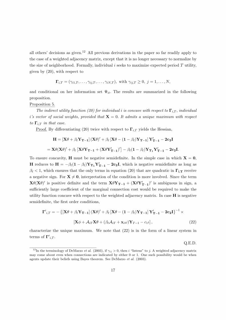
all others’ decisions as given.12 All previous derivations in the paper so far readily apply tothe case of a weighted adjacency matrix, except that it is no longer necessary to normalize bythe size of neighborhood. Formally, individual i seeks to maximize expected period T utility,given by (20), with respect to

Γi,T = (γi1,T , . . . , γij,T , . . . , γiN,T ), with γij,T ≥ 0, j = 1, . . . , N,

and conditional on her information set Ψit. The results are summarized in the followingproposition.Proposition 5.

The indirect utility function (20) for individual i is concave with respect to Γi,T , individuali’s vector of social weights, provided that X = 0. It admits a unique maximum with respectto Γi,T in that case.

Proof. By differentiating (20) twice with respect to Γi,T yields the Hessian,

H = [Xθ + β`YT−1] (Xθ)′ + β` [Xθ − (1− β`)YT−1]Y′T−1 − 2c2I

= Xθ(Xθ)′ + β`

[XθYT−1 + (XθY′

T−1)′]− β`(1− β`)YT1Y

′T−1 − 2c2I.

To ensure concavity, H must be negative semidefinite. In the simple case in which X = 0,H reduces to H = −β`(1 − β`)YT1Y

′T−1 − 2c2I, which is negative semidefinite as long as

β` < 1, which ensures that the only terms in equation (20) that are quadratic in Γi,T receivea negative sign. For X 6= 0, interpretation of the condition is more involved. Since the termXθ(Xθ)′ is positive definite and the term XθYT−1 + (XθY′

T−1)′ is ambiguous in sign, asufficiently large coefficient of the marginal connection cost would be required to make theutility function concave with respect to the weighted adjacency matrix. In case H is negativesemidefinite, the first order conditions,

Γ′i,T = − {[Xθ + β`YT−1] (Xθ)′ + β` [Xθ − (1− β`)YT−1]Y′

T−1 − 2c2I}−1×

[Xφ +AiTXθ + (β`AiT + xiω)YT−1 − c1ι] , (22)

characterize the unique maximum. We note that (22) is in the form of a linear system interms of Γ′i,T .

Q.E.D.12In the terminology of DeMarzo et al. (2003), if γij > 0, then i “listens” to j. A weighted adjacency matrix

may come about even when connections are indicated by either 0 or 1. One such possibility would be whenagents update their beliefs using Bayes theorem. See DeMarzo et al. (2003).

17

A number of remarks are in order. First, for certain applications, it may be importantto require the entries of the adjacency matrix to be positive and normalized. RestrictingΓi,T so that it lies in the positive orthant of RN , γij,T ≥ 0, j = 1, . . . , N, a convex set, isstraightforward but quite stringent. That is, that would translate to restrictions on values ofparameters and of variables. While some of the variables are constant, others depend on theactual state of the economy as of the preceding period, YT−1. These values accumulate pastvalues of stochastic shocks and are therefore random. Consequently, endogenous weightednetworking implies that agents in setting their period T − 1 decisions must take into con-sideration that ΓT , the social adjacency matrix in period T, is an outcome of individuals’uncoordinated decisions and stochastic. We note that positivity of the γij,T s is quite criti-cal for a meaningful interpretation of endogenous networking as being akin to neighborhoodchoice. If the adjacency matrix were to be restricted to be positive, then particular patternsin Γ, like a block-diagonal structure with many small blocks is reminiscent of so-called “smallworlds,” emerging endogenously.

Second, endogenous determination of the social adjacency matrix introduces intertempo-ral linkages in the individual’s decision making for two reasons: first, period T − 1 decisionsaffect the period T adjacency matrix ΓT ; and second, unlike when the adjacency matrixwas taken as given and the assumption was made that all diagonal terms were assumed to beequal to zero, γii,t = 0, now they may well be nonzero, thereby strengthening habit formation.From a psychological perspective, one can argue whether positive γii,t’s should be interpretedas the result of willful acts or are expressing addiction. This intertemporal linkage in turnleads to a clarification of the asset value of a connection between agents. Because of ourfunctional specification for individual utility according to Equ. (2), additional information,in the form of total and marginal contextual effects, is brought to bear upon the problemof determining the social structure and also enters the asset value of social connections. Inparticular, additional information is included, over and above information included in thereaction function, such as the term Xφ. Third, once the connection weights are endogenized,weights are not necessarily equal, that is the adjacency matrix is not symmetric, let aloneconstant over time.

We refrain from pursuing further these issues in the present paper. However, in animportant sense, networking, once it has been endogenized no longer implies that socialinteractions assume the form of the mean field case. Furthermore, variable intensities ofattachment subsume the issue of strong versus weak ties [Grannovetter (1994)] as a special

18

case.

6.1 Endogenous Networking and Individual Decisions

In obtaining the first-order conditions for individual i’s decision in period T − 1 we need torecognize that γii,T , which is optimally chosen and satisfies (22) above, need not be equal tozero. Therefore yi,T−1 enters period T indirect utility UiT via the term Γi,TYT−1.

13 Therefore,we now have for all yi,T−1 in matrix form:

[δβ`(1− β`)[DiagΓT]ΓT + I]YT−1 = δ[DiagΓT][β`AT + Xω] + β`ΓT−1YT−2 +AT−1 + εT−1.

(23)where [DiagΓT] denotes the diagonal matrix made up of the diagonal terms of ΓT.

Not surprisingly, the strength of the effect depends on δγii,T . This weighs the own periodT individual and contextual effects Ai,T and the own endogenous local interaction effecton period T utility, as they are added to the period T − 1 individual and contextual effects,Ai,T−1. It also weighs the own conformist effect of the current decision yi,T−1 on itself throughits presence in period T utility.

Finally, we turn to the joint evolution of individual decisions and the social network. Wenote that the setting of YT−1 and ΓT are based on the same information. Therefore, (23) and(22) may be treated as a simultaneous system of equations: period T −1 individual decisionsand period T weights of social attachment are jointly determined. These equations may berewritten schematically as:

ΓT = G (ΓT ,YT−1|X) ,

YT−1 = Y (ΓT ,YT−1,YT−2, εT−1|X) .(24)

The above system of equations is autonomous with only a contemporaneous stochastic shock,the vector εT−1. It exhibits complicated dynamic dependence: it is second-order with re-spect to YT−1 and first-order with respect to ΓT . It is amenable to the usual treatmentfor dynamical systems, but the fact that ΓT is a matrix makes matters cumbersome. Oneespecially has to ensure that the system is dynamically stable, perhaps by imposing a kindof transversality condition that restricts the absolute value of entries in the Γ matrix. Weplan to pursue further the properties of this system in future research.

13It also enters indirectly through the dependence of the endogenous Γi,T on YT−1, but by the envelopetheorem, those terms cancel out.

19

6.2 Comparison with Exogenous Networking

As a contrast to exogenous networking, consider a stylized exogenous networking settingwhere individuals engage in social networking by progressively connecting with the acquain-tances of their acquaintances, and so on. Tracking the evolving acquaintance sets is quitestraightforward [ Brueckner and Smyrnov (2004) ]. Starting with an adjacency matrix Γ0,

it is straightforward to see that all individuals acquire connections with their second neigh-bors, that is the acquaintances of their acquaintances, then the adjacency matrix becomesΓ1 = Γ0 + Γ2

0. Extending to third neighbors (graph-distance three), the adjacency matrixbecomes Γ2 = Γ1 + (Γ1)2 = Γ0 + 2Γ2

0 + 2Γ30 + Γ4

0. Endogenous networking as examinedearlier would lead only by chance to such a description of the evolution of networking at theaggregate. Brueckner and Smyrnov (2004) derive a number of results for the case in whichΓ0 is irreducible, that is, in networks in which every agent is directly or indirectly connectedto every other agent. Notwithstanding the tractability of the network evolution process, onedrawback of this approach is that it is hard to come up with an economic justification of thisparticular evolution process.

7 Conclusions

We conclude by first providing a brief summary. This paper examines social interactionswhen social networking may be endogenous. It employs a linear-quadratic model that ac-commodates contextual effects and endogenous interactions, that is local ones where indi-viduals react to the decisions of their neighbors, and global ones, where individuals reactto the mean decision in the economy, both with a lag. Unlike the simple V AR(1) form ofthe structural model, the planner’s problem involves intertemporal optimization and leadsto a system of linear difference equations with expectations. It also highlights an asset-likeproperty of socially optimal outcomes in every period which helps characterize the shadowvalues of connections among agents. Endogenous networking is easiest to characterize whenindividuals choose weights of social attachment to other agents. It is much harder to do sowhen networking is discrete. The paper also poses the inverse social interactions problem,that is whether it is possible to design a social network whose agents’ decisions will obey anarbitrarily specified variance covariance matrix.

We would like to think of this paper as addressing problems that pursue further the logicof one of Alan Kirman’s greatest contributions. That is, to further study economies with

20

interacting agents in ways that help bridge an apparent gap with mainstream economics[Kirman (1997; 2003)]. Although the paper does not deal with another of Kirman’s keyareas of interest, aggregation, it hopes to contribute indirectly in the following fashion. First,aggregation that ignores the presence of social interactions is a tricky venture [c.f. Kirman(1992)]. Second, social interactions give rise to a social multiplier, construed here in the senseof Glaeser, Sacerdote and Scheinkman (2003). That is, social multiplier is defined as the ratioof the coefficient of a contextual effect obtained from a regression with aggregate data to thatobtained from a regression with individual data. As a consequence of aggregation, the socialmultiplier overstates individual effects, in varying degrees that depend on precise patternsof interdependence and sorting in the data. The tools developed in this paper allows us toexplore the following hypothesis. Might the social multiplier be due to the exogeneity ofsocial interactions as assumed by earlier papers? We know from ibid. that sorting acrossgroups on the basis of observables reduces the social multiplier, but sorting on unbservableshas an ambiguous effect. Our model involves both effects, by positing what is essentially anoptimal “social” portfolio problem. Endogenous social networking makes the case forcefullythat non-market interactions need not be of the mean field type.

In a mechanical sense, our model represents endogeneity of the infrastructure of trade.Dependence on neighbors’ income could be a reduced form for the benefits derived fromtrading with others. In our model, agents are vying to choose a desirable set of others tobe influenced from. We would like to think of this as a precursor to opening up routes fortrading. That is a much harder problem, but one that promises attractive payoffs. Whenmarkets are incomplete, opening up new markets is a tricky business from the viewpoint ofsocial welfare [Newbery and Stiglitz (1984)]. An alternative interpretation of the model is interms of endogenous group formation, and could be pursued further. Therefore, for severalreasons the type of phenomena that Alan Kirman has chosen to emphasize throughout hiswork are central to making economics more relevant and a better tool for understanding howsocieties function.

8 Bibliography

Backus, David, Bryan Routledge, and Stanley Zin (2004), “Exotic Preferences for Macroe-conomists,” NBER Macroeconomics Annual, MIT Press, Cambridge.

Bala, Venkatesh, and Sanjeev Goyal (2000), “A Noncooperative Model of Network Forma-

21

tion,” Econometrica, 68, 5, 1181–1229.

Bertsekas, Dimitri P. (1972), “Infinite-Time Reachability of State-Space Regions by UsingFeeedback Control,” IEEE Transactions in Automatic Control, AC–17, 5, 604–613.

Bertsekas, Dimitri P. (1995), Dynamic Programming and Stochastic Control, Volume 1,Athena Scientific, Belmont, MA.

Binder, Michael, and M. Hashem Pesaran (1998), “Decision Making in the Presence ofHeterogeneous Information and Social Interactions,” International Economic Review,39, 4, 1027–1052.

Binder, Michael, and M. Hashem Pesaran (2001), “Life-cycle Consumption under SocialInteractions,” Journal of Economic Dynamics and Control, 25, 35–83.

Bisin, Alberto, Ulrich Horst, and Onur Ozgur et al. (2004), “Rational Expectations Equilib-ria of Economies with Local Interactions,” Journal of Economic Theory, forthcoming.

Brock, William A., and Steven N. Durlauf (2001) “Interactions-Based Models,” 3297–3380,in Heckman, James J., and Edward Leamer, eds., Handbook of Econometrics, Volume5, North-Holland, Amsterdam.

Brueckner, Jan K. and Oleg Smyrnov (2004), “Workings of the Melting Pot: Social Networksand the Evolution of Population Attributes,” CESifo working paper No. 1320, October.

Calvo-Armengol, Antoni, and Matthew O. Jackson (2004), “The Effects of Social Networkson Employment and Inequality,” American Economic Review, 94, 3, 426–454.

DeMarzo, Peter M., Dimitri Vayanos, and Jeffrey Zwiebel (2003), “Persuasion Bias, SocialInfluence, and Unidimensional Opinions, Quarterly Journal of Economics, CXVIII, 3,909–968.

Durlauf, Steven N. (2004), “Neighborhood Effects,” Ch. 50, in J. Vernon Henderson andJacques-Francois Thisse, eds., Handbook of Regional and Urban Economics: Vol. 4,Cities and Geography, North-Holland, 2004, 2173–2234.

Glaeser, Edward L., Bruce I. Sacerdote and Jose A. Scheinkman (2003), “The Social Mul-tiplier,” Journal of the European Economic Association, 1, 2–3, 345–353.

22

Glaeser, Edward L., and Jose A. Scheinkman (2001), ”Non-market Interactions,” workingpaper; presented at the World Congress of the Econometric Society, Seattle, 2000.

Goyal, Sanjeev, and Fernando Vega-Redondo (2004), “Structural Holes in Social Networks,”working paper, University of Essex, December.

Gronovetter, Mark (1994), Getting a Job: A Study of Contacts and Careers, 2nd edition,Harvard university Press, Cambridge, MA.

Hansen, Lars P., and Thomas Sargent (2005), Misspecification in Recursive MacroeconomicTheory, University of Chicago and the Hoover Institution, manuscript.

Horst, Ulrich, and Jose A. Scheinkman (2004), “Equilibria in Systems of Social Interactions,”Journal of Economic Theory, forthcoming.

Ioannides, Yannis M. (2004), “Random Graphs and Social Networks: an Economics Per-spective,” presented at the IUI Conference on Business and Social Networks, Vaxholm,Sweden, June.

Ioannides, Yannis M., and Linda Datcher Loury (2004), “Job Information Networks, Neigh-borhood Effects, and Inequality,” Journal of Economic Literature, XLII, December,1056–1093.

Ioannides, Yannis M., and Jeffrey E. Zabel (2002), “Interactions, Neighborhood Selectionand Housing Demand,” Tufts working paper 2002-08; revised March 2004.

Jackson, Matthew O., and Asher Wolinsky (1996), “A Strategic Model of Social and Eco-nomic Networks,” Journal of Economic Theory, 71, 44–74.

Jovanovic, Boyan (1987), “Micro Shocks and Aggregate Risk,” The Quarterly Journal ofEconomics, 102, 2, 395–410.

Kirman, Alan P. (1992), “Whom or What Does the Representative Individual Represent?”Journal of Economic Perspectives, 6, 2, 117-136.

Kirman, Alan P. (1997), “The Economy as an Interactive System,” 491–531, in Arthur,W. Brian, Steven N. Durlauf and David A. lane, eds., The Economy as an EvolvingComplex System II, Addison-Wesley, Reading, MA.

23

Kirman, Alan P. (2003), “Economic Networks,” 273–294, in Bornholdt, S., and H. G. Schus-ter, eds., Handbook of Graphs and Networks: From the Genome to the Internet, Wiley- VCH, Weinheim.

Kosfeld, Michael (2004), “Economic Networks in the Laboratory: A Survey,” working paper,Institute for Empirical Research in Economics, University of Zurich.

Kumar, P. R., and P. Varaiya (1986) Stochastic Systems: Estimation, Identification andAdaptive Control, Prentice Hall, Englewood Cliffs, N. J.

Manski, Charles F. (1993), “Identification of Endogenous Social Effects: The ReflectionProblem,” Review of Economic Studies, 60, 531–542.

Moffitt, Robert A. (2001) “Policy Interventions, Low-Level Equilibria and Social Interac-tions,” in Durlauf, Steven N., and H. Peyton Young, eds., Social Dynamics, MIT Press,45–82.

Newman, Mark E. J. (2003), “The Structure and Function of Networks,” SIAM Review, 45,167–256.

Newbery, David M. G., and Joseph E. Stiglitz (1984), “Pareto Inferior Trade,” Review ofEconomic Studies, 51, 1, 1–12.

Reichlin, Lucrezia (2002), “Factor Models in Large Cross-Sections of Time Series,” presentedat World Congress of the Econometric Society, Seattle, 2000; working paper, ECARES,Universite Libre de Bruxelles.

Rivlin, Gary (2005a), “Friendster, Love and Money,” New York Times, January 24.

Rivlin, Gary (2005b), “Skeptics Take Another Look at Social Sites,” New York Times, May9.

Sargent, Thomas J. (1987), Macroeconomic Theory, 2nd edition Academic Press.

Wasserman, Stanley, and Katherine Faust (1994), Social Network Analysis: Methods andApplications, Cambridge University Press, Cambridge.

Weinberg, Bruce A. (2004), “Social Interactions and Endogenous Associations,” Departmentof Economics, Ohio State University working paper.

24

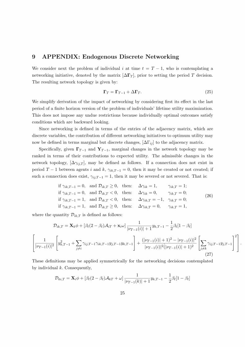
9 APPENDIX: Endogenous Discrete Networking

We consider next the problem of individual i at time t = T − 1, who is contemplating anetworking initiative, denoted by the matrix [∆ΓT ], prior to setting the period T decision.The resulting network topology is given by:

ΓT = ΓT−1 + ∆ΓT . (25)

We simplify derivation of the impact of networking by considering first its effect in the lastperiod of a finite horizon version of the problem of individuals’ lifetime utility maximization.This does not impose any undue restrictions because individually optimal outcomes satisfyconditions which are backward looking.

Since networking is defined in terms of the entries of the adjacency matrix, which arediscrete variables, the contribution of different networking initiatives to optimum utility maynow be defined in terms marginal but discrete changes, [∆Γij ] to the adjacency matrix.

Specifically, given ΓT−1 and YT−1, marginal changes in the network topology may beranked in terms of their contributions to expected utility. The admissible changes in thenetwork topology, [∆γij,T ], may be defined as follows. If a connection does not exist inperiod T − 1 between agents i and k, γik,T−1 = 0, then it may be created or not created; ifsuch a connection does exist, γij,T−1 = 1, then it may be severed or not severed. That is:

if γik,T−1 = 0, and Dik,T ≥ 0, then: ∆γik = 1, γik,T = 1;if γik,T−1 = 0, and Dik,T < 0, then: ∆γik = 0, γik,T = 0;if γik,T−1 = 1, and Dik,T < 0, then: ∆γik,T = −1, γik,T = 0;if γik,T−1 = 1, and Dik,T ≥ 0, then: ∆γik,T = 0, γik,T = 1,

(26)

where the quantity Dik,T is defined as follows:

Dik,T = Xkφ + [β`(2− β`)AiT + xiω]1

|νT−1(i)|+ 1yk,T−1 − 1

2β`[1− β`]

1|νT−1(i)|2

y2

k,T−1 +∑

j 6=i

γij,T−1γik,T−1yj,T−1yk,T−1

+

(|νT−1(i)|+ 1)2 − |νT−1(i)|2|νT−1(i)|2(|νT−1(i)|+ 1)2

∑

j 6=k

γij,T−1yj,T−1

2 .

(27)These definitions may be applied symmetrically for the networking decisions contemplatedby individual k. Consequently,

Dki,T = Xiφ + [β`(2− β`)AkT + ω]1

|νT−1(k)|+ 1yk,T−1 − 1

2β`[1− β`]

25

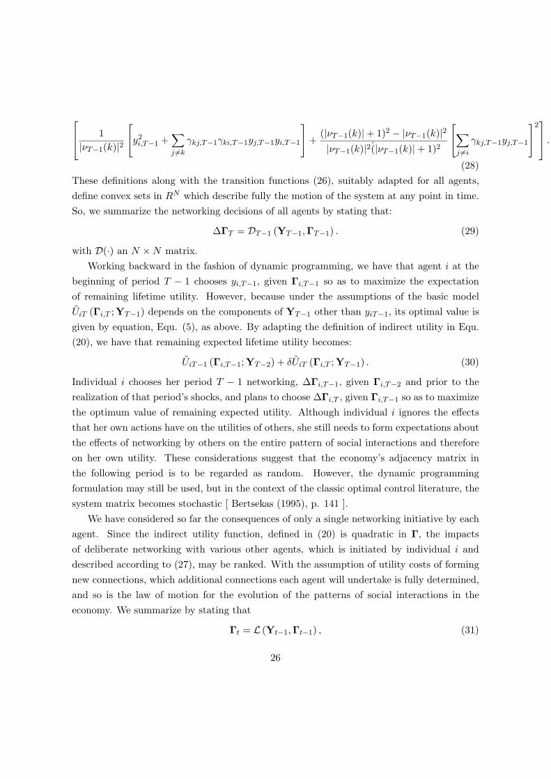
1|νT−1(k)|2

y2

i,T−1 +∑

j 6=k

γkj,T−1γki,T−1yj,T−1yi,T−1

+

(|νT−1(k)|+ 1)2 − |νT−1(k)|2|νT−1(k)|2(|νT−1(k)|+ 1)2

∑

j 6=i

γkj,T−1yj,T−1

2 .

(28)These definitions along with the transition functions (26), suitably adapted for all agents,define convex sets in RN which describe fully the motion of the system at any point in time.So, we summarize the networking decisions of all agents by stating that:

∆ΓT = DT−1 (YT−1,ΓT−1) . (29)

with D(·) an N ×N matrix.Working backward in the fashion of dynamic programming, we have that agent i at the

beginning of period T − 1 chooses yi,T−1, given Γi,T−1 so as to maximize the expectationof remaining lifetime utility. However, because under the assumptions of the basic modelUiT (Γi,T ;YT−1) depends on the components of YT−1 other than yiT−1, its optimal value isgiven by equation, Equ. (5), as above. By adapting the definition of indirect utility in Equ.(20), we have that remaining expected lifetime utility becomes:

UiT−1 (Γi,T−1;YT−2) + δUiT (Γi,T ;YT−1) . (30)

Individual i chooses her period T − 1 networking, ∆Γi,T−1, given Γi,T−2 and prior to therealization of that period’s shocks, and plans to choose ∆Γi,T , given Γi,T−1 so as to maximizethe optimum value of remaining expected utility. Although individual i ignores the effectsthat her own actions have on the utilities of others, she still needs to form expectations aboutthe effects of networking by others on the entire pattern of social interactions and thereforeon her own utility. These considerations suggest that the economy’s adjacency matrix inthe following period is to be regarded as random. However, the dynamic programmingformulation may still be used, but in the context of the classic optimal control literature, thesystem matrix becomes stochastic [ Bertsekas (1995), p. 141 ].

We have considered so far the consequences of only a single networking initiative by eachagent. Since the indirect utility function, defined in (20) is quadratic in Γ, the impactsof deliberate networking with various other agents, which is initiated by individual i anddescribed according to (27), may be ranked. With the assumption of utility costs of formingnew connections, which additional connections each agent will undertake is fully determined,and so is the law of motion for the evolution of the patterns of social interactions in theeconomy. We summarize by stating that

Γt = L (Yt−1,Γt−1) , (31)

26

where the function L(·) summarizes the above results.A number of remarks are in order. First, we note that although the law of motion (31)

is stated in terms of quantities that are known as of time t, the evolution of the state ofthe economy over time depends on realizations of shocks in every period. Second, althoughthe contribution to agent i’s utility from opening up a connection with agent k is definedsymmetrically to the contribution to agent k’s utility from opening up a connection withagent i, those two different contributions need not both have the same sign. This raisesthe possibility that opening and severing of connections would cycle, unless we impose thecondition that directly affected agents must be in mutual agreement. However, presence ofcosts does introduce friction, which mitigates some of these issues. Third, an extension of themodel would be to allow individual the option of initiating contacts with others according toa Poisson clock in the style of Blume (1993).

27