Social interactions in voting behavior: distinguishing between strategic voting and the bandwagon effect

Social interactions in voting behavior: distinguishing between strategic voting and the bandwagon effect

Haldun Evrenk Department of Economics, TOBB Economics and Technology University

Ankara, Turkey

Chien-Yuan Sher* Department of Business Management, National Sun Yat-Sen University

Kaohsiung, Taiwan

Abstract Prior studies of strategic voting in multi-party elections potentially overestimate the extent of it by counting erroneously votes cast under different motivations as strategic votes. We propose a method that corrects some of this overestimation by distinguishing between strategic voting (voting for a candidate other than the most preferred one to reduce the likelihood of an election victory by a third candidate that is disliked even more) and the votes cast under the ‘bandwagon effect’ (voting for the expected winner instead of the most preferred party to conform to the majority or to be on the winning side). Our method follows from the observation that a vote cannot be strategic unless the voter believes that it will affect the outcome of the election with a non-zero probability, while a vote cast under the bandwagon effect requires no such belief. Employing survey data that include the respondent’s assessment of the importance of his vote, we illustrate this method by estimating the extent of strategic voting in the 2005 UK general election. The estimated extent of strategic voting (4.22%) is strictly less than self-reported strategic voting (6.94%), but the discrepancy cannot be attributed in a statistically significant way to the bandwagon effect, suggesting that motivations other than those identified in the literature may be at work.

Keywords: voting behavior, social interactions, strategic voting, bandwagon effects, multi-party competition.

JEL classification: D71, D72, D84

* Author for correspondence; Tel: +886-7-5252000 ext. 4629; Email: [email protected]

mailto:[email protected]

1

Social interactions in voting behavior: distinguishing between strategic voting and the ‘bandwagon effect’

1. Introduction

In a multi-candidate election using a ‘first past the post’ rule, a voter may cast a vote for

candidate B even though his most preferred candidate is A. Such behavior is referred to as

strategic voting if all of the following conditions hold: (i) the voter thinks that the race will be

between parties B and C (and, possibly others, except A), (ii) the voter prefers B among those

listed in (i), and (iii) the voter believes that his vote will affect the outcome of the race with a

non-zero probability. Since the extent of strategic voting is crucial to the outcome of political

competition, several empirical studies estimate it. They all find that a non-trivial fraction of

the electorate votes for a party other than the most preferred one.1 Given the available data,

however, these studies cannot verify that all three conditions mentioned above hold for each

vote classified as strategic. Instead what they typically count is the number of misaligned

votes, i.e., votes cast for a lower ranked party or candidate (Kawai and Watanabe 2013).

A misaligned vote, however, may instead be explained by other motives, such as

preferences for conformity (or the wish to align oneself with the winner), known as the

‘bandwagon effect’. If this is the case, then earlier studies overestimate the extent of strategic

voting. In this paper we present a method for distinguishing between strategic voting and the

‘bandwagon effect’ or other social interaction effects with the appropriate data. Then, we

apply the method to the 2005 general elections in the United Kingdom.

The idea behind our method is as follows. Strategic voting follows from the

instrumentalist approach to voting (Downs 1957; Tullock 1967). Summarized by Downs

(1957, p. 7) as “The political function of elections in a democracy.... is to select a 1 In the UK general election of 1987, an estimated 6.3% to 17% of voters chose not to vote for their most preferred party, essentially because they did not believe that its candidate could win the election (Heath 1991; Niemi, Whitten and Franklin 1992). Similarly, in Canada it is estimated that 6% (3%) of voters in 1988 (1997) voted strategically (Blais and Nadeau 1996; Blais, Nadeau, Gidengil and Nevitte 2001).

2

government. Therefore rational behavior in connection with elections is behavior towards

this end and no other,” this approach implies that every vote (whether strategic or not) is the

result of a calculation of its effect on the outcome of the election. Under the ‘bandwagon

effect’, however, a vote is cast with no concern about that particular vote’s effect on the

outcome. Thus, a misaligned vote is a strategic vote only if the condition (iii) above holds,

i.e., the voter expects, however unrealistically, that his vote will be decisive.2 Otherwise, a

misaligned vote is cast owing to other factors, such as the ‘bandwagon effect’.

To illustrate our method, we employ data obtained from the 2005 British Election

Studies (BES) survey, identifying both the voters’ expectations about the UK’s 2005 general

election results their perspectives on the importance of their votes.3 In our sample, strategic

voting was self-reported by 6.94% of the respondents. Analyzing the interaction between

voting behavior, voter preferences and their stated expectations, we find that 4.22% of the

voters casting their ballots for the three main parties in England had voted strategically,

while 5.53% of the voters did not vote for their preferred party, because they chose to align

themselves with the expected winner or runner-up, or because they voted strategically. Even

though strategic voting does not explain all of the misaligned voting in the sample, the

‘bandwagon effect’ was not found to be statistically significant. Those who felt that their

ballots would have no impact on the election’s outcome tended to vote for the runner-up

rather than for the expected winner. This result calls (and, suggests ideas) for further

theoretical and empirical analysis of misaligned voting.

The remainder of this paper is organized as follows. In Section 2 the identification

methods used in earlier studies of strategic voting and their potential pitfalls are discussed.

In that section we also discuss the bandwagon effect in more detail. Section 3 presents a

2 As summarized in Table 3, most of the voters in our sample do expect that their vote will affect the outcome of the race. 3 This election took place on 5 May 2005 (a working day) electing members to the House of Commons based upon the ‘first past the post’ system. Three major parties, Labour, Conservatives and the Liberal Democrats, promoted candidates in almost every constituency, with the notable exception of Northern Ireland.

3

detailed discussion of the 2005 BES survey, with particular focus on how using the

respondents’ perspectives and expectations would help one to avoid the potential pitfalls

mentioned in Section 2. The empirical model utilized in this study is described in Section 4,

with Section 5 subsequently reporting the results. Finally, Section 6 concludes.

2. Literature review

2.1 Strategic voting: Two methods of identification

The empirical literature on strategic voting adopts both direct and indirect methods to

identify strategic voters (Blais, Young and Turcotte 2005). The former relies on the responses

provided by voters regarding their intentions when they vote, as the means of detecting

strategic voting. Many academically conducted national voter surveys, including the BES

survey employed in our work, regularly ask respondents to state the main reason for their

electoral choice. The (closed-end) options for this question include agreement with the

statement: “I really preferred another party but [the candidate] stood no chance of winning

in my constituency” or a statement using similar wording. Studies using the direct method

classify respondents who provide such answers as their main reason for voting as strategic

voters. Studies using the indirect method model the effect of both individual preferences and

strategic considerations on voting behavior, estimate these effects and generate predicted

vote shares with and without strategic considerations (see, for example, Alvarez and Nagler

2000, Blais et al. 2001 and Alvarez, Boehmke and Nagler 2006). The difference between

the two predictions supplies an estimate of the extent of strategic voting.

We mainly employ the indirect method herein, but our work differs from earlier studies

insofar as it includes the respondent’s perspective on the importance of his vote when

modeling voting behavior. If the respondent does not think that his vote will have any effect

on the probability of victory of the party for which he votes, then his misaligned vote cannot

4

be considered to be a strategic vote. The endogenous social effects literature discussed

below provides a possible alternative explanation, the ‘bandwagon effect’, for the

misaligned vote cast by such a voter.

2.2 The bandwagon effect

Manski (1993, p. 531) defines endogenous social effects as those “wherein the propensity of

an individual to behave in some way varies with the prevalence of that behavior in some

reference group containing the individual”. Endogenous social effects may have different

names in various contexts, such as ‘social interactions’, ‘peer-group influence’, ‘social

contagion’, or ‘bandwagon effect’.4 Unlike strategic voting, the bandwagon effect simply

follows from a desire to conform to the behavior of the voting majority and be on the side of

the winner (Nadeau, Cloutier and Guay 1993). Such a desire is commonly documented (see,

for example, Asch 1956).5

It is important to note that the difference between the bandwagon effect and strategic

voting does not lie in the degree of rationality these assumptions impose on the voter. An

early proponent of the modeling assumption that voters like to be on the winning side,

Hinich (1981, p. 135) argues that the assumption that voters tend to vote for the winner “is

no less plausible than the assumption that voters believe they can be pivotal”. According to

both Fey (1996) and Hodgson and Maloney (2012), conformity can be explained by a

rational motivation, with individuals tending to follow the majority essentially because they

believe that the majority is more informed than is any one individual.6

4 Considering the negative connotation of the term ‘endogeneity’ in empirical papers, we use the term social effects throughout the remainder of this paper. 5 Note that strategic voting, too, can be regarded as a special type of endogenous social effect: in a race with three candidates when most voters tend to vote for candidates B and C, if voter i votes for candidate B instead of his most preferred candidate A to reduce the probability that his least preferred candidate C wins the election, he is reacting to the behavior of other voters. 6 Callander (2007, p. 654), however, argues that within the context of the US presidential primary elections the desire to conform to the majority “is critical to the existence of voting bandwagons as they cannot be driven solely by an informational incentive to elect the better candidate.”

5

The discussion of the bandwagon effect dates back to the early twentieth century in the

United Kingdom, when polling was staggered over several days. Many commentators

believed that the bandwagon effect caused the winner on the first day to benefit in later

polling. Consequently, the Reform Act of 1918 required that all polling must occur on the

same day (Hodgson and Maloney 2012). In their experiments in the United States, Goidel

and Shields (1994) found that ‘independents’ tended to vote for a Republican candidate if he

was expected to win, and that ‘weak Republicans’ were likely to vote for a Democratic

candidate who was expected to win.

2.3 Potential overestimation of the extent of strategic voting

The main point of this paper is that by ignoring other types of social effects, prior empirical

studies of strategic voting may actually have incorporated various other social interactions

into their interpretations of the reasons underlying votes cast. More specifically, the

identification of strategic voters using the direct method may well have included voters

motivated by the bandwagon effect. Empirical studies using the indirect method may exhibit

the same flaw.

For example, when modeling actual voting behavior, Blais et al. (2001) constructed a

‘no chance’ variable to represent strategic considerations. That variable measured the

distance between the expected likelihood of victory for a particular party vis-à-vis the

expected winner (an example illustrating the construction of this variable is provided below).

They then regressed the respondents’ stated votes on party identification, the respondents’

ratings of each party, the respondents’ ratings of each party leader, and the ‘no chance’

variable. Assuming that those voters who shunned the candidates who had ‘no chance’ of

winning voted strategically, Blais et al. (2001) determined that in the 1997 Canadian

election, approximately 3% of the respondents were strategic voters. However, these voters

may well have been motivated by other factors, such as the bandwagon effect.

6

Another potential problem with such studies is the way in which voter expectations are

assessed. Regardless of whether voting is strategic or in conformance with the majority, the

voting decision is based upon the voter’s expectations about an election’s outcome, as

opposed to real voting behavior that is taking place at the polls. Several earlier studies

assume that voter expectations can be represented by the results of the previous elections

(adaptive expectations) or by the results of the current election (rational expectations

grounded in pre-election polls), but as we discuss in the next section, the voters’ responses

to survey questions do not justify either assumption.7

In addition, studies imposing either adoptive or rational expectations, typically

assume common knowledge, i.e., that every voter in the same constituency has the same

expectations.8 Yet, voter expectations are distinct from election results, and they typically

vary among different individuals. As Palfrey (1989, p. 69) suggests, if all voters have the

same perspective on the electoral situation in a society of rational voters, “multi-candidate

contests under the plurality rules should result in only two candidates getting any votes”.

These issues are dealt with in the present study by removing any of these assumptions

about voters’ expectations and behavior from the analysis. We instead employ survey data on

voters’ expectations of the election results and their perspectives on the importance of the

votes they cast in determining those results. Data on subjective expectations also provide

additional information, which enables one to distinguish between social interactions,

7 The concern is not just about the how well the assumption comports with reality. For instance, using the indirect method Alvarez and Nagler (2000) and Alvarez et al. (2006) estimate the extent of strategic voting. They assume that the results of the previous election are used as basis of strategic consideration, i.e., voters regard the party that had received the fewest votes in the previous election as the party that has no chance of victory in the current election. However, the party receiving the fewest number of votes in the previous election in a particular constituency may well decide to exert very little effort into that constituency in the current election; thus, the findings of the papers cited above may indicate nothing more than the fact that voters in a specific constituency were exposed to very little advertising relating to the weakest candidate; this clearly does not amount to social interaction. When this is the case, their findings actually indicate correlated effects, whereby individuals in a group tend to behave similarly because they are in similar environments (Manski 1993). 8 For recent theoretical studies that attempt to relax the common knowledge assumption, see Myatt (2007) and Clough (2007).

7

contextual effects and correlated effects (Manski 1993, 2004).9 In the next section, we

discuss our data in detail.

3. Measuring voters’ perspectives and expectations

3.1 The extent of misaligned voting

The primary data source for the present study is the dataset compiled from the survey

responses to the 2005 British Election Study (BES 2005). The overall study comprised a

series of linked surveys, two of which, the ‘BES pre-election cross-sectional survey’ and the

‘BES post-election panel and cross-sectional survey’, are particularly relevant to us.10

In 2005, the BES largely following the direct method referred to in Section 2, the

following question in the post-election survey is used to calculate the approximate number of

voters who did not vote for their preferred party essentially because they felt that their

first-ranked preference would not win:

“People give different reasons for why they vote for one party rather than another; which of the following best describes your reasons? (NCSR2005b, p.15)

1. The party had the best policies; 2. The party had the best leader; 3. I really preferred another party but [the candidate] stood no chance of

winning in my constituency; 4. I voted tactically (Volunteered); 5. Other (Write In).”

As discussed above, a response of either 3 or 4 is consistent with strategic considerations, the

bandwagon effect or other unexplored factors; we simply refer to such behavior as misaligned

voting. The survey data also tell us which party these voters really preferred, i.e., their

‘reported sincere voting.’ Comparing that party with the party they eventually voted for, we

9 Contextual effects are those in which the propensity of an individual to behave in a certain manner varies according to the exogenous characteristics of the group (Manski 1993). 10 The 2005 BES also provides a series of weighting factors to correct for the probability of unequal selection, fitting the sample profile to population estimates for Britain, England, Scotland or Wales.

8

find that not all of the voters reporting misaligned voting actually had cast a misaligned vote.

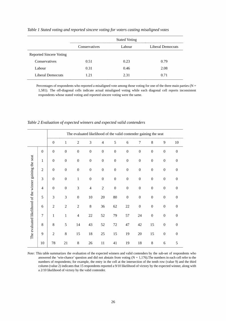
Table 1 shows the actual number of misaligned votes as well as their distribution.

<Table 1 is inserted about here>

In Table 1, the cells indicate the percentages of reported misaligned votes among those

respondents who cast ballots for one of the three main political parties. For example, the

entry in the second cell of the ‘Conservatives’ row indicates that 0.23% of those who had

cast their votes voted for the Labour Party, but they actually preferred the Conservatives.

Each diagonal cell reports the share of inconsistent responses, that is, voters for whom

reported votes and stated sincere preferences were identical, despite the respondent’s claim

that he or she had cast a misaligned vote. In our dataset, 1.68% of all of the voters who had

cast their ballots for one of the three main parties exhibited such ‘confusion’: they had

failed, over time, to provide consistent answers to the questionnaire.11 Information reported

in the off-diagonal cells in this table (the direct method) reveals that in England in 2005,

6.94% of the votes were misaligned.

3.2 Measuring voter expectations of election results

Answers to the following ‘win-chance’ question from the pre-election survey are used to

measure the expectations of voters regarding the upcoming election’s results:

On a scale that runs from 0 to 10, where 0 means very unlikely and 10 means very likely, how likely is it that Labour/Conservative Party/Liberal Democrats will win the election in this constituency? (NCSR2005a, p. 19)

With responses ranging from 0 to 10, this question can in principle be used to obtain a

subjective measure of the likelihood of each party winning in each respondent’s

constituency. There are, however, two issues that require careful consideration before

constructing such a measure. 11 Strategic voters should also believe that their vote is decisive. Respondents selecting either answer 3 or 4, however, are not, with any statistical significance, more likely to believe that that the votes they cast could affect the election results (p = 0.455). A possible reason for this result is that such respondents included not only strategic voters, but also voters who either were motivated by other factors or provided ‘confused’ responses.

9

First, as Blais, Gidengil, Fournier, Nevitte and Hicks (2008) note, survey the

respondents’ answers depend on the way in which a question on subjective voter

probabilities is framed. When respondents were asked whether each party had a chance of

winning, and then asked to rate their chances on a scale of 0 to 100,12 they tended to

respond negatively in the first instance (reported that many candidates had no chance of

winning), but they seemed reluctant to select 0 when asked directly asked to rate the overall

chance of winning on a 0 to 100 scale. Thus, candidates who were perceived to have no

chance of winning according to the initial question’s wording could be perceived as having

a positive (albeit small) chance of winning when using the alternative question’s wording.13

Second, as the same scale may have dissimilar meanings for different respondents, such

subjective evaluations might be incomparable across respondents. Consider, for example, the

scenario in which two Conservative supporters, voters T and K, assign the following ordinal

scores to (respectively) Labour’s, Liberal Democrats’ and Conservatives’ chances winning a

seat: T’s response is 5, 4 and 2, and K‘s response is 9, 6, and 5. To be able to compare these

two responses, Blais et al. (2001) proposes construction of a ‘no chance’ variable, which

equals the distance between a particular party’s expected chance of winning the election party

vis-à-vis the expected winner. For voter T, the value of the ‘no chance’ variable for the

Conservatives is 3 (= 5 – 2), while for voter K it is 4 (= 9 – 6). Thus, according to Blais et al.

(2001), voter K is more willing to give up on the Conservatives than voter T, essentially

because voter K is less confident of a Conservative victory. However, this contradicts the

original responses to the question, which clearly suggest that voter K was more optimistic of a

12 This was the question framing used in the 2004 Canadian Election Study. 13 The initial question’s wording invites a yes-no question, which may cause a problem. Manski (2004) noted that when asking respondents to give their subjective probabilities of certain events, a yes-no question easily overlooks essential information; for example, if respondents are asked whether they will vote on Election Day, a no answer does not mean that the probability of participation is zero. Manski (2004) stated that it should mean that the subjective probability of respondent turning out is small enough that a tentative ‘no’ answer is more accurate than a ‘yes’ one. Similarly, in the Blais et al. (2008) study, when respondents were asked whether a particular party had a chance of winning using the initial question’s wording, a ‘no’ answer did not indicate that the subjective probability of the event was zero, but rather that it was small.

10

Conservative victory than voter T.

Owing to these two issues, using the response to the ‘win-chance’ question directly

may be problematic. While the absolute values of voter responses appear to be unreliable in

the above scenario, the subjective chance ranking elicited by the question is the same for

both voters T and K: Labour > Liberal Democrats > Conservatives. For that reason, we use

the subjective chance ranking elicited from voter responses in most of this study.14 The

party perceived to have the highest probability of winning in the respondent’s constituency

in the pre-election survey is referred as the ‘winner’, and the party with the second highest

probability of winning is referred as the ‘valid contender’.

The evaluations of the expected winner and the valid contender by those voters within

the sub-set of respondents who answered the ‘win-chance’ question and did not abstain from

voting (N = 1,176) are summarized in Table 2. Each cell refers to the number of respondents

who provided two specific evaluations on the likelihood of victory by the expected winner

and the valid contender; for example, the entry in the cell at the intersection of the tenth row

(value 9) and the third column (value 2) indicates that 15 respondents reported a 9/10

likelihood of victory by the expected winner, along with a 2/10 likelihood of victory by the

valid contender.15


BES 2005 pre-election survey data shows that voters’ predictions in the England sample

(N = 1,929) are highly inaccurate. Within various constituencies, 856 (44.38%) of the

respondents predicted the wrong winner, while 984 (51.01%) predicted the wrong runner-up.

14 We employ the ‘no chance’ variable developed by Blais et. al. (2001) only in one of the extensions, where we need to identify strong and weak runner-ups (see footnote 24). 15 A few special cases with two or more candidates receiving the same win chance are handled as follows. If a voter did not predict the winner, but believed that each of the three candidates were equally likely to win (or, two were equally likely to win and one less likely to win), then for this voter we do not have a predicted winner but just three (or two) valid contenders. If a respondent assigned a high value to one candidate and a lower (but identical) value to the two other candidates; we say that he or she predicted a winner and two valid contenders. If a respondent assigned a high chance to one candidate and a zero chance to the other two, we say that he or she predicted only a winner and no valid contenders.

11

In a close competition, this could be expected, i.e., actual winner could conceivably have been

regarded as the valid contender and the runner-up as the expected winner. In this specific case,

however, 966 (50.08%) selected a candidate in the top two who did not attain either

position.16 Survey data does not confirm the uniform expectations assumption either: voters

within the same constituencies were found to have quite differing perspectives on the

election results. In Aldridge-Brownhills constituency, for example, 21 respondents answered

the ‘win-chance’ question, 16 predicted a Conservative victory, while 5 predicted a Labour

victory. Conservative candidate won 47.4% of the vote and the election while Labour

candidate got 33.5% of the vote. In other constituencies, the predictions of the winner

provided by respondents within the same constituencies were similarly diverse.17

Past election results do a particularly bad job in predicting current voter expectations.

In the England sample (N = 1,929) of the BES pre-election survey administered prior to the

2005 general election, 802 (41.58%) of the respondents believed that the winner of the

election in their constituency would not be the same party that had won in the 2001 election,

934 (48.42%) believed that the valid contender in the 2005 election would not be from the

same party that placed second in the 2001 election, and 950 (49.25%) believed that the top

two parties in their constituencies would differ from those in the previous election.

3.3 Measuring the effects of voter expectations on their votes

To understand the motivations behind a misaligned vote, we also need to know the voter’s

assessment of the impact of his or her vote on the election’s outcome. The answer to the

following question from the BES 2005 pre-election survey is used to infer voters’

expectations about the salience of their votes:

On a scale from 0 to 10, where 0 means very unlikely and 10 means very likely, how

16 In other words, 966 of the respondents had incorrect expectations for who would be the top twon candidates in their constituencies. 17 These results confirm several studies arguing that a substantial proportion of the public is uninformed about politics, e.g.,, Zaller (1992), Converse (2000), Friedman (2006) and Adams, Ezrow and Somer-Topcu (2011).

12

likely is it that your vote will make a difference in terms of which party wins the election in this constituency? (NCSR2005a, p. 58)

The frequency distribution of the subset of respondents who responded to this question and

did not abstain from voting is shown in Table 3 (N = 1,226).


It is worth noting that like their predictions about the winner of the election, voters’

assessments of the impact of their votes are quite unrealistic. Only a small set of

respondents believed that the effect of their vote would be trivial, i.e., provided a response

of 0.18

4. The model

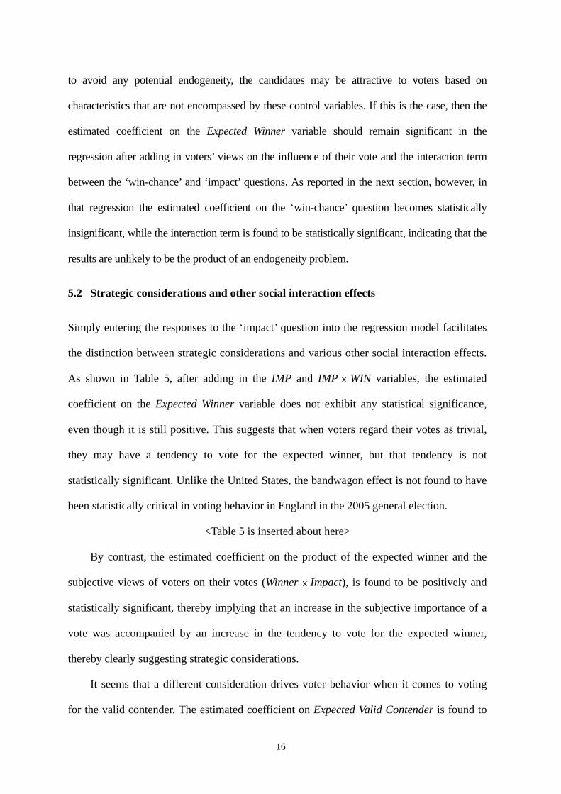
Standing in front of a voting booth, the utility voter j obtains from voting for party L is

assumed to be equal to

where XjL is a vector of the characteristics of party L relative to voter j; Dj is a vector of the

characteristics of the voters; εjL is the error term in the choice of voting for party L; and the

subjective response from the ‘win-chance’ question, WINjL, is a 2 x 1 index vector. If voter j

expects party L to win, then WINjL′ will be equal to [1,0]; if voter j expects party L to be a

valid contender, then WINjL′ will be equal to [0,1]. IMPj refers to the responses to the ‘impact’

question, indicating voter j’s perspective on how crucial he believes his vote to be.

The control variables used in this model comprise ‘party campaigning activities’,

‘candidate characteristics’ and ‘voter party identifications’, along with other standard

demographic variables. The control variables relevant to party campaigning activities reflect

parties’ expectations about the results, some (but not all, as we have noted above the voters

18 Unrealistic, but not totally irrational: a brief regression, not reported here, finds that a respondent’s answer to the ‘impact’ question was positively and significantly related to the inverse of the difference between the voting shares garnered by the top two parties in the respondent’s constituency, suggesting that as elections become more competitive, voters regard their votes as more crucial.

13

have diverse expectations on the outcome of the elections) voters may share those

expectations. Any major party that believes it has no chance of winning a constituency is

unlikely to exert much campaign effort into that constituency. Thus, if no variables controlling

the strength of the campaigning activities are included into the regression, then what is

estimated as the social interaction effect may instead be just the effect of the political

campaigning on voting behavior.

The 2005 BES post-election survey provides information on whether respondents were

contacted by a party agent or candidate in the form of four types of electioneering activities,

encompassing ‘doorstep canvassing’, ‘telephone canvassing’, ‘getting out the vote’ and

‘party election broadcasts’.19 Additional information also was collected in the pre-election

survey relating to party activities taking place prior to the campaign season, such as whether

the respondents were contacted by local party branches or whether the respondents had been

assisted by a party’s local MP.

Variables relevant to the characteristics of the candidate are: (i) an index of whether the

candidate in the respondent’s constituency is an incumbent; and (ii) an index of whether the

candidate in the respondent’s constituency is a ‘freshman’ candidate running for the same

party that won the last election (we refer to such a candidate as a ‘successor’ throughout the

paper). Thus, a candidate either is an ‘incumbent’, a ‘successor’ or a ‘challenger’.

An incumbent is the focal point within the constituency, and only on very rare

occasions will the incumbent be expected to receive the fewest votes in a three-party

election. By contrast, challengers must persuade voters that they are the valid contender;

otherwise they will be perceived as trailing in the election. In elections without an 19 ‘Doorstep canvassing’ involves a campaign team engaging in face-to-face interaction with voters, while ‘telephone canvassing’ involves personal interactions carried out over the telephone. The primary aim of canvassing is to disseminate relevant information on the candidate or the party, while also attempting to determine whether electors are party supporters. Based on this information, a campaign team sends people to contact those identified supporters on polling day to remind them to vote, referred to as ‘getting out the vote’ (GOTV). Since the inclusion of the GOTV variable may cause an endogeneity problem, it is excluded from our regression; however, our estimated doorstep and telephone canvassing effects also include the indirect effects of GOTV.

14

incumbent, e.g., when the incumbent chooses to retire, the successor becomes the focal

point. A preliminary regression suggests that voters were reluctant to believe that candidates

who were either incumbents or successors would be likely to obtain the fewest votes.

Control variables for the characteristics of each respondent include voter party

identifications and variables measuring the subjective distance between the respondent and

each party with regard to political issues (such as Britain’s membership in the European

Union, taxation, healthcare) as well as on an abstract one dimensional (left-right) policy space.

Those respondents who believed that their position on an issue was similar to that of a

particular party were allocated a smaller number in the political issue variables. Finally,

standard demographic variables, including age, gender, income, unemployment, house

ownership, union membership and whether the respondent worked in the public sector, are

also added into our proposed model.

We focus on elections in which only three main parties, Labour, Conservatives or

Liberal Democrats, effectively compete. As a result, our analysis is restricted to the sample

from England; other major parties, such as the Scottish National Party (SNP) and Plaid

Cymru, which invariably receive a moderate share of votes, field candidates in Scotland and

Wales.20 In some of the constituencies in England, other smaller parties (such as the Green

Party) exist, but collectively they garner only a slim vote share.21 We assume that the

existence of smaller, alternative parties does not alter the decisions of voters on the three

main parties.

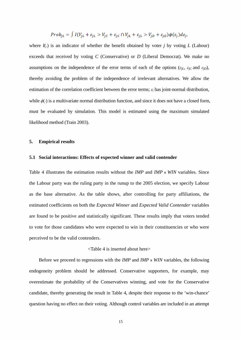
The model is estimated using multinomial probit, as opposed to multinomial logit. The

probability of voter j choosing party L is:

20 These strongly nationalist parties fielded no candidates in England. The provision of the option of two additional parties may have affected the decisions of voters with regard to the three main parties, while neglecting the choice of SNP or Plaid Cymru within the model would have created a problem in the Scotland and Wales samples; hence our focus only on the England sample. 21 The three constituencies in England where smaller parties or independent candidates won a seat were Bethnal Green and Bow, Blaenau Gwent and Wyre Forest.

15

,

where I(.) is an indicator of whether the benefit obtained by voter j by voting L (Labour)

exceeds that received by voting C (Conservative) or D (Liberal Democrat). We make no

assumptions on the independence of the error terms of each of the options (εjL, εjC and εjD),

thereby avoiding the problem of the independence of irrelevant alternatives. We allow the

estimation of the correlation coefficient between the error terms; εj has joint-normal distribution,

while ϕ(.) is a multivariate normal distribution function, and since it does not have a closed form,

must be evaluated by simulation. This model is estimated using the maximum simulated

likelihood method (Train 2003).

5. Empirical results

5.1 Social interactions: Effects of expected winner and valid contender

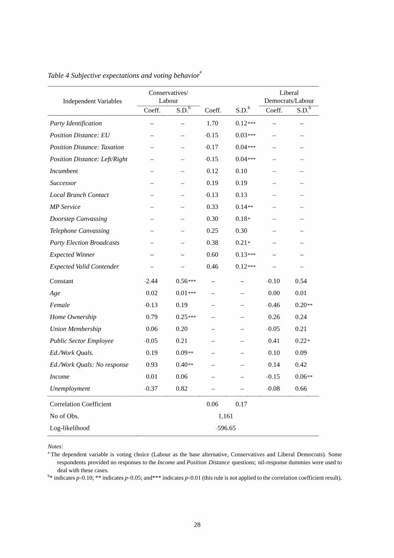
Table 4 illustrates the estimation results without the IMP and IMP x WIN variables. Since

the Labour party was the ruling party in the runup to the 2005 election, we specify Labour

as the base alternative. As the table shows, after controlling for party affiliations, the

estimated coefficients on both the Expected Winner and Expected Valid Contender variables

are found to be positive and statistically significant. These results imply that voters tended

to vote for those candidates who were expected to win in their constituencies or who were

perceived to be the valid contenders.


Before we proceed to regressions with the IMP and IMP x WIN variables, the following

endogeneity problem should be addressed. Conservative supporters, for example, may

overestimate the probability of the Conservatives winning, and vote for the Conservative

candidate, thereby generating the result in Table 4, despite their response to the ‘win-chance’

question having no effect on their voting. Although control variables are included in an attempt

16

to avoid any potential endogeneity, the candidates may be attractive to voters based on

characteristics that are not encompassed by these control variables. If this is the case, then the

estimated coefficient on the Expected Winner variable should remain significant in the

regression after adding in voters’ views on the influence of their vote and the interaction term

between the ‘win-chance’ and ‘impact’ questions. As reported in the next section, however, in

that regression the estimated coefficient on the ‘win-chance’ question becomes statistically

insignificant, while the interaction term is found to be statistically significant, indicating that the

results are unlikely to be the product of an endogeneity problem.

5.2 Strategic considerations and other social interaction effects

Simply entering the responses to the ‘impact’ question into the regression model facilitates

the distinction between strategic considerations and various other social interaction effects.

As shown in Table 5, after adding in the IMP and IMP x WIN variables, the estimated

coefficient on the Expected Winner variable does not exhibit any statistical significance,

even though it is still positive. This suggests that when voters regard their votes as trivial,

they may have a tendency to vote for the expected winner, but that tendency is not

statistically significant. Unlike the United States, the bandwagon effect is not found to have

been statistically critical in voting behavior in England in the 2005 general election.


By contrast, the estimated coefficient on the product of the expected winner and the

subjective views of voters on their votes (Winner x Impact), is found to be positively and

statistically significant, thereby implying that an increase in the subjective importance of a

vote was accompanied by an increase in the tendency to vote for the expected winner,

thereby clearly suggesting strategic considerations.

It seems that a different consideration drives voter behavior when it comes to voting

for the valid contender. The estimated coefficient on Expected Valid Contender is found to

17

be positively significant in Table 5, while the estimated coefficient on Valid Contender x

Impact is found to be insignificant.22 That is, there was a tendency among voters to vote for

the expected valid contender, regardless of how pivotal they though their votes would be.

So, this tendency is not motivated by voters’ expectations about their votes’ effects on

which party wins the election in their constituency. Since these voters tend to vote for the

expected contender instead of the expected winner, their behavior cannot be driven by the

desire to be on the winning side.

This support for valid contenders may indicate a social interaction effect that has not

been identified yet. Two possible explanations from the literature come to mind. First, by

voting for valid contenders, voters may be attempting to force the winning candidate to

moderate his policy, assuming that candidates do so in response to declines in their margins

of victory (see Razin 2003; Castanheira 2003).23 Second, the media, with its emphasis on

the importance of voting for the valid contender, could play a role (see de Vreese,

Boomgaarden and Semetko 2011; Jger 2012). Yet, our preliminary analysis indicates the

need for further empirical and theoretical studies to understand the determinants of the

support for valid contenders.24

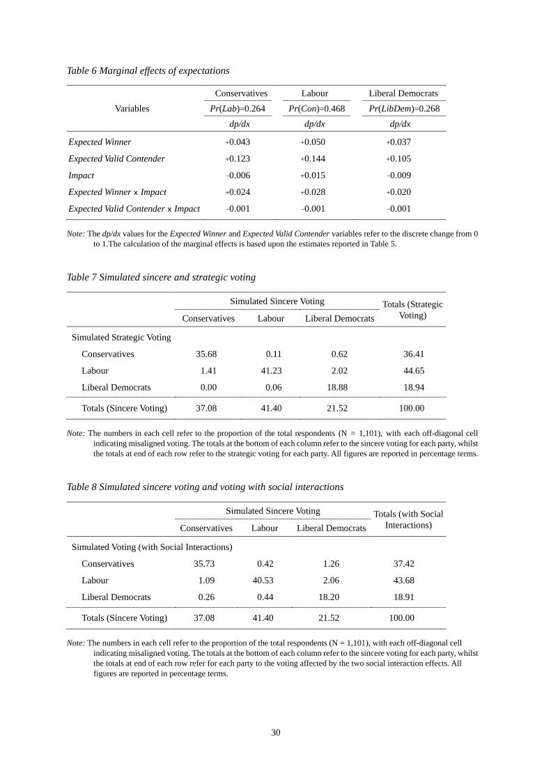
Next we study the marginal effects. For voter j, a marginal effect is a simulated change

in the probability of choosing party L if voter j believes that L either will win or be the valid

22 As explained in Section 3.2, when respondents believe that two or more candidates have the same likelihood of winning constituency seats, we classify all of them as valid contenders, not expected winners. Reclassifying those candidates as expected winners has no effect on the results. 23 The Castnaheira (2003) argument is, however, based on a two-party election, with no theoretical studies having yet applied their model to a three-party election. 24 We did some further analysis, categorizing valid contenders as ‘strong’ or ‘weak’, defining a valid contender as strong if the voters expect him to have a slightly smaller chance of victory than that of the winner; other valid contenders are then defined as weak. (Despite our assertion in Section 3.2, that the absolute values of the voters’ responses to the ‘win-chance’ question were incomparable, this work may, nevertheless, provide a rough idea of the types of valid contenders capable of attracting votes.) In the regression, the coefficient on the product of the strong valid contender and voters’ subjective assessments about on the influence of their votes is statistically significant, suggesting strategic considerations. The results also show that the estimated coefficient on the strong valid contender is statistically insignificant, while the estimated coefficient on the weak valid contender is positive and statistically significant. This implies, ceteris paribus, a tendency among voters to cast their ballots for weak valid contenders; none of the explanations mentioned above sheds much light on that finding.

18

contender within the constituency. We simulate several changes in choice probabilities,

altering both the perspectives of the respondents about the importance of their votes and the

interaction terms. The marginal effects, based upon the estimation results reported in Table

5, are reported in Table 6.


Let us assume that the original probability of voter j voting for the Conservatives is

0.264 if the party is neither the expected winner nor the valid contender. We can further

assume that voter j believes that his vote will have a 0/10 effect on the result. If voter j

believes that the Conservatives will win the constituency, the probability of voting

Conservative will increase to 0.307; this increment is the simulated effect of the incentive to

be on the winning side. Conversely, if voter j believes that his vote will have a 5/10 effect on

the result, the probability of voting Conservative increases to 0.397 [= 0.307 – 5(0.006) +

5(0.024)], with this 0.09 increment representing the simulated effect of strategic

considerations. Similarly, if voter j believes that the Conservative candidate is the valid

contender in the constituency, the probability of voting Conservative would increase to

0.387 when the effect is 0/10. If the influence were to be 5/10, the probability of voting

Conservative would be reduced to 0.352.

5.3 Misaligned votes attributable to social interactions

In order to compare the results of the present study with those of Alvarez and Nagler (2000)

and Alvarez et al. (2006), we use their methods to carry out a thought experiment. More

specifically, we use the estimation results from Table 5 to simulate voting without social

interactions (predicted sincere voting), then voting including only strategic considerations,

and then voting including all social interactions.

In order to simulate the sincere vote of each voter, the coefficients on WINjL, IMPj and

IMPj x WINj are all set at zero, and the utility from each candidate for each voter is

19

calculated using the other estimated coefficients. The candidate with the highest utility is

designated as the voter’s sincere choice. Similarly, in order to simulate the votes cast with

strategic considerations but without any other social interaction effect, we calculate the

simulated choice for each voter, this time setting only the coefficient of WINjL equal to zero.

Finally, we use the full model including all social interaction effects to calculate the

predicted voting.

If the simulated sincere voting by a voter differs from their voting with the inclusion of

only strategic considerations, then this finding is defined as strategic voting. If the simulated

sincere voting by a voter differs from their voting obtained from the full model, then we

define this as misaligned voting attributable to all social interactions. The simulated results

on sincere voting and voting with the inclusion of only strategic considerations are reported

in Table 7.


The entries along the main diagonal of the table represent the proportion of respondents

whose sincere votes and strategic votes were the same. Each of the off-diagonal cells shows

the proportion of respondents who voted strategically. For example, the entry in the second

row of the ‘Simulated Sincere Voting: Conservatives’ column indicates that 1.41% of the

respondents had a preference for the Conservatives, but voted for Labour for strategic

considerations. Of all the voters in the England sample casting their ballots for one of the

three main parties, 4.22% are found to have voted strategically.

The simulated results of sincere voting and voting affected by all of the social

interaction effects are reported in Table 8, wherein 5.53% of the voters in the England

sample are found to have misaligned their votes based upon social interaction effects. The

voting simulation based on the full model is found to correctly predict 78.64% of the

reported votes in the sample (N = 1,147).


20

Alvarez and Nagler (2000) estimated that of all the votes cast for the three main parties

in the 1987 UK general election, 7.2% were strategic votes; Evans and Heath (1993) also

estimated that 6.3% of the electorate voted strategically using the direct method (discussed

previously). Applying the direct method to the England sample, we find that, in the 2005

UK general election, 6.94% of the votes were misaligned. Yet, we also find that only 4.22%

of the voters in that election voted strategically; the discrepancy can be attributed to the

bandwagon effect or other factors.

6. Conclusion

In this study, we present a method that distinguishes between strategic voting, the

bandwagon effect and possibly other social interaction effects. Using survey data on voter

expectations and perspectives, we find that in the 2005 general election, voters in England

had a tendency to align themselves with the winning side, but this tendency was not found

to be statistically significant. By contrast, strategic considerations were a statistically

significant factor, but they do not explain all of what we call misaligned voting.

Furthermore, ceteris paribus, voters seem to have been significantly more inclined to vote

for valid contenders.

In the standard Downsian model with three candidates, a pure strategy Nash

equilibrium does not exist. Studies restoring the existence of equilibrium, e.g., Evrenk

(2009), and Evrenk and Kha (2011), introduce other factors such as valence into the model,

but leave intact the assumption that all votes are sincere. Identifying the extent of strategic

voting as well as other sources of misaligned voting in actual elections provides ideas on

how to improve theoretical models of spatial competition and their predictions as well. We

also hope that our findings on voter expectations and voter behavior will contribute to the

analysis of turnout in multi-party elections.

21

Appendix: Comparing alternative regressions

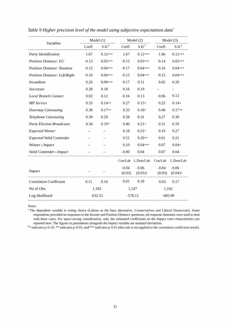
In this section we run our main regression under the assumptions adopted by earlier studies, i.e., that past or current election results can be used as a proxy for individual subjective expectations and that voter expectations are uniform in a district. Then, we compare our results with the results under these assumptions. As discussed in Section 2.3, some authors also assume that voters have rational expectations, i.e., they know the result of the election beforehand. Since regressing individual voting behavior on current election results (current group behavior) may give rise to endogeneity problems, we do not carry out such regressions in this comparison.25

When voters form their expectations based solely on the results of previous election and every voter in the same constituency has the same expectation, WINjL in the model is replaced by a vector of indices signifying whether a party candidate obtained the largest or second largest number of votes in the 2001 election in the constituency of voter j. The respondent’s answer to the ‘impact’ question, IMPj, still measures how crucial the ballot was, from the perspective of voter j.

Model (1) in Table 9 does not include the WIN, IMP or IMP x WIN variables, while Model (2) reports the results of the model based upon subjective expectations data (the partial results from Table 5). For comparative purposes, we also carry out a regression containing no variables of relevance to social interactions.


Model (3) shows that among all of the estimated coefficients on social interactions, only the one on the Winner x Impact variable is found to have any statistical significance. A comparison of Models (2) and (3) suggests that the estimated coefficients in Model (2), obtained using subjective expectations data, are more precise than those shown in Model (3).

The comparison of Models (1) and (2) indicates that after accounting for voter expectations, the estimated coefficients on the incumbent and successor variables were smaller, implying that the estimated coefficients on incumbents and successors spuriously capture the voter expectation’s effect when those variables are omitted. Indeed the coefficients in Model (1) capture two effects: the direct effect, a voter casts a vote for a candidate simply because he is the incumbent or the successor, and an indirect effect, a voter casts a vote for the

25 Although Brock and Durlauf (2003) show that under certain conditions, imposing current behavioral results on groups in a multinomial choice model does not produce an identification problem, the conditions (such as assuming that the error term, εjL, is independently and identically distributed across choices) are too strong for this study.

22

incumbent or the successor because he believes that the candidate is likely to win, or at least be a valid contender.

Acknowledgments

This paper is a heavily revised version of a chapter in the author’s PhD dissertation (Sher 2012). It has benefited greatly from the advice provided by Marc Rysman, Laurent Bouton and Daniele Paserman. Sincere gratitude is also extended to William F. Shughart, II, J. and Aki Lehtinen for many helpful comments. The usual disclaimer applies.

References

Adams, J., Ezrow, L., and Somer-Topcu Z. (2011). Is anybody listening? Evidence that voters do not respond to European parties’ policy statements during elections. American Journal of Political Science, 55(2), 370–382.

Alvarez, R. M. and Nagler, J. (2000). A new approach for modelling strategic voting in multiparty elections. British Journal of Political Science,30(1), 57-75.

Alvarez, R. M., Boehmke, F. J., and Nagler, J. (2006). Strategic voting in British elections. Electoral Studies, 25(1), 1-19.

Asch, S. E.(1956). Studies of independence and conformity: a minority of one against a unanimous majority. Psychological Monographs: General and Applied, 70(9), 1-70.

Blais, A., and Nadeau, R. (1996). Measuring strategic voting: a two-step procedure. Electoral Studies, 15(1), 39–52.

Blais, A., Nadeau, R., Gidengil, E., and Nevitte, N. (2001). Measuring strategic voting in multiparty plurality elections. Electoral Studies, 20(3), 343–352.

Blais, A., Young, R., and Turcotte, M. (2005). Direct or indirect? Assessing two approaches to the measurement of strategic voting. Electoral Studies, 24(2), 163–176.

Blais, A., Gidengil, E., Fournier, P., Nevitte, N., and Hicks, B. M. (2008). Measuring expectations: comparing alternative approaches. Electoral Studies, 27(2), 337-343.

Brock, W. and Durlauf, S. (2003). Multinomial choice with social interactions. Working paper, University of Wisconsin at Madison.

23

Callander, S. (2007). Bandwagons and momentum in sequential voting. Review of Economic Studies, 74(3), 653-684.

Castanheira, M. (2003). Victory margins and the paradox of voting. European Journal of Political Economy, 19(4), 817-841.

Clough, E. (2007). Strategic voting under conditions of uncertainty: a re-evaluation of Duverger's law. British Journal of Political Science, 37(2), 313-332.

Converse, P. E. (2000). Assessing the capacity of mass electorates. Annual Review of Political Science, 3, 331-353.

deVreese, C. H., Boomgaarden, H. G., and Semetko, H. A. (2011). (In)direct framing effects: the effects of news media framing on public support for Turkish membership in the European Union. Communication Research, 38(2), 179–205.

Downs, A. (1957) An economic theory of democracy. New York: Harper & Row

Evans, G., and Heath, A. (1993). A tactical error in the analysis of tactical voting: a response to Niemi, Whitten and Franklin. British Journal of Political Science, 23(1), 131-137.

Evrenk, H. (2009) Three-candidate competition when candidates have valence: the base case. Social Choice and Welfare, 32(1), 157-168.

Evrenk, H., and Kha, D. (2011) Three-candidate spatial competition when candidates have valence: stochastic voting. Public Choice, 147(3), 421-438

Fey, M. (1996). Informational cascades, sequential elections and presidential primaries. Paper presented at the annual meeting of the American Political Science Association, San Francisco, CA.

Friedman, J. (2006). Democratic competence in normative and positive theory: neglected implications of “the nature of belief systems in mass publics”. Critical Review: A Journal of Politics and Society, 18(1-3), 1-43.

Goidel, R. K., and Shields, T. G. (1994). The vanishing marginals, the bandwagon, and the mass media. Journal of Politics, 56(3), 802-810.

Heath, A. F. (1991). Understanding political change: the British voter 1964–1987. Oxford, UK: Pergamon Press.

24

Hinich, M. J. (1981). Voting as an act of contribution. Public Choice, 36(1), 135-140.

Hodgson, R., and Maloney, J. (2012). Bandwagon effects in British elections, 1885-1910. Public Choice, 157(1-2), 73-90.

Jger, K. (2012). Why did Thailand's middle class turn against a democratically elected government? The information-gap hypothesis. Democratization,19(6), 1138-1165.

Kawai, K., and Watanabe, Y. (2013). Inferring strategic voting. American Economic Review, 103(2): 624-662.

Manski, C. F. (1993). Identification of endogenous social effects: the reflection problem. Review of Economic Studies, 60(3), 531-542.

Manski, C. F. (2004). Measuring expectations. Econometrica, 72(5), 1329-1376.

Myatt, D. P. (2007). On the theory of strategic voting. Review of Economic Studies, 74(1), 255-281.

Nadeau, R., Cloutier, E., and Guay, J.-H.(1993). New evidence about the existence of a bandwagon effect in the opinion formation process. International Political Science Review, 14(2), 203-213.

NCSR (2005a) British Election Study 2005 pre-election wave: draft documentation of the Blaise questionnaire. London, UK: National Centre for Social Research.

NCSR (2005b) British Election Study 2005 post-election wave: draft documentation of the Blaise questionnaire. London, UK: National Centre for Social Research.

Niemi, R., Whitten, G. and Franklin, M. (1992).Constituency characteristics, individual characteristics and tactical voting in the 1987 British general election. British Journal of Political Science, 22(2), 229–240.

Palfrey, T. (1989).A mathematical proof of Duverger’s law. In Peter C. Ordeshook (ed.), Models of strategic choice in politics. Ann Arbor, MI: University of Michigan Press, pp.69-92.

Razin, R. (2003). Signaling and election motivations in a voting model with common values and responsive candidates. Econometrica, 71(4), 1083–1119.

Sher, C-Y. (2012). Voting Behavior and Political Campaigns. PhD Dissertation submitted to

25

Graduate School of Arts and Sciences, Boston University. Boston, MA

Train, K. (2003). Discrete choice methods with simulation. New York, NY: Cambridge University Press.

Tullock, G. (1967) Toward a mathematics of politics. Ann Arbor: University of Michigan Press.

Zaller, J. (1992). The nature and origins of mass opinion. Cambridge, UK: Cambridge University Press.

26

Table 1 Stated voting and reported sincere voting for voters casting misaligned votes

Stated Voting

Conservatives Labour Liberal Democrats

Reported Sincere Voting

Conservatives 0.51 0.23 0.79 Labour 0.31 0.46 2.08 Liberal Democrats 1.21 2.31 0.71

Percentages of respondents who reported a misaligned vote among those voting for one of the three main parties (N =

1,581). The off-diagonal cells indicate actual misaligned voting while each diagonal cell reports inconsistent respondents whose stated voting and reported sincere voting were the same.

Table 2 Evaluation of expected winners and expected valid contenders

The evaluated likelihood of the valid contender gaining the seat

0 1 2 3 4 5 6 7 8 9 10

The

eval

uate

d lik

elih

ood

of th

e w

inne

r gai

ning

the

seat

0 0 0 0 0 0 0 0 0 0 0 0

1 0 0 0 0 0 0 0 0 0 0 0

2 0 0 0 0 0 0 0 0 0 0 0

3 0 0 1 0 0 0 0 0 0 0 0

4 0 0 3 4 2 0 0 0 0 0 0

5 3 3 0 10 20 80 0 0 0 0 0

6 2 2 2 8 36 62 22 0 0 0 0

7 1 1 4 22 52 79 57 24 0 0 0

8 8 5 14 43 52 72 47 42 15 0 0

9 2 8 15 18 25 15 19 20 15 0 0

10 78 21 8 26 11 41 19 18 8 6 5 Note: This table summarizes the evaluation of the expected winners and valid contenders by the sub-set of respondents who

answered the ‘win-chance’ question and did not abstain from voting (N = 1,176).The numbers in each cell refer to the numbers of respondents; for example, the entry in the cell at the intersection of the tenth row (value 9) and the third column (value 2) indicates that 15 respondents reported a 9/10 likelihood of victory by the expected winner, along with a 2/10 likelihood of victory by the valid contender.

27

Table 3 Perceptions among voters of the impact of their votes

Evaluated Impact of Votes No. of Respondents

0 (trivial) 174 1 77 2 123 3 128 4 72 5 159 6 94 7 127 8 120 9 48

10 (important) 104 Note: This table reports the evaluated likelihood of the votes of the respondents ‘making a difference’, in terms of which

party would gain the seat in a constituency. The results show the frequency distribution of the responses to the ‘impact’ question by the sub-set of respondents who responded to this question and did not abstain from voting (N = 1,226).

28

Table 4 Subjective expectations and voting behaviora

Independent Variables Conservatives/

Labour Liberal Democrats/Labour

Coeff. S.D.b Coeff. S.D.b Coeff. S.D.b

Party Identification – – 1.70 0.12 *** – –

Position Distance: EU – – –0.15 0.03 *** – –

Position Distance: Taxation – – –0.17 0.04 *** – –

Position Distance: Left/Right – – –0.15 0.04 *** – –

Incumbent – – 0.12 0.10 – –

Successor – – 0.19 0.19 – –

Local Branch Contact – – –0.13 0.13 – –

MP Service – – 0.33 0.14 ** – –

Doorstep Canvassing – – 0.30 0.18 * – –

Telephone Canvassing – – 0.25 0.30 – –

Party Election Broadcasts – – 0.38 0.21 * – –

Expected Winner – – 0.60 0.13 *** – –

Expected Valid Contender – – 0.46 0.12 *** – –

Constant –2.44 0.56 *** – – –0.10 0.54

Age 0.02 0.01 *** – – 0.00 0.01

Female –0.13 0.19 – – –0.46 0.20 **

Home Ownership 0.79 0.25 *** – – 0.26 0.24

Union Membership 0.06 0.20 – – –0.05 0.21

Public Sector Employee –0.05 0.21 – – 0.41 0.22 *

Ed./Work Quals. 0.19 0.09 ** – – 0.10 0.09

Ed./Work Quals: No response 0.93 0.40 ** – – 0.14 0.42

Income 0.01 0.06 – – –0.15 0.06 **

Unemployment –0.37 0.82 – – –0.08 0.66

Correlation Coefficient 0.06 0.17

No of Obs. 1,161

Log-likelihood –596.65 Notes: a The dependent variable is voting choice (Labour as the base alternative, Conservatives and Liberal Democrats). Some

respondents provided no responses to the Income and Position Distance questions; nil-response dummies were used to deal with these cases.

b* indicates p<0.10; ** indicates p<0.05; and*** indicates p<0.01 (this rule is not applied to the correlation coefficient result).

29

Table 5 Subjective expectations, voting impact and voting behaviora

Independent Variables Conservatives/

Labour Liberal Democrats/Labour


Party Identification – – 1.67 0.12 *** – –

Position Distance: EU – – –0.15 0.03 *** – –

Position Distance: Taxation – – –0.17 0.04 *** – –

Position Distance: Left/Right – – –0.15 0.04 *** – –

Incumbent – – 0.17 0.11 – –

Successor – – 0.16 0.19 – –

Local Branch Contact – – –0.16 0.13 – –

MP Service – – 0.27 0.15 * – –

Doorstep Canvassing – – 0.33 0.18 * – –

Telephone Canvassing – – 0.28 0.31 – –

Party Election Broadcasts – – 0.40 0.21 * – –

Expected Winner – – 0.18 0.21 * – –

Expected Valid Contender – – 0.51 0.20 ** – –

Winner x Impact – – 0.10 0.04 *** – –

Valid Contender x Impact – – –0.00 0.04 – –

Constant –2.19 0.59 *** – – 0.20 0.57

Impact –0.04 0.03 –0.06 0.03 *

Age 0.02 0.01 *** – – 0.00 0.01

Female –0.11 0.19 – – –0.47 0.21 **

Home Ownership 0.81 0.26 *** – – 0.30 0.25

Union Membership –0.01 0.20 – – –0.13 0.22

Public Sector Employee –0.00 0.22 – – 0.42 0.23 *

Ed./Work Quals. 0.17 0.09 * – – 0.14 0.10

Ed./Work Quals: No response 0.83 0.41 ** – – 0.24 0.43

Income 0.00 0.06 – – –0.19 0.06 ***

Unemployment –0.41 0.83 – – –0.22 0.66

Correlation Coefficient 0.01 0.18 No of Obs. 1,147 Log-likelihood –578.12

Notes: a The dependent variable is voting choice (Labour as the base alternative, Conservatives and Liberal Democrats). Some

respondents provided no responses to the Income and Position Distance questions; nil-response dummies were used to deal with these cases.


30

Table 6 Marginal effects of expectations

Variables Conservatives Labour Liberal Democrats

Pr(Lab)=0.264 Pr(Con)=0.468 Pr(LibDem)=0.268 dp/dx dp/dx dp/dx

Expected Winner +0.043 +0.050 +0.037 Expected Valid Contender +0.123 +0.144 +0.105 Impact –0.006 +0.015 –0.009 Expected Winner x Impact +0.024 +0.028 +0.020 Expected Valid Contender x Impact –0.001 –0.001 –0.001 Note: The dp/dx values for the Expected Winner and Expected Valid Contender variables refer to the discrete change from 0

to 1.The calculation of the marginal effects is based upon the estimates reported in Table 5. Table 7 Simulated sincere and strategic voting

Simulated Sincere Voting Totals (Strategic

Voting) Conservatives Labour Liberal Democrats

Simulated Strategic Voting

Conservatives 35.68 0.11 0.62 36.41 Labour 1.41 41.23 2.02 44.65 Liberal Democrats 0.00 0.06 18.88 18.94

Totals (Sincere Voting) 37.08 41.40 21.52 100.00 Note: The numbers in each cell refer to the proportion of the total respondents (N = 1,101), with each off-diagonal cell

indicating misaligned voting. The totals at the bottom of each column refer to the sincere voting for each party, whilst the totals at end of each row refer to the strategic voting for each party. All figures are reported in percentage terms.

Table 8 Simulated sincere voting and voting with social interactions

Simulated Sincere Voting Totals (with Social

Interactions) Conservatives Labour Liberal Democrats

Simulated Voting (with Social Interactions)

Conservatives 35.73 0.42 1.26 37.42 Labour 1.09 40.53 2.06 43.68 Liberal Democrats 0.26 0.44 18.20 18.91

Totals (Sincere Voting) 37.08 41.40 21.52 100.00 Note: The numbers in each cell refer to the proportion of the total respondents (N = 1,101), with each off-diagonal cell

indicating misaligned voting. The totals at the bottom of each column refer to the sincere voting for each party, whilst the totals at end of each row refer for each party to the voting affected by the two social interaction effects. All figures are reported in percentage terms.

31

Table 9 Higher precision level of the model using subjective expectations dataa

Variables Model (1) Model (2) Model (3)


Party Identification 1.67 0.12 *** 1.67 0.12 *** 1.66 0.12 ***

Position Distance: EU –0.13 0.03 *** –0.15 0.03 *** –0.14 0.03 ***

Position Distance: Taxation –0.15 0.04 *** –0.17 0.04 *** –0.16 0.04 ***

Position Distance: Left/Right –0.16 0.04 *** –0.15 0.04 *** –0.15 0.04 ***

Incumbent 0.26 0.09 *** 0.17 0.11 0.02 0.20

Successor 0.28 0.18 0.16 0.19 – –

Local Branch Contact 0.02 0.12 –0.16 0.13 –0.06 0.12

MP Service 0.33 0.14 ** 0.27 0.15 * 0.25 0.14 *

Doorstep Canvassing 0.38 0.17 ** 0.33 0.18 * 0.40 0.17 **

Telephone Canvassing 0.30 0.29 0.28 0.31 0,27 0.30

Party Election Broadcasts 0.34 0.19 * 0.40 0.21 * 0.31 0.19

Expected Winner – – 0.18 0.21 * 0.19 0.27

Expected Valid Contender – – 0.51 0.20 ** 0.01 0.21

Winner x Impact – – 0.10 0.04 *** 0.07 0.04 *

Valid Contender x Impact – – –0.00 0.04 0.07 0.04

Con/Lab L.Dem/Lab Con/Lab L.Dem/Lab

Impact – – –0.04 –0.06 –0.04 –0.06 (0.03) (0.03 )* (0.03) (0.04 )*

Correlation Coefficient 0.11 0.16 0.01 0.18 0.03 0.17

No of Obs. 1,183 1,147 1,162

Log-likelihood –632.53 –578.12 –605.99 Notes: a The dependent variable is voting choice (Labour as the base alternative, Conservatives and Liberal Democrats). Some

respondents provided no responses to the Income and Position Distance questions; nil-response dummies were used to deal with these cases. For space-saving consideration, only the estimated coefficients on the Impact voter characteristics are reported here. The figures in parentheses alongside the Impact variable are standard deviations.


Social interactions in voting behavior: distinguishing between strategic voting and the bandwagon effect

Documents