Social Insurance, Information Revelation, and Lack of ... · Social Insurance, Information Revelation, and Lack of Commitment Mikhail Golosov Princeton Luigi Iovino Bocconi March

Social Insurance, Information Revelation, and Lackof Commitment�

Mikhail GolosovPrinceton

Luigi IovinoBocconi

March 2016

Abstract

We study the optimal provision of insurance against unobservable idiosyncratic shocks ina setting in which a benevolent government cannot commit. A continuum of agents and thegovernment play an in�nitely repeated game. Actions of the government are constrained by thethreat of reverting to the worst perfect Bayesian equilibrium (PBE). We construct a recursiveproblem that characterizes the allocation of resources and the revelation of information on thePareto frontier of the set of PBE. We show that the amount of information revealed by anagent depends on the continuation utility with which he enters the period. Agents who enterthe period with low continuation utility reveal no information about their current shocks andreceive no insurance. Agents who enter the period with high continuation utility reveal preciseinformation about their current shocks and receive �second best� insurance as in economieswith perfect commitment by the government.

�Golosov�s email: [email protected]. Iovino�s email: [email protected]. We thank Mark Aguiar,Fernando Alvarez, Manuel Amador, V.V. Chari, Hugo Hopenhayn, Ramon Marimon, Stephen Morris, NicolaPavoni, Chris Phelan, Ali Shourideh, Chris Sleet, Pierre Yared, Sevin Yeltekin, Ariel Zetlin-Jones for invaluablesuggestions and all the participants at the seminars at Bocconi, Brown, Carnegie Mellon, Chicago Fed, Columbia,Duke, EIEF, Georgetown, HSE, MEDS, Minnesota, Norwegian Business School, NY Fed, NYU, Paris Schoolof Economics, Penn State, Philadelphia Fed, Princeton, UCLA, University of Lausanne, University of Vienna,Washington University, the SED 2013, the SITE 2013, the ESSET 2013 meeting in Gerzensee, 12th HydraWorkshop on Dynamic Macroeconomics, 2014 Econometric Society meeting in Minneapolis, EFMPL Worskhopat NBER SI 2015. Golosov thanks the NSF for support and the EIEF for hospitality. Iovino thanks NYU Sternand NYU Econ for hospitality. We thank Sergii Kiiashko and Pedro Olea for excellent research assistance.

1

1 Introduction

The major insight of the normative public �nance literature is that there are substantial bene�ts

from using past and present information about individuals to provide them with insurance

against risk and incentives to work. A common assumption of the normative literature is that

the government is a benevolent social planner with perfect ability to commit. Commitment

power typically implies that the more information the planner has, the more e¢ ciently she can

allocate resources.1

The political economy literature has long emphasized that such commitment may be dif-

�cult to achieve in practice.2 Over time self-interested politicians and voters �whom we will

broadly refer to as �the government��are tempted to re-optimize and choose new policies.

When the government cannot commit the bene�ts from more precise information are less clear.

As governments become more informed, they may allocate resources more e¢ ciently �as in the

conventional normative analysis �but they may also be tempted to depart from the ex-ante

desirable policies. The analysis of such environments is di¢ cult because the main analytical

tool to study private information economies �the Revelation Principle �fails when the decision

maker cannot commit.

In this paper we study optimal resource allocation and information revelation in a simple

model of social insurance �the unobservable taste shock environment of Atkeson and Lucas

(1992). This environment, together with closely related models of Green (1987), Thomas and

Worrall (1990), Phelan and Townsend (1991), provides theoretical foundation for a lot of recent

work in macro and public �nance.3 The key departure from that literature is the assumption

that resources are allocated by a government that, although benevolent, lacks commitment.

We study how information revelation a¤ects the incentives of the government and characterize

the properties of the optimal insurance contract.

1The seminal work of Mirrlees (1971) started a large literature in public �nance on taxation, redistributionand social insurance in the presence of private information about individuals� types. Well known work ofAkerlof (1978) on �tagging� is another early example of how a benevolent government can use informationabout individuals to impove e¢ ciency. For the surveys of the recent literature on social insurance and privateinformaiton see Golosov, Tsyvinski, and Werning (2006) and Kocherlakota (2010).

2There is a vast literature in political economy that studies frictions that policymakers face. For our purposes,work of Acemoglu (2003) and Besley and Coate (1998) is particularly relevant who argue that ine¢ ciencies ina large class of politico-economic models can be traced back to the lack of commitment. Kydland and Prescott(1977) is the seminal contribution that was the �rst to analyze policy choices when the policymaker cannotcommit.

3This set up and its extensions are used in a variety of applications, such as the design of unemployment anddisability insurance (Hopenhayn and Nicolini (1997), Golosov and Tsyvinski (2006)), life cycle taxation (Farhiand Werning (2013), Golosov, Troshkin, and Tsyvinski (2016)), human capital policies (Stantcheva (2014)),�rm dynamics (Clementi and Hopenhayn (2006)), military con�ict (Yared (2010)), international borrowing andlending (Dovis (2009)).

1

Our economy is populated by a continuum of atomless agents/citizens who are subject to

privately observed taste shocks and by a benevolent government that allocates an endowment so

as to insure the citizens against these shocks. Agents transmit information about their shocks

to the government by sending messages. The government uses these messages to form posterior

beliefs about the realization of agents�types and to allocate resources. The main friction is that

ex-post, upon acquiring information about agents�types, the government is tempted to allocate

resources di¤erently from what agents require ex-ante to reveal information. In particular, the

more precise the information that is available to the government, the higher its payo¤ if it

decides to re-allocate resources.

To highlight the main mechanism underlying our results, we begin the analysis of a simple

two period economy in which individuals receive idiosyncratic shocks only in period 1. A

benevolent utilitarian government makes pre-election promises about how to allocate resources

across individuals. After agents communicate their information, the government can pay a

cost to break its pre-election promises and choose new allocations. We characterize agents�

and government�s strategies in perfect Bayesian equilibria (PBE) that maximize the weighted

average of lifetime utilities of all agents. We take these Pareto weights as exogenous in the

two period economy, but they emerge naturally in the in�nitely repeated game through the

dynamic provision of incentives.

When the cost of breaking promises is in�nite this problem is isomorphic to usual principal-

agent models. In that case, standard Revelation Principle arguments apply and all agents

reveal full information about their shocks and receive second best insurance. Full information

revelation is no longer optimal if the cost of breaking promises is su¢ ciently low. To study

equilibria in such settings we �rst show how to rank agents� reporting strategies by their

informativeness. We then show that, at the optimum, the informativeness of the agents�reports

is monotone in the agents�Pareto weights: agents with higher weights reveal more precise

information and receive better insurance. In addition, if an agent�s weight is su¢ ciently high,

he reveals full information about his type and receives second best insurance. On the contrary,

if an agent�s weight is su¢ ciently low, he reveals no information and receives no insurance. All

other agents reveal some but not all information about their shocks. We also identify a class

of economies in which insurance and information revelation takes a simple rationing rule: the

government allocates second best insurance contracts to a random subset of citizens while the

remaining agents receive no insurance.

We extend our analysis to an in�nitely repeated game between a continuum of agents who

are subject to idiosyncratic taste shocks in each period and a benevolent government who

2

lacks commitment. In the Pareto optimal equilibria government�s actions are sustained by a

threat of switching to the worst PBE, in which no information is revealed to the government.

We show how to characterize the optimal information revelation and insurance recursively,

with each agent�s continuation utility on the equilibrium path serving as a state variable that

summarizes his past history. As in the perfect commitment case of Atkeson and Lucas (1992),

insurance against a high realization of the taste shock in the current period is provided by

lowering agent�s continuation utility. As agents experience di¤erent histories of shocks, there

is a distribution of continuation utilities at any given period.

Similarly to the two period model, the agent�s continuation utility at the beginning of the

period determines his optimal information revelation. Under quite general conditions agents

who enter the period with low continuation utilities reveal no information about the realization

of their shocks in that period and receive no insurance. In contrast, under some additional

assumptions on the utility function and the distribution of shocks, agents who enter the period

with high continuation utilities reveal their private information fully and receive second best

insurance.

The intuition for this result comes from comparing bene�ts and costs of revealing informa-

tion to the government. The bene�ts come from the fact that more precise information about

an agent�s idiosyncratic shock allows the government to deliver any given continuation utility

at a lower cost on the equilibrium path. These bene�ts depend on the agent�s continuation

utility; more precise information about agents who enter the period with higher continuation

utilities saves more resources. The costs emerge because the government is tempted to deviate

from the ex-ante optimal plan and to re-optimize. When the government deviates from its

equilibrium strategies, it reneges on all past promises and allocates consumption only on the

basis of its posterior beliefs about the agents�current types. Therefore, the payo¤ that the

government receives o¤ the equilibrium path depends only on the total amount of information

that was revealed and not on the identity of the agent who reveals it. For this reason it is

optimal that agents with higher continuation utilities on the equilibrium path reveal more

precise information about their shocks.

The threat of switching to the worst equilibrium also prevents the emergence of the extreme

inequality, known as immiseration, which is a common feature of environments with commit-

ment. In the invariant distribution continuation utilities of agents exhibit mean-reversion and

any agent whose continuation utility falls into the no-insurance region exits it in �nite time.

Moreover, in the invariant distribution there is generally an endogenous re�ecting lower bound

on agents�continuation utilities.

3

An important technical contribution of our paper is to derive a recursive formulation for

an optimal insurance problem when the principal cannot commit. The main di¢ culty that we

need to overcome is that the government�s payo¤after a deviation depends on the reports made

by all the agents. Since the information revealed by any agent a¤ects government�s incentives

to renege on the implicit promises made to all other agents, we cannot directly rely on standard

recursive techniques that characterize optimal insurance by focusing on each history of past

shocks in isolation from other histories. We make progress by constructing an upper bound for

the value of deviation with some key properties. First, the value of this upper bound is weakly

higher than the value of deviation for all reporting strategies of the agents. This property

implies that, if we replace the true value of deviation with its upper bound, the incentive

constraint for the government will be tighter. Second, the value of the upper bound coincides

with the value of deviation if all agents play the best PBE. This property implies that the best

PBE is also a solution to the modi�ed problem. Finally, this upper bound can be represented

as a history-by-history integral of functions that depend only on the current reporting strategy

of a given agent and, thus, the modi�ed problem can be written recursively. The Bellman

equation that we derive resembles the standard problems in the recursive contract literature

with two modi�cations: (i) agents are allowed to choose mixed rather than pure strategies over

their reports and (ii) there is an extra term in the planner�s objective function capturing the

�temptation�costs of receiving more informative reports.

Our paper is related to a relatively small literature on mechanism design without commit-

ment. Roberts (1984) was one of the �rst to explore the implications of lack of commitment for

social insurance. He studied a dynamic economy in which types are private information but

do not change over time. More recently, Sleet and Yeltekin (2006), Sleet and Yeltekin (2008),

Acemoglu, Golosov, and Tsyvinski (2010), Farhi, Sleet, Werning, and Yeltekin (2012) all stud-

ied versions of dynamic economies with idiosyncratic shocks closely related to our economy but

made various assumptions on commitment technology and shock processes to ensure that any

information becomes obsolete once the government deviates. In contrast, the focus of our paper

is on understanding incentives to reveal information and their interaction with the incentives

of the government. Our results about e¢ cient information revelation are also related to the

insights on optimal monitoring in Aiyagari and Alvarez (1995). In their paper the government

has commitment but can also use a costly monitoring technology to verify the agents�reports.

They characterize how monitoring probabilities depend on the agents�promised values. Al-

though our environment and theirs di¤er in many respects, they both share the same insight

that more information should be revealed by those agents for whom e¢ ciency gains from better

4

information are the highest. Bisin and Rampini (2006) pointed out that in general it might be

desirable to hide information from a benevolent government in a two period economy.

In a broader context our work is also related to Skreta (2006) and Skreta (2015), who builds

on earlier work of Bester and Strausz (2001), Freixas, Guesnerie, and Tirole (1985), La¤ont

and Tirole (1988), to study the optimal auction design in the settings in which the principal

cannot commit. Essentially all that work focuses on the interaction between a principal and

one agent, while our focus is on the insurance provided to a large number of agents. Our work

is also related to Shimer and Werning (2015), who study the design of trading mechanism

without commitment, and Cole and Kocherlakota (2001), who study dynamic games with

hidden actions and states.

The rest of the paper is organized as follows. Section 2 studies optimal insurance and

information revelation in a two period model. Section 3 describes our baseline in�nite period

economy with i.i.d. shocks. Section 4 extends our analysis to Markov shocks.

2 Information revelation in a simple model

In this section we consider a simple model of social insurance where a policymaker�s ability to

commit to her promises is imperfect. Our environment is a two period version of the Atkeson

and Lucas (1992) set up. This economy allows us to transparently illustrate the main results

and explain the intuition behind them. The main steps in the analysis extend to more general

dynamic economies we consider in Section 3.

The economy lasts for two periods and is populated by a continuum of agents of measure

1 with preferences given by

�c1��1

1� � +c1��2

1� � (1)

for � > 0: These preferences are understood to be � ln c1 + ln c2 when � = 1: Here ct is

consumption in period t and � is an idiosyncratic shock. We assume that � 2 � = f�L; �Hg with�H > �L > 0: The probability of � is � (�) and we normalize

P� � (�) � = 1: The idiosyncratic

shocks are private information. Each agent belongs to one of the groups i = 1; :::; I for some

I � 1. The measure of agents in group i is denoted by i: Group membership is observable

but does not a¤ect preferences, shocks or endowments.

The economy has one unit of non-storable endowment in each period. It is allocated by

a benevolent government whose preferences are given by the average utility of all agents. To

allocate consumption the government collects information from agents about their idiosyncratic

shocks. Agents transmit information by sending messages from a message spaceM; whereM is

5

a �nite set with more than one element.4 The government allocates consumption as a function

of agents�reports. Our focus is on understanding properties of optimal information revelation

when government�s ability to commit is imperfect. It will be more convenient to think of

resource allocations not in terms of consumption units c but in terms of utils u = c1��

1�� : The

resource cost of providing u utils is C (u) = [(1� �)u]1=(1��) for � 6= 1; C (u) = exp (u) for

� = 1: Let v and �v the the greatest lower bound and the least upper bound on u:5

Formally, we consider the following three stage game. In stage 1 the government makes

initial promises upri;t :M ! R for all i; t where upri;t (m) is the allocation in period t to agent ingroup i who reports message m: In stage 2 agents report their types using symmetric strategies

�i : � ! �(M) : We use �i (mj�) to denote the probability of reporting message m for an

agent in group i who had shock �: We use � to denote the space of such strategies. By the

law of the large numbers, �i (mj�) is also the measure of agents in group i with shock � whoreport m to the government. Finally, in stage 3 the government chooses a resource allocation

function ui;t :M ! R for all i; t:The expectation of any variable x :M��! R is denoted by E�x =

P(m;�)2M��

x (m; �)� (mj�)� (�) :

For any message m sent with positive probability (i.e. � (mj�) > 0 for some �) we analogouslyde�ne E� [xjm] using Bayes� rule. We use boldface letters without subscripts to denote theentire collection of strategies for all agents and dates, e.g. u = fui;tgi;t : Feasibility dictatesthat u must satisfy

IXi=1

iE�iC (ui;t) � 1; for all t: (2)

If u� upr is not equal to zero for any positive mass of agents, the government incurs a utilitycost � � 0: We focus on the Pareto frontier of the set of Perfect Bayesian Equilibria (PBE),which for shortness we call best PBE, i.e. PBE for which there are no other PBE that give

higher lifetime expected utility to all groups, with strict inequality for at least one group.

Before proceeding we want to make several remarks about our set up. Our two period

model can be interpreted as a simple model of social insurance provided by a politician whose

ability to commit to her pre-election promises is imperfect. Probabilistic voting models along

the lines of Lindbeck and Weibull (1987) naturally lead politicians to promise, before elections,

to pursue policies that maximize a weighted average of groups�utilities.6 After the politician

is elected, she can break those promises at a cost � and pursue policies that maximize her own

4The �niteness assumption is made only to simplify the notation; our results extend direct to any set M:5 In particular, v = 0 if � < 1 and v = �1 if � � 1; �v =1 if � � 1 and �v = 0 if � > 1:6See Song, Storesletten, and Zilibotti (2012), Farhi, Sleet, Werning, and Yeltekin (2012), Scheuer and

Wolitzky (2014) for applications to dynamic settings.

6

objective function.7 An important special case of our model is I = 1; which corresponds to

a benevolent government that maximizes the utility of ex-ante identical agents. As we show

below, it is easier to characterize the e¢ cient equilibrium by starting with a more general

economy with heterogeneity.

The structure of our two period economy also closely resembles that of in�nitely repeated

games which we consider later in the paper. In such games both the cost of reneging on

(implicit) promises and the heterogeneity captured by the groups I emerge naturally. Trigger

strategies in repeated games are used to support e¢ cient allocations and our parameter � cap-

tures the cost of switching to the worst equilibrium if the government deviates from equilibrium

strategies. Heterogeneity emerges in repeated games because the need to provide incentives

to reveal information in previous periods implies that agents enter the current period with

di¤erent expected lifetime utilities.

We characterize best PBE of this game using backward induction. First consider the welfare

that the government can attain if it receives reports � = f�igi in stage 3 and pays cost � to

re-optimize. Since the government is benevolent, it maximizes the sum of the agents�expected

utilities conditional on the information revealed by �: The optimal choice of the government

in period 1 is the solution to

~W (�) � maxfuigi

IXi=1

iE�i�ui (3)

subject toIXi=1

iE�iC (ui) � 1: (4)

Since there are no shocks in period 2, all agents receive the same consumption allocation and

we use U to denote welfare in period 2.8

It is not e¢ cient to break pre-election promises and, therefore, in any best PBE u = upr

and (u;�) satis�esIXi=1

iE�i [�ui;1 + ui;2] � ~W (�) + U ��: (5)

Agents�equilibrium reporting strategies satisfy

E�i [�ui;1 + ui;2] � E�0i [�ui;1 + ui;2] for all i; �0i: (6)

7The assumption that the politician�s objective function is utilitarian is immaterial for our analysis and wasmade to be consistent with the assumptions we make in Section 3. Our analysis extends directly to situationswhere the politician weighs members of di¤erent groups di¤erently, for example, by giving higher weights tomembers of special-interest groups or members of her own party.

8Since the per capita endowment is 1, U is equal to 1 if � < 1; to 0 if � = 1; and to �1 if � > 1:

7

To characterize best PBE it is su¢ cient to �nd (u�;��) that maximize a weighted average

of the agents�lifetime utilities subject to (2), (5), and (6). Let f�tgt be the Lagrange multiplierson (2). It is easy to verify that (u�;��) can be written as a solution to a dual cost minimization

problem

minu;�

Xi;t

i�tE�iC (ui;t) (7)

subject to (5), (6), and

vi = E�i [�ui;1 + ui;2] for all i; (8)

where vi is the lifetime utility of agents in group i in a best PBE. Let v � (v1; :::; vI) be a

point on the Pareto frontier of the set of PBE.

The direct characterization of problem (7) is di¢ cult because ~W (�) is potentially a com-

plicated function of the reports of all agents. This captures the fact that the information

revealed by agents in group i a¤ects the incentives of the government to break its pre-election

promises and choose new allocations for agents in all groups. An important intermediate step

of our analysis, which is also central to our recursive characterization in Section 3, is to study

a modi�ed dual problem in which the decision to re-optimize can be written as a function that

is separable in the reports of each group.

Suppose (u�;��) is a best PBE that delivers lifetime utilities v to agents and let �w be the

Lagrange multiplier on the feasibility constraint (4) when � = ��: De�ne a functionW : �! Rby

W (�) � maxuE� [�u� �wC (u) + �w] : (9)

Since (3) is a convex maximization problem, ~W (�) can be written as (see Luenberger (1969),

Theorem 1, p. 224))

~W (�) = min��0

maxfuigi

IXi=1

iE�i [�ui � �C (ui) + �] (10)

� maxfuigi

IXi=1

iE�i [�ui � �wC (ui) + �w] =IXi=1

iW (�i) ;

with equality if � = ��: The modi�ed dual problem is the cost minimization problem (7) in

which (5) is replaced with

IXi=1

iE�i [�ui;1 + ui;2] �IXi=1

iW (�i) + U ��: (11)

Lemma 1 Let (u�;��) be a solution to the dual problem (7). Then (u�;��) is also a solution

to the modi�ed dual.

8

Proof. The constraint set is smaller in the modi�ed dual due to (10). Since (u�;��) is a

solution to the dual and lies in a constraint set of the modi�ed dual, it must be also a solution

to the modi�ed dual.

Function W plays an important role in our analysis. Before describing its properties

we de�ne uninformative and fully informative strategies. We say that � is uninformative

if E� [�jm] = 1 for all m and fully informative if for each m sent with positive probability there

is �j 2 � such that E� [�jm] = �j : We use �un and �in to denote the set of uninformative and

informative strategies, and �un and �in to denote elements of �un and �in: All uninformative

strategies have the same value of W (�un) and all informative strategies have the same value

of W��in�:

Lemma 2 W is continuous, convex and achieves its minimum (maximum) if and only if � is

uninformative (fully informative). Its solution uw satis�es C 0 (uw (m)) = E� [�jm] =�w for allm sent with positive probability. The derivative @W (�)

@�0 � lim�#0 W ((1��)�+��0)�W (�)� exists for

all �; �0:

Proof. In the Appendix.

The key advantage of studying the modi�ed dual is that the separability of (11) allows

a simple characterization of the optimal information revelation. Let � � 0 be the Lagrange

multiplier on (11) and let B (vi; �i) be the set of (u1; u2) that satisfy (6) and (8) for given

(vi; �i). Then (u�;��) is a solution to the Lagrangian

L = minu;�

Xi

i

"E�i

Xt

�tC (ui;t) + �W (�i)

#(12)

subject to (ui;1; ui;2) 2 B (vi; �i) :The solution to the maximization problem (12) can be characterized in two steps. First,

for any pair (v; �) de�ne

� (v; �) � min(u1;u2)2B(v;�)

E�Xt

�tC (ut) : (13)

Function � (v; �) is the resource cost of delivering utility v to an agent who plays reporting

strategy �: This problem reduces to a standard mechanism design problem when � 2 �in: Wecall the solution to �

�v; �in

�the second best insurance that gives an agent utility v: In our

settings � captures the resource costs of delivering utility v on the equilibrium path, that is, if

the government sticks to its pre-election promises. Function W , instead, captures the o¤ the

equilibrium path incentives to re-optimize.

9

The optimal reporting strategy of each agent depends on the following trade-o¤. More

informative reporting strategies (which we formally de�ne below) lower the cost of delivering

v on the equilibrium path, but also increase the incentives for the government to re-optimize

ex-post. The solution to this trade-o¤ is captured by

k (v) = min�� (v; �) + �W (�) ; (14)

which characterizes the optimal reporting strategy of an agent with utility v: The Lagrangian

L satis�es L =Pi ik (vi) :

We are now ready to characterize the e¢ cient information revelation. Since the constraint

set B (v; �) is linear in (v; u1; u2) and C is homogeneous, function � (v; �) takes the form

� (v; �) = d (�)C (av) for some d (�) > 0 and a constant a > 0:9 This allows us to order all

reporting strategies. We say that �00 is more informative than �0, �00 � �0; if d (�00) � d (�0) :

More informative strategies have a natural interpretation that they allow the government to

deliver any given utility at a lower cost. Naturally, �in � � � �un for any �: The central result

of this section is the following proposition.

Proposition 1 If vi00 � vi0 then ��i00 � ��i0 :

Proof. The objective function in (14) has increasing di¤erences in (�; v) and, therefore,

the result follows from Topkis (2011).

Function � (v; �) satis�es a version of the single crossing property in a sense that � (�; �0)�� (�; �00) is increasing when �00 � �0. The economic content of this result is that additional

information about the idiosyncratic shock of a high-v agent saves more resources on the equi-

librium path than additional information about the shock of a low-v agent. Since W does not

depend on v; in equilibrium it is optimal that high-v agents reveal more information than low-v

agents.

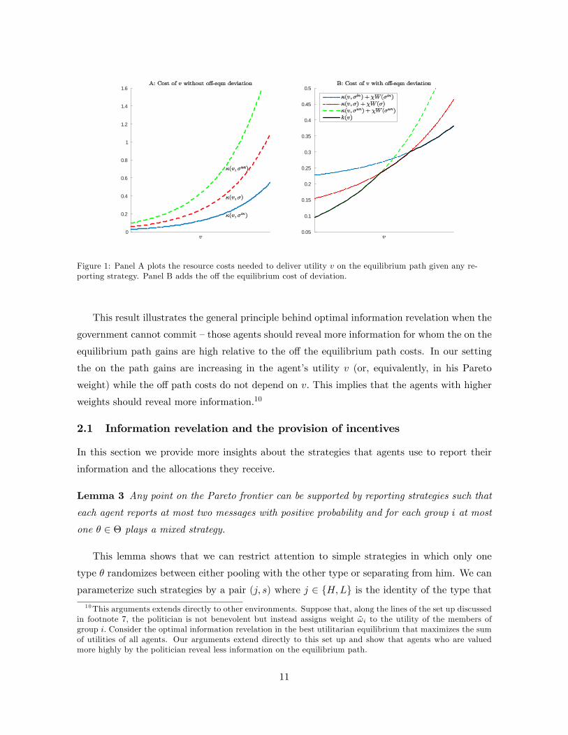
Figure 1 illustrates Proposition 1 graphically. Panel A plots � for three di¤erent reporting

strategies, �in; �un and � =2 �in[�un: The resource gains from better information, � (v; �un)�� (v; �) and � (v; �) � �

�v; �in

�; monotonically increase in v, converge to zero as v ! v and

diverge to in�nity as v ! �v: Panel B adds the o¤ the equilibrium cost of deviation assuming � >

0: Since W��in�> W (�) > W (�un) by Lemma 2, functions f� (�; ~�) + �W (~�)g~�2f�un;�in;�g

must intersect, with less informative functions crossing more informative functions from below.

The lower envelope of these functions characterizes the best reporting strategy for each v:

9 In particular, a = 1 if � 6= 1 and a = 12if � = 1. Observe that if u�t (m; v) is a solution to (13) for given v;

then u�t (m; v) = vu�t (m; 1) if � < 1; u�t (m; v) = �vu�t (m;�1) if � > 1 and u�t (m; v) = 1

2v + u�t (m; 0) if � = 1:

10

0

0.2

0.4

0.6

0.8

1

1.2

1.4

1.6

0.05

0.1

0.15

0.2

0.25

0.3

0.35

0.4

0.45

0.5

Figure 1: Panel A plots the resource costs needed to deliver utility v on the equilibrium path given any re-porting strategy. Panel B adds the o¤ the equilibrium cost of deviation.

This result illustrates the general principle behind optimal information revelation when the

government cannot commit �those agents should reveal more information for whom the on the

equilibrium path gains are high relative to the o¤ the equilibrium path costs. In our setting

the on the path gains are increasing in the agent�s utility v (or, equivalently, in his Pareto

weight) while the o¤ path costs do not depend on v: This implies that the agents with higher

weights should reveal more information.10

2.1 Information revelation and the provision of incentives

In this section we provide more insights about the strategies that agents use to report their

information and the allocations they receive.

Lemma 3 Any point on the Pareto frontier can be supported by reporting strategies such that

each agent reports at most two messages with positive probability and for each group i at most

one � 2 � plays a mixed strategy.

This lemma shows that we can restrict attention to simple strategies in which only one

type � randomizes between either pooling with the other type or separating from him. We can

parameterize such strategies by a pair (j; s) where j 2 fH;Lg is the identity of the type that10This arguments extends directly to other environments. Suppose that, along the lines of the set up discussed

in footnote 7, the politician is not benevolent but instead assigns weight ~!i to the utility of the members ofgroup i: Consider the optimal information revelation in the best utilitarian equilibrium that maximizes the sumof utilities of all agents. Our arguments extend directly to this set up and show that agents who are valuedmore highly by the politician reveal less information on the equilibrium path.

11

separates and s 2 [0; 1] is his probability of separation. In the appendix we show that Lemma3 implies that the cost minimization problem if type L randomizes can be written as

�L (v; s) = minfut(mj)gt2f1;2g;j2fH;Lg

s�L [�1C (u1 (mL)) + �2C (u2 (mL))] (15)

+(�H + (1� s)�L) [�1C (u1 (mH)) + �2C (u2 (mH))]

subject to

v = s�L [�Lu1 (mL) + u2 (mL)] + (1� s)�L [�Lu1 (mH) + u2 (mH)] (16)

+�H [�Hu1 (mH) + u2 (mH)]

and

�Lu1 (mL) + u2 (mL) = �Lu1 (mH) + u2 (mH) : (17)

The cost minimization problem if type H randomizes, �H (v; s) ; is written analogously but

(17) is replaced with

�Hu1 (mL) + u2 (mL) = �Hu1 (mH) + u2 (mH) : (18)

We de�ne WL (s) and WH (s) similarly.

Letnujt (m; v; s)

om;t

be the solution to the minimization problem de�ned by �j (v; s) : Let

vj (mk; v; s) = �kuj1 (mk; v; s) + u

j2 (mk; v; s) be the utility received by type �k:

Proposition 2 (a) Functions �j (v; �) ; �W j (�) ; �huj2 (mL; v; �)� uj2 (mH ; v; �)

i;h

uj1 (mL; v; �)� uj1 (mH ; v; �)i; vj (mj ; v; �) ; �vj (m�j ; v; �) are all decreasing.

(b) �j (v; �) is di¤erentiable and its derivative takes a form @@s�

j (v; s) = �bj (s)C (av) forsome bj (s) : There exist strictly positive ";�" such that bj (s) 2 [";�"] and @

@sWj (s) 2 [";�"] for

all j; s:

Part (a) of Proposition 2 shows how the probability of separation is related to informa-

tiveness and insurance. Strategies with higher probability of separation are more informative

(since �j (v; �) is decreasing andW j (�) is increasing). More informative strategies save resourcesbecause they allow the government to provide better insurance (uj1 (mH ; v; �)�uj1 (mL; v; �) in-creases). The incentive compatibility is preserved by increasing uj2 (mL; v; �)� uj2 (mH ; v; �) aswell. Contracts that incentivize agent j to separate with higher probability also lower that

agent�s utility in favor of the other agent (vj (mj ; v; �) is decreasing, vj (m�j ; v; �) is increasing).Part (b) of Proposition 2 characterizes marginal gains from more informative strategies on

and o¤ the equilibrium path, @@s�

j (v; s) and @@sW

j (s) : One important observation is that the

12

marginal gain from better information is always strictly positive o¤ the equilibrium path. To

see this consider problem (15). The posterior beliefs of the government are bounded away from

each other for any s since Es [�jmL] = �L < 1 � Es [�jmH ] : Thus any marginal increase in the

informativeness of s yields a strictly positive gain. On the other hand, the marginal gain from

better information on the equilibrium path, @@s�

j (v; s) ; becomes unboundedly small as v ! v

and unboundedly large as v ! �v: We then immediately get the following result.

Corollary 1 For any point on the Pareto frontier, there are v�; v+; with v � v� < v+ < �v

(with v < v� if � > 0), such that if vi < v� then ��i is uninformative, and if vi > v+ then ��iis fully informative.

Proof. Since the di¤erence � (v; �un)� ��v; �in

�goes to zero as v ! v and to in�nity as

v ! �v; while W (�un)�W��in�is bounded, full information revelation cannot be optimal for

low values of v (as long as � > 0) and no information revelation cannot be optimal for high

values of v: If any intermediate reporting strategy is optimal, by Lemma 3 it is equivalent to a

strategy where only some type j randomizes between two messages. Since both �j and W j are

di¤erentiable, the optimality condition can be written as @@s�

j (v; s) = � @@sW

j (s) : The bounds

in Proposition 2(b) rule out this possibility for su¢ ciently high and low v:

This proposition shows that for any point v there are some bounds fv�; v+g so that if vi isoutside of these bounds then the optimal strategy is either uninformative or fully informative.

These regions may or may not be empty depending on the point v, although they are always

nonempty provided that fvigi are su¢ ciently di¤erent from each other and � > 0: As we

shall see next, these regions play a key role once we consider a more general class of insurance

mechanisms.

2.2 Stochastic mechanisms and rationing of insurance

So far we focused on deterministic mechanisms: all agents from the same group i were treated

in the same way by the government and received allocations as a function of their group identity

and their reports. Figure 1 suggests that such mechanisms may lead to a non-convex Pareto

frontier. In such cases stochastic insurance mechanisms will further improve welfare. In this

section we extend our analysis to such mechanisms.

Formally we consider the same environment as in the previous section but allow both the

government and the agents to condition their strategies on the realization of an agent-speci�c,

payo¤-irrelevant variable z uniformly distributed on the set Z = [0; 1] :We keep all the notation

parallel to that in the previous section, but use bold letters to emphasize that the variable may

13

depend on z: Thus upri;t;ui;t : M � Z ! R are promises and �nal allocations of the politicianwhile �i : Z � � ! R are the reporting strategies of the agents. The expectation for any

variable x 2 ��M � Z is now de�ned as E�x �R��M�Z x (�;m; z)� (d�)� (dmjz; �) dz:

Our analysis of this game proceeds with minimal changes. Same arguments to the ones

used before show that the sustainability constraint for the politician can be written as

IXi=1

iE�i [�ui;1 + ui;2] �IXi=1

i

ZZW (�i (�jz; �)) dz + U ��; (19)

which is the stochastic analogue of (11). The equilibrium strategies are a solution to the

Lagrangian

Lstoch = minu;�

Xi

i

ZZ

"E�i

"Xt

�tC (ui;t)

����� z#+ �W (�i (�jz; �))

#dz;

where ui (�; z) and �i (�jz; �) are subject to the incentive constraint (6) for all i and z, and theconstraint

vi =

ZZE�i [�ui;1 + ui;2jz] dz for all i:

Stochastic mechanisms improve welfare by relaxing constraint (8). For each realization of

z; the optimalnu�i;1 (�; z) ;u�i;2 (�; z) ;��i (�jz; �)

ois a solution to problem (13) for some vi (z) and

the relationship between vi and vi (z) is given by vi =RZ vi (z) dz: The value of the Lagrangian

satis�es Lstoch=Pi kstoch (vi) i where k

stoch (v) is the convex hull of k (v) de�ned in (14).

The results of the previous section extend directly to stochastic mechanisms using the

following notion of informativeness. Without loss of generality we assume that � is increasing

in z in a sense that z00 � z0 implies that � (�jz00; �) � � (�jz0; �) and say that � is more informativethan ~� if � (�jz; �) � ~� (�jz; �) for all z: We call � fully informative (uninformative) if � (�jz; �)is fully informative (uninformative) for all z: Since the optimal allocations for any ~� (�jz; �) arethe solution to (13) the analysis in Section 2.1 applies to stochastic mechanisms. The results

of Proposition 1 and Corollary 1 extend directly as well. In particular, we have

Corollary 2 Any best PBE is payo¤-equivalent to a PBE with a property that vi00 � vi0 implies

��i00 � ��i0 : There exist v�; v+; with v � v� < v+ < �v (with v < v� if � > 0), such that if

vi < v� then ��i is uninformative, and if vi > v+ then ��i is fully informative.

The main new insight of this section is that stochastic mechanisms may lead to Pareto

improvements and take a particularly simple form.

14

Proposition 3 Suppose � = 1: There is an open set D � R4+ such that if�f�j ; � (�j)gj

�2 D

then for vi 2 [v�; v+] the optimal strategies satisfy ��i (�jz; �) = �un; v�i (z) = v� if z < �zi and

��i (�jz; �) = �in; v�i (z) = v+ if z � �zi; where �zi = v+�viv+�v� : The set D does not depend on the

values of f!i; igi or �:

The proof of this proposition is in the appendix. It shows that whether any strategy

� =2��in; �un

is optimal depends only on the parameters f�i; � (�i)gi ; and not on any other

variables, including the Lagrange multipliers in problem (13). It also provides su¢ cient con-

ditions for f�i; � (�i)gi that ensure that partial pooling is never optimal.11

When the assumptions of Proposition 3 are satis�ed, insurance provision takes a simple

form. Only second best insurance, that requires full information revelation, is provided by the

government but access to this insurance is limited. Low-vi agents receive no insurance, high-vi

agents receive insurance with probability 1, while agents with intermediate values of vi receive

insurance allocated through a lottery. All agents in this intermediate range receive the same

allocations if they win the lottery, but higher values of vi imply better odds of winning the

lottery. One natural interpretation of the lottery is that insurance is rationed.

Consider the implications of Proposition 3 for the case when there is no ex-ante hetero-

geneity across agents and the government maximizes the ex-ante utility of all citizens. This

corresponds to I = 1 in our set up. Some information revelation is optimal in the best equi-

librium for all � > 0 but full information revelation is infeasible if � is not too high. Under

the assumptions of Proposition 3 none of the agents plays a mixed reporting strategy in this

case. Rather, agents are randomly assigned to two groups. Agents in the �rst group reveal full

information about their shock and receive the second best insurance that gives them utility v+:

Agents in the second group reveal no information and receive no insurance obtaining utility of

v� < v+:

Finally, in this section we characterized the e¢ cient insurance arrangements when agents

communicate directly with the government. This is a natural assumption in the context of

many political economy environments. In the Supplementary material we extend our analysis

to environments that involve a mediator, along the lines of Myerson (1982), and show that our

main insights carry over to such economies.

11 In fact, we cojecture that Proposition 3 is stronger as we have not been able to �nd parameters f�i; � (�i)gifor which it is not satis�ed.

15

3 An in�nitely repeated game

In this section we extend our analysis to in�nitely repeated games. We consider a version of

the Atkeson and Lucas (1992) environment in which insurance is provided by a benevolent

government. Our main departure from that model is the assumption that the government

cannot commit.

The economy is populated by a continuum of agents of total measure 1 and the government.

There is an in�nite number of periods, t = 0; 1; 2; ::: The economy is endowed with e units of

a perishable good in each period. An agent�s instantaneous utility from consuming ct units

of the good in period t is given by �tU (ct) where U : R+ ! R is an increasing, strictly

concave, continuously di¤erentiable function. The utility function U satis�es Inada conditions

limc!0 U 0 (c) = 1 and limc!1 U 0 (c) = 0 and it may be bounded or unbounded. Let �u =

limc!1 U (c) ; u = limc!0 U (c) be the bounds (which may be in�nite) of U: Let C � U�1 be

the inverse of the utility function. All agents have a common discount factor �. Let �v = �u1�� ;

v = u1�� be the bounds on the lifetime utility.

The taste shock �t takes values in a �nite set � with cardinality j�j: In this section weassume that �t are i.i.d. across agents and across time, but we relax this assumption in Section

4. Let � (�) > 0 be the probability of realization of � 2 �: We assume that �1 < ::: < �j�j

and normalizeP�2� � (�) � = 1:We use superscript t to denote a history of realizations of any

variable up to period t, e.g. �t = (�0; :::; �t). Let �t��t�denote the probability of realization

of history �t: We assume that types are private information. Each agent belongs to a group

v 2 (v; �v) in period 0 ([v; �v) if utility is bounded below) and the distribution of agents over(v; �v) is denoted by . For now we treat as exogenous following Section 2, but in Section

3.3 we endogenize it when we consider properties of invariant distributions.

Consumption allocations are provided by the government, which is utilitarian but lacks

commitment. Formally we consider an in�nitely repeated game between the government and

a continuum of agents along the lines of Chari and Kehoe (1990) and Chari and Kehoe (1993).

Each period t is divided in two stages. In stage 1 agents transmit information to the government

about their type using a message set M; which for simplicity we assume to be countable. Each

agent sends a report mt 2M about the realization of his type using strategy �t. The reports

are a function of current and past realizations of shocks �t; current and past realizations of

idiosyncratic sunspot variables zt; past reports mt�1; initial group identity v; and the history

of government�s actions that we describe below. Let �ht =�v;mt�1; zt

�and ht =

�v;mt; zt

�be,

respectively, the idiosyncratic histories of agents before and after they submit reports mt; and

let �Ht and Ht be the spaces of all such histories. A reporting strategy �t induces a probability

16

distribution over M denoted by �t��j�ht; �t

�; which also depends implicitly on the history of

government�s actions. We assume that the law of the large numbers holds and the aggregate

distribution of histories ht; denoted by �t; is given by12

��1 (v) = (v) ;

�t�ht�= �t�1

�ht�1

�Pr (zt)

X�t2�t

�t��t��t�mtjht�1; zt; �t

�:

The triple Ht; its Borel sigma algebra, and �t is a probability space.

In stage 2 of each period the government chooses allocations. The allocations are mea-

surable functions ut from Ht into (u; �u) (into [u; �u) if U is bounded below) that satisfy the

feasibility constraint. Using the shorthand notation E�xt =Rxtd�t for any measurable xt; the

feasibility constraint can be written as

E�C (ut) � e for all t: (20)

All variables de�ned above are also functions of aggregate histories. The aggregate histories

include the distribution of reports, � = f�tg1t=0 ; and the distribution of allocations chosen bythe government, u = futg1t=0 : The strategies of the agents and the government are restrictedso that they take the same values for any two aggregate histories that di¤er for a measure zero

of agents. Given this restriction the reporting strategy of any individual agent does not a¤ect

the aggregate allocations in the game.

A PBE consists of strategies of agents and the government and posterior beliefs such that,

at each history of the game, each player chooses his best response given his posterior beliefs

formulated using Bayes�rule. A best PBE is a PBE such that there is no other PBE that gives

higher utility to a set of agents of measure 1, and strictly higher utility to a positive measure

of agents. Without loss of generality we assume that v denotes the lifetime expected utility,

or payo¤ , that the members of group v receive in a best PBE.

3.1 The recursive problem

Our de�nition of equilibrium implies that there is no aggregate uncertainty. Along the equi-

librium path both the aggregate distribution of agents� reports � and the allocations u are

12Strictly speaking, since zt is a continuous variable, �t is de�ned as follows. Let ��1 = : Any Borel set At

of Ht can be represented as a product At = At�1 � Bm � Bz; where At�1 is a Borel set of Ht�1 and Bm,Bzare the mt- and z-sections of some Borel set of Mt � Z: Then �t is de�ned as

�t�At�= �t�1

�At�1

�Pr (zt 2 Bz)

X�t

�t��t��t�BmjAt�1; Bz; �t

�:

17

deterministic sequences. Following standard arguments, government�s equilibrium strategies

are supported by a threat to revert to a PBE that gives the government the lowest utility, which

we call a worst PBE, if the government deviates. Next lemma constructs such an equilibrium.

Lemma 4 In a worst PBE all agents report the same message for all histories��ht; �t

�and

the government allocates U (e) independently of the agents�reports.

Proof. Let �w be a reporting strategy in which the same message is reported for all

histories, let uw be the allocation rule that takes a constant value U (e) for all ht, and let the

government�s posterior beliefs be given by E�w��jht

�= 1 for all ht: It is easy to see that this

triple is consistent with Bayes�rule and constitutes best responses of agents and the government

to each other�s strategies. Therefore it is a PBE. It gives the government payo¤ U(e)1�� : Since the

allocation uw is feasible for any other reporting strategies of the agents, government�s payo¤

must be at least U(e)1�� in any PBE. Therefore, the constructed equilibrium is a worst PBE.

Let � = f�tg1t=0 be a reporting strategy and let � be the induced distribution of reports.The highest payo¤ that the government can achieve in period t is given by a function ~Wt (�t)

de�ned by~Wt (�t) = maxut

E��ut (21)

subject to (20). Therefore the best response constraint of the government can be written as

E�1Xs=t

�s�t�sus � ~Wt (�t) +�

1� �U (e) for all t: (22)

Since each agent�s report does not a¤ect aggregate distributions, agents� incentive con-

straints are

E�

" 1Xt=0

�t�tut

����� v#� E�0

" 1Xt=0

�t�tut

����� v#for all �0; v: (23)

Therefore, any best equilibrium is a solution to

maxu;�

E�1Xt=0

�t�tut (24)

subject to (20), (22), (23), and

E�

" 1Xt=0

�t�tut

����� v#= v: (25)

We start the analysis by simplifying strategies and allocations.

18

Lemma 5 Any best PBE is payo¤ equivalent to a PBE in which �t is independent of �t�1

and for which the following property holds: if there is some w 2 R and histories h0t; h00t suchthat

w = E�

" 1Xs=t

�s�t�sus

�����h0t#= E�

" 1Xs=t

�s�t�sus

�����h00t#;

then �T�mj�h0T ; �T

�= �T

�mj�h00T ; �T

�; uT

��h0T ;mT

�= uT

��h00T ;mT

�for all T > t where

�h0T =�h0t; zt+1;mt+1; :::; zT

�; �h00T =

�h00t; zt+1;mt+1; :::; zT

�for some (zt+1;mt+1; :::; zT ) and

mT :

This lemma is an intermediate step in our recursive characterization of best PBE. It shows

that all the information required to characterize the agents�behavior after any period t can be

summarized in a variable w that captures the agent�s expected continuation payo¤ in period t

along the equilibrium path.

Our analysis of optimal information revelation relies on the recursive formulation of problem

(24). Let (u�;��) be a best PBE and �� be the distribution of histories induced by ��: Let

�wt be the Lagrange multiplier on the feasibility constraint (20) in the maximization problem

(21) when �t = ��t : For any mapping � : �! �(M) let Wt (�) be given by

Wt (�) � maxfu(m)gm2M

X(m;�)2M��

(�u (m)� �wt C (u (m)))� (mj�)� (�) + �wt e: (26)

We use E�Wt as a shorthand forRHt�1�ZWt

��t��jht�1; z; �

��dzd�t�1: The arguments of

Lemma 1 immediately establish the following result.

Lemma 6 (u�;��) is a solution to the maximization problem (24) in which constraint (22) is

replaced with

E�1Xs=t

�s�t�sus � E�Wt +�

1� �U (e) for all t: (27)

Lemma 6 allows us to form a Lagrangian to the constrained maximization problem and

study it using recursive techniques along the lines of our analysis in Section 2. Let��t��t

1t=0

and��t��t

1t=0

be the Lagrange multipliers on (20) and (27), respectively. The Lagrangian

to the constrained maximization problem can be written as (see, e.g. Marcet and Marimon

(2009) or Chapter 20.4 in Ljungqvist and Sargent (2012))

L = maxu;�

E�1Xt=0

��t [�tut � �tC (ut)� �tWt] (28)

19

subject to (23) and (25), where ��t = �t�1 +

Pts=0 �

�s

�; �t = �t��t =��t; and �t = �t��t =��t: Let

�t � ��t=��t�1 be the e¤ective discount factor. By de�nition �t � � with strict inequality if and

only if constraint (27) binds in period t:

Problem (28) is the in�nite period analogue of (12). Our analysis proceeds similarly to

that in Section 2. De�ne

kt (v) �1��tmaxu;�

E�

" 1Xs=0

��t+s��sus��t+sC (us)� �t+sWt+s

������ v#

(29)

subject to (23) and (25). The Lagrangian (28) satis�es L =R��0k0 (v) d :

Lemma 7 Wt satis�es all the properties of Lemma 2.

kt is continuous, concave and di¤erentiable with limv!�v k0t (v) = �1: If utility is un-bounded below then limv!v k0t (v) = 1; if utility is bounded below then limv!v k0t (v) � 1 with

limv!v k0t (v) =1 if lim sup�t > 0:

It is easy to write (29) recursively. Suppose (u�;��) is a best PBE, which without loss of

generality satis�es the properties of Lemma 5. For any ht�1 let v = E���P1

s=t �s�t�su�sjht�1

�.

Then�u�t�ht�1;mt; zt

�;��t

�mtjht�1; zt; �t

�mt;�t;zt

is a solution to

kt (v) = maxu;w;�

ZZ

24X�;m

� (�)� (mjz; �)h�u (m; z)� �tC (u (m; z)) + �t+1kt+1 (w (m; z))

i� �tW (� (�jz; �))

35 dz(30)

subject to

v =

ZZ

X�;m

� (�)� (mjz; �) [�u (m; z) + �w (m; z)] dz; (31)

Xm

� (mjz; �) [�u (m; z) + �w (m; z)] �Xm

�0 (mjz; �) [�u (m; z) + �w (m; z)] for all z; �;�0:

(32)

To characterize the properties of e¢ cient information revelation it is useful to separate the

maximization problem (30) into two components. Let t (v) � k0t (v) : For � : �! �(M) and

for any x :M ��! R de�ne E�x as in Section 2 and let

�t (v; �) � maxfu(m);w(m)gm2M

E�h(1� t (v)) �u� �tC (u) + �t+1kt+1 (w)� t (v)�w

i+ t (v) v

(33)

subject to

�u (m�) + �w (m�) � �u (m) + �w (m) for all �;m; (34)

20

and

� (mj�) [(�u (m�) + �w (m�))� (�u (m) + �w (m))] = 0 for all �;m; (35)

where m� is any message such that � (m�j�) > 0. Let (uv;wv;�v) denote a solution to (30).

Similarly, we use (uv;�; wv;�) to denote a solution to (33). The relationship between �t and kt

is given by the following lemma.

Lemma 8 kt satis�es

kt (v) = max�f�t (v; �)� �tWt (�)g : (36)

Moreover, (uv (�; z) ;wv (�; z)) is a solution to (33) with � = �v (�jz; �) and �v (�jz; �) is a solu-tion to (36) for all z.

We use �v to denote a solution to (36). Problem (33) has a similar structure to the standard

recursive characterization in dynamic contracting models with commitment (e.g., Atkeson and

Lucas (1992), Farhi and Werning (2007), Sleet and Yeltekin (2006)), except that it allows

agents to send noisy information about their type. When the principal (the government in our

setting) cannot commit, more precise information carries costs, which are captured by �tWt:

The optimal information revelation is characterized by (36). When the cost of information

revelation is absent, �t = 0; full information revelation is optimal, as in standard principal-

agent models.

Before we proceed we comment on how the cardinality of the message set a¤ects the payo¤s

in best PBE. Larger message sets weakly increase welfare because it is possible to replicate

the payo¤s of a smaller message set with a larger one. To see this, take any message space M 0

and consider an alternative message space M 00 constructed by adding additional messages to

M 0. The government can always give the lowest payo¤ to any agent who reports a message

m 2M 00nM 0 and, thus, ensure that in equilibrium messages m 2M 00nM 0 are not played. The

next lemma shows that the highest welfare can be attained with a �nite message space. Let

M� be a set with 2j�j � 2 elements m1; :::;m2j�j�2:

Lemma 9 Any payo¤ of a best PBE in a game that uses message set M can be attained in a

game that uses message set M�:

In particular, Lemma 9 implies that there is no gain from allowing the government to

�pre-commit�to getting coarser information by choosing a smaller message set. For example,

suppose we introduced a preliminary stage in every period of our dynamic game in which the

government can choose the optimal message set. By Lemma 9, without loss of generality the

government would simply choose M�: For concreteness, we assume for the rest of the paper

that M =M�.

21

3.2 Characterization

In this section we characterize properties of e¢ cient information revelation. In addition to

uninformative and fully informative strategies de�ned in Section 2 we say that strategy � reveals

full information about type j if there is ~M �M� such that ��~M j�j

�= 1 and E�

h�j ~M

i= �j :

The same de�nition applies to � if � (�jz; �) reveals full information about type j for all z:Some of our results require the following assumption.

Assumption 1 (decreasing absolute risk aversion) U is twice continuously di¤erentiable

and

limc!1

U 00 (c) =U 0 (c) = 0: (37)

We start our analysis by assuming that j�j = 2. In this case many of the results of Section 2extend directly. For example, the same arguments used in Lemma 3 show that we can focus on a

message space containing only two messages with at most one type randomizing between them.

Similarly, we can extend most of the comparative statics of Proposition 2(a). In particular, a

higher probability of separation increases both �t (v; �) and Wt (�). Moreover, a higher prob-

ability of separation allows the government to provide better insurance (uv;� (mH)�uv;� (mL)

increases). The incentive compatibility is preserved by increasing wv;� (mL) � wv;� (mH) as

well. The next Proposition is the analogue of Corollaries 1 and 2.

Proposition 4 Suppose j�j = 2:(a). Suppose either utility is bounded below or �t+1 > 0. If �t > 0 then there exists v

�t > v

such that �v 2 �un and �v is uninformative for all v � v�t .

(b). If Assumption 1 is satis�ed then there exists v+t < �v such that �v 2 �in �v is fullyinformative for all v � v+t .

The proof of this proposition is in the appendix, here we sketch the main steps. Suppose

that the probability of separation is interior, so that some type j plays �v (mj j�j) 2 (0; 1).Consider an uninformative strategy �un (m�j j�j) = �un (m�j j��j) = 1 and a fully informativestrategy �in (mj j�j) = �in (m�j j��j) = 1: Optimality of �v implies the following �rst order

conditions:

�t@Wt (�v)

@�un=

@�t (v; �v)

@�un; (38)

�t@Wt (�v)

@�in=

@�t (v; �v)

@�in: (39)

The expressions on the left hand side of (38) and (39) capture the marginal cost o¤ the

equilibrium path from changing informativeness of agents�strategies. As in Proposition 2(b),

22

the derivatives of Wt are �nite and non-zero. The expressions on the right hand side of (38)

and (39) capture the marginal gain on the equilibrium path from changing informativeness

of agents� strategies. Under the assumptions of Proposition 4, the marginal gain of better

information on path becomes arbitrarily small as v approaches v and arbitrarily large as v

approaches �v. This implies that an interior probability of separation is suboptimal for low and

high values of v; and that high-v agents play fully informative strategies while low-v agents

play uninformative strategies.

Now consider the case with j�j > 2. Part (a) of Proposition 4 extends to this case withoutany additional considerations. The reason for it is that the marginal gain of more information

disappears as v ! v for any cardinality of �: The result of full information revelation for

su¢ ciently high v requires extra assumptions. In general, when j�j > 2 it might be optimal tobunch some types together and give them the same allocations even in the second best problem,

that has no cost of information revelation. In such situations revealing full information is

strictly suboptimal if �t > 0: Part (b) provides su¢ cient conditions that ensure that it is not

optimal to bunch type � in the second best environment and show that under such conditions

�v reveals full information about that type if v is su¢ ciently large.

Proposition 5 For any j�j;(a). Suppose either utility is bounded below or �t+1 > 0: If �t > 0 then there exists v

�t > v

such that �v is uninformative for all v � v�t .

(b). If Assumption 1 is satis�ed, then there exists v+t < �v such that �v reveals full informa-

tion about �1 for all v � v+t : If, in addition, ���j�j�1

� ��j�j � �j�j�1

�>����j�j�1

�+ �

��j�j�� �

�j�j�1 � �j�j�2�

and 1 + �1 � �j�j � 0; then �v reveals full information about �j�j for all v � v+t :

Moreover, if U (c) is CES with � 2 (0; 1) and � satis�es the no-bunching condition

� (�n�1) [�n � �n�1]� (�n�1 � �n�2)j�jX

i=n�1� (�i) � 0 for all n > 2; (40)

then �v is fully informative for all v � v+t :

3.3 Invariant distribution

In our analysis so far we took the initial distribution of utilities as given. Any is as-

sociated with Lagrange multipliers f�t; �t; �wt g1t=0 which, together with the Bellman equa-

tions (33) and (36), can be used to recover the equilibrium strategies that support : More-

over, any induces a sequence of distributions of continuation utilities of the agents, vt =

E���P1

s=0 �s�t+su

�t+s

��ht�1� ; which we denote by t with 0 = : We say that is invariant

23

if f�t; �t; �wt ; tg1t=0 do not depend on t: This also implies that in an invariant distribution

�t = �= (1� �) does not depend on t:

Lemma 10 In any invariant distribution � > 0; � > � and in each period a positive measure

of agents does not play uninformative strategies. Continuation utilities are mean-reverting:

�

�E�v

�k0 (wv)

�= k0 (v) : (41)

If 1+�1��j�j � 0, then there is some w > v such that wv (m; z) � w for all v 2 supp ( ) n fvgwith ww (m; z) > w for some m; z:

This lemma shows that in any invariant distribution the sustainability constraint (22)

binds. If it did not, our economy would be isomorphic to Atkeson and Lucas (1992). In

that environment immiseration (the distribution that assigns mass 1 on v) is the only feasible

invariant distribution, but such distribution violates (27). The binding constraint (27) also

implies that agents� continuation utilities exhibit mean-reversion (41); that in each period

some agents reveal information to the government; and that, if any agent enters the region of

continuation utilities in which it is optimal to reveal no information, he must exit it in �nite

time. Finally, as long as the dispersion of shocks is not too high, there is a re�ecting lower

bound w below which agents�continuation utilities do not fall if they start above it.13

Figure 2 illustrates the policy functions in an invariant distribution.14 The optimal report-

ing strategy �v follows the same patterns as those in Proposition 3. �v (�jz; �) is either fullyinformative or uninformative for all realizations of (v; z). Agents reveal no information and

receive no insurance with probability 1 for all v � v� (v� is shown by the �rst dashed line in

panel A) and reveal full information and receive the second best insurance with probability 1

for all v � v+ (v+ is shown by the second dashed line in panel A). Finally, insurance is rationed

if v 2 (v�; v+). In this case the agent receives allocations associated with v+ and reveals fullinformation with probability v+�v

v+�v� and receives no insurance, reveals no information, and

obtains utility v� with probability v�v�v+�v� .

The typical dynamics of vt in the invariant distribution can be seen from panel B. Consider

an agent whose initial lifetime utility v0 equals the lowest v in the support of the invariant

distribution. The continuation utility of such agent initially grows deterministically over time.

13There exist invariant distributions that put a positive mass on v; which is an absorbing state. The probabilityof reaching this point from any other point in the support of the invarinant point is zero.14To compute this �gure we set U (c) = ln (c) ; � = 0:53; e = 1 and � = f0:8; 1:2g with both shocks occuring

with equal probability. These assumptions imply that �w = 1. To �nd an invariant distribution, we computethe stationary distribution implied policy functions to (33) and (36) and iterate on (�; �) until the stationarydistribution satis�es constraints (20) and (22).

24

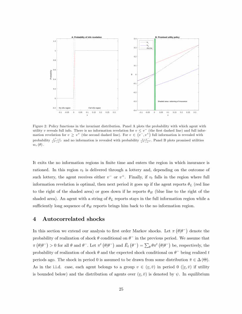
­0.1 ­0.05 0 0.05 0.1 0.15 0.2 0.25 0.3v

­0.4

­0.3

­0.2

­0.1

0

0.1

0.2

0.3

0.4

w

B: Promised utility policy

Shaded area: rationing of insurance

wL

wH

45o line

­0.1 ­0.05 0 0.05 0.1 0.15 0.2 0.25 0.3v

­0.2

0

0.2

0.4

0.6

0.8

1

1.2

Prob

abilit

y

A: Probability of info revelation

Full info regionNo info region

Figure 2: Policy functions in the invariant distribution. Panel A plots the probability with which agent withutility v reveals full info. There is no information revelation for v � v� (the �rst dashed line) and full infor-mation revelation for v � v+ (the second dashed line). For v 2

�v�; v+

�full information is revealed with

probability v+�vv+�v� and no information is revealed with probability v�v�

v+�v� : Panel B plots promised utilitieswv (�) :

It exits the no information regions in �nite time and enters the region in which insurance is

rationed. In this region vt is delivered through a lottery and, depending on the outcome of

such lottery, the agent receives either v� or v+. Finally, if vt falls in the region where full

information revelation is optimal, then next period it goes up if the agent reports �L (red line

to the right of the shaded area) or goes down if he reports �H (blue line to the right of the

shaded area). An agent with a string of �L reports stays in the full information region while a

su¢ ciently long sequence of �H reports brings him back to the no information region.

4 Autocorrelated shocks

In this section we extend our analysis to �rst order Markov shocks. Let ���j��

�denote the

probability of realization of shock � conditional on �� in the previous period. We assume that

���j��

�> 0 for all � and ��: Let �t

��j��

�and �Et

����=P� ��

t��j��

�be, respectively, the

probability of realization of shock � and the expected shock conditional on �� being realized t

periods ago. The shock in period 0 is assumed to be drawn from some distribution �� 2 �(�).As in the i.i.d. case, each agent belongs to a group v 2 (v; �v) in period 0 ([v; �v) if utilityis bounded below) and the distribution of agents over (v; �v) is denoted by . In equilibrium

25

members of group v receive lifetime expected utility v.

Many arguments when types are Markov are direct extensions of our previous analysis.

We brie�y lay out the arguments here and leave the details in Supplementary material. We

assume throughout that agents are required to send messages from a �nite message space M .

Given a reporting strategy �, let pt : Ht ! �(�) denote the government�s belief about the

agent�s shock conditional on history ht. These posteriors are generated recursively starting

from p0 = �� and using Bayes rule

pt��jht�1; zt;mt

�=�t�mtjht�1; zt; �

�P�� �

��j��

�pt�1

���jht�1

�P�;�� �t (mtjht�1; zt; �)�

��j��

�pt�1

���jht�1

� ; (42)

for all ht�1; zt; and mt for which the expression is well-de�ned. For any x : Ht � � !R, the expectation of x conditional on some history ht�1 2 Ht�1 and type �� 2 � is

E��xjht�1; ��

�=RM�Z

P� x�ht�1; z;m; �

��t (dmjz; �)�

��j��

�dz. Similarly, the uncondi-

tional expectation is E� [x] =RHt�1

P�� E�

�xjh; ��

�pt�1

���jh

�d�t�1.

It is immediate to extend Lemma 4 to Markov shocks and show that in the worst equi-

librium agents play uninformative strategies. Unlike the i.i.d. case, however, the payo¤ in

that equilibrium depends on the beliefs of the government. The maximum payo¤ that the

government can achieve in any period t is given by

~Wt (�t) � maxfut+s(h)gh2Ht;s�0

E�

" 1Xs=0

�s �Esut+s

#(43)

subject to the feasibility constraints (20).

Similarly to the i.i.d. case, we �rst bound ~Wt (�t) with a function that is linear in �t�1: Let��wt;t+s

1s=0

be the sequence of Lagrange multipliers on (20) in the maximization problem that

de�nes ~Wt (��t ) : Let � : �! �(M) ; the expectation of the random variable x : M ��! R

conditional on some �� 2 � is now E��xj��

�=

Pm;�2M��

x (m; �)� (mj�)���j��

�: For any

p 2 �(�), let Wt (�; p) be de�ned as

Wt (�; p) � maxfut+s(m)gs�0

X��

E�

" 1Xs=0

�s��Esut+s � C (ut+s) + �wt;t+se

������ ��#p����: (44)

Wt (�; p) is the generalization of (26) to the Markov case and p represents the beliefs that the

government holds about the agents�types in period t� 1: ~Wt (�t) is bounded by

~Wt (�t) �ZHt�1�Z

Wt

��t��jht�1; z; �

�;pt�1

�ht�1

��dzd�t�1;

with equality if �t = ��t , �t = ��t , pt�1 = p

�t�1, where fp�t g are the beliefs corresponding to

��: This bound can then be used to replace the incentive constraint for the government with

a constraint that is linear in �t�1.

26

Replacing the incentive constraint for the government, in turn, enables us to use Lagrangian

methods and solve the problem recursively. In particular, we �rst de�ne a Lagrangian and a

value function kt��!v ; p� ; where now �!v =

��!v (�1) ; :::;�!v ��j�j�� is a vector of continuationutilities, which are the analogues of (28) and (29), respectively. We then rewrite the value

function recursively extending the techniques of Fernandes and Phelan (2000). For any x :

M � � � Z ! R let E��xj��

�=RZ

Pm;� �

��j��

�� (mjz; �)x (m; �; z) dz: Also, let u;�;p :

M � Z ! R and �!w :M � Z ��! R. The value function kt��!v ; p� satis�es

kt��!v ; p� = max

(u;�!w;�;p0)

X��

p����E�h�u� �tC (u) + �t+1kt+1

��!w ;p0� j��i��t Z Wt (� (�jz; �) ; p) dz

(45)

subject to�!v����= E�

��u+ ��!w (�; �; �) j��

�for all ��; (46)

E���u+ ��!w (�; �; �) j�; z

�� E�0

��u+ ��!w (�; �; �) j�; z

�for all z; �;�0 (47)

and

p0 (�jm; z)

24X�;��

� (mjz; �)���j��

�p����35 = � (mjz; �)X

��

���j��

�p����: (48)

Constraints (46) and (47) are the analogues of (31) and (32) in the i.i.d. case. The key

di¤erence is that realization of shock � in the current period a¤ects the expected utility of

an agent from the future consumption stream. Thus, the recursive formulation assigns a

continuation utility for each possible realization of �� 2 �: The probability measure p keepstrack of the evolution of the posterior beliefs of the government. When �t = 0 and agents play

fully informative strategy, p assigns probability 1 to one of the values of � and the Bellman

equation (45) simpli�es to the recursive formulation of Fernandes and Phelan (2000). We

conclude this section by a version of Proposition 5(a) for Markov shocks, which we prove in

Supplementary material.

Proposition 6 Suppose utility is bounded below (wlog by 0) and �t > 0. Let ��!v ;p be a solution

to (45), then lim�!v!0 Pr���!v ;p 2 �un

�= 1, uniformly in p.

5 Final remarks

In this paper we took a step towards developing of theory of social insurance in a setting in

which the principal cannot commit. We focused on the simplest version of no commitment that

involves a direct, one-shot communication between the principal and the agents, and showed

27

how such model can be incorporated into the standard recursive contracting framework with

relatively few modi�cations. The natural extension of this approach is to incorporate it into

richer models of social insurance cited in the introduction. This would allow one to explore

how the allocations in best equilibria can be decentralized through a system of taxes and

transfers, for example along the lines of Albanesi and Sleet (2006). Our methods should also

be applicable to other principal-agent environments in which the principal interacts with a

large number of agents and cannot commit, such as models of regulation, employer-employee

relationships, bargaining and trading with private information.

References

Acemoglu, D. (2003): �Why not a political Coase theorem? Social con�ict, commitment,

and politics,�Journal of Comparative Economics, 31(4), 620�652.

Acemoglu, D., M. Golosov, and A. Tsyvinski (2010): �Dynamic Mirrlees Taxation under

Political Economy Constraints,�Review of Economic Studies, 77(3), 841�881.

Aiyagari, S. R., and F. Alvarez (1995): �E¢ cient Dynamic Monitoring of Unemployment

Insurance Claims,�Mimeo, University of Chicago.

Akerlof, G. A. (1978): �The Economics of "Tagging" as Applied to the Optimal Income

Tax, Welfare Programs, and Manpower Planning,�The American Economic Review, 68(1),

pp. 8�19.

Albanesi, S., and C. Sleet (2006): �Dynamic optimal taxation with private information,�

Review of Economic Studies, 73(1), 1�30.

Atkeson, A., and R. E. Lucas (1992): �On E¢ cient Distribution with Private Information,�

Review of Economic Studies, 59(3), 427�453.

Besley, T., and S. Coate (1998): �Sources of Ine¢ ciency in a Representative Democracy:

A Dynamic Analysis,�American Economic Review, 88(1), 139�56.

Bester, H., and R. Strausz (2001): �Contracting with Imperfect Commitment and the

Revelation Principle: The Single Agent Case,�Econometrica, 69(4), 1077�98.

Bisin, A., and A. Rampini (2006): �Markets as bene�cial constraints on the government,�

Journal of Public Economics, 90(4-5), 601�629.

28

Chari, V. V., and P. J. Kehoe (1990): �Sustainable Plans,�Journal of Political Economy,

98(4), 783�802.

(1993): �Sustainable Plans and Debt,�Journal of Economic Theory, 61(2), 230�261.

Clementi, G. L., and H. A. Hopenhayn (2006): �A Theory of Financing Constraints and

Firm Dynamics,�The Quarterly Journal of Economics, 121(1), 229�265.

Cole, H. L., and N. Kocherlakota (2001): �Dynamic Games with Hidden Actions and

Hidden States,�Journal of Economic Theory, 98(1), 114 �126.

Dovis, A. (2009): �E¢ cient Sovereign Default,�Mimeo, Penn State.

Farhi, E., C. Sleet, I. Werning, and S. Yeltekin (2012): �Non-linear Capital Taxation

Without Commitment,�Review of Economic Studies, 79(4), 1469�1493.

Farhi, E., and I. Werning (2007): �Inequality and Social Discounting,�Journal of Political

Economy, 115(3), 365�402.

(2013): �Insurance and Taxation over the Life Cycle,�Review of Economic Studies,

80(2), 596�635.

Fernandes, A., and C. Phelan (2000): �A Recursive Formulation for Repeated Agency

with History Dependence,�Journal of Economic Theory, 91(2), 223�247.

Freixas, X., R. Guesnerie, and J. Tirole (1985): �Planning under Incomplete Informa-

tion and the Ratchet E¤ect,�Review of Economic Studies, 52(2), 173�91.

Golosov, M., M. Troshkin, and A. Tsyvinski (2016): �Redistribution and Social Insur-

ance,�American Economic Review, 106(2), 359�86.

Golosov, M., and A. Tsyvinski (2006): �Designing optimal disability insurance: A case

for asset testing,�Journal of Political Economy, 114(2), 257�279.

Golosov, M., A. Tsyvinski, and I. Werning (2006): �New dynamic public �nance: A

user�s guide,�NBER Macroeconomics Annual, 21, 317�363.

Golosov, M., A. Tsyvinski, and N. Werquin (2013): �Recursive Contracts and Endoge-

nously Incomplete Markets,�working paper.

Green, E. J. (1987): �Lending and the Smoothing of Uninsurable Income,� in Contractual

Arrangements for Intertemporal Trade, ed. by E. C. Prescott, and N. Wallace. University of

Minnesota Press., Minneapolis.

29

Hopenhayn, H. A., and J. P. Nicolini (1997): �Optimal Unemployment Insurance,�Jour-

nal of Political Economy, 105(2), 412�38.

Kocherlakota, N. (2010): The New Dynamic Public Finance. Princeton University Press,

USA.

Kydland, F. E., and E. C. Prescott (1977): �Rules Rather Than Discretion: The In-

consistency of Optimal Plans,�Journal of Political Economy, University of Chicago Press,

85(3), 473�91.

Laffont, J.-J., and J. Tirole (1988): �The Dynamics of Incentive Contracts,�Economet-

rica, 56(5), 1153�75.

Lindbeck, A., and J. W. Weibull (1987): �Balanced-Budget Redistribution as the Out-

come of Political Competition,�Public choice, 52(3), 273�297.

Ljungqvist, L., and T. J. Sargent (2012): Recursive Macroeconomic Theory, Third Edi-

tion. MIT Press.

Luenberger, D. (1969): Optimization by Vector Space Methods. Wiley-Interscience.

Marcet, A., and R. Marimon (2009): �Recursive Contracts,�Mimeo, European University

Institute.

Milgrom, P., and I. Segal (2002): �Envelope Theorems for Arbitrary Choice Sets,�Econo-

metrica, 70(2), 583�601.

Mirrlees, J. (1971): �An Exploration in the Theory of Optimum Income Taxation,�Review

of Economic Studies, 38(2), 175�208.

Myerson, R. B. (1982): �Optimal Coordination Mechanisms in Generalized Principal-Agent

Problems,�Journal of Mathematical Economics, 10(1), 67�81.

Phelan, C., and R. M. Townsend (1991): �Computing Multi-period, Information-

Constrained Optima,�Review of Economic Studies, Wiley Blackwell, 58(5), 853�81.

Roberts, K. (1984): �The Theoretical Limits of Redistribution,�Review of Economic Studies,

51(2), 177�95.

Rockafellar, R. (1972): Convex Analysis, Princeton mathematical series. Princeton Uni-

versity Press.

30

Royden, H. (1988): Real Analysis, Mathematics and statistics. Macmillan.

Scheuer, F., and A. Wolitzky (2014): �Capital Taxation under Political Constraints,�

NBER Working Paper 20043.

Shimer, R., and I. Werning (2015): �E¢ ciency and Information Transmission in Bilateral

Trading,�Working Paper 21495, National Bureau of Economic Research.

Skreta, V. (2006): �Sequentially Optimal Mechanisms,�Review of Economic Studies, 73(4),

1085�1111.

(2015): �Optimal auction design under non-commitment,�Journal of Economic The-

ory, 159, Part B, 854 �890.

Sleet, C., and S. Yeltekin (2006): �Credibility and endogenous societal discounting,�

Review of Economic Dynamics, 9(3), 410�437.

(2008): �Politically credible social insurance,�Journal of Monetary Economics, 55(1),

129�151.

Song, Z., K. Storesletten, and F. Zilibotti (2012): �Rotten Parents and Disciplined

Children: A Politico-Economic Theory of Public Expenditure and Debt,� Econometrica,

80(6), 2785�2803.

Stantcheva, S. (2014): �Optimal Taxation and Human Capital Policies over the Life Cycle,�

working paper.

Thomas, J., and T. Worrall (1990): �Income Fluctuation and Asymmetric Information:

An Example of a Repeated Principal-agent Problem,�Journal of Economic Theory, 51(2),

367�390.

Topkis, D. (2011): Supermodularity and Complementarity, Frontiers of Economic Research.

Princeton University Press.

Yared, P. (2010): �A dynamic theory of war and peace,� Journal of Economic Theory,

145(5), 1921�1950.

31

6 Appendix

6.1 Proofs of Section 2

Proof of Lemma 2. It is immediate that the feasibility constraint (4) binds for any � and

therefore �w > 0: The �rst order condition to (9) gives

C 0 (uw (m)) =1

�wE� [�jm] 2

��L�w

;�H�w

�(49)

for all m sent with positive probability, therefore such uw (m) lie in a compact set. Since

messages sent with zero probability do not a¤ect the value of W; uw (m) can be restricted to

lie in a compact set for all m: The theorem of the maximum then implies thatW is continuous.

For any �0; �, and � 2 [0; 1] de�ne �� = (1� �)� + ��0:

W (��) = maxu

�Xm;�

[�u (m)� �wC (u (m))]�0 (mj�)� (�)

+ (1� �)Xm;�

[�u (m)� �wC (u (m))]� (mj�)� (�) + �w

� �maxu

Xm;�

[�u (m)� �wC (u (m))]�0 (mj�)� (�)

+ (1� �)maxu

Xm;�

[�u (m)� �wC (u (m))]� (mj�)� (�) + �w

= �W��0�+ (1� �)W (�) ;

which establishes convexity. Note that for any collection X of functions x :M ! R; the familyfE��xgx2X is equidi¤erentiable at any � 2 [0; 1) since the expectation is linear in �: Therefore,the derivative @W (�)

@�0 exists by Theorem 3 in Milgrom and Segal (2002) and

@W (�)

@�0= E�0 [�uw0 (m)� �wC (uw0 (m))]� E� [�uw0 (m)� �wC (uw0 (m))] �W

��0��W (�) ;

(50)

where uw� is a solution to W (��) for � > 0 and uw0 (m) = lim�!0 uw� (m) :

15

To show that W (�) achieves its minimum if and only if � is uninformative, let uun be the

optimal allocation corresponding to an uninformative strategy, which without loss of generality

15The problem that de�nes W; (9), is strictly convex and, therefore, the solution uw� (m) is unique foreach m sent with positive probability by ��: The de�nition of uw0 pins down the values of uw0 (m) for whichP

� �� (mj�)� (�) > 0 for � > 0 and lim�!0

P� �� (mj�)� (�) = 0:

32

satis�es C 0 (uun (m)) = 1=�w for all m: For any �

W (�)�W (�un)

= maxu

Xm;�

[(�u (m)� �wC (u (m)))� (�uun � �wC (uun))]� (mj�)� (�)

= maxu

Xm

f(E� [�jm]u (m)� �wC (u (m)))� (E� [�jm]uun � �wC (uun))g X

�

� (mj�)� (�)!:

The expression in curly bracket is non-negative, which implies that W (�) �W (�un) for all �:

If � =2 �un then C 0 (uw (m)) 6= 1=�w for at least one m sent with positive probability. For such

m the expression in the curly brackets is strictly positive so that W (�) > W (�un) if � =2 �un.To show that W (�) achieves its maximum if and only if � is fully informative, take any

� =2 �in. By de�nition there must exist some messagem sent with positive probability such that

E� [�jm] 6= �j for j 2 fL;Hg. By (49) the optimal allocation for such m satis�es C 0 (uw (m)) 6=�j=�

w for j 2 fL;Hg: Let uin be the optimal allocation corresponding to some �in. It satis�edC 0�uin (m)

�= �j=�

w; j 2 fL;Hg for all m sent with positive probability. By strict convexity

of C the optimal allocation must be unique and therefore W��in�> W (�) for all � =2 �in.

We �rst prove a preliminary result that is useful in the proof of both Lemma 3 and of the

results in Section 3.2.

Lemma 11 Any point on the Pareto frontier can be supported by reporting strategies such that

all agents report one of three messages, with each � 2 f�L; �Hg randomizing between at mosttwo messages and with at most one message reported with positive probability by both �.

Proof. Fix any group i and let (u�1; u�2; �

�) be a best equilibrium strategy for that group.

We can partition M into four subset: (i) a subset ML that consists of messages reported with

positive probability by type �L and reporting which gives strictly lower utility to type �H ; i.e.

there exists a message m 2M such that

�Hu�1 (m) + u

�2 (m) > �Hu

�1

�m0�+ u�2 �m0� for all m0 2ML;

(ii) a subset MH de�ned analogously for �H ; (iii) a subset MHL that consists of messages

reported with positive probability by either �H or �L and for which

�u�1 (m) + u�2 (m) � �u�1

�m0�+ u�2 �m0� for all � 2 �;m 2MHL; m

0 2M ; (51)

(iv) and a subset M? containing all other messages.

Consider the subsetML: Bayes�rule implies E�� [�jm] = �L for anym 2ML: If (u�1 (m) ; u�2 (m))

take the same values for all m 2 ML then an alternative strategy of reporting any m 2 ML

33

with probability 1 gives the same allocations, the same payo¤ on equilibrium path, and by

(49) also the same payo¤ o¤ the equilibrium path. Thus, this alternative strategy is payo¤

equivalent to the original strategy. We now rule out the possibility that (u�1 (m0) ; u�2 (m

0)) 6=(u�1 (m

00) ; u�2 (m00)) for somem0;m00 2ML: Let (u�1 ; u

�2 ) = � (u�1 (m

0) ; u�2 (m0))+(1� �) (u�1 (m00) ; u�2 (m

00))

for � 2 (0; 1) : (u�1 ; u�2 ) gives the same utility to �L as (u�1 (m0) ; u�2 (m0)) and (u�1 (m

00) ; u�2 (m00))

and strictly lower utility to type �H than any m000 2 MH [MHL: (u�1; u

�2) must be a solution

to the minimization problem (13) for (vi; ��) : Since the objective function in (13) is strictly

convex, replacing (u�1 (m0) ; u�2 (m

0)) and (u�1 (m00) ; u�2 (m

00)) with (u�1 ; u�2 ) gives a strictly lower

value of the objective function, contradicting the optimality of (u�1; u�2) : Analogous arguments

apply to MH :

Consider the subsetMHL and suppose � > 0 (otherwise the result follows directly from the

standard revelation principle). Condition (51) implies that (u�1 (m) ; u�2 (m)) takes the same

values for all m 2MHL: If E�� [�jm] also takes the same value for any m 2MHL then we can

replace the subset MHL with one message. We next rule out that E�� [�jm0] 6= E�� [�jm00] for

some m0;m00 2MHL.

Fix any m 2 MHL: Consider an alternative strategy �0 that coincides with �� except for

�0 (mj�) =Pm2MHL

�� (mj�), �0 (m0j�) = 0, for allm0 2MHL; m0 6= m, and all �: The strategy

pro�le �� = (1� �)�0 + ��� satis�es (6) and (8) for any � 2 [0; 1] : Since (u�1 (m) ; u�2 (m))takes the same value for all m 2 MHL; the optimality condition for (14) can be written as@W (��)@�0 � 0; where the derivative exists by Lemma 9. From (50),

0 � @W (��)

@�0=

X�;m2MHL

(�uw(m)� �wC(uw(m)))�0 (mj�)� (�)

�X

�;m2MHL

(�uw(m)� �wC(uw(m)))�� (mj�)� (�)

= (E�0 [�jm]uw(m)� �wC(uw(m)))X�

�0 (mj�)� (�)

�X

m2MHL

(E�� [�jm]uw(m)� �wC(uw(m))) X

�

�� (mj�)� (�)!:

By construction,

E�0 [�jm] =P� ��

0 (mj�)� (�)P� �

0 (mj�)� (�) =P�;m2MHL

��� (mj�)� (�)P�;m2MHL

�� (mj�)� (�) = E�� [�jMHL] :

Therefore, the expression above can be re-written as

E�� [�jMHL]uw(m)� �wC(uw(m)) � E�� [(E�� [�jm]uw(m)� �wC(uw (m)))jMHL] :

34

The expression on the right hand side does not depend on m: The expression on the left

hand side holds for all m 2MHL: Multiply both sides byP� �

�(mj�)�(�)P�;m2MHL

��(mj�)�(�) and sum across

all m 2MHL to get

E�� [�jMHL]E�� [uw(m)jMHL] � E�� [(E�� [�jm]uw(m))jMHL] ;

which implies that cov (E�� [�jm] ; uw(m)) � 0: On the other hand, (49) implies that uw (m)

is monotonically increasing in E�� [�jm] ; thus, cov (E�� [�jm] ; uw(m)) � 0: The two conditionscan be satis�ed only if E�� [�jm] takes the same values for all m 2MHL.

Finally, any messages that are sent with zero probability can be dropped, so M? can be

eliminated from the message set. Thus, it is enough that M has at most three messages, one

for each subsets ML, MH and MHL. If any of the subsets ML; MH or MHL is empty, we

can add additional messages reported with zero probability, which proves the statement of the

lemma.

Proof of Lemma 3. By Lemma 11, we can restrict attention to a message space

that consists of 3 messages M = fmL;mH ;mHLg, in which type �L randomizes between mL

and mHL and type �H randomizes between mH and mHL: We show in this lemma that it is

suboptimal to have interior reporting probabilities for both types and (u�1 (mL) ; u�2 (mL)) 6=

(u�1 (mH) ; u�2 (mH)) 6= (u�1 (mHL) ; u

�2 (mHL)) : Given the arguments of Lemma 11 this is su¢ -

cient to establish that M can be restricted to two messages. We assume � > 0, otherwise the

result is trivial.

We argue by contradiction. Suppose �� (mj j�j) ; �� (mHLj�j) 2 (0; 1) for j 2 fH;Lg :Consider strategy �[s] de�ned by �[s] (mHLj�j) = (1� s)�� (mHLj�j) ; �[s] (mj j�j) = 1 ��[s] (mHLj�j) for all j; for s 2 [�"; 1] ; for small " > 0: Since �� (mHLj�j) < 1 for all j;

there exist " > 0 for which �[s] is a well-de�ned reporting strategy. Let f (v; s) � ��v; �[s]

�and g (s) = �W

��[s]�:

Since type j reports mj and mHL for all j and s < 1, we can write

f (v; s) = minfutgt

E�[s]Xt

�tC (ut)

subject to, for each j 2 fL;Hg and �j 2 fL;Hg with �j 6= j;

�ju1 (mj) + u2 (mj) = �ju1 (mHL) + u2 (mHL) ; (52)

�ju1 (mj) + u2 (mj) � �ju1 (m�j) + u2 (m�j) ;

v =Xj

� (�j) [�ju1 (mj) + u2 (mj)] :

35

Let ut;[s] be a solution to this problem as a function of s. Note that�ut;[0]

t= fu�t gt and

that�ut;[1]

is the optimal solution to a fully informative strategy. f (v; s) is di¤erentiable in

s (see the proof of Lemma 2) with

@

@sf (v; s) = � (�L)�

� (mHLj�L)"X

t

�tC�ut;[s] (mL)

��Xt

�tC�ut;[s] (mHL)

�#

+� (�H)�� (mHLj�H)

"Xt

�tC�ut;[s] (mH)

��Xt

�tC�ut;[s] (mHL)

�#:

Similar considerations imply

@

@sg (s) = �� (�L)�

� (mHLj�L)

24 ��Lu

w[s] (mL)� �wC

�uw[s] (mL)

�����Lu

w[s] (mHL)� �wC

�uw[s] (mHL)

�� 35+�� (�H)�

� (mHLj�H)

24 ��Hu

w[s] (mH)� �wC

�uw[s] (mH)

�����Hu

w[s] (mHL)� �wC

�uw[s] (mHL)

�� 35 :Note that

f (v; s)+g (s) =X

j2fH;Lg� (�j)

"Xt

�tC�ut;[s] (mj)

�+ �

n�ju

w[s] (mj)� �wC

�uw[s] (mj)

�o#� @

@s[f (v; s) + g (s)] :

If �� is optimal, then @@s [f (v; s) + g (s)]

��s=0

= 0 and, therefore,

Xj2fH;Lg

� (�j)

"Xt

�tC�ut;[0] (mj)

�+ �

n�ju

w[0] (mj)� �wC

�uw[0] (mj)

�o#= f (v; 0) + g (0)

� f (v; 1)+g (1) =X

j2fH;Lg� (�j)

"Xt

�tC�ut;[1] (mj)

�+ �

n�ju

w[1] (mj)� �wC

�uw[1] (mj)

�o#;

where the inequality follows from the fact that s = 0 minimizes f (v; s) + g (s) : From (49)

uw[s] (mj) = C 0�1��j�w

�for all s; which implies thatX

j2fH;Lg;t� (�j) �tC

�ut;[0] (mj)

��

Xj2fH;Lg;t

� (�j) �tC�ut;[1] (mj)

�: (53)

On the other hand,�ut;[1]

tis the unique solution (up to measure 0 messages) that minimizes

the right hand side of (53) subject to (52) and, therefore,Xj2fH;Lg;t

� (�j) �tC�ut;[0] (mj)

��

Xj2fH;Lg;t

� (�j) �tC�ut;[1] (mj)

�: (54)

Incentive compatibility implies that �ju1;[1] (mj)+u2;[1] (mj) = �ju1;[1] (m�j)+u2;[1] (m�j) for

some j and �j with �j 6= j: Since �ju1;[0] (mj)+u2;[0] (mj) > �ju1;[0] (m�j)+u2;[0] (m�j) for all

j;�j with �j 6= j by assumption, inequality (54) must be strict, establishing a contradiction.

36

Lemma 12 Suppose only type �j plays a mixed strategy for some v; j: Then the optimal allo-

cation given this reporting strategy is characterized by the solution to �j (v; s) :

Proof. By Lemma 3 it is enough to consider only two messages and at most one type

randomizing between them. Suppose �L randomizes, the constraint set de�ned by (52) reduces

to

�Lu1 (mL) + u2 (mL) = �Lu1 (mH) + u2 (mH) ; (55)

�Hu1 (mH) + u2 (mH) � �Hu1 (mL) + u2 (mL) ;

v =Xj

� (�j) [�ju1 (mj) + u2 (mj)] :

The constraint set de�ned by (16), (17) is larger than the one de�ned by (55). We therefore

want to show that any solution to (15) satis�es (55). We assume v > v since otherwise the

result is trivial.

Consider a relaxed minimization problem (15) in which we replace (17) with

�Lu1 (mL) + u2 (mL) � �Lu1 (mH) + u2 (mH) : (56)

In the relaxed problem constraint (56) binds. The solution�uRLt (mk)

k2fH;Lg;t is unique and

satis�es uRL1 (mH) > uRL1 (mL). We want to show that it is incentive compatible for �H to

report mH : Suppose not, so that

�HuRL1 (mH) + u

RL2 (mH) < �Hu

RL1 (mL) + u

RL2 (mL) :

Sum with (56) and re-arrange to show (�H � �L)uRL1 (mH) < (�H � �L)uRL1 (mL) ; which is a

contradiction.

If �H randomizes we follow the same steps but replace (18) with

�Hu1 (mH) + u2 (mH) � �Hu1 (mL) + u2 (mL) :

Proof of Proposition 2. (a). We show this result for j = L; the other case is similar.

We can use (16) and (17) to express u1 (mL) ; u2 (mL) ; u1 (mH) as functions of w;� :

u1 (mH) = v � w; u2 (mH) = w; u1 (mL) = v � w � �

�L; u2 (mL) = w +�: (57)

Using these de�nitions, write �L (v; s) as

�L (v; s) = minw;�

(1� s�L)

264�1C (v � w) + �2C (w)| {z }�g(w)

375+s�L26664�1C

�v � w � �

�L

�+ �2C (w +�)| {z }

�f(w;�)

37775 :(58)

37

The optimality conditions for � and w are, respectively,

� 1

�L�1C

0�v � w � �

�L

�+ �2C

0 (w +�) = 0; (59)

(1� s�L)���1C 0 (v � w) + �2C 0 (w)

�+ s�L

���1C 0

�v � w � �

�L

�+ �2C

0 (w +�)

�= 0:

(60)

These conditions imply that in the optimum, (w�;��) ; we have f� (w�;��) = 0 and

gw (w�) � 0 where f� and gw denote (partial) derivatives. Moreover,

f� (w�; 0) = � 1

�L�1C

0 (v � w�) + �2C 0 (w�)

� ��1C 0 (v � w�) + �2C 0 (w�) = gw (w�) � 0:

Strict convexity of f (w�; �) then implies that f (w�;��) � f (w�; 0) and �� � 0. The latter

gives u�1 (mH) � u�1 (mL) ; u�2 (mL) � u�2 (mH) :

To prove that �L (v; �) is decreasing we �rst show that it is di¤erentiable. Observe that

constraint (16) can equivalently be replaced with

v = �L [�Lu1 (mL) + u2 (mL)] + �H [�Hu1 (mH) + u2 (mH)] : (61)

Since (17) and (61) do not depend on s; di¤erentiability follows from the envelope theorem of

Milgrom and Segal (2002). Using the de�nition of f

@

@s�L (v; s) = f (w�;��)� f (w�; 0) � 0; (62)

so that �L (v; �) is decreasing. Analogous arguments applied to WL show that @@sW

L (s) � 0:Let (w��;���) and (w�;��) be the solutions for s�� � s�: We must have

f (w��;���) � f (w�;��) ; g (w��) � g (w�) ;

otherwise they cannot be solutions to (58). Since g is strictly convex with gw (w�) ; gw (w��) � 0;g (w��) � g (w�) implies w�� � w�: It also implies u��1 (mH) � u�1 (mH) from (57).

We want to show that ��� � ��: Suppose ��� < ��: Then C 0 (w�� +���) < C 0 (w� +��)

and, therefore, (59) implies C 0�v � w�� � ���

�L

�< C 0

�v � w� � ��

�L

�: This implies a contra-

diction

0 >1

�L(��� ���) > w� � w�� � 0:

Thus ��� � �� and therefore u��2 (mL) � u��2 (mH) � u�2 (mL) � u�2 (mH) and u��1 (mH) �u��1 (mL) � u�1 (mH)� u�1 (mL) :

38

We next show that u��2 (mL) � u�2 (mL). Suppose u��2 (mL) > u�2 (mL) ; which is equivalent

to w��+��� > w�+�� from (57). Then (59) implies C 0�v � w�� � ���

�L

�> C 0

�v � w� � ��

�L

�:

Substituting for u2 (mL) we get

�u��2 (mL)�1� �L�L

��� > �u�2 (mL)�1� �L�L

��:

This implies a contradiction

0 � 1� �L�L

(��� ���) < u�2 (mL)� u��2 (mL) < 0:

u��2 (mL) � u�2 (mL) implies C 0�v � w�� � ���

�L

�� C 0

�v � w� � ��

�L

�; which is equivalent to

u��1 (mL) � u�1 (mL) by (57).

Utility of type �L is �Lu1 (mL) + u2 (mL). It decreases in s since we showed that both

u1 (mL) and u2 (mL) decrease in s: Since the weighted sum of utilities of the two types is

constant by (61), the utility of �H increases in s:

Similar arguments applied to �H and WH establish that functions �H (v; �) ; �WH (�) ;uH1 (mH ; v; �) ; uH1 (mL; v; �) ; uH2 (mH ; v; �) ; �uH2 (mL; v; �) ; �

�uH2 (mL; v; �)� uH2 (mH ; v; �)

�;�

uH1 (mL; v; �)� uH1 (mH ; v; �)�; �vH (mL; v; �) ; vH (mH ; v; �) are all decreasing.

(b). We proved di¤erentiability of �L (v; �) in part (a). The same arguments prove that�H (v; �) is di¤erentiable. To show that @

@s�j (v; s) = �bj (s)C (av) for some bj(s) > 0; let�

w�v;s;��v;s

�be a solution to (58) for (v; s) : Homogeneity of C implies that

�w�v;s;�

�v;s

�=

v ��w�1;s;�

�1;s

�if � 2 (0; 1) ;

�w�v;s;�

�v;s

�=��12v + w

�0;s;�

�0;s

�if � = 1 and

�w�v;s;�

�v;s

�=

�v��w��1;s;�

��1;s

�if � > 1: Then (62) and the functional form of C establishes that @

@s�j (v; s) =

�bj (s)C (av). Since �j (v; �) is decreasing by part (a), bj (s) � 0 for all s: We next show thatbj(�) is bounded away from zero and bounded above.

Fix any v > v. We show that @@s�

L (v; �) is in a compact set bounded away from zero,

which, given the previous result, is su¢ cient to establish the bounds on bL (s) stated in the

proposition (the arguments for @@s�

H (v; �) are analogous). Equation (59) de�nes � as an

implicit continuous function of w: Then (60) shows that w�v;s lies in a compact set which can

be chosen independently of s, and therefore ��v;s also lies in a compact set independent of s.

Also observe that � = 0 cannot satisfy (59) and (60). Therefore ��v;s > 0 for all s 2 [0; 1]and hence bounded away from zero. Then (62) establishes that @

@s�L (v; �) is in a compact set

bounded away from 0.

The envelope theorem gives

@

@sWL (s) = �L f[�Luws (mL)� �wC (uws (mL))]� [�Luws (mH)� �wC (uws (mH))]g : (63)

39

Figure 3: Bounds for the convex hull

Since uws (m) are in a compact set by Lemma 9,@@sW

L (�) is bounded. We next show that it isbounded away from 0. We have Es [�jmH ] � 1 and Es [�jmL] = �L for all s > 0 and therefore

uws (mH) � C 0�1�1�w�; uws (mL) = C 0�1

��L�w

�from (49) for s > 0: By Theorem 3 in Milgrom

and Segal (2002), uw0 (mL) = lims!0 uws (mL) = C 0�1��L�w

�and uw0 (mH) = C 0�1

�1�w�: Thus

uws (mH) � uws (mL) is bounded away from 0 for all s and hence the expression in the curly

brackets in (63) is bounded away from 0 for all s:

Proof of Corollary 2. We �rst prove the second part of the corollary, showing in the

process that the convex hull of k (v) is well de�ned. Suppose that � > 0 (otherwise, the result

is trivial). From Corollary 1 there are two thresholds, v� > �1 and v+ > v�, such that

k (v) = � (v; �un) + �W (�un) for v � v� and k (v) = ��v; �in

�+ �W

��in�for v � v+ and

� (�; �un) and ���; �in

�are strictly convex. Let v0 and v00 be given by the unique solutions to

(i) k (v0) � k (v�) = k0 (v0) (v0 � v+) and v0 � v�; and (ii) k (v00) � k (v�) = k0 (v00) (v00 � v+)and v00 � v+; respectively. Figure 3 illustrates how v0 and v00 are constructed.

By construction the two dashed lines intersect at the point (v+; k (v�)) and are tangent to

k (v) at v0 and v00, respectively. Note that the shape of k (v) for v � v� and v � v+ guarantees

the existence of such v0 and v00. Let V be the set of points above the two solid lines together

with the points above the dashed lines when v0 � v � v00. Formally, V = f(v; y) : y � k (v),

for v � v0, y � k (v�) + k0 (v0) (v � v+), for v0 < v � v+, y � k (v�) + k0 (v00) (v � v+), forv+ < v � v00, y � k (v), for v > v00g. V is convex and, since k (v�) � k (v) � k (v+) ; the set V

contains the set f(v; y) : y � k (v)g. Since the convex hull is the intersection of all the convexsets containing f(v; y) : y � k (v)g, then the convex hull of k; kco; must be a subset of V with

kco (v) = k (v) for v � v0 and v � v00. Since k is strictly convex in those regions, so is kco (v)

40

and no randomization is done for v � v0 and v � v00:

We now show that any point on the Pareto frontier can be supported with strategies in

which agents with higher v play more informative strategies. Let (u�; �) be a best PBE.

Take vi > vj and suppose vi =PIs=1 p

00s vs and vj =

PIs=1 p

0svs, for some �nite set of points

v1 < ::: < vI , I > 1,16 with v� � vs � v+, for all s, where v�; v+ are de�ned in part (a). To

simplify notation, let �s be the solution to (14) corresponding to vs: (The arguments extend

with minor modi�cations if i and j play di¤erent strategies for some vk with p00k; p0k > 0:) By

Proposition 1, if t > s, then �t � �s: By Lemma 21 in Supplementary material, we can �nd

~p00; ~p0 2 �(fv1; :::; vIg) with the following properties: (i) ~p00 FOSD ~p0; that is,kPs=1

~p00s �kPs=1

~p0s

for all k � I; (ii) ~p00s + ~p0s = p00s + p0s for all s; (iii)

PIs=1 ~p

00s vs = vi and

PIs=1 ~p

0svs = vj . Let

��i (�jz; �) = �k; forPk�1s=1 ~p

00s�1 � z <

Pks=1 ~p

00s , for k = 1; :::; I, with

P�1s=1 ~p

00s = 0, and de�ne

��j (�jz; �) analogously using ~p0. Property (i) implies ��i (�jz; �) � ��j (�jz; �) for all z. Property(ii) implies that (u�;��) satis�es (2) and (19) and, thus, it is a best PBE.

Proof of Proposition 3. To simplify notation, let Kj (v; s) = �j (v; s) + �W j (s) : We

�rst derive su¢ cient conditions that ensure that the convex hull of k is obtained by randomizing

between KL (v�; 0) and KL (v+; 1) for some v�; v+ and show that when � = 1 these su¢ cient

conditions do not depend on multipliers (�1; �2; �; �w) : Then we verify that they hold for an

open set of�f�j ; � (�j)gj

�: By the arguments in the text when � = 1 we can write �j (v; s) =

dj (s) exp�v2

�: We assume that � > 0, otherwise the result is immediate (in this case for any�

f�j ; � (�j)gj�the unique optimal reporting strategy is fully informative).

Su¢ cient conditions

We de�ne a convex hull of the functions dL (0) exp�v2

�+ �WL (0) and dL (1) exp

�v2

�+

�WL (1) : Since dL (0) > dL (1) andWL (0) < WL (1) ; it is described by ~k (v) = dL (0) exp�v2

�+

�WL (0) for v � v�; ~k (v) = dL (1) exp�v2

�+ �WL (1) for v � v+ and ~k (v) = Av + B for

v 2 [v�; v+] for some (v�; v+; A;B) that satisfy

dL (0) exp

�v�

2

�+ �WL (0) = Av� +B;

dL (1) exp

�v+

2

�+ �WL (1) = Av+ +B;

1

2dL (0) exp

�v�

2

�= A;

1

2dL (1) exp

�v+

2

�= A:

16For simplicity, we assume that vi; vj are delivered with only a �nite number of points. All the proofs extendimmediately to a countable set of points by letting I =1.

41

We can solve this system for the four variables (v�; v+; A;B) as a function of�dL (0) ; dL (1) ;WL (0) ;WL (1)

�:

v� = 2 ln

�2A

dL (0)

�; v+ = 2 ln

�2A

dL (1)

�; (64)

A =1

2�

WL (1)�WL (0)

ln (dL (0))� ln (dL (1)) ;

B = 2A� 2A ln�2A

dL (0)

�+ �WL (0) :

Claim. If Kj (v; s) � Av +B for all v then Kj (v; s) � ~k (v) for all v:Proof of the claim. By construction, Kj (v; s) � ~k (v) for v 2 [v�; v+] ; we need to verify

Kj (v; s) � ~k (v) for v > v+ and v > v+: Suppose Kj (v; s) < ~k (v) for some v < v�: We

have dj (s) � dL (1) for all s 2 [0; 1] ; j 2 fH;Lg because in problem (13) for � = �in only

the incentive constraint for �L type binds (guess and verify or see Atkeson and Lucas (1992)).

Therefore any function Kj (v; s) = dj (s) exp (v=2)+�W j (s) intersects KL (v; 1) at most once

from below. But then Kj (v; s) must also intersect line Av + B, a contradiction. Analogous

arguments apply for v < v�: �Given this claim, we �nd su¢ cient conditions to ensure that Kj (v; s) � Av + B for all

v; j; s: Clearly, if we hold dj (s) �xed and change W j (s), this equation will be satis�ed for high

W j (s). Let�s �nd a cut-o¤ �W js so that this inequality holds. �W

js should be such that Av+B is

also a lower envelope for dj (s) exp (v=2) + � �W js all v; j; s. Therefore, for any (j; s) there must

exist�vjs; �W

js

�such that

dj (s) exp

vjs2

!+ � �W j

s = Avjs +B;

1

2dj (s) exp

vjs2

!= A:

This gives � �W js = 2A ln

�2Adj(s)

�� 2A + B: Any Kj (v; s) � ~k (v) if �W j (s) > � �W j

s or, using

(64),

�W j (s) � 2A ln

�2A

dj (s)

�� 2A+B

= �

"�WL (1)�WL (0)

� ln �dL (0)�� ln �dj (s)�ln (dL (0))� ln (dL (1)) +W

L (0)

#or

W j (s) ��WL (1)�WL (0)

� ln �dL (0)�� ln �dj (s)�ln (dL (0))� ln (dL (1)) +W

L (0) : (65)

This inequality does not depend on �: Also W j (s) can be written only as a function of (j; s)

since (49) implies that �w = 1 when � = 1:

42

We next show that dj (s) are independent of (�1; �2) and therefore whether equation (65)

is satis�ed depends only on s and�f�j ; � (�j)gj

�. We consider the case with j = L, the other

is analogous. Using the homogeneity properties of C (�), we can rewrite condition (59) as

� =�L

1 + �Lln

��1�L�2

�� 2 �L

1 + �Lw:

Plugging this back into (58) gives

dL (s) = minw(1� s�L) [�1 exp (�w) + �2 exp (w)] + s�L�

�L1+�L1 �

11+�L2 � exp

�1� �L1 + �L

w

�(66)

where � � �1

1+�LL + �

� �L1+�L

L : Also, condition (60) implies

(1� s�L) [��1 exp (�w) + �2 exp (w)] + s�L��L

1+�L1 �

11+�L2 �

1� �L1 + �L

exp

�1� �L1 + �L

w

�= 0

or, dividing by �1,

(1� s�L)�� exp (�w) + �2

�1exp (w)

�+ s�L

��2�1

� 11+�L

�1� �L1 + �L

exp

�1� �L1 + �L

w

�= 0:

If we let w � w + 12 ln

�2�1, the latter becomes

(1� s�L) [� exp (�w) + exp (w)] + s�L�1� �L1 + �L

exp

�1� �L1 + �L

w

�= 0: (67)

and, thus, the optimal w�; which is the solution to (67), is independent of (�1; �2). Plugging

this back into (66) gives

dL (s) = �121 �

122�dL (s)

where �dL (s) � (1� s�L) [exp (�w�) + exp (w�)]+s�L� exp�1��L1+�L

w��is independent of (�1; �2).

Therefore, condition (65) can be restated as

W j (s)�WL (0)��WL (1)�WL (0)

� ln � �dL (0)�� ln � �dj (s)�ln��dL (0)

�� ln

��dL (1)

�| {z }�rj(s)

� 0 for all s; j: (68)

A su¢ cient condition for any interior reporting strategy to be suboptimal is rj (s) > 0 for all

s; j: This condition depends only on�f�j ; � (�j)gj

�:

Verifying (68)

We have 0 = rL (0) = rL (1) < rH (1) : To establish (68) it is su¢ cient to verify that rj (�) iseither increasing or hump-shaped. Figure 4 plots derivatives of rj (�) for (�L; �L) = (0:4; 0:5) :They are strictly positive for rH ; and strictly positive at s = 0 and change sign only once

for rL; which ensures that rH is increasing while rL is hump-shaped. By the theorem of the

maximum the solution to (66) is continuous in (�L; �L) which ensures that there exists an open

set of parameters around (�L; �L) = (0:4; 0:5) for which (68) is satis�ed.

43

0.1 0.2 0.3 0.4 0.5 0.6 0.7 0.8 0.9

­0.05

0

0.05

0.1

0.15

0.2

Figure 4: The derivatives of rj (�), j 2 fL;Hg.

6.2 Proofs of Section 3.1

Proof of Lemma 5. For any �ht 2 �Ht, de�ne strategy �0 by

�0t

������ht;��t�1; �t�� =X

�t�1

�t

������ht; ��t�1; �t���t�1 ��t�1� ;

for all �t�1. By construction, �0t

������ht;��t�1; �t�� = �0t

������ht;�~�t�1; �t�� for all ~�t�1; �t�1:

Since any agent with a history��ht;�~�t�1

; �t

��can replicate the strategy of the agent with a

history��ht;��t�1

; �t

��and achieve the same payo¤ as that agent, and �t

������ht;��t�1; �t�� is

the optimal choice of the agent with history��ht;��t�1

; �t

��; the new strategy �0 satis�es the

agents�best response constraint (23). The strategy �0 induces distributions �0 which satisfy

�0t = �t for all aggregate histories, hence, the feasibility constraint (20) is still satis�ed if agents

play �0: Finally, after any history ht 2 Ht, the posterior beliefs are the same, E�0��tjht

�=

E���tjht

�.

For simplicity we assume that �t�h0t�; �t�h00t�> 0: Let � = �t

�h0t�=��t�h0t�+ �t

�h00t��

and de�ne �0 : [0; �]! [0; 1] by �0 (z) = z=� and �00 : (�; 1]! [0; 1] by �00 (z) = (z � �) = (1� �) :De�ne a new strategy and allocations (�0;u0) for all T � 1, ht 2

�h0t; h00t

; �t+T as

u0t+T�ht; zt+1;mt+1; :::;mt+T

�= u�t+T

�h0t; �0 (zt+1) ;mt+1; :::;mt+T

�;

�0t+T��jht; zt+1;mt+1; :::; zt+T ; �

t+T�= ��t+T

��jh00t; �0 (zt+1) ;mt+1; :::; zt+T ; �

t+T�

44

if zt+1 � � and

u0t+T�ht; zt+1;mt+1; :::;mt+T

�= u�t+T

�h0t; �00 (zt+1) ;mt+1; :::;mt+T

�;

�0t+T��jht; zt+1;mt+1; :::; zt+T ; �

t+T�= ��t+T

��jh00t; �00 (zt+1) ;mt+1; :::; zt+T ; �

t+T�

if zt+1 > � and u0s = us;�0s = �s for all other histories and periods s: Agents with histories

h0t; h00t could have replicated each other strategies after period t, so they must be indi¤erent

between them. The strategy �0 gives them the same utility for all histories following�h0t; h00t

leaving all other histories unchanged, therefore it is incentive compatible, i.e. satis�es (23).

The strategy pro�le �0 induces �0, which assigns the same probability to any realization of u

as �, therefore, the feasibility constraint (20) is satis�ed. Finally, E���tjht

�= E�0

��tjht

�for

all ht 2 Ht, hence, (22) is satis�ed. Therefore (u0;�0) is a PBE which is payo¤ equivalent to

(u;�).

Proof of Lemma 7. Properties of Wt: The arguments in the proof of Lemma 2 extend

immediately to Wt.

Properties of kt: To prove concavity let (u0;�0) and (u00;�00) be solutions to (29) for

some v0 < v00: For any v 2 (v0; v00) choose � such that v = �v0 + (1� �) v00. Let (u; �)

be such that ut (m; z) = u0t (m; z=�) ; �t (m; z) = �t (m; z=�), if z � �, and ut (m; z) =

u0t (m; (z � �) = (1� �)) ; �t (m; z) = �t (m; (z � �) = (1� �)), if z > �. The pair (u; �) satis-

�es (23) and (25) for v. Therefore, kt (v) � �kt (v0) + (1� �) kt (v00).

Concavity of kt implies continuity on (v; �v) : To show that the continuity extends to v

suppose without loss of generality that v = 0: De�ne

k�t (v) = maxu;�E�

" 1Xs=0

��t+s��t

��sus � �t+sC (us)

������ v#�

1Xs=0

��t+s��t

�t+sWt+s (�un)

subject to (25). k�t (�) is a continuous function with k�t (v) � kt (v) : At v = v its solution sets

us (hs) = U (0) for all hs: This allocation together with an uninformative reporting strategy

satis�es (23) and therefore k�t (v) = kt (v) : This establishes continuity of kt at v:

To show di¤erentiability �rst consider unbounded utility functions. Fix an interior v0,

let (uv0 ;�v0) be the solution to kt (v0) and consider the alternative pair u such that ut =

uv0;t + v � v0, ut+s = uv0;t+s, for all s > 0: The pair (u;�v0) satis�es (23), delivers v, and hasvalue

Vt (v) = E�v0 [ (�t (uv0;t + v � v0)� �tC (uv0;t + v � v0)� �tWt)j v]

+1��tE�v0

" 1Xs=1

��t+s��t+suv0;t+s � �t+sC (uv0;t+s)� �t+sWt+s

������ v#:

45

Clearly, kt (v) � Vt (v) with equality at v0. Also, Vt (v) is concave and continuously di¤er-

entiable.17 Thus, from Benveniste-Scheinkman theorem we have that kt (v) is di¤erentiable

and

k0t (v0) = V 0t (v0) = 1� �tE�v0�C 0 (uv0;t)

�: (69)

Note that if kt is twice di¤erentiable, it also implies that

0 � k00t (v0) � ��tE�v0�C 00 (uv0;t)

�: (70)

If utility is bounded below (without loss of generality by 0) but not above, we can follow

analogous steps as above using the pair (u;�v0) such that ut+s =vv0uv0;t+s, for all s > 0, and

� = �v0 . A symmetric argument works for the case where utility is bounded above but not

below. Finally, when utility is bounded we can construct a function Vt separately for v � v0

and v > v0.

We next establish the value of derivatives k0t (v) in the limits. De�ne a function

�Kt (v) = maxu;�

E�1Xt=0

�t [�tut � �tC (ut)]

subject to (25). We �rst show that kt (v) � �Kt (v) + const: Let �t = max�2�;c�0 [�U (c)� �tc]and let (uv;�v) be a solution to (29). Then

kt (v)�1Xs=0

��t+s��t

�t+s = E�v1Xs=0

��t+s��t

��t+suv;t+s � �t+sC (uv;t+s)� �t+s

�� E�v

1Xs=0

��t+s��t

�t+sWt+s

� E�v1Xs=0

�s��t+suv;t+s � �t+sC (uv;t+s)� �t+s

��

1Xs=0

��t+s��t

�t+sWt+s (�un)

� �Kt (v)�1Xs=0

�s�t+s �1Xs=0

��t+s��t

�t+sWt+s (�un) ;

where the �rst inequality follows from the fact that the expression in square brackets is negative

and ��s=��t � �s�t and the second inequality follows from the fact that �Kt (v) maximizes

E�P1s=0 �

s��t+sut+s � �t+sC (ut+s)

�without incentive constraints. Since kt (v) � �Kt (v) +

const and �Kt (v) is concave, limv!�v k0t (v) � limv!�v �K 0t (v) = �1 and, if utility is unbounded

below, limv!v k0t (v) � limv!v �K 0t (v) = 1: Since k

0t (v) < 1 if utility is unbounded below from

(69), we have limv!v k0t (v) = 1:

17The latter comes from Leibniz�s theorem since f (u; v) = �t (uv0;t + v � v0) � �tC (uv0;t + v � v0) is aCarathéodory function (continuous in v and measurable in u) which is locally uniformly integrably boundedbecause, for each v, there is a neighborhood Uv and a positive number B such that jf (u; v)j � B, for all v 2 Uv:Finally, f 0v is continuous and also locally uniformly integrably bounded.

46

If utility is bounded below, constraint u � 0 may bind. Let

Kt (v) =1��tmaxu

1Xs=0

��t+s�ut+s � �t+sC (ut+s)

��

1Xs=0

��t+s��t

�t+sWt+s (�un)

subject to1Xs=0

�sut+s = v: (71)

kt (v) � Kt (v) for all v with kt (v) = Kt (v) : Since K0t (v) � 1; we have k0t (v) � 1:

It remains show that lim sup�t > 0 implies limv!vK0t (v) =1 and therefore limv!v k0t (v) =

1: Let t(v) be the Lagrange multiplier on (71). The �rst order condition for ut+s, s � 0, is

1� �t+sC 0 (uv;t+s) ��s

��t+s=��t t(v) : (72)

Suppose that lim sup�t > 0 but t (v) = K 0t (v) < 1: If lim sup�t > 0, then �s

��t+s=��t! 0 and

there is some T > t such that 1� �T

��T =��t t(v) > 0: For such T the optimality condition (72) is

satis�ed only for uv;T > 0: This is impossible since limv!v uv;t = 0 for all t.

Proof of Lemma 8. Let X (�) be a set of (u;w) that satisfy (32) and X (�) be a set of

(u;w) that satisfy (34) and (35). Observe that (u;w) 2 X (�) if and only if (u (�; z) ;w (�; z)) 2X (� (�jz; �)) for all z. From Luenberger (1969) (page 236, problem 7) we can form a Lagrangian

kt (v) = maxu;w;�

(u;w)2X(�)

ZZ

24X�;m

� (�)� (mjz; �) [(1� t (v)) �u (m; z)� �tC (u (m; z))

+�t+1kt+1 (w (m; z))� � t (v)w (m; z)i� �tW (� (�jz; �)) + t (v) v

idz

= max�

ZZ

max(u(�;z);w(�;z))

(u(�;z);w(�;z))2X(�(�jz;�))

24X�;m

� (�)� (mjz; �) [(1� t (v)) �u (m; z)� �tC (u (m; z))

+�t+1kt+1 (w (m; z))� � t (v)w (m; z)i� �tW (� (�jz; �)) + t (v) v

idz:

Benveniste and Scheinkman arguments applied to the �rst maximum establish that k0t (v) =

t (v) : Therefore kt (v) = max� f�t (v; �)� �tWt (�)g :

Proof of Lemma 9. The arguments in the text establish this lemma for jM j < jM�j,here we extend them to jM j > jM�j. The proof follows similar steps to those in the proofof Lemma 11. First, we argue that the incentive constraints (34) and (35) imply that we can

partition any message spaceM into 2 j�j subsets: j�j subsetsMj of messages that are reported

with positive probability by type �j and give the highest utility only to type �j ; j�j�1 subsetsMj;j+1 of messages that are reported with positive probability by either �j or �j+1 and give

47

the highest utility to both �j and �j+1; and a subset M? of messages that are not sent with

positive probability by any type (we omit subscript t to simplify the notation). To see that

these subsets are enough to partition M , suppose m is sent with positive probability by �i and

gives the highest utility to some other type �j , j > i + 1. For any m0 that gives the highest

utility to �i+1 we have

�i+1u�m0�+ �w �m0� � �i+1u (m) + �w (m)

and

�iu (m) + �w (m) � �iu�m0�+ �w �m0� ;

�ju (m) + �w (m) � �ju�m0�+ �w �m0� :

The sum of the �rst the second inequalities implies u (m0) � u (m), the sum of the �rst and the

third inequalities implies u (m0) � u (m) ; therefore, u (m0) = u (m) and m gives the highest

utility also to �i+1, thus, m 2Mi;i+1.

The same arguments as in the proof of Lemma 11 imply that it is without loss of generality

to choose a message space �M with 2 j�j � 1 messages: one message for each subset Mj ,

j = 1; :::; j�j; one message for each subset Mj;j+1, j = 1; :::; j�j � 1; and no messages in M?.

To further restrict the message space note that, if a message is played with zero probability, we

can always remove it from the message set. If instead all messages in �M are played with positive

probability, we can de�ne an alternative strategy �[s] such that �[s] (mj�) = (1� s)�v (mj�),� 2 �,m 2Mi;i+1, i = 1; :::; j�j�1, �[s] (mij�i) = 1�

Pm6=mi

�[s] (mj�i),mi 2Mi, i = 1; :::; j�j,and adapt the arguments in the proof of Lemma 11 to restrict the message space to 2 j�j � 2messages.

6.3 Proofs of Sections 3.2 and 3.3

We �rst introduce some notation. For given v and �, let Mv;� (�) � M� be the set of all

messages that give type � the highest utility. This set is uniquely de�ned only up to the set

of messages that are sent with positive probability, so Mv;� (�) refers to any of such sets. Let

Mv;� � [�Mv;� (�). Also, let �+ denote the set of strategies such that there are non-constant

fu (m) ; w (m)gm that satisfy constraints (34) and (35).Observe that if m 2 Mv;� (�) and m0 2 Mv;�

��0�, with � > �0, then combining �u (m) +

�w (m) � �u (m0) + �w (m0) with �0u (m0) + �w (m0) � �0u (m) + �w (m) gives u (m) � u (m0)

and w (m) � w (m0) : Thus, if we denote by m1 any message in Mv;� such that u (m1) � u (m)

48

for all m 2Mv;�, we can always order messages in Mv;� as

u (m1) � ::: � u�mjMv;� j

�; w (m1) � ::: � w

�mjMv;� j

�: (73)

Lemma 13 If t (v) > 1; then uv;� (m) = 0 and wv;� (m) = w for all m sent with positive

probability where either w = v or w satis�es�t+1� k0t+1 (w) = t (v) : If t (v) � 1 then

�t+1�E��k0t+1 (wv;�)

�� t (v) = 1� �tE�

�C 0 (uv;�)

�(74)

with equality if wv;� (m) is interior for all m sent with positive probability, and

(1� t (v)) �1 � �tC0 (uv;� (m)) � (1� t (v)) �j�j; (75)

% [1� t (v)] + 1� �

�t+1

!� 1� k0t+1 (wv;� (m)) � �% [1� t (v)] +

1� �

�t+1

!(76)

for �% = �

�t+1

1+�j�j��1�1

and % = �

�t+1

1+�1��j�j�1

:

Proof. We show this lemma assuming all messages inM� are sent with positive probability,

thus, � (m1j�1) > 0; ��m2j�j�2j�j�j

�> 0; and jMv;�j = 2 j�j�2. The other cases are analogous

by restricting attention to the subset of M� which is reported with positive probability.

Let �0 (�;m�;m0) and �00 (�;m�;m

0) be the Lagrange multipliers on the constraints (34) and

(35), respectively and �w (m) ; �u (m) be the multipliers on w (m) � v, u (m) � u: We set

�0 (�;m;m0) = �00 (�;m;m0) = 0 for all m =2 Mv;� (�) and �0 (�;m;m) = �00 (�;m;m) = 0 for all

m 2 M�; so that �0; �00 are well de�ned for all (�;m;m0) : The �rst order conditions for the

optimal choice of w (m) and u (m) in (33) areX�2�

"�t+1�

k0t+1 (wv;� (m))� t (v)#� (mj�)� (�) +

X(�;m0)2��M�

��0��;m;m0�+ � �m0j�

��00��;m;m0��

�X

(�;m0)2��M�

��0��;m0;m

�+ � (mj�) �00

��;m0;m

��+ �w (m) = 0 (77)

and X�2�

�(1� t (v)) � � �tC 0 (uv;� (m))

�� (mj�)� (�) +

X(�;m0)2��M�

��0��;m;m0�+ � �m0j�

��00��;m;m0�� �

�X

(�;m0)2��M�

��0��;m0;m

�+ � (mj�) �00

��;m0;m

��� + �u (m) = 0: (78)

Sum (77) and (78) over all m to get

�t+1�E�k0t+1 (wv;�) +

Xm2M�

�w (m) = t (v) = E��1� �tC 0 (uv;�)

�+Xm2M�

�u (m) : (79)

49

Suppose (uv;� (m) ; wv;� (m)) are the same for allm: Then (79) veri�es that (uv;� (m) ; wv;� (m))

satis�es the conditions of the lemma. Hence for the rest of the lemma we assume that not

all (uv;� (m) ; wv;� (m)) are the same, in which case it must be true that �u�m2j�j�2

�=

0; �w (m1) = 0: Let G0 � M� be a set of messages m for which (uv;� (m) ; wv;� (m)) =

(uv;� (m1) ; wv;� (m1)) and �0 be the largest � such that G0 � Mv;� (�) : Incentive compati-

bility implies that it is strictly suboptimal for any � < �0 to send any message other than those

in G0: Therefore (77) and (78) can be written as

�t+1�

k0t+1 (wv;� (m1))� t (v) +~# (G0)

Pr (G0)= 0; (80)

(1� t (v))E���jG0

�� �tC 0 (uv;� (m1)) +

~# (G0)

Pr (G0)�0 +

�u (G0)

Pr (G0)= 0; (81)

where Pr (G0) =P�2�;m2G0 � (mj�)� (�) ; ~# (G0) =

Pm2G0;m02M�

��0��0;m;m0�+ � �m0j�0

��00��0;m;m0�

��0��0;m0;m

�� �

�mj�0

��00��0;m0;m

� � ;and �u (G0) =

Pm2G0 �

u (m). Similarly de�ning G00 and �00 for�uv;�

�m2j�j�2

�; wv;�

�m2j�j�2

��we get

�t+1�

k0t+1�wv;�

�m2j�j�2

��� t (v) +

~# (G00)

Pr (G00)+�w (G00)

Pr (G00)= 0; (82)

(1� t (v))E���jG00

�� �tC 0

�uv;�

�m2j�j�2

��+~# (G00)

Pr (G00)�00 = 0: (83)

As a preliminary step we establish the signs of ~# (G0) and ~# (G00) : Since kt+1 is concave

and wv;� (m1) is the largest wv;� (m)

�t+1�

k0t+1 (wv;� (m1)) ��t+1�E�k0t+1 (wv;�) � t (v) ;

where the second inequality follows from (79). Therefore (80) implies that ~# (G0) � 0: To

establish that ~# (G00) � 0 observe that wv;� (m) > wv;��m2j�j�2

�for all m =2 G00 and therefore

�w (m) = 0 for all m =2 G00: Substitute that into the �rst equality in (79) to get

t (v) =�t+1�E�k0t+1 (wv;�) + �w

�G00���t+1�

k0t+1�wv;�

�m2j�j�2

��+ �w

�G00�

��t+1�

k0t+1�wv;�

�m2j�j�2

��+�w (G00)

Pr (G00):

Then (82) implies that ~# (G00) � 0:We �rst characterize the boundary conditions when t (v) > 1: In this case (83) to-

gether with ~# (G00) � 0 implies that C 0�uv;�

�m2j�j�2

��< 0; which is impossible. Therefore

(uv;� (m) ; wv;� (m)) must be the same for all m, the case that we already considered above.

50

Alternatively suppose that t (v) � 1: We establish �rst that �u (m) = 0 for all m: Since

our maximization problem is strictly convex, we can guess and verify that all multipliers on

the boundary conditions are zero. In this case (81) shows that

�tC0 (uv;� (m1)) = (1� t (v))E�

��jG0

�+~# (G0)

Pr (G0)�0 � 0;

where the inequality follows from ~# (G0) � 0: This establishes that uv;� (m1) � u:Monotonicity

(73) shows that uv;� (m) � u for all m; verifying our guess. Since E� [�jm] 2��1; �j�j

�; bounds

(75) then follow from (81), (83), (73), and ~# (G0) � 0; ~# (G00) � 0:It remains to show the boundary condition (76) when t (v) � 1: To obtain bounds for

k0t+1 (wv;�) ; substitute for ~# (G0) ; ~# (G00) from (81) and (83) into (80) and (82). Then

�t+1�

k0t+1�wv;�

�m2j�j�2

��= t (v) +

1� t (v)�00

E���jG00

�� 1

�00+1

�00�1� �tC 0

�uv;�

�m2j�j�2

���� �w (G00)

Pr (G00)

� t (v) +1� t (v)

�00�j�j �

1� t (v)�00

:

Re-arrange to get

1� k0t+1�wv;�

�m2j�j�2

��� (1� t (v))

�

�t+1

�1�

�j�j � 1�00

�+

1� �

�t+1

!

� (1� t (v))�

�t+1

�1�

�j�j � 1�1

�+

1� �

�t+1

!:

The other inequality in (76) is shown analogously using the fact that �w (G0) = 0:

The next Corollary states an implication of this lemma that is used throughout in the

proofs.

Corollary 3 There are au (v) ; �au (v) ; aw (v) ; �aw (v) such that C is de�ned over [au (v) ; �au (v)] ;

uv;� (m) 2 [au (v) ; �au (v)] ; wv;� (m) 2 [aw (v) ; �aw (v)] for all � and m such that � (mj�) > 0

for some �. If utility is either bounded below or �t+1 > 0; then au (�) ; �au (�) ; aw (�) ; �aw (�) canbe chosen to be constants for all v su¢ ciently low.

Proof. Without loss of generality, suppose all m are sent with positive probability and

(73) is satis�ed. First, suppose utility is bounded below. If t (v) � 1; then (75) and (76)

de�ne compact sets for uv;� (m) and wv;� (m) : If t (v) > 1; then uv;� (m) and wv;� (m) do not

depend on m by Lemma 13.

Alternatively, suppose that utility is unbounded below, so in this case limv!�1 t (v) = 1

by Lemma 7. Then equation (75) implies that there is A (v) such that juv;� (m00)� uv;� (m0)j �

51

A (v) for all �;m0;m00 sent with positive probability. The incentive constraint

�j�juv;��m2j�j�2

�+ �wv;�

�m2j�j�2

�� �j�juv;� (m1) + �wv;� (m1)

together with monotonicity (73) imply that

�j�j�

�uv;�

�m2j�j�2

�� uv;� (m1)

�� wv;� (m1)� wv;�

�m2j�j�2

�� 0

establishing that jwv;� (m00)� wv;� (m0)j � �j�j� A (v) : Let ~wv be de�ned by

�t+1� k0t+1 ( ~wv) =

t (v) : Then wv;� (m1) � ~wv � wv;��m2j�j�2

�by Lemma 13, which establishes that wv;� (m) 2h

~wv ��j�j� A (v) ; ~wv +

�j�j� A (v)

ifor all v:We show analogously that uv;� (m) lies in the compact

set independent of �;m:

It remains to show that the boundaries of this set are independent of v if utility is un-

bounded, �t+1 > 0 and v is su¢ ciently low (the bounded utility case it trivial). �t+1 > 0

implies �=�t+1 < 1 and therefore expression (76) implies that there exists v�t such that

1

2

1� �

�t+1

!� 1� k0t+1 (wv;� (m)) �

3

2

1� �

�t+1

!for all m;�; v � v�t :

This establishes bounds for wv;� (m) : The incentive constraint

�1uv;� (m1) + �wv;� (m1) � �1uv;��m2j�j�2

�+ �wv;�

�m2j�j�2

�together with monotonicity (73) establishes bounds for uv;� (m) :

Lemma 14 Suppose Assumption 1 is satis�ed. Then C 00 is continuous and limu!�u

C00(u)

[C0(u)]2= 0:

If, in addition, kt is twice di¤erentiable then limv!�v

k00t (v)

[1�k0t(v)]2 = 0:

Proof. By de�nition C (U (c)) = c: Di¤erentiate twice to obtain C 0U 0 = 1 and C 00 [U 0]2 +

C 0U 00 = 0: Since U 00 continuous, C 00 is also continuous from the second expression. The two

expressions together implyC 00 (U (c))

[C 0 (U (c))]2= �U

00 (c)

U 0 (c):

If assumption Assumption 1 is satis�ed then limu!�u

C00(u)

[C0(u)]2= 0:

Suppose kt is twice di¤erentiable and v satis�es t (v) < 1. Then by Lemmas 8 and 13

uv (�; z) is interior and therefore the proof of (70) applies, establishing that

0 � �k00t (v) � �tE�vC 00 (uv) = (1� t (v))2 �tE�vC 00 (uv)

[C 0 (uv)]2

�C 0 (uv)

1� t (v)

�2: (84)

52

Since uv (�; z) satis�es bounds (75) for each z; we have C0(uv(m;z))1� t(v)

2��1; �j�j

�; C00(uv(m;z))

[C0(uv(m;z))]2 !

0; t (v)! �1 as v ! �v; uniformly in (m; z). Since k0t (v) = t (v), this establishes limv!�vk00t (v)

[1�k0t(v)]2 =

0:

Lemma 15 Suppose j�j = 2:(a). If either utility is bounded below or �t+1 > 0 then limv!v [�t (v; �)� �t (v; �un)] = 0

for all �:

(b). If Assumption 1 is satis�ed then limv!�v��t�v; �in

�� �t (v; �)

�=1 for all � =2 �in:

Proof. (a). As in the proof of Lemma 13 we assume that all messages are sent with

positive probability and (73) holds. De�ne the allocation�u�v;�; w

�v;�

�where

u�v;� (m) = E��uv;�; w�v;� (m) = E�wv;� for all m: (85)

Since the pro�le�u�v;�; w

�v;�

�is incentive compatible for any � we must have

�t (v; �un) � (1� t (v))u�v;� � �tC

�u�v;�

�+ �t+1kt+1

�w�v;�

�� t (v)�w�v;� + t (v) v: (86)

Therefore,

0 � �t (v; �)� �t (v; �un) (87)

� E�nh(1� t (v)) �uv;� � �tC (uv;�) + �t+1kt+1 (wv;�)� t (v)�wv;�

i�h(1� t (v)) �u�v;� � �tC

�u�v;�

�+ �t+1kt+1

�w�v;�

�� t (v)�w�v;�

io= E�

h��t

�C (uv;�)� C

�u�v;�

�+ �t+1

�kt+1 (wv;�)� kt+1

�w�v;�

�� t (v)�

�wv;� � w�v;�

i;

where the second inequality follows from the fact the that right hand side of (86) does not

depend on (�;m) and the equality follows from (85).

First, suppose that utility is bounded below. From Lemma 13, uv;� (m)! u and wv;� (m)!w for allm and � as v ! v and, thus, u�v;� ! u;w�v;� ! w. Therefore, �t (v; �)��t (v; �un)! 0

for all �.

Now suppose that utility is unbounded. Apply the mean value theorem to (87):

0 � �t (v; �)��t (v; �un) � E�

"��tC 0 (�uv;�)

�uv;� � u�v;�

�+ �t+1

(k0t+1 ( �wv;�)�

�

�t+1

)�wv;� � w�v;�

�#(88)

for some �uv;� (m) 2�uv;� (m1) ; uv;�

�m2j�j�2

��; �wv;� (m) 2

�wv;�

�m2j�j�2

�; wv;� (m1)

�: There-

fore limv!�1C 0 (�uv;�) = 0; limv!�1

�k0t+1 ( �wv;�)�

�

�t+1

�= 0 by Lemma 13. If �t+1 > 0 then

53

uv;�; u�v;� 2 [au; �au] ; wv;�; w�v;� 2 [aw; �aw] for some reals au; �au; aw; �aw for su¢ ciently low v by

Corollary 3, and the right hand side of equation (88) converges to 0 as v ! �1:(b). We �rst show that limv!�v

��t�v; �in

�� �t (v; �un)

�= 1 for any uninformative �un:

Since all uninformative strategies give the same payo¤, it is su¢ cient to show this for � such

that � (m2j�) = 1 for all �: We consider v to be su¢ ciently high so that t (v) < 1, (uv;�; wv;�)is interior and by Lemma 13 satis�es

�t+1�

k0t+1 (wv;� (m2)) = 1� �tC 0 (uv;� (m2)) = t (v) : (89)

We consider an informative strategy �in in which type �2 reports m2 with probability 1

and receives (uv;� (m2) ; wv;� (m2)) ; while type �1 reports m1 with probability 1 and receives�uv;� (m2)� xv; wv;� (m2) +

�1� xv

�for some xv > 0 that we de�ne below. Observe that this

allocation is incentive compatible for any xv � 0. Let F (v; xv) be the value of such strategy.Obviously �t

�v; �in

�� F (v; xv) :

To make our expressions concise, de�ne

hv (�; u; w) = (1� t (v)) �u� �tC (u) + �t+1kt+1 (w)� t (v)�w + t (v) v

and consider a function f (x) � hv

��1; uv;� (m2)� x;wv;� (m2) +

�1� x�: This function is strictly

concave with f 0 (0) = (1� t (v)) (1� �1) > 0 from (89). Let xv be a solution to f 0 (xv) =12 (1� t (v)) (1� �1) : By strict concavity xv > 0: Moreover, it is easy to verify that for any

x 2 [0; x�v] ; where x�v solves f 0 (x�v) = 0; the allocation�uv;� (m2)� x;wv;� (m2) +

�1� x�satis�es

bounds (75) and (76). Therefore�uv;� (m2)� xv; wv;� (m2) +

�1� xv

�satis�es these bounds.

We have

F (v; xv)� �t (v; �) = � (�1) [f (xv)� f (0)] = � (�1)f 0 (~xv)

1� t (v)(1� t (v)) xv

for some ~xv 2 (0; xv) from the mean value theorem. Convexity of f implies that f 0(~xv)1� t(v)

2�12 (1� �1) ; (1� �1)

�: We next show that limv!�v (1� t (v)) xv =1 if Assumption 1 is satis-

�ed. Since �t�v; �in

���t (v; �un) � F (v; xv)��t (v; �) it establishes that limv!�v

��t�v; �in

�� �t (v; �un)

�=

1: To simplify the exposition, we assume that kt+1 is twice di¤erentiable. In Supplementarymaterial we extend these arguments to the cases when kt+1 does not satisfy this assumption.

If kt+1 is twice di¤erentiable, so is f; and applying the mean value theorem we have

1� �12

=f 0 (0)� f 0 (xv)1� t (v)

=�f 00 (�xv)[1� t (v)]2

(1� t (v)) xv (90)

54

for some �xv 2 [0; xv] : Using direct calculations and taking limit as v ! �v

�f 00 (�xv)[1� t (v)]2

= �tC 00 (uv;� (m2)� �xv)

[1� t (v)]2+ �t+1

��1�

�2 k00t+1 �wv;� (m2) +�1� �xv

�[1� t (v)]2

= �tC 00 (uv;� (m2)� �xv)[C 0 (uv;� (m2)� �xv)]2| {z }

!0 by Lemma 14

0BBB@C 0 (uv;� (m2)� �xv)C 0 (uv;� (m2))| {z }

�1

1CCCA20BBB@ C 0 (uv;� (m2))

1� t (v)| {z }bounded by Lemma 13

1CCCA2

��t+1

��1�

�2k00t+1

�wv;� (m2) +

�1� �xv

�h1� k0t+1

�wv;� (m2) +

�1� �xv

�i2| {z }

!0 by Lemma 14

0BBBBB@1� k0t+1

�wv;� (m2) +

�1� �xv

�1� k0t+1

�wv;� (m2) +

�1� xv

�| {z }

�1

1CCCCCA20BBB@1� k

0t+1

�wv;� (m2) +

�1� xv

�1� t (v)| {z }

bounded by Lemma 13

1CCCA2

:

Allocation�uv;� (m2)� �xv; wv;� (m2) +

�1� �xv

�satis�es bounds (75) and (76) since �xv 2 [0; x�v] ;

therefore, it goes to (�u; �v) as v ! �v: Then Lemmas 13 and 14 imply that limv!�v

�f 00(�xv)[1� t(v)]2

= 0:

Equation (90) then implies that limv!�v

(1� t (v)) xv =1:It remains to show our result for any � that is not uninformative. If � =2 �+ then no

insurance is possible, � (v; �) = � (v; �un) ; and our previous arguments apply. Consider any

� 2 �+n�in, which in the case of j�j = 2 is equivalent to a � such that there is message m and

type � with � (mj�) 2 (0; 1) and ��mj�0

�= 0 for �0 6= �:Without loss of generality let (m1; �1)

be such pair. Let �in be an informative strategy such that �in (m1j�1) = 1 and �in (m2j�2) = 1;and let �00 be a strategy such that �00 (m2j�) = 1 for all �. Since (uv;�; wv;�) 2 X

��in�and

(uv;�; wv;�) 2 X (�00),

�t�v; �in

�� �t (v; �) = E�in

�hv��; uv;�in ; wv;�in

��� E� [hv (�; uv;�; wv;�)]

� � (�1) (1� � (m1j�1)) [hv (�1; uv;� (m1) ; wv;� (m1))� hv (�1; uv;� (m2) ; wv;� (m2))]

and

�t (v; �)� �t�v; �00

�= E� [hv (�; uv;�; wv;�)]� E�00

�hv��; uv;�00 ; wv;�00

��� � (�1)� (m1j�1) [hv (�1; uv;� (m1) ; wv;� (m1))� hv (�1; uv;� (m2) ; wv;� (m2))] :

Combining these inequalities,

�t�v; �in

���t (v; �) �

1� � (m1j�1)� (m1j�1)

��t (v; �)� �t

�v; �00

��� 1� � (m1j�1)

� (m1j�1)(�t (v; �)� �t (v; �un)) :

Therefore

�t�v; �in

���t (v; �un) =

��t�v; �in

�� �t (v; �)

+f�t (v; �)� �t (v; �un)g �

�t�v; �in

�� �t (v; �)

1� � (m1j�1):

55

Our previous result then implies that limv!�v��t�v; �in

�� �t (v; �)

=1:

For any Mv;� (�), consider the alternative constraint

�u (m) + �w (m) � �u�m0�+ �w �m0� for all �;m 2Mv;� (�) ; all m0: (91)

Observe that the maximization of (33) subject to (34) and (35) is equivalent to the maximiza-

tion of (33) over (91).

Remark 1 Constraint (91) is smaller than constraint (34)-(35) since it imposes restrictions

on measure-zero m. However, reporting measure-zero m is not incentive compatible under

(34)-(35), so both the value of (33) and the set of maximizers sent with positive probability are

the same.

We now consider some properties of the derivatives of �t and Wt. For any �; �0; � 2 (0; 1)let �� = (1� �)� + ��0 and consider the set of messages sent with positive probability under��. This set is independent of �: Let uw� be a solution to (26) and (u�; w�) be a solution to (33)

for ��: Since, holding �� �xed, these problems are strictly convex, these solutions are unique

for any m sent with positive probability. Let uw0 (m) = lim�!0 uw� (m) and (u0 (m) ; w0 (m)) =

lim�!0 (u� (m) ; w� (m)) for such m: uw� and (u�; w�) can be restricted to lie in a compact set

that does not depend on � by (49) and Corollary 3, respectively. Therefore, by the Maximum

theorem these limits exists and uw0 and (u0; w0) are, respectively, solutions to (26) and (33)

for �0; although they may not be unique for the messages sent with zero probability under the

reporting strategy �0.

Lemma 16 (a). For any �; �0; the derivative @Wt(�)@�0 exists, is bounded, and

@Wt (�)

@�0= E�0 [�uw0 (m)� �wt C (uw0 (m))]� E� [�uw0 (m)� �wt C (uw0 (m))] �Wt

��0��Wt (�) :

(92)

For each t, there is " > 0 such that, for any �un 2 �un which is the limit of some sequencef�ngn with �n 2 �+, there exists �in such that

@Wt(�un)@�in

� ":

(b) For any v and � take any Mv;�: For any strategy �0; with a property that �0 (mj�) > 0only if m 2Mv;� (�) ; the derivative

@�t(v;�)@�0 exists and

@�t (v; �)

@�0= E�0

h(1� t (v)) �u0 � �tC (u0) + �t+1kt+1 (w0)� t (v)�w0

i(93)

�E�h(1� t (v)) �u0 � �tC (u0) + �t+1kt+1 (w0)� t (v)�w0

i� �t

�v; �0

�� �t (v; �) :

56

Proof. (a). For any random variable x (m) 2 X for some set X; the family fE��xgx2X is

equidi¤erentiable at any � 2 [0; 1) since the expectation is linear in �: Therefore the derivative@Wt(�)@�0 exists and satis�es the equality in (92) by Theorem 3 in Milgrom and Segal (2002).

The inequality follows from the fact that Wt (�0) � E�0 [�uw0 (m)� �wt C (uw0 (m))] :

@Wt(�)@�0 is

bounded since uw0 satis�es (49).

Take some �un 2 �un, which is the limit of some sequence f�ngn with �n 2 �+: Since�n 2 �+, for all n there is at least one message m which is sent with positive probability by

only one type (if all messages were sent by both types, constraints (34)-(35) would imply that

(uv;� (m) ; wv;� (m)) are the same for all m sent with positive probability). Without loss of

generality, let m1 and �1 be such message and such type. Let �0 be de�ned as �0 (m1j�1) = 1;�0 (mj�2) = � (mj�2) : Clearly �0 2 �in since �0 (m1j�2) = 0: We have uw0 (m1) =

�1�wt

and

uw0 (m) =1�wtfor all m sent with positive probability by �� for � > 0: This implies that there

is some " > 0 such that @Wt(�un)@�in

� ".

(b). Let �; �0 be as de�ned in the statement. Then �� (mj�) > 0 only if m 2 Mv;� (�) :

Therefore for all ��, � 2 [0; 1); the constraint set to problem (33) can be written as (91), i.e.

independent of �: Therefore we can apply Theorem 3 in Milgrom and Segal (2002) as in part

(a).

Lemma 17 If the derivative @�t(v;�v)@�0 exists for some �0 then

@�t (v; �v)

@�0� �t

@Wt (�v)

@�0: (94)

Moreover, if �v 2 �+n�in then there are �0 for which (94) holds with equality. In particular,�0 can be chosen to be in �in and in �un:

Proof. Since �v is optimal,

1

�

��t�v; ��0 + (1� �)�v

�� �tWt

���0 + (1� �)�v

�� f�t (v; �v)� �tWt (�v)g

�� 0

for any � > 0: By assumption the limit exists as �! 0; establishing the �rst part.

Suppose �v 2 �+n�in: Then there must exist some m0;m00; �0; �00 such that �v�m0j�0

�> 0,

�v�m0j�00

�= 0 and �v

�m00j�0

�> 0, �v

�m00j�00

�> 0. Without loss of generality let m0 =

m1; �0 = �1: Let �0 be de�ned as de�ned in the proof of Lemma 16(a) and let

F (�;m) = (1� t (v)) �u0 (m)� �tC (u0 (m)) + �t+1kt+1 (w0 (m))� t (v)�w0 (m) :

By construction �0 (mj�) > 0 only if m 2Mv;�v (�) so the derivative@�t(v;�v)@�0 exists by Lemma

16(b). Also, suppose ~m; m are sent with positive probability by both types under �v, then (35)

57

implies that (u0 ( ~m) ; w0 ( ~m)) = (u0 (m) ; w0 (m)) and, thus, F (�; ~m) = F (�; m) for all �. Also,

from the proof of Lemma 9, since �v is optimal, it must be that E�v [�j ~m] = E�v [�jm] and,thus, uw0 ( ~m) = uw0 (m). Substitute (92) and (93) into (94) and divide by � (�1)�v (m

00j�1) > 0to get

�t�[�1u

w0 (m1)� �wt C (uw0 (m1))]�

��1u

w0

�m00�� �wt C �uw0 �m00��� (95)

� @�t (v; �v) =@�0

� (�1)�v (m00j�1)= F (�1;m1)� F

��1;m

00� :Alternatively, let �00 be de�ned as �00 (m00j�1) = 1; �00 (mj�2) = �v (mj�2) for all m: By con-struction, �00 (mj�) > 0 only if m 2Mv;�v (�), therefore, the same steps as above establish the

reverse inequality in (95). Therefore (95) holds with equality. Since �0 2 �in; we conclude that(94) holds with equality for some fully informative �0:

It remains to show that there is some �un such that the derivative @�t(v;�v)@�un exists and

satis�es (94) with equality. De�ne �un (m00j�) = 1 for all �: By Lemma 16(b) @�t(v;�v)@�un exists.

Using (92) and (93) and the fact that, if ~m; m are sent with positive probability by both types,

then F (�; ~m) = F (�; m) ; for all �; and uw0 ( ~m) = uw0 (m), we have

@�t (v; �v)

@�un� �t

@Wt (�v)

@�un

=X�;m

� (�)�v (mj�)�F��;m00�� F (�;m)�

��tX�;m

� (�)�v (mj�)���uw0

�m00�� �wt C �uw0 �m00���� [�uw0 (m)� �wt C (uw0 (m))] ;

for all m sent with positive probability only by one type. The last expression is zero by the

fact that (95) holds with equality.

Proof of Proposition 4. (a). Since �v is optimal,

[�t (v; �v)� �tWt (�v)]� [�t (v; �un)� �tWt (�un)] � 0:

This, together with Lemma 15(a) and Wt (�) � Wt (�un) for all � by Lemma 7, implies

that limv!vWt (�v) = Wt (�un) : Suppose a cuto¤ v�t does not exist. Then there is sequence

f�vngn with vn ! v such that �vn 2 �+: Since f�vngn lie in a compact set, we can choosea convergent subsequence

��vn0

n0: We must have �vn0 ! �un for some �un since otherwise

limn0!1Wt

��vn0

�> Wt (�

un) by Lemma 7. Therefore, for n0 su¢ ciently high �vn0 2 �+n�in

and by Lemma 17 there exists �in such that

�t@W

��vn0

�@�in

=@�t

�v; �vn0

�@�in

� �t�v; �in

�� �t (v; �un) ; (96)

58

where the inequality follows from (93) and �t (v; �) � �t (v; �un) for all �: Since �vn0 2 �

+

there must be a message and a type, saym1 and �1, such that � (m1j�1) > 0 and � (m1j�2) = 0.Then the same arguments in the proof of Lemma 16(a) establish that

@W(�vn0 )@�in

is bounded

away from zero (we de�ne �in in the same way as in the proof of Lemma 16(a)) and, thus, so is@�t(v;�vn0 )

@�inby (96) for all n0 su¢ ciently high. However, by Lemma 15(a) �t

�v; �in

���t (v; �un)

converges to 0, which establishes a contradiction. Finally, since by Lemma 8 the optimal

strategy �v (�jz; �) must be a solution to (36) for all z, the arguments above apply for all z,which proves that �v is uninformative for v � v�t .

(b). Suppose �v 2 �+n�in. By Lemma 17 there exists �un such

��t@Wt (�v)

@�un= �@� (v; �v)

@�un� �t (v; �v)� �t (v; �un) ;

where the inequality follows from (93). Since the left hand side of the equality is bounded by

Lemma 16(a), the right hand side and, therefore, �t (v; �v)� �t (v; �un) must also be boundedabove. Since �t

�v; �in

�� �t (v; �

un) is unbounded for high v by Lemma 15, while Wt (�) is

bounded, �v cannot be optimal if v is su¢ ciently high. Finally, since by Lemma 8 the optimal

strategy �v (�jz; �) must be a solution to (36) for all z, the arguments above apply for all z,which proves that �v is fully informative for v su¢ ciently high.

Proof of Proposition 5. (a). The arguments in Lemma 15(a) do not depend on the

cardinality of �. The key observation is that if a sequence f�ngn with �n 2 �+ converges tosome �un, then for su¢ ciently highn either (i) there is a message m such that E�n [�jm] = �1,

or (ii) there is a message m0 such that E�n [�jm0] = �j�j. To see this, notice that if �n ! �un

then we cannot have some type � 6= �1; �j�j to be indi¤erent between two messages m;m0

with uv;�n (m) < uv;�n (m0) for in�nitely many n. Otherwise, since the incentive constraints

imply that at most one type � can be indi¤erent between two distinct allocations, we would

necessarily have Mv;�n (�1) \ Mv;�n

��j�j�= ; for in�nitely many n and, thus, violate the

assumption �n ! �un: Thus, for high enough n, there can be at most three messages m;m0;m00

with uv;�n (m) < uv;�n (m00) < uv;�n (m

0) such that (i) only type �1 is indi¤erent between m

and m00 and (ii) only type �j�j is indi¤erent between m0 and m00. Suppose case (i) (case (ii)

is analogous), then analogous steps as in the proof of Lemma 16 show how to construct a

strategy which reveals full information about type �1. This strategy can be used to replace

�in in Lemma 17 and, thus, to replicate the arguments in the proof of part (a) of Proposition

4 for any �nite �.

(b). It is easy to see that the arguments in Lemma 15(b) still hold if we replace �in with a

strategy � such that � (mj�1) = 1 and E� [�jm] = �1: Thus, we conclude that there is v+t < �v

59

such that any � which does not reveal full information about �1 must be suboptimal for all

v � v+t .

To prove the statement about type �j�j, we can repeat the steps in the proof of Lemma

15(b), replacing the function f (x) de�ned in that proof with the analogous function f (x) �hv

��j�j; uv;�

�m2j�j�2

�+ x;wv;�

�m2j�j�2

�� �j�j�1

� x�: Note that the perturbation we consider

does not change the allocation for type �j�j�1, but gives the di¤erent allocation�uv;�

�m2j�j�2

�+ xv; wv;�

�m2j�j�2

�� �j�j�1

� xv

�to type �j�j: If inequality �

��j�j�1

� ��j�j � �j�j�1

�>�

���j�j�1

�+ �

��j�j�� �

�j�j�1 � �j�j�2�holds and 1+ �1� �j�j � 0, we can show that f 0 (0) =

� (1� t (v)), for some positive constant �. Similar arguments as those in Lemma 15(b) estab-lish that f (xv)� f (0)!1:

We sketch the analysis of the last part of the proposition, leaving the details for the Sup-

plementary material. Let a = 11�� > 1 and that C (u) =

1aua: For all x > 0; de�ne a function

kt (v; x) =a��tmaxu;�

E�

" 1Xs=0

��t+s��sx

�1us � �t+sC�x�1us

�� �t+sWt+s

�#

subject to (23) and (25). The change of variable ~us = us=x then establishes that x�akt (v; x) =

kt (v=x). Thus solution to the maximization problem that de�ne kt (1; x) is a normalized

solution for the maximization problem that de�ned kt (1=x) : We show that limx!0 kt (v; x) =

kt (v; 0) where

kt (v; 0) =1��tmaxu;�

E�

" 1Xs=0

��t+s���t+sC (us)

�#subject to (23) and (25). Function kt (v; 0) is a version of the standard cost-minimization

problem with commitment. Equation (40) provides a su¢ cient condition to rule out bunching

in that problem. This, in turn implies that the normalized solution to kt (1=x) must converge

to a no-bunching allocation in which each agent reports his type truthfully. The arguments

similarly to those used in the previous part then establish that it should be true for all x

su¢ ciently low.

Proof of Lemma 10. Suppose constraint (22) is slack in an invariant distribution

so that � = 0. Then � = � and the maximization (24) can be written in its dual form

minu E�inX1

t=0�tC (ut) subject to (23) and (25). Golosov, Tsyvinski, and Werquin (2013)

show in Proposition 6 that the only invariant distribution implied by the policy functions to

this problem assigns mass 1 to v: Such distribution violates (22), a contradiction. Similarly,

constraint (22) is slack if all agents play an uninformative strategy. Since � > 0; by Lemma 7

we have limv�!v k0 (v) = 1 when utility is bounded below. Therefore wv;� (m) is interior for

all v > v by Lemma 13, and (74) becomes (41).

60

To show the existence of w observe that the assumption 1 + �1 � �j�j � 0 guarantees

% � 0 in Lemma 13. If utility is unbounded below, then Lemma 7 and (v) = k0 (v) give

1 � k0 (v) � 0. Then (74) and � > � imply that 1 � k0 (wv (m; z)) is bounded away from 0

and, thus, wv (m; z) � w for some �nite w, for all m; z and v. If utility is bounded below

(wlog by 0) we show that the invariant distribution can have no mass at any point v > 0 with

k0 (v) � 1. To see this, suppose v > 0 is such that k0 (v) � 1 then, by Lemma 13, uv (m; z) = 0and wv (m; z) = wv > 0 for all m and z where wv satis�es k0 (wv) = �k0 (v) =� < k0 (v). If

instead v is such that k0 (v) � 1 then (74) implies k0 (wv (m; z)) � �=� < 1 for all m and z.

This shows that wv (m; z) � w for some �nite w, for all m; z; and v > 0.

It remains to show that w is not absorbing. An absorbing point w > v can satisfy (41)

only if k0 (w) = 0: If this this the case then equation (41) implies that k0 (vt) is a negative

submartingale for any v0 � w and the martingale convergence theorem implies that the unique

invariant distribution assigns all mass to fvg [ fwg : Observe that if � (v; �) > � (v; �un) for

any v; �; then fwv;� (m)gm do not take the same values for all m: Therefore both �v and �w

are uninformative, which contradicts the �rst part of this lemma.

61

7 Supplementary material

7.1 E¢ cient equilibria with a mediator

As is well known, any Bayesian Nash equilibrium is equivalent to a mechanism in which agents

reveal their information truthfully to a mediator who in turn sends recommendations about

actions that each play should take subject to the incentive compatibility constraints (see My-

erson (1982)). Following Myerson (1982) we focus on the best allocations that can be achieved

with such mechanisms. Adapting this to our environment, we consider a three stage game,

where in stages 1 and 3 are as before. In stage 2 each agent reports his type directly to the

mediator who, in turn, plays a mixed strategy over recommendations that it submits to the

government. The Revelation Principle for Bayesian Nash equilibrium only imposes that medi-

ator�s recommendations is a mixed strategy over R2: We simplify our exposition by assumingthat the mediator can recommend at most M distinct allocations for each (�; i) :18 With a

slight abuse of notation, let M be a set of M elements.

In the equilibrium with mediator we use �i (mj�) to denote the probability with whichthe mediator recommends mth allocation to an agent (�; i) : For any variable x on � �M let

E�(�j�)x �Pm2M � (mj�)x (m) : Agent�s incentive constraint is

E�i(�j�) [�ui;1 + ui;2] � E�i(�j�0) [�ui;1 + ui;2] for all �; �0: (97)

On the left hand side is a conditional expectation that agent � has about his utility if we

reports � to the mediator, the left hand side is his utility when he reports �0:

We now turn to describing the best response of the government. We start with the best

deviation if the mediator�s reporting strategies are � =(�1; :::; �I) : The best deviation depends

only on the government�s posterior beliefs about the types of the agents, but not on the

recommendations per se. The optimal allocation when the posterior beliefs are generated by

� is given by the function ~W (�) de�ned in (3). Therefore the incentive constraint of the

government is again given by (5).

This discussion implies that any Pareto e¢ cient equilibrium in a game with a mediator can

be found from

maxu;�

Xi

i!iE�i [�ui;1 + ui;2]

subject to (2), (5), and (97). The only di¤erence from the game with direct communication,

considered in the main text, is the form of the incentive constraints for the agents. In the game

18 It can be shown that conditioning of strategies on payo¤ irrelevant variables z does not increase welfare inthis economy.

i

with direct communication agent i reports message m only if the bundle (ui;1 (m) ; ui;2 (m))

gives him at least as high utility as any other bundle (ui;1 (m0) ; ui;2 (m0)). In the game with a

mediator, the agent�s incentive constraint (97) is less restrictive and requires that the agent�s

report gives him higher utility only in expectation.

The analysis of this problem is very similar to the one that involves direct communication.

Let kmed (v;�) and kmed (v) be de�ned as

�med (v;�) � minfu1;u2g

E�

"Xt

�t exp (ut)

#

subject toXm

� (mj�) [�u1 (m) + u2 (m)] �Xm

��mj�0

�[�u1 (m) + u2 (m)] for all �; �0

and

v = E� [�u1 + u2] :

This function takes a form �med (v; �) = �dmed (�)C (av) and we say that �0 is more informa-tive than �00, �0 � �00, if d (�0) � d (�00) : Let

kmed (v) � max�

�med (v; �) + �W (�) :

We immediately obtain the analogue of Proposition 1.

Proposition 7 In the environment with a mediator if vi00 � vi0 then ��i00 � ��i0 :

7.2 Additional proofs

Intermediate steps for the proof of Corollary 2. We prove that if p00; p0 are probability

measures on a �nite set of points v1 < ::: < vI ; with vi �IPs=1

p00s vs >IPs=1

p0svs � vj : We show

that we can �nd new measures ~p00; ~p0 such that (i) ~p00 FOSD ~p0; that is,kPs=1

~p00s �kPs=1

~p0s for all

k � I; (ii) ~p00s + ~p0s = p00s + p

0s for all s; and (iii) ~p

00; ~p0 deliver vi and vj , respectively, i.e.

IXs=1

~p00s vs = vi;

IXs=1

~p0svs = vj : (98)

We use some intermediate lemmas.

ii

Lemma 18 Suppose p0i > p00i ; p0n < p00n; p

0j > p00j ; for some i < n < j: Let ~p00; ~p0 be ~p00i = p00i + ";

~p00n = p00n ��"; ~p00j = p00j + (�" � ") and ~p0i = p0i � "; ~p0n = p0n +�"; ~p0j = p0j � (�" � "), where

�" =vj � vivj � vn

" > 0:

Then ~p00; ~p0 satisfy (98) for

" � �" � min(p0i � p00i2

;

�vj � vivj � vn

��1 p00n � p0n2

;

�vn � vivj � vn

��1 p0j � p00j2

)

Proof. We have

IXs=1

~p0svs =IXs=1

p0svs � "vi +�"vn � (�" � ") vj

= vj +�" (vn � vj)� " (vi � vj) = vj :

SimilarlyIPs=1

~p00s vs = vi: Thus, by construction we keep the same mass on each point and

deliver the same v:We need to show that ~p00s ; ~p0s 2 [0; 1] for all s: Consider �rst ~p00i = p00i + " and

~p0i = p0i � ". If " �p0i�p00i2 , then

1 > p0i > p0i � " � p00i + " > p00i � 0;

and ~p00i ; ~p0i 2 [0; 1] : A similar argument for ~p00n; ~p0n and ~p00j ; ~p0j shows that, if " � �", then ~p00s ; ~p0s 2

[0; 1] ; for all s:

Lemma 19 Suppose p01 > p001: Then there are ~p00; ~p0 that satisfy (98) such that either ~p001 = ~p01

or ~p00 FOSD ~p0:

Proof. Suppose p00 does not FOSD p0: Then there is j > 1 such thatjPs=1

p0s <jPs=1

p00s and,

therefore, there is some n > j such that p0n > p00n: The expressionjPs=1

p0s <jPs=1

p00s implies that

there is at least one i; 1 < i � j such that p0i < p00i : We can then use the perturbation of

Lemma 18 to points 1; i; n until either (i) ~p0i = ~p00i for all i such that p0i < p00i or (ii) ~p

0n = ~p00n

for all n such that p0n > p00n or (iii) ~p01 = ~p001: Suppose it is not case (iii). We cannot have case

(i) because that would imply ~p0n � ~p00n; for all n > 1; and ~p01 > ~p001. Finally, if we have case (ii),

thenjPs=1

~p0s =jPs=1

~p00s for all j; which implies that ~p00 FOSD ~p0.

Lemma 20 Suppose p01 < p001: Then there are ~p00; ~p0 that satisfy (98) and such that ~p001 = ~p01

iii

Proof. If p01 < p001 then there must be some p0j > p00j for j > 1. With a slight abuse of

notation, let j be the �rst of such points. We show next that we must have p00n > p0n for some

n > j: Suppose not, then p00n � p0n for all n > j: We have

IXs=1

�p00s � p0s

�vs = vi � vj

or

j�1Xs=1

�p00s � p0s

�vs+

240@1� j�1Xs=1

p00s �IX

s=j+1

p00s

1A�0@1� j�1X

s=1

p0s �IX

s=j+1

p0s

1A35 vj+ IXs=j+1

�p00s � p0s

�vs = vi�vj

orj�1Xs=1

0@p00s � p0s| {z }>0

1A0@vs � vj| {z }<0

1A| {z }

<0

= (vi � vj)�IX

s=j+1

0@p00s � p0s| {z }<0

1A0@vs � vj| {z }>0

1A| {z }

>0

;

which is a contradiction. We can now apply the perturbation of Lemma 18 to points 1; j; n

until ~p01 = ~p001:

Lemma 21 Let p00; p0 be probability measures on v1 < ::: < vI such that

vi �IXs=1

p00s vs >IXs=1

p0svs � vj ;

then there exist measures ~p00; ~p0 such that ~p00 FOSD ~p0, ~p00s+~p0s = p00s+p

0s for all s, and

IPs=1

~p00s vs =

vi;IPs=1

~p0svs = vj.

Proof. By the previous lemmas, we only need to focus on the case when p001 = p01: Then

we can de�ne ~vi = vi � p001 v1; ~vj = vj � p01v1 and apply the previous lemmas to v2; :::; vI ; ~vi; ~vj ;and construct new measures ~p00; ~p0 until we have ~p00 FOSD ~p0. By construction ~p00; ~p0 satisfy

also the other properties.

Proof of the last part of Proposition 5. We prove that if U (c) = ac1=a, a > 1, and

Assumption (40) is satis�ed, then there is v+t < �v such that �v 2 �in for all v � v+t : For all

x > 0; de�ne a function

kt (v; x) =1��tmaxu;�

E�

" 1Xs=0

��t+s�xa�1�sus � �t+sC (us)� xa�t+sWt+s

�#

iv

subject to (23) and (25). Note that the homogeneity properties of the problem imply that

x�akt (v; x) =1��tmaxu;�

E�

" 1Xs=0

��t+s��sx

�1us � �t+sC�x�1us

�� �t+sWt+s

�#

subject to (23) and (25). The change of variable ~us = us=x then establishes that x�akt (v; x) =

kt (v=x). For x = 0 we set

kt (v; 0) =1��tmaxu;�

E�

" 1Xs=0

��t+s���t+sC (us)

�#:

We prove several preliminary results.

Lemma 22 Let (u�;��) be a best PBE. Suppose that U (c) = ac1=a, a > 1. Then lim inf �t > 0:

Proof. We �rst observe that it is incentive compatible to increase utility allocation for all

histories by � > 0 and that this increase satis�es (25). For � > 0 de�ne u� by u�t = u�t + �

and u�s = u�s for all s 6= t. Since (u�;��) is optimal and the perturbation (1� �)u�t + �u�t is

feasible, this perturbation cannot increase the value of (28) evaluated at (u�;��), i.e.

E��1Xt=0

��t

h�tu

�t � �tC

�u�t

�� �tWt

i� E��

1Xt=0

��t [�tu�t � �tC (u�t )� �tWt] � 0

From the de�nition of u�t ;

��t� � E�� ��t�t [C (u�t + �)� C (u�t )] � 0:

Since it should be true for all �; it implies that

E���C 0 (u�t )

�� 1

�t:

Since C (u) = (u=a)a, we have limu!1C(u)C0(u) = 1; which implies that there is ~u and � > 0

such that C(u)C0(u) � � for all u � ~u: Feasibility implies

e � E�� [C (u�t )] = E�� [C (u�t ) ju�t < ~u] Pr (u�t < ~u) + E���C (u�t )

C 0 (u�t )C 0 (u�t )

����u�t � ~u�Pr (u�t � ~u)� E��

�C (u�t )

C 0 (u�t )C 0 (u�t )

����u�t � ~u�Pr (u�t � ~u) � �E���C 0 (u�t ) ju�t � ~u

�Pr (u�t � ~u) :

Therefore,

E��C 0 (u�t ) = E���C 0 (u�t ) ju�t < ~u

�Pr (u�t < ~u) + E��

�C 0 (u�t ) ju�t � ~u

�Pr (u�t � ~u)

� C 0 (~u) Pr (u�t < ~u) +e

�

� C 0 (~u) +e

�

v

Therefore,

�t ��C 0 (~u) +

e

�

��1> 0:

Lemma 23 Suppose U (c) = ac1=a, a > 1. Then kt (v; x) is continuous in (v; x) :

Proof. For interior (v; x) it is immediate, so we show our result for points on the boundary:

if (vn; xn) ! (v; 0) then kt (vn; xn) ! kt (v; 0) : Since jkt (vn; xn) � kt (v; 0) j � jkt (vn; xn) �kt (v; xn) j + jkt (v; xn) � kt (v; 0) j; and kt (v; x) is continuous in v for all x � 0 by standard

arguments, it is su¢ cient to establish that kt (v; xn)! kt (v; 0) as xn ! 0:

We show our result for k0 (v; x) ; the arguments are analogous for other periods. Let

�K (v; x) = maxu;�

E�1Xt=0

�t�xa�1�tut � �tC (ut)

�subject to (25) and let

K (v) = maxu;�

�E�1Xt=0

�t�tC (ut) ;

subject to (25). Then �K (v; x) = xa�1v+K (v). Analogously to the proof of Lemma 7, �K (v; x)

is �nite for all x � 0 and k0 (v; x) � �K (v; x) + xaconst, therefore, k0 (v; x) is bounded from

above. The function k0 (�; �) is bounded below by the value of the allocation ~u such that ~u0 = v;

~ut = 0; t > 0, which is incentive compatible and delivers v.

Let (uxv ;�xv) be a solution to k0 (v; x) for a given x: We show next that E�xv

P1t=0

��tuxv;t is

bounded for all x in the neighborhood of x = 0: Since �tC (u) is convex, there are reals b0t and

b00t > 0 such that ��tC (u) � b0t � �j�jb00t u for all u: By Lemma 22, �t is bounded away from

zero and we can pick b0 and b00 to be independent of t: Then

��0k0 (v; x) = E�xv1Xt=0

��t�xa�1�tu

xv;t � �tC

�uxv;t

��� xaE�xv

1Xt=0

��t�tWt

� b01Xt=0

��t + E�xv1Xt=0

��t�xa�1�tu

xv;t � �j�jb00uxv;t

�� xaE�xv

1Xt=0

��t�tWt

� b01Xt=0

��t + E�xv1Xt=0

��t�xa�1 � b00

��tu

xv;t � xaE�xv

1Xt=0

��t�tWt:

For xa�1 < b00 this yields

0 � E�xv1Xt=0

��t�uxv;t �

b0

b00 � xa�11Xt=0

��t � xaE�xv1Xt=0

��t�tWt � ��0k0 (v; x) :

vi

Since (uxv ;�xv) is incentive compatible and provides utility v to agent,

E�0v

" 1Xt=0

��t���tC

�u0v;t

��#� E�xv

" 1Xt=0

��t���tC

�uxv;t

��#;

where the right hand side expression is well de�ned since k0 (v; x) and E�xvP1t=0

��t�uxv;t are

�nite. The inequality above implies that k0 (v; 0) � lim supx!0 E�xv�P1

t=0��t���tC

�uxv;t

���:

At the same time

k (v; x) = E�xv

" 1Xt=0

��t�xa�1�tu

xv;t � �tC

�uxv;t

�� xa�tWt

�#� E�0v

" 1Xt=0

��t�xa�1�tu

0v;t � �tC

�u0v;t

�� xa�tWt

�#

where E�0vP1t=0

��t�u0v;t is bounded because u

0v is non-negative and �E�0v

P1t=0

��t�tC�u0v;t

�is

bounded below the value of the allocation ~u de�ned above. The inequality above implies that

lim infx!0

k0 (v; x) = lim infx!0

E�x" 1Xt=0

��t (��tC (uxt ))#� k (v; 0) ;

where again we used boundedness of E�xvP1t=0

��t�uxv;t: Therefore, limx!0 k0 (v; x) = k0 (v; 0)

for all v:

First, we analyze the limiting case of x = 0: Arguments analogous to (30) show that kt (v; 0)

has a recursive structure

kt (v; 0) = maxu;w;�

E�h��tC (u) + �t+1kt+1 (w; 0)

i:

subject to (31) and (32). Note that strict convexity of C implies that conditioning on z is

redundant. The objective function is maximized at �in and it is easy to see that any other

� =2 �in would yield a strictly lower value.Let

�u0v (m) ; w

0v (m) ; �

0v (mj�)

�;m

be a solution to this problem.

Lemma 24 Suppose that�u0v (m

0) ; w0v (m0)�6=�u0v (m

00) ; w0v (m00)�for somem0;m00; �0v (m

0j�) >0 and

�u0v�m0�+ �w0v �m0� = �u0v

�m00�+ �w0v �m00� :

Then

��tC�u0v�m0��+ �t+1kt+1 �w0v �m0�� > ��tC �u0v �m00��+ �t+1kt+1 �w0v �m00�� (99)

and �0v (m00j�) = 0:

vii

Proof. Suppose

��tC�u0v�m0��+ �t+1kt+1 �w0v �m0�� < ��tC �u0v �m00��+ �t+1kt+1 �w0v �m00�� :

Then setting ~�0v (m00j�) = �0v (m

00j�) + �0v (m0j�) ; ~�0v (m0j�) = 0 and leaving all other re-

porting strategies unchanged satis�es (31) and (32) and delivers a strictly higher value of

E�h��tC (u) + �t+1kt+1 (w; 0)

i; contradicting optimality of �0v (m

0j�) > 0:Suppose (99) holds with equality. De�ned as ~u� = �u0v (m

0) + (1� �)u0v (m00) and ~w� =

�w0v (m0) + (1� �)w0v (m00) for some � 2 (0; 1) : The new allocation satis�es (31) since � is

indi¤erent between�u0v (m

0) ; w0v (m0)�and

�u0v (m

00) ; w0v (m00)�: It also satis�es (32) since for

any � 6= � and m that � sends with positive probability,

�u0v (m) + �w0v (m) � �u0v

�m0�+ �w0v �m0�

and

�u0v (m) + �w0v (m) � �u0v

�m00�+ �w0v �m00�

and therefore

�u0v (m) + �w0v (m) � �~u� + � ~w�:

For any �, by strict concavity of �C and kt+1

��tC (u�) + �t+1kt+1 (w�) > ��tC�u0v�m0��+ �t+1kt+1 �w0v �m0�� (100)

= ��tC�u0v�m00��+ �t+1kt+1 �w0v �m00�� :

Augment the message space Mv with a message m?: De�ne ~� (m?j�) = �0v (m0j�) +

�0v (m00j�) and ~�

�m?j�

�= 0 for all � 6= �; and ~� (mj�) = �0v (mj�) for m =2 fm0;m00;m?g,

~��mj�

�= �0v

�mj�

�for all � 6= � and all m 6= m?: Similarly let (~u (m?) ; ~w (m?)) = (u�; w�)

for any � 2 (0; 1) and (~u (m) ; ~w (m)) =�u0v (m) ; w

0v (m)

�for all m 6= m?: That is we consider

an augmented state space and a strategy in which type � reports m? and receives (u�; w�) in

all states in which she reported m0;m00 leaving all other strategies and allocations unchanged.

The 3-tuple (~u; ~w; ~�) is incentive compatible and delivers the same payo¤ v to the agent, but

by (100) and the fact that ~� (m?j�) > 0 delivers strictly higher value to the planner. Therefore�u0v; w

0v; �

0v

�cannot be optimal, leading to a contradiction.

Standard arguments show that kt (�; 0) is di¤erentiable, decreasing, and strictly concave.

Lemma 25 Suppose condition (40) is satis�ed. Then if �0v (mj�) > 0 for some �; then

�0v�mj�0

�= 0 for all �0 6= �:

viii

Proof. Since the optimal strategy is fully informative, we can restrict attention to only j�jmessages. Without loss of generality u0v (m1) � ::: � u0v

�mj�j

�: Suppose that two types receive

the same allocation�u0v (mn) ; w

0v (mn)

�. Pick the highest type that receives an allocation which

is also received by some lower type. To simplify notation, call that type �n, then the single cross-

ing property implies that �n�1 also receives�u0v (mn�1) ; w0v (mn�1)

�=�u0v (mn) ; w

0v (mn)

�. For

now assume that u0v (mn�2) < u0v (mn�1) :

First, observe that it must be true that

�n+1u0v (mn+1) + �w

0v (mn+1) > �n+1u

0v (mn) + �w

0v (mn) :

Otherwise, if this inequality is weak, the fact that�u0v (mn+1) ; w

0v (mn+1)

�6=�u0v (mn) ; w

0v (mn)

�implies

�nu0v (mn) + �w

0v (mn) > �nu

0v (mn+1) + �w

0v (mn+1) :

But then w0v (mn+1) can be decreased and w0v (mn) increased while keeping � (�n)w0v (mn) +

� (�n+1)w0v (mn+1) constant. For small changes that is incentive compatible, and strict con-

cavity of kt+1 (�; 0) implies that the perturbed allocation gives a higher value, contradictingoptimality.

Choose " > 0 small enough so that

�n+1u0v (mn+1) + �w

0v (mn+1) > �n+1u

0v (mn) + �w

0v (mn) + �n+1

� (�n)

� (�n�1)":

Let �2 (") =�n�1� "; �3 (") =

�n�1��n�2� " and

�1 (") =1

�� (�n�1) [�n � �n�1] "+

�n�1 � �n�2�

n�2Xi=1

� (�i) ":

By construction, all � are positive and O (") ; and

�1 (")� �3 (") =1

�

8<:� (�n�1) [�n � �n�1]� (�n�1 � �n�2)j�jX

i=n�1� (�i)

9=; " � 0

if condition (40) is satis�ed.

Consider an allocation (~u; ~w) de�ned as

~u (mn) = u0v (mn) +� (�n�1)

� (�n)";

~u (mn�1) = u0v (mn�1)� ";

~u (mi) = u0v (mi) for i =2 fn� 1; ng ;

ix

and

~w (�i) = w0v (�i) + �3 (")� �1 (") for i � n� 2;

~w (�i) = w0v (�i)� �1 (") for i > n;

~w (�n) = w0v (�n)�� (�n�1)

� (�n)�2 (")� �1 (") ;

~w (�n�1) = w0v (�n�1) + �2 (")� �1 (") :

First, observe that (~u; ~w) satisfy (31) since

j�jXi=1

� (�i) [�i~u (mi) + � ~w (mi)]�j�jXi=1

� (�i)��iu

0v (mi) + �w

0v (mi)

�= � (�n�1) (�n � �n�1) "+ ��3 (")

n�2Xi=1

� (�i)� ��1 (")

= � (�n�1) (�n � �n�1) "+ (�n�1 � �n�2) "n�2Xi=1

� (�i)� � (�n�1) [�n � �n�1] "+ (�n�1 � �n�2)

n�2Xi=1

� (�i) "

!= 0:

It also satis�es incentive compatibility. Note that for small " we have ~u (m1) � ::: �~u�mj�j

�and it su¢ ces to check local downward incentive compatibility. We have

�n�1~u (mn�1) + � ~w (mn�1)� �n�1~u (mn)� � ~w (mn)

= ��n�1�1 +

� (�n�1)

� (�n)

�"+

�1 +

� (�n�1)

� (�n)

���2 (") = 0;

so the incentive constraint for type �n�1 is satis�ed. Also

�n�2~u (mn�2) + � ~w (mn�2)� �n�2~u (mn�1)� � ~w (mn�1)

= �n�2"+ (�n�1 � �n�2) "� �n�1" = 0;

so the incentive for type �n�2 is satis�ed. Similar arguments hold for all the other incentive

constraints. Finally

j�jXi=0

� (�i)h��tC (~u (mi)) + �t+1kt+1 ( ~w (mi))

i�

j�jXi=0

� (�i)h��tC

�u0v (mi)

�+ �t+1kt+1

�w0v (mi)

�i

=n�2Xi=0

� (�i) k0t+1 ( ~w (mi)) (�3 (")� �1 (")) +

j�jXi=n+1

� (�i) k0t+1 ( ~w (mi)) (��1 (")) + o (") :

Since k0t+1 < 0 and under condition (40) (�3 (")� �1 (")) � 0; the expression above is strictlypositive for " small enough. This shows that

�u0v; w

0v

�cannot be optimal.

x

If u0v (mn�2) = u0v (mn�1) ; then the same steps as before go through if u0v (mi) is reduced

by " for all i such that u0v (mi) = u0v (mn�1) and � are adjusted accordingly.

We are now ready to prove the last part of Proposition 5. First, we �nd bounds on t (v)

as v ! 1. It is easy to see that the homogeneity properties of C imply that the function�Kt (v) de�ned in the proof of Lemma 7 takes the form �Kt (v) = v � vaA, for some constant

A > 0. Also, consider the allocation ~ut such that ~ut = v and ~ut+s = 0, s > 0. This allocation

is incentive compatible for any �, delivers v, and has value v � �t va

a + const. Therefore,

v � �tva

a+ const � kt (v) � v � vaA

and kt (v) =va is bounded when v !1. The latter also implies that k0t (v) =va�1 = t (v) =va�1

is bounded as v !1.Consider now the maximization problem (33) and (36). Using the homogeneity properties

of the problem, if (uv; wv; �v) solves (33) and (36), then (ux; wx; �x) ��x � u1=x; x � w1=x

; �1=x

�is a solution to the following problem for x = v�1:

maxu;w;�

E�hxa�1�u (1� t (1=x))� �tC (u) + �t+1kt+1 (w; x)� xa�1 t (1=x)�w + xa�1 t (1=x)� xa�tWt (�)

isubject to (34) and (35). Take x low enough that t (1=x) < 1, the bounds (75) imply

xa�1 (1� t (1=x)) �1 � �tC0 (ux (m)) � xa�1 (1� t (1=x)) �j�j;

which together with the fact that t (v) =va�1 is bounded as v ! 1, proves that fux (m)gm

are bounded for low enough x. The incentive constraint then implies that also fwx (m)gm arebounded, so that we can restrict (u;w) to lie in a compact set. Since Lemma 23 established that

kt+1 (w; x) is continuous, the Theorem of Maximum applies and the solution correspondence

(ux; wx; �x) is u.h.c. in x:

We show that there cannot be several types � that send the same message m with positive

probability for low x; which establishes the result of the proposition. First, observe that there

must be some threshold �x; such that for all x � �x no two types send the same message with

probability 1. If this is not the case, we can choose a sequence fxng such that xn ! 0 and the

solution �xn satisfying such property, which by u.h.c. of �xn would imply that �0 satis�es this

property, violating Lemma 25.

Next we rule out that for any �x we can �nd some x < �x such that several types send the

same message with positive probability. If this was the case, then we could �nd a sequence

fxng such that xn ! 0 and such that for each n there is some type � who is indi¤erent between

xi

messages m0 and m00. Then using Lemma 16, Lemma 17, and the fact that type � is indi¤erent

between m0;m00,h�u1=x

�m0�� �tC �u1=x �m0��+ �t+1kt+1 �w1=x �m0��i

�h�u1=x

�m00�� �tC �u1=x �m00��+ �t+1kt+1 �w1=x �m00��i

= �t���uw

�m00�� �wt C �uw �m00���� ��uw �m0�� �wt C �uw �m0��� :

Using x�akt+1 (wx; x) = kt+1 (wx=x) together with the homogeneity properties of the problem,

(ux; wx; �x) has to satisfy the �rst order conditionhxa�1�ux

�m0�� �tC �ux �m0��+ �t+1kt+1 �wx �m0� ; x�i

�hxa�1�ux

�m00�� �tC �ux �m00��+ �t+1kt+1 �wx �m00� ; x�i

= xa�t���uw

�m00�� �wt C �uw �m00���� ��uw �m0�� �wt C �uw �m0��� :

Taking the limit xn ! 0 and invoking upper-hemicontinuity givesh��tC

�u0�m0��+ �t+1kt+1 �w0 �m0� ; 0�i� h��tC �u0 �m00��+ �t+1kt+1 �w0 �m00� ; 0�i = 0;

which contradicts Lemma 24.

7.3 Intermediate steps for the proof of Lemma 15 when kt is not twice-di¤erentiable

We start with preliminary results.

Lemma 26 Suppose that f is continuous on some interval [a; b] and one of its Dini derivatives

is bounded. Then f is Lipschitz continuous on [a; b] :

Proof. Without loss of generality suppose that D+f (t) ; de�ned as

D+f (t) � lim suph!0+

f (t+ h)� f (t)h

;

is bounded by �D: Let 1(t) = f(t)+ �Dt: It is continuous since f is continuous and D+1(t) =

D+f (t)+ �D � 0: By Proposition 5.2 in Royden (1988)1 is nondecreasing, and therefore t00 > t0

implies f(t00)�f(t0) � � �D (t00 � t0) : Applying the same arguments to 2 (t) = �f(t)+ �Dt and

combining with the previous result, we establish jf(t00)� f(t0)j � �D jt00 � t0j for all t00; t0 2 [a; b] :

xii

Lemma 27 If Assumption 1 is satis�ed, then

limu!(1��)�v

C 00 (u)

[C 0 (u)]2= 0: (101)

In particular, for any v (1� �) < a < b < �v (1� �) there exists a real number Ba;b such that��C 0 (u)� C 0 (~u)�� � Ba;bju� ~uj for all u; ~u 2 [a; b] : (102)

Moreover, for any " > 0; there is �a such that Ba;b= (C 0 (b))2 < " for all b > a � �a:

For any v < a < b < �v such that k0t (a) < 1; function k0t is Lipschitz continuous on [a; b]

and there exist a real number Ba;b such that��k0t (v)� k0t (~v)�� � Ba;bjv � ~vj for all v; ~v 2 [a; b] :

Moreover, for any " > 0; there is �a such that Ba;b= (1� k0t (b))2 < " for all b > a � �a:

Proof. By de�nition C (U (c)) = c for all c: Di¤erentiate twice

C 0 (U (c))U 0 (c) = 1

and

C 00 (U (c))�U 0 (c)

�2+ C 0 (U (c))U 00 (c) = 0: (103)

Substitute the �rst expression into the second and regroup

C 00 (U (c))

[C 0 (U (c))]2= �U

00 (c)

U 0 (c):

If Assumption 1 is satis�ed, we obtain (101). Since U 00 is continuous, so is C 00 from (103).

For any u; ~u 2 [a; b] with ~u < u;

C 0 (u)� C 0 (~u) =Z u

~uC 00 (u) du � (u� ~u) max

u2[a;b]C 00 (u) ;

where maximum is well de�ned since C 00 is continuous. Let ua;b = argmaxu2[a;b]C00 (u) and

Ba;b = C 00 (ua;b) : Since C 00 (ua;b) = [C 0 (ua;b)]2 � C 00 (ua;b) = [C

0 (b)]2 and ua;b ! (1� �) �v asa! (1� �) �v; condition (101) establishes (102).

Since function kt is concave and di¤erentiable, k0t is continuous on [a; b] (Corollary 25.5.1

in Rockafellar (1972)). Let D+ be the right upper Dini derivative of k0t, de�ned at each v0 as

D+k0t (v0) � lim supv!v+0

k0t (v)� k0t (v0)v � v0

:

xiii

Claim 1. D+k0t (v0) satis�es

0 � D+k0t (v0) � V 00(v0);

where V (v) is de�ned in Lemma 7.

Note that by construction V is twice di¤erentiable with V 00(v0) = ��tE�v0 [C00 (uv0)],

V (v) � kt (v) for all v with equality for v = v0 and V 0 (v0) = k0t (v0) : Since k0t is decreas-

ing, 0 � D+k0t (v0) by de�nition. Suppose D+k0t (v0) < V 00(v0): Then there exists v > v0; such

that for all v 2 (v0; v) ; k0t (v) < V 0 (v) : If this is not the case, there must exist a sequence vn;

with vn ! v+0 ; such that k0t (vn) � V 0 (vn) or

k0t (vn)� k0t (v0)vn � v0

� V 0 (vn)� V 0 (v0)vn � v0

for all vn:

Taking limits and invoking twice di¤erentiability of V;

D+k0t (v0) � lim supn!1

k0t (vn)� k0t (v0)vn � v0

� V 00 (v0) ;

which contradicts the assumption.

If k0t (v) < V 0 (v) for all v 2 (v0; v) ; thenZ v

v0

k0t (v) dv <

Z v

v0

V 0 (v) dv;

where the integrals are well de�ned since kt and V are concave and hence absolutely continuous

by Proposition 5.17 in Royden (1988). Integrating and using the fact that kt (v0) = V (v0) ; we

obtain kt(v) < V (v) ; establishing the contradiction. Therefore D+k0t (v0) � V 00(v0):

Claim 2. k0t is Lipschitz continuous on [a; b].

It is su¢ cient to show that V 00(v0) = ��tE�v0 [C00 (uv0)] is bounded on [a; b] and apply

Lemma 26. From (75),�1� k0t (a)

��1 � �tC

0 (uv0) ��1� k0t (b)

��j�j for all v0 2 [a; b] : (104)

Since k0t (a) < 1; this bounds uv0 : C00 achieves a maximum at that set, say at a point ua;b,

which implies that V 00(v0) is bounded by Ba;b = �tC00 (ua;b) :

Claim 3. Lipschitz bound Ba;b satis�es the condition that for any " > 0; there is �a such

that Ba;b= (1� k0t (b))2 < " for all b > a � �a:

As a ! �v; k0t (a) ! �1 and therefore equation (104) implies that ua;b gets arbitrarily

close to (1� �) �v for all a su¢ ciently high. By the �rst part of the lemma, this implies thatC 00 (ua;b) = [C

0 (ua;b)]2 approaches zero for high a: Hence

Ba;b

[1� k0t (b)]2 =

�tC00 (ua;b)

[C 0 (ua;b)]2

�C 0 (ua;b)

1� k0t (b)

�2� �tC

00 (ua;b)

[C 0 (ua;b)]2

��j�j�t

�2xiv

also approaches 0 as a! �v:

The only part in the proof of Lemma 15(b) that requires kt+1 (�) to be twice-di¤erentiableis when we used the mean value theorem to derive (90). Using Lemma 27 we can replace (90)

with

f 0 (0)� f 0 (xv)1� t (v)

� �tBv;�

(1� t (v))2(1� t (v)) xv +

��1�

�2�t+1

Bv;�

(1� t (v))2(1� t (v)) xv;

whereBv;� and Bv;� are such thatBv;�=C 0 (uv;� (m2))2 ! 0 and Bv;�=

�1� k0t+1

�wv;� (m2) +

�1� xv

��2!

0. The latter imply limv!�v (1� t (v)) xv =1, so that all the remaining steps of the proof gothrough.

7.4 Proofs of Section 4

We �rst extend the arguments in Section 3.1 and derive the recursive formulation (45).

The proof that in the worst equilibrium there is no information revelation to the government

is the same as in the i.i.d. case. When types are Markov, the payo¤ of this equilibrium depends

on the government�s information that slowly dissipates over time. The highest payo¤ that the

government can achieve by deviating in period t is given by (43). The best response constraint

for the government can then be written as

E�1Xs=t

�s�t�sus � ~Wt (�t) for all t: (105)

Therefore, the best equilibrium solves

maxu;�

E�1Xt=0

�t�tut (106)

subject to (20), (23), (25), and (105).

Using Lagrange duality we can prove the analogues of Lemma 6 and Lemma 7 in the i.i.d.

case, which here we combine in one lemma.

Lemma 28 Let (u�;��) be a solution to (106), then

~Wt (�t) �ZHt�1�Z

Wt

��t��jht�1; z; �

�;pt�1

�ht�1

��dzd�t�1; (107)

with equality if��t;pt�1; �t�1

�=���t ;p

�t�1; �

�t�1�.

The function Wt (�; p) is convex in � and is minimized if and only if � is uninformative.

xv

Proof. The objective function (43) is concave and the constraint set is convex, thus, we

can use Lagrange duality and rewrite ~Wt (��t ) as

~Wt (��t ) = min

f�t;t+sgs�0max

fut+s(h)gh2Ht; s�0

ZHt�1

E��" 1Xs=0

�s��Esut+s � �t;t+sC (ut+s)

+�t;t+se

������h; ��#p�t�1

���jh

�d��t�1:

(108)

Let f�wt;t+sg be the solution to the minimization problem. Since after deviating the governmentno longer receives informative reports from agents, we can maximize ~Wt separately for each

period s � 0. The same arguments as in the i.i.d. case then prove that��wt;t+s

is uniformly

bounded away from 0 and uniformly bounded above. This also implies that the supremum in

(108) is achieved. Also,

~Wt (�t) = minf�t;t+sgs�0

maxfut+s(h)gh2Ht;s�0

ZHt�1

E�

" 1Xs=0

�s��Esut+s � �t;t+sC (ut+s)

+�t;t+se

������h; ��#pt�1

���jh

�d�t�1

� maxfut+s(h)gh2Ht;s�0

ZHt�1

E�

" 1Xs=0

�s��Esut+s � �wt;t+sC (ut+s) + �t;t+se

������h; ��#pt�1

���jh

�d�t�1

=

Z�Ht

maxfut+s(m)gs�0

E�t(�jh;z;�)

" 1Xs=0

�s��Esut+s � �wt;t+sC (ut+s) + �wt;t+se

������ ��#pt�1

���jh

�dzd�t�1;

where the inequality follows from the fact that f�wt;t+sg may not be a minimizer for an arbitrary��t;pt; �t�1

�: This proves inequality (107).

Analogous arguments as those in the i.i.d. case show that Wt (�; p) is convex in � and that

is minimized if and only if � = �un.

Similarly to the i.i.d. case, we replace (105) with

E�1Xt=s

�t�s�tut �ZHt�1�Z

Wt

��t��jht�1; zt; �

�;pt�1

�ht�1

��dztd�t�1: (109)

We can then de�ne the Lagrangian

L = maxu;�

E�1Xt=0

��t [�tut � �tC (ut)� �tWt] (110)

subject to (23), (25) and (42), for some non-negative sequences���t; �t; �t

1t=0

with the property

that �t � ��t=��t�1 � � with strict inequality if and only if (109) binds in period t. This is the

analogue of (28).

To write (110) recursively we use the following lemma, which is an extension of Lemma 5.

Lemma 29 Any best PBE is payo¤ equivalent to a PBE in which �t is independent of �t�1

and for which the following property holds: if there is some �!w =��!w (�1) ; :::;�!w ��j�j�� and

xvi

histories h0t; h00t such that

�!w (�t) = E�

" 1Xs=t

�s�t�sus

�����h0t; �t#= E�

" 1Xs=t

�s�t�sus

�����h00t; �t#

for all �t, then �T�mjh0T�1; zT ; �T

�= �T

�mjh00T�1; zT ; �T

�; uT

�h0T�= uT

�h00T

�for all

T > t where h0T =�h0t; zt+1;mt+1; :::; zT ;mT

�; h00T =

�h00t; zt+1;mt+1; :::; zT ;mT

�for some

(zt+1;mt+1; :::; zT ;mT ) :

Proof. The arguments in the proof of Lemma 5 extend with minimal changes.

Let (u�;��) be a solution to (110) which satis�es the properties of Lemma 29. For any

history ht�1, the pair (u�;��) must also be optimal conditional on ht�1. Moreover, by Lemma

29, for any history ht�1 it is enough to know the expected utility of each type to characterize

the agents� behavior. Thus, if we let �!v (�t�1) = E���P1

s=0 �s�t+su

�t+s

��ht�1; �t�1� ; for all�t�1; and p = p�t�1

�ht�1

�, then (u�;��) must also be a solution to

kt��!v ; p� = max

u;�E�

" 1Xt=0

��t (�tut � �tC (ut)� �tWt)

�����ht�1; �t�1#p (�t�1) (111)

subject to (23), (42), and

�!v (�t�1) = E�

" 1Xs=0

�s�t+sut+s

�����ht�1; �t�1#for all �t�1: (112)

Finally, if we let k0 (v) = max�!v k0��!v ; ��� subject toP�

�!v (�) �� (�) = v, the Lagrangian (110)

can be recovered from L =R��0k0 (v) d .

Problem (45) then follows by rewriting (111) recursively. Therefore, if (u�;��) is a solution

to (110) which satis�es the properties of Lemma 29, then�u�t�ht�1;mt; zt

�;��t

�mtjht�1; zt; �t

�mt;�t;zt

is a solution to (45) for �!v (�t�1) = E���P1

s=t �s�t�su�sjht�1; �t�1

�and p = p�t�1

�ht�1

�; for

all ht�1; �t�1.

Proof of Proposition 6. De�ne the function

k�t��!v ;p� = 1

��tmaxu;�

X��

E�

" 1Xs=0

��t+s��sus��t+sC (us)

������ ��#p����;

subject to (112). We have k�t��!v ; p� � kt

��!v ;p�+ �Wt

��!v ;p�, where �Wt

��!v ;p� � E�� hP1s=0

��t+s��t�t+sWt+s

iand where �� is a solution to (111). The function k�t (�;p) is continuous and, at �!v = 0; sets

us = 0 for all s, which gives k�t (0;p) = 0. Similarly, let

Kt

��!v ;p� = 1��tmaxu

1Xs=0

��t+s

0@X��

�Es����p����us��t+sC (us)

1A� 1Xs=0

��t+s��t

�t+sWt+s (�un; ps) ;

xvii

subject to (112), where ps = p for s = 0 and ps (�) =P�s��j��

�p����for s � 1. Since playing

an uninformative strategy for all s is feasible, we have kt��!v ; p� � Kt

��!v ;p� : Also, Kt (�;p) iscontinuous and, at�!v = 0; sets us = 0 for all s, which givesKt (0;p)+

P1s=0

��t+s��t�t+sWt+s (�

un; ps) =

0. Combining the inequalities,

k�t��!v ; p� � kt

��!v ;p�+ �Wt

��!v ;p�� kt

��!v ;p�+ 1Xs=0

��t+s��t

�t+sWt+s (�un; ps)

� Kt

��!v ;p�+ 1Xs=0

��t+s��t

�t+sWt+s (�un; ps) ;

where the second inequality uses Lemma 28. Taking the limit as �!v ! 0 gives kt��!v ;p� !

� �Wt

��!v ;p�. Also, the convergence is uniform in p since k�t��!v ;p� ! 0 and Kt

��!v ;p� +P1s=0

��t+s��t�t+sWt+s (�

un; ps)! 0 uniformly in p.

Let�u�!v ;p;

�!w�!v ;p;��!v ;p�be a solution to (45) and let

�u�!v ;p (m; z) =X��

E��!v ;p��u�!v ;pj��; z

�p����;

�w�!v ;p (m; z; �) = E��!v ;p��!w�!v ;pj�; z

�+1

���E��!v ;p

�u�!v ;pj�; z

�� �u�!v ;p (m; z)

�:

The allocations��u�!v ;p; �w�!v ;p

�are independent ofm and

��u�!v ;p; �w�!v ;p; �

un�satis�es the incentive

constraint (47). Also, conditional on �� and z, the triple��u�!v ;p; �w�!v ;p; �

un�delivers the same

utility to the agent as�u�!v ;p;

�!w�!v ;p;��!v ;p�:

E�un���u�!v ;p + � �w�!v ;pj��; z

�=

X��

���j��

� h��u�!v ;p (m; z) + �E��!v ;p

��!w�!v ;pj�; z�+ �E��!v ;p

�u�!v ;pj�; z

�� ��u�!v ;p (m; z)

i= E��!v ;p

��u�!v ;p + �

�!w�!v ;pj��; z�:

Therefore, optimality of�u�!v ;p;

�!w�!v ;p;��!v ;p�implies

E��!v ;ph�u�!v ;p � �tC

�u�!v ;p

�+ �t+1kt+1

��!w�!v ;p;p0�!v ;p

�� �tWt

���!v ;p; p

���� ��; zi(113)� E�un

h��u�!v ;p � �tC

��u�!v ;p

�+ �t+1kt+1

��w�!v ;p; p1

�� �tWt (�

un; p) j��; zi;

for all �� and z. Also, the assumption that utility is bounded below by 0 together with (46)

implies thatRZ u�!v ;p (m; z) dz ! 0 and

RZ�!w�!v ;p (m; z; �) dz ! 0 as �!v ! 0, uniformly in m; �;

and p and, thus,RZ �u�!v ;p (m; z) dz ! 0 and

RZ �w�!v ;p (m; z; �) dz ! 0 uniformly in m; �; and

p: The latter in turn implies that u�!v ;p (m; �) ; �!w�!v ;p (m; �; �) ; �u�!v ;p (m; �) ; and �w�!v ;p (m; �; �)converge to 0 in probability, uniformly in m; �; and p:

xviii

Since for any sequence fXng, if Xn ! X in probability and g is continuous, then g (Xn)!g (X) in probability, if we take the probability limit of (113) and use the results above together

with Lemma 28, we get

lim�!v!0Pr

��tWt

���!v ;p; p

�� �t+1 �Wt+1

��!w�!v ;p;p0�!v ;p

�+

1Xs=0

��t+s��t

�t+sWt+s (�un; ps) = 0

!= 1;

uniformly in p. Since by assumption �t > 0, by Lemma 28 the latter implies

lim�!v!0Pr�Wt (�

un; p)�Wt

���!v ;p; p

�= 0�= 1;

uniformly in p. Finally, if for some sequence f�!v ng with �!v n ! 0 and some p there is some

constant �a > 0 such that Pr�����!v n;p � �un�� > �a; for all �un� > 0 for all n then, by Lemma 28,

Pr�Wt

���!v n;p; p

��Wt (�

un; p) > 0�> 0 for all n, which leads to a contradiction. Therefore,

lim�!v!0 Pr���!v ;p 2 �un

�= 1, uniformly in p.

xix