SOC 2010 Lecture 5

Soc. 2010, Lecture 5 -Inference 2: Significance Testing (Continuous and Categorical Variables) -Introducing Regression

10.13.2015

1

Standard Deviation vs. Standard Error

• Standard error is an estimate, using sample data, of the standard deviation of the sampling distribution of a statistic

2

population

mean = μ

st. dev. =

- exists, but parameters unknown

sample

mean =

(st. dev. = s)

- exists, statistics are estimates of parameters

sampling dist. of__

mean = μ

st. dev. =

- hypothetical, used to assess uncertainty of as estimate of

x

x

x

/σ n

x

nσ

x

σ

µ

Reviewing P-Values…

4

P-value and Conclusion

• Provides a simpler interpretation than test statistics because it transforms them to a probability scale.

• P-values are calculated under presumption that null is true.

• Specifically, it provides the probability that the test statistic is at least as large as the null value: – In the direction of the t-score (for a one-tailed test) – Or in absolute value (for a two-tailed test)

5

Significance Levels

• The smaller P is, the stronger the evidence against H0 and in favor of HA

• Why? Because the smaller the probability, the more unusual it

would be for H0 to be true.

• We use boundaries called α-levels to decide whether we reject the null. If the P-value is below the α-level (e.g., 0.05), we reject the null.

6

7

Sweetening Sodas

Cola makers test new recipes for loss of sweetness during storage. Trained tasters rate the sweetness before and after storage. Here are the sweetness losses (sweetness before storage minus sweetness after storage) found by 10 tasters for a new cola recipe:

2.0 0.4 0.7 2.0 -0.4 2.2 -1.3 1.2 1.1 2.3

Are these data good evidence that the cola lost sweetness during storage?

8

It is reasonable to regard these 10 carefully trained tasters as an SRS from the population of all trained tasters.

While we cannot judge Normality from just 10 observations, there are no outliers, clusters, or extreme skewness. Thus, P-values for the t test will be reasonably accurate.

Sweetening Colas

9

1. Hypotheses: H0: µ = 0 Ha: µ > 0

2. Test Statistic: (df = 10−1 = 9)

3. P-value: P-value = P(T > 2.70) = 0.0123 (using a computer) P-value is between 0.01 and 0.02 since t = 2.70 is between t* = 2.398 (p = 0.02) and t* = 2.821 (p = 0.01) (Table)

4. Conclusion: Since the P-value is smaller than α = 0.05, there is quite strong evidence that the new cola loses sweetness on average during storage at room temperature.

2.70

101.196

01.020 ≈−

=−

=

ns

μxt 2.70

101.196

01.020 ≈−

=−

=

ns

μxt

10

Sweetening Colas

11

P-value for Testing Means • Ha: µ > µ0

v P-value is the probability of getting a value as large or larger than the observed test statistic (t) value.

• Ha: µ < µ0 v P-value is the probability of getting a value as small or smaller

than the observed test statistic (t) value.

• Ha: µ ≠ µ0 v P-value is two times the probability of getting a value as large or

larger than the absolute value of the observed test statistic (t) value.

12

Equivalence between result of significance test and result of CI

• When P-value ≤ 0.05 in two-sided test, 95% CI for µ does not contain H0 value of µ (such as 0)

Example: P = 0.0007, 95% CI was (3.6, 10.9) • When P-value > 0.05 in two-sided test, 95% CI necessarily

contains H0 value of µ • CI has more information about actual value of µ

13

Comparing Groups

14

Comparison of Two Groups Goal: Use CI and/or significance test to compare means (quantitative variable) proportions (categorical variable) Group 1 Group 2 Estimate Population mean Population proportion We conduct inference about the difference between the means or

difference between the proportions (order irrelevant).

1 2 2 1

1 2 2 1

ˆ ˆ

y yµ µπ π π π

−−

15

Confidence Intervals for Differences in Means and Proportions

• The method is familiar.

16

)()(),()ˆˆ( 1212 setyysezpp ±−±−

Example: Does cell phone use while driving impair reaction times?

• Article in Psych. Science (2001, p. 462) describes experiment that randomly assigned 64 Univ. of Utah students to cell phone group or control group (32 each). Driving simulating machine flashed red or green at irregular periods. Instructions: Press brake pedal as soon as possible when detect red light.

See http://www.psych.utah.edu/AppliedCognitionLab/

• Cell phone group: Carried out conversation about a political issue with someone in separate room.

• Control group: Listened to radio broadcast

17

Outcome measure: mean response time for a subject over a large number of trials

• Purpose of study: Analyze whether (conceptual) population mean response time differs significantly for the two groups, and if so, by how much.

• Data Cell-phone group: = 585.2 milliseconds, s1 = 89.6 Control group: = 533.7, s2 = 65.3.

1y2y

18

• Different methods apply for independent samples -- different samples, no matching, as in

this example and in cross-sectional studies dependent samples -- natural matching between each

subject in one sample and a subject in other sample, such as in longitudinal studies, which observe subjects repeatedly over time

Example: We later consider a separate experiment in which the same subjects formed the control group at one time and the cell-phone group at another time.

19

se for difference between two estimates (independent samples)

• The sampling distribution of the difference between two estimates is

approximately normal (large n1 and n2) and has estimated

Example: Data on “Response times” has 32 using cell phone with sample mean 585.2, s = 89.6 32 in control group with sample mean 533.7, s = 65.3 What is se for difference between sample means of 585.2 – 533.7 = 51.4?

2 21 2( ) ( )se se se= +

20

CI for Two Means

• Parameter: µ2 - µ1 • Estimator: • Estimated standard error:

– Sampling dist.: Approximately normal (large n’s, by CLT) – CI for independent random samples from two normal

population distributions has form

– Remember: if both sample sizes are at least 30, can just use z-score (instead of t distribution).

2 1y y− 2 21 2

1 2

s ssen n

= +

( ) ( )2 21 2

2 1 2 11 2

( ), which is s sy y t se y y tn n

− ± − ± +

21

(Note this is larger than each separate se.) 95% CI for µ1 – µ2 is about 51.4 ± 39.2, or (12, 91). Interpretation: We are 95% confident that population mean µ1 for cell

phone group is between 12 milliseconds higher and 91 milliseconds higher than population mean µ2 for control group.

1 1 1

2 2 2

2 2 2 21 2

/ 89.6 / 32 15.84

/ 65.3 / 32 11.54

( ) ( ) (15.84) (11.54) 19.6

se s n

se s n

se se se

= = =

= = =

= + = + =

22

Example: GSS data on “number of close friends”

Use gender as the explanatory variable: 486 females with mean 8.3, s = 15.6 354 males with mean 8.9, s = 15.5 Estimated difference of 8.9 – 8.3 = 0.6 has a margin of

error of 1.96(1.09) = 2.1, and 95% CI is 0.6 ± 2.1, or (-1.5, 2.7).

1 1 1

2 2 2

2 2 2 21 2

/ 15.6 / 486 0.708

/ 15.5 / 354 0.824

( ) ( ) (0.708) (0.824) 1.09

se s n

se s n

se se se

= = =

= = =

= + = + =

23

• We can be 95% confident that the population mean number of close friends for males is between 1.5 less and 2.7 more than population mean number of close friends for females.

• Order is arbitrary. 95% CI comparing means for females – males is

(-2.7, 1.5) • When CI contains 0, it is plausible that the difference is 0 in the

population (i.e., population means equal) • Alternatively could do significance test to find strength of evidence

about whether population means differ.

24

CI comparing two proportions • Recall se for a sample proportion used in a CI is

• So, the se for the difference between two sample proportions for independent samples is

• A CI for the difference between population proportions is

As usual, z depends on confidence level, 1.96 for 95% confidence

ˆ ˆ(1 ) /se nπ π= −

2 2 1 1 2 21 2

1 2

ˆ ˆ ˆ ˆ(1 ) (1 )( ) ( )se se sen n

π π π π− −= + = +

1 1 2 22 1

1 2

ˆ ˆ ˆ ˆ(1 ) (1 )ˆ ˆ( ) zn n

π π π ππ π − −− ± +

25

Example: College Alcohol Study

Trends over time in percentage of binge drinking (consumption of 5 or more drinks in a row for men and 4 or more for women, at least once in past two weeks)

and of activities perhaps influenced by it? “Have you engaged in unplanned sexual activities because of

drinking alcohol?” 1993: 19.2% yes of n = 12,708 2001: 21.3% yes of n = 8783 What is 95% CI for change saying “yes”? 26

• Estimated change in proportion saying “yes” is 0.213 – 0.192 = 0.021.

95% CI for change in population proportion is 0.021 ± 1.96(0.0056) = 0.021 ± 0.011, or roughly

(0.01, 0.03) We can be 95% confident that the population

proportion saying “yes” was between about 0.01 larger and 0.03 larger in 2001 than in 1993.

1 1 2 2

1 2

ˆ ˆ ˆ ˆ(1 ) (1 ) (.192)(.808) (.213)(.787) 0.005612,708 8783

sen n

π π π π− −= + = + =

27

Significance Tests for µ2 - µ1

• Typically we wish to test whether the two population means differ

(null hypothesis being no difference, “no effect”). • H0: µ2 - µ1 = 0 (µ1 = µ2) • Ha: µ2 - µ1 ≠ 0 (µ1 ≠ µ2) • Test Statistic:

( )2 1 2 12 21 2

1 2

0y y y ytse s s

n n

− − −= =

+

28

Test statistic has usual form of (estimate of parameter – H0 value)/standard error.

• P-value: 2-tail probability from t distribution • For 1-sided test (such as Ha: µ2 - µ1 > 0), P-value = one-tail

probability from t distribution (but, not robust) • Interpretation of P-value and conclusion using α-level same

as in one-sample methods ex. Suppose P-value = 0.58. Then, under supposition that

null hypothesis true, probability = 0.58 of getting data like observed or even “more extreme,” where “more extreme” determined by Ha

29

Example: Comparing female and male mean number of close friends, H0: µ1 = µ2 Ha: µ1 ≠ µ2

Difference between sample means = 8.9 – 8.3 = 0.6 se = 1.09 (same as in CI calculation) Test statistic t = 0.6/1.09 = 0.55 P-value = 2(0.29) = 0.58 (using standard normal table) If H0 true of equal population means, would not be unusual to

get samples such as observed. For α = 0.05 , not enough evidence to reject H0. (Plausible that

population means are identical.) For Ha: µ1 < µ2 (i.e., µ2 - µ1 > 0), P-value = 0.29 For Ha: µ1 > µ2 (i.e., µ2 - µ1 < 0), P-value = 1 – 0.29 = 0.71

30

ttest educ, by(sex) Two-sample t test with equal variances ------------------------------------------------------------------------------ Group | Obs Mean Std. Err. Std. Dev. [95% Conf. Interval] ---------+-------------------------------------------------------------------- male | 928 13.45366 .1024543 3.121075 13.25259 13.65473 female | 1090 13.41376 .0921991 3.043968 13.23285 13.59467 ---------+-------------------------------------------------------------------- combined | 2018 13.43211 .06854 3.078964 13.29769 13.56653 ---------+-------------------------------------------------------------------- diff | .0399023 .1375551 -.2298626 .3096673 ------------------------------------------------------------------------------ diff = mean(male) - mean(female) t = 0.2901 Ho: diff = 0 degrees of freedom = 2016 Ha: diff < 0 Ha: diff != 0 Ha: diff > 0 Pr(T < t) = 0.6141 Pr(|T| > |t|) = 0.7718 Pr(T > t) = 0.3859

31

Comparing Means with Dependent Samples

• Dependent samples, or matched pairs: observations in each group are

the same. – Common with longitudinal samples or experimental samples with repeated

measures, or when comparing multiple characteristics of the sample person.

• We compute difference scores: the difference in means equals the mean of the difference scores.

• Then we compute a test statistic:

32

12 yyyd −=

nssewhere

sey

esValueParameterNullstimateParameterE

t dd =−

=−

= ,0)(..

Example: Cell-phone study also had experiment with same subjects in each group

For this “matched-pairs” design, data file has the form Subject Cell_no Cell_yes 1 604 636 2 556 623 3 540 615 … (for 32 subjects) Sample means are 534.6 milliseconds without cell phone 585.2 milliseconds, using cell phone

33

We reduce the 32 observations to 32 difference scores, 636 – 604 = 32 623 – 556 = 67 615 – 540 = 75 …. and analyze them with standard methods for a single sample

= 50.6 = 585.2 – 534.6, sd = 52.5 = std dev of 32, 67, 75 …

dy

/ 52.5 / 32 9.28dse s n= = =

34

• For testing H0 : µd = 0 against Ha : µd ≠ 0, the test statistic

is

t = ( - 0)/se = 50.6/9.28 = 5.46, df = 31, Two-sided P-value = 0.0000058, so there is extremely

strong evidence against the null hypothesis of no difference between the population means.

dy

35

Example

• We’re testing whether 2 means are equal.

36

. ttest educ=speduc Paired t test ------------------------------------------------------------------------------ Variable | Obs Mean Std. Err. Std. Dev. [95% Conf. Interval] ---------+-------------------------------------------------------------------- educ | 963 13.76428 .0973828 3.022007 13.57317 13.95539 speduc | 963 13.56594 .0972779 3.01875 13.37504 13.75684 ---------+-------------------------------------------------------------------- diff | 963 .1983385 .0876991 2.721501 .0262348 .3704422 ------------------------------------------------------------------------------ mean(diff) = mean(educ - speduc) t = 2.2616 Ho: mean(diff) = 0 degrees of freedom = 962 Ha: mean(diff) < 0 Ha: mean(diff) != 0 Ha: mean(diff) > 0 Pr(T < t) = 0.9880 Pr(|T| > |t|) = 0.0239 Pr(T > t) = 0.0120 .

Advantages of Dependent Samples

• Can control potential sources of bias. – There will be less variation within individuals rather than across.

– Standard error is smaller with dependent samples because there will be less

variability.

37

Equivalence of CI and Significance Test

“H0: µ1 = µ2 rejected (not rejected) at α = 0.05 level in favor of Ha: µ1 ≠ µ2”

is equivalent to “95% CI for µ1 - µ2 does not contain 0 (contains 0)” Example: P-value = 0.58, so “We do not reject H0 of equal

population means at 0.05 level” 95% CI of (-1.5, 2.7) contains 0.

38

Methods for Comparing Dependent Proportions

• McNemar test

• Fisher’s exact test – Used for smaller samples

• Not as commonly used.

39

Nonparametric Statistics for Comparing Groups

• That is, tests that don’t assume a normal sampling distribution.

• Not very common; sometimes applicable with very small samples, where normality is strongly violated.

• Wilcoxon-Mann-Whitney Test – For independent samples of non-normally distributed variables. – Can be used for ordinal variables, but parametric methods (that assume

variables are continuous) are more common.

– Uses rankings of observations, computes difference.

– “ranksum” command in Stata.

40

Limitations of Significance Testing

• Statistical significance is not the same as practical/substantive significance!

• Confidence intervals can be more useful than P-values. – Give us more of a sense of how far away the parameter estimate is from the null

value.

• Don’t only report significant results!

• Consider alternative explanations!

• Move beyond significance to practical terms that get at the size of the difference! – Simulation, probabilities, thought experiments, comparisons to other variables.

41

Analyzing Association between Categorical Variables

• Remember: when comparing 2 groups, we say that there is an association if the population means or proportions differ between the groups.

• Extending tests of significance: what about 2 categorical variables? – Tests of proportions (variables with only 2 categories) were a special case of

this.

42

We Start with A Contingency Table

• Remember: row and column totals are marginals.

43

Table 1. Relationship Between Sex and Willingness for Redistribution of Wealth (N=1,349)*

Government Redist. Of Wealth Sex No Maybe Yes Total

Male 88 393 131 612

Female 81 468 188 737

Total 169 861 319 1349

*Numbers in cells are frequencies.

We Convert The Frequencies into Conditional Probabilities

• This is the first step in investigating an association between two

categorical variables.

44



Male 14 64 21 100% ( 612)

Female 11 64 26 100% (737)

*Numbers in cells are percentages.

Independence and Dependence

• Whether an association exists depends on whether two variables are statistically independent or dependent. – Note: this is different than whether two samples are independent.

• Statistical independence: – Conditional probabilities of 1 variable are identical at each category of the

other.

• Statistical dependence: – Conditional probabilities are not identical.

45

Statistical Independence

• Percentage of those willing to redistribute wealth is the same across categories of sex

• Statistical independence is symmetric: distributions will be identical both within rows and within columns. 46



Male 14 64 21 100% ( 612)

Female 14 64 21 100% (737)

*Numbers in cells are percentages.

Chi-Squared Test of Independence

• Are the population conditional distributions on the response variable identical?

• Would we expect differences across categories just by sampling variation, or is there something more going on?

H0 : Variables are statistically independent. HA: Variables are statistically dependent.

47

How Do We Examine This?

• By computing observed and expected frequencies, and comparing them.

fo = observed frequency in a cell of a table. fo for males not willing to redistribute: 88

48



Male 88 393 131 612

Female 81 468 188 737

Total 169 861 319 1349


fe = frequency expected if variables were independent fe = (row total X column total) / N fe for males not wanting redistribution of wealth: (612*169)/1349 =

76.67

49



Male 88 393 131 612

Female 81 468 188 737

Total 169 861 319 1349


These frequencies make up the chi-squared statistic, χ2

• How close do the expected frequencies fall to the observed frequencies?

• When H0 is true, difference is small and χ2 small.

• When H0 is false, χ2 is larger.

• The larger the χ2 the greater the evidence against H0.

50

∑ −=

e

eo

fff 2

2 )(χ

Computing χ2

51

∑ −=

e

eo

fff 2

2 )(χ

47.53.174

)3.174188(4.470

)4.470468(3.92

)3.9281(7.144

)7.144131(6.390

)6.390393(7.76

)7.7688( 222222=

−+

−+

−+

−+

−+

−=



Male 88 393 131 612

Female 81 468 188 737

Total 169 861 319 1349


How Do We Interpret Its Magnitude?

• First, we need to understand the χ2 distribution. – Indicates how large χ2 must be before we can reject H0

• In large samples, the sampling distribution is the chi-squared

probability distribution: – Concentrated on the positive part of the real line. χ2 cannot be negative:

• It sums squared differences divided by positive expected frequencies. • Minimum value, χ2 =0,would occur if fo = fe

– Skewed to the right.

– Precise shape depends on degrees of freedom (df).

52

The Shape of The χ2 Distribution

• χ2 distribution has a µ=df and

• What does that mean? – As the df increases, the distribution shifts to the right and becomes more spread

out. – As df increases, skew decreases and curve becomes more bell-shaped. – Larger values become more probable.

53

df2=σ

• Larger χ2 indicate stronger evidence against H0 : independence.

• P-value is the right-tail probability above χ2

– Measures probability, presuming H0 is true, that χ2 is at least as large as the observed value.

– χ2 is always one-sided!

54

Calculating df

df = (r-1)(c-1) We have a 2 X 3 table: that is, 2 df. We know that χ2 is 5.47. What’s the P-

value? 0.100<P < 0.050 Marginal evidence against H0 : an association is likely. If the variables were

independent, it would be marginally unusual for a random sample to have this large a χ2 statistic.

55



Male 88 393 131 612

Female 81 468 188 737

Total 169 861 319 1349


In Stata…

56

. tab sex eqwlth3, chi2 | RECODE of eqwlth (should govt respondent | reduce income differences) s sex | 0 no 1 maybe 2 yes | Total -----------+---------------------------------+---------- male | 88 393 131 | 612 female | 81 468 188 | 737 -----------+---------------------------------+---------- Total | 169 861 319 | 1,349 Pearson chi2(2) = 5.4723 Pr = 0.065

Understanding df

• Only a certain number of cell counts are free to vary, since they determine the remaining ones.

• Principle of restrictions.

57



Male 88 393 -- 612

Female -- -- -- 737

Total 169 861 319 1349


Presence vs. Strength of Association

• Is there an association? χ2 tells us this. Smaller P-value translates into stronger association.

• How strong is the association? – We can use a few measures of association.

58

Measure of Association I: Difference in Proportions

• Absolute value of difference in proportions.

• Scenario A: (360/600) – (240/400) = 0.60 -0.60 =0

• Scenario B: (600/600) – (0/400) = 1.0

• Measure falls between -1 and +1. Stronger association translates into larger absolute value of difference 59

Cross-Classification of Opinion about Same-Sex Civil Unions, BY Race. (A) No Association, (B) Maximum Association

Case A Opinion Case B Opinion

Race Favor Oppose Total Favor Oppose Total

White 360 240 600 600 0 600

Black 240 160 400 0 400 400

Total 600 400 1000 600 400 1000

Measure of Association II: Odds Ratios and Probabilities

Odds = Probability of Success / Probability of Failure Odds of white victims for whites = (3150/3380) = 0.932 Odds of black victims for whites = (230/3380) = 0.068 So, odds of white victim = 0.932/ 0.068 = 13.7 For white offenders, 13.7 white victims for every black victim. Same exercise for blacks yields 0.173 (0.173 white victims for every

black victim).

60

Cross-Classification of Race of Victim and Race of Offender

Race of Victim

Race of Offender White Black Total

White 3150 230 3380

Black 516 2984 3500

• We use these numbers to come up with a ratio. Odds Ratio = Odds for white offenders / Odds for Black Offenders = (13.7/0.173) = 79.2 • For white offenders, the odds of a white victim were about 79 times

the odds of a white victim for black offenders. • Could have gotten same number using the cross-product ratio

(applicable to 2 X 2 tables): (3150 X 2984) / (230 X 516) = 79.2 Probability = Odds / (1 + Odds)

61

Association Between Ordinal Variables

• Gamma – Indicates positive or negative association – Ranges between -1 and + 1 – Really just a difference in proportions

• Kendall’s tau-b

• Somers’ d

62

Significance Test Recap…

• We use confidence intervals to place bounds around estimated parameters.

• Significance tests move us from estimation to inference, and help us identify the presence of an association (but not necessarily its strength).

– These tests involve a systematic process of understanding your data, forming a hypothesis, and testing it.

• We use different tests for different types of variables and relationships

(quantitative (means and proportions, normal distribution), categorical (χ2 distribution).

• We also use different tests for different types of samples (independent/dependent).

• These ideas will resurface again very soon in the context of regression inference.

63

Regression

• Part of a process: – Is there an association? (Significance tests of independence)

– How strong is it? (Correlation)

– What value of a variable do we predict from a value of another?

(Regression analysis)

64

What is regression?

• In its most general and unconstrained form…

• Expresses probability of observing a value y for some outcome variable Y as a function of values of a set of observed explanatory variables x1, x2, … xn:

P(Y = y|x1,x2,...xn) = f(x1,x2,...xn) P(Y|X) = f(X)

• X can refer to a vector or group of explanatory variables x1,x2,...xn

65

Explanatory variables X

• Explanatory variables x are also referred to as… – Right-hand side variables – Independent variables – Predictors – Covariates – Regressors

• Choice of terminology depends on discipline, region, and

philosophy.

66

Outcome variable Y

• Outcome (Y) variables are also known as… – Dependent variables – Response variables – Left-hand side variables – Regressand

67

The Linear Regression Function

• Regression function is a mathematical function describing how the mean of a dependent variable changes according to the value of an explanatory variable.

• Express the expected value (or average) of the outcome variable as a linear function of the explanatory variables:

E(Y|x1,x2,...xn) = b0 + b1x1 + b2x2 + ... + bnxn

E(Y|X) = BX

• b0…bn (B) are coefficients that are estimated from the data.

• The outcome variable y is expected to be quantitative/continuous.

• The function is linear because it uses a straight line to relate the mean of y to the values of x.

68

The Linear Regression Model

• A model is an approximation for the relationship between variables in a population. Linear model is the simplest model for relating 2 quantitative variables.

• Linear equations summarizes the relationship of one variable to others: yi = a + b1xi1 + b2xi2 + ... + bnxin + ei

yi = a + BXi + ei

• i denotes an observation or record

– Describing the experience of a person, country, or whatever unit of analysis.

• yi represents values of ‘dependent’ variable

• xi1 through xin (Xi) represent values of n ‘independent’ variables.

• Predict a value, yi , from a linear function of the explanatory variables, xi , associated with observation, i, plus an ‘error term’ ei

69

• Simple Linear Regression Model:

• µ is error term, disturbance. – Captures unobserved influences on y.

• What change in y can we expect from a change in x, if errors are

constant?

• We are interested in both: – estimation of coefficients B (b1, b2, … bn) – Inference (hypothesis tests about coefficients in B)

70

µβαµββ

++=++=

xyxy

1

10

01 =∆∆=∆ µβ ifxy

Estimated parameters

• B are parameters of the model estimated from quantitative data • a (α) is an intercept

– E(y) when xi1 through xin (Xi) are all zero. – Sometimes denoted as b0 (β0).

• b1 through bn (B) are slope coefficients – Average change in y associated with a one unit change in xi

• ei (µ) is an error term – Errors are assumed to be normally distributed.

• We will begin by considering the bivariate case, with just one right-hand side variable: yi = a + b1xi1 + ei

71

A 1-unit increase in x changes expected value of y by the amount B

72

Why study linear regression?

• In many ways, the field has moved past it. – Most published research makes use of more advanced forms of

regression.

• But, understanding linear regression will help you to digest research in the major journals.

• Many of the basic concepts translate • Variables as ‘controls’ • Interpretation of coefficients • Prediction

• Stepping stone to learning how to use more advanced forms of

regression. 73

Advanced forms of regression

• Limited (or qualitative) dependent variables – Logit (binary, ordinal, multinomial) – Conditional logit – Exploded logit (!)

• Other forms for the dependent variable

– Probit, tobit, etc.

• Hierarchical linear models – Clustering at different levels – Allow observations in the same cluster to share intercepts and coefficients

• Multivariate models

– Multiple dependent variables

• Instrumental variables, etc.

74

What do sociologists do with regression?

• Describe relationships – Individual level

• How do behaviors and attitudes vary according to social, economic, or demographic characteristics?

• How are outcomes at one point in life related to characteristics earlier in life?

– Relationship of adult outcomes to family circumstances in childhood.

– Regional/societal level • Associations between the political, social, economic, and

demographic characteristics of regions or societies.

75

What do sociologists do with regression?

• Decompose differences – To what extent are inequalities in social, economic, or

demographic outcomes by race, gender, etc., attributable to compositional differences in attained characteristics like education?

• Develop and test explanations

– Processes or mechanisms should lead to predictions of patterns of effects.

76

Bivariate regression

• The simplest form of regression is bivariate regression, where there is only one independent and one dependent variable:

iii bxay ε++=

77

Prediction and residuals

• Given any rule f(x) that we might propose for relating the value of y to x, there is a predicted value y' for a given x that represents the value of expected value of y:

)(ˆ ii xfy =

78

Predictions and residuals

• If f(x) is a linear equation:

ii bxay +=ˆ

79

• If we have four observations of y and x, and off the top of our head we had proposed a rule y = x2 to relate y to x, the predicted values would be as follows:

i y x y'

1 11 3 9

2 30 6 36

3 29 5 25

4 44 7 49

80

Residuals

• Any function that we propose to relate y to x is unlikely to work perfectly – The observed values will not match the predicted ones

exactly. • Every observation will have a residual that consists of the

difference between the observed and predicted values. – It represents the error associated with using the rule to

predict y from x for that observation:

81

82

IMR' = 1.161 * IllitF + 17.242

83

Residuals

• The observed y can be thought of as the sum of a predicted y and the residual:

iii yy ε+= ˆ

84

Example

i y x y' E

1 11 3 9 2

2 30 6 36 -6

3 29 5 25 4

4 44 7 49 -5

85

Estimating a and b

• We would like to choose a and b (and, therefore, the regression line) to make the observed and predicted values yi and yi' as close as possible.

• One property of any procedure for choosing a and b is that it should make the residuals as small as possible.

• Since there is a residual for every observation, how to combine them to arrive at a summary measure of how well values of a and b work to predict y?

86

Estimating a and b

• Simple adding up the residuals doesn't work well. – If we set a to the average of y, and set b to 0, the sum of the

residuals will be zero.

• We therefore need an approach that doesn't let negative residuals 'balance out' positive ones.

• We want one where any residual, positive or negative, increases our summary measure.

• One possibility is to sum the absolute values of the residuals. – This approach actually is used in certain situations. – The procedure, however, for picking a and b to minimize this

sum is a tricky one.

87

• A more tractable approach: – Use the sum of the squared residuals as a measure of how well

a choice of a and b were.

• A straightforward procedure exists for choosing a and b to minimize the sum of the squared residuals.

• This is called a least squared error procedure.

• This is why linear regression is called ordinary least squares (OLS) regression. – We choose the line with the smallest sum of squared residuals.

88

Estimation

• Calculating a and b to minimize the sum of squared residuals is fairly straightforward. – Define S(A,B) as the sum of squared residuals for some choice of

the intercept, A, and slope coefficient, B.

89

∑∑∑ −−=−==

=

22

1

2 )()ˆ(),( iiii

n

ii BxAyyyEBAS

• The minimum of such a function of A and B occurs where the derivatives with respect to these variables are 0:

90

• This leads to a set of simultaneous equations for A and B:

• Solving the top equation for A leads to:

• Substituting this into the bottom equation, and additional manipulations, leads to:

91

92

(1)

x (2)

y

(3)

x - Avg. x (4)

y - Avg. y (5)

(3) * (4) 1 2 -2 -2.6 5.2

2 4 -1 -0.6 0.6

3 3 0 -1.6 0

4 6 1 1.4 1.4

5 8 2 3.4 6.8

Avg. x = 3 Var x =2 Avg. y = 4.6 Cov(x,y) = 2.8

So b will equal 2.8/2 = 1.4. a will equal 4.6-(1.4)*(3) = 0.4.

93

Regression in STATA is carried out with the regress command. • If we want to regress IMR on female illiteracy (IllitF), we would type:

regress IMR IllitF

• The result would be: Source | SS df MS Number of obs = 125 ---------+------------------------------ F( 1, 123) = 229.88 Model | 126298.384 1 126298.384 Prob > F = 0.0000 Residual | 67578.2883 123 549.416978 R-squared = 0.6514 ---------+------------------------------ Adj R-squared = 0.6486 Total | 193876.672 124 1563.52155 Root MSE = 23.44 ------------------------------------------------------------------------------ IMR | Coef. Std. Err. t P>|t| [95% Conf. Interval] ---------+-------------------------------------------------------------------- IllitF | 1.161248 .0765909 15.162 0.000 1.009641 1.312855 _cons | 17.24234 3.226748 5.344 0.000 10.85519 23.62949

• In this case, the coefficient for IllitF means that for every 1 percentage point increase in the female illiteracy rate, a 1.16 point increase is expected in the infant mortality

94

IMR' = 1.161 * IllitF + 17.242

95

Positive and Negative Association

• Same idea as correlation. – Positive: y increases as x increases. β>0 – Negative: y decreases as x increases. β<0

• Larger β indicates steeper slope.

• When β=0, graph is a horizontal line. – Value of y is constant and does not vary as x varies: values are independent.

96

97

. regress childs educ Source | SS df MS Number of obs = 2016 -------------+------------------------------ F( 1, 2014) = 108.28 Model | 295.059227 1 295.059227 Prob > F = 0.0000 Residual | 5487.94028 2014 2.72489587 R-squared = 0.0510 -------------+------------------------------ Adj R-squared = 0.0506 Total | 5782.9995 2015 2.86997494 Root MSE = 1.6507 ------------------------------------------------------------------------------ childs | Coef. Std. Err. t P>|t| [95% Conf. Interval] -------------+---------------------------------------------------------------- educ | -.1242645 .0119417 -10.41 0.000 -.1476839 -.100845 _cons | 3.605822 .1645324 21.92 0.000 3.28315 3.928493 ------------------------------------------------------------------------------ .

y' = 3.605 + (-0.124)x

98

. predict yhat (option xb assumed; fitted values) (5 missing values generated) . tab yhat if educ==12 Fitted | values | Freq. Percent Cum. ------------+----------------------------------- 2.114648 | 581 100.00 100.00 ------------+----------------------------------- Total | 581 100.00 .

Bivariate Regression and Correlation

• You may recognize something here:

• The correlation is a standardized version of the slope.

• In the two-variable case, r = β

99

)(),(y

x

y

xssbor

ssbr == β

100

. regress childs educ, beta Source | SS df MS Number of obs = 2016 -------------+------------------------------ F( 1, 2014) = 108.28 Model | 295.059227 1 295.059227 Prob > F = 0.0000 Residual | 5487.94028 2014 2.72489587 R-squared = 0.0510 -------------+------------------------------ Adj R-squared = 0.0506 Total | 5782.9995 2015 2.86997494 Root MSE = 1.6507 ------------------------------------------------------------------------------ childs | Coef. Std. Err. t P>|t| Beta -------------+---------------------------------------------------------------- educ | -.1242645 .0119417 -10.41 0.000 -.2258801 _cons | 3.605822 .1645324 21.92 0.000 . ------------------------------------------------------------------------------ . pwcorr educ childs | educ childs -------------+------------------ educ | 1.0000 childs | -0.2259 1.0000

Goodness of fit

• One simple measure of how well a regression line fits the data is the standard error of the regression, sE

• This is simply the standard deviation of the residuals.

– A value of 0 indicates a perfect fit – Larger values mean that points are more dispersed around the

regression line. – This is an absolute measure, and will be affected by choices of

units.

2

2

222

−=

−= ∑∑ n

es

nes

iE

iE

101

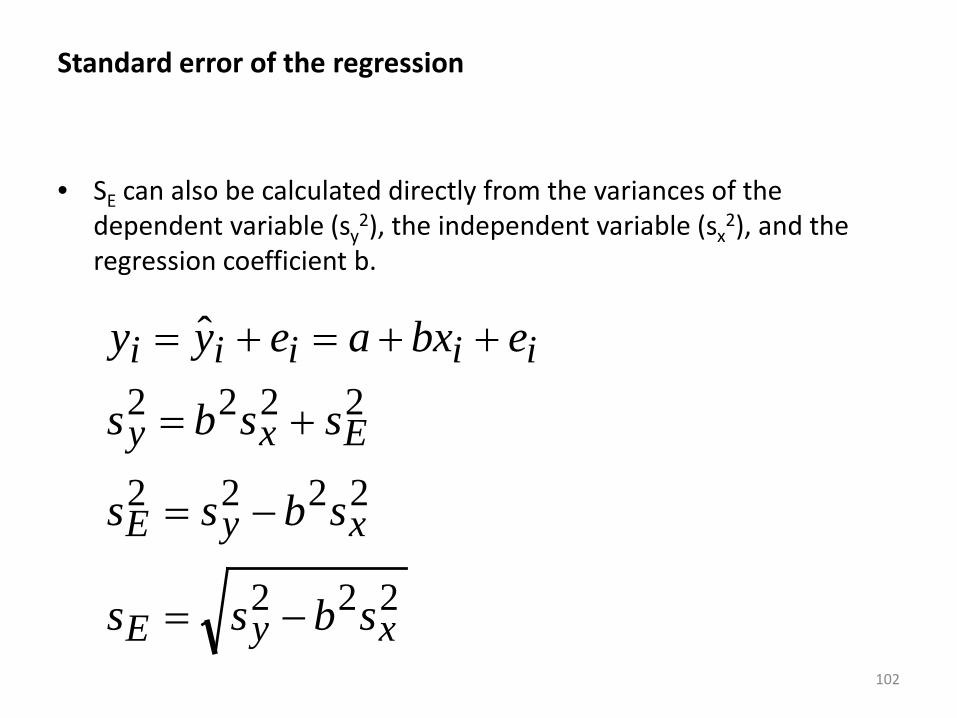
Standard error of the regression

• SE can also be calculated directly from the variances of the dependent variable (sy

2), the independent variable (sx2), and the

regression coefficient b.

222

2222

2222

ˆ

xyE

xyE

Exy

iiiii

sbss

sbss

ssbs

ebxaeyy

−=

−=

+=

++=+=

102

Standard error of the regression

• To turn this into an estimate of the population parameter, we need to correct it.

• STATA displays this value as the root MSE.

21222

−−

−=nnsbsS xyE

103

104


y' = 3.605 + (-0.124)x

r2

• Another measure of goodness-of-fit is the square of the correlation coefficient, r2.

• This measure is the proportional reduction in the variance of the residuals achieved by moving – From a model in which y is predicted solely by its mean – That is, a model with no explanatory variables, only an intercept term.

iii eyyyy +== so ˆ

– To a model in which y is predicted as a linear function of another variable

iiiii ebxaybxay ++=+= so ˆ105

• In the first model, the variance of the residuals will be equal to the variance of y.

• In the second model, the variance of the residuals will be equal to…

2222xyE sbss −=

• The proportional reduction in the variance of the residuals

going from the first to the second will be…

2

22

2

2222

21

22

212 )(

y

x

y

xyy

E

EE

ssb

ssbss

SSSr =

−−=

−=

106

• r2 can also be thought of as the proportional reduction in the residual sum of squares in going from a model in which y' is the average of y, to one in where it is a linear function: – Both of the following equations are the same, just using different notation

standards.

TSSTSSRSSTSSr SS Reg2 =

−=

SSTSSR

SSTSSESSTr =

−=2

107

108


y' = 3.605 + (-0.124)x

SOC 2010 Lecture 5

Documents