Actuarial Study Materials Learning Made Easier With Study Plus + SOA Exam LTAM Study Manual 1st Edition, Second Printing Abraham Weishaus, Ph.D., F.S.A., CFA, M.A.A.A. NO RETURN IF OPENED Study Plus + gives you digital access* to: • Flashcards • Actuarial Exam & Career Strategy Guides • Technical Skill eLearning Tools • Samples of Supplemental Textbook • And more! *See inside for keycode access and login instructions

Welcome message from author
This document is posted to help you gain knowledge. Please leave a comment to let me know what you think about it! Share it to your friends and learn new things together.
Transcript

Actuarial Study MaterialsLearning Made Easier
With StudyPlus+
SOA Exam LTAMStudy Manual
1st Edition, Second PrintingAbraham Weishaus, Ph.D., F.S.A., CFA, M.A.A.A.
NO RETURN IF OPENED
StudyPlus+ gives you digital access* to:• Flashcards
• Actuarial Exam & Career Strategy Guides
• Technical Skill eLearning Tools
• Samples of Supplemental Textbook
• And more!
*See inside for keycode access and login instructions

Contents
1 Probability Review 11.1 Functions and moments . . . . . . . . . . . . . . . . . . . . . . . . . . . . . . . . . . . . . . . . . 11.2 Probability distributions . . . . . . . . . . . . . . . . . . . . . . . . . . . . . . . . . . . . . . . . . 2
1.2.1 Bernoulli distribution . . . . . . . . . . . . . . . . . . . . . . . . . . . . . . . . . . . . . . 31.2.2 Uniform distribution . . . . . . . . . . . . . . . . . . . . . . . . . . . . . . . . . . . . . . . 31.2.3 Exponential distribution . . . . . . . . . . . . . . . . . . . . . . . . . . . . . . . . . . . . . 4
1.3 Variance . . . . . . . . . . . . . . . . . . . . . . . . . . . . . . . . . . . . . . . . . . . . . . . . . . 41.4 Normal approximation . . . . . . . . . . . . . . . . . . . . . . . . . . . . . . . . . . . . . . . . . . 51.5 Conditional probability and expectation . . . . . . . . . . . . . . . . . . . . . . . . . . . . . . . . 61.6 Conditional variance . . . . . . . . . . . . . . . . . . . . . . . . . . . . . . . . . . . . . . . . . . . 8
Exercises . . . . . . . . . . . . . . . . . . . . . . . . . . . . . . . . . . . . . . . . . . . . . . . . . . 9Solutions . . . . . . . . . . . . . . . . . . . . . . . . . . . . . . . . . . . . . . . . . . . . . . . . . . 13
2 Introduction to Long Term Insurance 19
I Survival Models 21
3 Survival Distributions: Probability Functions 233.1 Probability notation . . . . . . . . . . . . . . . . . . . . . . . . . . . . . . . . . . . . . . . . . . . . 233.2 Actuarial notation . . . . . . . . . . . . . . . . . . . . . . . . . . . . . . . . . . . . . . . . . . . . . 263.3 Life tables . . . . . . . . . . . . . . . . . . . . . . . . . . . . . . . . . . . . . . . . . . . . . . . . . 27
Exercises . . . . . . . . . . . . . . . . . . . . . . . . . . . . . . . . . . . . . . . . . . . . . . . . . . 29Solutions . . . . . . . . . . . . . . . . . . . . . . . . . . . . . . . . . . . . . . . . . . . . . . . . . . 35
4 Survival Distributions: Force of Mortality 41Exercises . . . . . . . . . . . . . . . . . . . . . . . . . . . . . . . . . . . . . . . . . . . . . . . . . . 46Solutions . . . . . . . . . . . . . . . . . . . . . . . . . . . . . . . . . . . . . . . . . . . . . . . . . . 54
5 Survival Distributions: Mortality Laws 655.1 Mortality laws that may be used for human mortality . . . . . . . . . . . . . . . . . . . . . . . . 65
5.1.1 Gompertz’s law . . . . . . . . . . . . . . . . . . . . . . . . . . . . . . . . . . . . . . . . . . 685.1.2 Makeham’s law . . . . . . . . . . . . . . . . . . . . . . . . . . . . . . . . . . . . . . . . . . 685.1.3 Weibull Distribution . . . . . . . . . . . . . . . . . . . . . . . . . . . . . . . . . . . . . . . 69
5.2 Mortality laws for easy computation . . . . . . . . . . . . . . . . . . . . . . . . . . . . . . . . . . 705.2.1 Exponential distribution, or constant force of mortality . . . . . . . . . . . . . . . . . . . 705.2.2 Uniform distribution . . . . . . . . . . . . . . . . . . . . . . . . . . . . . . . . . . . . . . . 705.2.3 Beta distribution . . . . . . . . . . . . . . . . . . . . . . . . . . . . . . . . . . . . . . . . . 71
5.3 British mortality tables . . . . . . . . . . . . . . . . . . . . . . . . . . . . . . . . . . . . . . . . . . 73Exercises . . . . . . . . . . . . . . . . . . . . . . . . . . . . . . . . . . . . . . . . . . . . . . . . . . 73Solutions . . . . . . . . . . . . . . . . . . . . . . . . . . . . . . . . . . . . . . . . . . . . . . . . . . 77
6 Survival Distributions: Moments 836.1 Complete . . . . . . . . . . . . . . . . . . . . . . . . . . . . . . . . . . . . . . . . . . . . . . . . . . 83
6.1.1 General . . . . . . . . . . . . . . . . . . . . . . . . . . . . . . . . . . . . . . . . . . . . . . . 836.1.2 Special mortality laws . . . . . . . . . . . . . . . . . . . . . . . . . . . . . . . . . . . . . . 85
6.2 Curtate . . . . . . . . . . . . . . . . . . . . . . . . . . . . . . . . . . . . . . . . . . . . . . . . . . . 88
SOA LTAM Study Manual—1st edition 2nd printingCopyright ©2018 ASM
iii

iv CONTENTS
Exercises . . . . . . . . . . . . . . . . . . . . . . . . . . . . . . . . . . . . . . . . . . . . . . . . . . 92Solutions . . . . . . . . . . . . . . . . . . . . . . . . . . . . . . . . . . . . . . . . . . . . . . . . . . 101
7 Survival Distributions: Percentiles and Recursions 1157.1 Percentiles . . . . . . . . . . . . . . . . . . . . . . . . . . . . . . . . . . . . . . . . . . . . . . . . . 1157.2 Recursive formulas for life expectancy . . . . . . . . . . . . . . . . . . . . . . . . . . . . . . . . . 116
Exercises . . . . . . . . . . . . . . . . . . . . . . . . . . . . . . . . . . . . . . . . . . . . . . . . . . 118Solutions . . . . . . . . . . . . . . . . . . . . . . . . . . . . . . . . . . . . . . . . . . . . . . . . . . 122
8 Survival Distributions: Fractional Ages 1298.1 Uniform distribution of deaths . . . . . . . . . . . . . . . . . . . . . . . . . . . . . . . . . . . . . 1298.2 Constant force of mortality . . . . . . . . . . . . . . . . . . . . . . . . . . . . . . . . . . . . . . . . 134
Exercises . . . . . . . . . . . . . . . . . . . . . . . . . . . . . . . . . . . . . . . . . . . . . . . . . . 135Solutions . . . . . . . . . . . . . . . . . . . . . . . . . . . . . . . . . . . . . . . . . . . . . . . . . . 142
9 Survival Distributions: Select Mortality 151Exercises . . . . . . . . . . . . . . . . . . . . . . . . . . . . . . . . . . . . . . . . . . . . . . . . . . 156Solutions . . . . . . . . . . . . . . . . . . . . . . . . . . . . . . . . . . . . . . . . . . . . . . . . . . 164
10 Survival Distributions: Models for Mortality Improvement 17710.1 Deterministic mortality improvement models . . . . . . . . . . . . . . . . . . . . . . . . . . . . . 17710.2 Stochastic mortality improvement models . . . . . . . . . . . . . . . . . . . . . . . . . . . . . . . 180
10.2.1 The Lee Carter model . . . . . . . . . . . . . . . . . . . . . . . . . . . . . . . . . . . . . . 18210.2.2 The Cairns-Blake-Dowd (CBD) models . . . . . . . . . . . . . . . . . . . . . . . . . . . . 186Exercises . . . . . . . . . . . . . . . . . . . . . . . . . . . . . . . . . . . . . . . . . . . . . . . . . . 189Solutions . . . . . . . . . . . . . . . . . . . . . . . . . . . . . . . . . . . . . . . . . . . . . . . . . . 195
11 Supplementary Questions: Survival Distributions 201Solutions . . . . . . . . . . . . . . . . . . . . . . . . . . . . . . . . . . . . . . . . . . . . . . . . . . 203
II Insurances 209
12 Insurance: Annual and 1/mthly—Moments 21112.1 Review of Financial Mathematics . . . . . . . . . . . . . . . . . . . . . . . . . . . . . . . . . . . . 21112.2 Moments of annual insurances . . . . . . . . . . . . . . . . . . . . . . . . . . . . . . . . . . . . . 21212.3 Standard insurances and notation . . . . . . . . . . . . . . . . . . . . . . . . . . . . . . . . . . . . 21312.4 Standard Ultimate Life Table . . . . . . . . . . . . . . . . . . . . . . . . . . . . . . . . . . . . . . . 21512.5 Constant force and uniform mortality . . . . . . . . . . . . . . . . . . . . . . . . . . . . . . . . . 21712.6 Normal approximation . . . . . . . . . . . . . . . . . . . . . . . . . . . . . . . . . . . . . . . . . . 21912.7 1/mthly insurance . . . . . . . . . . . . . . . . . . . . . . . . . . . . . . . . . . . . . . . . . . . . . 220
Exercises . . . . . . . . . . . . . . . . . . . . . . . . . . . . . . . . . . . . . . . . . . . . . . . . . . 221Solutions . . . . . . . . . . . . . . . . . . . . . . . . . . . . . . . . . . . . . . . . . . . . . . . . . . 236
13 Insurance: Continuous—Moments—Part 1 24913.1 Definitions and general formulas . . . . . . . . . . . . . . . . . . . . . . . . . . . . . . . . . . . . 24913.2 Constant force of mortality . . . . . . . . . . . . . . . . . . . . . . . . . . . . . . . . . . . . . . . . 250
Exercises . . . . . . . . . . . . . . . . . . . . . . . . . . . . . . . . . . . . . . . . . . . . . . . . . . 257Solutions . . . . . . . . . . . . . . . . . . . . . . . . . . . . . . . . . . . . . . . . . . . . . . . . . . 267
14 Insurance: Continuous—Moments—Part 2 27714.1 Uniform survival function . . . . . . . . . . . . . . . . . . . . . . . . . . . . . . . . . . . . . . . . 27714.2 Other mortality functions . . . . . . . . . . . . . . . . . . . . . . . . . . . . . . . . . . . . . . . . 279
SOA LTAM Study Manual—1st edition 2nd printingCopyright ©2018 ASM
CONTENTS v
14.2.1 Integrating atn e−ct (Gamma Integrands) . . . . . . . . . . . . . . . . . . . . . . . . . . . 27914.3 Variance of endowment insurance . . . . . . . . . . . . . . . . . . . . . . . . . . . . . . . . . . . 28014.4 Normal approximation . . . . . . . . . . . . . . . . . . . . . . . . . . . . . . . . . . . . . . . . . . 282
Exercises . . . . . . . . . . . . . . . . . . . . . . . . . . . . . . . . . . . . . . . . . . . . . . . . . . 283Solutions . . . . . . . . . . . . . . . . . . . . . . . . . . . . . . . . . . . . . . . . . . . . . . . . . . 290
15 Insurance: Probabilities and Percentiles 29915.1 Introduction . . . . . . . . . . . . . . . . . . . . . . . . . . . . . . . . . . . . . . . . . . . . . . . . 29915.2 Probabilities for continuous insurance variables . . . . . . . . . . . . . . . . . . . . . . . . . . . 30015.3 Distribution functions of insurance present values . . . . . . . . . . . . . . . . . . . . . . . . . . 30415.4 Probabilities for discrete variables . . . . . . . . . . . . . . . . . . . . . . . . . . . . . . . . . . . 30515.5 Percentiles . . . . . . . . . . . . . . . . . . . . . . . . . . . . . . . . . . . . . . . . . . . . . . . . . 306
Exercises . . . . . . . . . . . . . . . . . . . . . . . . . . . . . . . . . . . . . . . . . . . . . . . . . . 309Solutions . . . . . . . . . . . . . . . . . . . . . . . . . . . . . . . . . . . . . . . . . . . . . . . . . . 313
16 Insurance: Recursive Formulas, Varying Insurance 32316.1 Recursive formulas . . . . . . . . . . . . . . . . . . . . . . . . . . . . . . . . . . . . . . . . . . . . 32316.2 Varying insurance . . . . . . . . . . . . . . . . . . . . . . . . . . . . . . . . . . . . . . . . . . . . . 325
Exercises . . . . . . . . . . . . . . . . . . . . . . . . . . . . . . . . . . . . . . . . . . . . . . . . . . 333Solutions . . . . . . . . . . . . . . . . . . . . . . . . . . . . . . . . . . . . . . . . . . . . . . . . . . 341
17 Insurance: Relationships between Ax , A(m)x , and Ax 35317.1 Uniform distribution of deaths . . . . . . . . . . . . . . . . . . . . . . . . . . . . . . . . . . . . . 35317.2 Claims acceleration approach . . . . . . . . . . . . . . . . . . . . . . . . . . . . . . . . . . . . . . 355
Exercises . . . . . . . . . . . . . . . . . . . . . . . . . . . . . . . . . . . . . . . . . . . . . . . . . . 356Solutions . . . . . . . . . . . . . . . . . . . . . . . . . . . . . . . . . . . . . . . . . . . . . . . . . . 359
18 Supplementary Questions: Insurances 363Solutions . . . . . . . . . . . . . . . . . . . . . . . . . . . . . . . . . . . . . . . . . . . . . . . . . . 364
III Annuities 367
19 Annuities: Discrete, Expectation 36919.1 Annuities-due . . . . . . . . . . . . . . . . . . . . . . . . . . . . . . . . . . . . . . . . . . . . . . . 36919.2 Annuities-immediate . . . . . . . . . . . . . . . . . . . . . . . . . . . . . . . . . . . . . . . . . . . 37419.3 1/mthly annuities . . . . . . . . . . . . . . . . . . . . . . . . . . . . . . . . . . . . . . . . . . . . . 37719.4 Actuarial Accumulated Value . . . . . . . . . . . . . . . . . . . . . . . . . . . . . . . . . . . . . . 378
Exercises . . . . . . . . . . . . . . . . . . . . . . . . . . . . . . . . . . . . . . . . . . . . . . . . . . 380Solutions . . . . . . . . . . . . . . . . . . . . . . . . . . . . . . . . . . . . . . . . . . . . . . . . . . 391
20 Annuities: Continuous, Expectation 40320.1 Whole life annuity . . . . . . . . . . . . . . . . . . . . . . . . . . . . . . . . . . . . . . . . . . . . 40320.2 Temporary and deferred life annuities . . . . . . . . . . . . . . . . . . . . . . . . . . . . . . . . . 40620.3 n-year certain-and-life annuity . . . . . . . . . . . . . . . . . . . . . . . . . . . . . . . . . . . . . 409
Exercises . . . . . . . . . . . . . . . . . . . . . . . . . . . . . . . . . . . . . . . . . . . . . . . . . . 411Solutions . . . . . . . . . . . . . . . . . . . . . . . . . . . . . . . . . . . . . . . . . . . . . . . . . . 417
21 Annuities: Variance 42521.1 Whole Life and Temporary Life Annuities . . . . . . . . . . . . . . . . . . . . . . . . . . . . . . . 42521.2 Other Annuities . . . . . . . . . . . . . . . . . . . . . . . . . . . . . . . . . . . . . . . . . . . . . . 42721.3 Typical Exam Questions . . . . . . . . . . . . . . . . . . . . . . . . . . . . . . . . . . . . . . . . . 427
SOA LTAM Study Manual—1st edition 2nd printingCopyright ©2018 ASM
vi CONTENTS
21.4 Combinations of Annuities and Insurances with No Variance . . . . . . . . . . . . . . . . . . . . 430Exercises . . . . . . . . . . . . . . . . . . . . . . . . . . . . . . . . . . . . . . . . . . . . . . . . . . 431Solutions . . . . . . . . . . . . . . . . . . . . . . . . . . . . . . . . . . . . . . . . . . . . . . . . . . 441
22 Annuities: Probabilities and Percentiles 45522.1 Probabilities for continuous annuities . . . . . . . . . . . . . . . . . . . . . . . . . . . . . . . . . 45522.2 Distribution functions of annuity present values . . . . . . . . . . . . . . . . . . . . . . . . . . . 45722.3 Probabilities for discrete annuities . . . . . . . . . . . . . . . . . . . . . . . . . . . . . . . . . . . 45822.4 Percentiles . . . . . . . . . . . . . . . . . . . . . . . . . . . . . . . . . . . . . . . . . . . . . . . . . 460
Exercises . . . . . . . . . . . . . . . . . . . . . . . . . . . . . . . . . . . . . . . . . . . . . . . . . . 463Solutions . . . . . . . . . . . . . . . . . . . . . . . . . . . . . . . . . . . . . . . . . . . . . . . . . . 467
23 Annuities: Varying Annuities, Recursive Formulas 47523.1 Increasing and Decreasing Annuities . . . . . . . . . . . . . . . . . . . . . . . . . . . . . . . . . . 475
23.1.1 Geometrically increasing annuities . . . . . . . . . . . . . . . . . . . . . . . . . . . . . . . 47523.1.2 Arithmetically increasing annuities . . . . . . . . . . . . . . . . . . . . . . . . . . . . . . 475
23.2 Recursive formulas . . . . . . . . . . . . . . . . . . . . . . . . . . . . . . . . . . . . . . . . . . . . 477Exercises . . . . . . . . . . . . . . . . . . . . . . . . . . . . . . . . . . . . . . . . . . . . . . . . . . 478Solutions . . . . . . . . . . . . . . . . . . . . . . . . . . . . . . . . . . . . . . . . . . . . . . . . . . 484
24 Annuities: 1/m-thly Payments 49124.1 Uniform distribution of deaths assumption . . . . . . . . . . . . . . . . . . . . . . . . . . . . . . 49124.2 Woolhouse’s formula . . . . . . . . . . . . . . . . . . . . . . . . . . . . . . . . . . . . . . . . . . . 492
Exercises . . . . . . . . . . . . . . . . . . . . . . . . . . . . . . . . . . . . . . . . . . . . . . . . . . 496Solutions . . . . . . . . . . . . . . . . . . . . . . . . . . . . . . . . . . . . . . . . . . . . . . . . . . 500
25 Supplementary Questions: Annuities 507Solutions . . . . . . . . . . . . . . . . . . . . . . . . . . . . . . . . . . . . . . . . . . . . . . . . . . 510
IV Premiums 515
26 Premiums: Net Premiums for Discrete Insurances—Part 1 51726.1 Future loss . . . . . . . . . . . . . . . . . . . . . . . . . . . . . . . . . . . . . . . . . . . . . . . . . 51726.2 Net premium . . . . . . . . . . . . . . . . . . . . . . . . . . . . . . . . . . . . . . . . . . . . . . . 518
Exercises . . . . . . . . . . . . . . . . . . . . . . . . . . . . . . . . . . . . . . . . . . . . . . . . . . 520Solutions . . . . . . . . . . . . . . . . . . . . . . . . . . . . . . . . . . . . . . . . . . . . . . . . . . 529
27 Premiums: Net Premiums for Discrete Insurances—Part 2 53927.1 Premium formulas . . . . . . . . . . . . . . . . . . . . . . . . . . . . . . . . . . . . . . . . . . . . 53927.2 Expected value of future loss . . . . . . . . . . . . . . . . . . . . . . . . . . . . . . . . . . . . . . 54127.3 International Actuarial Premium Notation . . . . . . . . . . . . . . . . . . . . . . . . . . . . . . . 542
Exercises . . . . . . . . . . . . . . . . . . . . . . . . . . . . . . . . . . . . . . . . . . . . . . . . . . 544Solutions . . . . . . . . . . . . . . . . . . . . . . . . . . . . . . . . . . . . . . . . . . . . . . . . . . 551
28 Premiums: Net Premiums Paid on a 1/mthly Basis 561Exercises . . . . . . . . . . . . . . . . . . . . . . . . . . . . . . . . . . . . . . . . . . . . . . . . . . 562Solutions . . . . . . . . . . . . . . . . . . . . . . . . . . . . . . . . . . . . . . . . . . . . . . . . . . 566
29 Premiums: Net Premiums for Fully Continuous Insurances 571Exercises . . . . . . . . . . . . . . . . . . . . . . . . . . . . . . . . . . . . . . . . . . . . . . . . . . 574Solutions . . . . . . . . . . . . . . . . . . . . . . . . . . . . . . . . . . . . . . . . . . . . . . . . . . 580
SOA LTAM Study Manual—1st edition 2nd printingCopyright ©2018 ASM

CONTENTS vii
30 Premiums: Gross Premiums 58730.1 Gross future loss . . . . . . . . . . . . . . . . . . . . . . . . . . . . . . . . . . . . . . . . . . . . . 58730.2 Gross premium . . . . . . . . . . . . . . . . . . . . . . . . . . . . . . . . . . . . . . . . . . . . . . 588
Exercises . . . . . . . . . . . . . . . . . . . . . . . . . . . . . . . . . . . . . . . . . . . . . . . . . . 590Solutions . . . . . . . . . . . . . . . . . . . . . . . . . . . . . . . . . . . . . . . . . . . . . . . . . . 597
31 Premiums: Variance of Future Loss, Discrete 60331.1 Variance of net future loss . . . . . . . . . . . . . . . . . . . . . . . . . . . . . . . . . . . . . . . . 603
31.1.1 Variance of net future loss by formula . . . . . . . . . . . . . . . . . . . . . . . . . . . . . 60331.1.2 Variance of net future loss from first principles . . . . . . . . . . . . . . . . . . . . . . . . 605
31.2 Variance of gross future loss . . . . . . . . . . . . . . . . . . . . . . . . . . . . . . . . . . . . . . . 606Exercises . . . . . . . . . . . . . . . . . . . . . . . . . . . . . . . . . . . . . . . . . . . . . . . . . . 608Solutions . . . . . . . . . . . . . . . . . . . . . . . . . . . . . . . . . . . . . . . . . . . . . . . . . . 614
32 Premiums: Variance of Future Loss, Continuous 62332.1 Variance of net future loss . . . . . . . . . . . . . . . . . . . . . . . . . . . . . . . . . . . . . . . . 62332.2 Variance of gross future loss . . . . . . . . . . . . . . . . . . . . . . . . . . . . . . . . . . . . . . . 624
Exercises . . . . . . . . . . . . . . . . . . . . . . . . . . . . . . . . . . . . . . . . . . . . . . . . . . 625Solutions . . . . . . . . . . . . . . . . . . . . . . . . . . . . . . . . . . . . . . . . . . . . . . . . . . 632
33 Premiums: Probabilities and Percentiles of Future Loss 64133.1 Probabilities . . . . . . . . . . . . . . . . . . . . . . . . . . . . . . . . . . . . . . . . . . . . . . . . 641
33.1.1 Fully continuous insurances . . . . . . . . . . . . . . . . . . . . . . . . . . . . . . . . . . . 64133.1.2 Discrete insurances . . . . . . . . . . . . . . . . . . . . . . . . . . . . . . . . . . . . . . . . 64533.1.3 Annuities . . . . . . . . . . . . . . . . . . . . . . . . . . . . . . . . . . . . . . . . . . . . . 64533.1.4 Gross future loss . . . . . . . . . . . . . . . . . . . . . . . . . . . . . . . . . . . . . . . . . 648
33.2 Percentiles . . . . . . . . . . . . . . . . . . . . . . . . . . . . . . . . . . . . . . . . . . . . . . . . . 649Exercises . . . . . . . . . . . . . . . . . . . . . . . . . . . . . . . . . . . . . . . . . . . . . . . . . . 650Solutions . . . . . . . . . . . . . . . . . . . . . . . . . . . . . . . . . . . . . . . . . . . . . . . . . . 653
34 Premiums: Special Topics 66134.1 The portfolio percentile premium principle . . . . . . . . . . . . . . . . . . . . . . . . . . . . . . 66134.2 Extra risks . . . . . . . . . . . . . . . . . . . . . . . . . . . . . . . . . . . . . . . . . . . . . . . . . 663
Exercises . . . . . . . . . . . . . . . . . . . . . . . . . . . . . . . . . . . . . . . . . . . . . . . . . . 663Solutions . . . . . . . . . . . . . . . . . . . . . . . . . . . . . . . . . . . . . . . . . . . . . . . . . . 665
35 Supplementary Questions: Premiums 669Solutions . . . . . . . . . . . . . . . . . . . . . . . . . . . . . . . . . . . . . . . . . . . . . . . . . . 672
V Reserves 679
36 Reserves: Net Premium Reserve 681Exercises . . . . . . . . . . . . . . . . . . . . . . . . . . . . . . . . . . . . . . . . . . . . . . . . . . 686Solutions . . . . . . . . . . . . . . . . . . . . . . . . . . . . . . . . . . . . . . . . . . . . . . . . . . 693
37 Reserves: Gross Premium Reserve and Expense Reserve 70337.1 Gross premium reserve . . . . . . . . . . . . . . . . . . . . . . . . . . . . . . . . . . . . . . . . . . 70337.2 Expense reserve . . . . . . . . . . . . . . . . . . . . . . . . . . . . . . . . . . . . . . . . . . . . . . 705
Exercises . . . . . . . . . . . . . . . . . . . . . . . . . . . . . . . . . . . . . . . . . . . . . . . . . . 707Solutions . . . . . . . . . . . . . . . . . . . . . . . . . . . . . . . . . . . . . . . . . . . . . . . . . . 710
SOA LTAM Study Manual—1st edition 2nd printingCopyright ©2018 ASM
viii CONTENTS
38 Reserves: Special Formulas for Whole Life and Endowment Insurance 71538.1 Annuity-ratio formula . . . . . . . . . . . . . . . . . . . . . . . . . . . . . . . . . . . . . . . . . . 71538.2 Insurance-ratio formula . . . . . . . . . . . . . . . . . . . . . . . . . . . . . . . . . . . . . . . . . 71638.3 Premium-ratio formula . . . . . . . . . . . . . . . . . . . . . . . . . . . . . . . . . . . . . . . . . . 717
Exercises . . . . . . . . . . . . . . . . . . . . . . . . . . . . . . . . . . . . . . . . . . . . . . . . . . 719Solutions . . . . . . . . . . . . . . . . . . . . . . . . . . . . . . . . . . . . . . . . . . . . . . . . . . 727
39 Reserves: Variance of Loss 737Exercises . . . . . . . . . . . . . . . . . . . . . . . . . . . . . . . . . . . . . . . . . . . . . . . . . . 739Solutions . . . . . . . . . . . . . . . . . . . . . . . . . . . . . . . . . . . . . . . . . . . . . . . . . . 745
40 Reserves: Recursive Formulas 75340.1 Net premium reserve . . . . . . . . . . . . . . . . . . . . . . . . . . . . . . . . . . . . . . . . . . . 75340.2 Insurances and annuities with payment of reserve upon death . . . . . . . . . . . . . . . . . . . 75640.3 Gross premium reserve . . . . . . . . . . . . . . . . . . . . . . . . . . . . . . . . . . . . . . . . . . 760
Exercises . . . . . . . . . . . . . . . . . . . . . . . . . . . . . . . . . . . . . . . . . . . . . . . . . . 763Solutions . . . . . . . . . . . . . . . . . . . . . . . . . . . . . . . . . . . . . . . . . . . . . . . . . . 782
41 Reserves: Modified Reserves 801Exercises . . . . . . . . . . . . . . . . . . . . . . . . . . . . . . . . . . . . . . . . . . . . . . . . . . 802Solutions . . . . . . . . . . . . . . . . . . . . . . . . . . . . . . . . . . . . . . . . . . . . . . . . . . 806
42 Reserves: Other Topics 81342.1 Reserves on semicontinuous insurance . . . . . . . . . . . . . . . . . . . . . . . . . . . . . . . . . 81342.2 Reserves between premium dates . . . . . . . . . . . . . . . . . . . . . . . . . . . . . . . . . . . . 81442.3 Thiele’s differential equation . . . . . . . . . . . . . . . . . . . . . . . . . . . . . . . . . . . . . . . 816
Exercises . . . . . . . . . . . . . . . . . . . . . . . . . . . . . . . . . . . . . . . . . . . . . . . . . . 820Solutions . . . . . . . . . . . . . . . . . . . . . . . . . . . . . . . . . . . . . . . . . . . . . . . . . . 827
43 Supplementary Questions: Reserves 837Solutions . . . . . . . . . . . . . . . . . . . . . . . . . . . . . . . . . . . . . . . . . . . . . . . . . . 839
VI Markov Chains 845
44 Markov Chains: Discrete—Probabilities 84744.1 Introduction . . . . . . . . . . . . . . . . . . . . . . . . . . . . . . . . . . . . . . . . . . . . . . . . 84744.2 Definition of Markov chains . . . . . . . . . . . . . . . . . . . . . . . . . . . . . . . . . . . . . . . 85044.3 Discrete Markov chains . . . . . . . . . . . . . . . . . . . . . . . . . . . . . . . . . . . . . . . . . . 851
Exercises . . . . . . . . . . . . . . . . . . . . . . . . . . . . . . . . . . . . . . . . . . . . . . . . . . 854Solutions . . . . . . . . . . . . . . . . . . . . . . . . . . . . . . . . . . . . . . . . . . . . . . . . . . 857
45 Markov Chains: Continuous—Probabilities 86145.1 Probabilities—direct calculation . . . . . . . . . . . . . . . . . . . . . . . . . . . . . . . . . . . . . 86245.2 Kolmogorov’s forward equations . . . . . . . . . . . . . . . . . . . . . . . . . . . . . . . . . . . . 865
Exercises . . . . . . . . . . . . . . . . . . . . . . . . . . . . . . . . . . . . . . . . . . . . . . . . . . 867Solutions . . . . . . . . . . . . . . . . . . . . . . . . . . . . . . . . . . . . . . . . . . . . . . . . . . 876
46 Markov Chains: Premiums and Reserves 88346.1 Premiums . . . . . . . . . . . . . . . . . . . . . . . . . . . . . . . . . . . . . . . . . . . . . . . . . 88346.2 Reserves . . . . . . . . . . . . . . . . . . . . . . . . . . . . . . . . . . . . . . . . . . . . . . . . . . 88746.3 Reserve recursions . . . . . . . . . . . . . . . . . . . . . . . . . . . . . . . . . . . . . . . . . . . . 889
SOA LTAM Study Manual—1st edition 2nd printingCopyright ©2018 ASM

CONTENTS ix
Exercises . . . . . . . . . . . . . . . . . . . . . . . . . . . . . . . . . . . . . . . . . . . . . . . . . . 892Solutions . . . . . . . . . . . . . . . . . . . . . . . . . . . . . . . . . . . . . . . . . . . . . . . . . . 903
47 Applications of Markov Chains 91347.1 Disability income insurance . . . . . . . . . . . . . . . . . . . . . . . . . . . . . . . . . . . . . . . 913
47.1.1 Features of disability income insurance . . . . . . . . . . . . . . . . . . . . . . . . . . . . 91347.1.2 Premiums and reserves for disability income insurance . . . . . . . . . . . . . . . . . . . 914
47.2 Hospital indemnity insurance . . . . . . . . . . . . . . . . . . . . . . . . . . . . . . . . . . . . . . 91547.3 Long Term Care Insurance (LTC) . . . . . . . . . . . . . . . . . . . . . . . . . . . . . . . . . . . . 915
47.3.1 Features of LTC . . . . . . . . . . . . . . . . . . . . . . . . . . . . . . . . . . . . . . . . . . 91547.3.2 Models for LTC . . . . . . . . . . . . . . . . . . . . . . . . . . . . . . . . . . . . . . . . . . 917
47.4 Critical Illness and Chronic Illness Insurance . . . . . . . . . . . . . . . . . . . . . . . . . . . . . 92047.5 Continuing care retirement communities (CCRCs) . . . . . . . . . . . . . . . . . . . . . . . . . . 921
47.5.1 Features of CCRCs . . . . . . . . . . . . . . . . . . . . . . . . . . . . . . . . . . . . . . . . 92147.5.2 Models for CCRCs . . . . . . . . . . . . . . . . . . . . . . . . . . . . . . . . . . . . . . . . 922
47.6 Structured settlements . . . . . . . . . . . . . . . . . . . . . . . . . . . . . . . . . . . . . . . . . . 924Exercises . . . . . . . . . . . . . . . . . . . . . . . . . . . . . . . . . . . . . . . . . . . . . . . . . . 927Solutions . . . . . . . . . . . . . . . . . . . . . . . . . . . . . . . . . . . . . . . . . . . . . . . . . . 939
VII Multiple Decrements 947
48 Multiple Decrement Models: Probabilities 94948.1 Probabilities . . . . . . . . . . . . . . . . . . . . . . . . . . . . . . . . . . . . . . . . . . . . . . . . 94948.2 Life tables . . . . . . . . . . . . . . . . . . . . . . . . . . . . . . . . . . . . . . . . . . . . . . . . . 95148.3 Examples of Multiple Decrement Probabilities . . . . . . . . . . . . . . . . . . . . . . . . . . . . 95248.4 Discrete Insurances . . . . . . . . . . . . . . . . . . . . . . . . . . . . . . . . . . . . . . . . . . . . 953
Exercises . . . . . . . . . . . . . . . . . . . . . . . . . . . . . . . . . . . . . . . . . . . . . . . . . . 954Solutions . . . . . . . . . . . . . . . . . . . . . . . . . . . . . . . . . . . . . . . . . . . . . . . . . . 967
49 Multiple Decrement Models: Forces of Decrement 97549.1 µ
( j)x . . . . . . . . . . . . . . . . . . . . . . . . . . . . . . . . . . . . . . . . . . . . . . . . . . . . . 975
49.2 Probability framework for multiple decrement models . . . . . . . . . . . . . . . . . . . . . . . . 97749.3 Fractional ages . . . . . . . . . . . . . . . . . . . . . . . . . . . . . . . . . . . . . . . . . . . . . . . 979
Exercises . . . . . . . . . . . . . . . . . . . . . . . . . . . . . . . . . . . . . . . . . . . . . . . . . . 979Solutions . . . . . . . . . . . . . . . . . . . . . . . . . . . . . . . . . . . . . . . . . . . . . . . . . . 988
50 Multiple Decrement Models: Associated Single Decrement Tables 999Exercises . . . . . . . . . . . . . . . . . . . . . . . . . . . . . . . . . . . . . . . . . . . . . . . . . . 1003Solutions . . . . . . . . . . . . . . . . . . . . . . . . . . . . . . . . . . . . . . . . . . . . . . . . . . 1008
51 Multiple Decrement Models: Relations Between Rates 101751.1 Constant force of decrement . . . . . . . . . . . . . . . . . . . . . . . . . . . . . . . . . . . . . . . 101751.2 Uniform in the multiple-decrement tables . . . . . . . . . . . . . . . . . . . . . . . . . . . . . . . 101751.3 Uniform in the associated single-decrement tables . . . . . . . . . . . . . . . . . . . . . . . . . . 1020
Exercises . . . . . . . . . . . . . . . . . . . . . . . . . . . . . . . . . . . . . . . . . . . . . . . . . . 1024Solutions . . . . . . . . . . . . . . . . . . . . . . . . . . . . . . . . . . . . . . . . . . . . . . . . . . 1027
52 Multiple Decrement Models: Discrete Decrements 1035Exercises . . . . . . . . . . . . . . . . . . . . . . . . . . . . . . . . . . . . . . . . . . . . . . . . . . 1038Solutions . . . . . . . . . . . . . . . . . . . . . . . . . . . . . . . . . . . . . . . . . . . . . . . . . . 1043
SOA LTAM Study Manual—1st edition 2nd printingCopyright ©2018 ASM

x CONTENTS
53 Multiple Decrement Models: Continuous Insurances 1049Exercises . . . . . . . . . . . . . . . . . . . . . . . . . . . . . . . . . . . . . . . . . . . . . . . . . . 1052Solutions . . . . . . . . . . . . . . . . . . . . . . . . . . . . . . . . . . . . . . . . . . . . . . . . . . 1063
54 Supplementary Questions: Multiple Decrements 1077Solutions . . . . . . . . . . . . . . . . . . . . . . . . . . . . . . . . . . . . . . . . . . . . . . . . . . 1078
VIII Multiple Lives 1081
55 Multiple Lives: Joint Life Probabilities 108355.1 Markov chain model . . . . . . . . . . . . . . . . . . . . . . . . . . . . . . . . . . . . . . . . . . . 108355.2 Independent lives . . . . . . . . . . . . . . . . . . . . . . . . . . . . . . . . . . . . . . . . . . . . . 108455.3 Joint distribution function model . . . . . . . . . . . . . . . . . . . . . . . . . . . . . . . . . . . . 1086
Exercises . . . . . . . . . . . . . . . . . . . . . . . . . . . . . . . . . . . . . . . . . . . . . . . . . . 1088Solutions . . . . . . . . . . . . . . . . . . . . . . . . . . . . . . . . . . . . . . . . . . . . . . . . . . 1094
56 Multiple Lives: Last Survivor Probabilities 1099Exercises . . . . . . . . . . . . . . . . . . . . . . . . . . . . . . . . . . . . . . . . . . . . . . . . . . 1104Solutions . . . . . . . . . . . . . . . . . . . . . . . . . . . . . . . . . . . . . . . . . . . . . . . . . . 1110
57 Multiple Lives: Moments 1117Exercises . . . . . . . . . . . . . . . . . . . . . . . . . . . . . . . . . . . . . . . . . . . . . . . . . . 1122Solutions . . . . . . . . . . . . . . . . . . . . . . . . . . . . . . . . . . . . . . . . . . . . . . . . . . 1126
58 Multiple Lives: Contingent Probabilities 1133Exercises . . . . . . . . . . . . . . . . . . . . . . . . . . . . . . . . . . . . . . . . . . . . . . . . . . 1139Solutions . . . . . . . . . . . . . . . . . . . . . . . . . . . . . . . . . . . . . . . . . . . . . . . . . . 1145
59 Multiple Lives: Common Shock 1155Exercises . . . . . . . . . . . . . . . . . . . . . . . . . . . . . . . . . . . . . . . . . . . . . . . . . . 1157Solutions . . . . . . . . . . . . . . . . . . . . . . . . . . . . . . . . . . . . . . . . . . . . . . . . . . 1159
60 Multiple Lives: Insurances 116160.1 Joint and last survivor insurances . . . . . . . . . . . . . . . . . . . . . . . . . . . . . . . . . . . . 116160.2 Contingent insurances . . . . . . . . . . . . . . . . . . . . . . . . . . . . . . . . . . . . . . . . . . 116660.3 Common shock insurances . . . . . . . . . . . . . . . . . . . . . . . . . . . . . . . . . . . . . . . . 1168
Exercises . . . . . . . . . . . . . . . . . . . . . . . . . . . . . . . . . . . . . . . . . . . . . . . . . . 1169Solutions . . . . . . . . . . . . . . . . . . . . . . . . . . . . . . . . . . . . . . . . . . . . . . . . . . 1185
61 Multiple Lives: Annuities 120161.1 Introduction . . . . . . . . . . . . . . . . . . . . . . . . . . . . . . . . . . . . . . . . . . . . . . . . 120161.2 Three techniques for handling annuities . . . . . . . . . . . . . . . . . . . . . . . . . . . . . . . . 120261.3 Variance . . . . . . . . . . . . . . . . . . . . . . . . . . . . . . . . . . . . . . . . . . . . . . . . . . 1205
Exercises . . . . . . . . . . . . . . . . . . . . . . . . . . . . . . . . . . . . . . . . . . . . . . . . . . 1206Solutions . . . . . . . . . . . . . . . . . . . . . . . . . . . . . . . . . . . . . . . . . . . . . . . . . . 1216
62 Supplementary Questions: Multiple Lives 1227Solutions . . . . . . . . . . . . . . . . . . . . . . . . . . . . . . . . . . . . . . . . . . . . . . . . . . 1229
SOA LTAM Study Manual—1st edition 2nd printingCopyright ©2018 ASM

CONTENTS xi
IX Estimating Mortality Rates 1235
63 Review of Mathematical Statistics 123763.1 Estimator quality . . . . . . . . . . . . . . . . . . . . . . . . . . . . . . . . . . . . . . . . . . . . . 1237
63.1.1 Bias . . . . . . . . . . . . . . . . . . . . . . . . . . . . . . . . . . . . . . . . . . . . . . . . . 123863.1.2 Consistency . . . . . . . . . . . . . . . . . . . . . . . . . . . . . . . . . . . . . . . . . . . . 123963.1.3 Variance and mean square error . . . . . . . . . . . . . . . . . . . . . . . . . . . . . . . . 1240
63.2 Confidence intervals . . . . . . . . . . . . . . . . . . . . . . . . . . . . . . . . . . . . . . . . . . . 1241Exercises . . . . . . . . . . . . . . . . . . . . . . . . . . . . . . . . . . . . . . . . . . . . . . . . . . 1243Solutions . . . . . . . . . . . . . . . . . . . . . . . . . . . . . . . . . . . . . . . . . . . . . . . . . . 1247
64 The Empirical Distribution for Complete Data 125364.1 Individual data . . . . . . . . . . . . . . . . . . . . . . . . . . . . . . . . . . . . . . . . . . . . . . 125364.2 Grouped data . . . . . . . . . . . . . . . . . . . . . . . . . . . . . . . . . . . . . . . . . . . . . . . 1254
Exercises . . . . . . . . . . . . . . . . . . . . . . . . . . . . . . . . . . . . . . . . . . . . . . . . . . 1256Solutions . . . . . . . . . . . . . . . . . . . . . . . . . . . . . . . . . . . . . . . . . . . . . . . . . . 1259
65 Maximum Likelihood Estimators 126365.1 Defining the likelihood . . . . . . . . . . . . . . . . . . . . . . . . . . . . . . . . . . . . . . . . . . 1264
65.1.1 Individual data . . . . . . . . . . . . . . . . . . . . . . . . . . . . . . . . . . . . . . . . . . 126565.1.2 Grouped data . . . . . . . . . . . . . . . . . . . . . . . . . . . . . . . . . . . . . . . . . . . 126665.1.3 Censoring . . . . . . . . . . . . . . . . . . . . . . . . . . . . . . . . . . . . . . . . . . . . . 126665.1.4 Truncation . . . . . . . . . . . . . . . . . . . . . . . . . . . . . . . . . . . . . . . . . . . . . 126765.1.5 Combination of censoring and truncation . . . . . . . . . . . . . . . . . . . . . . . . . . . 1268Exercises . . . . . . . . . . . . . . . . . . . . . . . . . . . . . . . . . . . . . . . . . . . . . . . . . . 1268Solutions . . . . . . . . . . . . . . . . . . . . . . . . . . . . . . . . . . . . . . . . . . . . . . . . . . 1276
66 Kaplan-Meier and Nelson-Åalen Estimators 128366.1 Kaplan-Meier Estimator . . . . . . . . . . . . . . . . . . . . . . . . . . . . . . . . . . . . . . . . . 128466.2 Nelson-Åalen Estimator . . . . . . . . . . . . . . . . . . . . . . . . . . . . . . . . . . . . . . . . . 1288
Exercises . . . . . . . . . . . . . . . . . . . . . . . . . . . . . . . . . . . . . . . . . . . . . . . . . . 1290Solutions . . . . . . . . . . . . . . . . . . . . . . . . . . . . . . . . . . . . . . . . . . . . . . . . . . 1300
67 Variance Of Maximum Likelihood Estimators 130967.1 Information matrix . . . . . . . . . . . . . . . . . . . . . . . . . . . . . . . . . . . . . . . . . . . . 1309
67.1.1 Calculating variance using the information matrix . . . . . . . . . . . . . . . . . . . . . . 130967.1.2 True information and observed information . . . . . . . . . . . . . . . . . . . . . . . . . 1312
67.2 The delta method . . . . . . . . . . . . . . . . . . . . . . . . . . . . . . . . . . . . . . . . . . . . . 1314Exercises . . . . . . . . . . . . . . . . . . . . . . . . . . . . . . . . . . . . . . . . . . . . . . . . . . 1316Solutions . . . . . . . . . . . . . . . . . . . . . . . . . . . . . . . . . . . . . . . . . . . . . . . . . . 1318
68 Variance of Kaplan-Meier and Nelson-Åalen Estimators 132168.1 Variance formulas . . . . . . . . . . . . . . . . . . . . . . . . . . . . . . . . . . . . . . . . . . . . . 132168.2 Confidence intervals . . . . . . . . . . . . . . . . . . . . . . . . . . . . . . . . . . . . . . . . . . . 1323
Exercises . . . . . . . . . . . . . . . . . . . . . . . . . . . . . . . . . . . . . . . . . . . . . . . . . . 1324Solutions . . . . . . . . . . . . . . . . . . . . . . . . . . . . . . . . . . . . . . . . . . . . . . . . . . 1334
69 Mortality Table Construction 134569.1 Individual data based methods . . . . . . . . . . . . . . . . . . . . . . . . . . . . . . . . . . . . . 134569.2 Interval-based methods . . . . . . . . . . . . . . . . . . . . . . . . . . . . . . . . . . . . . . . . . 135169.3 Multiple decrement . . . . . . . . . . . . . . . . . . . . . . . . . . . . . . . . . . . . . . . . . . . . 135469.4 Estimating transition intensities . . . . . . . . . . . . . . . . . . . . . . . . . . . . . . . . . . . . . 1356
SOA LTAM Study Manual—1st edition 2nd printingCopyright ©2018 ASM
xii CONTENTS
Exercises . . . . . . . . . . . . . . . . . . . . . . . . . . . . . . . . . . . . . . . . . . . . . . . . . . 1356Solutions . . . . . . . . . . . . . . . . . . . . . . . . . . . . . . . . . . . . . . . . . . . . . . . . . . 1365
X Pensions and Profit Measures 1373
70 Pension Mathematics—Basics 137570.1 Replacement ratio and salary scale . . . . . . . . . . . . . . . . . . . . . . . . . . . . . . . . . . . 137570.2 Service table . . . . . . . . . . . . . . . . . . . . . . . . . . . . . . . . . . . . . . . . . . . . . . . . 137970.3 Actuarial present value of benefits . . . . . . . . . . . . . . . . . . . . . . . . . . . . . . . . . . . 1380
Exercises . . . . . . . . . . . . . . . . . . . . . . . . . . . . . . . . . . . . . . . . . . . . . . . . . . 1383Solutions . . . . . . . . . . . . . . . . . . . . . . . . . . . . . . . . . . . . . . . . . . . . . . . . . . 1391
71 Pension Mathematics—Valuation 139971.1 Actuarial liability for pension benefits . . . . . . . . . . . . . . . . . . . . . . . . . . . . . . . . . 139971.2 Funding the benefits . . . . . . . . . . . . . . . . . . . . . . . . . . . . . . . . . . . . . . . . . . . 1401
Exercises . . . . . . . . . . . . . . . . . . . . . . . . . . . . . . . . . . . . . . . . . . . . . . . . . . 1407Solutions . . . . . . . . . . . . . . . . . . . . . . . . . . . . . . . . . . . . . . . . . . . . . . . . . . 1413
72 Retiree Health Benefits 141772.1 Expected present value . . . . . . . . . . . . . . . . . . . . . . . . . . . . . . . . . . . . . . . . . . 141772.2 APBO and Normal Cost . . . . . . . . . . . . . . . . . . . . . . . . . . . . . . . . . . . . . . . . . 1419
Exercises . . . . . . . . . . . . . . . . . . . . . . . . . . . . . . . . . . . . . . . . . . . . . . . . . . 1422Solutions . . . . . . . . . . . . . . . . . . . . . . . . . . . . . . . . . . . . . . . . . . . . . . . . . . 1425
73 Profit Tests 142973.1 Introduction . . . . . . . . . . . . . . . . . . . . . . . . . . . . . . . . . . . . . . . . . . . . . . . . 142973.2 Profits by policy year . . . . . . . . . . . . . . . . . . . . . . . . . . . . . . . . . . . . . . . . . . . 143073.3 Profit measures . . . . . . . . . . . . . . . . . . . . . . . . . . . . . . . . . . . . . . . . . . . . . . 143373.4 Determining the reserve using a profit test . . . . . . . . . . . . . . . . . . . . . . . . . . . . . . 143673.5 Handling multiple-state models . . . . . . . . . . . . . . . . . . . . . . . . . . . . . . . . . . . . . 1437
Exercises . . . . . . . . . . . . . . . . . . . . . . . . . . . . . . . . . . . . . . . . . . . . . . . . . . 1439Solutions . . . . . . . . . . . . . . . . . . . . . . . . . . . . . . . . . . . . . . . . . . . . . . . . . . 1447
74 Profit Tests: Gain by Source 1455Exercises . . . . . . . . . . . . . . . . . . . . . . . . . . . . . . . . . . . . . . . . . . . . . . . . . . 1459Solutions . . . . . . . . . . . . . . . . . . . . . . . . . . . . . . . . . . . . . . . . . . . . . . . . . . 1463
75 Supplementary Questions: Entire Course 1467Solutions . . . . . . . . . . . . . . . . . . . . . . . . . . . . . . . . . . . . . . . . . . . . . . . . . . 1483
XI Practice Exams 1505
1 Practice Exam 1 1507
2 Practice Exam 2 1517
3 Practice Exam 3 1529
4 Practice Exam 4 1539
5 Practice Exam 5 1549
SOA LTAM Study Manual—1st edition 2nd printingCopyright ©2018 ASM
CONTENTS xiii
6 Practice Exam 6 1559
7 Practice Exam 7 1569
8 Practice Exam 8 1579
9 Practice Exam 9 1591
10 Practice Exam 10 1601
11 Practice Exam 11 1611
12 Practice Exam 12 1621
13 Practice Exam 13 1633
Appendices 1643
A Solutions to the Practice Exams 1645Solutions for Practice Exam 1 . . . . . . . . . . . . . . . . . . . . . . . . . . . . . . . . . . . . . . . . . 1645Solutions for Practice Exam 2 . . . . . . . . . . . . . . . . . . . . . . . . . . . . . . . . . . . . . . . . . 1657Solutions for Practice Exam 3 . . . . . . . . . . . . . . . . . . . . . . . . . . . . . . . . . . . . . . . . . 1667Solutions for Practice Exam 4 . . . . . . . . . . . . . . . . . . . . . . . . . . . . . . . . . . . . . . . . . 1680Solutions for Practice Exam 5 . . . . . . . . . . . . . . . . . . . . . . . . . . . . . . . . . . . . . . . . . 1692Solutions for Practice Exam 6 . . . . . . . . . . . . . . . . . . . . . . . . . . . . . . . . . . . . . . . . . 1703Solutions for Practice Exam 7 . . . . . . . . . . . . . . . . . . . . . . . . . . . . . . . . . . . . . . . . . 1715Solutions for Practice Exam 8 . . . . . . . . . . . . . . . . . . . . . . . . . . . . . . . . . . . . . . . . . 1728Solutions for Practice Exam 9 . . . . . . . . . . . . . . . . . . . . . . . . . . . . . . . . . . . . . . . . . 1739Solutions for Practice Exam 10 . . . . . . . . . . . . . . . . . . . . . . . . . . . . . . . . . . . . . . . . . 1750Solutions for Practice Exam 11 . . . . . . . . . . . . . . . . . . . . . . . . . . . . . . . . . . . . . . . . . 1762Solutions for Practice Exam 12 . . . . . . . . . . . . . . . . . . . . . . . . . . . . . . . . . . . . . . . . . 1774Solutions for Practice Exam 13 . . . . . . . . . . . . . . . . . . . . . . . . . . . . . . . . . . . . . . . . . 1785
B Solutions to Old Exams 1797B.1 Solutions to CAS Exam 3, Spring 2005 . . . . . . . . . . . . . . . . . . . . . . . . . . . . . . . . . 1797B.2 Solutions to CAS Exam 3, Fall 2005 . . . . . . . . . . . . . . . . . . . . . . . . . . . . . . . . . . . 1800B.3 Solutions to CAS Exam 3, Spring 2006 . . . . . . . . . . . . . . . . . . . . . . . . . . . . . . . . . 1803B.4 Solutions to CAS Exam 3, Fall 2006 . . . . . . . . . . . . . . . . . . . . . . . . . . . . . . . . . . . 1807B.5 Solutions to CAS Exam 3, Spring 2007 . . . . . . . . . . . . . . . . . . . . . . . . . . . . . . . . . 1810B.6 Solutions to CAS Exam 3, Fall 2007 . . . . . . . . . . . . . . . . . . . . . . . . . . . . . . . . . . . 1814B.7 Solutions to CAS Exam 3L, Spring 2008 . . . . . . . . . . . . . . . . . . . . . . . . . . . . . . . . 1817B.8 Solutions to CAS Exam 3L, Fall 2008 . . . . . . . . . . . . . . . . . . . . . . . . . . . . . . . . . . 1819B.9 Solutions to CAS Exam 3L, Spring 2009 . . . . . . . . . . . . . . . . . . . . . . . . . . . . . . . . 1822B.10 Solutions to CAS Exam 3L, Fall 2009 . . . . . . . . . . . . . . . . . . . . . . . . . . . . . . . . . . 1825B.11 Solutions to CAS Exam 3L, Spring 2010 . . . . . . . . . . . . . . . . . . . . . . . . . . . . . . . . 1828B.12 Solutions to CAS Exam 3L, Fall 2010 . . . . . . . . . . . . . . . . . . . . . . . . . . . . . . . . . . 1831B.13 Solutions to CAS Exam 3L, Spring 2011 . . . . . . . . . . . . . . . . . . . . . . . . . . . . . . . . 1834B.14 Solutions to CAS Exam 3L, Fall 2011 . . . . . . . . . . . . . . . . . . . . . . . . . . . . . . . . . . 1836B.15 Solutions to CAS Exam 3L, Spring 2012 . . . . . . . . . . . . . . . . . . . . . . . . . . . . . . . . 1839B.16 Solutions to SOA Exam MLC, Spring 2012 . . . . . . . . . . . . . . . . . . . . . . . . . . . . . . . 1842B.17 Solutions to CAS Exam 3L, Fall 2012 . . . . . . . . . . . . . . . . . . . . . . . . . . . . . . . . . . 1849
SOA LTAM Study Manual—1st edition 2nd printingCopyright ©2018 ASM

xiv CONTENTS
B.18 Solutions to SOA Exam MLC, Fall 2012 . . . . . . . . . . . . . . . . . . . . . . . . . . . . . . . . . 1852B.19 Solutions to CAS Exam 3L, Spring 2013 . . . . . . . . . . . . . . . . . . . . . . . . . . . . . . . . 1857B.20 Solutions to SOA Exam MLC, Spring 2013 . . . . . . . . . . . . . . . . . . . . . . . . . . . . . . . 1861B.21 Solutions to CAS Exam 3L, Fall 2013 . . . . . . . . . . . . . . . . . . . . . . . . . . . . . . . . . . 1868B.22 Solutions to SOA Exam MLC, Fall 2013 . . . . . . . . . . . . . . . . . . . . . . . . . . . . . . . . . 1872B.23 Solutions to CAS Exam LC, Spring 2014 . . . . . . . . . . . . . . . . . . . . . . . . . . . . . . . . 1879B.24 Solutions to SOA Exam MLC, Spring 2014 . . . . . . . . . . . . . . . . . . . . . . . . . . . . . . . 1884
B.24.1 Multiple choice section . . . . . . . . . . . . . . . . . . . . . . . . . . . . . . . . . . . . . . 1884B.24.2 Written answer section . . . . . . . . . . . . . . . . . . . . . . . . . . . . . . . . . . . . . . 1888
B.25 Solutions to CAS Exam LC, Fall 2014 . . . . . . . . . . . . . . . . . . . . . . . . . . . . . . . . . . 1893B.26 Solutions to SOA Exam MLC, Fall 2014 . . . . . . . . . . . . . . . . . . . . . . . . . . . . . . . . . 1897
B.26.1 Multiple choice section . . . . . . . . . . . . . . . . . . . . . . . . . . . . . . . . . . . . . . 1897B.26.2 Written answer section . . . . . . . . . . . . . . . . . . . . . . . . . . . . . . . . . . . . . . 1902
B.27 Solutions to CAS Exam LC, Spring 2015 . . . . . . . . . . . . . . . . . . . . . . . . . . . . . . . . 1907B.28 Solutions to SOA Exam MLC, Spring 2015 . . . . . . . . . . . . . . . . . . . . . . . . . . . . . . . 1911
B.28.1 Multiple choice section . . . . . . . . . . . . . . . . . . . . . . . . . . . . . . . . . . . . . . 1911B.28.2 Written answer section . . . . . . . . . . . . . . . . . . . . . . . . . . . . . . . . . . . . . . 1915
B.29 Solutions to CAS Exam LC, Fall 2015 . . . . . . . . . . . . . . . . . . . . . . . . . . . . . . . . . . 1921B.30 Solutions to SOA Exam MLC, Fall 2015 . . . . . . . . . . . . . . . . . . . . . . . . . . . . . . . . . 1926
B.30.1 Multiple choice section . . . . . . . . . . . . . . . . . . . . . . . . . . . . . . . . . . . . . . 1926B.30.2 Written answer section . . . . . . . . . . . . . . . . . . . . . . . . . . . . . . . . . . . . . . 1930
B.31 Solutions to CAS Exam LC, Spring 2016 . . . . . . . . . . . . . . . . . . . . . . . . . . . . . . . . 1935B.32 Solutions to SOA Exam MLC, Spring 2016 . . . . . . . . . . . . . . . . . . . . . . . . . . . . . . . 1938
B.32.1 Multiple choice section . . . . . . . . . . . . . . . . . . . . . . . . . . . . . . . . . . . . . . 1938B.32.2 Written answer section . . . . . . . . . . . . . . . . . . . . . . . . . . . . . . . . . . . . . . 1943
B.33 Solutions to SOA Exam MLC, Fall 2016 . . . . . . . . . . . . . . . . . . . . . . . . . . . . . . . . . 1949B.33.1 Multiple choice section . . . . . . . . . . . . . . . . . . . . . . . . . . . . . . . . . . . . . . 1949B.33.2 Written answer section . . . . . . . . . . . . . . . . . . . . . . . . . . . . . . . . . . . . . . 1952
B.34 Solutions to SOA Exam MLC, Spring 2017 . . . . . . . . . . . . . . . . . . . . . . . . . . . . . . . 1958B.34.1 Multiple choice section . . . . . . . . . . . . . . . . . . . . . . . . . . . . . . . . . . . . . . 1958B.34.2 Written answer section . . . . . . . . . . . . . . . . . . . . . . . . . . . . . . . . . . . . . . 1962
B.35 Solutions to SOA Exam MLC, Fall 2017 . . . . . . . . . . . . . . . . . . . . . . . . . . . . . . . . . 1969B.35.1 Multiple choice section . . . . . . . . . . . . . . . . . . . . . . . . . . . . . . . . . . . . . . 1969B.35.2 Written answer section . . . . . . . . . . . . . . . . . . . . . . . . . . . . . . . . . . . . . . 1973
B.36 Solutions to SOA Exam MLC, Spring 2018 . . . . . . . . . . . . . . . . . . . . . . . . . . . . . . . 1979B.36.1 Multiple choice section . . . . . . . . . . . . . . . . . . . . . . . . . . . . . . . . . . . . . . 1979B.36.2 Written answer section . . . . . . . . . . . . . . . . . . . . . . . . . . . . . . . . . . . . . . 1983
C Exam Question Index 1989
SOA LTAM Study Manual—1st edition 2nd printingCopyright ©2018 ASM
Lesson 8
Survival Distributions: Fractional Ages
Reading: Actuarial Mathematics for Life Contingent Risks 2nd edition 3.2
Life tables list mortality rates (qx) or lives (lx) for integral ages only. Often, it is necessary to determine livesat fractional ages (like lx+0.5 for x an integer) or mortality rates for fractions of a year. We need some way tointerpolate between ages.
8.1 Uniform distribution of deaths
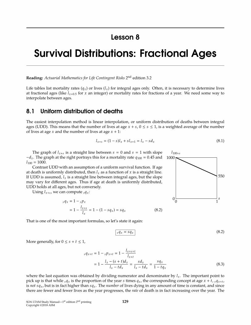
The easiest interpolation method is linear interpolation, or uniform distribution of deaths between integralages (UDD). This means that the number of lives at age x + s, 0 ≤ s ≤ 1, is a weighted average of the numberof lives at age x and the number of lives at age x + 1:
lx+s � (1 − s)lx + slx+1 � lx − sdx (8.1)
l100+s
1000
00 1s
550
The graph of lx+s is a straight line between s � 0 and s � 1 with slope−dx . The graph at the right portrays this for a mortality rate q100 � 0.45 andl100 � 1000.
Contrast UDDwith an assumption of a uniform survival function. If ageat death is uniformly distributed, then lx as a function of x is a straight line.If UDD is assumed, lx is a straight line between integral ages, but the slopemay vary for different ages. Thus if age at death is uniformly distributed,UDD holds at all ages, but not conversely.
Using lx+s , we can compute sqx :
s qx � 1 − s px
� 1 − lx+s
lx� 1 − (1 − sqx) � sqx (8.2)
That is one of the most important formulas, so let’s state it again:
s qx � sqx (8.2)
More generally, for 0 ≤ s + t ≤ 1,
s qx+t � 1 − s px+t � 1 − lx+s+t
lx+t
� 1 − lx − (s + t)dx
lx − tdx�
sdx
lx − tdx�
sqx
1 − tqx(8.3)
where the last equation was obtained by dividing numerator and denominator by lx . The important point topick up is that while s qx is the proportion of the year s times qx , the corresponding concept at age x + t, s qx+t ,is not sqx , but is in fact higher than sqx . The number of lives dying in any amount of time is constant, and sincethere are fewer and fewer lives as the year progresses, the rate of death is in fact increasing over the year. The
SOA LTAM Study Manual—1st edition 2nd printingCopyright ©2018 ASM
129
130 8. SURVIVAL DISTRIBUTIONS: FRACTIONAL AGES
numerator of s qx+t is the proportion of the year being measured s times the death rate, but then this must bedivided by 1 minus the proportion of the year that elapsed before the start of measurement.
For most problems involving death probabilities, it will suffice if you remember that lx+s is linearly interpo-lated. It often helps to create a life table with an arbitrary radix. Try working out the following example beforelooking at the answer.Example 8A You are given:
(i) qx � 0.1(ii) Uniform distribution of deaths between integral ages is assumed.
Calculate 1/2qx+1/4.
Answer: Let lx � 1. Then lx+1 � lx(1 − qx) � 0.9 and dx � 0.1. Linearly interpolating,
lx+1/4 � lx − 14 dx � 1 − 1
4 (0.1) � 0.975lx+3/4 � lx − 3
4 dx � 1 − 34 (0.1) � 0.925
1/2qx+1/4 �lx+1/4 − lx+3/4
lx+1/4�
0.975 − 0.9250.975 � 0.051282
You could also use equation (8.3) to work this example. �
Example 8B For two lives age (x)with independent future lifetimes, k |qx � 0.1(k + 1) for k � 0, 1, 2. Deaths areuniformly distributed between integral ages.
Calculate the probability that both lives will survive 2.25 years.
Answer: Since the two lives are independent, the probability of both surviving 2.25 years is the square of2.25px , the probability of one surviving 2.25 years. If we let lx � 1 and use dx+k � lx k |qx , we get
qx � 0.1(1) � 0.1 lx+1 � 1 − dx � 1 − 0.1 � 0.91|qx � 0.1(2) � 0.2 lx+2 � 0.9 − dx+1 � 0.9 − 0.2 � 0.72|qx � 0.1(3) � 0.3 lx+3 � 0.7 − dx+2 � 0.7 − 0.3 � 0.4
Then linearly interpolating between lx+2 and lx+3, we get
lx+2.25 � 0.7 − 0.25(0.3) � 0.625
2.25px �lx+2.25
lx� 0.625
Squaring, the answer is 0.6252 � 0.390625 . �
µ100+s
s
1
0
0.45
0.450.55
0 1
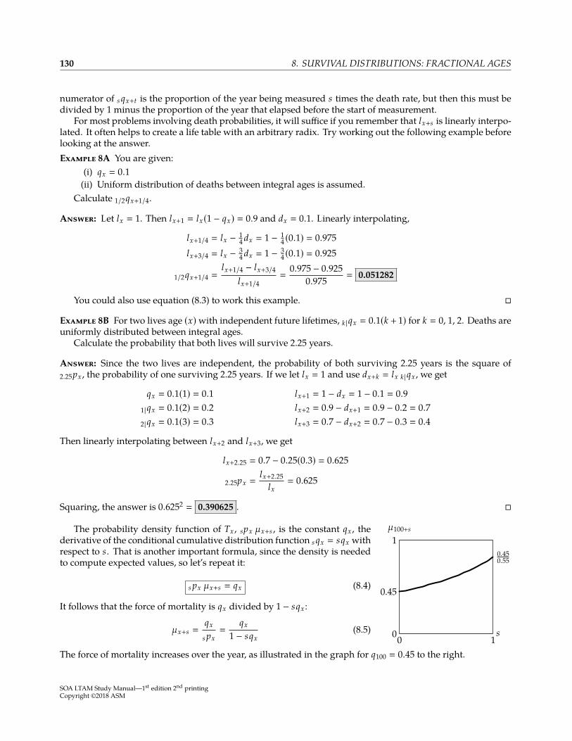
The probability density function of Tx , spx µx+s , is the constant qx , thederivative of the conditional cumulative distribution function s qx � sqx withrespect to s. That is another important formula, since the density is neededto compute expected values, so let’s repeat it:
s px µx+s � qx (8.4)
It follows that the force of mortality is qx divided by 1 − sqx :
µx+s �qx
s px�
qx
1 − sqx(8.5)
The force of mortality increases over the year, as illustrated in the graph for q100 � 0.45 to the right.
SOA LTAM Study Manual—1st edition 2nd printingCopyright ©2018 ASM

8.1. UNIFORM DISTRIBUTION OF DEATHS 131
?Quiz 8-1 You are given:(i) µ50.4 � 0.01(ii) Deaths are uniformly distributed between integral ages.
Calculate 0.6q50.4.
Complete Expectation of Life Under UDD
Under uniform distribution of deaths between integral ages, if the complete future lifetime random variable Txis written as Tx � Kx + Rx , where Kx is the curtate future lifetime and Rx is the fraction of the last year lived,then Kx and Rx are independent, and Rx is uniform on [0, 1). If uniform distribution of deaths is not assumed,Kx and Rx are usually not independent. Since Rx is uniform on [0, 1), E[Rx] � 1
2 and Var(Rx) � 112 . It follows
from E[Rx] � 12 that
ex � ex +12 (8.6)
Let’s discuss temporary complete life expectancy. You can always evaluate the temporary complete ex-pectancy, whether or not UDD is assumed, by integrating tpx , as indicated by formula (6.6) on page 84. ForUDD, t px is linear between integral ages. Therefore, a rule we learned in Lesson 6 applies for all integral x:
ex:1 � px + 0.5qx (6.13)
This equation will be useful. In addition, the method for generating this equation can be used to work outquestions involving temporary complete life expectancies for short periods. The following example illustratesthis. This example will be reminiscent of calculating temporary complete life expectancy for uniformmortality.
Example 8C You are given
(i) qx � 0.1.(ii) Deaths are uniformly distributed between integral ages.
Calculate ex:0.4 .
Answer: We will discuss two ways to solve this: an algebraic method and a geometric method.The algebraic method is based on the double expectation theorem, equation (1.14). It uses the fact that for
a uniform distribution, the mean is the midpoint. If deaths occur uniformly between integral ages, then those whodie within a period contained within a year survive half the period on the average.
In this example, those who die within 0.4 survive an average of 0.2. Those who survive 0.4 survive anaverage of 0.4 of course. The temporary life expectancy is the weighted average of these two groups, or0.4qx(0.2) + 0.4px(0.4). This is:
0.4qx � (0.4)(0.1) � 0.040.4px � 1 − 0.04 � 0.96
ex:0.4 � 0.04(0.2) + 0.96(0.4) � 0.392
An equivalent geometric method, the trapezoidal rule, is to draw the t px function from 0 to 0.4. The integralof t px is the area under the line, which is the area of a trapezoid: the average of the heights times the width.The following is the graph (not drawn to scale):
SOA LTAM Study Manual—1st edition 2nd printingCopyright ©2018 ASM

132 8. SURVIVAL DISTRIBUTIONS: FRACTIONAL AGES
A B
(0.4, 0.96)(1.0, 0.9)
0 0.4 1.0
1
t px
t
Trapezoid A is the area we are interested in. Its area is 12 (1 + 0.96)(0.4) � 0.392 . �
?Quiz 8-2 As in Example 8C, you are given(i) qx � 0.1.(ii) Deaths are uniformly distributed between integral ages.
Calculate ex+0.4:0.6 .
Let’s now work out an example in which the duration crosses an integral boundary.
Example 8D You are given:
(i) qx � 0.1(ii) qx+1 � 0.2(iii) Deaths are uniformly distributed between integral ages.
Calculate ex+0.5:1 .
Answer: Let’s start with the algebraic method. Since the mortality rate changes at x + 1, we must split thegroup into those who die before x + 1, those who die afterwards, and those who survive. Those who die beforex + 1 live 0.25 on the average since the period to x + 1 is length 0.5. Those who die after x + 1 live between 0.5and 1 years; the midpoint of 0.5 and 1 is 0.75, so they live 0.75 years on the average. Those who survive live 1year.
Now let’s calculate the probabilities.
0.5qx+0.5 �0.5(0.1)
1 − 0.5(0.1) �5
95
0.5px+0.5 � 1 − 595 �
9095
0.5|0.5qx+0.5 �
(9095
) (0.5(0.2)) � 9
95
1px+0.5 � 1 − 595 −
995 �
8195
These probabilities could also be calculated by setting up an lx table with radix 100 at age x and interpolating
SOA LTAM Study Manual—1st edition 2nd printingCopyright ©2018 ASM

8.1. UNIFORM DISTRIBUTION OF DEATHS 133
within it to get lx+0.5 and lx+1.5. Then
lx+1 � 0.9lx � 90lx+2 � 0.8lx+1 � 72
lx+0.5 � 0.5(90 + 100) � 95lx+1.5 � 0.5(72 + 90) � 81
0.5qx+0.5 � 1 − 9095 �
595
0.5|0.5qx+0.5 �90 − 81
95 �9
95
1px+0.5 �lx+1.5lx+0.5
�8195
Either way, we’re now ready to calculate ex+0.5:1 .
ex+0.5:1 �5(0.25) + 9(0.75) + 81(1)
95 �8995
For the geometric method we draw the following graph:
A B
(0.5, 9095
)(1.0, 8195
)
0x + 0.5
0.5x + 1
1.0x + 1.5
1
t px+0.5
t
The heights at x + 1 and x + 1.5 are as we computed above. Then we compute each area separately. The area ofA is 1
2(1 +
9095
) (0.5) � 18595(4) . The area of B is 1
2( 90
95 +8195
) (0.5) � 17195(4) . Adding them up, we get 185+171
95(4) �8995 . �
?Quiz 8-3 The probability that a battery fails by the end of the kth month is given in the following table:
kProbability of battery failure by
the end of month k1 0.052 0.203 0.60
Between integral months, time of failure for the battery is uniformly distributed.Calculate the expected amount of time the battery survives within 2.25 months.
To calculate ex:n in terms of ex:n when x and n are both integers, note that those who survive n yearscontribute the same to both. Those who die contribute an average of 1
2 more to ex:n since they die on theaverage in the middle of the year. Thus the difference is 1
2 n qx :
ex:n � ex:n + 0.5n qx (8.7)
SOA LTAM Study Manual—1st edition 2nd printingCopyright ©2018 ASM
134 8. SURVIVAL DISTRIBUTIONS: FRACTIONAL AGES
Example 8E You are given:(i) qx � 0.01 for x � 50, 51, . . . , 59.(ii) Deaths are uniformly distributed between integral ages.
Calculate e50:10 .
Answer: As we just said, e50:10 � e50:10 + 0.510q50. The first summand, e50:10 , is the sum of k p50 � 0.99k fork � 1, . . . , 10. This sum is a geometric series:
e50:10 �
10∑k�1
0.99k�
0.99 − 0.9911
1 − 0.99 � 9.46617
The second summand, the probability of dying within 10 years is 10q50 � 1 − 0.9910 � 0.095618. Therefore
e50:10 � 9.46617 + 0.5(0.095618) � 9.51398 �
8.2 Constant force of mortality
The constant force of mortality interpolation method sets µx+s equal to a constant for x an integral age and0 < s ≤ 1. Since px � exp
(−
∫ 10 µx+s ds
)and µx+s � µ is constant,
px � e−µ (8.8)µ � − ln px (8.9)
Thereforespx � e−µs
� (px)s (8.10)In fact, spx+t is independent of t for 0 ≤ t ≤ 1 − s.
spx+t � (px)s (8.11)
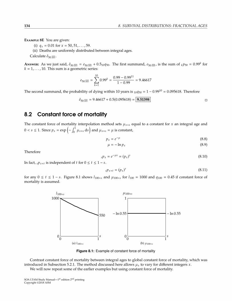
for any 0 ≤ t ≤ 1 − s. Figure 8.1 shows l100+s and µ100+s for l100 � 1000 and q100 � 0.45 if constant force ofmortality is assumed.
l100+s
1000
00 1s
550
(a) l100+s
µ100+s
s
1
00 1
− ln 0.55 − ln 0.55
(b) µ100+s
Figure 8.1: Example of constant force of mortality
Contrast constant force of mortality between integral ages to global constant force of mortality, which wasintroduced in Subsection 5.2.1. The method discussed here allows µx to vary for different integers x.
We will now repeat some of the earlier examples but using constant force of mortality.
SOA LTAM Study Manual—1st edition 2nd printingCopyright ©2018 ASM
EXERCISES FOR LESSON 8 135
Example 8F You are given:(i) qx � 0.1(ii) The force of mortality is constant between integral ages.
Calculate 1/2qx+1/4.
Answer:
1/2qx+1/4 � 1 − 1/2px+1/4 � 1 − p1/2x � 1 − 0.91/2
� 1 − 0.948683 � 0.051317 �
Example 8G You are given:(i) qx � 0.1(ii) qx+1 � 0.2(iii) The force of mortality is constant between integral ages.Calculate ex+0.5:1 .
Answer: We calculate∫ 1
0 t px+0.5 dt. We split this up into two integrals, one from 0 to 0.5 for age x and onefrom 0.5 to 1 for age x + 1. The first integral is∫ 0.5
0t px+0.5 dt �
∫ 0.5
0pt
x dt �∫ 0.5
00.9t dt � −1 − 0.90.5
ln 0.9 � 0.487058
For t > 0.5,t px+0.5 � 0.5px+0.5 t−0.5px+1 � 0.90.5
t−0.5px+1
so the second integral is
0.90.5∫ 1
0.5t−0.5px+1 dt � 0.90.5
∫ 0.5
00.8t dt � − (
0.90.5) (1 − 0.80.5
ln 0.8
)� (0.948683)(0.473116) � 0.448837
The answer is ex+0.5:1 � 0.487058 + 0.448837 � 0.935895 . �
Although constant force of mortality is not used as often as UDD, it can be useful for simplifying formulasunder certain circumstances. Calculating the expected present value of an insurance where the death benefitwithin a year follows an exponential pattern (this can happen when the death benefit is the discounted presentvalue of something) may be easier with constant force of mortality than with UDD. The formulas for this lessonare summarized in Table 8.1.
Exercises
Uniform distribution of death
8.1. [CAS4-S85:16] (1 point) Deaths are uniformly distributed between integral ages.Which of the following represents 3/4px +
12 1/2px µx+1/2?
(A) 3/4px (B) 3/4qx (C) 1/2px (D) 1/2qx (E) 1/4px
8.2. [Based on 150-S88:25] You are given:
(i) 0.25qx+0.75 � 3/31.(ii) Mortality is uniformly distributed within age x.
Calculate qx .
SOA LTAM Study Manual—1st edition 2nd printingCopyright ©2018 ASM
Exercises continue on the next page . . .
136 8. SURVIVAL DISTRIBUTIONS: FRACTIONAL AGES
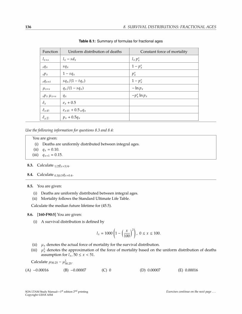
Table 8.1: Summary of formulas for fractional ages
Function Uniform distribution of deaths Constant force of mortality
lx+s lx − sdx lx psx
sqx sqx 1 − psx
spx 1 − sqx psx
sqx+t sqx/(1 − tqx) 1 − psx
µx+s qx/(1 − sqx) − ln px
spx µx+s qx −psx ln px
ex ex + 0.5
ex:n ex:n + 0.5 n qx
ex:1 px + 0.5qx
Use the following information for questions 8.3 and 8.4:
You are given:(i) Deaths are uniformly distributed between integral ages.(ii) qx � 0.10.(iii) qx+1 � 0.15.
8.3. Calculate 1/2qx+3/4.
8.4. Calculate 0.3|0.5qx+0.4.
8.5. You are given:
(i) Deaths are uniformly distributed between integral ages.(ii) Mortality follows the Standard Ultimate Life Table.
Calculate the median future lifetime for (45.5).
8.6. [160-F90:5] You are given:
(i) A survival distribution is defined by
lx � 1000(1 −
( x100
)2), 0 ≤ x ≤ 100.
(ii) µx denotes the actual force of mortality for the survival distribution.(iii) µL
x denotes the approximation of the force of mortality based on the uniform distribution of deathsassumption for lx , 50 ≤ x < 51.
Calculate µ50.25 − µL50.25.
(A) −0.00016 (B) −0.00007 (C) 0 (D) 0.00007 (E) 0.00016
SOA LTAM Study Manual—1st edition 2nd printingCopyright ©2018 ASM
Exercises continue on the next page . . .
EXERCISES FOR LESSON 8 137
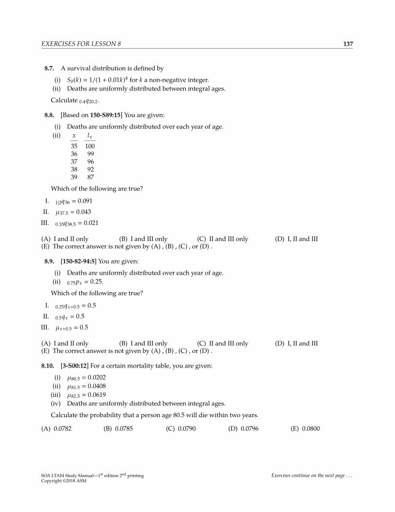
8.7. A survival distribution is defined by
(i) S0(k) � 1/(1 + 0.01k)4 for k a non-negative integer.(ii) Deaths are uniformly distributed between integral ages.
Calculate 0.4q20.2.
8.8. [Based on 150-S89:15] You are given:
(i) Deaths are uniformly distributed over each year of age.(ii) x lx
35 10036 9937 9638 9239 87
Which of the following are true?
I. 1|2q36 � 0.091II. µ37.5 � 0.043III. 0.33q38.5 � 0.021
(A) I and II only (B) I and III only (C) II and III only (D) I, II and III(E) The correct answer is not given by (A) , (B) , (C) , or (D) .
8.9. [150-82-94:5] You are given:
(i) Deaths are uniformly distributed over each year of age.(ii) 0.75px � 0.25.
Which of the following are true?
I. 0.25qx+0.5 � 0.5II. 0.5qx � 0.5III. µx+0.5 � 0.5
(A) I and II only (B) I and III only (C) II and III only (D) I, II and III(E) The correct answer is not given by (A) , (B) , (C) , or (D) .
8.10. [3-S00:12] For a certain mortality table, you are given:
(i) µ80.5 � 0.0202(ii) µ81.5 � 0.0408(iii) µ82.5 � 0.0619(iv) Deaths are uniformly distributed between integral ages.
Calculate the probability that a person age 80.5 will die within two years.
(A) 0.0782 (B) 0.0785 (C) 0.0790 (D) 0.0796 (E) 0.0800
SOA LTAM Study Manual—1st edition 2nd printingCopyright ©2018 ASM
Exercises continue on the next page . . .
138 8. SURVIVAL DISTRIBUTIONS: FRACTIONAL AGES
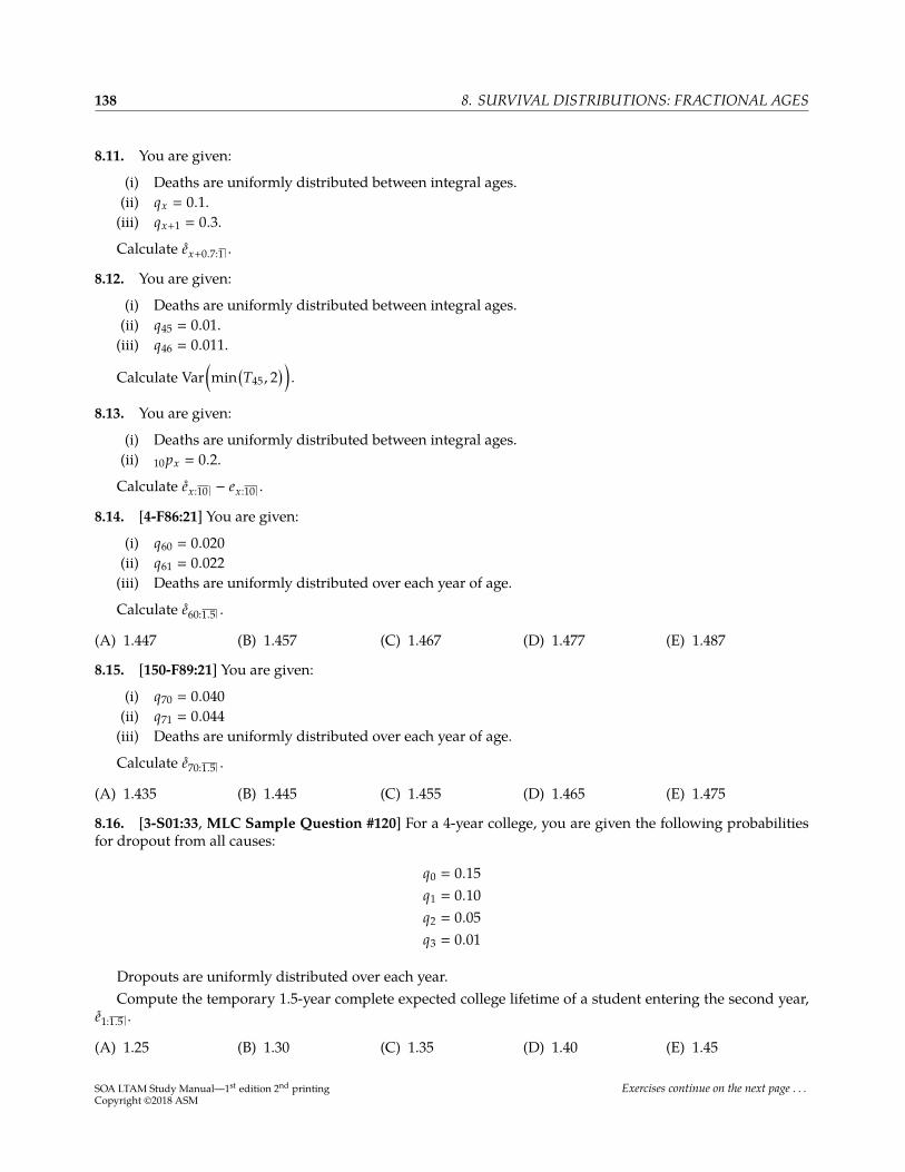
8.11. You are given:
(i) Deaths are uniformly distributed between integral ages.(ii) qx � 0.1.(iii) qx+1 � 0.3.
Calculate ex+0.7:1 .
8.12. You are given:
(i) Deaths are uniformly distributed between integral ages.(ii) q45 � 0.01.(iii) q46 � 0.011.
Calculate Var(min
(T45 , 2
) ).
8.13. You are given:
(i) Deaths are uniformly distributed between integral ages.(ii) 10px � 0.2.
Calculate ex:10 − ex:10 .
8.14. [4-F86:21] You are given:
(i) q60 � 0.020(ii) q61 � 0.022(iii) Deaths are uniformly distributed over each year of age.
Calculate e60:1.5 .
(A) 1.447 (B) 1.457 (C) 1.467 (D) 1.477 (E) 1.487
8.15. [150-F89:21] You are given:
(i) q70 � 0.040(ii) q71 � 0.044(iii) Deaths are uniformly distributed over each year of age.
Calculate e70:1.5 .
(A) 1.435 (B) 1.445 (C) 1.455 (D) 1.465 (E) 1.475
8.16. [3-S01:33, MLC Sample Question #120] For a 4-year college, you are given the following probabilitiesfor dropout from all causes:
q0 � 0.15q1 � 0.10q2 � 0.05q3 � 0.01
Dropouts are uniformly distributed over each year.Compute the temporary 1.5-year complete expected college lifetime of a student entering the second year,
e1:1.5 .
(A) 1.25 (B) 1.30 (C) 1.35 (D) 1.40 (E) 1.45
SOA LTAM Study Manual—1st edition 2nd printingCopyright ©2018 ASM
Exercises continue on the next page . . .
EXERCISES FOR LESSON 8 139
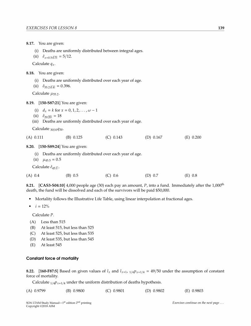
8.17. You are given:
(i) Deaths are uniformly distributed between integral ages.(ii) ex+0.5:0.5 � 5/12.
Calculate qx .
8.18. You are given:
(i) Deaths are uniformly distributed over each year of age.(ii) e55.2:0.4 � 0.396.
Calculate µ55.2.
8.19. [150-S87:21] You are given:
(i) dx � k for x � 0, 1, 2, . . . , ω − 1(ii) e20:20 � 18(iii) Deaths are uniformly distributed over each year of age.
Calculate 30|10q30.
(A) 0.111 (B) 0.125 (C) 0.143 (D) 0.167 (E) 0.200
8.20. [150-S89:24] You are given:
(i) Deaths are uniformly distributed over each year of age.(ii) µ45.5 � 0.5
Calculate e45:1 .
(A) 0.4 (B) 0.5 (C) 0.6 (D) 0.7 (E) 0.8
8.21. [CAS3-S04:10] 4,000 people age (30) each pay an amount, P, into a fund. Immediately after the 1,000thdeath, the fund will be dissolved and each of the survivors will be paid $50,000.
• Mortality follows the Illustrative Life Table, using linear interpolation at fractional ages.
• i � 12%
Calculate P.(A) Less than 515(B) At least 515, but less than 525(C) At least 525, but less than 535(D) At least 535, but less than 545(E) At least 545
Constant force of mortality
8.22. [160-F87:5] Based on given values of lx and lx+1, 1/4px+1/4 � 49/50 under the assumption of constantforce of mortality.
Calculate 1/4px+1/4 under the uniform distribution of deaths hypothesis.
(A) 0.9799 (B) 0.9800 (C) 0.9801 (D) 0.9802 (E) 0.9803
SOA LTAM Study Manual—1st edition 2nd printingCopyright ©2018 ASM
Exercises continue on the next page . . .
140 8. SURVIVAL DISTRIBUTIONS: FRACTIONAL AGES
8.23. [160-S89:5] A mortality study is conducted for the age interval (x , x + 1].If a constant force of mortality applies over the interval, 0.25qx+0.1 � 0.05.Calculate 0.25qx+0.1 assuming a uniform distribution of deaths applies over the interval.
(A) 0.044 (B) 0.047 (C) 0.050 (D) 0.053 (E) 0.056
8.24. [150-F89:29] You are given that qx � 0.25.Based on the constant force of mortality assumption, the force of mortality is µA
x+s , 0 < s < 1.Based on the uniform distribution of deaths assumption, the force of mortality is µB
x+s , 0 < s < 1.Calculate the smallest s such that µB
x+s ≥ µAx+s .
(A) 0.4523 (B) 0.4758 (C) 0.5001 (D) 0.5239 (E) 0.5477
8.25. [160-S91:4] From a population mortality study, you are given:
(i) Within each age interval, [x + k , x + k + 1), the force of mortality, µx+k , is constant.
(ii) k e−µx+k1 − e−µx+k
µx+k
0 0.98 0.991 0.96 0.98
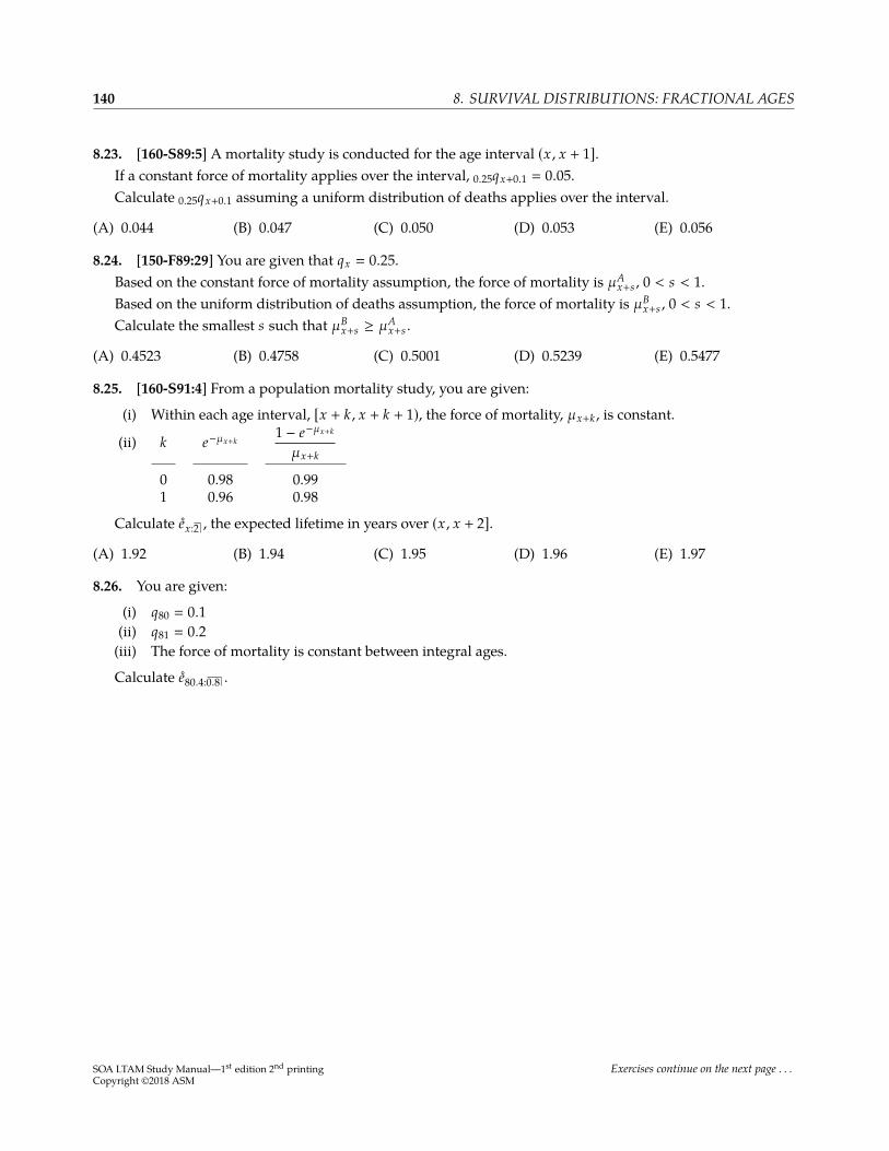
Calculate ex:2 , the expected lifetime in years over (x , x + 2].(A) 1.92 (B) 1.94 (C) 1.95 (D) 1.96 (E) 1.97
8.26. You are given:
(i) q80 � 0.1(ii) q81 � 0.2(iii) The force of mortality is constant between integral ages.
Calculate e80.4:0.8 .
SOA LTAM Study Manual—1st edition 2nd printingCopyright ©2018 ASM
Exercises continue on the next page . . .
EXERCISES FOR LESSON 8 141
8.27. [3-S01:27] An actuary is modeling the mortality of a group of 1000 people, each age 95, for the next threeyears.
The actuary starts by calculating the expected number of survivors at each integral age by
l95+k � 1000 k p95 , k � 1, 2, 3
The actuary subsequently calculates the expected number of survivors at the middle of each year using theassumption that deaths are uniformly distributed over each year of age.
This is the result of the actuary’s model:
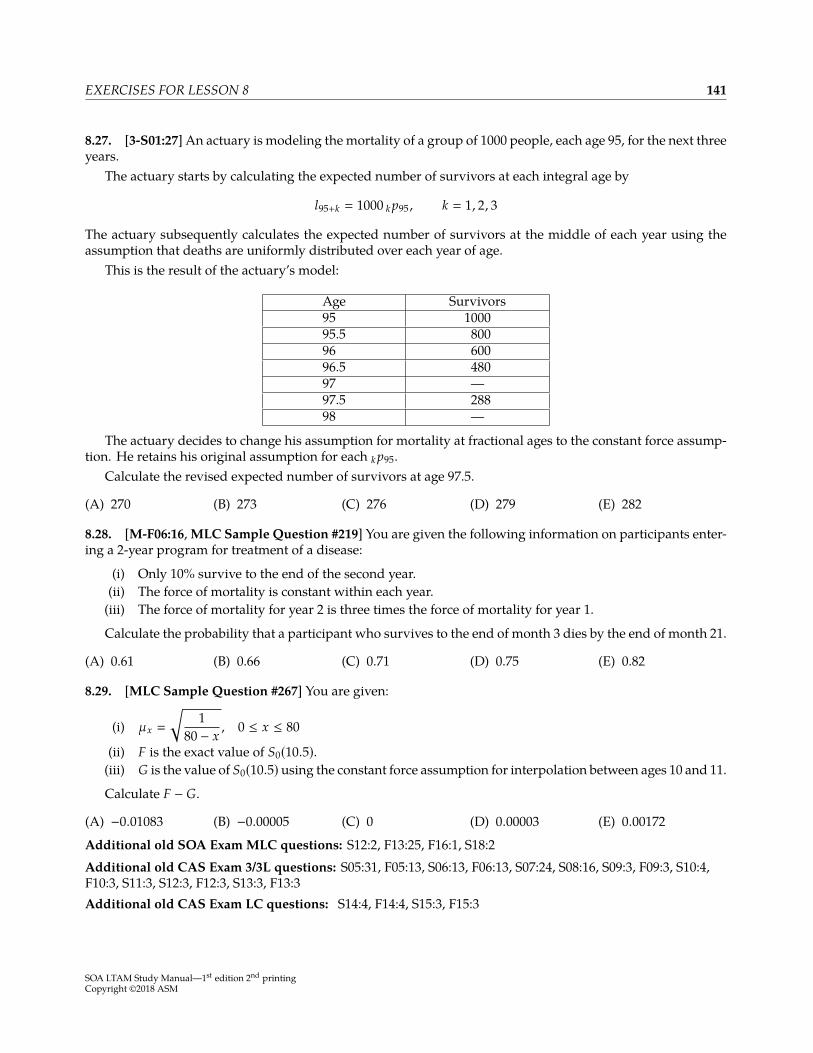
Age Survivors95 100095.5 80096 60096.5 48097 —97.5 28898 —
The actuary decides to change his assumption for mortality at fractional ages to the constant force assump-tion. He retains his original assumption for each k p95.
Calculate the revised expected number of survivors at age 97.5.
(A) 270 (B) 273 (C) 276 (D) 279 (E) 282
8.28. [M-F06:16,MLC Sample Question #219] You are given the following information on participants enter-ing a 2-year program for treatment of a disease:
(i) Only 10% survive to the end of the second year.(ii) The force of mortality is constant within each year.(iii) The force of mortality for year 2 is three times the force of mortality for year 1.
Calculate the probability that a participant who survives to the end of month 3 dies by the end of month 21.
(A) 0.61 (B) 0.66 (C) 0.71 (D) 0.75 (E) 0.82
8.29. [MLC Sample Question #267] You are given:
(i) µx �
√1
80 − x, 0 ≤ x ≤ 80
(ii) F is the exact value of S0(10.5).(iii) G is the value of S0(10.5) using the constant force assumption for interpolation between ages 10 and 11.
Calculate F − G.
(A) −0.01083 (B) −0.00005 (C) 0 (D) 0.00003 (E) 0.00172
Additional old SOA ExamMLC questions: S12:2, F13:25, F16:1, S18:2Additional old CAS Exam 3/3L questions: S05:31, F05:13, S06:13, F06:13, S07:24, S08:16, S09:3, F09:3, S10:4,F10:3, S11:3, S12:3, F12:3, S13:3, F13:3Additional old CAS Exam LC questions: S14:4, F14:4, S15:3, F15:3
SOA LTAM Study Manual—1st edition 2nd printingCopyright ©2018 ASM
142 8. SURVIVAL DISTRIBUTIONS: FRACTIONAL AGES
Solutions
8.1. In the second summand, 1/2px µx+1/2 is the density function, which is the constant qx under UDD. Thefirst summand 3/4px � 1 − 3
4 qx . So the sum is 1 − 14 qx , or 1/4px . (E)
8.2. Using equation (8.3),
331 � 0.25qx+0.75 �
0.25qx
1 − 0.75qx
331 −
2.2531 qx � 0.25qx
331 �
1031 qx
qx � 0.3
8.3. We calculate the probability that (x +34 ) survives for half a year. Since the duration crosses an integer
boundary, we break the period up into two quarters of a year. The probability of (x + 3/4) surviving for 0.25years is, by equation (8.3),
1/4px+3/4 �1 − 0.10
1 − 0.75(0.10) �0.9
0.925The probability of (x + 1) surviving to x + 1.25 is
1/4px+1 � 1 − 0.25(0.15) � 0.9625
The answer to the question is then the complement of the product of these two numbers:
1/2qx+3/4 � 1 − 1/2px+3/4 � 1 − 1/4px+3/4 1/4px+1 � 1 −(
0.90.925
)(0.9625) � 0.06351
Alternatively, you could build a life table starting at age x, with lx � 1. Then lx+1 � (1 − 0.1) � 0.9 andlx+2 � 0.9(1 − 0.15) � 0.765. Under UDD, lx at fractional ages is obtained by linear interpolation, so
lx+0.75 � 0.75(0.9) + 0.25(1) � 0.925lx+1.25 � 0.25(0.765) + 0.75(0.9) � 0.86625
1/2p3/4 �lx+1.25lx+0.75
�0.866250.925 � 0.93649
1/2q3/4 � 1 − 1/2p3/4 � 1 − 0.93649 � 0.06351
8.4. 0.3|0.5qx+0.4 is 0.3px+0.4 − 0.8px+0.4. The first summand is
0.3px+0.4 �1 − 0.7qx
1 − 0.4qx�
1 − 0.071 − 0.04 �
9396
The probability that (x + 0.4) survives to x + 1 is, by equation (8.3),
0.6px+0.4 �1 − 0.101 − 0.04 �
9096
and the probability (x + 1) survives to x + 1.2 is
0.2px+1 � 1 − 0.2qx+1 � 1 − 0.2(0.15) � 0.97
SOA LTAM Study Manual—1st edition 2nd printingCopyright ©2018 ASM
EXERCISE SOLUTIONS FOR LESSON 8 143
So
0.3|0.5qx+0.4 �9396 −
(9096
)(0.97) � 0.059375
Alternatively, you could use the life table from the solution to the last question, and linearly interpolate:
lx+0.4 � 0.4(0.9) + 0.6(1) � 0.96lx+0.7 � 0.7(0.9) + 0.3(1) � 0.93lx+1.2 � 0.2(0.765) + 0.8(0.9) � 0.873
0.3|0.5qx+0.4 �0.93 − 0.873
0.96 � 0.059375
8.5. Under uniform distribution of deaths between integral ages, lx+0.5 �12 (lx + lx+1), since the survival
function is a straight line between two integral ages. Therefore, l45.5 �12 (99,033.9 + 98,957.6) � 98,995.75.
Median future lifetime occurs when lx �12 (98,995.75) � 49,497.9. This happens between ages 88 and 89. We
interpolate between the ages to get the exact median:
l88 − s(l88 − l89) � 49,497.950,038.6 − s(50,038.6 − 45,995.6) � 49,497.9
50,038.6 − 4,043.0s � 49,497.9
s �50,038.6 − 49,497.9
4,043.0 � 0.08080
So the median age at death is 88.08080, and median future lifetime is 88.08080 − 45.5 � 43.08080 .
8.6. x p0 �lxl0� 1 − ( x
100)2. The force of mortality is calculated as the negative derivative of ln x p0:
µx � −d ln x p0
dx�
2( x100
) ( 1100
)1 − ( x
100)2 �
2x1002 − x2
µ50.25 �100.5
1002 − 50.252 � 0.0134449
For UDD, we need to calculate q50.
p50 �l51l50
�1 − 0.512
1 − 0.502 � 0.986533
q50 � 1 − 0.986533 � 0.013467
so under UDD,µL
50.25 �q50
1 − 0.25q50�
0.0134671 − 0.25(0.013467) � 0.013512.
The difference between µ50.25 and µL50.25 is 0.013445 − 0.013512 � −0.000067 . (B)
8.7. S0(20) � 1/1.24 and S0(21) � 1/1.214, so q20 � 1 − (1.2/1.21)4 � 0.03265. Then
0.4q20.2 �0.4q20
1 − 0.2q20�
0.4(0.03265)1 − 0.2(0.03265) � 0.01315
SOA LTAM Study Manual—1st edition 2nd printingCopyright ©2018 ASM
144 8. SURVIVAL DISTRIBUTIONS: FRACTIONAL AGES
8.8.I. Calculate 1|2q36.
1|2q36 �2d37l36
�96 − 87
99 � 0.09091 !
This statement does not require uniform distribution of deaths.II. By equation (8.5),
µ37.5 �q37
1 − 0.5q37�
4/961 − 2/96
�4
94 � 0.042553 !
III. Calculate 0.33q38.5.
0.33q38.5 �0.33d38.5
l38.5�(0.33)(5)
89.5 � 0.018436 #
I can’t figure out what mistake you’d have to make to get 0.021. (A)
8.9. First calculate qx .
1 − 0.75qx � 0.25qx � 1
Then by equation (8.3), 0.25qx+0.5 � 0.25/(1 − 0.5) � 0.5, making I true.By equation (8.2), 0.5qx � 0.5qx � 0.5, making II true.By equation (8.5), µx+0.5 � 1/(1 − 0.5) � 2, making III false. (A)
8.10. We use equation (8.5) to back out qx for each age.
µx+0.5 �qx
1 − 0.5qx⇒ qx �
µx+0.5
1 + 0.5µx+0.5
q80 �0.02021.0101 � 0.02
q81 �0.04081.0204 � 0.04
q82 �0.0619
1.03095 � 0.06
Then by equation (8.3), 0.5p80.5 � 0.98/0.99. p81 � 0.96, and 0.5p82 � 1 − 0.5(0.06) � 0.97. Therefore
2q80.5 � 1 −(0.980.99
)(0.96)(0.97) � 0.0782 (A)
8.11. To do this algebraically, we split the group into those who die within 0.3 years, those who die between0.3 and 1 years, and those who survive one year. Under UDD, those who die will die at the midpoint of theinterval (assuming the interval doesn’t cross an integral age), so we have
Survival Probability AverageGroup time of group survival time
I (0, 0.3] 1 − 0.3px+0.7 0.15II (0.3, 1] 0.3px+0.7 − 1px+0.7 0.65III (1,∞) 1px+0.7 1
We calculate the required probabilities.
0.3px+0.7 �0.90.93 � 0.967742
SOA LTAM Study Manual—1st edition 2nd printingCopyright ©2018 ASM
EXERCISE SOLUTIONS FOR LESSON 8 145
1px+0.7 �0.90.93
(1 − 0.7(0.3)) � 0.764516
1 − 0.3px+0.7 � 1 − 0.967742 � 0.0322580.3px+0.7 − 1px+0.7 � 0.967742 − 0.764516 � 0.203226
ex+0.7:1 � 0.032258(0.15) + 0.203226(0.65) + 0.764516(1) � 0.901452
Alternatively, we can use trapezoids. We already know from the above solution that the heights of the firsttrapezoid are 1 and 0.967742, and the heights of the second trapezoid are 0.967742 and 0.764516. So the sum ofthe area of the two trapezoids is
ex+0.7:1 � (0.3)(0.5)(1 + 0.967742) + (0.7)(0.5)(0.967742 + 0.764516)� 0.295161 + 0.606290 � 0.901451
8.12. For the expected value, we’ll use the recursive formula. (The trapezoidal rule could also be used.)
e45:2 � e45:1 + p45 e46:1� (1 − 0.005) + 0.99(1 − 0.0055)� 1.979555
We’ll use equation (6.7)to calculate the second moment.
E[min(T45 , 2)2] � 2∫ 2
0t t px dt
� 2(∫ 1
0t(1 − 0.01t)dt +
∫ 2
1t(0.99)(1 − 0.011(t − 1)) dt
)
� 2 ©«12 − 0.01
(13
)+ 0.99
((1.011)(22 − 12)
2 − 0.011(23 − 13
3
))ª®¬� 2(0.496667 + 1.475925) � 3.94518
So the variance is 3.94518 − 1.9795552 � 0.02654 .8.13. As discussed on page 133, by equation (8.7), the difference is
12 10qx �
12 (1 − 0.2) � 0.4
8.14. Those who die in the first year survive 12 year on the average and those who die in the first half of the
second year survive 1.25 years on the average, so we have
p60 � 0.98
1.5p60 � 0.98(1 − 0.5(0.022)) � 0.96922
e60:1.5 � 0.5(0.02) + 1.25(0.98 − 0.96922) + 1.5(0.96922) � 1.477305 (D)
Alternatively, we use the trapezoidal method. The first trapezoid has heights 1 and p60 � 0.98 andwidth 1.The second trapezoid has heights p60 � 0.98 and 1.5p60 � 0.96922 and width 1/2.
e60:1.5 �12 (1 + 0.98) +
(12
) (12
)(0.98 + 0.96922)
� 1.477305 (D)
SOA LTAM Study Manual—1st edition 2nd printingCopyright ©2018 ASM
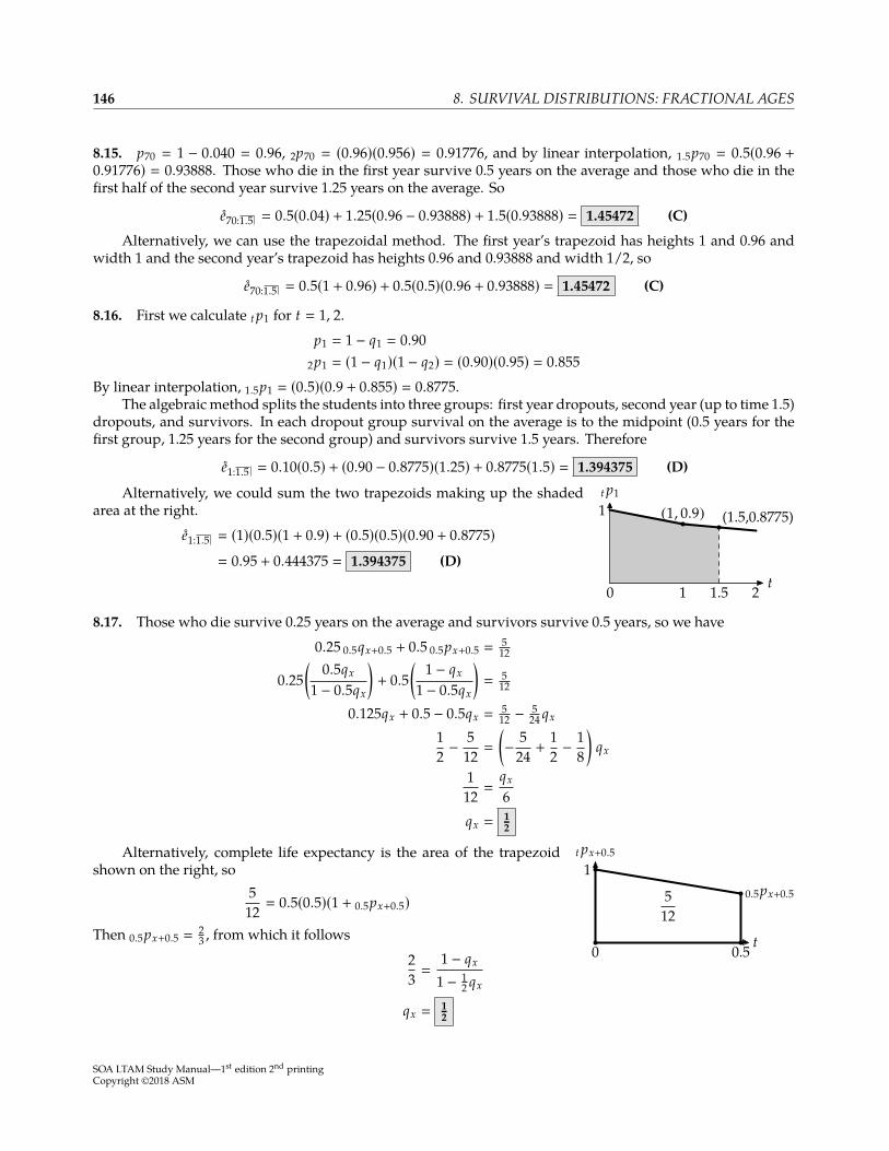
146 8. SURVIVAL DISTRIBUTIONS: FRACTIONAL AGES
8.15. p70 � 1 − 0.040 � 0.96, 2p70 � (0.96)(0.956) � 0.91776, and by linear interpolation, 1.5p70 � 0.5(0.96 +
0.91776) � 0.93888. Those who die in the first year survive 0.5 years on the average and those who die in thefirst half of the second year survive 1.25 years on the average. So
e70:1.5 � 0.5(0.04) + 1.25(0.96 − 0.93888) + 1.5(0.93888) � 1.45472 (C)
Alternatively, we can use the trapezoidal method. The first year’s trapezoid has heights 1 and 0.96 andwidth 1 and the second year’s trapezoid has heights 0.96 and 0.93888 and width 1/2, so
e70:1.5 � 0.5(1 + 0.96) + 0.5(0.5)(0.96 + 0.93888) � 1.45472 (C)
8.16. First we calculate t p1 for t � 1, 2.p1 � 1 − q1 � 0.90
2p1 � (1 − q1)(1 − q2) � (0.90)(0.95) � 0.855By linear interpolation, 1.5p1 � (0.5)(0.9 + 0.855) � 0.8775.
The algebraic method splits the students into three groups: first year dropouts, second year (up to time 1.5)dropouts, and survivors. In each dropout group survival on the average is to the midpoint (0.5 years for thefirst group, 1.25 years for the second group) and survivors survive 1.5 years. Therefore
e1:1.5 � 0.10(0.5) + (0.90 − 0.8775)(1.25) + 0.8775(1.5) � 1.394375 (D)
0 1 1.5 2
1
t
t p1
(1, 0.9) (1.5,0.8775)Alternatively, we could sum the two trapezoids making up the shaded
area at the right.e1:1.5 � (1)(0.5)(1 + 0.9) + (0.5)(0.5)(0.90 + 0.8775)
� 0.95 + 0.444375 � 1.394375 (D)
8.17. Those who die survive 0.25 years on the average and survivors survive 0.5 years, so we have0.25 0.5qx+0.5 + 0.5 0.5px+0.5 �
512
0.25(
0.5qx
1 − 0.5qx
)+ 0.5
(1 − qx
1 − 0.5qx
)�
512
0.125qx + 0.5 − 0.5qx �512 − 5
24 qx
12 −
512 �
(− 5
24 +12 −
18
)qx
112 �
qx
6qx �
12
512
0 0.5 t
t px+0.5
10.5px+0.5
Alternatively, complete life expectancy is the area of the trapezoidshown on the right, so
512 � 0.5(0.5)(1 + 0.5px+0.5)
Then 0.5px+0.5 �23 , from which it follows
23 �
1 − qx
1 − 12 qx
qx �12
SOA LTAM Study Manual—1st edition 2nd printingCopyright ©2018 ASM
EXERCISE SOLUTIONS FOR LESSON 8 147
8.18. Survivors live 0.4 years and those who die live 0.2 years on the average, so
0.396 � 0.40.4p55.2 + 0.20.4q55.2
Using the formula 0.4q55.2 � 0.4q55/(1 − 0.2q55) (equation (8.3)), we have
0.4(1 − 0.6q55
1 − 0.2q55
)+ 0.2
(0.4q55
1 − 0.2q55
)� 0.396
0.4 − 0.24q55 + 0.08q55 � 0.396 − 0.0792q55
0.0808q55 � 0.004
q55 �0.004
0.0808 � 0.0495
µ55.2 �q55
1 − 0.2q55�
0.04951 − 0.2(0.0495) � 0.05
8.19. Since dx is constant for all x and deaths are uniformly distributed within each year of age, mortality isuniform globally. We back out ω using equation (6.12), ex:n � n px(n) + n qx(n/2):
10 20q20 + 20 20p20 � 18
10(
20ω − 20
)+ 20
(ω − 40ω − 20
)� 18
200 + 20ω − 800 � 18ω − 3602ω � 240ω � 120
18
20 40x
x−20p20
1ω − 40ω − 20
Alternatively, we can back out ω using the trapezoidal rule. Completelife expectancy is the area of the trapezoid shown to the right.
e20:20 � 18 � (20)(0.5)(1 +
ω − 40ω − 20
)
0.8 �ω − 40ω − 20
0.8ω − 16 � ω − 400.2ω � 24ω � 120
Once we have ω, we compute
30|10q30 �10
ω − 30 �1090 � 0.1111 (A)
8.20. We use equation (8.5) to obtain
0.5 �qx
1 − 0.5qx
qx � 0.4
Then e45:1 � 0.5(1 + (1 − 0.4)) � 0.8 . (E)
SOA LTAM Study Manual—1st edition 2nd printingCopyright ©2018 ASM
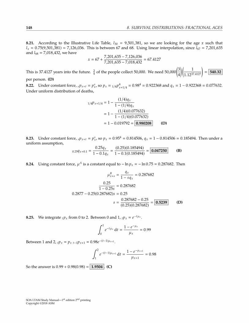
148 8. SURVIVAL DISTRIBUTIONS: FRACTIONAL AGES
8.21. According to the Illustrative Life Table, l30 � 9,501,381, so we are looking for the age x such thatlx � 0.75(9,501,381) � 7,126,036. This is between 67 and 68. Using linear interpolation, since l67 � 7,201,635and l68 � 7,018,432, we have
x � 67 +7,201,635 − 7,126,0367,201,635 − 7,018,432 � 67.4127
This is 37.4127 years into the future. 34 of the people collect 50,000. We need 50,000
(34
) (1
1.1237.4127
)� 540.32
per person. (D)8.22. Under constant force, s px+t � ps
x , so px � 1/4p4x+1/4 � 0.984 � 0.922368 and qx � 1 − 0.922368 � 0.077632.
Under uniform distribution of deaths,
1/4px+1/4 � 1 − (1/4)qx
1 − (1/4)qx
� 1 − (1/4)(0.077632)1 − (1/4)(0.077632)
� 1 − 0.019792 � 0.980208 (D)
8.23. Under constant force, spx+t � psx , so px � 0.954 � 0.814506, qx � 1 − 0.814506 � 0.185494. Then under a
uniform assumption,
0.25qx+0.1 �0.25qx
1 − 0.1qx�(0.25)(0.185494)1 − 0.1(0.185494) � 0.047250 (B)
8.24. Using constant force, µA is a constant equal to − ln px � − ln 0.75 � 0.287682. Then
µBx+s �
qx
1 − sqx� 0.287682
0.251 − 0.25s
� 0.287682
0.2877 − 0.25(0.287682)s � 0.25
s �0.287682 − 0.25(0.25)(0.287682) � 0.5239 (D)
8.25. We integrate t px from 0 to 2. Between 0 and 1, tpx � e−tµx .∫ 1
0e−tµx dt �
1 − e−µx
µx� 0.99
Between 1 and 2, tpx � px t−1px+1 � 0.98e−(t−1)µx+1 .∫ 2
1e−(t−1)µx+1 dt �
1 − e−µx+1
µx+1� 0.98
So the answer is 0.99 + 0.98(0.98) � 1.9504 . (C)
SOA LTAM Study Manual—1st edition 2nd printingCopyright ©2018 ASM

QUIZ SOLUTIONS FOR LESSON 8 149
8.26.
e80.4:0.8 � e80.4:0.6 + 0.6p80.4 e81:0.2
�
∫ 10.4 0.9tdt
0.90.4 + 0.90.6∫ 0.2
00.8tdt
�0.90.6 − 1
ln 0.9 +(0.90.6) 0.80.2 − 1
ln 0.8� 0.581429 + (0.938740)(0.195603) � 0.765049
8.27. Under uniform distribution, the numbers of deaths in each half of the year are equal, so if 120 deathsoccurred in the first half of x � 96, then 120 occurred in the second half, and l97 � 480 − 120 � 360. Then if0.5q97 � (360 − 288)/360 � 0.2, then q97 � 2 0.5q97 � 0.4, so p97 � 0.6. Under constant force, 1/2p97 � p0.5
97 �√
0.6.The answer is 360
√0.6 � 278.8548 . (D)
8.28. Let µ be the force of mortality in year 1. Then 10% survivorship means
e−µ−3µ� 0.1
e−4µ� 0.1
The probability of survival 21 months given survival 3 months is the probability of survival 9 months aftermonth 3, or e−(3/4)µ, times the probability of survival another 9 months given survival 1 year, or e−(3/4)3µ, whichmultiplies to e−3µ � (e−4µ)3/4 � 0.13/4 � 0.177828, so the death probability is 1 − 0.177828 � 0.822172 . (E)8.29. The exact value is:
F � 10.5p0 � exp(−
∫ 10.5
0µx dx
)∫ 10.5
0(80 − x)−0.5dx � −2(80 − x)0.5��10.5
0
� −2(69.50.5 − 800.5)
� 1.215212
10.5p0 � e−1.215212� 0.296647
To calculate S0(10.5) with constant force interpolation between 10 and 11, we have 0.5p10 � p0.510 , and 10.5p0 �
10p0 0.5p10, so ∫ 10
0(80 − x)−0.5dx � −2
(700.5 − 800.5)
� 1.155343∫ 11
10(80 − x)−0.5dx � −2
(690.5 − 700.5)
� 0.119953
G � 10.5p0 � e−1.155343−0.5(0.119953)� 0.296615
Then F − G � 0.296647 − 0.296615 � 0.000032 . (D)
Quiz Solutions
8-1. Notice that µ50.4 �q50
1−0.4q50while 0.6q50.4 �
0.6q501−0.4q50
, so 0.6q50.4 � 0.6(0.01) � 0.006
SOA LTAM Study Manual—1st edition 2nd printingCopyright ©2018 ASM
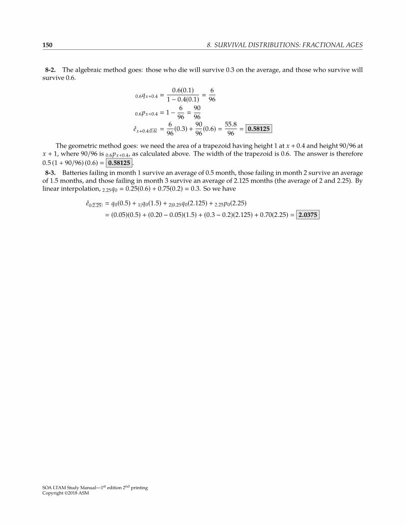
150 8. SURVIVAL DISTRIBUTIONS: FRACTIONAL AGES
8-2. The algebraic method goes: those who die will survive 0.3 on the average, and those who survive willsurvive 0.6.
0.6qx+0.4 �0.6(0.1)
1 − 0.4(0.1) �6
96
0.6px+0.4 � 1 − 696 �
9096
ex+0.4:0.6 �6
96 (0.3) +9096 (0.6) �
55.896 � 0.58125
The geometric method goes: we need the area of a trapezoid having height 1 at x + 0.4 and height 90/96 atx + 1, where 90/96 is 0.6px+0.4, as calculated above. The width of the trapezoid is 0.6. The answer is therefore0.5 (1 + 90/96) (0.6) � 0.58125 .8-3. Batteries failing in month 1 survive an average of 0.5 month, those failing in month 2 survive an averageof 1.5 months, and those failing in month 3 survive an average of 2.125 months (the average of 2 and 2.25). Bylinear interpolation, 2.25q0 � 0.25(0.6) + 0.75(0.2) � 0.3. So we have
e0:2.25 � q0(0.5) + 1|q0(1.5) + 2|0.25q0(2.125) + 2.25p0(2.25)� (0.05)(0.5) + (0.20 − 0.05)(1.5) + (0.3 − 0.2)(2.125) + 0.70(2.25) � 2.0375
SOA LTAM Study Manual—1st edition 2nd printingCopyright ©2018 ASM

Practice Exam 1
SECTION A—Multiple-Choice
1. A life age 60 is subject to Gompertz’s law with B � 0.001 and c � 1.05.Calculate e60:2 for this life.
(A) 1.923 (B) 1.928 (C) 1.933 (D) 1.938 (E) 1.943
2. Your company sells whole life insurance policies. At a meeting with the Enterprise Risk ManagementCommittee, it was agreed that you would limit the face amount of the policies sold so that the probability thatthe present value of the benefit at issue is greater than 1,000,000 is never more than 0.05.
You are given:
(i) The insurance policies pay a benefit equal to the face amount b at the moment of death.(ii) The force of mortality is µx � 0.001(1.05x), x > 0(iii) δ � 0.06
Determine the largest face amount b for a policy sold to a purchaser who is age 45.
(A) 1,350,000 (B) 1,400,000 (C) 1,450,000 (D) 1,500,000 (E) 1,550,000
3. For an annual premium 2-year term insurance on (60) with benefit b payable at the end of the year ofdeath, you are given
(i)t p60+t−1
1 0.982 0.96
(ii) The annual net premium is 25.41.(iii) i � 0.05.
Determine the revised annual net premium if an interest rate of i � 0.04 is used.
(A) 25.59 (B) 25.65 (C) 25.70 (D) 25.75 (E) 25.81
4. In a three-state Markov chain, you are given the following forces of transition:
µ01t � 0.05 µ10
t � 0.04 µ02t � 0.03 µ12
t � 0.10
All other forces of transition are 0.Calculate the probability of an entity in state 0 at time 0 transitioning to state 1 before time 5 and staying
there until time 5, then transitioning to state 0 before time 10 and staying there until time 10.
(A) 0.017 (B) 0.018 (C) 0.019 (D) 0.020 (E) 0.021
SOA LTAM Study Manual—1st edition 2nd printingCopyright ©2018 ASM
1507 Exam questions continue on the next page . . .
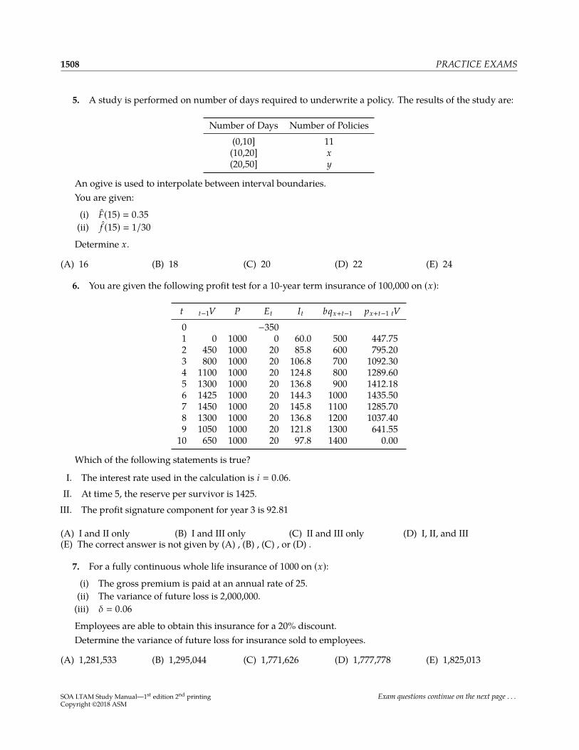
1508 PRACTICE EXAMS
5. A study is performed on number of days required to underwrite a policy. The results of the study are:
Number of Days Number of Policies(0,10] 11(10,20] x(20,50] y
An ogive is used to interpolate between interval boundaries.You are given:
(i) F(15) � 0.35(ii) f (15) � 1/30
Determine x.
(A) 16 (B) 18 (C) 20 (D) 22 (E) 24
6. You are given the following profit test for a 10-year term insurance of 100,000 on (x):
t t−1V P Et It bqx+t−1 px+t−1 tV
0 −3501 0 1000 0 60.0 500 447.752 450 1000 20 85.8 600 795.203 800 1000 20 106.8 700 1092.304 1100 1000 20 124.8 800 1289.605 1300 1000 20 136.8 900 1412.186 1425 1000 20 144.3 1000 1435.507 1450 1000 20 145.8 1100 1285.708 1300 1000 20 136.8 1200 1037.409 1050 1000 20 121.8 1300 641.55
10 650 1000 20 97.8 1400 0.00
Which of the following statements is true?
I. The interest rate used in the calculation is i � 0.06.II. At time 5, the reserve per survivor is 1425.III. The profit signature component for year 3 is 92.81
(A) I and II only (B) I and III only (C) II and III only (D) I, II, and III(E) The correct answer is not given by (A) , (B) , (C) , or (D) .
7. For a fully continuous whole life insurance of 1000 on (x):(i) The gross premium is paid at an annual rate of 25.(ii) The variance of future loss is 2,000,000.(iii) δ � 0.06
Employees are able to obtain this insurance for a 20% discount.Determine the variance of future loss for insurance sold to employees.
(A) 1,281,533 (B) 1,295,044 (C) 1,771,626 (D) 1,777,778 (E) 1,825,013
SOA LTAM Study Manual—1st edition 2nd printingCopyright ©2018 ASM
Exam questions continue on the next page . . .
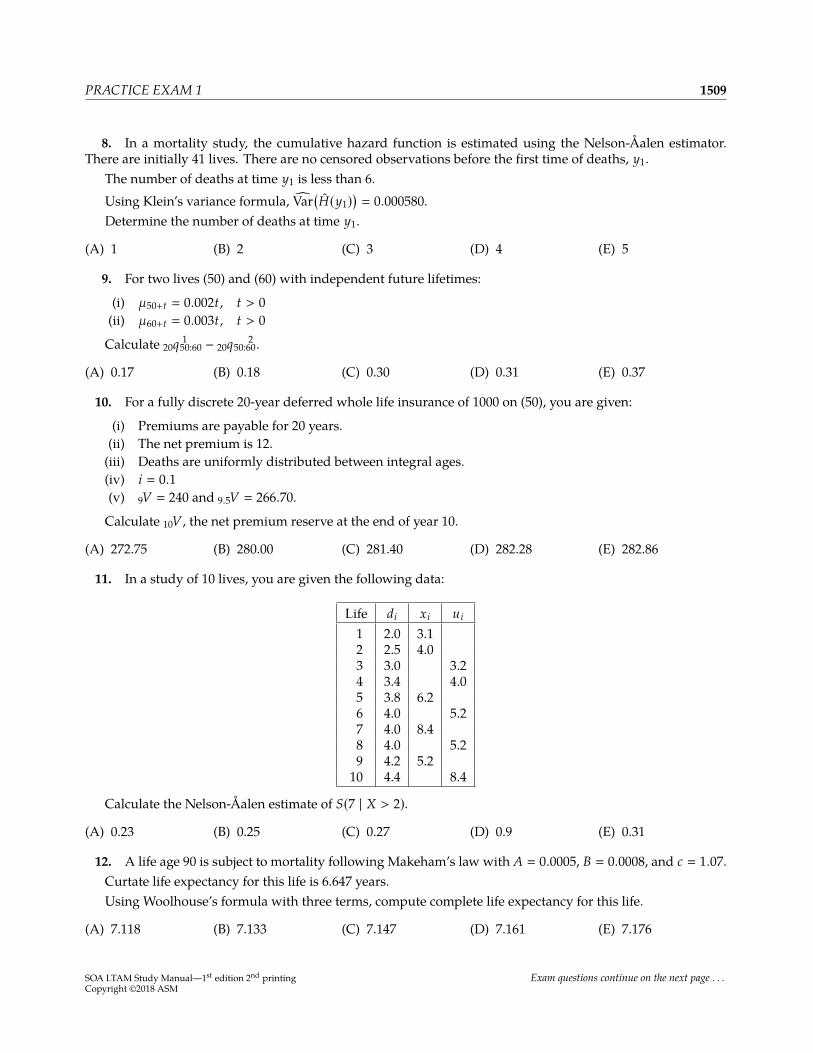
PRACTICE EXAM 1 1509
8. In a mortality study, the cumulative hazard function is estimated using the Nelson-Åalen estimator.There are initially 41 lives. There are no censored observations before the first time of deaths, y1.
The number of deaths at time y1 is less than 6.Using Klein’s variance formula, Var
(H(y1)
)� 0.000580.
Determine the number of deaths at time y1.
(A) 1 (B) 2 (C) 3 (D) 4 (E) 5
9. For two lives (50) and (60) with independent future lifetimes:
(i) µ50+t � 0.002t, t > 0(ii) µ60+t � 0.003t, t > 0
Calculate 20q501
:60 − 20q50:602 .
(A) 0.17 (B) 0.18 (C) 0.30 (D) 0.31 (E) 0.37
10. For a fully discrete 20-year deferred whole life insurance of 1000 on (50), you are given:
(i) Premiums are payable for 20 years.(ii) The net premium is 12.(iii) Deaths are uniformly distributed between integral ages.(iv) i � 0.1(v) 9V � 240 and 9.5V � 266.70.
Calculate 10V , the net premium reserve at the end of year 10.
(A) 272.75 (B) 280.00 (C) 281.40 (D) 282.28 (E) 282.86
11. In a study of 10 lives, you are given the following data:
Life di xi ui
1 2.0 3.12 2.5 4.03 3.0 3.24 3.4 4.05 3.8 6.26 4.0 5.27 4.0 8.48 4.0 5.29 4.2 5.210 4.4 8.4
Calculate the Nelson-Åalen estimate of S(7 | X > 2).(A) 0.23 (B) 0.25 (C) 0.27 (D) 0.9 (E) 0.31
12. A life age 90 is subject to mortality following Makeham’s law with A � 0.0005, B � 0.0008, and c � 1.07.Curtate life expectancy for this life is 6.647 years.Using Woolhouse’s formula with three terms, compute complete life expectancy for this life.
(A) 7.118 (B) 7.133 (C) 7.147 (D) 7.161 (E) 7.176
SOA LTAM Study Manual—1st edition 2nd printingCopyright ©2018 ASM
Exam questions continue on the next page . . .
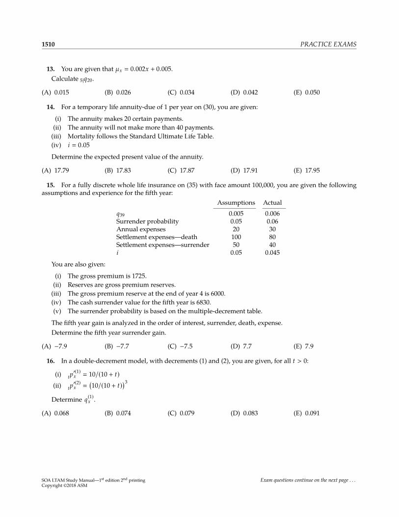
1510 PRACTICE EXAMS
13. You are given that µx � 0.002x + 0.005.Calculate 5|q20.
(A) 0.015 (B) 0.026 (C) 0.034 (D) 0.042 (E) 0.050
14. For a temporary life annuity-due of 1 per year on (30), you are given:
(i) The annuity makes 20 certain payments.(ii) The annuity will not make more than 40 payments.(iii) Mortality follows the Standard Ultimate Life Table.(iv) i � 0.05
Determine the expected present value of the annuity.
(A) 17.79 (B) 17.83 (C) 17.87 (D) 17.91 (E) 17.95
15. For a fully discrete whole life insurance on (35) with face amount 100,000, you are given the followingassumptions and experience for the fifth year:
Assumptions Actualq39 0.005 0.006Surrender probability 0.05 0.06Annual expenses 20 30Settlement expenses—death 100 80Settlement expenses—surrender 50 40i 0.05 0.045
You are also given:
(i) The gross premium is 1725.(ii) Reserves are gross premium reserves.(iii) The gross premium reserve at the end of year 4 is 6000.(iv) The cash surrender value for the fifth year is 6830.(v) The surrender probability is based on the multiple-decrement table.
The fifth year gain is analyzed in the order of interest, surrender, death, expense.Determine the fifth year surrender gain.
(A) −7.9 (B) −7.7 (C) −7.5 (D) 7.7 (E) 7.9
16. In a double-decrement model, with decrements (1) and (2), you are given, for all t > 0:
(i) tp′(1)x � 10/(10 + t)
(ii) tp′(2)x �
(10/(10 + t))3
Determine q(1)x .
(A) 0.068 (B) 0.074 (C) 0.079 (D) 0.083 (E) 0.091
SOA LTAM Study Manual—1st edition 2nd printingCopyright ©2018 ASM
Exam questions continue on the next page . . .

PRACTICE EXAM 1 1511
17. Mortality in 2015 follows the Standard Ultimate Life Table. Mortality improvement factors are
x φ(x)60 0.03261 0.03062 0.02763 0.02464 0.020
Determine the first year for which q60 is less than 0.002.
(A) 2031 (B) 2032 (C) 2033 (D) 2034 (E) 2035
18. For an insurance with face amount 100,000, you are given:(i)
ddt tV � 100
(ii) P � 1380(iii) δ � 0.05(iv) µx+t � 0.03
Determine tV .
(A) 21,000 (B) 21,500 (C) 22,000 (D) 22,500 (E) 23,000
19. In a mortality study on 5 lives, you are given the following information:
Entry age Exit age Cause of exit62.3 65.1 End of study63.5 66.0 Withdrawal64.0 65.7 Withdrawal64.2 65.5 Death64.7 67.7 End of study
Calculate the absolute difference between the actuarial estimate and the exact exposure estimate of q65.
(A) 0.002 (B) 0.006 (C) 0.010 (D) 0.014 (E) 0.018
SOA LTAM Study Manual—1st edition 2nd printingCopyright ©2018 ASM
Exam questions continue on the next page . . .
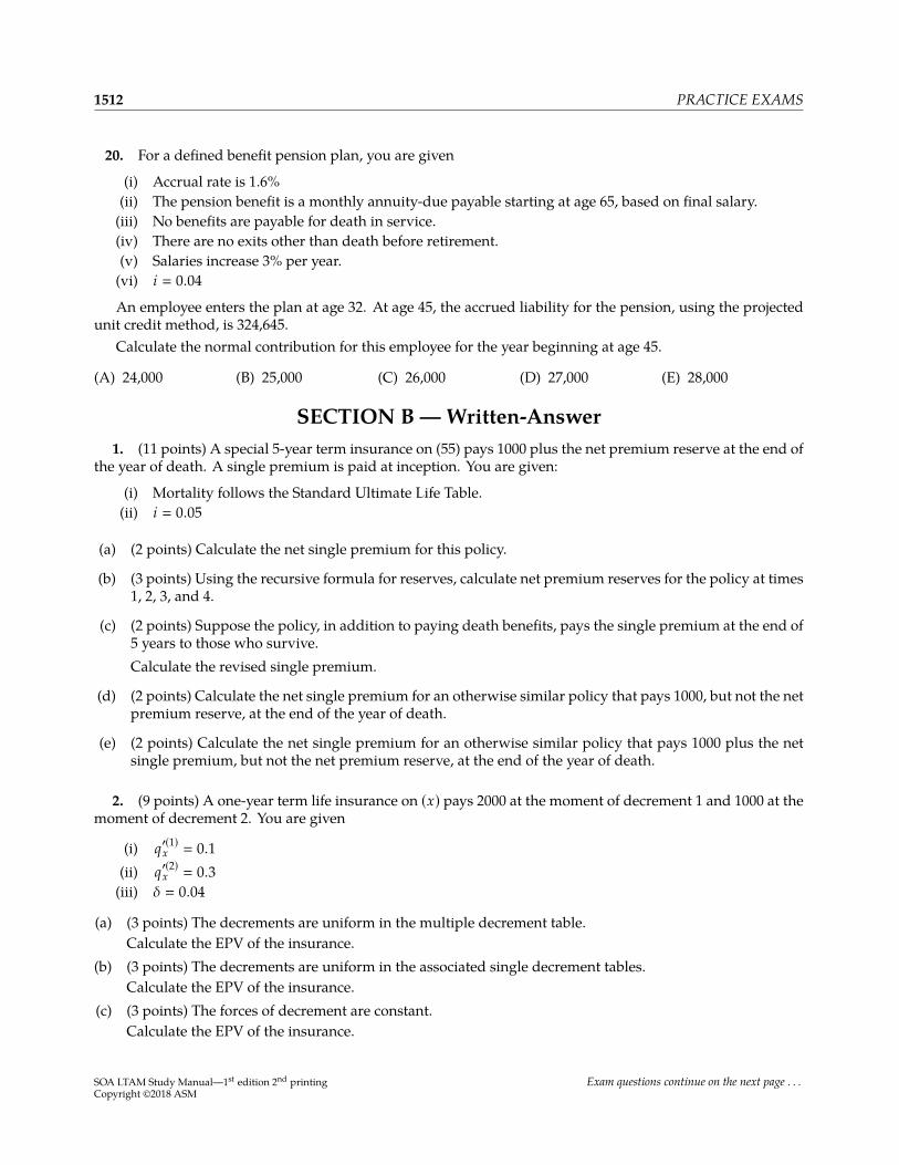
1512 PRACTICE EXAMS
20. For a defined benefit pension plan, you are given
(i) Accrual rate is 1.6%(ii) The pension benefit is a monthly annuity-due payable starting at age 65, based on final salary.(iii) No benefits are payable for death in service.(iv) There are no exits other than death before retirement.(v) Salaries increase 3% per year.(vi) i � 0.04
An employee enters the plan at age 32. At age 45, the accrued liability for the pension, using the projectedunit credit method, is 324,645.
Calculate the normal contribution for this employee for the year beginning at age 45.
(A) 24,000 (B) 25,000 (C) 26,000 (D) 27,000 (E) 28,000
SECTION B— Written-Answer1. (11 points) A special 5-year term insurance on (55) pays 1000 plus the net premium reserve at the end of
the year of death. A single premium is paid at inception. You are given:
(i) Mortality follows the Standard Ultimate Life Table.(ii) i � 0.05
(a) (2 points) Calculate the net single premium for this policy.
(b) (3 points) Using the recursive formula for reserves, calculate net premium reserves for the policy at times1, 2, 3, and 4.
(c) (2 points) Suppose the policy, in addition to paying death benefits, pays the single premium at the end of5 years to those who survive.Calculate the revised single premium.
(d) (2 points) Calculate the net single premium for an otherwise similar policy that pays 1000, but not the netpremium reserve, at the end of the year of death.
(e) (2 points) Calculate the net single premium for an otherwise similar policy that pays 1000 plus the netsingle premium, but not the net premium reserve, at the end of the year of death.
2. (9 points) A one-year term life insurance on (x) pays 2000 at the moment of decrement 1 and 1000 at themoment of decrement 2. You are given
(i) q′(1)x � 0.1(ii) q′(2)x � 0.3(iii) δ � 0.04
(a) (3 points) The decrements are uniform in the multiple decrement table.Calculate the EPV of the insurance.
(b) (3 points) The decrements are uniform in the associated single decrement tables.Calculate the EPV of the insurance.
(c) (3 points) The forces of decrement are constant.Calculate the EPV of the insurance.
SOA LTAM Study Manual—1st edition 2nd printingCopyright ©2018 ASM
Exam questions continue on the next page . . .
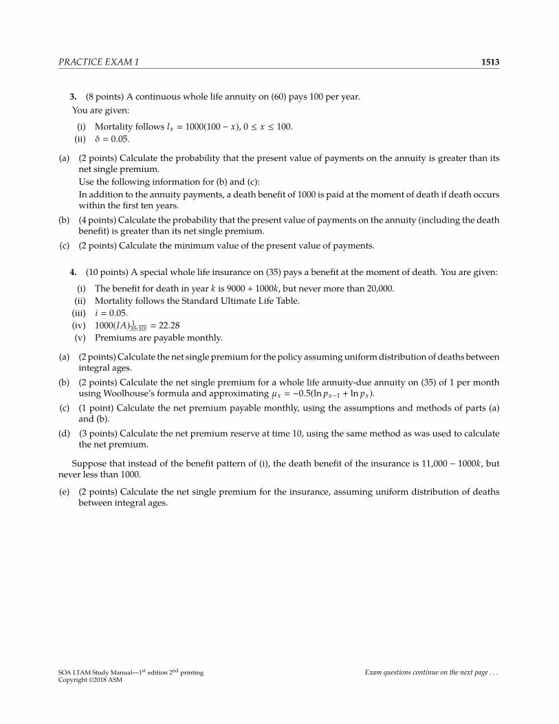
PRACTICE EXAM 1 1513
3. (8 points) A continuous whole life annuity on (60) pays 100 per year.You are given:
(i) Mortality follows lx � 1000(100 − x), 0 ≤ x ≤ 100.(ii) δ � 0.05.
(a) (2 points) Calculate the probability that the present value of payments on the annuity is greater than itsnet single premium.Use the following information for (b) and (c):In addition to the annuity payments, a death benefit of 1000 is paid at the moment of death if death occurswithin the first ten years.
(b) (4 points) Calculate the probability that the present value of payments on the annuity (including the deathbenefit) is greater than its net single premium.
(c) (2 points) Calculate the minimum value of the present value of payments.
4. (10 points) A special whole life insurance on (35) pays a benefit at the moment of death. You are given:
(i) The benefit for death in year k is 9000 + 1000k, but never more than 20,000.(ii) Mortality follows the Standard Ultimate Life Table.(iii) i � 0.05.(iv) 1000(IA)35
1:10 � 22.28
(v) Premiums are payable monthly.
(a) (2 points) Calculate the net single premium for the policy assuminguniformdistribution of deaths betweenintegral ages.
(b) (2 points) Calculate the net single premium for a whole life annuity-due annuity on (35) of 1 per monthusing Woolhouse’s formula and approximating µx � −0.5(ln px−1 + ln px).
(c) (1 point) Calculate the net premium payable monthly, using the assumptions and methods of parts (a)and (b).
(d) (3 points) Calculate the net premium reserve at time 10, using the same method as was used to calculatethe net premium.
Suppose that instead of the benefit pattern of (i), the death benefit of the insurance is 11,000 − 1000k, butnever less than 1000.
(e) (2 points) Calculate the net single premium for the insurance, assuming uniform distribution of deathsbetween integral ages.
SOA LTAM Study Manual—1st edition 2nd printingCopyright ©2018 ASM
Exam questions continue on the next page . . .

1514 PRACTICE EXAMS
5. (7 points) Your company conducts a mortality study based on policy data from Jan. 1, 2015 through Dec.31, 2016. The data for estimating q40 includes 380 policies with policyholders who were younger than age 40on Jan. 1, 2015 and older than age 40 on Dec. 31, 2016, and who neither died nor withdrew during the two-yearperiod. In addition, the data includes the following six policies:
Birth date Policy issue date Withdrawal date Death dateApr. 1, 1974 Feb. 1, 2015 — —June 1, 1974 Feb. 1, 2014 — Feb. 1, 2015Sept. 1, 1974 June 1, 2014 Aug. 1, 2015 —Jan. 1, 1975 Jan. 1, 2008 — May 1, 2015Mar. 1, 1975 Mar. 1, 2011 Dec. 1, 2016 —May 1, 1975 Dec. 1, 2005 Oct. 1, 2015 —
(a) (2 points) You use the actuarial estimator to estimate q40.Calculate the estimate.
(b) (2 points) Your boss suggests that using the Kaplan-Meier estimator would be more precise.Calculate the Kaplan-Meier estimate of q40.
(c) (2 points) Estimate the standard deviation of the Kaplan-Meier estimate of q40 usingGreenwood’s formula.(d) (1 point) Give three reasons that life insurance companies use approximations such as the actuarial
estimator to estimate mortality rates, rather than other estimation methods.
SOA LTAM Study Manual—1st edition 2nd printingCopyright ©2018 ASM
Exam questions continue on the next page . . .
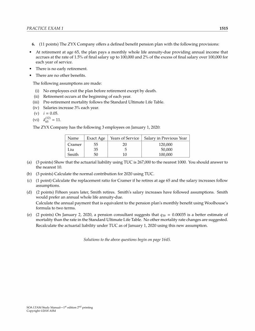
PRACTICE EXAM 1 1515
6. (11 points) The ZYX Company offers a defined benefit pension plan with the following provisions:
• At retirement at age 65, the plan pays a monthly whole life annuity-due providing annual income thataccrues at the rate of 1.5% of final salary up to 100,000 and 2% of the excess of final salary over 100,000 foreach year of service.
• There is no early retirement.• There are no other benefits.
The following assumptions are made:
(i) No employees exit the plan before retirement except by death.(ii) Retirement occurs at the beginning of each year.(iii) Pre-retirement mortality follows the Standard Ultimate Life Table.(iv) Salaries increase 3% each year.(v) i � 0.05.(vi) Üa(12)
65 � 11.
The ZYX Company has the following 3 employees on January 1, 2020:
Name Exact Age Years of Service Salary in Previous YearCramer 55 20 120,000Liu 35 5 50,000Smith 50 10 100,000
(a) (3 points) Show that the actuarial liability using TUC is 267,000 to the nearest 1000. You should answer tothe nearest 10.
(b) (3 points) Calculate the normal contribution for 2020 using TUC.(c) (1 point) Calculate the replacement ratio for Cramer if he retires at age 65 and the salary increases follow
assumptions.(d) (2 points) Fifteen years later, Smith retires. Smith’s salary increases have followed assumptions. Smith
would prefer an annual whole life annuity-due.Calculate the annual payment that is equivalent to the pension plan’s monthly benefit using Woolhouse’sformula to two terms.
(e) (2 points) On January 2, 2020, a pension consultant suggests that q39 � 0.00035 is a better estimate ofmortality than the rate in the Standard Ultimate Life Table. No other mortality rate changes are suggested.Recalculate the actuarial liability under TUC as of January 1, 2020 using this new assumption.
Solutions to the above questions begin on page 1645.
SOA LTAM Study Manual—1st edition 2nd printingCopyright ©2018 ASM
1516 PRACTICE EXAMS
SOA LTAM Study Manual—1st edition 2nd printingCopyright ©2018 ASM
Appendix A. Solutions to the Practice Exams
Answer Key for Practice Exam 11 E 6 A 11 E 16 C2 A 7 C 12 A 17 B3 C 8 A 13 D 18 B4 A 9 B 14 C 19 A5 C 10 D 15 E 20 B
Practice Exam 1
SECTION A—Multiple-Choice
1. [Section 6.2] By formula (5.2),
p60 � exp(−0.001(1.0560)
(0.05
ln 1.05
))� 0.981040
2p60 � exp(−0.001(1.0560)
(1.052 − 1ln 1.05
))� 0.961518
Then e60:2 � 0.981040 + 0.961518 � 1.9426 . (E)
2. [Lesson 15] The present value of the benefit decreases with increasing survival time, so the 95thpercentile of the present value of the insurance corresponds to the 5th percentile of survival time. The survivalprobability is
tp45 � exp(−
∫ t
00.001(1.0545+u)du
)
− ln tp45 �0.001(1.0545+u)
ln 1.05
����t
0
�0.001(1.0545+t − 1.0545)
ln 1.05Setting tp45 � 0.95,
0.001(1.0545+t − 1.0545)ln 1.05 � − ln 0.95
1.0545+t� (−1000 ln 0.95)(ln 1.05) + 1.0545
� 11.48762
1.05t�
11.487621.0545 � 1.27853
t �ln 1.27853
ln 1.05 � 5.0361
The value of Z if death occurs at t � 5.0361 is be−5.0361(0.06), so the largest face amount is 1,000,000e5.0361(0.06) �1,352,786 . (A)
SOA LTAM Study Manual—1st edition 2nd printingCopyright ©2018 ASM
1645
1646 PRACTICE EXAM 1, SOLUTIONS TO QUESTIONS A3–A5
3. [Lesson 26] The revised premium for the entire policy is 25.41 times the ratio of the revised premiumper unit at 4% to the original premium per unit at 5%.
We calculate the original net premium per unit, P601
:2 .
Üa60:2 � 1 +0.981.05 � 1.93333
A601
:2 �0.021.05 +
(0.98)(0.04)1.052 � 0.054603
P601
:2 �A60
1:2
Üa60:2�
0.0546031.93333 � 0.028243
Now we recalculate at 4%. Call the revised premium P′601
:2 .
Üa60:2 � 1 +0.981.04 � 1.94231
A601
:2 �0.021.04 +
(0.98)(0.04)1.042 � 0.055473
P′601
:2 �0.0554731.94231 � 0.028561
So the revised premium for benefit b is 25.41(0.028561/0.028243) � 25.696 . (C)
4. [Section 45.1] Let 5p010 be the probability that an entity in state 0 at time 0 transitions to state 1 before
time 5 and stays there until time 5, and let 5p105 be the probability that an entity in state 1 at time 5 transitions
to state 0 before time 10 and stays there until time 10. We’ll use formula (45.9) for both transitions. Notice thatthe formula is the same with 0 and 1 switched, except that 5p01
0 uses µ01 � 0.05 and 5p105 uses µ10 � 0.04 outside
the parentheses.
e−µ0•t
µ1• − µ0• +e−µ1•t
µ0• − µ1• �e−0.08(5)
0.14 − 0.08 +e−0.14(5)
0.08 − 0.14 � 2.89558
5p010 � 0.05(2.89558) � 0.14478
5p105 � 0.04(2.89558) � 0.11582
The answer is (0.14478)(0.11582) � 0.01677 . (A)
5. [Section 64.2]
F(15) � 11 + 0.5x11 + x + y
� 0.35
f (15) � x10(11 + x + y) � 1/30
Multiply the second equation by 10.f (15) � x
11 + x + y� 1/3
Divide it into the F(15) equation.11 + 0.5x
x� 1.05
11 + 0.5x � 1.05x11 � 0.55x
x � 20 (C)
SOA LTAM Study Manual—1st edition 2nd printingCopyright ©2018 ASM
PRACTICE EXAM 1, SOLUTIONS TO QUESTIONS A6–A9 1647
6. [Lesson 73]I From the row for year 1, with 0 reserves and expenses, we see that It/Pt � 0.06, so the interest rate is
0.06.!II Looking at the line for t � 6, we see that the reserve per survivor to time t − 1 � 5 is 1425. !
III First, the profit in year 3 is 800 + 1000 − 20 + 106.8 − 700 − 1092.3 � 94.50. We deduce survivorship fromthe bqx+t−1 column, and we see that the mortality rates in the first two years are 0.005 and 0.006, so theprofit signature component of year‘3 is (0.995)(0.994)(94.50) � 93.46. #.
(A)
7. [Lesson 32] The variance of future loss for a gross premium of 25 is
2,000,000 � Var(vTx
) (1000 +
250.06
)2
� Var(vTx
) (2,006,944)If we replace 25 with 20 (for a 20% discount) in the above formula, it becomes
Var (0L) � Var(vTx
) (1000 +
200.06
)2
� Var(vTx
) (1,777,778)We see that this is 1,777,778/2,006,944 times the given variance, so the final answer is
Var(0L) � 1,777,7782,006,944 (2,000,000) � 1,771,626 (C)
8. [Section 68.1]
s1(41 − s1)413 � 0.00058
s1(41 − s1) � 40
s1 � 1 , 40 (A)
9. [Lesson 58] 20q501
:60 − 20q50:602� 20q50 20p60, and
20q50 � 1 − exp(−
∫ 20
00.002t dt
)
� 1 − e−0.001(20)2� 1 − 0.670320 � 0.329680
20p60 � exp(−
∫ 20
00.003t dt
)
� e−0.0015(20)2� 0.548812
20q50 20p60 � (0.329680)(0.548812) � 0.180932 (B)
SOA LTAM Study Manual—1st edition 2nd printingCopyright ©2018 ASM

1648 PRACTICE EXAM 1, SOLUTIONS TO QUESTIONS A10–A13
10. [Section 42.2] We need to back out q59. We use reserve recursion. Since the insurance is deferred,1000q59 is not subtracted from the left side.
(9V + P)(1.10.5) � 9.5V(1 − 0.5q59)252(1.10.5) � 266.70 − 133.35q59
q59 �2.40017133.35 � 0.018
Then the net premium reserve at time 10 is, by recursion from time 9,
252(1.1)1 − 0.018 � 282.28 (D)
11. [Lesson 66] Risk sets are:At time 3.1, lives 1,2,3At time 4.0, lives 2,4,5At time 5.2, lives 5–10At time 6.2, lives 5,7,10
yi ri si H(7 | X ≥ 2)3.1 3 1 1/34.0 3 1 2/35.2 6 1 5/66.2 3 1 7/6
S(7 | X > 2) � e−7/6� 0.3114 (E)
12. [Section 24.2] By equation (24.10),
ex � ex +12 − 1
12µx
Force of mortality for (90) is µ90 � 0.0005 + 0.0008(1.0790) � 0.353382. Thus
e90 � 6.647 + 0.5 − 112 (0.353382) � 7.118 (A)
13. [Lesson 4] 5|q20 �(S0(25)−S0(26)) /S0(20), sowewill calculate these three values of S0(x). (Equivalently,
one could calculate 5p20 and 6p20 and take the difference.) The integral of µx is∫ x
0µu du �
(0.002u2
2 + 0.005u)����
x
0� 0.001x2
+ 0.005x
so
S0(20) � exp(−(0.001(202) + 0.005(20)) ) � exp(−0.5) � 0.606531
S0(25) � exp(−(0.001(252) + 0.005(25)) ) � exp(−0.75) � 0.472367
S0(26) � exp(−(0.001(262) + 0.005(26)) ) � exp(−0.806) � 0.446641
and the answer is5|q20 �
0.472367 − 0.4466410.606531 � 0.042415 (D)
SOA LTAM Study Manual—1st edition 2nd printingCopyright ©2018 ASM
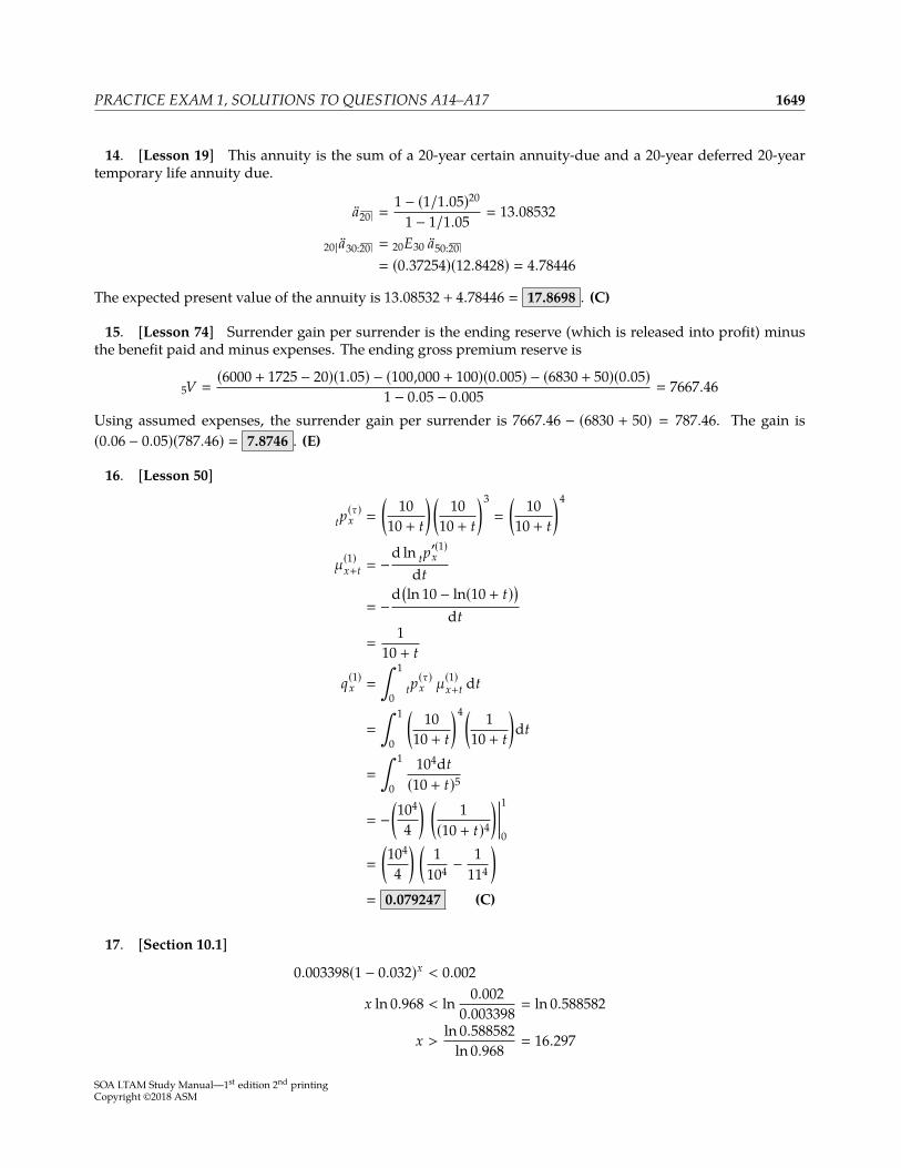
PRACTICE EXAM 1, SOLUTIONS TO QUESTIONS A14–A17 1649
14. [Lesson 19] This annuity is the sum of a 20-year certain annuity-due and a 20-year deferred 20-yeartemporary life annuity due.
Üa20 �1 − (1/1.05)20
1 − 1/1.05� 13.08532
20| Üa30:20 � 20E30 Üa50:20� (0.37254)(12.8428) � 4.78446
The expected present value of the annuity is 13.08532 + 4.78446 � 17.8698 . (C)
15. [Lesson 74] Surrender gain per surrender is the ending reserve (which is released into profit) minusthe benefit paid and minus expenses. The ending gross premium reserve is
5V �(6000 + 1725 − 20)(1.05) − (100,000 + 100)(0.005) − (6830 + 50)(0.05)
1 − 0.05 − 0.005 � 7667.46
Using assumed expenses, the surrender gain per surrender is 7667.46 − (6830 + 50) � 787.46. The gain is(0.06 − 0.05)(787.46) � 7.8746 . (E)
16. [Lesson 50]
tp(τ)x �
(10
10 + t
) (10
10 + t
)3
�
(10
10 + t
)4
µ(1)x+t � −d ln tp
′(1)x
dt
� −d(ln 10 − ln(10 + t))
dt
�1
10 + t
q(1)x �
∫ 1
0tp(τ)x µ(1)x+t dt
�
∫ 1
0
(10
10 + t
)4 ( 110 + t
)dt
�
∫ 1
0
104dt(10 + t)5
� −(104
4
) (1
(10 + t)4)����
1
0
�
(104
4
) (1
104 −1
114
)
� 0.079247 (C)
17. [Section 10.1]
0.003398(1 − 0.032)x < 0.002
x ln 0.968 < ln 0.0020.003398 � ln 0.588582
x >ln 0.588582
ln 0.968 � 16.297
SOA LTAM Study Manual—1st edition 2nd printingCopyright ©2018 ASM
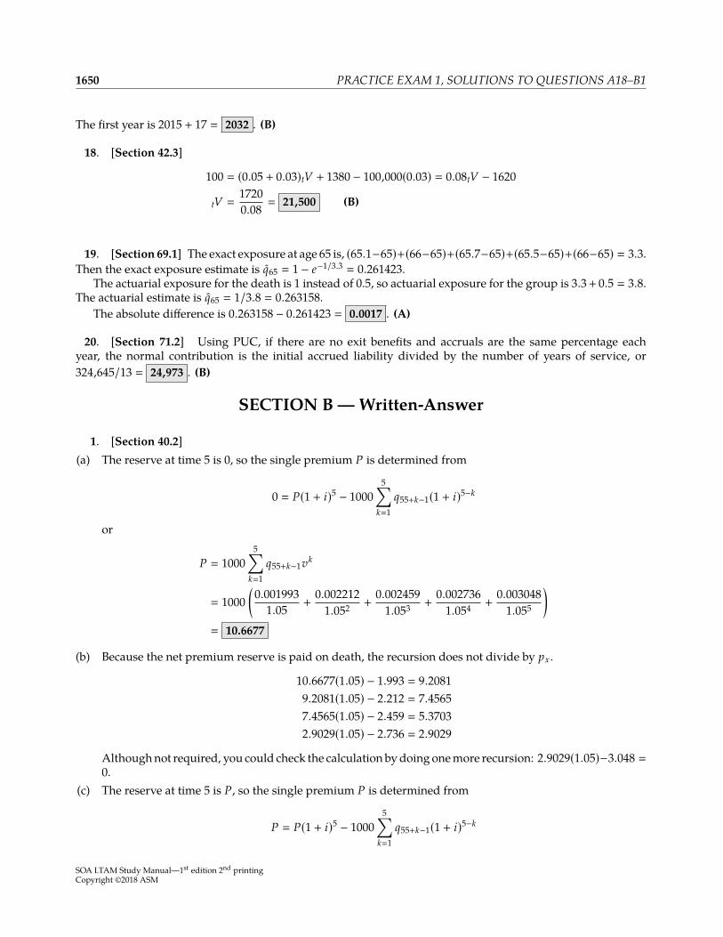
1650 PRACTICE EXAM 1, SOLUTIONS TO QUESTIONS A18–B1
The first year is 2015 + 17 � 2032 . (B)
18. [Section 42.3]
100 � (0.05 + 0.03)tV + 1380 − 100,000(0.03) � 0.08tV − 1620
tV �17200.08 � 21,500 (B)
19. [Section 69.1] The exact exposure at age 65 is, (65.1−65)+(66−65)+(65.7−65)+(65.5−65)+(66−65) � 3.3.Then the exact exposure estimate is q65 � 1 − e−1/3.3 � 0.261423.
The actuarial exposure for the death is 1 instead of 0.5, so actuarial exposure for the group is 3.3+ 0.5 � 3.8.The actuarial estimate is q65 � 1/3.8 � 0.263158.
The absolute difference is 0.263158 − 0.261423 � 0.0017 . (A)
20. [Section 71.2] Using PUC, if there are no exit benefits and accruals are the same percentage eachyear, the normal contribution is the initial accrued liability divided by the number of years of service, or324,645/13 � 24,973 . (B)
SECTION B— Written-Answer
1. [Section 40.2](a) The reserve at time 5 is 0, so the single premium P is determined from
0 � P(1 + i)5 − 10005∑
k�1q55+k−1(1 + i)5−k
or
P � 10005∑
k�1q55+k−1vk
� 1000(
0.0019931.05 +
0.0022121.052 +
0.0024591.053 +
0.0027361.054 +
0.0030481.055
)
� 10.6677
(b) Because the net premium reserve is paid on death, the recursion does not divide by px .
10.6677(1.05) − 1.993 � 9.20819.2081(1.05) − 2.212 � 7.45657.4565(1.05) − 2.459 � 5.37032.9029(1.05) − 2.736 � 2.9029
Althoughnot required, you could check the calculation bydoing onemore recursion: 2.9029(1.05)−3.048 �
0.(c) The reserve at time 5 is P, so the single premium P is determined from
P � P(1 + i)5 − 10005∑
k�1q55+k−1(1 + i)5−k
SOA LTAM Study Manual—1st edition 2nd printingCopyright ©2018 ASM
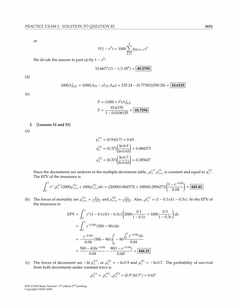
PRACTICE EXAM 1, SOLUTION TO QUESTION B2 1651
or
P(1 − v5) � 10005∑
k�1q55+k−1vk
We divide the answer to part (a) by 1 − v5:
10.6677/(1 − 1/1.055) � 49.2795
(d)
1000A551
:5 � 1000(A55 − 5E55 A60) � 235.24 − (0.77382)(290.28) � 10.6155
(e)
P � (1000 + P)A551
:5
P �10.6155
1 − 0.0106155 � 10.7294
2. [Lessons 51 and 53](a)
p(τ)x � (0.9)(0.7) � 0.63
q(1)x � (0.37)(
ln 0.9ln 0.63
)� 0.084373
q(2)x � (0.37)(
ln 0.7ln 0.63
)� 0.285627
Since the decrements are uniform in the multiple decrement table, sp(τ)x µ
( j)x+s is constant and equal to q( j)x .
The EPV of the insurance is∫ 1
0vs
sp(τ)x (2000µ(1)x+s + 1000µ(2)x+s)ds �
(2000(0.084373) + 1000(0.285627)) (1 − e−0.04
0.04
)� 445.41
(b) The forces of mortality are µ(1)x+s �0.1
1−0.1s and µ(2)x+s �0.3
1−0.3s . Also, sp(τ)x � (1 − 0.1s)(1 − 0.3s). So the EPV of
the insurance is
EPV �
∫ 1
0vs(1 − 0.1s)(1 − 0.3s)
(2000 0.1
1 − 0.1s+ 1000 0.3
1 − 0.3s
)ds
�
∫ 1
0e−0.04s(500 − 90s)ds
� − e−0.04s
0.04 (500 − 90s)����1
0− 90
∫ 10 e−0.04sds
0.04
�500 − 410e−0.04
0.04 − 90(1 − e−0.04)0.042 � 446.31
(c) The forces of decrement are − ln p′( j)x , or µ(1)x � − ln 0.9 and µ(2)x � − ln 0.7. The probability of survivalfrom both decrements under constant force is
sp(τ)x � sp
′(1)x , sp
′(2)x � (0.9s)(0.7s) � 0.63s
SOA LTAM Study Manual—1st edition 2nd printingCopyright ©2018 ASM

1652 PRACTICE EXAM 1, SOLUTION TO QUESTION B3
The EPV of the insurance is
EPV �
∫ 1
0vs
sp(τ)x (2000µ(1)x + 1000µ(2)x )ds
�
∫ 1
0e(−0.04+ln 0.63)s(−2000 ln 0.9 − 1000 ln 0.7︸ ︷︷ ︸
567.396
)ds
� 567.396∫ 1
0e(−0.04+ln 0.63)sds
�567.396
− ln 0.63 + 0.04 (1 − 0.63e−0.04) � 446.09
3. [Lesson 22](a) First let’s calculate the net single premium. We can ignore the 100 per year factor; it just scales up the
numbers.
A60 �1 − e−0.05(40)
0.05(40) � 0.432332
a60 �1 − 0.432332
0.05 � 11.35335
aT � a60 when:
1 − e−0.05t
0.05 �1 − 0.432332
0.05e−0.05t
� 0.432332
t � − ln 0.4323320.05 � 16.77121
The probability that T60 > 16.77121 is 1 − 16.77121/40 � 0.58072 .(b) First let’s calculate the net single premium.
A601
:10 �1 − e−0.05(10)
0.05(40) � 0.196735
1000A601
:10 + 100 Üa60 � 196.735 + 1135.335 � 1332.070
The present value of payments may be higher than 1332.070 in the first 10 years. However, let’s begin bycalculating the time t > 10 at which the present value of payments is higher than 1332.070.
100(1 − e−0.05t
0.05
)� 1332.070
e−0.05t� 0.333965
t � − ln 0.3339650.05 � 21.93438
Now let’s determine the time t < 10 for which the present value of payments is 1332.070.
1000e−0.05t+ 100
(1 − e−0.05t
0.05
)� 1332.07
SOA LTAM Study Manual—1st edition 2nd printingCopyright ©2018 ASM
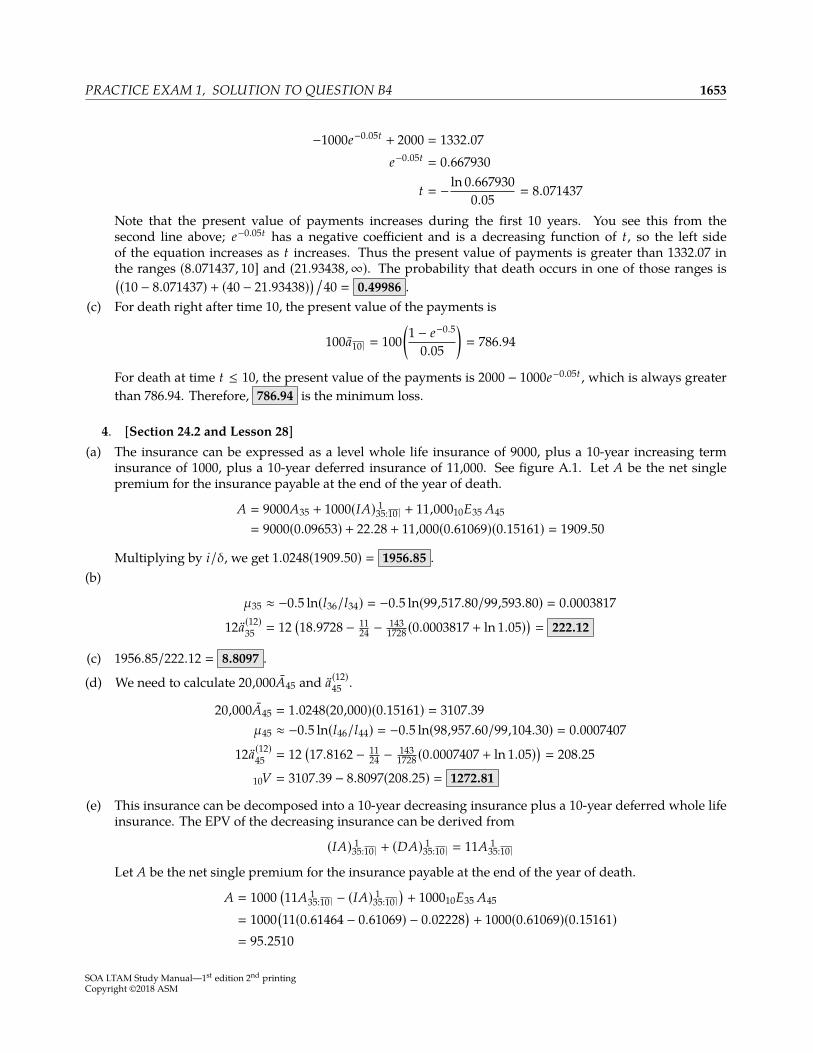
PRACTICE EXAM 1, SOLUTION TO QUESTION B4 1653
−1000e−0.05t+ 2000 � 1332.07e−0.05t
� 0.667930
t � − ln 0.6679300.05 � 8.071437
Note that the present value of payments increases during the first 10 years. You see this from thesecond line above; e−0.05t has a negative coefficient and is a decreasing function of t, so the left sideof the equation increases as t increases. Thus the present value of payments is greater than 1332.07 inthe ranges (8.071437, 10] and (21.93438,∞). The probability that death occurs in one of those ranges is((10 − 8.071437) + (40 − 21.93438)) /40 � 0.49986 .
(c) For death right after time 10, the present value of the payments is
100a10 � 100(1 − e−0.5
0.05
)� 786.94
For death at time t ≤ 10, the present value of the payments is 2000 − 1000e−0.05t , which is always greaterthan 786.94. Therefore, 786.94 is the minimum loss.
4. [Section 24.2 and Lesson 28](a) The insurance can be expressed as a level whole life insurance of 9000, plus a 10-year increasing term
insurance of 1000, plus a 10-year deferred insurance of 11,000. See figure A.1. Let A be the net singlepremium for the insurance payable at the end of the year of death.
A � 9000A35 + 1000(IA)351
:10 + 11,00010E35 A45
� 9000(0.09653) + 22.28 + 11,000(0.61069)(0.15161) � 1909.50
Multiplying by i/δ, we get 1.0248(1909.50) � 1956.85 .(b)
µ35 ≈ −0.5 ln(l36/l34) � −0.5 ln(99,517.80/99,593.80) � 0.0003817
12 Üa(12)35 � 12
(18.9728 − 11
24 − 1431728 (0.0003817 + ln 1.05)) � 222.12
(c) 1956.85/222.12 � 8.8097 .
(d) We need to calculate 20,000A45 and Üa(12)45 .
20,000A45 � 1.0248(20,000)(0.15161) � 3107.39µ45 ≈ −0.5 ln(l46/l44) � −0.5 ln(98,957.60/99,104.30) � 0.0007407
12 Üa(12)45 � 12
(17.8162 − 11
24 − 1431728 (0.0007407 + ln 1.05)) � 208.25
10V � 3107.39 − 8.8097(208.25) � 1272.81
(e) This insurance can be decomposed into a 10-year decreasing insurance plus a 10-year deferred whole lifeinsurance. The EPV of the decreasing insurance can be derived from
(IA)351
:10 + (DA)351
:10 � 11A351
:10
Let A be the net single premium for the insurance payable at the end of the year of death.
A � 1000(11A35
1:10 − (IA)35
1:10
)+ 100010E35 A45
� 1000(11(0.61464 − 0.61069) − 0.02228
)+ 1000(0.61069)(0.15161)
� 95.2510
SOA LTAM Study Manual—1st edition 2nd printingCopyright ©2018 ASM
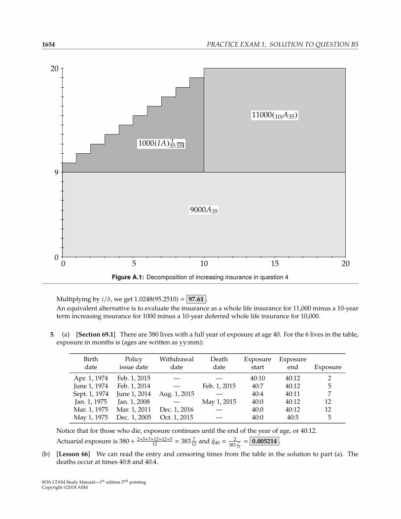
1654 PRACTICE EXAM 1, SOLUTION TO QUESTION B5
11000(10|A35)
1000(IA)351
:10
9000A35
0 5 10 15 20
9
0
20
Figure A.1: Decomposition of increasing insurance in question 4
Multiplying by i/δ, we get 1.0248(95.2510) � 97.61 .An equivalent alternative is to evaluate the insurance as a whole life insurance for 11,000 minus a 10-yearterm increasing insurance for 1000 minus a 10-year deferred whole life insurance for 10,000.
5. (a) [Section 69.1] There are 380 lives with a full year of exposure at age 40. For the 6 lives in the table,exposure in months is (ages are written as yy:mm):
Birth Policy Withdrawal Death Exposure Exposuredate issue date date date start end Exposure
Apr. 1, 1974 Feb. 1, 2015 — — 40:10 40:12 2June 1, 1974 Feb. 1, 2014 — Feb. 1, 2015 40:7 40:12 5Sept. 1, 1974 June 1, 2014 Aug. 1, 2015 — 40:4 40:11 7Jan. 1, 1975 Jan. 1, 2008 — May 1, 2015 40:0 40:12 12Mar. 1, 1975 Mar. 1, 2011 Dec. 1, 2016 — 40:0 40:12 12May 1, 1975 Dec. 1, 2005 Oct. 1, 2015 — 40:0 40:5 5
Notice that for those who die, exposure continues until the end of the year of age, or 40:12.Actuarial exposure is 380 +
2+5+7+12+12+512 � 383 7
12 and q40 �2
383 712
� 0.005214 .
(b) [Lesson 66] We can read the entry and censoring times from the table in the solution to part (a). Thedeaths occur at times 40:8 and 40:4.
SOA LTAM Study Manual—1st edition 2nd printingCopyright ©2018 ASM
PRACTICE EXAM 1, SOLUTION TO QUESTION B6 1655
yi ri si
40:4 383 140:8 383 1
The Kaplan Meier estimate is
q40 � 1 −(1 − 1
383
) (1 − 1
383
)� 0.005115
(c) [Section 68.1] Using Greenwood’s formula,
(1 − 0.005115)√
1(383)(382) +
1(383)(382) � 0.003678
(d) [Lesson 69](a) No parametric distribution provides an adequate model.(b) Values of the survival function are only required at integers.(c) There is a large volume of data, almost all truncated or censored.
6. [Lesson 71](a) For Cramer, 10E55 � 0.59342.
20(0.015(100,000) + 0.02(20,000))(0.59342)(11) � 248,049.6
For Liu, 30E35 � (0.61069)(0.35994) � 0.21981.
5((0.015)(50,000))(0.21981)(11) � 9,067.2
For Smith, 15E50 � (0.77772)(0.59342) � 0.46151.
10(0.015)(100,000)(0.46151)(11) � 76,149.9
Total actuarial liability is 248,049.6 + 9,067.2 + 76,149.9 � 333,267 .(b) For Cramer, salary will be 120, 000(1.03) � 123,600 next year. The discounted value of next year’s liability
is21
(0.015(100,000) + 0.02(23,600))(0.59342)(11) � 270,321.8
For Liu, salary will not exceed 100,000, so we can calculate the normal contribution directly using for-mula (71.2):
9,067.2(1.03
(65
)− 1
)� 2,139.9
For Smith, salary will be 100,000(1.03) � 103,000 next year. The discounted value of next year’s liability is
11(0.015(100,000) + 0.02(3,000))(0.59342)(11) � 87,115.5
The normal contribution is (270,321.8 − 248,049.6) + 2,139.9 + (87,115.5 − 76,149.9) � 33,238 .
(c) Final salary is 120,000(1.0310) � 161,270. Annual pension is
30(0.015(100,000) + 0.02(61,270)) � 81,762
The replacement ratio is 81,762/161,270 � 0.5070 .
SOA LTAM Study Manual—1st edition 2nd printingCopyright ©2018 ASM
1656 PRACTICE EXAM 1, SOLUTION TO QUESTION B6
(d) Final salary is 100,000(1.0315) � 155,797. The annual payment under a monthly annuity-due is
25(0.015(100,000) + 0.02(55,797)) � 65,398
By Woolhouse’s formula to two terms, Üa(12)65 � Üa65 − 11
24 , so Üa65 � 11 1124 , and
63,130 Üa(12)65 � x Üa65
x � 65,398(
1111 11
24
)� 62,782
(e) This change only affects Liu. We must recalculate 30E35 for Liu. We’ll calculate it from first principles,although you may also calculate 5E35 and then multiply by 25E40 which can be calculated from the pureendowment columns of the Standard Ultimate Life Table.
30p35 � 4p35 p39 25p40
�
(99,387.3099,556.70
)(1 − 0.00035)
(94,579.7099,338.30
)� 0.950144
30E35 �0.950144
1.0530 � 0.21984
The revised liability for Liu is
5((0.015)(50,000))(0.21984)(11) � 9068.5
instead of the previous 9067.2 calculated in part (a). The actuarial liability increases by 1 and becomes333,268 .
SOA LTAM Study Manual—1st edition 2nd printingCopyright ©2018 ASM
Related Documents