Snow water equivalent time-series forecasting in Ontario, Canada, in link to large atmospheric circulations

HYDROLOGICAL PROCESSESHydrol. Process. (2014)Published online in Wiley Online Library(wileyonlinelibrary.com) DOI: 10.1002/hyp.10184

Snow water equivalent time-series forecasting in Ontario,Canada, in link to large atmospheric circulations

Ali Sarhadi,1* Richard Kelly2 and Reza Modarres31 Department of Civil and Environmental Engineering, University of Waterloo, Waterloo, Ontario, Canada, N2L-3G1

2 Department of Geography and Environmental Management, University of Waterloo, Waterloo, Ontario, Canada, N2L-3G13 Institute National de la Recherche Scientifique, 490 rue de la couronne, Québec, Québec, Canada, G1K 9A9

*CEnE-m

Co

Abstract:

The present study applies different time-series models for forecasting daily and monthly snow water equivalent (SWE) data inOntario, Canada, during 1987–2011. For daily time series, which showed a significant negative trend, four categories of theautoregressive moving-average (ARMA) and ARMA model with exogenous variables (ARMAX) were applied. The NorthAtlantic Oscillation, Southern Oscillation Index and Pacific/North American Pattern, as large-scale atmospheric anomalies, aswell as temperature time series are considered as exogenous variables for ARMAX models. According to the multicriteriaperformance evaluation, a time-trend ARMAX model demonstrated the best performance for modelling and forecasting dailySWE. Two models, seasonal autoregressive integrated moving average (SARIMA) and SARIMA with exogenous variables(SARIMAX), were also fitted to the monthly SWE time series. The results revealed that the SARIMAX model showed a betterperformance than the SARIMA model according to multicriteria evaluation. The three nonparametric tests, Wilcoxon, Leveneand Kolmogorov–Smirnov for forecasting evaluation demonstrated that the selected time-series models had enough reliability forshort-term SWE forecasting in Ontario. The results of this study also demonstrate the importance of incorporating both trend andappropriate exogenous variables for SWE time-series modelling and forecasting. Copyright © 2014 John Wiley & Sons, Ltd.

KEY WORDS time-series forecasting; snow water equivalent; time-trend ARMAX; SARIMAX; Ontario

Received 26 June 2013; Accepted 24 February 2014

INTRODUCTION

Snowmelt runoff is considered as one of the main sourcesof surface water supply in mid-latitude to high-latituderiver catchments and has a key role in regional-scalewater resources management (McNamara et al., 1998;Dery et al., 2005). From a hydrological point of view,snow water equivalent (SWE) is the total water stored in asnowpack that is available when the pack melts.Therefore, SWE forecasting can help water resourcesauthorities define accurate water operating policies foreffective water management, such as reservoir flowregulation, agricultural surface water allocation andhydropower generation scheduling. Hence, the accuracyof SWE forecasting has a significant effect on theoperation efficiency of the water resources systems(Karamouz and Zahraie, 2004).In the past decades, many researchers have developed

statistical methods to model behaviour of hydroclimatictime series affected by stochastic periodic components.

orrespondence to: Ali Sarhadi, Department of Civil and Environmentalgineering, University ofWaterloo,Waterloo, Ontario, Canada N2L-3G1.ail: [email protected]

pyright © 2014 John Wiley & Sons, Ltd.

Autoregressive moving-average (ARMA) time-seriesmodels developed by Box and Jenkins (1976) have beena common approach among hydrologists for modellingand forecasting time-varying statistical characteristics ofhydroclimate variables (Salas et al., 1980; Hipel andMcLeod, 1994). Different studies have used the ARMAmodel and its extensions, such as autoregressive integrat-ed moving-average (ARIMA), seasonal ARIMA(SARIMA) and ARMA with exogenous variable(ARMAX) models, for modelling and forecasting hydro-logical and climatological variables such as precipitation(Soltani et al., 2007), drought (Mishra and Desai, 2005)and stream flow (Modarres, 2007). However, very fewapplications of ARMA models have been developed forSWE modelling and forecasting. For example, Haltinerand Salas (1988) used ARMAX for forecasting dailystream flow resulting from snowmelt and rainfall in theRio Grande River in southern Colorado and reportedimproved flow forecasts with fewer model parameters.However, the emphasis in this study was on stream flowforecasting and not on SWE prediction.The aim of this study is to develop different types of

ARMA models for daily and monthly SWE time-seriesforecasting in Ontario. In addition, the present study

A. SARHADI, R. KELLY AND R. MODARRES

attempts to develop ARMAX models with exogenousvariables such as a number of large-scale atmosphericlow-frequency variability modes and local observedmeteorological data, for SWE time-series forecasting.The next section provides the proposedmethods for SWE

time-series forecasting. The methods are followed by anillustrative example of 24 years of daily and monthlysatellite-based SWE time-series modelling for Ontario,Canada. The results section presents the key findings, andthe last section discusses the significance of the results,concluding with recommendations for future studies.

METHODOLOGY

Time-series models

To analyse stochastic characteristics of the hydroclimatictime series, the general time-series model is described by amultiplicative SARIMA(p, d, q) × (P, D, Q)s model, whichis shown in the following form:

ϕp Bð ÞΦP BS� �

∇d∇SDYt ¼ θq Bð ÞΘQ BS

� �at (1)

where Yt is the observed time series, ϕp(B) is a polynomialof order p, θq(B) is a polynomial of order q, ∇d is thenonseasonal differencing operator, B is the backwardoperator, ΦP and ΘQ are the seasonal polynomials of ordersP andQ,∇D

S is the seasonal differencing operators, S representsthe seasons and at is an independent identically distributednormal error with a zero mean and standard deviation σa.The following equations give the nonseasonal and

seasonal differencing operators, which are selected to bejust large enough to remove all nonseasonal and seasonalnonstationarity:

∇dYt ¼ 1� Bð ÞdYt and BdYt ¼ Yt�d (2)

∇SDYt ¼ 1� BS

� �Yt and BDYt ¼ Yt�D (3)

In the multiplicative form of the SARIMA model, thenonseasonal and seasonal autoregressive operators aremultiplied together on the left-hand side while themoving-average operators are multiplied together on theright-hand side (Hipel and McLeod, 1994).The preceding model is applied in the case of existing

seasonality (or significant autocorrelation coefficients athigher seasonal lag times, k = 12, 24, 36, …). If noseasonality is observed in Yt, the preceding model reducesto the following ARIMA model:

ϕp Bð Þ∇dYt ¼ θq Bð Þat (4)

For those time series that do not show a nonseasonalnonstationarity (or significant autocorrelation coefficients

Copyright © 2014 John Wiley & Sons, Ltd.

at higher lag times, k> 7), the ARIMA model will reduceto an ARMA model, which contains two polynomials oforder p and q, as is shown in the following:

ϕp Bð ÞYt ¼ θq Bð Þat (5)

The preceding ARIMA and SARIMA models can beused to model a single time series. However, in somesituations, we need to predict a hydroclimatic variable byusing a number of predictors called ‘exogenous variables’through time. This type of model is called an ARMAXmodel, which can be written as

ϕp Bð ÞYt ¼ ωs Bð Þxt þ θq Bð Þat (6)

where ωs is the parameter of the model and x is theindependent variable. This type of model is used in thisstudy for modelling the temporal relationship betweenan SWE (as an independent variable) and exogenousvariables.

Time-series modelling procedure

To establish time-series models, three steps should befollowed: model identification, parameter estimation andgoodness-of-fit test. These three steps are described brieflyin the following sections (Hipel and McLeod, 1994).

Model identification. The purpose of the identificationstep is to represent the behaviour of the time series, and todetermine if the series is nonseasonal or seasonal andthe order of both seasonal and nonseasonal parameters(P, Q, p and q).To identify the order of the model, the autocorrelation

function (ACF) and partial ACF (PACF) are used, both ofwhich measure the amount of a linear dependence amongobservations separated by k time lags and residuals oftime series. The presence of nonstationarity in the seriesand a cyclic behaviour produced by seasonality can bevirtually detected using ACF and PACF. If the autocor-relation coefficients are significant for large lag times(usually k> 7–10), the series is assumed nonstationary intime. On the other hand, if the autocorrelation coefficientsare significant at lags k = 12, 24, 36, …, it is said that thetime series has a seasonal variation and nonstationary. Anonseasonal or seasonal differencing operator is used toconvert a nonstationary series to a stationary time series.

Model estimation. The next step after identifying aninitial model in the first step is the efficient estimation ofthe model’s parameters. The parameters should satisfytwo conditions, stationarity and invertibility, for theautoregressive and moving-average models (Box andJenkins, 1976; Salas et al., 1980). The parameters that are

Hydrol. Process. (2014)

SNOW WATER EQUIVALENT TIME-SERIES FORECASTING

estimated by statistical methods such as the method ofmoments or the method of maximum likelihood shouldalso be statistically significant. If the model’s parameterssatisfy the preceding conditions, they are kept in themodel, and the model’s adequacy is then checked in thenext step. Otherwise, the order of the initial candidatemodel should be changed, and its parameters shouldsatisfy the adequate order of parameters and theirsignificant estimates.

Model diagnostic checking. Model diagnostic checkingor goodness-of-fit testing includes testing for autocorre-lation in the residuals of the model. In other words, amodel should have time independent and normallydistributed residuals to be considered adequate. In thisstudy, two methods are applied to test the nonexistence oftime independence in the structure of the model residuals.A simple method is an inspection of the ACF of theresiduals (or PACF). The lag k autocorrelation co-efficients of the residuals of an independent series oflength of n are assumed to be normally distributed with amean of zero and a variance of 1/n. The 95% confidencelimits are given by ±1.96/√n. The validity of a time-series model is accepted if all autocorrelation coefficientsfall within the confidence limit.The other common test used to test time independence

and normality of the residuals is the Ljung–Box lack-of-fit test (Box and Jenkins, 1976). This test, more formally,the Portmanteau lack-of-fit test, computes a statistic, Q,which is approximately distributed as χ2(L� p� q) and isgiven by

Q ¼ N N þ 2ð Þ∏Li¼1 N � kð Þ�1r2k εð Þ (7)

where N is the sample size and L is the number ofautocorrelations of the residuals included in the statistic. Lcan vary between 15 and 25 for nonseasonal models and 2Sand 4S for seasonal models (Hipel andMcLeod, 1994). rk isthe sample autocorrelation of the residual time series, ε, atlag k. If the probability of Q is less than α =0.01, there isstrong evidence that the residuals are time dependent and themodel is inadequate. If this probability is higher thanα =0.05, it is reasonable to conclude that the residuals aretime independent and the model is adequate.

Time-series modelling in the presence of trend

The ARMA model has a key assumption: stationarityof the statistical moments through time or trend-free timeseries. Therefore, before applying ARMA models, it isnecessary to check the trend in the SWE time series. Forthis purpose, the Mann–Kendall test is applied (Mann,1945; Kendall, 1975).For a sample of size n, x1, …, xn, the null hypothesis is

that the sample is independent and identically distributed,


and the alternative hypothesis of a two-sided test is that thedistributions of xi and xj are not identical. TheMann–Kendalltest statistic based on test statistic S is therefore defined asfollows:

S ¼ ∑n

i¼1∑i�1

j¼1sign xi � xj

� �(8)

The mean and the variance of S are written as follows:

E S½ � ¼ 0 (9)

var S½ � ¼n n� 1ð Þ 2nþ 5ð Þ �∑

q

ptp tp � 1� �

2tp þ 5� �

18(10)

where tp is the number of ties for the pth value and q is thenumber of tied values. The standardized test statistic(ZMK) is computed by

ZMK ¼

S� 1ffiffiffiffiffiffiffiffiffiffiffiffiffiVar sð Þp

0

Sþ 1ffiffiffiffiffiffiffiffiffiffiffiffiffiVar sð Þp

S > 0

S ¼ 0

S < 0

8>>>>>>>>><>>>>>>>>>:

(11)

A positive ZMK indicates an increasing trend, while anegative ZMK demonstrates a negative trend.In the event of a significant trend in SWE time series, we

first remove it using a linear regressionmodel between SWEand time. The time-series models, ARMA or ARMAX, arethenfitted to the residuals of the linearmodel, which are nowtrend-free time series. In other words, a time-trend ARMAor ARMAX model (TT-ARMA or TT-ARMAX, respec-tively) captures both deterministic and stochastic parts of thefluctuations of a time series (Modarres et al., 2012).

Model performance

In order to evaluate the performance of the differentmodels, in terms of agreement between observed and model-predicted data, the following criteria are used in this study:

• Correlation coefficient between observed and predictedseries.

• Model efficiency (E):The model efficiency criterion,proposed by Nash and Sutcliffe (1970), for modelevaluation is written as

E ¼ 1�∑ Oi � Fið Þ∑ Oi � O� � (12)



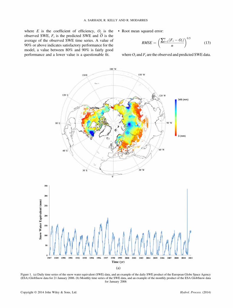
where E is the coefficient of efficiency, Oi is theobserved SWE, Fi is the predicted SWE and O is theaverage of the observed SWE time series. A value of90% or above indicates satisfactory performance for themodel, a value between 80% and 90% is fairly goodperformance and a lower value is a questionable fit.

(

Tim

Snow

Wat

er E

quiv

alen

t (m

m)

Figure 1. (a) Daily time series of the snow water equivalent (SWE) data, and a(ESA) GlobSnow data for 21 January 2006. (b) Monthly time series of the SW

for Januar


• Root mean squared error:

RMSE ¼ ∑ni¼1 Fi � Oið Þ

n

� �0:5

(13)

whereOi andFi are the observed and predicted SWEdata.

a)

e (yr)

n example of the daily SWE product of the European Globe Space AgencyE data, and an example of the monthly product of the ESA GlobSnow datay 2006


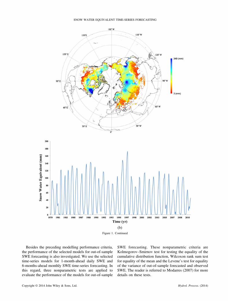
Figure 1. Continued


Besides the preceding modelling performance criteria,the performance of the selected models for out-of-sampleSWE forecasting is also investigated. We use the selectedtime-series models for 1-month-ahead daily SWE and6-months-ahead monthly SWE time-series forecasting. Inthis regard, three nonparametric tests are applied toevaluate the performance of the models for out-of-sample


SWE forecasting. These nonparametric criteria areKolmogorov–Smirnov test for testing the equality of thecumulative distribution function, Wilcoxon rank sum testfor equality of the mean and the Levene’s test for equalityof the variance of out-of-sample forecasted and observedSWE. The reader is referred to Modarres (2007) for moredetails on these tests.



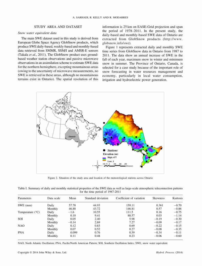
STUDY AREA AND DATASET

Snow water equivalent data

The main SWE dataset used in this study is derived fromEuropean Globe Space Agency GlobSnow products, whichproduce SWEdaily-based,weekly-based andmonthly-baseddata retrieved from SMMR, SSM/I and AMSR-E sensors(Takala et al., 2011). The GlobSnow product uses ground-based weather station observations and passive microwaveobservations in an assimilation scheme to estimate SWEdatafor the northern hemisphere, excepting mountainous areas(owing to the uncertainty of microwavemeasurements, noSWE is retrieved in these areas, although no mountainousterrains exist in Ontario). The spatial resolution of this

Figure 2. Situation of the study area and location

Table I. Summary of daily and monthly statistical properties of the Sfor the time perio

Parameters Data scale Mean Standard devi

SWE (mm) Daily 57.78 44.93Monthly 46.88 43.72

Temperature (°C) Daily �1.6 10.55Monthly 0.10 9.41

SOI Daily 0.05 2.40Monthly �0.14 2.69

NAO Daily 0.12 0.83Monthly 0.07 0.52

PNA Daily 0.099 0.76Monthly 0.11 0.48

NAO, North Atlantic Oscillation; PNA, Pacific/North American Pattern; SO


information is 25 km on EASE-Grid projection and spanthe period of 1978–2011. In the present study, thedaily-based and monthly-based SWE data of Ontario areextracted from GlobSnow products (http://www.globsnow.info/swe).Figure 1 represents extracted daily and monthly SWE

time series from GlobSnow data in Ontario from 1987 to2011. The data show an annual increase of SWE in thefall of each year, maximum snow in winter and minimumsnow in summer. The Province of Ontario, Canada, isselected for a case study because of the important role ofsnow forecasting in water resources management andeconomy, particularly in local water consumption,irrigation and hydroelectric power generation.

StationsElevation (m)

High: 677

Low: 1

of the meteorological stations across Ontario

WE data as well as large-scale atmospheric teleconnection patternsd of 1987-2011

ation Coefficient of variation Skewness Kurtosis

159.11 0.361 �0.70146.81 0.57 �0.86111.5 0.16 �0.7588.57 0.03 �1.145.98 �0.19 �0.307.27 �0.09 �0.170.69 �0.22 �0.150.27 �0.08 �0.350.59 �0.34 �0.110.23 �0.06 �0.60

I, Southern Oscillation Index; SWE, snow water equivalent.


http://www.globsnow.info/swe

http://www.globsnow.info/swe


Exogenous variables

Anumber of studies have demonstrated the linkage betweensnow features and variability of large-scale atmosphericcirculation patterns in different parts of Canada. Forexample, Zhao et al. (2013) studied the relationship of thePacific/North American Pattern (PNA) and North AtlanticOscillation (NAO) to the annual maximum SWE(SWEmax) anomalies over southern parts of Canada. Theyfound that SWEmax is significantly correlated with theNAO variations in eastern Canada, especially over centralOntario, while the correlation in western Canada is more

Table II. Pearson correlation coefficients between the daily andmonthly SWE data and climatic indices

SWE Temperature PNA NAO SOI

Daily based �0.334** 0.019 0.213** �0.070**Monthly based �0.832** 0.127* 0.268** �0.034

NAO, North Atlantic Oscillation; PNA, Pacific/North American Pattern;SOI, Southern Oscillation Index; SWE, snow water equivalent.**p< 0.01;*p< 0.05.

Figure 3. Autocorrelation function of the nonseasonal daily time serie

Table III. Multicriteria comparison of the best selected m

Group Models Exogenous variables

1 ARMA(1, 1) —2 TT-ARMA(1, 1) —3 ARMAX(1, 1) Temperature

NAOSOIPNANAO, SOI, PNA, temperatur

4 TT-ARMAX(1, 1) NAO, SOI, PNA, temperatur

ARMA, autoregressive moving-average model; ARMAX, autoregressive movIoAd, index of agreement; MAE, mean absolute error; NAO, North Atlantic Oerror; SOI, Southern Oscillation Index; SWE, snow water equivalent; TT, ti


closely associated with PNA variations. Similar resultshave also been reported in other studies of snow cover(Gutzler and Rosen, 1992; Karl et al., 1993; Saito et al.,2004; Brown, 2010).Therefore, in this study, we apply three main large-

scale atmospheric indices, PNA, NAO and SouthernOscillation Index (SOI), together with temperature as theexogenous variable for SWE time-series modelling andforecasting.Daily indices of the NAO and PNA are obtained from

the Climate Prediction Center, NOAA/National WeatherService (ftp://ftp.cpc.ncep.noaa.gov/cwlinks/), and valuesof the SOI (obtained from http://www.cpc.ncep.noaa.gov/data/indices/soi) are converted into a daily scale by usinga linear interpolation approach to produce daily SOIvalues for comparing the indices in the same scale(Rasouli et al., 2012). To evaluate the monthly variationsof the NAO and PNA indices, a monthly time series isformed using an average function, which measures thecentral tendency of the daily indices. In addition, in orderto evaluate the effect of local recorded meteorologicalfactors on the SWE data, mean temperatures from 24meteorological stations distributed across Ontario

s of the snow water equivalent (solid lines show confidence levels)

odels for the daily snow water equivalent time series

R2 RMSE MAE IoAd CE

0.956 8.53 7.80 0.71 0.9680.968 8.02 3.90 0.89 0.9670.968 8.02 3.90 0.85 0.9680.983 5.93 3.62 0.97 0.9830.983 5.94 3.69 0.96 0.9810.968 8.02 3.90 0.87 0.968

e 0.983 5.91 3.61 0.98 0.983e 0.984 5.92 3.61 0.99 0.985

ing-average model with exogenous variables; CE, coefficient of efficiency;scillation; PNA, Pacific/North American Pattern; RMSE, root mean squareme trend.


http://www.cpc.ncep.noaa.gov/data/indices/soi

http://www.cpc.ncep.noaa.gov/data/indices/soi


(Figure 2) are applied at two timescales: daily andmonthly. The variables are assembled for the 1987–2011period.After extraction of the daily time series from GlobSnow

data, SWE data are converted into monthly-based data byusing the average of the daily data for each month. Thestatistical characteristics of the two SWE time series (dailyand monthly), the atmospheric teleconnection patterns

Table IV. Estimated parameters for the TT-ARMAX(1, 1) fordaily time series

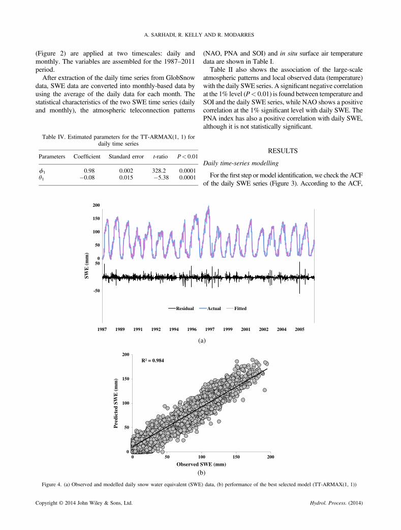
arameters Coefficient Standard error t-ratio P< 0.01

1 0.98 0.002 328.2 0.00011 �0.08 0.015 �5.38 0.0001

P

ϕθ

(a

1987 1989 1991 1992 1994 1996

Residual

200

150

100

50

0

SWE

(m

m)

50

-50

(b

R² = 0.984

0

50

100

150

200

0 50 10

Pre

dict

ed S

WE

(m

m)

Observed S

Figure 4. (a) Observed and modelled daily snow water equivalent (SWE)


(NAO, PNA and SOI) and in situ surface air temperaturedata are shown in Table I.Table II also shows the association of the large-scale

atmospheric patterns and local observed data (temperature)with the daily SWE series. A significant negative correlationat the 1% level (P< 0.01) is found between temperature andSOI and the daily SWE series, while NAO shows a positivecorrelation at the 1% significant level with daily SWE. ThePNA index has also a positive correlation with daily SWE,although it is not statistically significant.

RESULTS

Daily time-series modelling

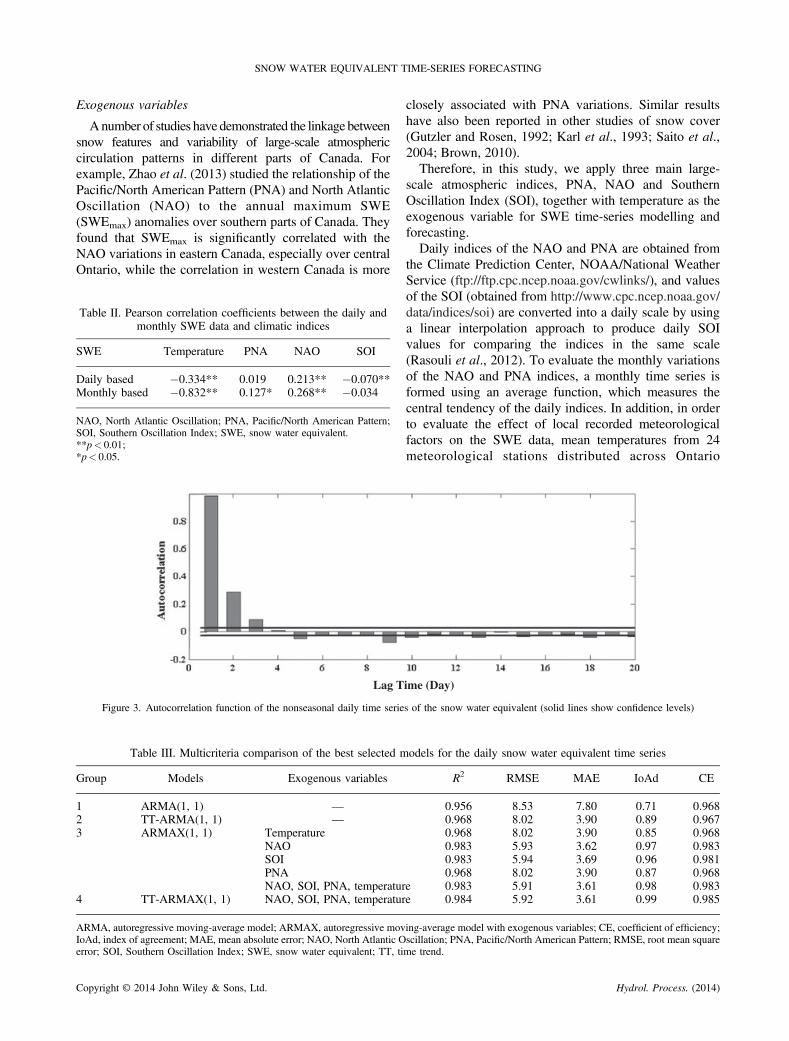
For the first step or model identification, we check the ACFof the daily SWE series (Figure 3). According to the ACF,

)

1997 1999 2001 2002 2004 2005

Actual Fitted

)

0 150 200

WE (mm)

data, (b) performance of the best selected model (TT-ARMAX(1, 1))



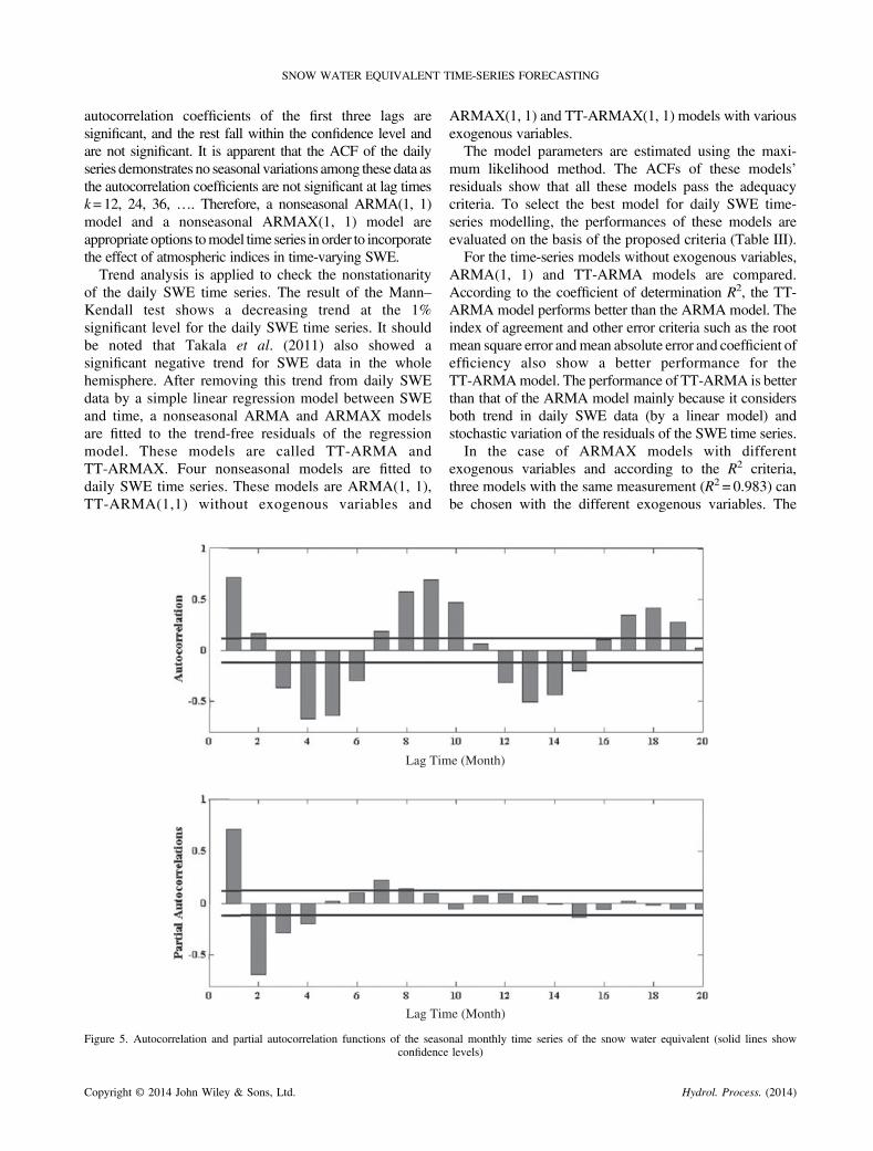
autocorrelation coefficients of the first three lags aresignificant, and the rest fall within the confidence level andare not significant. It is apparent that the ACF of the dailyseries demonstrates no seasonal variations among these data asthe autocorrelation coefficients are not significant at lag timesk=12, 24, 36, …. Therefore, a nonseasonal ARMA(1, 1)model and a nonseasonal ARMAX(1, 1) model areappropriate options tomodel time series in order to incorporatethe effect of atmospheric indices in time-varying SWE.Trend analysis is applied to check the nonstationarity

of the daily SWE time series. The result of the Mann–Kendall test shows a decreasing trend at the 1%significant level for the daily SWE time series. It shouldbe noted that Takala et al. (2011) also showed asignificant negative trend for SWE data in the wholehemisphere. After removing this trend from daily SWEdata by a simple linear regression model between SWEand time, a nonseasonal ARMA and ARMAX modelsare fitted to the trend-free residuals of the regressionmodel. These models are called TT-ARMA andTT-ARMAX. Four nonseasonal models are fitted todaily SWE time series. These models are ARMA(1, 1),TT-ARMA(1,1) without exogenous variables and

Lag Tim

Lag Tim

Figure 5. Autocorrelation and partial autocorrelation functions of the seasoconfidence


ARMAX(1, 1) and TT-ARMAX(1, 1) models with variousexogenous variables.The model parameters are estimated using the maxi-

mum likelihood method. The ACFs of these models’residuals show that all these models pass the adequacycriteria. To select the best model for daily SWE time-series modelling, the performances of these models areevaluated on the basis of the proposed criteria (Table III).For the time-series models without exogenous variables,

ARMA(1, 1) and TT-ARMA models are compared.According to the coefficient of determination R2, the TT-ARMA model performs better than the ARMA model. Theindex of agreement and other error criteria such as the rootmean square error andmean absolute error and coefficient ofefficiency also show a better performance for theTT-ARMAmodel. The performance of TT-ARMA is betterthan that of the ARMA model mainly because it considersboth trend in daily SWE data (by a linear model) andstochastic variation of the residuals of the SWE time series.In the case of ARMAX models with different

exogenous variables and according to the R2 criteria,three models with the same measurement (R2 = 0.983) canbe chosen with the different exogenous variables. The

e (Month)

e (Month)

nal monthly time series of the snow water equivalent (solid lines showlevels)



index of agreement measure and error criteria demon-strate that the ARMAX model with a combination of allthe independent variables has a slightly betterperformance than the alternative models. Typically, inthe case of having similar models and similar perfor-mances, the model with the least parameters is selected asthe best model (Haltiner and Salas, 1988). The ARMAX(1, 1) model with only one exogenous variable (NAO) isselected as the best model.Comparing the ARMAX model with the trend-free

model of TT-ARMAX indicates that the approach formodelling daily SWE time series in the presence of asignificant trend, TT-ARMAX (1, 1), performs better thanthe ARMAX(1, 1) model. Table IV presents parametersfor the selected model. The observed and estimated dailySWE time series (Figure 4a) and the scatter plot between

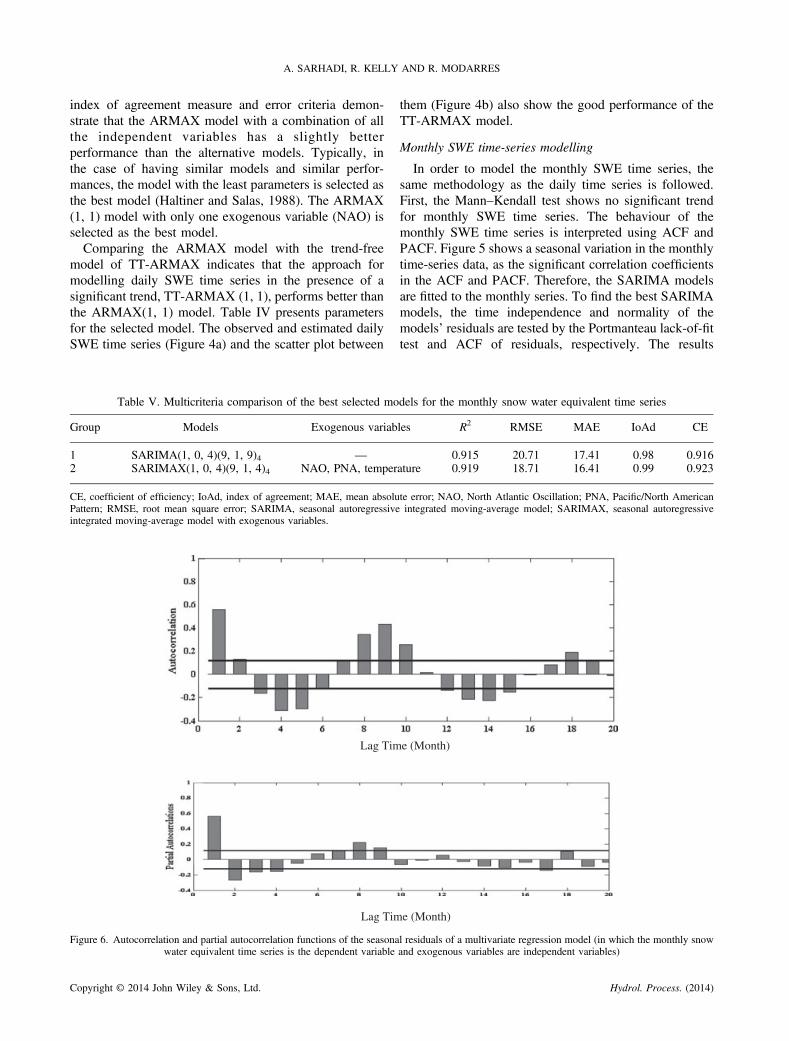
Table V. Multicriteria comparison of the best selected mo

Group Models Exogenous variab

1 SARIMA(1, 0, 4)(9, 1, 9)4 —2 SARIMAX(1, 0, 4)(9, 1, 4)4 NAO, PNA, temper

CE, coefficient of efficiency; IoAd, index of agreement; MAE, mean absoluPattern; RMSE, root mean square error; SARIMA, seasonal autoregressiveintegrated moving-average model with exogenous variables.

Lag Tim

Lag Tim

Figure 6. Autocorrelation and partial autocorrelation functions of the seasonawater equivalent time series is the dependent variable


them (Figure 4b) also show the good performance of theTT-ARMAX model.

Monthly SWE time-series modelling

In order to model the monthly SWE time series, thesame methodology as the daily time series is followed.First, the Mann–Kendall test shows no significant trendfor monthly SWE time series. The behaviour of themonthly SWE time series is interpreted using ACF andPACF. Figure 5 shows a seasonal variation in the monthlytime-series data, as the significant correlation coefficientsin the ACF and PACF. Therefore, the SARIMA modelsare fitted to the monthly series. To find the best SARIMAmodels, the time independence and normality of themodels’ residuals are tested by the Portmanteau lack-of-fittest and ACF of residuals, respectively. The results

dels for the monthly snow water equivalent time series

les R2 RMSE MAE IoAd CE

0.915 20.71 17.41 0.98 0.916ature 0.919 18.71 16.41 0.99 0.923

te error; NAO, North Atlantic Oscillation; PNA, Pacific/North Americanintegrated moving-average model; SARIMAX, seasonal autoregressive

e (Month)

e (Month)

l residuals of a multivariate regression model (in which the monthly snowand exogenous variables are independent variables)


(a)

1987 1990 1993 1997 2000 2003 2007 2010

Residual Actual

Fitted

Time

SWE

(m

m)

-40

(b)

R² = 0.919

Pre

dict

ed S

WE

(m

m)

Observed SWE (mm)

00 50 100 150 200

50

100

150

200

40

0

50

100

150

200

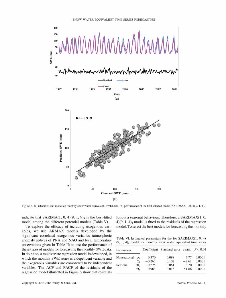
Figure 7. (a) Observed and modelled monthly snow water equivalent (SWE) data, (b) performance of the best selected model (SARIMAX(1, 0, 4)(9, 1, 4)4)

Table VI. Estimated parameters for the for SARIMAX(1, 0, 4)(9, 1, 4)4 model for monthly snow water equivalent time series

Parameters Coefficient Standard error t-ratio P< 0.01

Nonseasonal ϕ1 0.370 0.098 3.77 0.0001θ4 �0.267 0.102 �2.61 0.0001

Seasonal Φ9 �0.225 0.061 �3.70 0.0001Θ4 0.963 0.018 51.86 0.0001


indicate that SARIMA(1, 0, 4)(9, 1, 9)4 is the best-fittedmodel among the different potential models (Table V).To explore the efficacy of including exogenous vari-

ables, we use ARMAX models developed by thesignificant correlated exogenous variables (atmosphericanomaly indices of PNA and NAO and local temperatureobservations given in Table II) to test the performance ofthese types of models for forecasting themonthly SWEdata.In doing so, a multivariate regressionmodel is developed, inwhich the monthly SWE series is a dependent variable andthe exogenous variables are considered to be independentvariables. The ACF and PACF of the residuals of theregression model illustrated in Figure 6 show that residuals


follow a seasonal behaviour. Therefore, a SARIMAX(1, 0,4)(9, 1, 4)4 model is fitted to the residuals of the regressionmodel. To select the best models for forecasting the monthly



SWE time series, performance criteria are assessed. Resultsof the performance analysis (given in Table V) reveal thatSARIMAX(1, 0, 4)(9, 1, 4)4 represents a better performancethan the SARIMA(1, 0, 4)(9, 1, 9)4model. The time series ofthe observed and predicted values of the monthly SWE timeseries for the best model, as well as their scatter plot, aregiven in Figure 7. The parameters of the selected model are

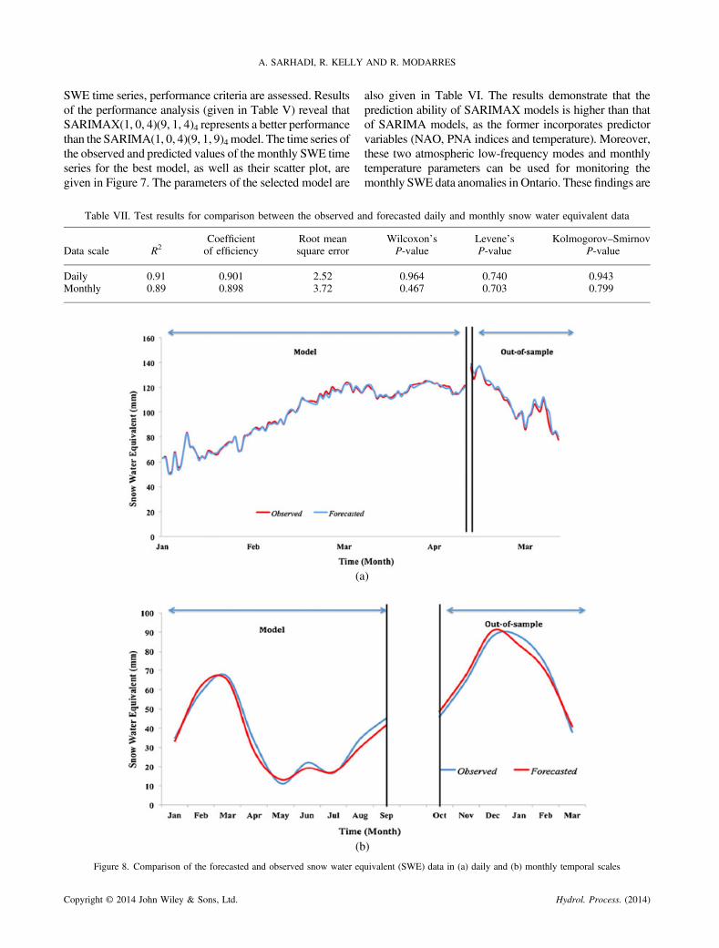
Table VII. Test results for comparison between the observed a

Data scale R2Coefficientof efficiency

Root meansquare error

Daily 0.91 0.901 2.52Monthly 0.89 0.898 3.72

(a

(b

Figure 8. Comparison of the forecasted and observed snow water eq


also given in Table VI. The results demonstrate that theprediction ability of SARIMAX models is higher than thatof SARIMA models, as the former incorporates predictorvariables (NAO, PNA indices and temperature). Moreover,these two atmospheric low-frequency modes and monthlytemperature parameters can be used for monitoring themonthly SWE data anomalies in Ontario. These findings are

nd forecasted daily and monthly snow water equivalent data

Wilcoxon’sP-value

Levene’sP-value

Kolmogorov–SmirnovP-value

0.964 0.740 0.9430.467 0.703 0.799

)

)

uivalent (SWE) data in (a) daily and (b) monthly temporal scales



consistent with the findings of Zhao et al. (2013) andNotaro et al. (2006) who showed how the combination ofthe NAO and PNA anomalies affect SWE anomalies andcan explain more variance of SWE time-series variation ineastern Canada.

Out-of-sample forecasting

To assess the validity of the best selected models in theprevious sections for the two temporal scales, thesemodels are used for out-of-sample daily and monthlySWE forecasting. As time-series modelling is used forforecasting hydroclimatic variables in short-term periods(Haltiner and Salas, 1988), we select a period of 1month(from 21 April 2011 to 21 May 2011) and a period of6months (from December 2010 until May 2011) forforecasting the daily and monthly SWE time series,respectively. The results of the criteria, which aredescribed in the Section on Model Performance and usedto compare observed and out-of-sample forecasted SWEtime series, are given in Table VII. The results show nosignificant difference between observed and forecastedSWE time series for both timescales. The correlationcoefficient indicates a highly satisfactory forecasting, andthe root mean square errors as well as the coefficient ofefficiency measurements show a good performance forboth temporal scales. The P-values of Wilcoxon andLevene, which are larger than 0.05, indicate that there isno difference between the mean and variance of theforecasted and observed SWE time series. In addition, theKolmogorov–Smirnov criterion demonstrates that there isno difference between distribution functions of theforecasted and observed SWE time series. The resultsalso reveal a slightly better performance of the selectedmodel for SWE daily time series than that for the monthlySWE time series.The forecasted daily and monthly SWE data and

corresponding observed data are illustrated in Figure 8.This figure indicates a good agreement between observedand modelled SWE time series for both time series. Themodelled SWE daily time series follows the increasingvariation of the observed SWE from January to April inexcellent agreement (Figure 8a). In addition, the out-of-sample forecasted SWE time series is well fitted to theobserved time series, indicating that the TT-ARMAXperforms best for forecasting daily SWE time series. Thisis mainly due to adding the time trend of SWE and theeffect of exogenous variables into the stochastic model.These conditions are also observed for monthly SWE

time-series models (Figure 8b). The estimated SWE timeseries follows the observed seasonal SWE time seriesvery well from January to September. This very goodagreement is also observed between observed andforecasted monthly SWE time series. These results also


show the importance of incorporating appropriate exog-enous variables for SWE time-series forecasting.

SUMMARY AND CONCLUSION

In the present study, an SWE time series extracted fromremotely sensed GlobSnow data is modelled by differenttime-series approaches in two, daily and monthly,timescales for Ontario, Canada. The most importantcontribution of this study is the time-series modelling of adaily SWE series in the presence of a trend and theSARIMA modelling of a monthly SWE series. For thedaily SWE series, which shows a significant negativetrend, four different types of nonseasonal time-seriesmodels, namely ARMA, TT-ARMA, ARMAX andTT-ARMAX, are applied to select the best model forpredicting the daily SWE data. The results reveal that anARMA model incorporating both time trend andexogenous variables (i.e. the TT-ARMAX model) fordaily SWE time series outperforms the models withouttrend parameters and atmospheric anomaly variables.Therefore, this type of ARMAX model is strongly

suggested for time-series modelling of the daily andmonthly SWE time series and other hydroclimaticvariables that have a significant trend. For the seasonalmonthly SWE time series, which shows no significanttrend, two SARIMA and SARIMAX models are fitted.The multicriteria performance evaluation indicates thatincorporating exogenous variables into a SARIMA willimprove the performance of the SARIMA model. Theresults indicate that SWE is more dependent on NAO thanon other teleconnection indices (PNA and SOI) and itsvariation could be used for predicting SWE variations ofOntario. These results are consistent with the study of Zhaoet al. (2013), which indicates that SWEdata are significantlycorrelated with the NAO index over central Ontario.The use of the selected model for out-of-sample short-

term forecasting suggests that the selected models have asatisfactory validity and are reliable for short-termforecasting the daily and monthly SWE data for Ontario.It is suggested that the selected models for daily and

monthly scales (TT-ARMAX and SARIMAX models) betested in different regions and, perhaps, for other snowcharacteristics such as snow cover extent. Taking intoaccount other atmospheric anomaly variables and othertemperature parameters such as daily and monthlyabsolute minimum and maximum temperatures andprecipitation for SWE time-series modelling and fore-casting is also suggested for future studies. As theselected models are linear and might encompass someinadequacies in performances, application of nonlinearand multivariate time-series models coupled with theexogenous variables applied in this study and other



variables is highly recommended for seasonal andnonseasonal modelling and forecasting of the SWE timeseries in further studies.

REFERENCES

Box GEP, Jenkins GM. 1976. Time Series Analysis: Forecasting andControl, revised edn. Holden Day: San Francisco.

Brown RD. 2010. Analysis of snow cover variability and change inQuébec 1948–2005. Hydrological Processes 24(14): 1929–1954.

Dery SJ, Sheffield J, Wood EF. 2005. Connectivity between Eurasiansnow cover extent and Canadian snow water equivalent and riverdischarge. Journal of Geophysical Resources 110: D23106.

Gutzler D, Rosen RD. 1992. Interannual variability of wintertime snow coveracross the Northern Hemisphere. Journal of Climate 5: 1441–1447.

Haltiner JP, Salas JD. 1988. Short-term forecasting of snowmelt runoffusing ARMAX models. Journal of the American Water ResourcesAssociation 24(5): 1083–1089.

Hipel KW, McLeod AE. 1994. Time Series Modeling of Water Resourcesand Environmental Systems. Elsevier: Amsterdam, The Netherlands.

Karamouz M, Zahraie B. 2004. Seasonal streamflow forecasting using snowbudgetandElNiño-SouthernOscillationclimatesignals:applicationtotheSaltRiver Basin in Arizona. Journal of Hydrologic Engineering 9(6): 523–533.

Karl TR, Groisman PY, Knight RW, Heim RRJ. 1993. Recent variations ofsnow cover and snowfall in North America and their relation toprecipitation and temperature variations. Journal of Climate 6: 1327–1344.

KendallMG. 1975.RankCorrelationMeasures. Charle Griffin: London,UK.Mann HB. 1945. Nonparametric tests against trend. Econometrica 13(3):245–259.

McNamara JP, Kane DL, Hinzman LD. 1998. An analysis of streamflowhydrology in the Kuparuk River Basin, Alaska: a nested watershedapproach. Journal of Hydrology 206: 39–57.


Mishra AK, Desai VR. 2005. Drought forecasting using stochasticmodels. Stochastic Environmental Research and Risk Assessment 19(5):326–339.

Modarres R. 2007. Streamflow drought time series forecasting. StochasticEnvironmental Research and Risk Assessment 21: 223–233.

Modarres R, Ouarda TBMJ, Vanasse A, Orzanco MG, Gosselin P. 2012.Modeling seasonal variation of hip fracture in Montreal, Canada. Bone50: 909–916.

Nash JE, Sutcliffe JV. 1970. River flow forecasting through. Part I. Aconceptual models discussion of principles. Journal of Hydrology 10:282–290.

Notaro M, Wang WC, Gong W. 2006. Model and observational analysisof the northeast U.S. regional climate and its relationship to the PNAand NAO patterns during early winter. Monthly Weather Review 134:3479–3505.

Rasouli K, Hsieh WW, Cannon AJ. 2012. Daily streamflow forecasting bymachine learning methods with weather and climate inputs. Journal ofHydrology 414: 284–293.

Saito K, Yasunari T, Cohen J. 2004. Changes in the sub-decadalcovariability between northern hemisphere snow cover and the generalcirculation of the atmosphere. International Journal of Climatology 24:33–44.

Salas JD, Delleur JW, Yevjevich VM, Lane WL. 1980. Applied Modelingof Hydrologic Time Series. Water Resources Publications: Littleton.

Soltani S, Modarres R, Eslamian SS. 2007. The use of time seriesmodeling for the determination of rainfall climates of Iran. InternationalJournal of Climatology 27: 819–829.

Takala M, Luojus K, Pulliainen J, Derksen C, Lemmetyinen J, Kärnä J,Koskinen J, Bojkov B. 2011. Estimating northern hemisphere snowwater equivalent for climate research through assimilation of space-borne radiometer data and ground-based measurements. RemoteSensing of Environment 115(12): 3517–3529.

Zhao H, Higuchi K, Waller J, Auld H, Mote T. 2013. The impacts of thePNA and NAO on annual maximum snowpack over southern Canadaduring 1979–2009. International Journal of Climatology 33: 388–395.


Snow water equivalent time-series forecasting in Ontario, Canada, in link to large atmospheric circulations

Documents