Snow, ice and solar radiation Peter Kuipers Munneke

Welcome message from author
This document is posted to help you gain knowledge. Please leave a comment to let me know what you think about it! Share it to your friends and learn new things together.
Transcript
Snow, ice and solar radiation
Peter Kuipers Munneke

Snow, ice and solar radiationSneeuw, ijs en zonnestraling
(met een samenvatting in het Nederlands)
PROEFSCHRIFT
ter verkrijging van de graad van doctor aan deUniversiteit Utrecht op gezag van de rector magnificus,
prof. dr. J.C. Stoof, ingevolge het besluit van hetcollege voor promoties in het openbaar te verdedigen
op 14 oktober 2009 des middags te 4.15 uur
door
Peter Kuipers Munneke
geboren op 31 maart 1980 te Groningen

Promotor: Prof. dr. J. OerlemansCo-promotor: Dr. C. H. Tijm-Reijmer


ii Contents
4 Analysis of clear-sky Antarctic snow albedo 474.1 Introduction . . . . . . . . . . . . . . . . . . . . . . . . . . . . . . . . . . . 484.2 Data and methods . . . . . . . . . . . . . . . . . . . . . . . . . . . . . . . . 484.3 Results . . . . . . . . . . . . . . . . . . . . . . . . . . . . . . . . . . . . . . 534.4 Discussion . . . . . . . . . . . . . . . . . . . . . . . . . . . . . . . . . . . . 564.5 Summary and conclusions . . . . . . . . . . . . . . . . . . . . . . . . . . . 58
5 Cloud properties from radiation measurements over snow and ice 615.1 Introduction . . . . . . . . . . . . . . . . . . . . . . . . . . . . . . . . . . . 625.2 Data and methods . . . . . . . . . . . . . . . . . . . . . . . . . . . . . . . . 635.3 Results . . . . . . . . . . . . . . . . . . . . . . . . . . . . . . . . . . . . . . 705.4 Applications . . . . . . . . . . . . . . . . . . . . . . . . . . . . . . . . . . . 765.5 Conclusions . . . . . . . . . . . . . . . . . . . . . . . . . . . . . . . . . . . 81
6 The energy budget of the snowpack at Summit, Greenland 836.1 Introduction . . . . . . . . . . . . . . . . . . . . . . . . . . . . . . . . . . . 846.2 Data . . . . . . . . . . . . . . . . . . . . . . . . . . . . . . . . . . . . . . . 856.3 The energy balance model . . . . . . . . . . . . . . . . . . . . . . . . . . . 866.4 Results and comparison with measurement data . . . . . . . . . . . . . . . . 896.5 Discussion and conclusions . . . . . . . . . . . . . . . . . . . . . . . . . . . 98
7 Spectral snow albedo and snow grain size 1017.1 Introduction . . . . . . . . . . . . . . . . . . . . . . . . . . . . . . . . . . . 1027.2 Data and methods . . . . . . . . . . . . . . . . . . . . . . . . . . . . . . . . 1037.3 Results . . . . . . . . . . . . . . . . . . . . . . . . . . . . . . . . . . . . . . 1077.4 Discussion and conclusions . . . . . . . . . . . . . . . . . . . . . . . . . . . 113
Bibliography 115
Dankwoord 123
Curriculum vitae 125
Publications 127
iv Samenvatting
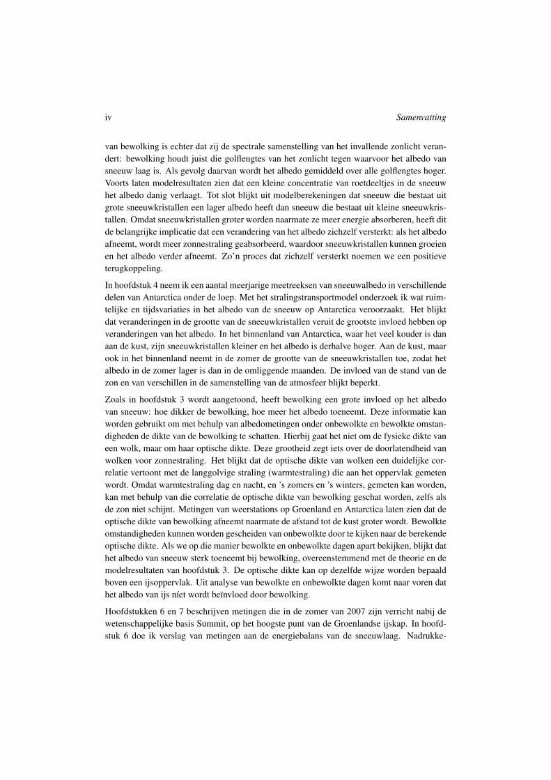
van bewolking is echter dat zij de spectrale samenstelling van het invallende zonlicht veran-dert: bewolking houdt juist die golflengtes van het zonlicht tegen waarvoor het albedo vansneeuw laag is. Als gevolg daarvan wordt het albedo gemiddeld over alle golflengtes hoger.Voorts laten modelresultaten zien dat een kleine concentratie van roetdeeltjes in de sneeuwhet albedo danig verlaagt. Tot slot blijkt uit modelberekeningen dat sneeuw die bestaat uitgrote sneeuwkristallen een lager albedo heeft dan sneeuw die bestaat uit kleine sneeuwkris-tallen. Omdat sneeuwkristallen groter worden naarmate ze meer energie absorberen, heeft ditde belangrijke implicatie dat een verandering van het albedo zichzelf versterkt: als het albedoafneemt, wordt meer zonnestraling geabsorbeerd, waardoor sneeuwkristallen kunnen groeienen het albedo verder afneemt. Zo’n proces dat zichzelf versterkt noemen we een positieveterugkoppeling.
In hoofdstuk 4 neem ik een aantal meerjarige meetreeksen van sneeuwalbedo in verschillendedelen van Antarctica onder de loep. Met het stralingstransportmodel onderzoek ik wat ruim-telijke en tijdsvariaties in het albedo van de sneeuw op Antarctica veroorzaakt. Het blijktdat veranderingen in de grootte van de sneeuwkristallen veruit de grootste invloed hebben opveranderingen van het albedo. In het binnenland van Antarctica, waar het veel kouder is danaan de kust, zijn sneeuwkristallen kleiner en het albedo is derhalve hoger. Aan de kust, maarook in het binnenland neemt in de zomer de grootte van de sneeuwkristallen toe, zodat hetalbedo in de zomer lager is dan in de omliggende maanden. De invloed van de stand van dezon en van verschillen in de samenstelling van de atmosfeer blijkt beperkt.
Zoals in hoofdstuk 3 wordt aangetoond, heeft bewolking een grote invloed op het albedovan sneeuw: hoe dikker de bewolking, hoe meer het albedo toeneemt. Deze informatie kanworden gebruikt om met behulp van albedometingen onder onbewolkte en bewolkte omstan-digheden de dikte van de bewolking te schatten. Hierbij gaat het niet om de fysieke dikte vaneen wolk, maar om haar optische dikte. Deze grootheid zegt iets over de doorlatendheid vanwolken voor zonnestraling. Het blijkt dat de optische dikte van wolken een duidelijke cor-relatie vertoont met de langgolvige straling (warmtestraling) die aan het oppervlak gemetenwordt. Omdat warmtestraling dag en nacht, en ’s zomers en ’s winters, gemeten kan worden,kan met behulp van die correlatie de optische dikte van bewolking geschat worden, zelfs alsde zon niet schijnt. Metingen van weerstations op Groenland en Antarctica laten zien dat deoptische dikte van bewolking afneemt naarmate de afstand tot de kust groter wordt. Bewolkteomstandigheden kunnen worden gescheiden van onbewolkte door te kijken naar de berekendeoptische dikte. Als we op die manier bewolkte en onbewolkte dagen apart bekijken, blijkt dathet albedo van sneeuw sterk toeneemt bij bewolking, overeenstemmend met de theorie en demodelresultaten van hoofdstuk 3. De optische dikte kan op dezelfde wijze worden bepaaldboven een ijsoppervlak. Uit analyse van bewolkte en onbewolkte dagen komt naar voren dathet albedo van ijs nıet wordt beınvloed door bewolking.
Hoofdstukken 6 en 7 beschrijven metingen die in de zomer van 2007 zijn verricht nabij dewetenschappelijke basis Summit, op het hoogste punt van de Groenlandse ijskap. In hoofd-stuk 6 doe ik verslag van metingen aan de energiebalans van de sneeuwlaag. Nadrukke-
Samenvatting v
lijk kijk ik naar de rol van zonnestraling in deze energiebalans. Hoogwaardige metingenvan zonnestraling, warmtestraling en meteorologische grootheden worden gebruikt als in-voer voor een model dat niet alleen de energiebalans van het sneeuwoppervlak berekent maarook de temperatuurverdeling in de sneeuw. Een vergelijking van gemodelleerde met geme-ten sneeuwtemperaturen leidt tot de hypothese dat zonnestraling die dieper in de sneeuwdoordringt wezenlijk bijdraagt aan de opwarming van de sneeuw en de temperatuurverdelingin de sneeuwlaag: zonder deze stralingspenetratie op te nemen in het energiebalansmodel,kunnen gemeten sneeuwtemperaturen niet gereconstrueerd worden. Metingen aan de groottevan de sneeuwkristallen worden gebruikt om ook door het stralingstransportmodel het effectvan stralingspenetratie te laten berekenen. De resultaten van deze berekeningen komen vrijgoed overeen met de resultaten van het energiebalansmodel. Ten slotte wordt aangetoond datzonnestraling veruit de belangrijkste bron van energie is voor de opwarming van het sneeuw-pakket. Deze toevoer van energie wordt voornamelijk gecompenseerd door netto uitstralingvan warmte, door opwarming van de sneeuw, door koeling van het sneeuwoppervlak doorwind, en door sublimatie van sneeuw.
In hoofdstuk 7 worden tot slot metingen van het albedo van sneeuw voor verschillende golf-lengtes geanalyseerd en vergeleken met modelberekeningen. In eerdere literatuur kondenmodelberekeningen alleen in overeenstemming worden gebracht met waarnemingen door teveronderstellen dat zich een zeer dun laagje van kleine sneeuwkristallen in de bovenste milli-meter van de sneeuwlaag bevond. In dit hoofdstuk laat ik met behulp van een stereografischeanalyse van digitale foto’s van sneeuwmonsters voor het eerst zien dat deze dunne laag ookinderdaad aanwezig is. De theorie van stralingstransport boven en in een sneeuwlaag wordthierdoor versterkt.

viii Summary
soot particles significantly lowers the albedo of the snowpack. Lastly, model calculationsshow that snow consisting of large snow grains has a lower albedo that snow consisting ofsmall snow grains. At the same time, snow grains are known to grow as they absorb moreenergy. This has the important implication that a change in albedo amplifies itself: whenthe albedo decreases, more solar radiation is absorbed, causing snow grains to grow and thealbedo to decrease further. Such a self-amplifying process is called a positive feedback.
In chapter 4, I study several multi-year series of snow albedo observations from various partsof Antarctica. Using the radiative transfer model, it is assessed which processes drive thespatial and temporal variability in snow albedo in Antarctica. It turns out that changes insnow grain size have by far the largest impact on variations of snow albedo. On the AntarcticPlateau, where temperatures are much lower than in the coastal regions, snow grains aresmaller and albedos higher. In coastal as well as inland regions, snow grain size is larger inthe summer months, resulting in reduced snow albedos compared to the spring and autumnmonths. The impact of variations of solar zenith angle and atmospheric composition are oflimited importance.
As demonstrated in chapter 3, cloud cover has a prominent influence on the albedo of snow.The increase of snow albedo with respect to clear-sky conditions is proportional to the opticalthickness of the cloud cover. This observation can be used to infer cloud optical thicknessfrom measurements of albedo under clear and cloudy conditions. It turns out that cloud op-tical thickness and the amount of longwave (thermal) radiation arriving at the surface areclearly correlated. Longwave radiation is recorded both day and night, and both in summerand winter, so the cloud optical thickness can be determined using this correlation, even in theabsence of solar radiation itself. Data from weather stations on the Greenland and Antarcticice sheets reveal that cloud optical thickness decreases away from the coast. Cloudy condi-tions can be separated from clear-sky conditions using computed cloud optical thickness. Byseparately studying clear and cloudy periods, snow albedo turns out to increase strongly inthe presence of clouds, conforming with theory and with the model results from chapter 3. Inthe same way, optical thickness can be determined above ice surfaces. Analysis of clear andcloudy days reveals that ice albedo is not influenced by the presence of clouds.
Chapters 6 and 7 deal with a measurement campaign carried out at the scientific base at Sum-mit, Greenland, in the summer of 2007. The Greenland Environmental Observatory at Sum-mit is located near the highest point of the Greenland ice sheet. In chapter 6, measurementsof the energy budget of the snowpack are presented, focussing on the role of solar radia-tion. State-of-the-art measurements of solar and thermal radiation, as well as meteorologicalvariables, are used as input for an energy balance model that also computes the tempera-ture distribution within the snowpack. A comparison between modelled and observed snowtemperatures suggests that subsurface absorption of penetrated solar radiation contributes sig-nificantly to the warming of the snowpack and to its temperature distribution: observed snowtemperatures cannot be simulated when the radiation penetration term is omitted from the en-ergy balance. Observations of snow grain size profiles are prescribed in the radiative transfer

Summary ix
model to compute the effect of radiation penetration. The results of these calculations agreereasonably well with the results from the energy balance model. Furthermore, we show thatshortwave radiation is by far the most important source of energy for heating of the snow-pack. The energy budget is closed by net emission of longwave radiation, by heating of thesnowpack, and by net negative sensible and latent heat fluxes.
In the final chapter, observations of spectral snow albedo are analysed and compared withspectral radiative transfer calculations. In previous literature, the presence of a submillimeterlayer of small snow grains had to be assumed to achieve agreement between model calcula-tions and field observations of spectral snow albedo. In this chapter, stereographic analysisof snow grain images shows, for the first time, the this submillimeter layer is actually presentin natural snow, reinforcing the theory of radiative transfer in and over a snow layer.

1Snow, ice and climate
1.1 The role of solar radiation in the climate system
Climate on Earth is, to a large extent, driven by the radiation it receives from the Sun. Theenergy required for many climatic processes on Earth is ultimately provided by solar radia-tion.
Solar radiation heats the atmosphere, the land and the oceans. However, the amount of solarradiation is not distributed evenly over the globe. Due to the spherical geometry of the Earth,the radiative energy of a beam of solar radiation is spread over a larger surface area in the polarregions than around the equator. As a consequence, there is more solar radiation availableat the equator than at the poles, and thus, the equatorial region is heated more than the polarregions. With respect to the global average, there is an excess of heat at the equator, anda deficit near the poles. A continuous poleward transport, both by the oceans and by theatmosphere, attempts to cancel this imbalance. The exact relative contribution of oceanicand atmospheric transport has been debated for decades, but they are of the same order ofmagnitude.
The atmospheric poleward transport of air and heat is affected by the rotation of the Earth,leading to some characteristic climatic phenomena. At tropical and subtropical latitudes(roughly between 30#N and 30#S), it gives rise to the Hadley circulation. In this circula-tion, air ascends in a band region known as the intertropical convergence zone, characterizedby the formation of large convective clouds and vigorous vertical mixing of the atmosphere.The migration of the intertropical convergence zone is dictated by the seasonal oscillationof the solar zenith point around the equator, and causes distinctive dry and wet seasons inthe tropics. The air aloft is transported poleward, before descending over the subtropics. Asthe air moves downward, the air is heated adiabatically, which suppresses the formation ofclouds and precipitation. Arid regions are therefore found around 30#N and 30#S. To closethe circulation in the Hadley cell, air is transported back to the tropics at the surface by thetrade winds. At middle latitudes, the interplay between atmospheric poleward transport andthe Earth’s rotation leads to the formation of large low- and high-pressure systems that governweather and climate in temperate regions.
1
2 1.2. The albedo of snow and ice
The relative energy deficit at the poles due to the Earth’s geometry is amplified by the pres-ence of snow and ice, that cover large parts of the Earth’s polar regions. Snow and ice surfacesin polar regions act as large ‘mirrors’ for solar radiation, and reflect most of it back to space.As a consequence, the amount of energy absorbed by the climate system is reduced evenmore than from geometric considerations only.
The extent of snow and ice cover on Earth is considerable, and consists of large continentalice masses (ice sheets) as well as vast expanses of frozen ocean (sea ice). On the NorthernHemisphere, the Arctic Ocean occupies most of the area north of the Polar Circle. About 5 to7 million km2 of the Arctic Ocean is covered with multi-year sea ice that survives through-out the year. In winter, sea-ice cover increases to 15 to 17 million km2 (for reference, theland surface area of Europe is approximately 10 million km2). Furthermore, the Northernhemisphere features the Greenland ice sheet, which has an area of 1,700,000 km2 and a vol-ume of 2,900,000 km3 (a potential sea-level rise of 7.3 m). On the Southern Hemisphere, theAntarctic Ice Sheet occupies an area of 12,300,000 km2 and has a volume of 24,700,000 km3
(potential sea-level rise of 56.6 m). At approximately 3 million km2, the area of multi-yearsea ice around Antarctica is much smaller than its Northern Hemisphere counterpart. In win-ter, sea-ice cover at the Southern Hemisphere increases to $19 million km2.
As discussed above, these vast areas of snow and ice reduce the amount of energy that entersthe climate system in the polar regions, leading to a lower surface temperature. Thanks tothese low temperatures, snow and ice can continue to exist. In other words, ice sheets andsea ice partly sustain their own presence. There is thus a very tight connection between solarradiation and climate in polar regions, owing to the presence of snow and ice. It will notcome as a surprise that snow and ice have been playing a crucial role in the history of Earth’sclimate. Before we can discuss the role of snow and ice in past and present climate however,we will need to better understand their optical properties.
1.2 The albedo of snow and ice
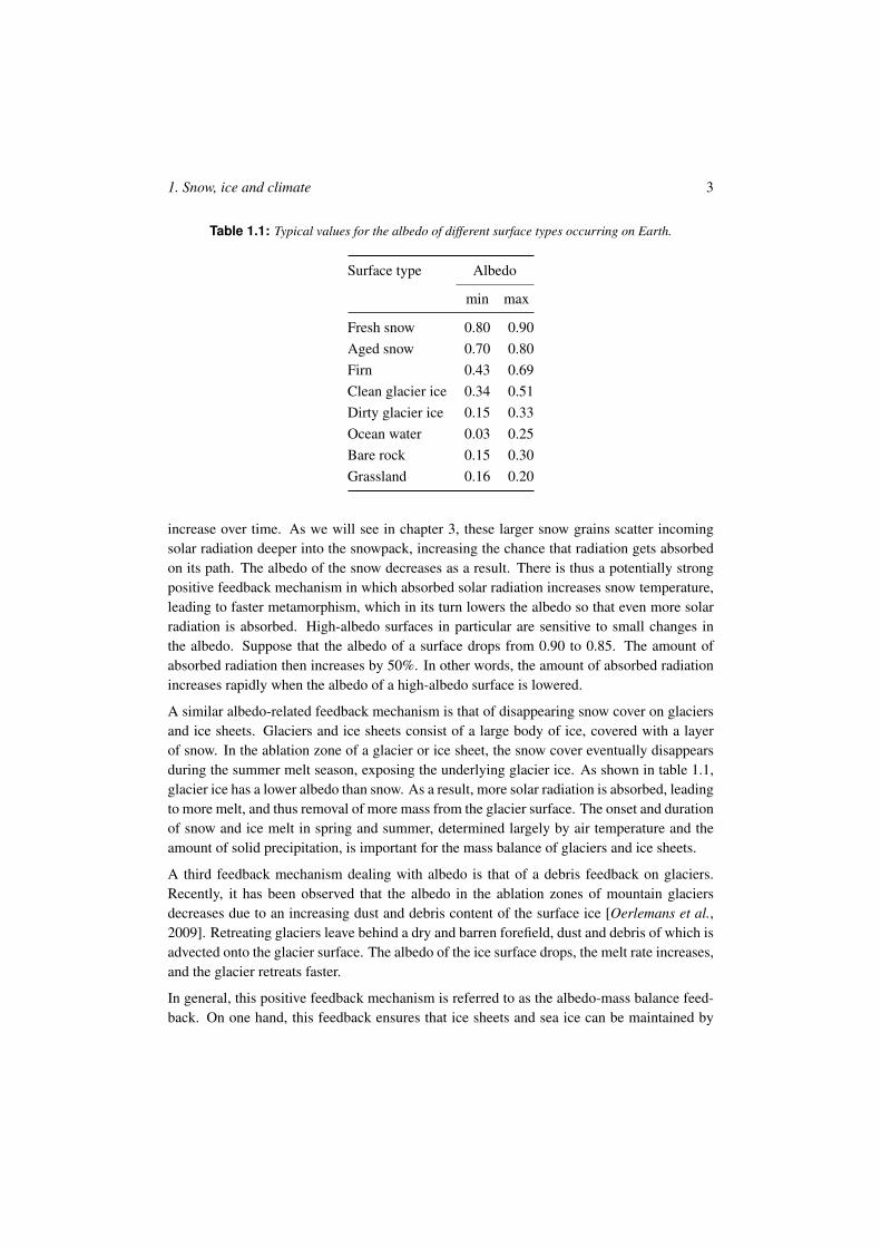
The fraction of solar radiation that is reflected by a surface is referred to as albedo, denoted by! . An albedo of 0.4 means that 40% of the incident solar radiation is reflected. The remaining60% is absorbed by the surface. Snow and ice surfaces generally have a high albedo, rangingfrom 0.4 for ice to 0.9 for clean and fresh dry snow. A list of the typical albedo for differentsurfaces is shown in table 1.1. It is apparent that most snow and ice surfaces have a muchhigher albedo than other surface types.
Snow and ice albedo depend on many factors, which will be discussed extensively in chap-ters 3 and 4. One of the most important factors for snow albedo is the size of the snowgrains that constitute the snowpack. Snow grains constantly evolve under the influence oftemperature and temperature gradients in the snow [Flanner and Zender, 2006], a processwhich is referred to as snow metamorphism. The effective size of the snow grains tends to
1. Snow, ice and climate 3
Table 1.1: Typical values for the albedo of different surface types occurring on Earth.
Surface type Albedo
min max
Fresh snow 0.80 0.90Aged snow 0.70 0.80Firn 0.43 0.69Clean glacier ice 0.34 0.51Dirty glacier ice 0.15 0.33Ocean water 0.03 0.25Bare rock 0.15 0.30Grassland 0.16 0.20
increase over time. As we will see in chapter 3, these larger snow grains scatter incomingsolar radiation deeper into the snowpack, increasing the chance that radiation gets absorbedon its path. The albedo of the snow decreases as a result. There is thus a potentially strongpositive feedback mechanism in which absorbed solar radiation increases snow temperature,leading to faster metamorphism, which in its turn lowers the albedo so that even more solarradiation is absorbed. High-albedo surfaces in particular are sensitive to small changes inthe albedo. Suppose that the albedo of a surface drops from 0.90 to 0.85. The amount ofabsorbed radiation then increases by 50%. In other words, the amount of absorbed radiationincreases rapidly when the albedo of a high-albedo surface is lowered.
A similar albedo-related feedback mechanism is that of disappearing snow cover on glaciersand ice sheets. Glaciers and ice sheets consist of a large body of ice, covered with a layerof snow. In the ablation zone of a glacier or ice sheet, the snow cover eventually disappearsduring the summer melt season, exposing the underlying glacier ice. As shown in table 1.1,glacier ice has a lower albedo than snow. As a result, more solar radiation is absorbed, leadingto more melt, and thus removal of more mass from the glacier surface. The onset and durationof snow and ice melt in spring and summer, determined largely by air temperature and theamount of solid precipitation, is important for the mass balance of glaciers and ice sheets.
A third feedback mechanism dealing with albedo is that of a debris feedback on glaciers.Recently, it has been observed that the albedo in the ablation zones of mountain glaciersdecreases due to an increasing dust and debris content of the surface ice [Oerlemans et al.,2009]. Retreating glaciers leave behind a dry and barren forefield, dust and debris of which isadvected onto the glacier surface. The albedo of the ice surface drops, the melt rate increases,and the glacier retreats faster.
In general, this positive feedback mechanism is referred to as the albedo-mass balance feed-back. On one hand, this feedback ensures that ice sheets and sea ice can be maintained by
4 1.3. Snow and ice in past climate
their own presence. On the other hand, relatively small changes in the local climate, forexample a temperature increase, can lead to a rapid decay of such ice bodies. Past climatevariations have thus been dictated by snow- and ice-related feedbacks, as we will discuss inthe next section. In section 1.4, attention will be given to present-day climate change, and itsimpacts on snow and ice in polar regions.
1.3 Snow and ice in past climate
Both from geological evidence and from major ice coring efforts, it is now known that snowand ice have played a very important role throughout the history of the Earth. Presumably,there have been episodes in which almost all of the Earth was covered with snow and ice,and the oceans were frozen. These conditions, referred to as a ‘Snowball Earth’, supposedlyoccurred once to a few times in the Neoproterozoic era between 1,000 and 542 million years(Myr) ago. The possibility of a Snowball Earth was first discussed by Budyko [1969], andelaborated by e.g. Hoffmann et al. [1998]. It is hypothesized that once sea-ice cover hadcrossed a certain latitude, the feedback between temperature and snow and ice cover wouldbring the Earth climate in a runaway state in which the entire globe is covered with snow andice. With photosynthesis and ocean carbon uptake being shut down, carbon dioxide producedduring volcanic eruptions could reach extremely high levels over the course of tens of millionsof years. The heat trapped by this intense greenhouse eventually led to the meltdown of theSnowball Earth. Possibly, the Snowball Earth was able to develop due to a weaker sun,a larger tilt of the Earth’s rotation axis, a favourable configuration of the continents, or acombination of these. One can imagine that a full-blown Snowball Earth would have hadfar-reaching consequences for the development of life on Earth. For that and other reasons,there is some dispute amongst scientists about the occurrence and extent of the SnowballEarth episodes. Geological evidence in support of the Snowball Earth hypothesis might notbe thoroughly convincing, and could also be an indication for some intermittent glaciation atlower latitudes, without entirely frozen oceans [Allen and Etienne, 2008].
The most recent (semi-)permanent glaciation of the Antarctic continent is believed to havestarted about 34 Myr ago during the Oligocene-Eocene transition [Zachos et al., 2001]. TheAntarctic ice sheet appears to have been in place continuously from about 16 Myr ago upto the present day. Glaciation of Greenland and the Northern hemisphere is thought to havestarted about 2.7 Myr ago, in the Pleistocene. Glacial and interglacial periods have occurredalternatingly up to the present day, initially in cycles of $40,000 years but later of $100,000years [Bintanja and Van de Wal, 2008].
The occurrence of Pleistocene glacials and interglacials is closely linked to small cyclicalaberrations in the orbit of the Earth around the Sun. In 1930, Milutin Milankovic publishedhis book Mathematische Klimalehre und Astronomische Theorie der Klimaschwankungen,in which he presents and substantiates the theory that small variations in the amount and
1. Snow, ice and climate 5
timing of incoming solar radiation (insolation) are the driver of climatic fluctuations on Earth[Milankovic, 1930]. These fluctuations are caused by quasi-periodical variations in threeorbital parameters, now known as Milankovic cycles: orbital shape (eccentricity), axial tilt(obliquity) and axial rotation (precession). Each of these orbital variations acts on a differenttime scale, causing them to amplify or dampen each other in an irregular fashion.
Milankovic suggested that the summer insolation at 65#N is the pacemaker for the Pleistoceneice ages. Large continental land masses are present around that latitude, on which a snowcover can easily develop, and on which large ice sheets can be sustained. Although thevariations in summer insolation have a small magnitude of a few W m"2, strong positivefeedbacks involving snow and ice cover cause large ice masses to develop on the NorthernHemisphere. In summer, these feedbacks are strongest, as the largest amount of radiationis available. If summer insolation is reduced, the summer snow cover extent remains largerand temperatures remain lower, favouring the build-up of large ice sheets. The albedo-massbalance feedback ensures that the mass balance remains positive. The ice sheet can grow,so that its surface reaches a higher altitude at which temperatures are lower. Although notdirectly an albedo feedback, this height-mass balance feedback is initiated by the albedo-massbalance feedback. Milankovic’ theory was finally supported by observational evidence fromdeep-sea sediment cores [Hays et al., 1976], some 45 years after the publication of his book.Maxima in the concentration of the 18O isotope in these cores, telling of lower temperaturesand larger ice masses, indeed turned out to coincide with minima in summer insolation at65#N.
1.4 Present-day climate change
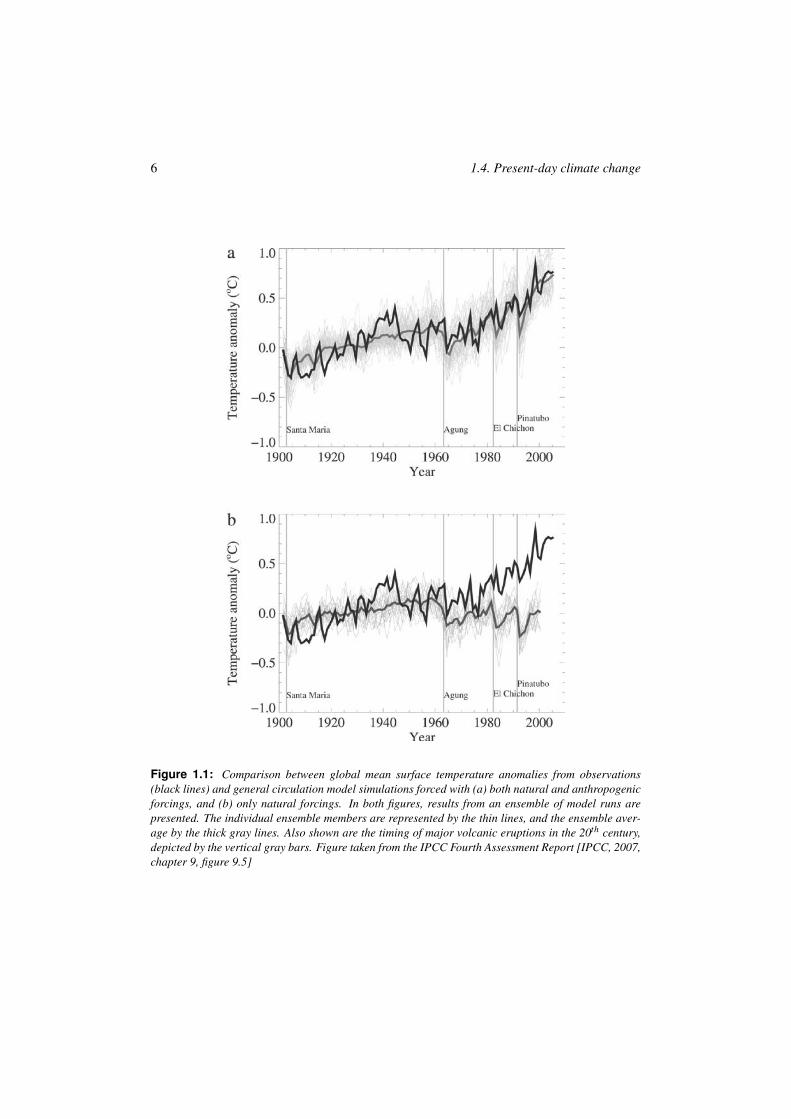
Up until the industrial revolution about 200 years ago, we can be certain that variations in cli-mate had natural causes. Combustion of fossil fuels has since then led to an unprecedentedlyrapid increase in atmospheric concentrations of carbon dioxide (CO2) and other greenhousegases like methane (CH4). Atmospheric CO2 concentrations have increased from 280 ppm inthe pre-industrial era (1000–1750 AD) to 388 ppm in 2008, an increase of almost 40%. Asgreenhouse gases are transparent to solar radiation but opaque for heat emitted by the Earth,it won’t be difficult to understand that the observed recent warming at the Earth’s surface isvery likely due to anthropogenic emissions of greenhouse gases, in line with findings fromthe most recent assessment of the Intergovernmental Panel for Climate Change [IPCC, 2007].In an interesting modelling experiment, the evolution of global climate during the last centuryis simulated with and without forcing from anthropogenic emission of greenhouse gases andaerosols. Figure 1.1, containing the results of this experiment, convincingly shows that cur-rent global warming (1950 to present) can no longer be explained by natural climate variabil-ity [IPCC, 2007]: beyond 1950, the model runs that do not take into account anthropogenicforcings start to deviate significantly from the observed globally-averaged temperature trend.
6 1.4. Present-day climate change
Figure 1.1: Comparison between global mean surface temperature anomalies from observations(black lines) and general circulation model simulations forced with (a) both natural and anthropogenicforcings, and (b) only natural forcings. In both figures, results from an ensemble of model runs arepresented. The individual ensemble members are represented by the thin lines, and the ensemble aver-age by the thick gray lines. Also shown are the timing of major volcanic eruptions in the 20th century,depicted by the vertical gray bars. Figure taken from the IPCC Fourth Assessment Report [IPCC, 2007,chapter 9, figure 9.5]
1. Snow, ice and climate 7
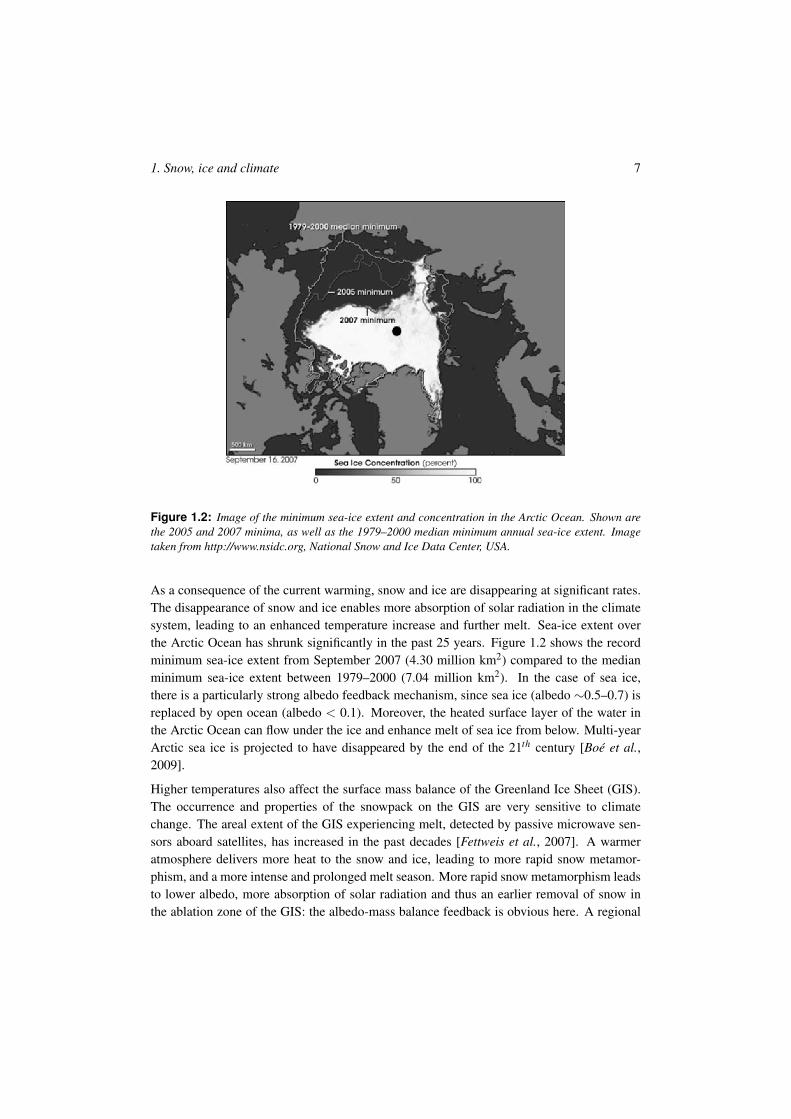
Figure 1.2: Image of the minimum sea-ice extent and concentration in the Arctic Ocean. Shown arethe 2005 and 2007 minima, as well as the 1979–2000 median minimum annual sea-ice extent. Imagetaken from http://www.nsidc.org, National Snow and Ice Data Center, USA.
As a consequence of the current warming, snow and ice are disappearing at significant rates.The disappearance of snow and ice enables more absorption of solar radiation in the climatesystem, leading to an enhanced temperature increase and further melt. Sea-ice extent overthe Arctic Ocean has shrunk significantly in the past 25 years. Figure 1.2 shows the recordminimum sea-ice extent from September 2007 (4.30 million km2) compared to the medianminimum sea-ice extent between 1979–2000 (7.04 million km2). In the case of sea ice,there is a particularly strong albedo feedback mechanism, since sea ice (albedo $0.5–0.7) isreplaced by open ocean (albedo < 0.1). Moreover, the heated surface layer of the water inthe Arctic Ocean can flow under the ice and enhance melt of sea ice from below. Multi-yearArctic sea ice is projected to have disappeared by the end of the 21th century [Boe et al.,2009].
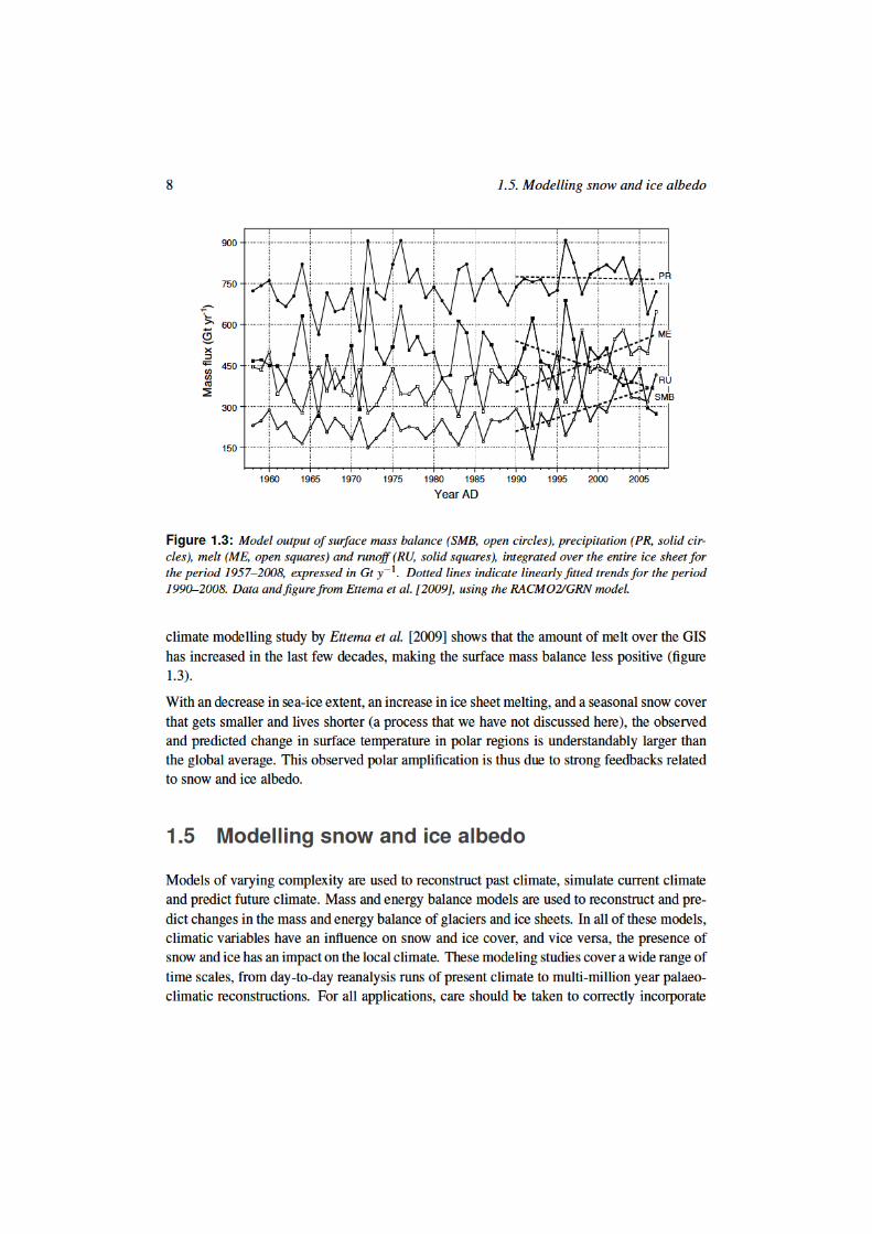
Higher temperatures also affect the surface mass balance of the Greenland Ice Sheet (GIS).The occurrence and properties of the snowpack on the GIS are very sensitive to climatechange. The areal extent of the GIS experiencing melt, detected by passive microwave sen-sors aboard satellites, has increased in the past decades [Fettweis et al., 2007]. A warmeratmosphere delivers more heat to the snow and ice, leading to more rapid snow metamor-phism, and a more intense and prolonged melt season. More rapid snow metamorphism leadsto lower albedo, more absorption of solar radiation and thus an earlier removal of snow inthe ablation zone of the GIS: the albedo-mass balance feedback is obvious here. A regional
10 1.6. The Summit Radiation Experiment (SURE ’07)
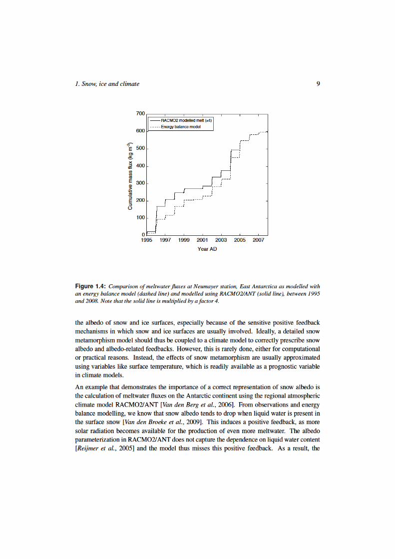
estimate of meltwater production will be too small at locations where surface temperatureexceeds the melting point. In figure 1.4, it is shown that at Neumayer station, a coastal stationin East Antarctica, meltwater production computed by RACMO2/ANT is underestimated bya factor of 4 [Van den Broeke et al., 2009].
In an increasing number of studies, global or regional climate models are coupled to an icesheet model in order to study the effects of climate change on ice sheets, and to assess therole of ice sheets in climate. Furthermore, regional climate models are employed to computeenergy and mass balance histories of ice sheets. A potential problem in these applications isthat the model grid resolution hardly exceeds the typical width of the ablation zone of an icesheet, which is in the order of a few tens of kilometres. The albedo-mass balance feedbackis likely to be poorly captured. For sea ice, the correct representation of positive feedbackmechanisms is challenged in a similar fashion, due to low grid resolution. However, theseproblems are not addressed in this thesis.
Improvement of snow and ice albedo representations in models requires a good knowledgeof the processes that influence albedo. Improving knowledge about snow and ice albedo, andabout the interaction between solar radiation and snow and ice surfaces in general, is the mainmotivation for the research presented in this thesis. In this thesis, I will combine a model forthe albedo of snow with measurements from several locations in Greenland and Antarctica.In the summer of 2007, an experiment dedicated to the radiation and energy budget of polarsnow was carried out in Greenland, from which results are used in this thesis. A summary ofthis experiment is given in the next section.
1.6 The Summit Radiation Experiment (SURE ’07)
In chapters 6 and 7, results from the Summit Radiation Experiment (SURE ’07) are analyzedand presented. This glaciometeorological experiment was set up in order to get more insightinto the radiation and energy balance of a polar ice sheet surface. In particular, the influenceof snow microstructure on the optical properties of the snowpack was studied, as well as therole of solar radiation and albedo in the energy budget of the snowpack.
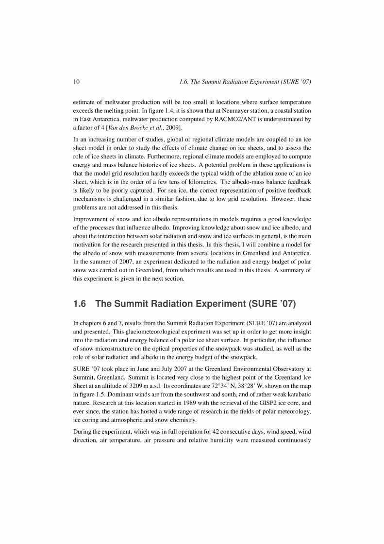
SURE ’07 took place in June and July 2007 at the Greenland Environmental Observatory atSummit, Greenland. Summit is located very close to the highest point of the Greenland IceSheet at an altitude of 3209 m a.s.l. Its coordinates are 72#34’ N, 38#28’ W, shown on the mapin figure 1.5. Dominant winds are from the southwest and south, and of rather weak katabaticnature. Research at this location started in 1989 with the retrieval of the GISP2 ice core, andever since, the station has hosted a wide range of research in the fields of polar meteorology,ice coring and atmospheric and snow chemistry.
During the experiment, which was in full operation for 42 consecutive days, wind speed, winddirection, air temperature, air pressure and relative humidity were measured continuously
12 1.6. The Summit Radiation Experiment (SURE ’07)
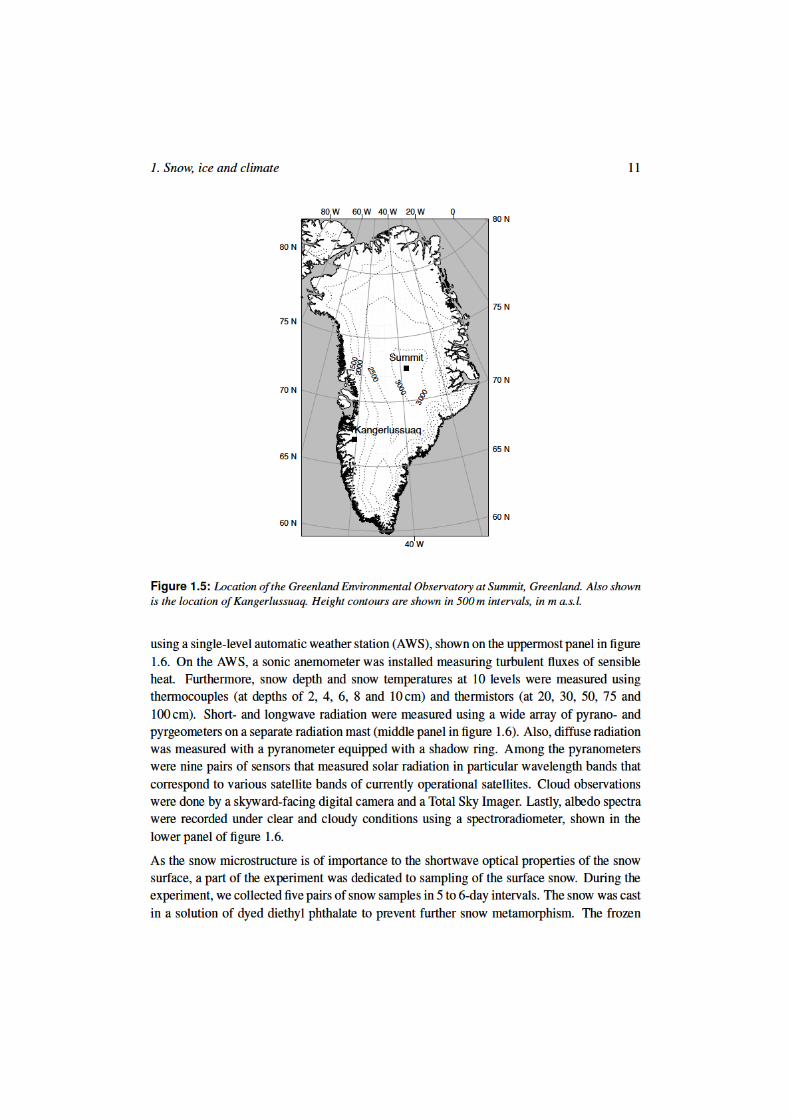
Figure 1.6: Top: The automatic weather station deployed during SURE ’07 (Young = wind speed anddirection monitor, CNR1 = shortwave and longwave radiation, Vaisala PTU = temperature, pressureand humidity, Sonic = sonic anemometer). Middle: Radiation setup (CM21 = shortwave radiation,CG4 = longwave radiation, CM11 (9%) = narrowband pyranometers, Eppley PIR2 = incoming long-wave radiation, Hukseflux = short- and longwave radiation, CNR1 = short- and longwave radiation).The inset shows a setup for diffuse radiation using a CM21 pyranometer and a shadow ring. Bottom:Spectroradiometer setup.
1. Snow, ice and climate 13
samples were transported to the cold laboratory of the Institute for Snow and AvalancheResearch in Davos, Switzerland, and cut into thin slices. Applying stereological methods todigital photographs of these sections yields a measure for snow grain size in the snowpack.
1.7 This thesis
In this thesis, radiative transfer modelling in the atmosphere and the snowpack has beencombined with field observations to learn more about the role of snow, ice and clouds in thesolar radiation budget of glaciers and ice sheets.
In chapter 2, a radiative transfer model is introduced for accurate computation of shortwaveradiative transfer in the snow-atmosphere system. The originally monochromatic model ismodified for calculations in the entire solar spectrum using the so-called correlated-k tech-nique. The details of this model adaptation are documented in this chapter, and the broadbandradiative transfer model is validated using both a model intercomparison and a comparisonbetween model calculations and observations of solar radiation made in Cabauw, The Nether-lands.
Chapter 3 describes how the model presented in the previous chapter is extended with thepossibility to include snow and cloud layers. In a series of model experiments, the influ-ence on snow characteristics, solar elevation, and clouds on the albedo of a snow surface isdemonstrated.
In chapter 4, the model presented in chapters 2 and 3 is applied to solar radiation data thatwere collected by automatic weather stations in Antarctica between 1998 and 2001. Usingthe radiative transfer model, the attribution of several processes to variations in snow surfacealbedo is investigated.
Clouds have a considerable impact on the radiation balance of the snow surface, depending ontheir optical thickness. Using concurrent observations of incoming solar radiation and albedofrom different measurement locations in Greenland and Antarctica, a technique to retrievecloud optical thickness is presented in chapter 5.
Chapter 6 deals with the energy budget of the snowpack, particularly focusing on solarradiation that penetrates into the snow and causes subsurface heating as it is absorbed belowthe surface. Meteorological and radiation observations made during SURE ’07 are used in amodel that reconstructs the energy budget of the snow. Radiative transfer model calculationsare used to investigate the role of radiation penetration.
This thesis is concluded with chapter 7, in which concurrent observations of the structureand spectral albedo of the snow surface during SURE ’07 are combined and compared tomodel calculations. This chapter shows the effect of the structure of the uppermost snowlayer on the optical properties of the snowpack.

2Broadband radiative transfer
Summary
Using the correlated k-distribution method for gaseous absorption, the originally monochro-matic doubling-adding radiative transfer model DAK (Doubling Adding KNMI) has beenadapted for calculations of broadband atmospheric radiative transfer. The model can nowcalculate the solar broadband irradiances reflected and transmitted by the atmosphere, aswell as the internal irradiances within the atmosphere. In a model intercomparison study,DAK broadband diffuse and direct irradiances agree well with results from the parameter-ized radiative transfer model SMARTS (Simple Model for Atmospheric Radiative Transferof Sunshine). Agreement is best for a purely Rayleigh-scattering atmosphere, with maximum1% difference for direct irradiance, and 3.5% for diffuse irradiance. In an atmosphere con-taining aerosols, model difference is less than 1% for direct irradiance, but slightly larger fordiffuse irradiance (approximately 6%), presumably due to the parameterization in SMARTS.It is very important to treat the aerosol optical properties dependent on wavelength in DAK.By doing so in a radiative closure study at the site of Cabauw, The Netherlands, excellent clo-sure was obtained for 72 cases of clear-sky global (+0.3% mean deviation), direct (+0.8%)and diffuse (+0.2%) irradiance.
This chapter is based on (1) Kuipers Munneke, P., C. H. Reijmer, M. R. van den Broeke, P. Stammes, G. Konig-Langlo and W. H. Knap (2008), Analysis of clear-sky Antarctic snow albedo using observations and radiative transfermodeling, J. Geophys. Res. (D), 113, D17,118, doi:10.1029/2007JD009653. (2) Wang, P., W. H. Knap , P. KuipersMunneke and P. Stammes (2008), Clear-sky atmospheric radiative transfer: a model intercomparison for shortwaveirradiances, in IRS 2008: Current problems in atmospheric radiation. (3) Wang, P., W. H. Knap, P. Kuipers Munnekeand P. Stammes (2009), Clear-sky shortwave radiative closure for the Cabauw Baseline Surface Radiation Networksite, the Netherlands, J. Geophys. Res. (D), 114, D14,206, doi10:1029/2009JD011978.
15
16 2.1. Introduction
2.1 Introduction
This thesis is devoted to the subject of radiative transfer of sunlight in the snow-atmospheresystem. In this chapter, we will lay out the physical framework for a model that describesradiative transfer of sunlight in a clear-sky atmosphere. This is the first important ingredientfor a proper description of radiative transfer in an atmosphere that contains clouds, and isbounded below by a snow surface.
We will start with introducing single-scattering properties of a volume element in the at-mosphere (section 2.2). As the atmosphere consists of many scatterers (particles, aerosols,clouds), we will extend the theory of single scattering to multiple scattering in section 2.3.In section 2.4, we will present the technique of doubling-adding as a numerical method tocompute multiple scattering in atmospheric radiative transfer.
The optical properties of the atmosphere differ widely for different wavelengths. For a properdescription of broadband solar radiation in the snow-atmosphere system, it is therefore nec-essary to take into account this wavelength dependence. The doubling-adding method istherefore extended with the correlated-k method for the efficient computation of broadbandradiative transfer of sunlight in the atmosphere. This is treated in section 2.5. The implemen-tation of the correlated-k method is verified in a model intercomparison (section 2.6) and aradiative closure study, using observations from a site in The Netherlands during a period ofclear-sky conditions (section 2.7).
2.2 Single scattering
First, we will define the quantities radiance and irradiance, which form the basis of thedescription of radiative transfer. Consider a radiant flux ! [W] through a surface A [m2] (seefigure 2.1). Irradiance (also called flux density) is then defined as:
E = d!/dA (2.1)
in [W m"2]. Spectral irradiance is the irradiance between wavelength " [nm] and " +d" :
E" = d2!/dAd" (2.2)
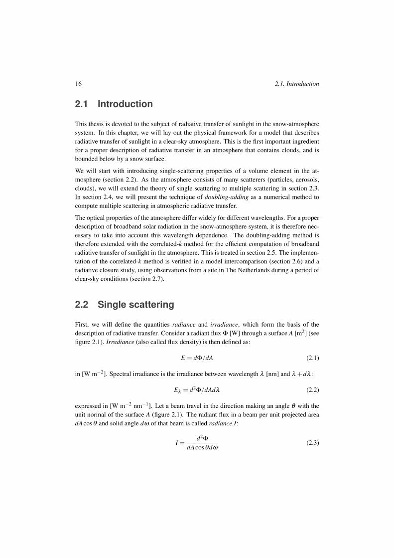
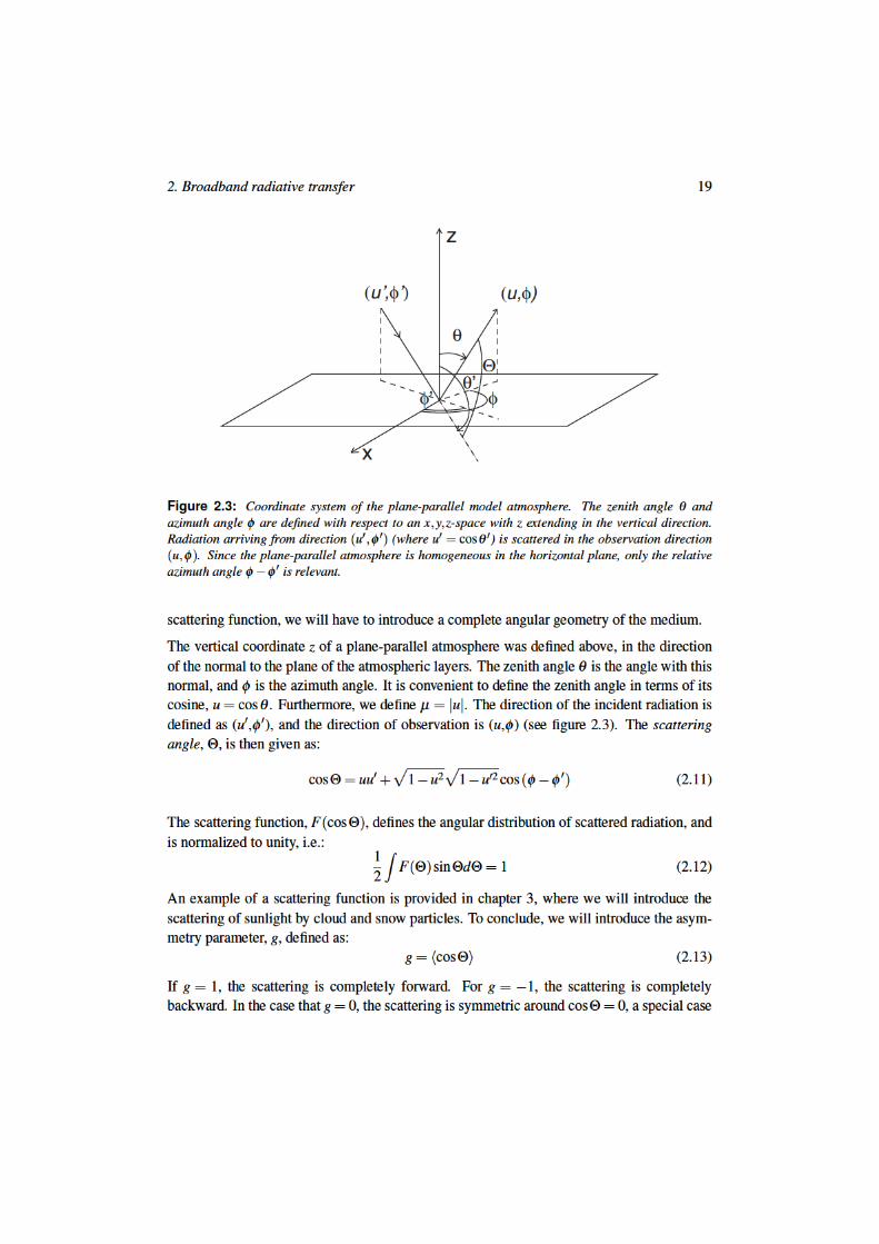
expressed in [W m"2 nm"1]. Let a beam travel in the direction making an angle # with theunit normal of the surface A (figure 2.1). The radiant flux in a beam per unit projected areadAcos# and solid angle d$ of that beam is called radiance I:
I =d2!
dAcos#d$(2.3)
20 2.3. Multiple scattering
being isotropic scattering.
2.3 Multiple scattering
In the previous section, we have developed a set of quantities with which we are able to de-scribe single-scattering processes from a volume element embedded in the atmosphere. Theatmosphere consists of numerous of these volume elements, and radiation is also scatteredbetween these volume elements. This process is called multiple scattering.
Equivalent to extinction, scattering and absorption coefficients for individual particles, we candefine the optical thickness of an atmospheric layer, b, to characterize its optical properties.Separating extinction by aerosols or cloud particles (superscript a) and molecules (superscriptm), we can write:
b = bmsca +bm
abs +basca +ba
abs (2.14)
where b is the total or extinction optical thickness, baabs and bm
abs are the absorption opticalthicknesses for aerosols and molecules, and ba
sca and bmsca the scattering optical thicknesses
for aerosols and molecules. In fact, b equals & (equation 2.10), but now for the entire layer orthe entire atmosphere. The single-scattering albedo that holds for individual particles is alsovalid for these layer properties:
$ =ba
sca +bmsca
b(2.15)
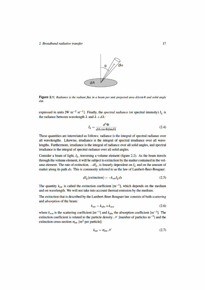
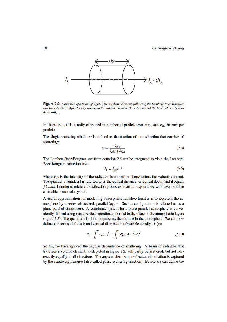
In an atmosphere, there is both loss of radiation due to scattering and absorption, and gaindue to thermal emission and multiple scattering. Of these emission processes, we will neglectthermal emission, since we consider shortwave (solar) radiation only. The total change inradiation is:
dI" = dI" (extinction)+dI" (emission) ="kextds(I" " J" ) (2.16)
where J" is a source function for emission. Since ds is in the traveling direction of radiation,thus making an angle # with the z-direction, we can use dz ="uds to get:
dI" ="kextdz"u
(I" " J" ) (2.17)
and, employing the relation d& ="kextdz:
udI"d&
="I" + J" (2.18)
Both I" and J" depend on (&,u,'). Equation 2.18 is the time-independent radiative transferequation (RTE) for a plane-parallel atmosphere. This equation is valid if radiative fluxes are
2. Broadband radiative transfer 21
stationary, and changes in the properties of the medium are sufficiently slow. In planetaryradiative transfer problems, these conditions are easily met.
For the particular case of a plane-parallel atmosphere that is illuminated from above withincident sunlight having spectral irradiance E"0, and without taking into account thermalemission of radiation, we can express the RTE as:
udI" (&,u,')
d&= "I" (&,u,')
+$4(
" 2(
0
" 1
"1F(&,u,u&,' "' &)I" (&,u&,' &)du&d' & (2.19)
+$4(
F(&,u,u0,' "'0)e"&/µ0 E"0
where (u0,'0) is the direction of the incident sunlight. The source function J contributingto the direction (u,') consists of (1) radiation that is scattered from all directions (u&,' &),which is the second term on the right-hand side of equation 2.19, and (2) the scattering of theattenuated solar source e"&/µ0E"0, which is the third term on the right-hand side.
The RTE is presented here as a conservation law. Its derivation as sketched above is ratherphenomenological, and it does not explain why or how particles are scattered. In otherwords, the physical basis of this derivation is uncertain. Only recently, the RTE has beenderived from a unified microphysical approach, evolving directly from Maxwell’s equationsfor macroscopic electromagnetic scattering [Mishchenko et al., 2006; Mishchenko, 2008].These papers discuss elastic scattering of electromagnetic waves by random many-particlegroups, and show that the RTE is rooted in Maxwell’s equations, thereby providing a solidphysical understanding of radiative transfer in particulate media.
2.4 Doubling-adding method
Solving the RTE (equation 2.18) analytically is only possible under rather strict assumptions[see e.g. Thomas and Stamnes, 1999; Liou, 2002]. Under more complex conditions, and fullyaccounting for multiple scattering processes (as in equation 2.19), the RTE can only be solvedusing numerical methods. Various mathematical techniques have been developed to provide aformal solution of the RTE. One of these methods, which was first developed by Van de Hulst[1963], is the technique of doubling-adding. In fact, the doubling-adding method is not baseddirectly on the RTE, but it is an intuitive, physical approach to calculate multiple scattering.The starting point for doubling-adding calculations of multiple scattering is a very thin layer,the reflection and transmission of which can be computed analytically from single and dou-ble scattering theory (requiring b, $ and F(#)). This thin layer is then doubled repeatedlyuntil the desired optical thickness of the layer is reached. At each ‘doubling’ step, the inter-nal radiation field is calculated at the layer boundaries, both in downward (D) and upward
22 2.4. Doubling-adding method
(U) directions, by computing the repeated reflections between the two layers. The doublingprocedure is repeated for each of the N atmospheric layers. Finally, the ‘adding’ procedure,which is the same as the doubling procedure but for layers with different optical properties,is invoked to combine these layers to compute the radiation field of the entire atmosphere.The diffuse downward field at the lowermost boundary is the transmission function T and thediffuse upward field at the upper boundary is the reflection function R.
The model for the research in this thesis is based on the DAK model (Doubling AddingKNMI), version 2.5.1 (2005). Its mathematical foundations and numerical approach are de-scribed in De Haan et al. [1987]; Stammes et al. [1989]; Hovenier et al. [2004]. In DAK, aplane-parallel atmosphere consisting of molecules and particles (aerosols, cloud droplets orice crystals) is considered. This atmosphere is illuminated from above by a parallel beam ofmonochromatic, unpolarized solar radiation E"0 traveling in direction (µ0,'0), where µ0 )= 0.The atmosphere is bounded below by a reflecting surface with surface albedo !(" ). Inho-mogeneity of the atmosphere is approximated by a stack of N homogeneous layers. DAKcomputes the polarized internal radiation field of the atmosphere. Emission of solar radiationby the atmosphere is not considered, i.e. it is assumed that there are no internal radiationsources in the shortwave spectrum [Stammes et al., 1989].
The DAK model is capable of taking into account full polarization of radiation. We neglectpolarization in this thesis, and we will therefore not use the matrix notation encounteredin all literature on polarized doubling-adding [De Haan et al., 1987; Stammes et al., 1989;Stammes, 2001; Hovenier et al., 2004] for which DAK is regularly used. For comparisonhowever, we briefly show how the scalar quantities in this thesis are related to the matrixquantities in full polarized radiative transfer. In that case, I (omitting the subscript " ) is thefirst element of the Stokes vector I = [I,Q,U ,V ], where Q and U describe linear polariza-tion, and V represents circular polarization [Chandrasekhar, 1950]. The internal radiationfield is then described by the 4%4-matrices R, T, U and D. These correspond to R, T , Uand D in this thesis. The scattering function F(#) mentioned above is equal to the F11(#)-element of the 4%4 scattering matrix F(#), and also to the element Z11(#) of the 4%4 phasematrix Z(#) [Hovenier et al., 2004].
DAK is a 1-D model in the sense that the spatial coordinate in the vertical direction is the onlyone considered: it describes a plane-parallel atmosphere, in which all properties of the layersare assumed to be homogeneous in the horizontal directions. At each model layer however,the radiation field is computed three-dimensionally — as a function of zenith and azimuthangles # and ' .
In DAK, the scattering function F(#) is specified for molecular (Fm(#)) and aerosol or cloudparticles (Fa(#)) scattering. The computation of Fa(#) for cloud particles (water dropletsor ice crystals), is explained in section 3.2.
Molecular scattering (bmsca) in DAK is confined to elastic Rayleigh scattering, which depends
strongly on wavelength and air density [Stam et al., 2000]. Aerosol scattering and absorption
2. Broadband radiative transfer 23
bmsca and bm
abs are prescribed in DAK. Molecular absorption bmabs is a function of the absorption
cross sections of the gases in the atmosphere, which are strongly dependent on wavelength,pressure, and temperature. The calculation of bm
abs is central in the correlated-k method forbroadband calculations, which is treated in section 2.5.
2.5 Correlated k-distribution method
DAK originally is a monochromatic radiative transfer model: it calculates the internal ra-diation field at a single wavelength only. All parameters determining the radiation field inthe atmosphere can vary strongly with wavelength, e.g. the surface albedo !(" ), molecularscattering bm
sca(" ), and most importantly, absorption by gas molecules, represented by themolecular absorption optical thickness bm
abs(" ). The latter is also dependent on the tempera-ture and pressure of the gases constituting the atmosphere. If the entire shortwave spectrum(250 < " < 4000 nm) is to be analyzed at a resolution sufficient to capture the irregularpatterns of gas absorption bands, it would require several thousands of monochromatic line-by-line calculations. To avoid this computationally costly approach, we have implementedthe correlated k-distribution method for gaseous absorption in DAK.
The correlated k-distribution allows for the computation of gas absorption of an entire wave-length interval using only a few radiative transfer calculations. The key aspect of the k-distribution method is to rearrange the absorption cross-sections in a wavelength interval inorder of increasing magnitude, instead of by wavelength. In order to make this arrangementvalid, the scattering properties of the atmosphere are assumed to be constant over the wave-length interval. Mathematically, this can be elucidated as follows:
Consider the direct transmission T ()) in a wavelength interval $" (Lambert-Beer-Bouguerextinction law):
T ()) =1
$"
"
$"e"k(" )) d" , (2.20)
where ) is the column density [number of absorbing particles m"2] along the path of the lightbeam, and k(" ) the absorption cross-section [m2 per particle]. For a slant path, ) is the slantcolumn density; for a vertical path, ) is the vertical column density. Note that k(" ) has theunit [m2] like %ext in equation 2.7, while the coefficients kext , ksca and kabs used in section 2.2have the unit [m"1]. Although we could have chosen a different symbol for k(" ) for clarity,we have decided to follow closely the notation in correlated-k literature. With this notation,the absorption optical thickness bm
abs(" ) is given by bmabs(" ) = k(" )) , where ) is the vertical
column density.
As mentioned above, the integrand in equation (2.20) is highly irregular due to the complexpattern of absorption lines as a function of wavelength. It is now possible to rearrange theabsorption cross sections without changing the integral in equation 2.20. If we define the
24 2.5. Correlated k-distribution method
distribution function f (k), being the probability of occurrence of a specific value of k in thewavelength interval $" , the transmission in that wavelength interval becomes:
T ()) =" "
0f (k)e"k) dk (2.21)
The integrand is no longer dependent on wavelength " . Mathematically, the quintessenceof the k-distribution method is to turn this integrand into a smooth function by reorderingthe absorption cross-sections k in order of increasing magnitude, and defining the cumulativeprobability function g(k) [see Lacis and Oinas, 1991]:
g(k) =" k
0f (k&)dk& (2.22)
Upon inversion of g(k), we get
T ()) =" 1
0e"k(g)) dg. (2.23)
Since the integrand in equation (2.23) is now a smooth function in g-space by definition, theintegral of equation (2.23) can be adequately approximated by a numerical Gaussian quadra-ture method involving only a few (typically 5-16) quadrature points, i.e. monochromaticradiative transfer calculations. In a formula, this Gaussian integral approximation becomes
T ()) =n
%j=1
a je"k(g j)) (2.24)
which is a summation over n Gaussian quadrature points, using absorption cross-sections kat coordinate g j, and their corresponding weights a j.
By using the same Gaussian quadrature for every atmospheric layer, the k-distribution methodis said to be ‘correlated’. The interested reader is referred to the overview given by Thomasand Stamnes [1999, Ch. 10] for a thorough mathematical treatment.
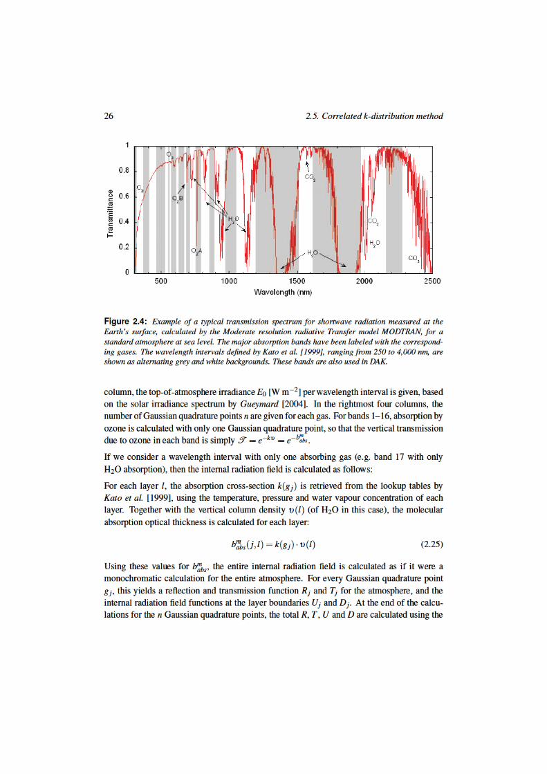
The determination of all k(g j) and a j does initially require many line-by-line calculations foreach wavelength interval. This has been done by Kato et al. [1999] using the HITRAN 1992database. The correlated-k absorption cross-sections are available through the libRadtransoftware package (http://www.libradtran.org). Kato et al. [1999] subdivided the shortwavespectrum into 32 wavelength intervals that closely follow absorption bands of the gases CO2,O2, O3 and H2O. These wavelength intervals are shown in an example transmission spectrumin figure 2.4. For each gas in each wavelength interval, Kato et al. [1999] generated lookuptables of absorption cross-sections k as a function of temperature and pressure, for each Gaus-sian quadrature point. The absorption cross-sections of water vapour are also dependent onthe water vapour concentration itself.
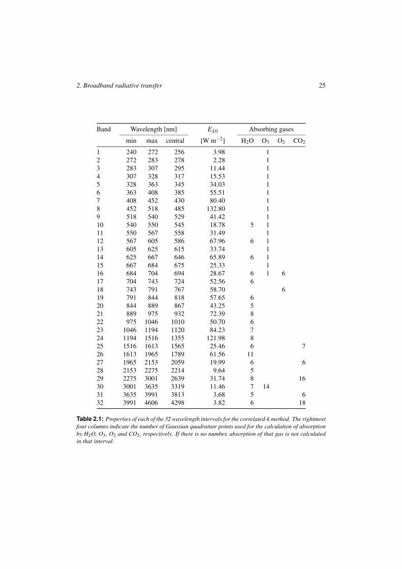
In table 2.1, we present the 32 wavelength intervals of the correlated-k method. In the fourth
2. Broadband radiative transfer 25
Band Wavelength [nm] E"0 Absorbing gases
min max central [W m"2] H2O O3 O2 CO2
1 240 272 256 3.98 12 272 283 278 2.28 13 283 307 295 11.44 14 307 328 317 15.53 15 328 363 345 34.03 16 363 408 385 55.51 17 408 452 430 80.40 18 452 518 485 132.80 19 518 540 529 41.42 110 540 550 545 18.78 5 111 550 567 558 31.49 112 567 605 586 67.96 6 113 605 625 615 33.74 114 625 667 646 65.89 6 115 667 684 675 25.33 116 684 704 694 28.67 6 1 617 704 743 724 52.56 618 743 791 767 58.70 619 791 844 818 57.65 620 844 889 867 43.25 521 889 975 932 72.39 822 975 1046 1010 50.70 623 1046 1194 1120 84.23 724 1194 1516 1355 121.98 825 1516 1613 1565 25.46 6 726 1613 1965 1789 61.56 1127 1965 2153 2059 19.99 6 628 2153 2275 2214 9.64 529 2275 3001 2639 31.74 8 1630 3001 3635 3319 11.46 7 1431 3635 3991 3813 3.68 5 632 3991 4606 4298 3.82 6 18
Table 2.1: Properties of each of the 32 wavelength intervals for the correlated-k method. The rightmostfour columns indicate the number of Gaussian quadrature points used for the calculation of absorptionby H2O, O3, O2 and CO2, respectively. If there is no number, absorption of that gas is not calculatedin that interval.

2. Broadband radiative transfer 27
weights a j:
R =n
%j=1
a jR j (2.26)
T =n
%j=1
a jTj (2.27)
U =n
%j=1
a jUj (2.28)
D =n
%j=1
a jD j (2.29)
In some bands, radiation is absorbed by more than one gas species (e.g. band 25 with bothH2O and CO2 absorption). Assuming that absorption by two different species is uncorrelated[Kato et al., 1999], the molecular absorption optical thickness is calculated for each layer as:
bmabs( j1, j2, l) = k(g1, j1))1(l)+ k(g2, j2))2(l) (2.30)
where subscripts 1 and 2 denote the two gas species. If there are n1 and n2 Gaussian quadra-ture points for species 1 and 2, there will be n1 · n2 calculations of the internal radiationfield for that wavelength interval. The resulting reflection R for the wavelength interval iscalculated as:
R =n1
%j1
n2
%j2
a1, j1 a2, j2R j1 j2 (2.31)
and similarly, T , U and D are computed. In general, for p overlapping gases,
R =n1
%j1
n2
%j2
. . .np
%jp
$R j1 j2... jp
$p
&q=1
aq, jq
%%(2.32)
and again, similar relations hold for T , U and D. In equations 2.31 and 2.32, R j1 j2 andR j1 j2... jp are in fact similar to R j in equation 2.27, but with multiple subscripts for the differentgases.
In the correlated-k distribution method implemented in DAK, all other properties of the atmo-sphere and surface, e.g. molecular (Rayleigh) scattering, are taken at the central wavelengthof each wavelength interval (see table 2.1).
28 2.6. Validation I: Model intercomparison
2.6 Validation I: Model intercomparison
The radiative transfer model outlined in sections 2.4 and 2.5 needs a proper validation beforeit is applied to radiative transfer studies in the snow-atmosphere system. Although an obviousvalidation setup would be to compare model output to a ‘laboratory’ setting in which allrelevant parameters are accurately known, radiative transfer in the atmosphere is not easilycaptured in such a laboratory environment. As a surrogate, we will present a comparisonof DAK with another radiative transfer model in this section, and a radiative closure study insection 2.7. The aim of the model intercomparison is to put certain confidence in the output ofDAK, although an intercomparison study can never prove model correctness — after all, bothmodels could be equally wrong yet show excellent agreement. The radiative closure study insection 2.7 however, serves two important purposes. First of all, it is meant to demonstratethe ability of the model to simulate atmospheric radiative transfer (but again, not prove modelcorrectness). Secondly, a very important implication of good closure results is that we candescribe radiative transfer in a real atmosphere with the processes that are included in themodel, and therefore understand all processes in atmospheric radiative transfer.
In this section, we subject the broadband version of DAK to a comparison with the parameter-ized radiative transfer model SMARTS (Simple Model for Atmospheric Radiative Transfer ofSunshine, [Gueymard, 2001]), also documented in Wang et al. [2008]. SMARTS deploys pa-rameterizations that are based on calculations with the Moderate resolution radiative Transfermodel MODTRAN [Berk et al., 1998]. In a publication by Michalsky et al. [2006], SMARTSis one of the models that was used in an attempt to attain radiative closure for direct and dif-fuse shortwave radiation under clear-sky conditions during a large aerosol intensive observa-tion period at the Southern Great Plains site (near Billings, Oklahoma, United States) in May2003. It was found that direct-beam calculations by SMARTS were accurate to within 0.1%,whereas diffuse radiation calculations differed by 1.9% on average. This result is within theestimated uncertainty of the direct (8–12%) and diffuse (4%) irradiance measurements andmuch better than previous clear-sky closure studies.
For the clear-sky irradiance model intercomparison between DAK and SMARTS, the inputwas prepared identically for both models. The atmospheric profile is a standard mid-latitudesummer atmosphere, describing vertical profiles of temperature, pressure, H2O, O3, and O2.The CO2 mixing ratio was set at 370 ppmV, well-mixed throughout the atmosphere. Thesolar spectrum was adopted from the SMARTS model [Gueymard, 2004], adding up to atotal solar irradiance at the top-of-atmosphere of 1366 W m"2, perpendicular to the beam.The SMARTS model computed irradiances for solar zenith angles between 0# and 90# withintervals of 1#, while DAK calculations were done at 0, 30, 45, 60, 70 and 80# for compu-tational reasons. The results of this comparison are shown in figure 2.5, showing DAK andSMARTS direct, diffuse and global irradiances in panel (a) and their differences in panel (b).Global irradiance — also called total irradiance — is here defined as the sum of direct anddiffuse irradiances. The absolute differences in both direct and diffuse irradiance are small
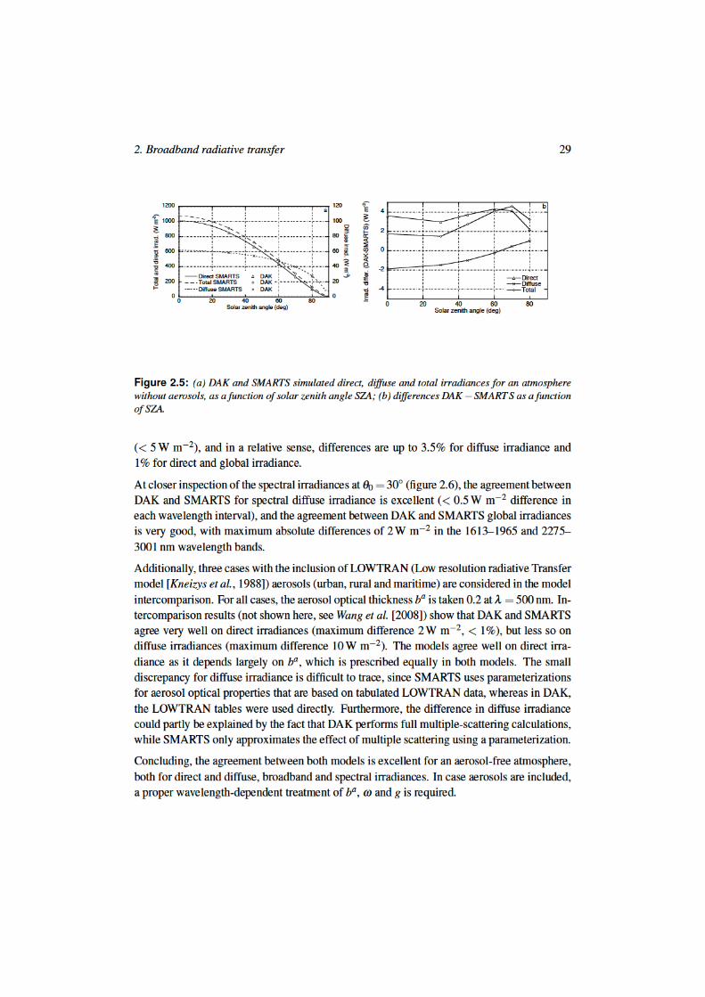
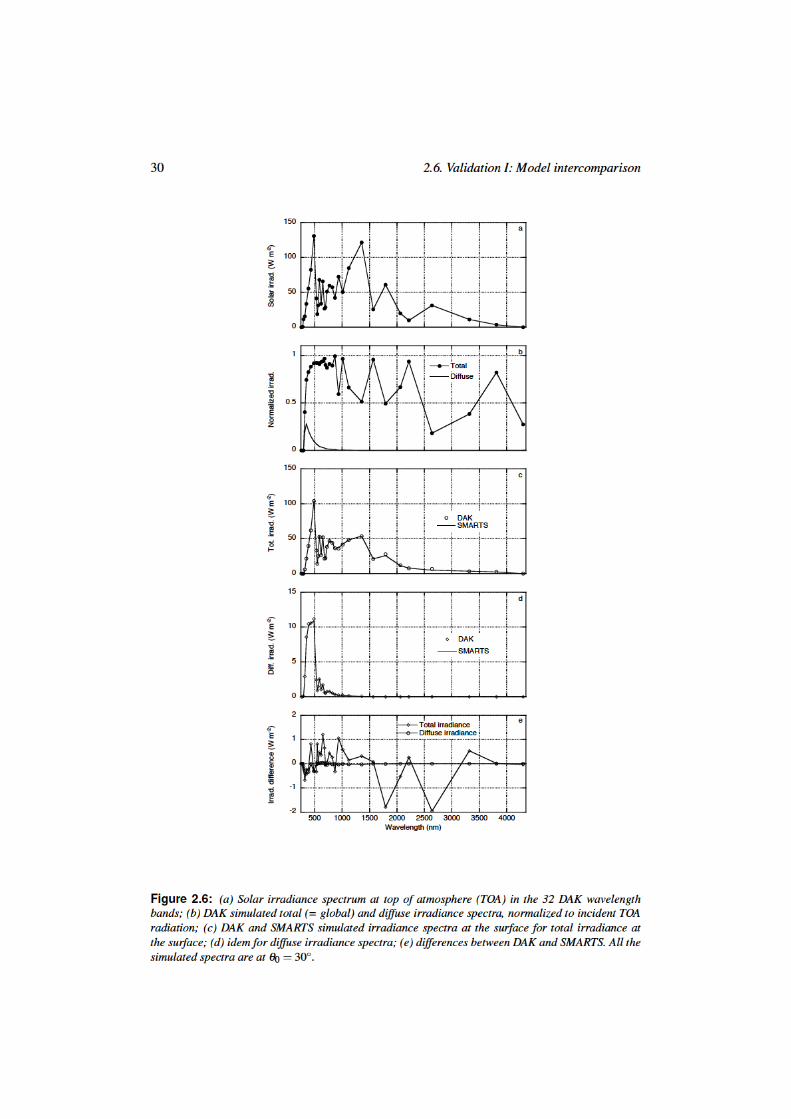
2. Broadband radiative transfer 31
2.7 Validation II: Clear-sky radiative closure study
Although the model intercomparison in section 2.6 gives confidence in the performance ofDAK, the model is put to the test by comparing model output to clear-sky measurementsof direct, diffuse and global irradiances at the surface. During the last two decades, severalattempts have been made to achieve agreement between clear-sky broadband irradiance mod-els and surface measurements of direct and diffuse irradiance [Henzing et al., 2004]. Suchan agreement is called closure. In general, models and measurements agreed well for thedirect component, but agreement for diffuse irradiances remained problematic. Due to im-proved instrumentation and model input specification, Michalsky et al. [2006] were able topresent better results than previously achieved. The authors report biases between modelsand measurements of generally less than 1% for direct irradiance and less than 1.9% for dif-fuse irradiance. In general, the number of studies reporting a satisfactory degree of closurefor both direct and diffuse irradiance is still limited.
For the comparison under consideration here, we deployed the measurements made at Cabauw,The Netherlands (51.97 #N, 4.93 #E), during the May 2008 IMPACT (Intensive MeasurementPeriod At the Cabauw Tower) measurement campaign, performed in the framework of EU-CAARI (European Integrated project on Aerosol Cloud Climate and Air Quality Interactions)[Wang et al., 2009]. Although IMPACT produced a wealth of data, it was decided to use onlyroutine measurements from the Baseline Surface Radiation Network (BSRN) and the AerosolRobotic Network (AERONET, [Dubovik et al., 2000]), supplemented with radiosonde obser-vations. The rationale for this approach is the possibility of performing similar closure studiesat other locations or for other periods.
In section 2.6, it was already shown that a closure study of measured and modelled shortwaveradiation would benefit from taking into account the wavelength dependence of aerosol op-tical properties. In order to prescribe appropriate aerosol optical thickness ba
tot * baabs +ba
sca,data was extracted from AERONET Level 1.5 data for Cabauw. These data are available atwavelengths of 440, 675, 870 and 1020 nm. Between 440 and 1020 nm, values for singlescattering albedo $ , asymmetry parameter g and ba
tot are interpolated to the DAK wavelengthgrid. Outside this part of the spectrum, $ and g were taken from the continental aerosolmodel of WCP-55 [Deepak and Gerber, 1983]. Outside the 440–1020 nm range, ba
tot wasextrapolated using the four AERONET values.
Temperature, pressure and humidity were taken from radiosonde launches and regridded tothe DAK vertical layer profile of 32 layers, each being 1 km thick up to a height of 25 km. Allvertical profiles of water vapour were scaled to the AERONET water vapour column. Thetotal ozone column was taken from Ozone Monitoring Instrument (OMI) retrievals. A typicalspectral albedo curve for grassland was used as a lower boundary condition.
Cabauw is a location that participates in the worldwide Baseline Surface Radiation Network(BSRN) [Ohmura et al., 1998] and measures direct, diffuse and global irradiance according
32 2.7. Validation II: Clear-sky radiative closure study
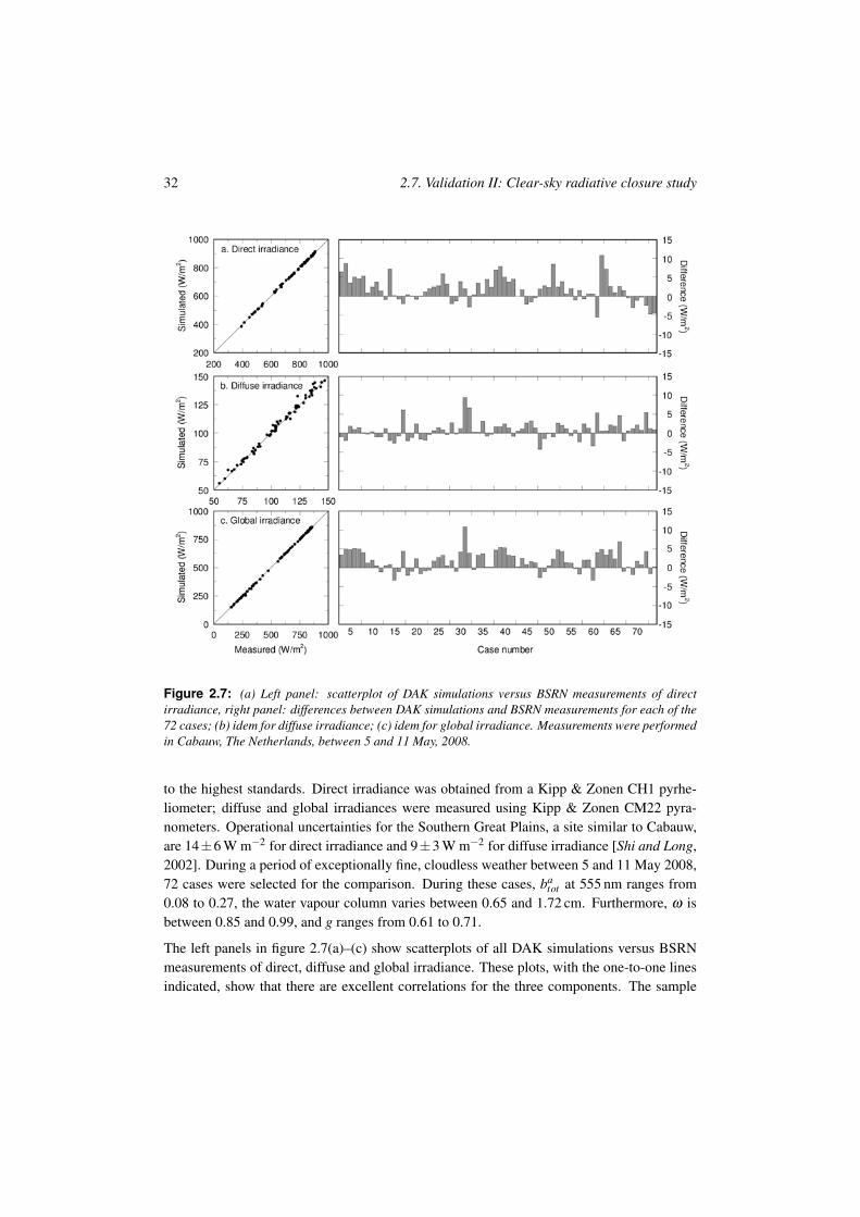
Figure 2.7: (a) Left panel: scatterplot of DAK simulations versus BSRN measurements of directirradiance, right panel: differences between DAK simulations and BSRN measurements for each of the72 cases; (b) idem for diffuse irradiance; (c) idem for global irradiance. Measurements were performedin Cabauw, The Netherlands, between 5 and 11 May, 2008.
to the highest standards. Direct irradiance was obtained from a Kipp & Zonen CH1 pyrhe-liometer; diffuse and global irradiances were measured using Kipp & Zonen CM22 pyra-nometers. Operational uncertainties for the Southern Great Plains, a site similar to Cabauw,are 14±6 W m"2 for direct irradiance and 9±3 W m"2 for diffuse irradiance [Shi and Long,2002]. During a period of exceptionally fine, cloudless weather between 5 and 11 May 2008,72 cases were selected for the comparison. During these cases, ba
tot at 555 nm ranges from0.08 to 0.27, the water vapour column varies between 0.65 and 1.72 cm. Furthermore, $ isbetween 0.85 and 0.99, and g ranges from 0.61 to 0.71.
The left panels in figure 2.7(a)–(c) show scatterplots of all DAK simulations versus BSRNmeasurements of direct, diffuse and global irradiance. These plots, with the one-to-one linesindicated, show that there are excellent correlations for the three components. The sample
2. Broadband radiative transfer 33
standard deviations are small: 3 W m"2 for direct irradiance, 2 W m"2 for diffuse irradiance,and 3 W m"2 for global irradiance. The differences between DAK simulations and BSRNmeasurements are also shown in the right panels of Figure 2.7(a)–(c). The absolute rangein model-measurement difference is between "5 and +11 W m"2 for direct irradiance, be-tween "4 and +9 W m"2 for diffuse irradiance, and between "3 and +11 W m"2 for globalirradiance. The ranges of relative differences are "1.4 to +1.6%, "3.9 to +8.5%, and "1.4to +2.7%, respectively. The mean differences are 2 W m"2 (+0.2%) for direct irradiance,1 W m"2 (+0.8%) for diffuse irradiance, and 2 W m"2 (+0.3%) for global irradiance.
The good results can partly be explained by the proper specification of the DAK model in-put and the high quality of the BSRN measurements. The simulation of direct irradianceis sensitive to values for aerosol optical properties. Since these parameters are wavelengthdependent, a correct description of their spectral behaviour is crucial for good closure results.
Considering the operational measurement uncertainties, the DAK simulations are well withinthe uncertainty range of the BSRN measurements. Even if only calibration uncertainties areconsidered, there is, on average, near-perfect agreement between the DAK simulations andBSRN measurements. Moreover, if one takes into account that the DAK simulations alsocarry a certain degree of uncertainty, the general conclusion is that excellent closure wasobtained between model and measurements of shortwave irradiances.
The strength of this closure study lies in the use of operational measurements (BSRN andAERONET), and in its relative simplicity. Around the world, 15 more BSRN stations alsoperform AERONET measurements, so the method presented here opens up possibilities formany more closure studies for different radiative and aerosol climates.
2.8 Conclusions
In this chapter, we have presented a radiative transfer model that can be used to study solarradiation in an atmosphere containing water vapour, other gases, and aerosols. Using thecorrelated-k method, we expanded the originally monochromatic DAK model into a modelfor the entire solar spectrum. The model has been compared to another radiative transfermodel (SMARTS), and to field measurements of direct, diffuse and global irradiance duringa period of clear-sky occurrence at Cabauw. Given the fact that these comparisons yieldedclose agreement of DAK with both SMARTS and the field measurements, we can be fairlycertain that the model is capable of accurately simulating radiative transfer in a clear-skyatmosphere. This is an important step towards studying the problem of radiative transfer inthe snow-atmosphere system. We will now need to incorporate, in some way, the effects ofclouds and snow on the radiation field. In the mathematical framework of the model, it meansthat we have to find a way to calculate scattering functions Fa for snow and cloud layers. Thiswill be the subject of chapter 3.

3Modelling radiative transfer in the
snow-atmosphere system
Summary
In this chapter, we demonstrate the ability of the DAK model, which was introduced in theprevious chapter, to calculate radiative transfer through clouds and within a snowpack. InDAK, clouds and snow are represented as layers with a scattering function. These scatteringfunctions are calculated using a ray tracing program that requires shape and dimensions ofan ice crystal, and a volume absorption coefficient as input. Soot in the snowpack can beincluded using scattering and absorption coefficients that are taken from the OPAC data set(Optical Properties of Aerosols and Clouds). For a clear sky over a snowpack, the effects ofsolar zenith angle, atmospheric optical thickness, and snow grain size on both spectral andbroadband snow surface albedo can be simulated adequately. Clouds increase the broadbandclear-sky albedo of snow, and annihilate the effect of solar zenith angle on broadband albedo.In the presence of clouds, the spectral albedo of snow equals that under a clear sky with asolar zenith angle of about 50#. Model results presented in this chapter agree well with resultspublished elsewhere.
The snow model has been published in Kuipers Munneke, P., C. H. Reijmer, M. R. van den Broeke, P. Stammes,G. Konig-Langlo and W. H. Knap (2008), Analysis of clear-sky Antarctic snow albedo using observations andradiative transfer modeling, J. Geophys. Res. (D), 113, D17,118, doi:10.1029/2007JD009653.
35
36 3.1. Introduction
3.1 Introduction
The clear-sky atmospheric part of the radiative transfer model DAK has been described andtested in the previous chapter. In order to perform radiative transfer calculations in and abovea snowpack, snow layers have to be included in the model. In section 3.2, we will demonstratehow optical properties of snow are defined in the model. In section 3.3, we show that themodel is able to calculate radiative transfer in the presence of a snow layer but no clouds,to which we will refer as clear-sky conditions. Several snow properties are varied and theresulting spectral and broadband surface albedos are examined.
Clouds that overlay the snowpack can also be accounted for. The optical properties of cloudsare computed in exactly the same way as those of a snowpack (section 3.2). In section 3.4,we present results of radiative transfer calculations in situations in which a cloud overlays thesnowpack.
3.2 Optical properties of snow and clouds
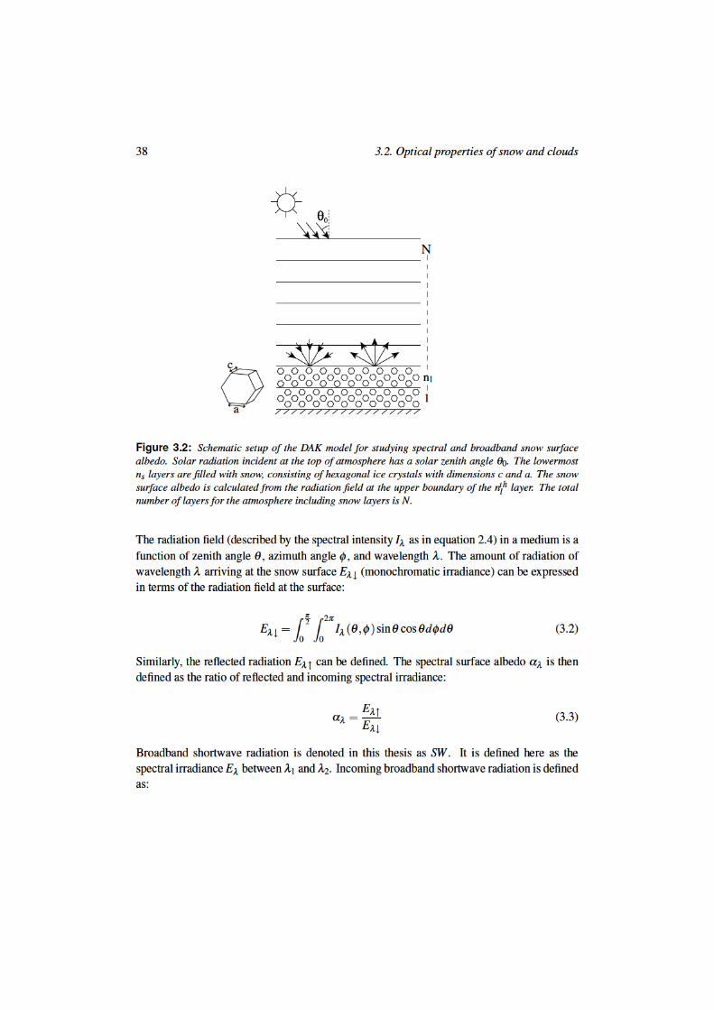
In DAK, both snow and clouds are treated as particulate media consisting of mutually inde-pendent ice crystals, or water droplet in the case of water clouds. The ice crystals can beeither of spherical or (imperfect) hexagonal shape. Water droplets attain a spherical shape.The optical properties of a snow or cloud layer are captured with a volume absorption coef-ficient ba
abs and a scattering function, Fa(#). A value for baabs is derived using the imaginary
part ' of the refractive index of ice mi [Wiscombe and Warren, 1980], updated with data fromWarren et al. [2006] for the UV/visible range:
baabs = 4(""1'(mi(" )) (3.1)
The single scattering albedo $ for a snow or cloud layer is calculated using equation 2.15,now including scattering by snow or cloud particles.
Fa(#) of the ice crystals is calculated using SPEX [Hess et al., 1998a]. SPEX is a MonteCarlo-type raytracing computer program — a large number ($107) of photons are releasedin a parallel beam from a randomly chosen initial position, and the reflections, refractionsand absorption of each photon is then computed using geometric methods. The result is thescattering function Fa(#), a function that describes the distribution of the scattered photonsover all angles. An example scattering function is shown in figure 3.1. Fa(#) is consequentlyexpanded in generalized spherical harmonics following the method by De Rooij and van derStap [1984], since these are, in a mathematical sense, easily integrated in the reflection andtransmission functions in DAK.
The scattering of solar radiation by ice crystals and water droplets typically found in cloudsand snow, is dominantly in the forward direction. Since it is numerically daunting to deal with
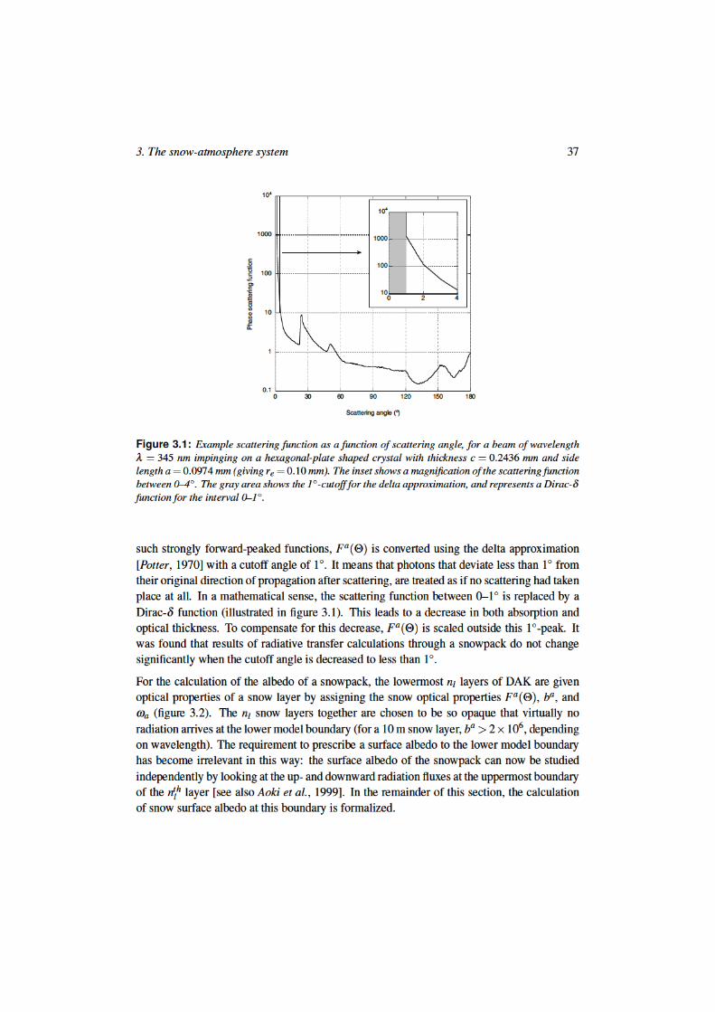
3. The snow-atmosphere system 39
SW+ =" "2
"1E"+d" (3.4)
Analogously, the reflected broadband shortwave radiation SW, is defined using E",. De-pending on the application, the values of "1 and "2 will vary a bit, but generally, they are inthe range of 250 and 4000 nm. The albedo for broadband shortwave radiation ! (hereafterreferred to as broadband albedo) is given by:
! =SW,SW+
=
! "2"1
E"+!" d"! "2
"1E"+d"
(3.5)
From the above, it is clear that the broadband albedo of the snow surface is not an inherentproperty of the snow. It depends on the radiation field arriving at the surface, which mayin turn depend on the zenith angle of the sun, the absorption and scattering by atmosphericgases, aerosols and clouds. This is exactly the reason why the atmospheric part of DAK, aspresented in chapter 2, is crucial in modelling snow surface albedo.
3.3 Clear-sky snow albedo
The first comprehensive and physically consistent model for the albedo of snow was putforward by Wiscombe and Warren [1980]. Using Mie theory for single scattering properties ofice crystals, and the delta-Eddington approximation for the description of multiple scattering,the authors demonstrated the effect of solar zenith angle (#0), snow grain size (radius re),and cloud cover on the albedo of a snow surface. Moreover, they discussed the effects ofclose packing of snow grains, and nonsphericity of snow grains. The same authors alsoexplored the effects of impurities contained in the snow on the surface albedo [Warren andWiscombe, 1980]. In the following sections (3.3.1–3.3.2, and 3.4), we will briefly present thewell-accepted theory of Wiscombe and Warren [1980] and Warren and Wiscombe [1980] andshow that DAK, with the inclusion of the snow model as illustrated in figure 3.2, mimics allof its aspects.
Throughout this chapter, the snowpack is assumed to consist of ice crystals shaped like ir-regular hexagonal plates. The aspect ratio ( (= c/2a) is fixed at 0.2, where c is the centralaxis of the plate (its ‘thickness’), and a the length of each of the sides of the hexagon (fig-ure 3.2). Irregularity refers to some distortion of the crystal faces. It is obtained by, withinlimits, changing the surface normal randomly while performing the ray-tracing calculations[see Macke et al., 1996; Hess et al., 1998a; Knap et al., 2005]. Its effect is to smoothen thescattering function Fa(#) somewhat.
40 3.3. Clear-sky snow albedo
To facilitate comparison with other literature, snow grain size will be expressed by the quan-tity re, best described as the optically equivalent snow grain size [e.g Nolin and Dozier,2000; Legagneux et al., 2006; Matzl and Schneebeli, 2006]. It refers to the radius of a spher-ical particle that has the same volume-to-surface ratio as the hexagonal ice plate. It has beenhypothesized [Wiscombe and Warren, 1980] and demonstrated [Grenfell and Warren, 1999;Neshyba et al., 2003] that the scattering and absorptive properties of any type of crystal canbe approximated by those of a spherical particle, as long as the volume-to-surface radio isconserved. In order to achieve this, the number of particles must be scaled.
Since the volume-to-surface (V/A) ratio of a sphere of radius r is r/3, the optically equivalentsnow grain radius is
re = 3VA
(3.6)
The number of spheres ns relative to the number of nonspherical particles n is
ns
n=
3V4(r3
e(3.7)
In the case of hexagonal plates [Neshyba et al., 2003], equation 3.6 becomes
re =3-
3ac4c+2
-3a
(3.8)
or, using ( (= c/2a):
re =3-
3a(4(+
-3
(3.9)
and
ns
n=
(4(+-
3)3
36((2 (3.10)
3.3.1 Pure snow
In this section, we present results of various numerical experiments simulating clear-sky con-ditions, in which the snow grain size re, and the solar zenith angle #0 are varied. All ex-periments in this section were carried out using a standard subarctic summer atmosphere[Anderson et al., 1986]. Similar results, using spherical ice particles only, have been pre-sented by Aoki et al. [1999] and Wiscombe and Warren [1980]. The difference between the

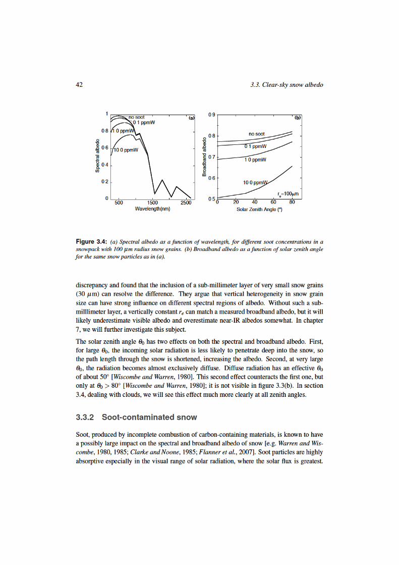

3. The snow-atmosphere system 45
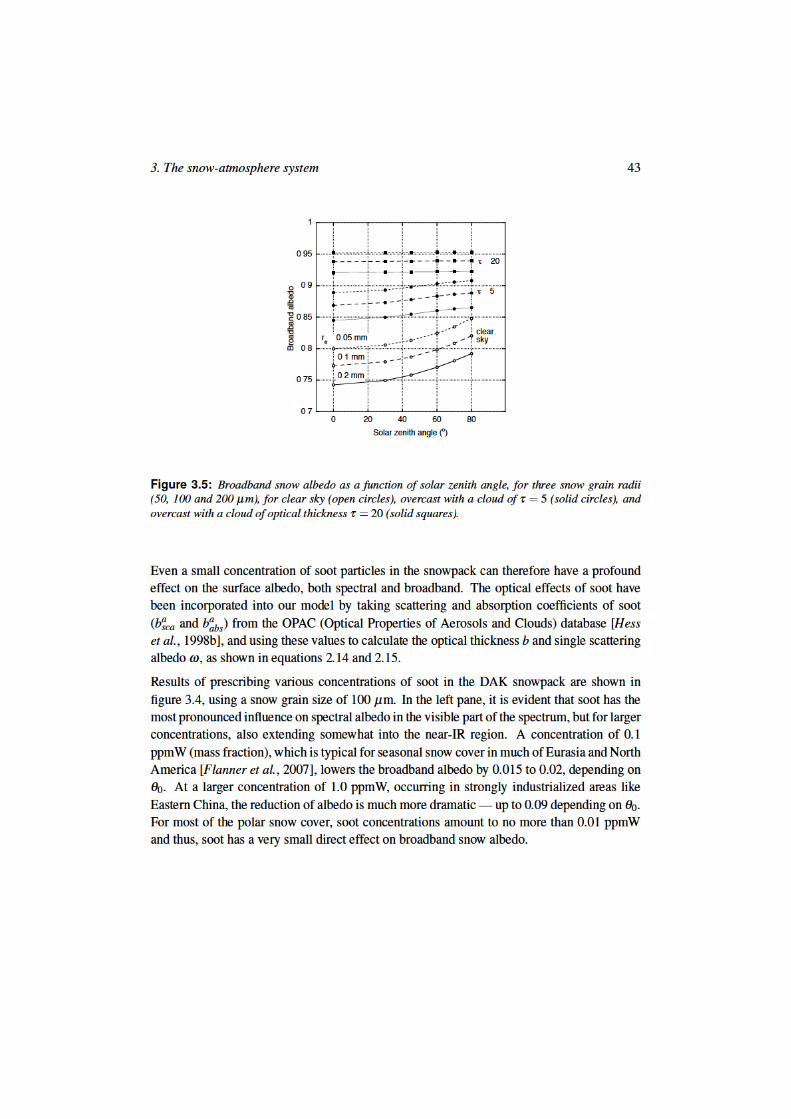
diffuse. At a given solar zenith angle, the difference between albedo for different snow grainradii also becomes somewhat smaller (see also figure 3.6). For an optically thick cloud cover,albedos can easily exceed 0.9, and even 0.95.
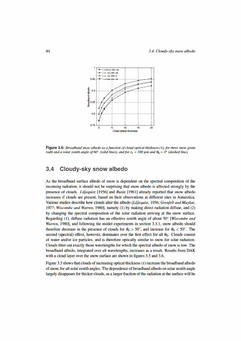
In figure 3.6, broadband snow albedo is plotted against cloud optical thickness, for a givensolar zenith angle #0 of 60# (solid lines). As cloud optical thickness increases, broadbandalbedo tends to an asymptotic value. The dashed line in figure 3.6, representing broadbandalbedo for #0 = 0#, once more illustrates that the #0-dependence of albedo vanishes as &increases.

4Analysis of clear-sky Antarctic
snow albedo
Summary
The radiative transfer model DAK has been applied to radiation data (1998–2001) fromweather stations in different climate regimes in Antarctica. The novel approach of apply-ing the model to multiple-year field data of clear-sky albedo from five locations in Dron-ning Maud Land, Antarctica, reveals that seasonal clear-sky albedo variations (0.77–0.88) aredominantly caused by strong spatial and temporal variations in snow grain size (re). Mod-elled summer season averages of re range from 22 µm on the Antarctic plateau to 64 µm onthe ice shelf. Maximum monthly values of re are 40–150% higher. Other factors influencingclear-sky broadband albedo are the seasonal cycle in solar zenith angle (at most 0.02 differ-ence in summer and spring/autumn albedo), and the spatial variation in optical thickness ofthe cloudless atmosphere (0.01 difference between ice shelves and plateau). The seasonalcycle in optical thickness of the atmosphere was found to be of minor importance (<0.005between summer and spring/autumn).
This chapter is based on Kuipers Munneke, P., C. H. Reijmer, M. R. van den Broeke, P. Stammes, G. Konig-Langlo and W. H. Knap (2008), Analysis of clear-sky Antarctic snow albedo using observations and radiative transfermodeling, J. Geophys. Res. (D), 113, D17,118, doi:10.1029/2007JD009653.
47
48 4.1. Introduction
4.1 Introduction
In chapters 2 and 3, we have presented a combined snow-atmosphere model that we can useto study spectral and broadband radiative transfer of sunlight in an atmosphere that containsabsorbing and scattering gases, clouds, and aerosols, and that is bounded below by a snowsurface. In this chapter, we will apply this model to four years of continuous field observa-tions gathered at Neumayer station, and by four automatic weather stations (AWSs) situatedat locations in various climatic regimes in Dronning Maud Land, Antarctica (see map infigure 4.1).
From these observations, we know that the broadband albedo of the snow surface ! is highlyvariable throughout the year. Despite the high values of snow albedo in Antarctica (typically0.78–0.86), the shortwave radiation balance plays a dominant role in the summer energybudget of the snow surface [e.g. Van As et al., 2005b]. The amount of absorbed shortwaveradiation, being proportional to 1"! , is very sensitive to small changes in the snow albedo.It is therefore vital to understand what factors have a strong influence on snow albedo andwhich have not. The central goal of this chapter is to identify and quantify these factors, usingthe radiative transfer model DAK. This provides a deeper understanding of the most relevantcauses of observed variations in snow albedo.
4.2 Data and methods
4.2.1 Data sets
We selected the radiation data available from five different locations in Dronning MaudLand, Antarctica. One of these locations is Station Neumayer, which has been deliveringhigh-quality, year-round measurements to the Baseline Surface Radiation Network (BSRN)[Ohmura et al., 1998] since 1994. The other four locations are automatic weather stations(AWSs) that have been collecting both radiation and meteorological data autonomously since1998 [Van den Broeke et al., 2004a].
Station Neumayer, an Antarctic base operated by Germany since 1981, is situated in DronningMaud Land (70#37’ S, 8#22’ W), on the Ekstrom Ice Shelf at 42 m above sea level (figure4.1). The Ekstrom Ice Shelf has a homogeneous and flat surface with a very small slopeupward to the south. A thorough description of the climatology of Neumayer is available inKonig-Langlo et al. [1998].
IMAU has been employing more than 10 AWSs (numbered AWS 1, 2, etc.) in Antarcticaover the past decade. We chose a set of four of these that cover distinct climatic regions inDronning Maud Land, and that have a data record of appreciable length:
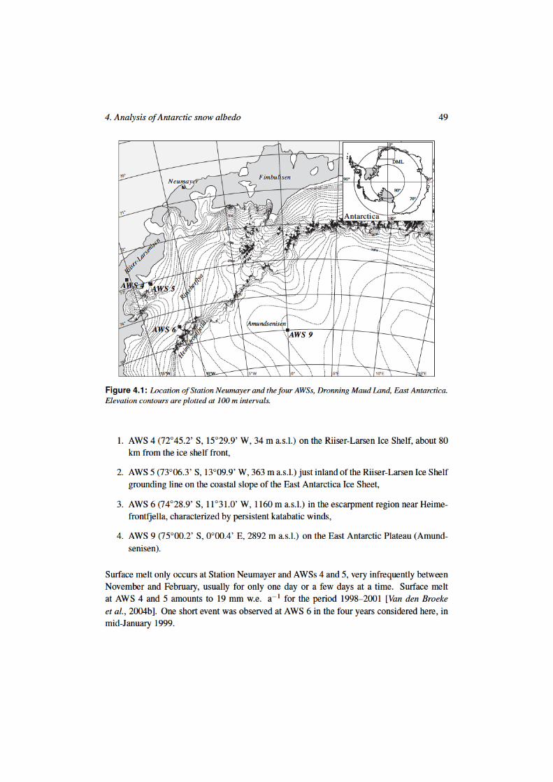
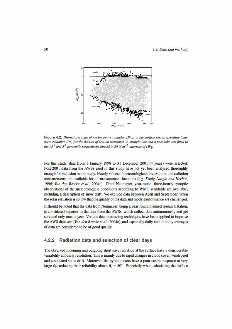
4. Analysis of Antarctic snow albedo 51
albedo using individual pairs of hourly SW, (reflected shortwave radiation) and SW+ (globalshortwave radiation), the errors in the albedo values become rather large at higher #0. Wetherefore resorted to daily averages, whereby the albedo averaged over 24 h is calculatedusing the daily accumulated SW -fluxes.
Daily averages of cloud cover N+ are estimated using the longwave (LW ) fluxes, for consis-tency also at Neumayer where synoptic observations are being carried out. Despite extremecare, synoptic observations do suffer from some subjectiveness. Moreover, synoptically ob-tained cloud cover may not always reflect the governing radiation balance, e.g. when the skyis fully covered with very thin clouds through which the sun disk is still visible, or when athin layer of fog is present close to the surface.
We calculated 24 h-averaged cloud cover by plotting LWnet (= LW,+ LW+) against LW, (seefigure 4.2). Positive fluxes are defined towards the surface. We fit a parabola and a straightline to the 5th and 95th percentile of daily averaged LW, [see also Van den Broeke et al.,2004c, 2006]. The highest percentile corresponds to the most cloudy days (N+ = 1), as thesnow surface is in thermal equilibrium with the warm cloud base under cloudy conditions —then LWnet is approximately zero. The lowest percentile of the data points correspond to thedays with clearest sky (N+ = 0). A linear interpolation between the two fitted lines gives anestimate of the fractional cloud cover for all data points. From the total data set, a clear-sky(N+ < 0.2) subset is distilled, which are from now on referred to as clear days, or as clear-skyconditions. The choice for N+ = 0.2 is arbitrary from a physical point of view, but necessaryfor a data set of sufficient size.
4.2.3 Water vapour column sensitivity
Before the model is applied to field data, the sensitivity of modelled albedo to the atmo-spheric composition — and most notably the water vapour column — must be investigated.Throughout the year, water vapour is the most strongly varying absorbing gas in the (polar)atmosphere. Measurements on Antarctica [e.g. Van den Broeke et al., 2004a] reveal a factor 5to 10 difference between summer and winter surface specific humidity. This is primarily dueto the strong dependence of water vapour concentration on temperature through the Clausius-Clapeyron relation. As water vapour absorption bands are concentrated in the near-IR, thebroadband (spectrally integrated) albedo at the ground may increase when the water vapourcolumn is thicker. The magnitude of this effect is modelled using DAK, and demonstratedin figure 4.3 as the two solid lines, showing two model runs with a standard subarctic sum-mer and subarctic winter atmosphere [Anderson et al., 1986]. For all #0, the difference inbroadband albedo is about 0.013.
This effect can also be caused by differences in surface elevation. High on an ice sheetplateau, the atmosphere contains far less water vapour than in coastal regions or on iceshelves.
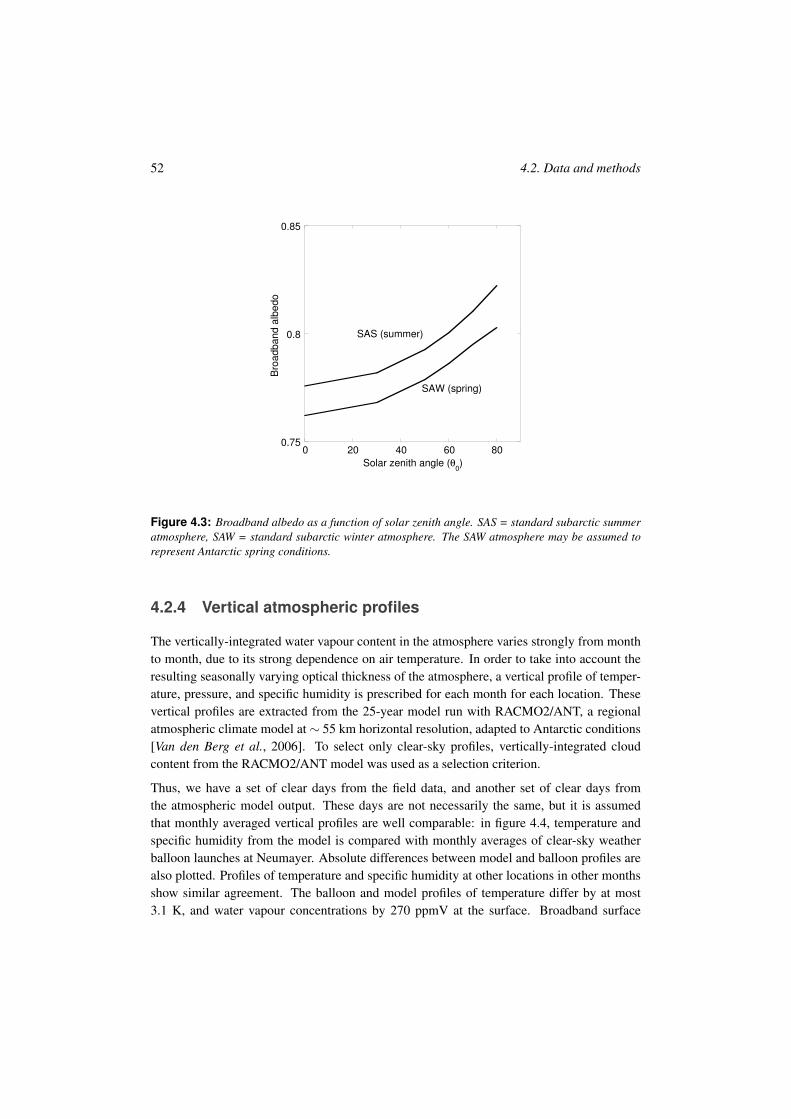
52 4.2. Data and methods
0.75
0.8
0.85
0 20 40 60 80
Bro
ad
ba
nd
alb
ed
o
Solar zenith angle (!0)
SAS (summer)
SAW (spring)
Figure 4.3: Broadband albedo as a function of solar zenith angle. SAS = standard subarctic summeratmosphere, SAW = standard subarctic winter atmosphere. The SAW atmosphere may be assumed torepresent Antarctic spring conditions.
4.2.4 Vertical atmospheric profiles
The vertically-integrated water vapour content in the atmosphere varies strongly from monthto month, due to its strong dependence on air temperature. In order to take into account theresulting seasonally varying optical thickness of the atmosphere, a vertical profile of temper-ature, pressure, and specific humidity is prescribed for each month for each location. Thesevertical profiles are extracted from the 25-year model run with RACMO2/ANT, a regionalatmospheric climate model at $ 55 km horizontal resolution, adapted to Antarctic conditions[Van den Berg et al., 2006]. To select only clear-sky profiles, vertically-integrated cloudcontent from the RACMO2/ANT model was used as a selection criterion.
Thus, we have a set of clear days from the field data, and another set of clear days fromthe atmospheric model output. These days are not necessarily the same, but it is assumedthat monthly averaged vertical profiles are well comparable: in figure 4.4, temperature andspecific humidity from the model is compared with monthly averages of clear-sky weatherballoon launches at Neumayer. Absolute differences between model and balloon profiles arealso plotted. Profiles of temperature and specific humidity at other locations in other monthsshow similar agreement. The balloon and model profiles of temperature differ by at most3.1 K, and water vapour concentrations by 270 ppmV at the surface. Broadband surface
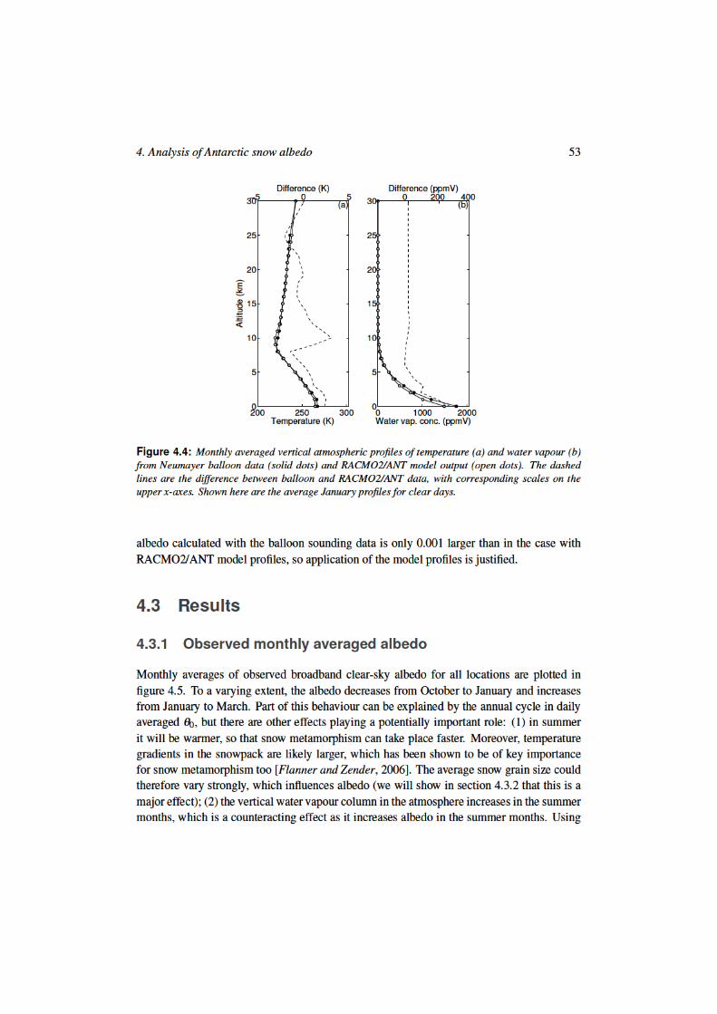
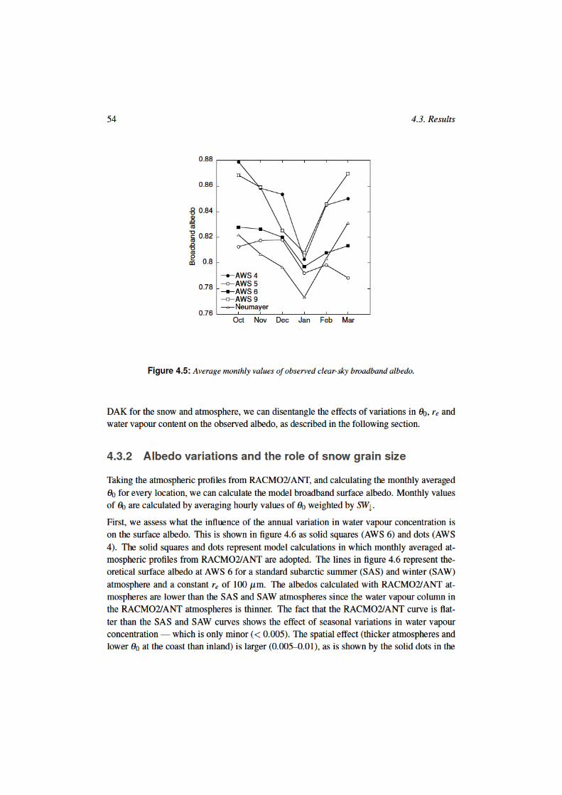
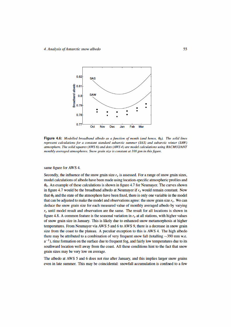
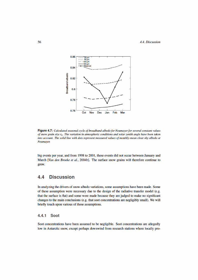
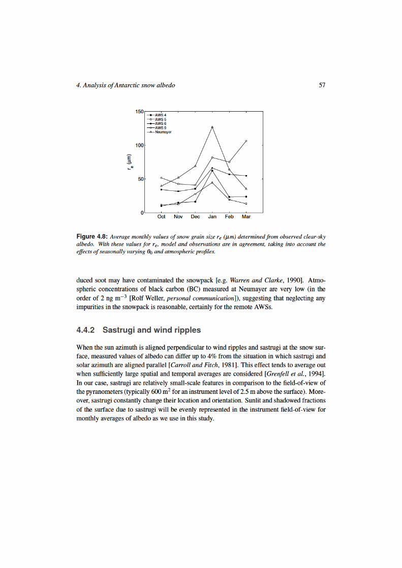
58 4.5. Summary and conclusions
4.4.3 Inclination of the snow surface
A small inclination of the surface can have a large impact on measured albedo, especially atlarge #0. In the case of daily or monthly averages, only the tilt component in the North-Southdirection is affected (see Grenfell et al. [1994] for example calculations). Large-scale tilt at allstations happens to be approximately in the North-South direction, varying from very small(< 0.1# at Neumayer, AWS 4 and 9) to 1.5# at AWS 6. However, these are values derivedfrom large-scale digital elevation maps, and only true on scales of several kilometers. Actualvalues for the surface in the sensor field-of-view are in fact unknown, but likely smaller than1# in any direction, because any larger slope would be clearly detectable in the field. As aworst-case scenario calculation, we suppose a slope of 1# and #0 = 80#. The daily meanalbedo is then off by 1.8% and errors in the inferred values of re would, in this case, beroughly 40%. This error decreases rapidly for lower #0 and flatter surfaces. For a slope of0.1# and #0 = 80#, the error in albedo decreases to 0.2% and the error in re would be 4%.
4.4.4 In-situ validation of snow grain size
Although the seasonal variation in snow grain size that we found is realistic and plausible,it turns out to be very difficult to independently verify whether this annual variation in snowgrain size is realistic – information about re at the measurement locations is non-existent.Recent accounts of snow grain sizes in the area are found in Gay et al. [2002] and Karkaset al. [2002], but are not readily convertible to an optically equivalent snow grain size due todifferent measurement techniques or different definitions of snow grain size.
Recent work from Scambos et al. [2007], using radiances from the MODIS satellite sensorsto retrieve snow grain size, suggests that summer-averaged (December–February) grain sizesrange from 76 µm at AWS 9 to 213 µm at Neumayer. A comparison between our results andthe MODIS-derived snow grain sizes (both averages for the Dec – Feb period) is shown in fig-ure 4.9. Although there is a good correlation between the two, the MODIS-derived re is morethan twice as large. The MODIS product calculates one value for re from images obtainedthroughout the summer — it therefore implicitly assumes that re is constant throughout theyear. It could therefore be that Scambos et al. [2007] obtain larger snow grains when thereis a bias towards January scenes; or that in the months in which the MODIS product was ac-quired (Dec 2003 – Feb 2004), snow grains were on average larger. More research is requiredto explain the discrepancy.
4.5 Summary and conclusions
In this chapter, we have used a radiative transfer model DAK for calculating the albedo ofsnow surfaces. The radiative transfer model has been applied to a 4-year data set of solar

60 4.5. Summary and conclusions
Soot and dust concentrations can be prescribed. Practical applications will include East andWest Antarctica, the dry-snow zone of Greenland, and spring snow cover on other ice capsand tundras, but exclude surfaces with melt, heavy undulations, patchy snow, or ice surfaces.
With a growing contribution of remote sensing to the study of solar radiation in the snow-atmosphere system, it is of great importance to apply a uniform method of ground-truthingof snow properties. In the absence of this, we have shown that estimates of, and trends in,snow grain size can be obtained by combining model calculations with field measurementsof radiative fluxes. A next step would therefore be to apply DAK to a data set where allparameters relevant to albedo variations, including direct measurements on snow grain sizes,are measured simultaneously. In this way, a ‘closure’ of the model can be achieved.
5Cloud properties from radiation
measurements over snow and ice
Summary
We critically review and improve a simple method to extract year-round records of cloudoptical thickness from radiation measurements made by automatic weather stations (AWSs)over snow and ice surfaces. A ‘longwave-equivalent cloudiness’, N+ , obtained from long-wave radiation measurements, is combined with the effective cloud optical thickness, & , fromshortwave data, to obtain consistent, year-round information on cloud properties. The methodis applied to radiation data from six AWSs in Dronning Maud Land, Antarctica, and the abla-tion area of the West-Greenland ice sheet. The good correlation between daily-mean N+ and& for all locations (0.73 < r < 0.91) shows that shortwave radiative properties of clouds canbe inferred using longwave radiation even in the absence of solar radiation itself. An erroranalysis shows that retrievals of & are sensitive to the quality of the input data, but accuratewithin 7.5% for a 2% uncertainty in clear-sky incoming solar radiation. As three applicationsof the method, we discuss the influence of clouds on the radiation budget (Application I), therelation between cloud cover and broadband albedo (II) at the six AWS locations, and wedemonstrate the possibility to detect trends in & in longer data series (III). About 1/3 of theattenuation of solar radiation by clouds is compensated by multiple reflections between thehigh-albedo surface and the cloud base (Appl. I). Cloudy-sky surface albedo is higher thanthe clear-sky albedo for snow surfaces but not for ice (Appl. II): over snow surfaces, cloudsdeplete near-infrared radiation and thus increase the broadband albedo. Ice surfaces, have amuch lower albedo for visible radiation, weakening this enrichment of visible radiation andthus the increase of broadband albedo. The method is used to detect a trend of decreasing &in the long time series from Neumayer in the period 1995–2004 (Appl. III).
This chapter is based on Kuipers Munneke, P., C. H. Reijmer and M. R. van den Broeke (2009), Assessing theretrieval of cloud properties from radiation measurements over snow and ice. Submitted to Int. J. Climatol.
61
62 5.1. Introduction
5.1 Introduction
The influence of Earth’s climate on glaciers and ice sheets is enforced through the surfaceenergy budget (SEB), whose dominant terms are the longwave and shortwave radiative fluxes.The SEB strongly influences the summer surface mass balance of glaciers and ice sheets intheir ablation areas, as it largely determines the rate and amount of melt. If meltwater runoffexceeds mass gain by precipitation, sea level will rise. Small glaciers have been contributingto sea-level rise in this way already since the Little Ice Age [e.g. Dyurgerov and Meier,2005]. Recent studies indicate that the Greenland ice sheet is also contributing to sea-levelrise [Shepherd and Wingham, 2007], both by means of a decreasing surface mass balance[Box et al., 2006] and through ice-dynamical effects that are possibly triggered by meltwaterinput [Rignot et al., 2008]. Knowledge of the SEB of glaciers and ice sheets is thereforeimportant.
The SEB is greatly altered in the presence of clouds. The longwave radiation emitted to thesurface will increase, since the emissivity of clouds is higher than that of a clear sky. Theshortwave radiation field is rather complex in the presence of clouds, especially over highlyreflective surfaces such as snow and ice. First of all, clouds reduce the incoming radiationflux by reflection and absorption. Secondly, the radiation that passes through the cloud willbe subject to multiple reflections between the surface and the cloud base [Angstrom and Try-selius, 1934; Schneider and Dickinson, 1976; Shine, 1984]. Since the spectral albedo of snow(and ice) and the absorption of radiation by clouds are both strongly dependent on wavelength[Liljequist, 1956; Wiscombe and Warren, 1980], the magnitude of cloud effects is also verymuch wavelength-dependent — clouds not only alter the intensity, but also the spectral com-position of the solar radiation arriving at the surface. At the same time, spectrally-integrated(broadband) albedo has been observed to increase in the presence of clouds [Liljequist, 1956;Ambach, 1974]. All these phenomena have competing effects on the shortwave radiationbudget of the snow surface.
An outstanding problem in the study of clouds is the lack of cloud observations over icesheets. From satellite data, it is difficult to infer properties of clouds because clouds andsnow appear very similar both in the solar spectrum as in their thermal properties [e.g. Townet al., 2007]. This hampers the study of clouds over ice sheets. The increasing amount ofAutomatic Weather Stations (AWS) on glaciers and ice sheets [Stearns and Wendler, 1988;Allison et al., 1993; Van den Broeke et al., 2004a, 2008a] are a possibly valuable source ofinformation from remote locations, that could make more data on cloud properties available.
The attempt to obtain cloud properties in polar regions using ground-based measurementsis not new. Mahesh et al. [2001] use a Fourier transform interferometer to determine cloudoptical thickness at South Pole station. Long and Ackerman [2000] present a method toestimate cloud fraction (N) using global and diffuse solar radiation measurements, whichlimits the application to daytime periods, and to locations where diffuse shortwave radiationis measured. Marty and Philipona [2000] present the Clear-Sky Index to separate clear and
5. Cloud properties over snow and ice 63
cloudy skies using longwave radiation measurements, the derivation of which is to a largeextent based on Konzelmann et al. [1994]. Durr and Philipona [2004] extend the Clear-Sky Index to an algorithm that retrieves N from downwelling longwave measurements. Acaveat of the traditional cloud fraction N, be it observed by a meteorologist or retrieved usingan algorithm, is that it does not necessarily provide an accurate description of the radiativeproperties of the cloud cover.
In the method central in this chapter, a ‘longwave-equivalent’ cloudiness N+ is determinedfrom the apparent emissivity of the sky and surface temperature. Similarly, shortwave radia-tion measurements can be used to obtain the cloud optical thickness, & [Stephens, 1984], fol-lowing a parameterization developed by Fitzpatrick et al. [2004]. Cloud optical thickness isdefined in terms of cloud microphysical parameters and represents a measure for the amountof radiation that is attenuated by the cloud. Combining the parameterization by Fitzpatricket al. [2004] and the retrieval of N+ , a simple method is obtained that makes use of radiationmeasurements from AWSs over snow and ice surfaces to gain knowledge about year-roundradiative cloud properties. This method was first used by Van den Broeke et al. [2008a] todetermine cloud optical properties over Greenland stations, and by Giesen et al. [2009] forMidtdalsbreen and Storbreen, two glaciers in southern Norway.
In this chapter, we will review the method, present some improvements, and subject themethod to a critical review of potential uncertainties. As a final part, we demonstrate theversatility of the method in three different applications (section 5.4). The method can beuseful (a) to those that wish to extend the amount of information that can be gained fromtheir AWSs, and (b) to those that are looking for validation data of satellite retrievals of cloudoptical thickness.
5.2 Data and methods
5.2.1 Description of data
We use data from six locations, five of which are continuously recording AWSs — three inGreenland and two in Antarctica — and the sixth is the manned BSRN (Baseline SurfaceRadiation Network, [Ohmura et al., 1998]) station Neumayer in Antarctica (figure 5.1). Ashort characterization of each of these locations and corresponding data sets is given in Table5.1. The AWSs, which are part of a larger network of sites [Van den Broeke et al., 2004a,2008a], were selected for their continuous data sets of radiation, without data gaps caused bye.g. sensor riming, frost accretion, snow accumulation, or instrument malfunction. The threeAntarctic locations Neumayer, AWS 5 and AWS 6 (figure 5.1(a)) are located in DronningMaud Land (East Antarctica) on the ice shelf, the coastal ice sheet and the escarpment region,respectively [Van den Broeke et al., 2004a]. The three Greenlandic stations (figure 5.1(b)) arepart of the Kangerlussuaq transect (K-transect), located at the western edge of the Greenland

64 5.2. Data and methods
Table5.1:
Specificationsfor
thedata
setsused
inthis
study.
Antarctica
Greenland
Neum
ayerAW
S5
AWS
6S5
S6S9
Latitude70 #37’S
73 #06’S74 #29’S
67 #06’N67 #05’N
67 #03’NLongitude
8 #22’W13 #10’W
11 #31’W50 #07’W
49 #23’W48 #14’W
Altitude
(ma.s.l.)
42363
1160490
10201520
Iceedge
dist.(km)
5105
2806
3888
Temperature
( #C)
"15.9
a"
16.4b
"16.6
b"
5.5c
"9.8
c"
12.6c
Pyranometer
K&
Zd
CM
11K
&Z
CM
3K
&Z
CM
3K
&Z
CM
3K
&Z
CM
3K
&Z
CM
3Pyrgeom
eterEppley
PIRK
&Z
CG
3K
&Z
CG
3K
&Z
CG
3K
&Z
CG
3K
&Z
CG
3Sam
pl.period(m
in)1/60
66
66
6A
verag.period(m
in)1
120120
6060
60Startdate
ofset1
Jan1995
1Jan
19981
Jan1998
28A
ug2003
1Sep
20031
Sep2003
Enddate
ofset31
Dec
200431
Dec
200131
Dec
200127
Aug
200731
Aug
200731
Aug
2007
aAnnualavg
at2m
levelbA
nnualavgatinstr
level(approx2
m)
cAnnualavg
atinstrlevel(approx
6m
)dK
&Z
=K
ipp&
Zonen
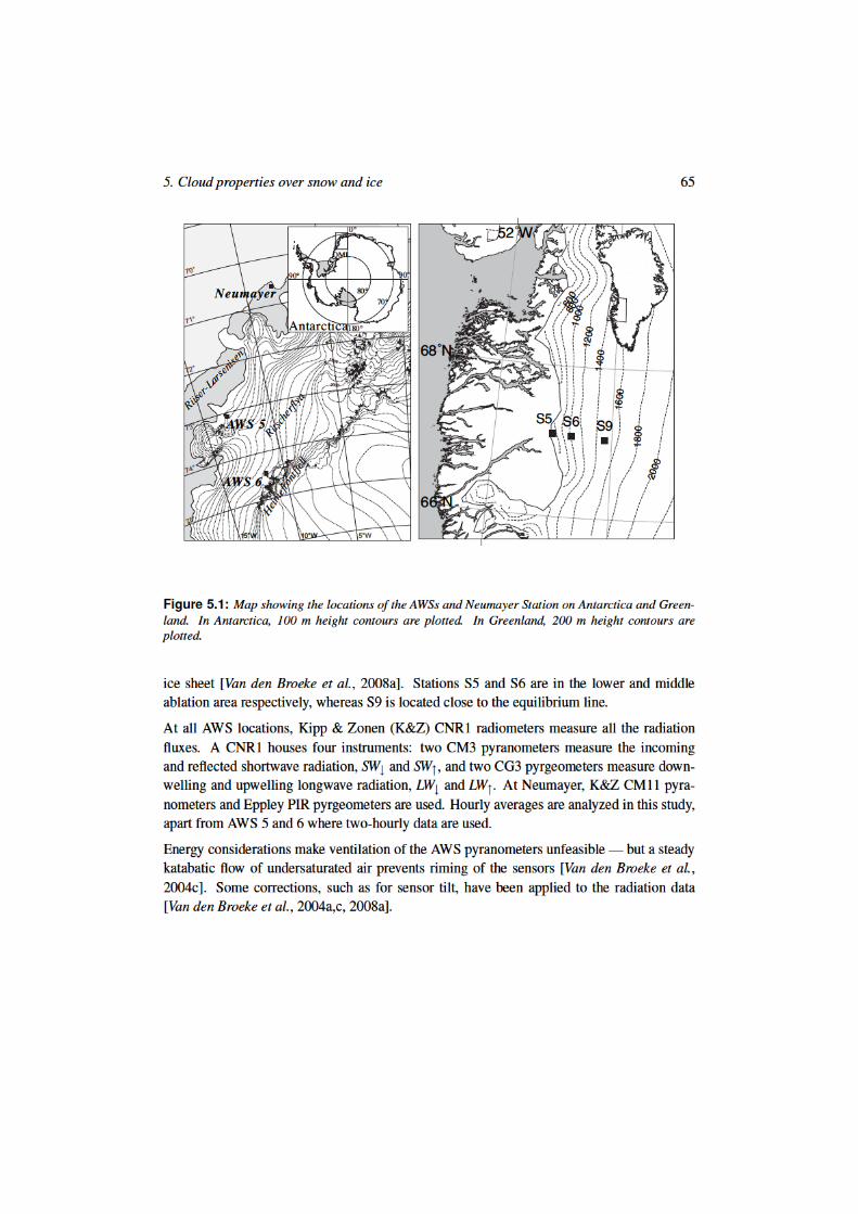
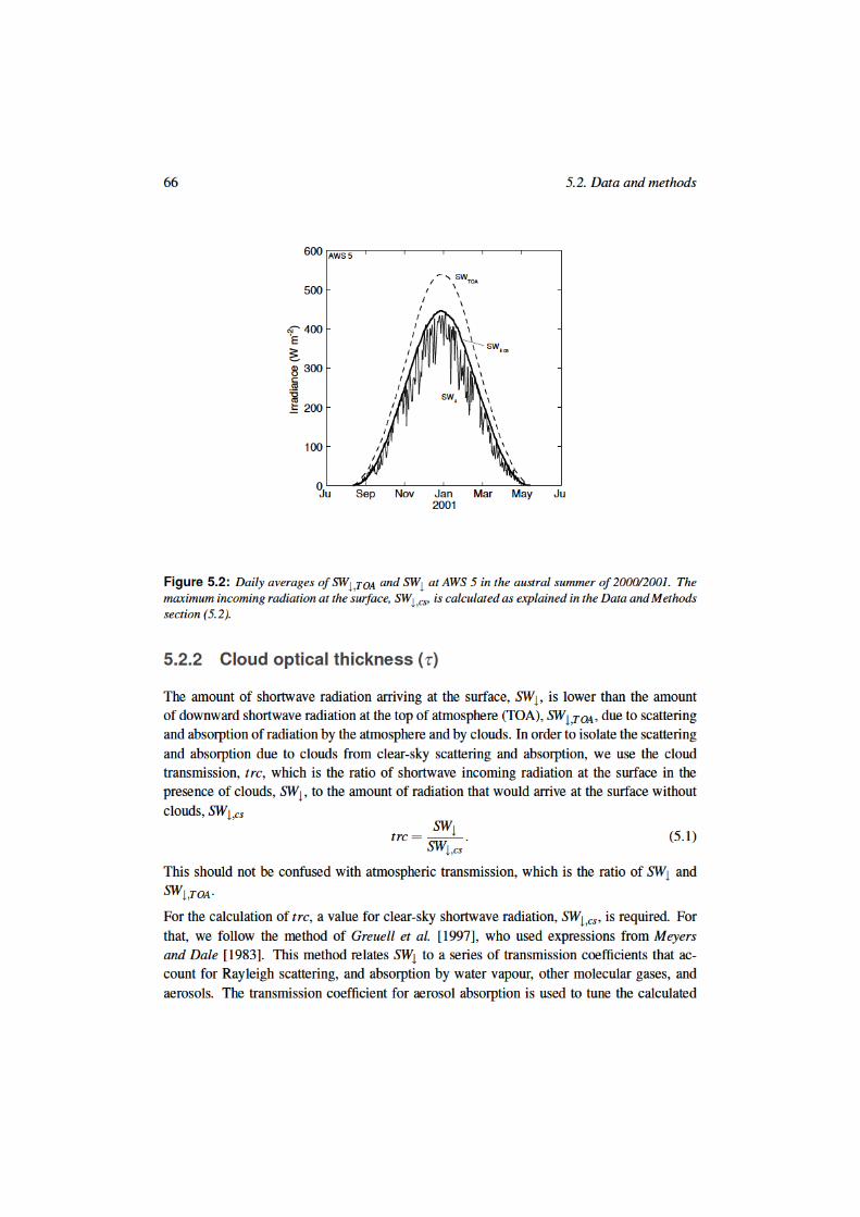
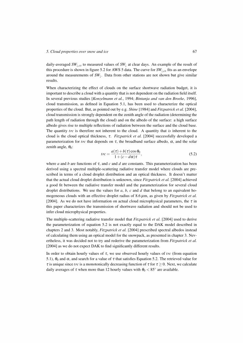
5. Cloud properties over snow and ice 67
daily-averaged SW+,cs to measured values of SW+ at clear days. An example of the result ofthis procedure is shown in figure 5.2 for AWS 5 data. The curve for SW+,cs fits as an envelopearound the measurements of SW+. Data from other stations are not shown but give similarresults.
When characterizing the effect of clouds on the surface shortwave radiation budget, it isimportant to describe a cloud with a quantity that is not dependent on the radiation field itself.In several previous studies [Konzelmann et al., 1994; Bintanja and van den Broeke, 1996],cloud transmission, as defined in Equation 5.1, has been used to characterize the opticalproperties of the cloud. But, as pointed out by e.g. Shine [1984] and Fitzpatrick et al. [2004],cloud transmission is strongly dependent on the zenith angle of the radiation (determining thepath length of radiation through the cloud) and on the albedo of the surface: a high surfacealbedo gives rise to multiple reflections of radiation between the surface and the cloud base.The quantity trc is therefore not inherent to the cloud. A quantity that is inherent to thecloud is the cloud optical thickness, & . Fitzpatrick et al. [2004] successfully developed aparameterization for trc that depends on & , the broadband surface albedo, ! , and the solarzenith angle, #0:
trc =a(&)+b(&)cos#0
1+(c"d!)&, (5.2)
where a and b are functions of & , and c and d are constants. This parameterization has beenderived using a spectral multiple-scattering radiative transfer model where clouds are pre-scribed in terms of a cloud droplet distribution and an optical thickness. It doesn’t matterthat the actual cloud droplet distribution is unknown, since Fitzpatrick et al. [2004] achieveda good fit between the radiative transfer model and the parameterization for several clouddroplet distributions. We use the values for a, b, c and d that belong to an equivalent ho-mogeneous clouds with an effective droplet radius of 8.6 µm, as given by Fitzpatrick et al.[2004]. As we do not have information on actual cloud microphysical parameters, the & inthis paper characterizes the transmission of shortwave radiation and should not be used toinfer cloud microphysical properties.
The multiple-scattering radiative transfer model that Fitzpatrick et al. [2004] used to derivethe parameterization of equation 5.2 is not exactly equal to the DAK model described inchapters 2 and 3. Most notably, Fitzpatrick et al. [2004] prescribed spectral albedos insteadof calculating them using an optical model for the snowpack, as presented in chapter 3. Nev-ertheless, it was decided not to try and rederive the parameterization from Fitzpatrick et al.[2004] as we do not expect DAK to find significantly different results.
In order to obtain hourly values of & , we use observed hourly values of trc (from equation5.1), #0 and ! , and search for a value of & that satisfies Equation 5.2. The retrieved value for& is unique since trc is a monotonically decreasing function of & for & . 0. Next, we calculatedaily averages of & when more than 12 hourly values with #0 < 85# are available.
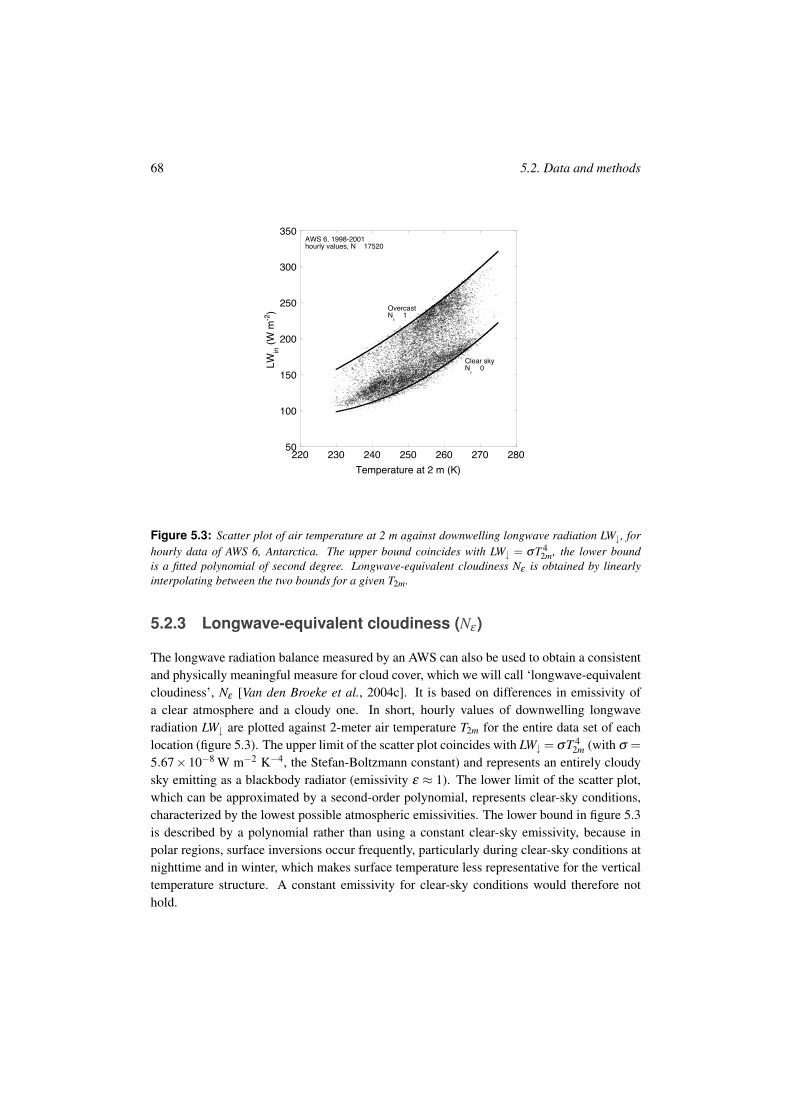
68 5.2. Data and methods
50
100
150
200
250
300
350
220 230 240 250 260 270 280
LW
in (
W m
-2)
Temperature at 2 m (K)
AWS 6, 1998-2001hourly values, N 17520
Clear skyN! 0
OvercastN! 1
Figure 5.3: Scatter plot of air temperature at 2 m against downwelling longwave radiation LW+, forhourly data of AWS 6, Antarctica. The upper bound coincides with LW+ = %T 4
2m, the lower boundis a fitted polynomial of second degree. Longwave-equivalent cloudiness N+ is obtained by linearlyinterpolating between the two bounds for a given T2m.
5.2.3 Longwave-equivalent cloudiness (N+ )
The longwave radiation balance measured by an AWS can also be used to obtain a consistentand physically meaningful measure for cloud cover, which we will call ‘longwave-equivalentcloudiness’, N+ [Van den Broeke et al., 2004c]. It is based on differences in emissivity ofa clear atmosphere and a cloudy one. In short, hourly values of downwelling longwaveradiation LW+ are plotted against 2-meter air temperature T2m for the entire data set of eachlocation (figure 5.3). The upper limit of the scatter plot coincides with LW+ = %T 4
2m (with % =5.67% 10"8 W m"2 K"4, the Stefan-Boltzmann constant) and represents an entirely cloudysky emitting as a blackbody radiator (emissivity + / 1). The lower limit of the scatter plot,which can be approximated by a second-order polynomial, represents clear-sky conditions,characterized by the lowest possible atmospheric emissivities. The lower bound in figure 5.3is described by a polynomial rather than using a constant clear-sky emissivity, because inpolar regions, surface inversions occur frequently, particularly during clear-sky conditions atnighttime and in winter, which makes surface temperature less representative for the verticaltemperature structure. A constant emissivity for clear-sky conditions would therefore nothold.
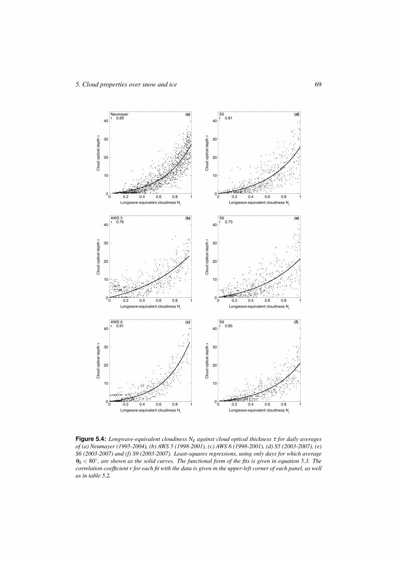
5. Cloud properties over snow and ice 69
0
10
20
30
40
0 0.2 0.4 0.6 0.8 1
Clo
ud
op
tica
l d
ep
th !
Longwave-equivalent cloudiness N"
Neumayerr 0.89
(a)
0
10
20
30
40
0 0.2 0.4 0.6 0.8 1
Clo
ud
op
tica
l d
ep
th !
Longwave-equivalent cloudiness N"
S5r 0.81
(d)
0
10
20
30
40
0 0.2 0.4 0.6 0.8 1
Clo
ud
op
tica
l d
ep
th !
Longwave-equivalent cloudiness N"
AWS 5r 0.76
(b)
0
10
20
30
40
0 0.2 0.4 0.6 0.8 1
Clo
ud
op
tica
l d
ep
th !
Longwave-equivalent cloudiness N"
S6r 0.73
(e)
0
10
20
30
40
0 0.2 0.4 0.6 0.8 1
Clo
ud
op
tica
l d
ep
th !
Longwave-equivalent cloudiness N"
AWS 6r 0.91
(c)
0
10
20
30
40
0 0.2 0.4 0.6 0.8 1
Clo
ud
op
tica
l d
ep
th !
Longwave-equivalent cloudiness N"
S9r 0.85
(f)
Figure 5.4: Longwave-equivalent cloudiness N+ against cloud optical thickness & for daily averagesof (a) Neumayer (1995-2004), (b) AWS 5 (1998-2001), (c) AWS 6 (1998-2001), (d) S5 (2003-2007), (e)S6 (2003-2007) and (f) S9 (2003-2007). Least-squares regressions, using only days for which average#0 < 80#, are shown as the solid curves. The functional form of the fits is given in equation 5.3. Thecorrelation coefficient r for each fit with the data is given in the upper-left corner of each panel, as wellas in table 5.2.
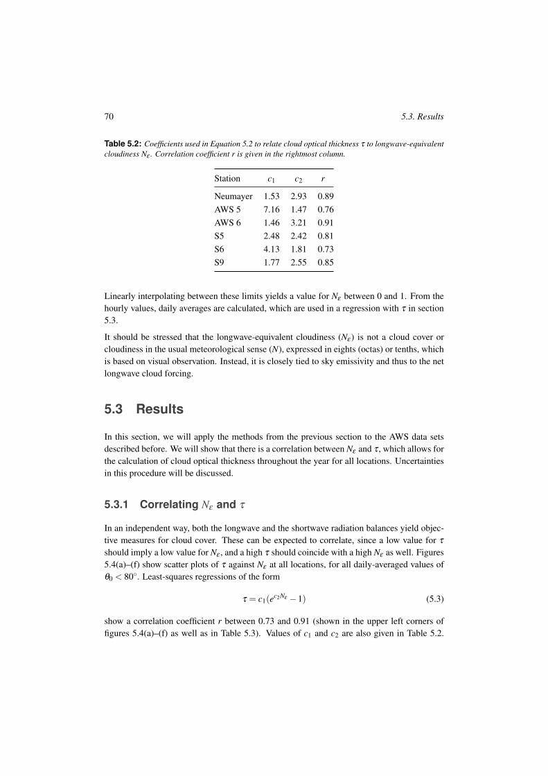
70 5.3. Results
Table 5.2: Coefficients used in Equation 5.2 to relate cloud optical thickness & to longwave-equivalentcloudiness N+ . Correlation coefficient r is given in the rightmost column.
Station c1 c2 r
Neumayer 1.53 2.93 0.89AWS 5 7.16 1.47 0.76AWS 6 1.46 3.21 0.91S5 2.48 2.42 0.81S6 4.13 1.81 0.73S9 1.77 2.55 0.85
Linearly interpolating between these limits yields a value for N+ between 0 and 1. From thehourly values, daily averages are calculated, which are used in a regression with & in section5.3.
It should be stressed that the longwave-equivalent cloudiness (N+ ) is not a cloud cover orcloudiness in the usual meteorological sense (N), expressed in eights (octas) or tenths, whichis based on visual observation. Instead, it is closely tied to sky emissivity and thus to the netlongwave cloud forcing.
5.3 Results
In this section, we will apply the methods from the previous section to the AWS data setsdescribed before. We will show that there is a correlation between N+ and & , which allows forthe calculation of cloud optical thickness throughout the year for all locations. Uncertaintiesin this procedure will be discussed.
5.3.1 Correlating N+ and &
In an independent way, both the longwave and the shortwave radiation balances yield objec-tive measures for cloud cover. These can be expected to correlate, since a low value for &should imply a low value for N+ , and a high & should coincide with a high N+ as well. Figures5.4(a)–(f) show scatter plots of & against N+ at all locations, for all daily-averaged values of#0 < 80#. Least-squares regressions of the form
& = c1(ec2N+ "1) (5.3)
show a correlation coefficient r between 0.73 and 0.91 (shown in the upper left corners offigures 5.4(a)–(f) as well as in Table 5.3). Values of c1 and c2 are also given in Table 5.2.
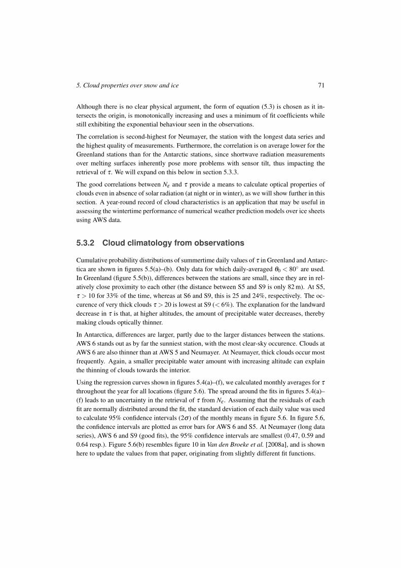
5. Cloud properties over snow and ice 71
Although there is no clear physical argument, the form of equation (5.3) is chosen as it in-tersects the origin, is monotonically increasing and uses a minimum of fit coefficients whilestill exhibiting the exponential behaviour seen in the observations.
The correlation is second-highest for Neumayer, the station with the longest data series andthe highest quality of measurements. Furthermore, the correlation is on average lower for theGreenland stations than for the Antarctic stations, since shortwave radiation measurementsover melting surfaces inherently pose more problems with sensor tilt, thus impacting theretrieval of & . We will expand on this below in section 5.3.3.
The good correlations between N+ and & provide a means to calculate optical properties ofclouds even in absence of solar radiation (at night or in winter), as we will show further in thissection. A year-round record of cloud characteristics is an application that may be useful inassessing the wintertime performance of numerical weather prediction models over ice sheetsusing AWS data.
5.3.2 Cloud climatology from observations
Cumulative probability distributions of summertime daily values of & in Greenland and Antarc-tica are shown in figures 5.5(a)–(b). Only data for which daily-averaged #0 < 80# are used.In Greenland (figure 5.5(b)), differences between the stations are small, since they are in rel-atively close proximity to each other (the distance between S5 and S9 is only 82 m). At S5,& > 10 for 33% of the time, whereas at S6 and S9, this is 25 and 24%, respectively. The oc-curence of very thick clouds & > 20 is lowest at S9 (< 6%). The explanation for the landwarddecrease in & is that, at higher altitudes, the amount of precipitable water decreases, therebymaking clouds optically thinner.
In Antarctica, differences are larger, partly due to the larger distances between the stations.AWS 6 stands out as by far the sunniest station, with the most clear-sky occurence. Clouds atAWS 6 are also thinner than at AWS 5 and Neumayer. At Neumayer, thick clouds occur mostfrequently. Again, a smaller precipitable water amount with increasing altitude can explainthe thinning of clouds towards the interior.
Using the regression curves shown in figures 5.4(a)–(f), we calculated monthly averages for &throughout the year for all locations (figure 5.6). The spread around the fits in figures 5.4(a)–(f) leads to an uncertainty in the retrieval of & from N+ . Assuming that the residuals of eachfit are normally distributed around the fit, the standard deviation of each daily value was usedto calculate 95% confidence intervals (2% ) of the monthly means in figure 5.6. In figure 5.6,the confidence intervals are plotted as error bars for AWS 6 and S5. At Neumayer (long dataseries), AWS 6 and S9 (good fits), the 95% confidence intervals are smallest (0.47, 0.59 and0.64 resp.). Figure 5.6(b) resembles figure 10 in Van den Broeke et al. [2008a], and is shownhere to update the values from that paper, originating from slightly different fit functions.
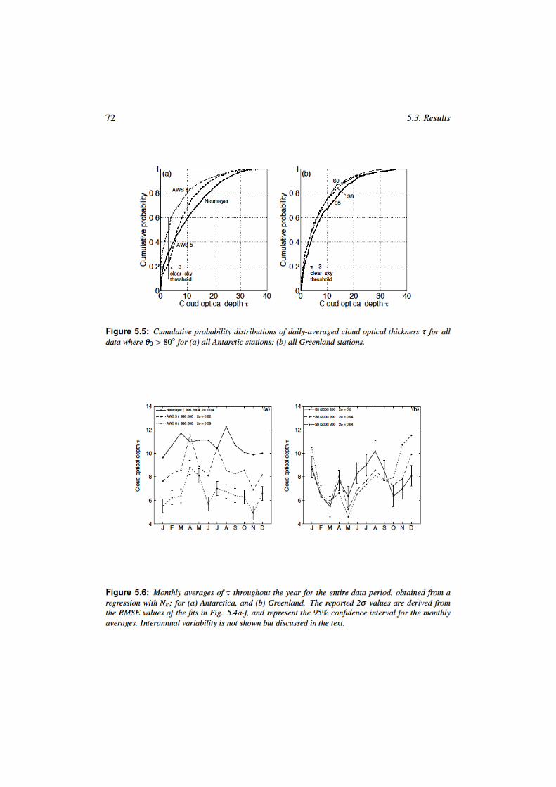
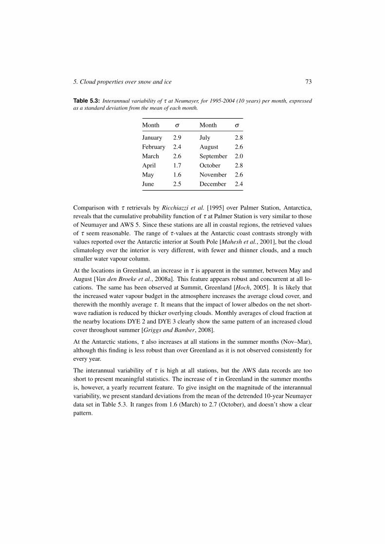
5. Cloud properties over snow and ice 73
Table 5.3: Interannual variability of & at Neumayer, for 1995-2004 (10 years) per month, expressedas a standard deviation from the mean of each month.
Month % Month %
January 2.9 July 2.8February 2.4 August 2.6March 2.6 September 2.0April 1.7 October 2.8May 1.6 November 2.6June 2.5 December 2.4
Comparison with & retrievals by Ricchiazzi et al. [1995] over Palmer Station, Antarctica,reveals that the cumulative probability function of & at Palmer Station is very similar to thoseof Neumayer and AWS 5. Since these stations are all in coastal regions, the retrieved valuesof & seem reasonable. The range of &-values at the Antarctic coast contrasts strongly withvalues reported over the Antarctic interior at South Pole [Mahesh et al., 2001], but the cloudclimatology over the interior is very different, with fewer and thinner clouds, and a muchsmaller water vapour column.
At the locations in Greenland, an increase in & is apparent in the summer, between May andAugust [Van den Broeke et al., 2008a]. This feature appears robust and concurrent at all lo-cations. The same has been observed at Summit, Greenland [Hoch, 2005]. It is likely thatthe increased water vapour budget in the atmosphere increases the average cloud cover, andtherewith the monthly average & . It means that the impact of lower albedos on the net short-wave radiation is reduced by thicker overlying clouds. Monthly averages of cloud fraction atthe nearby locations DYE 2 and DYE 3 clearly show the same pattern of an increased cloudcover throughout summer [Griggs and Bamber, 2008].
At the Antarctic stations, & also increases at all stations in the summer months (Nov–Mar),although this finding is less robust than over Greenland as it is not observed consistently forevery year.
The interannual variability of & is high at all stations, but the AWS data records are tooshort to present meaningful statistics. The increase of & in Greenland in the summer monthsis, however, a yearly recurrent feature. To give insight on the magnitude of the interannualvariability, we present standard deviations from the mean of the detrended 10-year Neumayerdata set in Table 5.3. It ranges from 1.6 (March) to 2.7 (October), and doesn’t show a clearpattern.
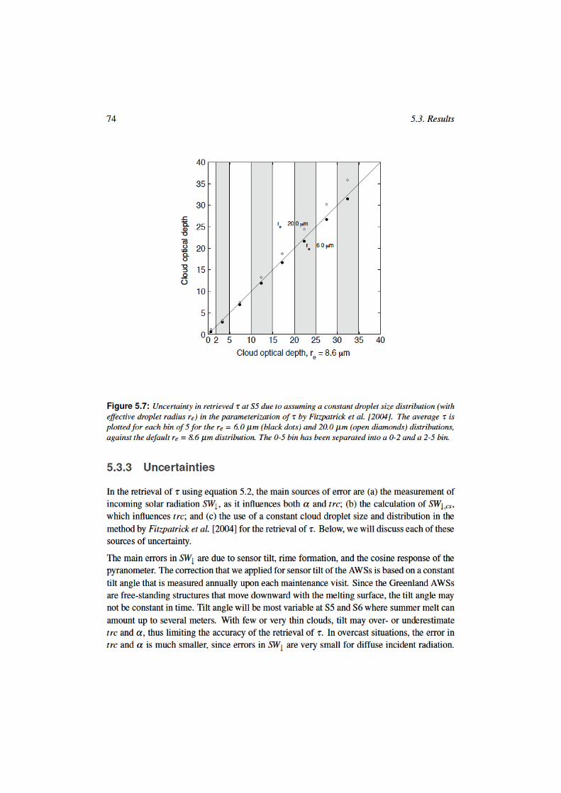
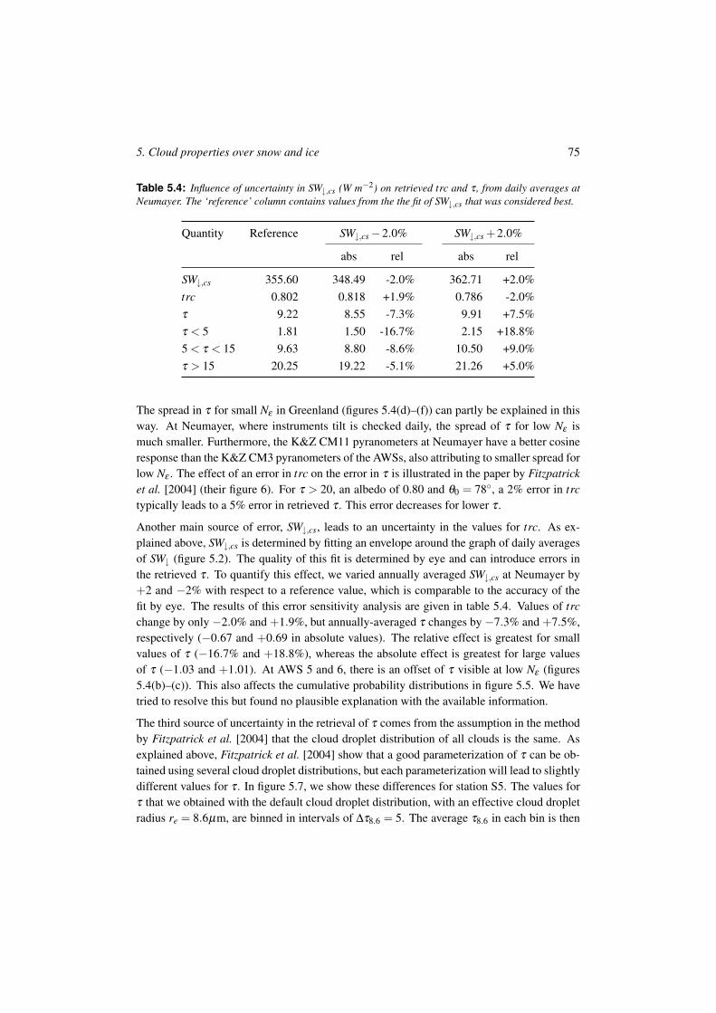
5. Cloud properties over snow and ice 75
Table 5.4: Influence of uncertainty in SW+,cs (W m"2) on retrieved trc and & , from daily averages atNeumayer. The ‘reference’ column contains values from the the fit of SW+,cs that was considered best.
Quantity Reference SW+,cs"2.0% SW+,cs +2.0%
abs rel abs rel
SW+,cs 355.60 348.49 -2.0% 362.71 +2.0%trc 0.802 0.818 +1.9% 0.786 -2.0%& 9.22 8.55 -7.3% 9.91 +7.5%& < 5 1.81 1.50 -16.7% 2.15 +18.8%5 < & < 15 9.63 8.80 -8.6% 10.50 +9.0%& > 15 20.25 19.22 -5.1% 21.26 +5.0%
The spread in & for small N+ in Greenland (figures 5.4(d)–(f)) can partly be explained in thisway. At Neumayer, where instruments tilt is checked daily, the spread of & for low N+ ismuch smaller. Furthermore, the K&Z CM11 pyranometers at Neumayer have a better cosineresponse than the K&Z CM3 pyranometers of the AWSs, also attributing to smaller spread forlow N+ . The effect of an error in trc on the error in & is illustrated in the paper by Fitzpatricket al. [2004] (their figure 6). For & > 20, an albedo of 0.80 and #0 = 78#, a 2% error in trctypically leads to a 5% error in retrieved & . This error decreases for lower & .
Another main source of error, SW+,cs, leads to an uncertainty in the values for trc. As ex-plained above, SW+,cs is determined by fitting an envelope around the graph of daily averagesof SW+ (figure 5.2). The quality of this fit is determined by eye and can introduce errors inthe retrieved & . To quantify this effect, we varied annually averaged SW+,cs at Neumayer by+2 and "2% with respect to a reference value, which is comparable to the accuracy of thefit by eye. The results of this error sensitivity analysis are given in table 5.4. Values of trcchange by only "2.0% and +1.9%, but annually-averaged & changes by "7.3% and +7.5%,respectively ("0.67 and +0.69 in absolute values). The relative effect is greatest for smallvalues of & ("16.7% and +18.8%), whereas the absolute effect is greatest for large valuesof & ("1.03 and +1.01). At AWS 5 and 6, there is an offset of & visible at low N+ (figures5.4(b)–(c)). This also affects the cumulative probability distributions in figure 5.5. We havetried to resolve this but found no plausible explanation with the available information.
The third source of uncertainty in the retrieval of & comes from the assumption in the methodby Fitzpatrick et al. [2004] that the cloud droplet distribution of all clouds is the same. Asexplained above, Fitzpatrick et al. [2004] show that a good parameterization of & can be ob-tained using several cloud droplet distributions, but each parameterization will lead to slightlydifferent values for & . In figure 5.7, we show these differences for station S5. The values for& that we obtained with the default cloud droplet distribution, with an effective cloud dropletradius re = 8.6µm, are binned in intervals of $&8.6 = 5. The average &8.6 in each bin is then
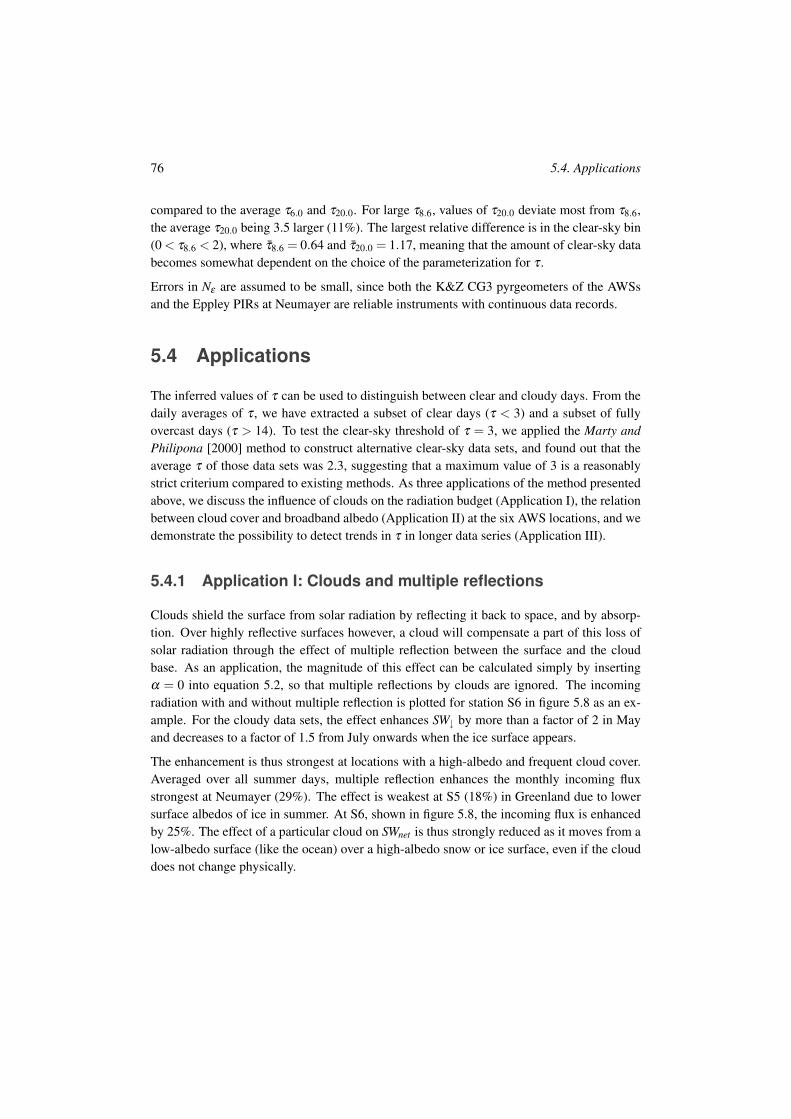
76 5.4. Applications
compared to the average &6.0 and &20.0. For large &8.6, values of &20.0 deviate most from &8.6,the average &20.0 being 3.5 larger (11%). The largest relative difference is in the clear-sky bin(0 < &8.6 < 2), where &8.6 = 0.64 and &20.0 = 1.17, meaning that the amount of clear-sky databecomes somewhat dependent on the choice of the parameterization for & .
Errors in N+ are assumed to be small, since both the K&Z CG3 pyrgeometers of the AWSsand the Eppley PIRs at Neumayer are reliable instruments with continuous data records.
5.4 Applications
The inferred values of & can be used to distinguish between clear and cloudy days. From thedaily averages of & , we have extracted a subset of clear days (& < 3) and a subset of fullyovercast days (& > 14). To test the clear-sky threshold of & = 3, we applied the Marty andPhilipona [2000] method to construct alternative clear-sky data sets, and found out that theaverage & of those data sets was 2.3, suggesting that a maximum value of 3 is a reasonablystrict criterium compared to existing methods. As three applications of the method presentedabove, we discuss the influence of clouds on the radiation budget (Application I), the relationbetween cloud cover and broadband albedo (Application II) at the six AWS locations, and wedemonstrate the possibility to detect trends in & in longer data series (Application III).
5.4.1 Application I: Clouds and multiple reflections
Clouds shield the surface from solar radiation by reflecting it back to space, and by absorp-tion. Over highly reflective surfaces however, a cloud will compensate a part of this loss ofsolar radiation through the effect of multiple reflection between the surface and the cloudbase. As an application, the magnitude of this effect can be calculated simply by inserting! = 0 into equation 5.2, so that multiple reflections by clouds are ignored. The incomingradiation with and without multiple reflection is plotted for station S6 in figure 5.8 as an ex-ample. For the cloudy data sets, the effect enhances SW+ by more than a factor of 2 in Mayand decreases to a factor of 1.5 from July onwards when the ice surface appears.
The enhancement is thus strongest at locations with a high-albedo and frequent cloud cover.Averaged over all summer days, multiple reflection enhances the monthly incoming fluxstrongest at Neumayer (29%). The effect is weakest at S5 (18%) in Greenland due to lowersurface albedos of ice in summer. At S6, shown in figure 5.8, the incoming flux is enhancedby 25%. The effect of a particular cloud on SWnet is thus strongly reduced as it moves from alow-albedo surface (like the ocean) over a high-albedo snow or ice surface, even if the clouddoes not change physically.
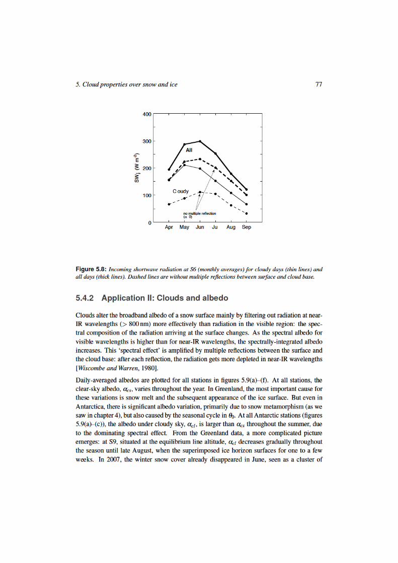
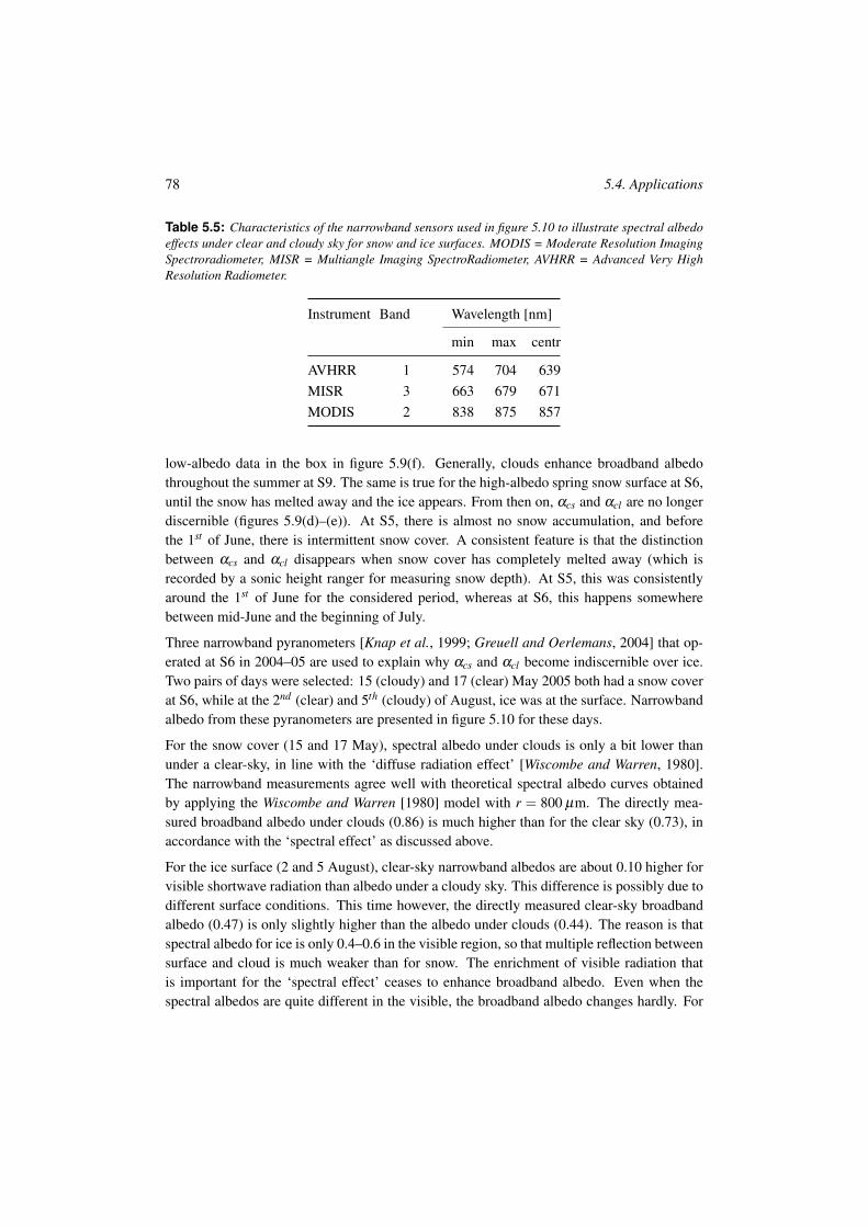
78 5.4. Applications
Table 5.5: Characteristics of the narrowband sensors used in figure 5.10 to illustrate spectral albedoeffects under clear and cloudy sky for snow and ice surfaces. MODIS = Moderate Resolution ImagingSpectroradiometer, MISR = Multiangle Imaging SpectroRadiometer, AVHRR = Advanced Very HighResolution Radiometer.
Instrument Band Wavelength [nm]
min max centr
AVHRR 1 574 704 639MISR 3 663 679 671MODIS 2 838 875 857
low-albedo data in the box in figure 5.9(f). Generally, clouds enhance broadband albedothroughout the summer at S9. The same is true for the high-albedo spring snow surface at S6,until the snow has melted away and the ice appears. From then on, !cs and !cl are no longerdiscernible (figures 5.9(d)–(e)). At S5, there is almost no snow accumulation, and beforethe 1st of June, there is intermittent snow cover. A consistent feature is that the distinctionbetween !cs and !cl disappears when snow cover has completely melted away (which isrecorded by a sonic height ranger for measuring snow depth). At S5, this was consistentlyaround the 1st of June for the considered period, whereas at S6, this happens somewherebetween mid-June and the beginning of July.
Three narrowband pyranometers [Knap et al., 1999; Greuell and Oerlemans, 2004] that op-erated at S6 in 2004–05 are used to explain why !cs and !cl become indiscernible over ice.Two pairs of days were selected: 15 (cloudy) and 17 (clear) May 2005 both had a snow coverat S6, while at the 2nd (clear) and 5th (cloudy) of August, ice was at the surface. Narrowbandalbedo from these pyranometers are presented in figure 5.10 for these days.
For the snow cover (15 and 17 May), spectral albedo under clouds is only a bit lower thanunder a clear-sky, in line with the ‘diffuse radiation effect’ [Wiscombe and Warren, 1980].The narrowband measurements agree well with theoretical spectral albedo curves obtainedby applying the Wiscombe and Warren [1980] model with r = 800 µm. The directly mea-sured broadband albedo under clouds (0.86) is much higher than for the clear sky (0.73), inaccordance with the ‘spectral effect’ as discussed above.
For the ice surface (2 and 5 August), clear-sky narrowband albedos are about 0.10 higher forvisible shortwave radiation than albedo under a cloudy sky. This difference is possibly due todifferent surface conditions. This time however, the directly measured clear-sky broadbandalbedo (0.47) is only slightly higher than the albedo under clouds (0.44). The reason is thatspectral albedo for ice is only 0.4–0.6 in the visible region, so that multiple reflection betweensurface and cloud is much weaker than for snow. The enrichment of visible radiation thatis important for the ‘spectral effect’ ceases to enhance broadband albedo. Even when thespectral albedos are quite different in the visible, the broadband albedo changes hardly. For
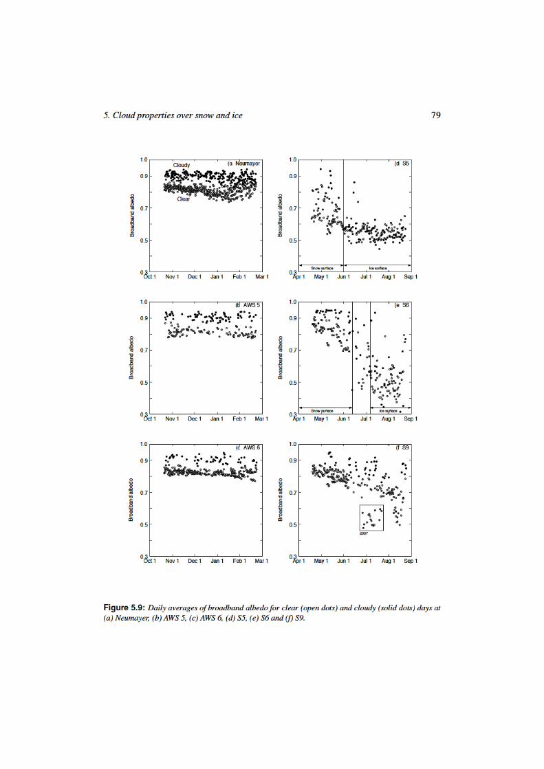
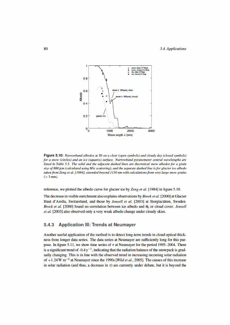
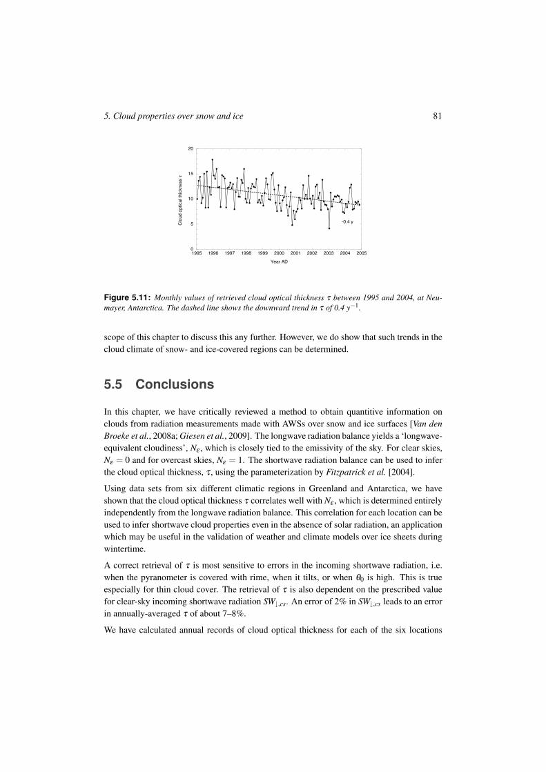
5. Cloud properties over snow and ice 81
0
5
10
15
20
1995 1996 1997 1998 1999 2000 2001 2002 2003 2004 2005
Clo
ud o
ptical th
ickness !
Year AD
-0.4 y
Figure 5.11: Monthly values of retrieved cloud optical thickness & between 1995 and 2004, at Neu-mayer, Antarctica. The dashed line shows the downward trend in & of 0.4 y"1.
scope of this chapter to discuss this any further. However, we do show that such trends in thecloud climate of snow- and ice-covered regions can be determined.
5.5 Conclusions
In this chapter, we have critically reviewed a method to obtain quantitive information onclouds from radiation measurements made with AWSs over snow and ice surfaces [Van denBroeke et al., 2008a; Giesen et al., 2009]. The longwave radiation balance yields a ‘longwave-equivalent cloudiness’, N+ , which is closely tied to the emissivity of the sky. For clear skies,N+ = 0 and for overcast skies, N+ = 1. The shortwave radiation balance can be used to inferthe cloud optical thickness, & , using the parameterization by Fitzpatrick et al. [2004].
Using data sets from six different climatic regions in Greenland and Antarctica, we haveshown that the cloud optical thickness & correlates well with N+ , which is determined entirelyindependently from the longwave radiation balance. This correlation for each location can beused to infer shortwave cloud properties even in the absence of solar radiation, an applicationwhich may be useful in the validation of weather and climate models over ice sheets duringwintertime.
A correct retrieval of & is most sensitive to errors in the incoming shortwave radiation, i.e.when the pyranometer is covered with rime, when it tilts, or when #0 is high. This is trueespecially for thin cloud cover. The retrieval of & is also dependent on the prescribed valuefor clear-sky incoming shortwave radiation SW+,cs. An error of 2% in SW+,cs leads to an errorin annually-averaged & of about 7–8%.
We have calculated annual records of cloud optical thickness for each of the six locations
82 5.5. Conclusions
considered in this study. It shows that both in Greenland and Antarctica, cloud become thin-ner and clear-sky conditions more frequent away from the coast. A smaller precipitable watercolumn at higher altitude and with lower temperatures can explain these findings. Moreover,& increases throughout the summer both in Antarctica and Greenland, which reduces theeffect that low ice albedos have on the shortwave radiation balance.
Three applications were presented to demonstrate the versatility of the method. Using & as aselection criterion, it is possible to distinguish between clear and cloudy days, and assess theinfluence of clouds on e.g. the radiation budget and snow and ice albedo. Although clouds doattenuate shortwave radiation due to reflection and absorption, the incoming solar radiation atthe surface is partly compensated for this loss by multiple reflections between the surface andthe cloud base. Averaged over all summer days, multiple reflection enhances SW+ by 18%(S5) to 29% (Neumayer) relative to the situation without multiple reflections. Furthermore,we have shown that over snow surfaces, albedo under cloudy sky is always higher than theclear-sky albedo, due to the ‘spectral effect’ of clouds. Over ice surfaces, this differenceceases, since the visible albedo of ice is so low that the ‘spectral effect’ that dominates oversnow is very weak over ice. As a third application, we detected a clear trend of decreasing &from the 1995–2004 Neumayer data series, consistent with a reported increase in incomingsolar radiation. The method is thus suitable to detect long-term trends in the optical propertiesof clouds over snow and ice.
The use of the methods presented in this chapter is not restricted to glaciers and ice sheets. Itcan be applied to any snow or ice surface, as long as radiation measurements are reasonablyreliable. This opens up possibilities to explore data records from seasonally snow-coveredregions in the Arctic. Although not tested here, the method could even be applicable toradiation data over any surface. For that, the coefficients derived by Fitzpatrick et al. [2004]should be rederived using spectral albedos typical for that surface.
6The energy budget of the
snowpack at Summit, Greenland
Summary
Measurements of the summer surface energy balance at Summit, Greenland, are presented(June 8 – July 20, 2007). These measurements serve as input to an energy balance model thatsearches for a surface temperature for which closure of all energy terms is achieved. A goodagreement between observed and modelled surface temperatures was found, with an aver-age difference of 0.45#C and an RMSE of 0.85#C. It turns out that penetration of shortwaveradiation into the snowpack plays a small but important role in correctly simulating snowtemperatures. After 42 days, snow temperatures in the first meter are 3.6–4.0#C higher com-pared to a model simulation without radiation penetration. Sensitivity experiments show thatthese results cannot be reproduced by tuning the heat conduction process alone, by varyingsnow density or snow diffusivity. We compared the two-stream radiation penetration calcu-lations with a sophisticated radiative transfer model and discuss the differences. The averagediurnal cycle shows that net shortwave radiation is the largest energy source (+61 W m"2 onaverage), net longwave radiation the largest energy sink ("42 W m"2). On average, subsur-face heat flux, sensible and latent heat fluxes are the remaining, small heat sinks ("5, "5 and"7 W m"2, respectively), although these are more important on a subdaily timescale.
This chapter is published as Kuipers Munneke, P., M. R. van den Broeke, C. H. Reijmer, M. M. Helsen, W.Boot, M. Schneebeli and K. Steffen (2009), The role of radiation penetration in the energy budget of the snowpackat Summit, Greenland, The Cryosphere, 3, 155-165.
83
84 6.1. Introduction
6.1 Introduction
The energy balance at the surface of a snowpack is given by
SWnet +LWnet +Hsen +Hlat + Gs = M (6.1)
(all terms in [W m"2]) where the net shortwave radiation, SWnet , is the sum of global short-wave radiation, SW+, and reflected radiation, SW,; net longwave radiation, LWnet , is the sumof downwelling longwave radiation, LW+, and upwelling longwave radiation, LW,; Hsen is theturbulent sensible heat flux, Hlat is turbulent latent heat flux, Gs is the subsurface heat flux atthe surface, and M is the amount of melt energy.
In the absence of meltwater percolation, the temperature distribution within the snowpack isgoverned mainly by heat conduction, which has a diffusive nature. Close to the surface, alsonon-diffusive processes take place, like subsurface penetration and subsequent absorption ofshortwave radiation [Colbeck, 1989b], wind pumping [Colbeck, 1989a], and latent heat trans-fer by subsurface water vapour transport [Albert and Shultz, 2002]. The latter two processesare known to play a role at high wind speeds. Earlier studies suggested that the subsurfaceheat production by penetration of shortwave radiation could be significant [Schlatter, 1972],leading to a ‘solid-state greenhouse’ [Matson and Brown, 1989], in which shortwave radia-tion is absorbed below the surface while longwave radiation is emitted at the surface. Later,it was shown that these studies overestimated this effect as they did not take into accountthe large variation of the extinction coefficient of snow with wavelength [Brandt and War-ren, 1993]. Hence, the latter authors concluded that subsurface heating in Antarctica mustbe very small. The importance of treating subsurface radiation spectrally is underlined byexperimental studies on subsurface radiation fluxes, e.g. by Meirold-Mautner and Lehning[2004] at Summit. Although it was shown that radiation penetration was overestimated pre-viously, Liston and Winther [2005] suggested that no less than 20% of the snow-covered areaof Antarctica experiences subsurface melt. Since most of this meltwater refreezes locally, theeffect on the mass balance of Antarctica is supposed to be small.
Although the effect was shown to be smaller than presumed before, it potentially affects thesubsurface temperature distribution, since energy is transferred below the surface more ef-ficiently than by conduction of heat from the surface layer alone. For ice, it was alreadydemonstrated that radiation penetration plausibly explains observed vertical temperature dis-tributions and vertical melt extent at several sites in the ablation zone of the Greenland icesheet [Van den Broeke et al., 2008b]. For snow, the influence of radiation penetration on theformation of depth hoar [Alley et al., 1990] and crystal growth [Colbeck, 1989b] has beenstudied in detail, although the latter did not use a spectral model. Absorption of radiationbelow the surface leads to strong snow temperature gradients just below the surface. For acorrect simulation of the effect of radiation penetration on snow temperature, it is thereforeimportant to use a sufficiently high resolution of the subsurface model [Dadic et al., 2008].
6. Energy budget at Summit 85
In this chapter, we present detailed and high-quality measurements of the energy budget ofthe snowpack during two summer months at Summit, Greenland, and show that subsurfaceabsorption of penetrated radiation plays an important role for the temperature distributionin the snowpack. In section 6.2 and 6.3, the data and energy balance model are presented;section 6.4 discusses the results, and the paper is concluded and summarized in section 6.5.
6.2 Data
In this section, we present data acquired in a period of 42 days from June 8 to July 20,2007, during the Summit Radiation Experiment (SURE 07), performed at the GreenlandEnvironmental Observatory at Summit (72o34’ N 38o28’ W, 3209 m a.s.l.), on top of theGreenland ice sheet.
A single-level automatic weather station (AWS) performed ventilated measurements of airtemperature Ta, air pressure p, relative humidity RH, and wind speed u at 3.85 m above thesurface. The specific humidity of air, q, is calculated from these data. Below the surface,subsurface snow temperatures Tsn,i were measured at depths zi using thermistor strings (0.20,0.30, 0.50, 0.75 and 1.00 m) and thermocouples (spaced 0.02 m up to 0.10 m). AWS datawere stored as 5-minute averages on a Campbell CR10X datalogger.
The radiation components of the surface energy balance were measured with a separate in-stallation equipped with high-quality sensors for long- and shortwave radiation. SWnet wasmeasured with a pair of Kipp & Zonen (K&Z) CM21 pyranometers (the upward-looking onebeing ventilated); LWnet was measured using K&Z CG4 pyrgeometers (again, the upward-looking one being ventilated). The radiation data were stored as 1-minute averages.
The upward-looking pyranometer regularly suffered from rime accretion during clear nights,which was removed manually every morning around 7:15am local time (09:15 GMT). SW+data suspected to be corrupted by rime were replaced by parameterized data by linearly in-terpolating the albedo during the period of the data gap and using SW,.
We compared the K&Z CG4 LWnet measurements with data acquired by Eppley PrecisionInfrared Radiometers (PIR) at the nearby candidate-BSRN radiation station [Baseline SurfaceRadiation Network, Ohmura et al., 1998]. It was found that the CG4 LW, measurementswere systematically overestimated (3.5 W m"2 on average, peaking at 5–7 W m"2 duringdaytime). Contrary to the BSRN measurements, the CG4 sensor measuring LW, was notventilated and its measurements were affected by window heating, i.e. heating of the sensordome by reflected solar radiation. Since the thermal conduction between the dome and thethermopile measuring sensor housing temperature is near-perfect, the thermopile gets toowarm and the calculated LW -fluxes too high. Window heating is less of a problem for theventilated upward-facing CG4 (1.9 W m"2 difference with the Eppley PIR on average), butthe BSRN Eppley PIR LW+ measurements are preferred as they are shielded from direct solar
86 6.3. The energy balance model
radiation. Comparison of the SW -fluxes with those from the BSRN site showed that ourmeasurements have less scatter (presumably due to regular removal of accreted rime). In theremainder of this manuscript, we will therefore use the K&Z CM21 SW -fluxes from our setupand the Eppley PIR LW -fluxes from the candidate-BSRN station.
The sensible heat flux was measured directly with a Campbell CSAT3 sonic anemometerat a frequency of 20 Hz, and 5-minute averages were stored on a separate Campbell CR10Xdatalogger. The sonic anemometer was fitted with a Campbell Chromel Constantan 75 micronthermocouple for temperature measurements. Hsen,obs can be deduced from the measurementsof vertical wind velocity and potential temperature variations w& and # &, using the flux-profilerelation
Hsen,obs = ,acp(w&# &)zson , (6.2)
where ,a is the density of air, cp the specific heat capacity of dry air, and zson the sonicanemometer measurement height.
The latent heat flux was not measured directly, but rather computed using the bulk aerody-namic method as explained in section 6.3.
6.3 The energy balance model
For the calculation of the energy budget of the snowpack, the model by Van den Broeke et al.[2005] was used [see also Van As et al., 2005a; Giesen et al., 2008]. The model calculates theenergy fluxes of a skin layer without heat capacity, it employs the bulk aerodynamic methodfor turbulent fluxes (see section 6.3.1), and it calculates the subsurface temperature profileusing the one-dimensional heat-transfer equation (section 6.3.3). Using SWnet , LW+ and theAWS measurements as input, the energy balance in equation 6.1 is solved iteratively in orderto find a value for Ts for which the energy budget is closed. As we will see later, this iterativeprocedure makes the model very robust, and less susceptible to errors in input data: since allfluxes are interrelated, and a change in Ts has opposing effects on different fluxes, errors inthe input are strongly damped. This was also demonstrated in an error analysis by Van Aset al. [2005a]. The model has a time step of 1 minute.
6.3.1 Turbulent fluxes
In the energy balance model, the turbulent fluxes are calculated using
Hsen = ,acpu0#0 (6.3)
Hlat = ,aLv,su0q0, (6.4)
6. Energy budget at Summit 87
where Lv,s is latent heat of vapourization or sublimation, depending on the surface temper-ature Ts. The surface friction velocity u0, and the turbulent scaling parameters for temper-ature #0 and specific humidity q0, are computed using the bulk method – a method thatexploits Monin-Obukhov similarity theory for wind, temperature and moist profiles in thesurface layer, and the following assumptions at the surface: at the surface roughness lengthfor momentum z0,u, wind velocity u(z0,u) = 0; at roughness length for temperature z0,T , airtemperature Ta(z0,T ) = Ts; and at roughness length for moisture z0,q, the air is saturated:q(z0,q) = qsat(z0,q). With the Monin-Obukhov length L,
L =u20
-g/# [#0+0.62#q0], (6.5)
u0, #0 and q0 can be expressed using measurements of u, Ta and q at measurement levels zu,zT and zq:
u0 =-u(zu)
ln&
zuz0,u
'")m
( zuL)+)m
( z0,uL
) (6.6)
#0 =-(Ta(zT )"Ts)
ln&
zTz0,T
'")h
( zTL
)+)h
( z0,TL
) (6.7)
q0 =-(q(zq)"qsat(z0,q))
ln&
zqz0,q
'")h
( zqL)+)h
( z0,qL
) . (6.8)
In the above equations, - = 0.4 is the Von Karman constant; )m,h are vertically-integratedstability correction functions taken from Holtslag and de Bruin [1988] for stable conditionsand Dyer [1974] for unstable conditions (which occur regularly during daytime at Summit[Cullen and Steffen, 2001; Cullen et al., 2007]). Roughness length for momentum, z0,u, istaken constant at 3.8% 10"4 m, derived from sonic anemometer measurements. Values forz0,T and z0,q are calculated following Andreas [1987]. Since u0 (and #0 and q0) requires thecalculation of L, which is in turn dependent on u0 (and #0 and q0), the turbulent fluxes aresolved iteratively.
6.3.2 Radiation penetration
The model includes a module to calculate subsurface radiation penetration of shortwave radi-ation following the method presented by [Brandt and Warren, 1993]. The model is identicalto the one used in Van den Broeke et al. [2008b]. This module employs the two-streamapproach from Schlatter [1972], giving analytical functions for attenuation of shortwave ra-diation per wavelength. The module calculates radiation in 118 wavelength bands coveringthe solar spectrum, and uses Mie scattering coefficients derived from Warren [1984], updatedwith values from Warren et al. [2006] for the UV and visible wavelength range. The two-
88 6.3. The energy balance model
stream analytical functions require a constant snow density ,sn,rp and effective snow grainradius re. The grid spacing for the radiation penetration calculations is 0.001 m. Results onthis grid are interpolated onto the 0.01 m grid used for the subsurface calculations (see section6.3.3). Increasing the grid resolution any further did not affect the results.
Energy released by radiation penetration in the snowpack is added to the appropriate sub-surface model layers, and the total amount of penetrated radiation Q is subtracted from thesurface skin layer. Equation 6.1, which is valid for the surface layer, formally becomes
SWnet +LWnet +Hsen +Hlat +Gs"Q = M (6.9)
For an infinitesimally thin surface layer, SWnet = Q and these terms would cancel for thesurface layer. Because of the discrete nature of the model numerics however, the surfacelayer energy budget retains the shape of equation 6.9.
The hypothesized effect of incorporating radiation penetration is that energy is released belowthe surface, enabling a more rapid warming of the snowpack.
6.3.3 Subsurface flux
To obtain the subsurface heat flux G, a subsurface module is included in the model, whichcalculates the one-dimensional heat-transfer equation on a 0.01 m grid up to a depth of 20 m,beyond which G is assumed to be zero. The model results are insensitive to grid size smallerthan 0.01 m. It was already pointed out by Dadic et al. [2008] that modelling of subsurfaceprocesses should be done at a sufficiently high resolution, as the temperature gradient attainslarge values. The snow density profile, ,sn(z) is prescribed using measurements from severalsnow pits, and thus decoupled from the constant density required for the radiation penetrationcalculations. In each snow pit, we collected one pair of density profiles, spaced about 0.30 mapart to account for horizontal variations and to reduce the measurement error. In total, 7pairs of density profiles have been collected with an approximate resolution of 0.02 m upto a depth of 1.0 m, which were interpolated in time to account for temporal variations, andinterpolated onto the 0.01 m subsurface grid. Below 1.0 m, density is taken constant at 400 kgm"3.
Thermal conductivity of snow, ksn, is prescribed as a function of ,sn(z) (in kg m"3), followingAnderson [1976]:
ksn = 0.021+2.5& ,sn
1000
'2(6.10)
The specific heat capacity of ice, cp,ice, is a function of Tsn(z). The vertical snow temperatureprofile was initialized using measurements typical for June at Summit [Hoch, 2005], scaledin the uppermost meter with our own measurements of Tsn.
The subsurface heat flux at the surface is denoted as Gs, and calculated using the modeltemperature gradient at the surface. To compare our energy budget calculations with previous
6. Energy budget at Summit 89
studies [Cullen and Steffen, 2001; Hoch, 2005] that did not explicitly distinguish betweensubsurface heat fluxes by diffusion and subsurface radiation penetration, we will present theircombined effects as Gs using model snow temperatures [Hoch, 2005]:
Gs ="n"1
%j=1
$Tsn(z j)/$t +$Tsn(z j+1)/$t2
· cp,ice, j ·,sn, j · (z j " z j+1) (6.11)
The temperatures at the subsurface grid are used, and at z = 0 the observed Ts,obs is pre-scribed, making n = 2001. By calculating Gs in this way, the snowpack is regarded as abox containing a certain amount of heat, which is closed at the bottom (no heat exchange atthe lower boundary) — the subsurface heat flux at the surface is thus assumed to equal therate of change of the total heat storage in the snowpack, whether caused by heat diffusion orsubsurface radiation absorption. In the terminology of the equations presented above:
Gs = Gs"Q (6.12)
assuming that other subsurface heat sources or sinks (e.g. wind pumping or water vapourtransport) are negligible. In that case, Gs is the same quantity as in equation 6.1.
6.4 Results and comparison with measurement data
As described before, the AWS measurements, as well as the measurements of SWnet and LW+,drive the energy balance model. Its performance can be assessed by means of three criteria:
1. Calculated surface temperature Ts,mod and observed surface temperature, Ts,obs, derivedfrom LW, measurements, should be in good agreement
2. Calculated Hsen and the directly measured Hsen,obs from the sonic anemometer shouldbe in good agreement,
3. The evolution of subsurface temperatures Tsn,i in the model should agree with observedsnow temperatures.
In this section, we present model results in the optimal setting, perform a sensitivity analysis,and demonstrate the role of radiation penetration in the energy budget of the snowpack.
6.4.1 Results
The optimal results of the energy balance model, determined by the best performance on theabove-mentioned criteria, are shown in figure 6.1, which compares Ts,mod and Ts,obs (criterion1). This calculation will be referred to as the ‘optimal run’.
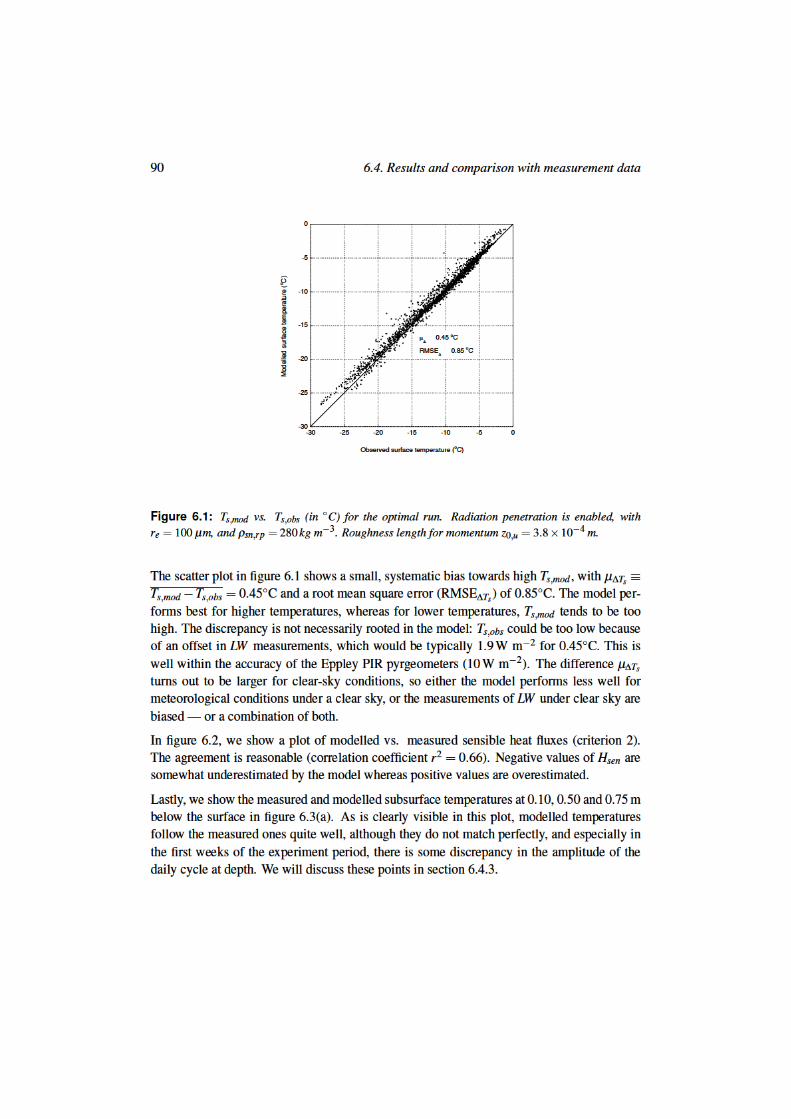
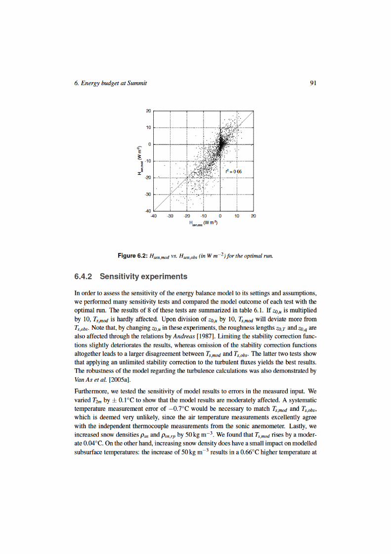
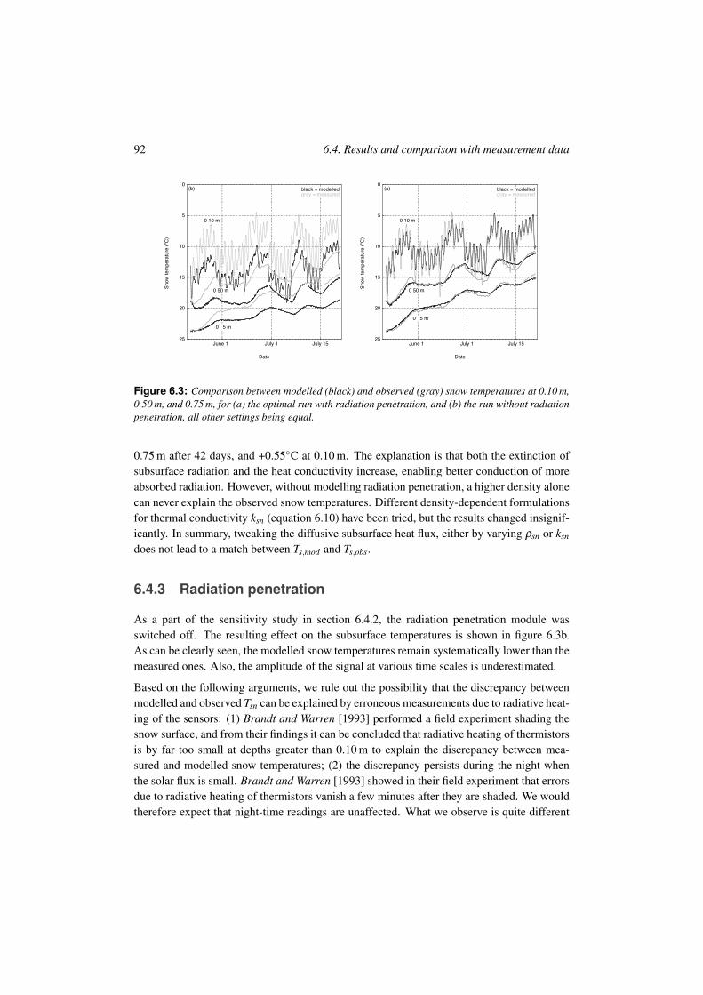
92 6.4. Results and comparison with measurement data
25
20
15
10
5
0
June 1 July 1 July 15
Sn
ow
te
mp
era
ture
(oC
)
Date
black = modelledgray = measured
(b)
0 10 m
0 50 m
0 5 m
25
20
15
10
5
0
June 1 July 1 July 15
Sn
ow
te
mp
era
ture
(oC
)Date
(a) black = modelledgray = measured
0 10 m
0 50 m
0 5 m
Figure 6.3: Comparison between modelled (black) and observed (gray) snow temperatures at 0.10 m,0.50 m, and 0.75 m, for (a) the optimal run with radiation penetration, and (b) the run without radiationpenetration, all other settings being equal.
0.75 m after 42 days, and +0.55#C at 0.10 m. The explanation is that both the extinction ofsubsurface radiation and the heat conductivity increase, enabling better conduction of moreabsorbed radiation. However, without modelling radiation penetration, a higher density alonecan never explain the observed snow temperatures. Different density-dependent formulationsfor thermal conductivity ksn (equation 6.10) have been tried, but the results changed insignif-icantly. In summary, tweaking the diffusive subsurface heat flux, either by varying ,sn or ksn
does not lead to a match between Ts,mod and Ts,obs.
6.4.3 Radiation penetration
As a part of the sensitivity study in section 6.4.2, the radiation penetration module wasswitched off. The resulting effect on the subsurface temperatures is shown in figure 6.3b.As can be clearly seen, the modelled snow temperatures remain systematically lower than themeasured ones. Also, the amplitude of the signal at various time scales is underestimated.
Based on the following arguments, we rule out the possibility that the discrepancy betweenmodelled and observed Tsn can be explained by erroneous measurements due to radiative heat-ing of the sensors: (1) Brandt and Warren [1993] performed a field experiment shading thesnow surface, and from their findings it can be concluded that radiative heating of thermistorsis by far too small at depths greater than 0.10 m to explain the discrepancy between mea-sured and modelled snow temperatures; (2) the discrepancy persists during the night whenthe solar flux is small. Brandt and Warren [1993] showed in their field experiment that errorsdue to radiative heating of thermistors vanish a few minutes after they are shaded. We wouldtherefore expect that night-time readings are unaffected. What we observe is quite different
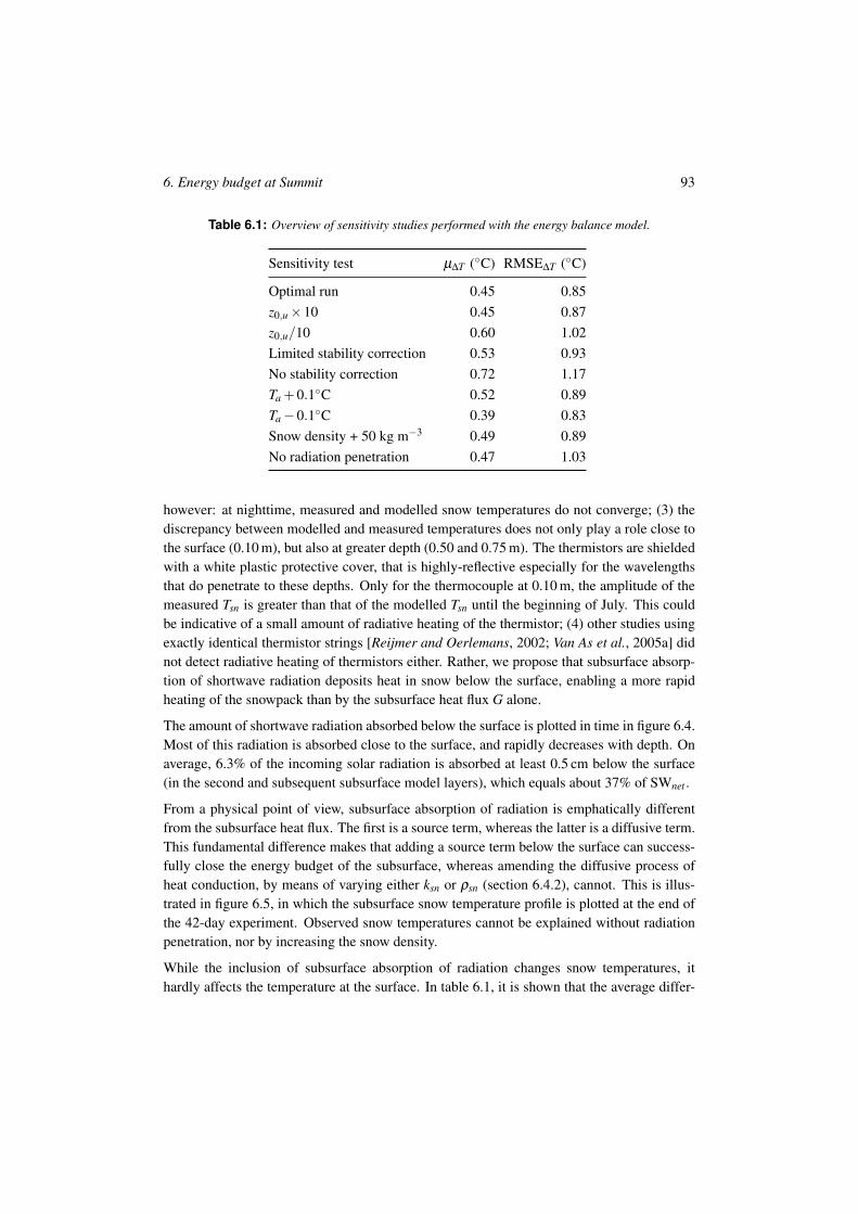
6. Energy budget at Summit 93
Table 6.1: Overview of sensitivity studies performed with the energy balance model.
Sensitivity test µ$T (#C) RMSE$T (#C)
Optimal run 0.45 0.85z0,u%10 0.45 0.87z0,u/10 0.60 1.02Limited stability correction 0.53 0.93No stability correction 0.72 1.17Ta +0.1#C 0.52 0.89Ta"0.1#C 0.39 0.83Snow density + 50 kg m"3 0.49 0.89No radiation penetration 0.47 1.03
however: at nighttime, measured and modelled snow temperatures do not converge; (3) thediscrepancy between modelled and measured temperatures does not only play a role close tothe surface (0.10 m), but also at greater depth (0.50 and 0.75 m). The thermistors are shieldedwith a white plastic protective cover, that is highly-reflective especially for the wavelengthsthat do penetrate to these depths. Only for the thermocouple at 0.10 m, the amplitude of themeasured Tsn is greater than that of the modelled Tsn until the beginning of July. This couldbe indicative of a small amount of radiative heating of the thermistor; (4) other studies usingexactly identical thermistor strings [Reijmer and Oerlemans, 2002; Van As et al., 2005a] didnot detect radiative heating of thermistors either. Rather, we propose that subsurface absorp-tion of shortwave radiation deposits heat in snow below the surface, enabling a more rapidheating of the snowpack than by the subsurface heat flux G alone.
The amount of shortwave radiation absorbed below the surface is plotted in time in figure 6.4.Most of this radiation is absorbed close to the surface, and rapidly decreases with depth. Onaverage, 6.3% of the incoming solar radiation is absorbed at least 0.5 cm below the surface(in the second and subsequent subsurface model layers), which equals about 37% of SWnet .
From a physical point of view, subsurface absorption of radiation is emphatically differentfrom the subsurface heat flux. The first is a source term, whereas the latter is a diffusive term.This fundamental difference makes that adding a source term below the surface can success-fully close the energy budget of the subsurface, whereas amending the diffusive process ofheat conduction, by means of varying either ksn or ,sn (section 6.4.2), cannot. This is illus-trated in figure 6.5, in which the subsurface snow temperature profile is plotted at the end ofthe 42-day experiment. Observed snow temperatures cannot be explained without radiationpenetration, nor by increasing the snow density.
While the inclusion of subsurface absorption of radiation changes snow temperatures, ithardly affects the temperature at the surface. In table 6.1, it is shown that the average differ-
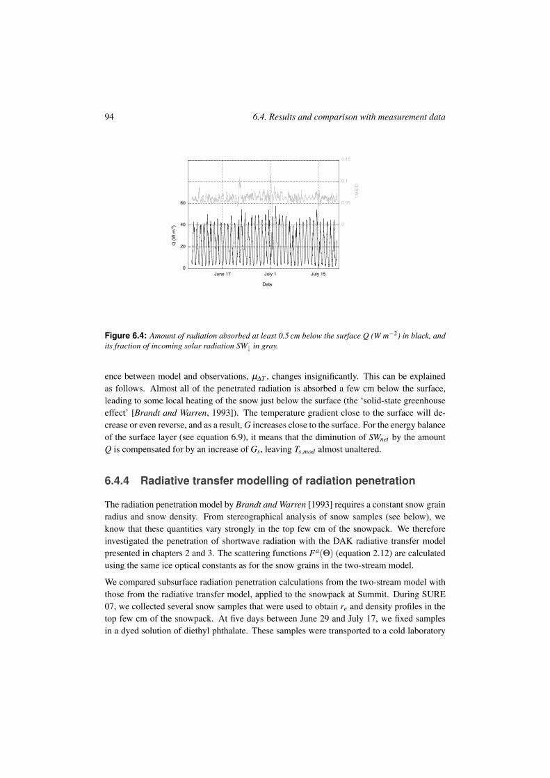
94 6.4. Results and comparison with measurement data
0
20
40
60
0
0.05
0.1
0.15
June 17 July 1 July 15
Q (
W m
-2)
Q/S
W!
Date
Figure 6.4: Amount of radiation absorbed at least 0.5 cm below the surface Q (W m"2) in black, andits fraction of incoming solar radiation SW+ in gray.
ence between model and observations, µ$T , changes insignificantly. This can be explainedas follows. Almost all of the penetrated radiation is absorbed a few cm below the surface,leading to some local heating of the snow just below the surface (the ‘solid-state greenhouseeffect’ [Brandt and Warren, 1993]). The temperature gradient close to the surface will de-crease or even reverse, and as a result, G increases close to the surface. For the energy balanceof the surface layer (see equation 6.9), it means that the diminution of SWnet by the amountQ is compensated for by an increase of Gs, leaving Ts,mod almost unaltered.
6.4.4 Radiative transfer modelling of radiation penetration
The radiation penetration model by Brandt and Warren [1993] requires a constant snow grainradius and snow density. From stereographical analysis of snow samples (see below), weknow that these quantities vary strongly in the top few cm of the snowpack. We thereforeinvestigated the penetration of shortwave radiation with the DAK radiative transfer modelpresented in chapters 2 and 3. The scattering functions Fa(#) (equation 2.12) are calculatedusing the same ice optical constants as for the snow grains in the two-stream model.
We compared subsurface radiation penetration calculations from the two-stream model withthose from the radiative transfer model, applied to the snowpack at Summit. During SURE07, we collected several snow samples that were used to obtain re and density profiles in thetop few cm of the snowpack. At five days between June 29 and July 17, we fixed samplesin a dyed solution of diethyl phthalate. These samples were transported to a cold laboratory
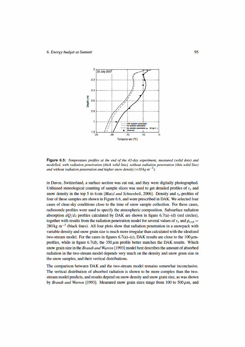
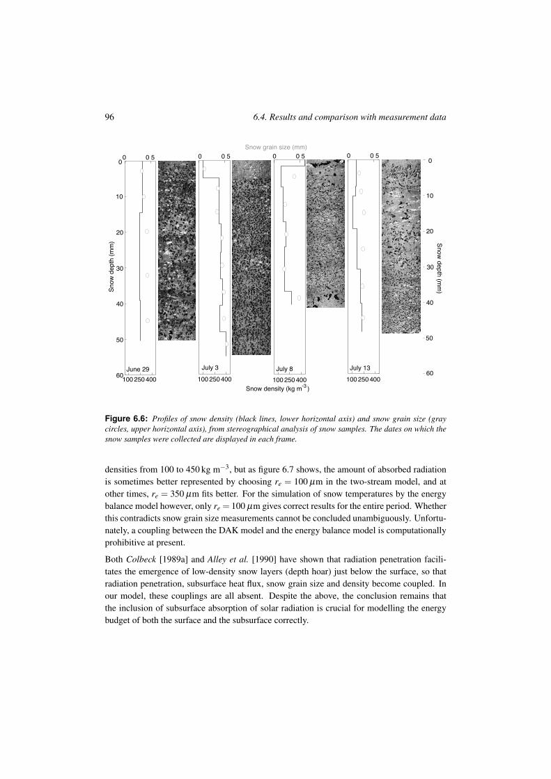
96 6.4. Results and comparison with measurement data
Snow density (kg m-3 )
Snow grain size (mm)
Snow
dep
th (m
m)
100 250 400
0
10
20
30
40
50
60
0 0 5
June 29100 250 400
0 0 5
July 3
100 250 400
0 0 50
10
20
30
40
50
60July 13
100 250 400
0 0 5
July 8
Snow depth (m
m)
Figure 6.6: Profiles of snow density (black lines, lower horizontal axis) and snow grain size (graycircles, upper horizontal axis), from stereographical analysis of snow samples. The dates on which thesnow samples were collected are displayed in each frame.
densities from 100 to 450 kg m"3, but as figure 6.7 shows, the amount of absorbed radiationis sometimes better represented by choosing re = 100 µm in the two-stream model, and atother times, re = 350 µm fits better. For the simulation of snow temperatures by the energybalance model however, only re = 100 µm gives correct results for the entire period. Whetherthis contradicts snow grain size measurements cannot be concluded unambiguously. Unfortu-nately, a coupling between the DAK model and the energy balance model is computationallyprohibitive at present.
Both Colbeck [1989a] and Alley et al. [1990] have shown that radiation penetration facili-tates the emergence of low-density snow layers (depth hoar) just below the surface, so thatradiation penetration, subsurface heat flux, snow grain size and density become coupled. Inour model, these couplings are all absent. Despite the above, the conclusion remains thatthe inclusion of subsurface absorption of solar radiation is crucial for modelling the energybudget of both the surface and the subsurface correctly.
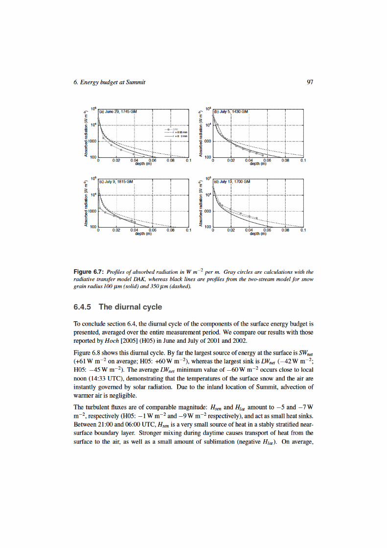
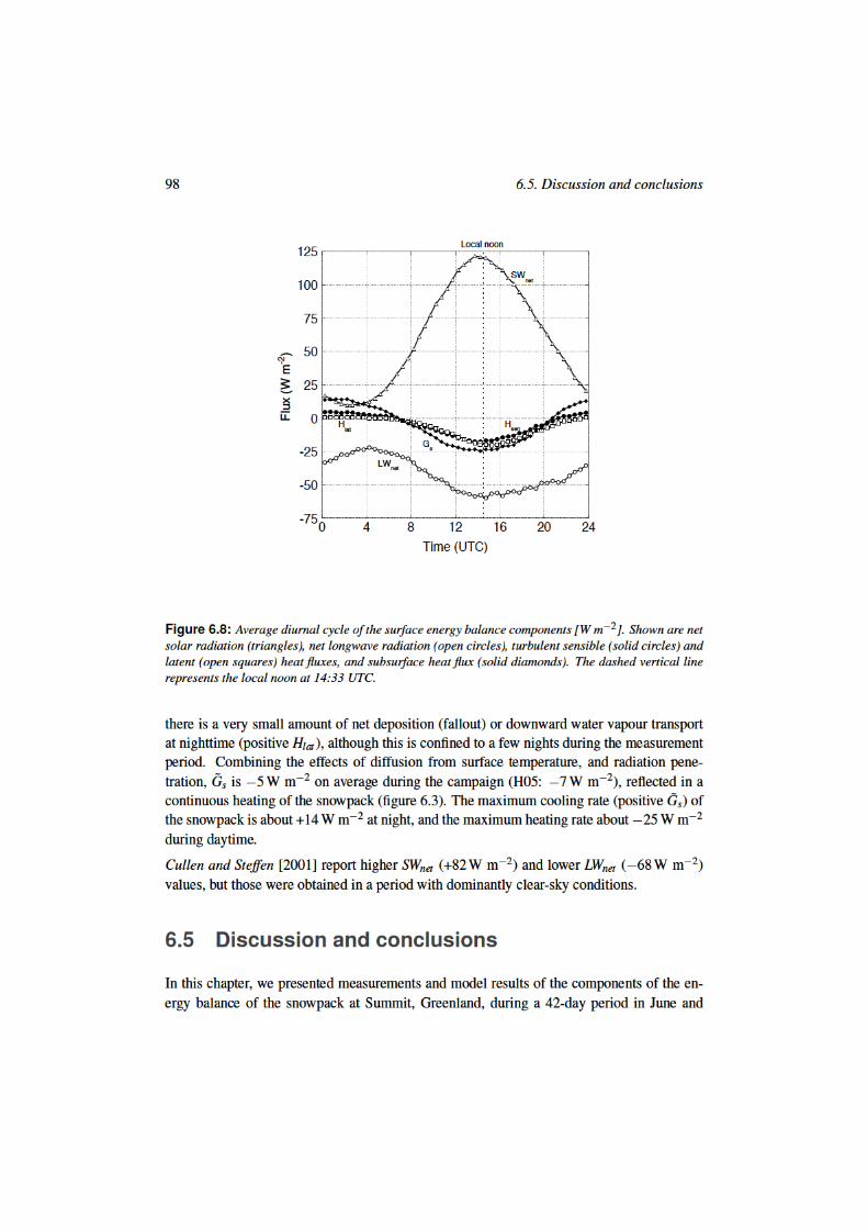
6. Energy budget at Summit 99
July 2007. The energy balance model simulates observed snow surface temperatures well,although on average modelled and observed snow surface temperatures differ by 0.45 #C. Theenergy balance model was shown to be somewhat sensitive to the prescribed surface rough-ness length, and to small errors in input 2-meter temperatures. Furthermore, the subsurfacetemperatures slightly depend on the prescribed snow density profile, but the effect is small ingeneral. It was found that observed subsurface temperatures could not be reproduced withoutincluding a radiation penetration term in the energy balance model. Although observed snowgrain radii in the top 5 cm range from 100 to 500 µm, subsurface temperatures could only bereconstructed using a radius of 100 µm. The use of a sophisticated radiative transfer modelcould not solve this possible discrepancy unambiguously, although for 3 out of 4 test cases,the 100 µm-profiles fit the radiative transfer model calculations best. Nevertheless, we arguedthat the inclusion of a radiation penetration term is required to close the energy budget of thesnowpack satisfyingly.
A natural question that comes to mind is why subsurface absorption of shortwave radiationis apparently important at Summit, while it has not been reported to be necessary to closethe energy budget at other locations, either those like Hardangerjøkulen, a small, temper-ate ice cap in Norway [Giesen et al., 2008], or in similar circumstances like the AntarcticPlateau [Van den Broeke et al., 2004c; Van As et al., 2005a]. In the case of measurements onHardangerjøkulen and melting glaciers in general, the energy fluxes from melt and internalrefreezing, and the associated model uncertainties, largely exceed those of absorbed subsur-face radiation or the subsurface heat flux, making it hard to assess what importance radiationpenetration has in the heating of the snowpack. Before the start of the melt season at Hardan-gerjøkulen, the modelled snow temperatures are in fact lower than the measured ones [R.H. Giesen, personal communication, 2009], suggesting that radiation penetration has someeffect on snow temperature, but this might also be attributed to some intermittent meltwaterpercolation and refreezing, not captured by the model. Considering that, on glaciers, snowgrains can become large, snow can get wet or bare ice can appear at the surface, the magni-tude of absorbed subsurface radiation will be larger than at Summit, but still smaller than meltenergy fluxes. Regarding the Antarctic Plateau measurements, it could be that a combinationof larger snow density [Van As et al., 2005a] and smaller snow grains (chapter 4) makes theeffect much less apparent, but this requires further study.

7Spectral snow albedo and snow
grain size
Summary
In this chapter, we present measurements of spectral snow albedo, carried out at Summit,Greenland. Concurrently, we collected snow samples that were stereologically analyzed andthat provided high-resolution vertical profiles of snow grain size. These profiles were used inthe radiative transfer model DAK to calculate spectral albedo of snow. We show that there is agood agreement between the radiative transfer model results and the observations of spectralalbedo. Thus, it is experimentally shown that the optical properties of a natural snowpack aredetermined by its physical properties. For correctly modelling spectral albedo, it is necessaryto include a thin ($0.5–1.0 mm) top layer of small snow grains, as suggested in previousliterature. These small layers are also present in the observed snow profiles, stressing theneed to measure snow grain size at millimeter resolution close to the surface.
101
102 7.1. Introduction
7.1 Introduction
In chapter 4, we saw that the broadband albedo (!) of a snow surface is highly variable, evenin the dry-snow zones of ice sheets. Observed values are typically between 0.78 and 0.84under clear skies [Van den Broeke et al., 2004a], and even higher when clouds are present. Inchapter 4, I suggested that for dry snow, spatial and temporal variations in clear-sky albedoare mainly due to variability in the size of the surface snow grains. Spatial variations in snowgrain size on Antarctica are demonstrated by a MODIS (Moderate resolution Imaging Spec-trometer) snow grain size product [Scambos et al., 2007], showing small grains on the Plateauand larger grains in coastal areas. The resulting variations in albedo have important impli-cations for the energy budget of the snow surface: absorbed solar radiation is proportionalto 1"! , and so for high-albedo surfaces, a small change in albedo has a profound effect onthe amount of absorbed radiation available for heating of the snowpack. Knowledge of thespectral optical properties of natural snow surfaces is therefore important.
It has been well established theoretically that snow microstructure has an effect on the op-tical properties of the snowpack, as I discussed in chapter 3. Wiscombe and Warren [1980]put forward a model based on Mie theory, that clearly demonstrates that larger snow grainsdecrease broadband albedo due to increased scattering of radiation in the forward direction.Flanner and Zender [2006] link the evolution of snow microstructure (i.e. changes in shapeand size of snow crystals) to changes in broadband surface albedo.
The computation of the optical properties of irregularly-shaped snow crystals is difficult,but a versatile approximation is to replace the snow crystals with spherical snow grains thathave the same volume-to-surface (V/S) ratio [Dobbins and Jizmagian, 1966; Warren, 1982,chapter 3 of this thesis]. The success of this approach has been underlined by Grenfell andWarren [1999] and Neshyba et al. [2003] for cylindrical and hexagonal-plate shaped crystals.Essentially, this approximation allows one to convert the specific surface area (SSA) [m"1]of any crystal shape mixture to an optically-equivalent snow grain radius re [m]. SSA isdefined as the ratio between surface area and volume of the ice constituting the snow grains[Warren, 1982; Legagneux and Domine, 2005], and re is the radius of the equivalent V/Sspheres that replace the actual snow crystals [Mitchell, 2002]. Measuring SSA (and thusre) is therefore a useful way to link snow microstructure observations with radiative transfermodel calculations using spherical particles.
Recently, there has been a considerable advance in fast and quantitative methods to obtainthe SSA of snow samples. Among these methods are contact spectroscopy using the iceabsorption feature at 1030 nm [Painter et al., 2007], an integrating-sphere measurement ofspectral albedo at 1310 and 1550 nm [Gallet et al., 2009] and a combination of stereologyand near-infrared (NIR) photography [Matzl and Schneebeli, 2006]. Apart from these opticalmethods, Legagneux et al. [2002] put forward a method based on the adsorption of methanein snow samples to determine SSA.
7. Snow albedo at Summit 103
There are numerous accounts in literature on measurements of spectral snow albedo [Kuhnand Siogas, 1978; Grenfell and Perovich, 1984; Grenfell et al., 1994; Zhou et al., 2003; Wut-tke et al., 2006], many of which were performed in the Antarctic. Fewer are the attempts tocompare observed spectral snow albedo with radiative transfer calculations over a snowpackusing concurrent observations of snow grain size. Grenfell et al. [1994] compare measure-ments of albedo throughout the shortwave spectrum with traditional snow grain size mea-surements. Domine et al. [2006] combine methane-adsorption measurements of SSA withspectral albedo measurements at 4 wavelengths between 1310 and 2260 nm. However, theseoptical measurements are done on snow samples, not above a natural snow surface. It meansthat, for the optical characterization of the snow, the natural snow is disturbed in order toobtain a sample volume. The same is true for the study by Gallet et al. [2009].
In this chapter, we combine field observations of spectral snow albedo with highly detailedobservations of SSA (and using the equal V/S approximation also re) in the first few centime-ters of the snowpack. Both the optical characterization of the snow and the determination ofSSA is done on a virtually undisturbed snow surface.
In section 7.2, we will present the data and methods that are used for this study, and explainthe corrections that have been applied to the data. In the subsequent section, we will showexamples of spectral albedo, show the consistency of the results, and compare the spectralalbedo measurements with radiative transfer calculations. In section 7.4, the results are dis-cussed and this chapter is concluded.
7.2 Data and methods
The data used in this study were collected during the 42-day Summit Radiation Experiment2007 (SURE ’07) in June and July 2007 at the Greenland Environmental Observatory atSummit (72#34’ N 38#28’ W, 3209 m a.s.l.), on top of the Greenland Ice Sheet (see section1.6).
7.2.1 Spectroradiometer
Spectral snow albedos were collected using an ASD (Analytical Spectral Devices) FieldSpecPro FR spectroradiometer, covering the solar spectrum between 350 and 2500 nm in 1 nmintervals. The spectral resolution (full width at half-maximum) is 3 nm at 700 nm and 10 nmat 1400 and 2100 nm. Hemispherical spectral irradiances [W m"2 nm"1] were recorded usinga white diffuser plate that guides radiation from a half-sphere into a fiber optical cable to thespectroradiometer. Incoming spectral irradiance E"+ was measured by leveling the diffuserplate horizontally, viewing the sky, whereas reflected spectral irradiance E", was measured
104 7.2. Data and methods
in the opposite direction, facing the snow surface. Using the definition
!" =E",E"+
, (7.1)
spectral albedo !" as a function of wavelength " is calculated. Each measurement of E"is an average of 15 consecutive scans. Pairs of E"+ and E", measurements were collectedby alternating upward- and downward-looking measurements, and five of these pairs werecombined to obtain one average spectrum of E"+, E",, and !" . So all in all, an averagealbedo spectrum !" is based on 2%5%15 = 150 scans, 75 of which are E"+, and 75 are E",.Recording one such average albedo spectrum takes about 10 minutes. A measurement error%E(" ) is determined using the standard deviation of these 75 spectra. The measurement errorin albedo %!(" ) is calculated from %E+(" ) and %E,(" ), assuming that these are independent.
Between 16 June and 16 July 2007, 112 of these averaged spectra were collected duringwidely varying illumination conditions, under clear and overcast skies, and with the solarzenith angle #0 ranging from 49.1# to 83.0#. The change of the solar zenith angle #0 duringthe measurements is corrected for.
7.2.2 Spectroradiometer corrections
Following Grenfell et al. [1994], we applied a wavelength-dependent correction to the irradi-ance spectra for the non-ideal cosine response of the diffuser plate. If the measured responseis S" (#), the response correction is given as f" (#) = S" (#)/cos# . For direct incident radi-ation arriving from solar zenith angle #0, the correction becomes
Edir"+ (true) =
Edir"+ (observed)
f" (#0). (7.2)
Also for diffuse irradiance, a correction C" is necessary, such that
Edi f"+ (true) = C" Edi f
"+ (observed) (7.3)
Assuming that the diffuse irradiance is isotropic, C" is given as
C" =*
2" (/2
0f" (#)sin# cos#d#
+"1
. (7.4)
See Grenfell et al. [1994] for a more complete derivation. Considering that a fraction Fdi f" of
the incoming irradiance is diffuse, and that Fdi f" + Fdir
" = 1, the true spectral albedo can be
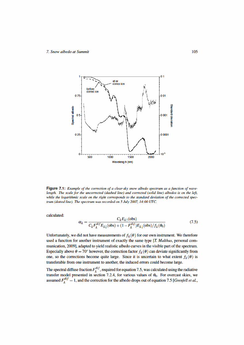
106 7.2. Data and methods
1994].
Next, we corrected for the fraction of the field-of-view of the diffuser plate that was occupiedby the instrument casing during measurements of E" ,, [see Wuttke et al., 2006, their equa-tion 4]. For each measurement of the reflected spectral irradiance, we assumed an occupiedfraction of the field-of-view of 0.018, and a wavelength-independent albedo of the instrumentcasing of 0.20. This correction leads to slightly higher albedos (up to +0.01) in the visiblepart of the spectrum.
Despite the correction for the non-ideal cosine response of the diffuser plate, measurementsunder clear sky with #0 > 70# feature visible albedos > 1 and larger uncertainties of spectralalbedo in the NIR region due to very small irradiances. The high visible albedos suggestthat the cosine response correction f" (#) is not adequately known for high # . Therefore,clear-sky measurements for #0 > 70# are discarded. Furthermore, cloudy-sky measurementsfor which the irradiance was insufficiently stable (e.g. due to rapidly fluctuating cloud opticalthickness) were discarded as well. Out of the 112 averaged spectra, we retain 18 spectraunder a completely clear sky, 29 spectra under skies with 1/8 cloud cover (not blocking thesun), and 11 spectra under homogeneous cloud cover. Cloud cover was determined by eye,and checked with observations from a Total Sky Imager.
An example of a clear-sky spectral albedo measurement before and after corrections is shownin figure 7.1. Note that irradiance measurements turned out not to be reliable between 2120and 2380 nm, due to a low signal-to-noise ratio of the spectroradiometer. Spectral albedocurves are therefore shown up to 2120 nm. The corrections are most prominent in the visibleand decrease towards the NIR. Also shown in figure 7.1 is the measurement error %!(" ),which steadily grows between 500 and 2200 nm. Local maxima occur around 1350 and1850 nm, where absorption by water vapour causes larger uncertainties in E"+.
7.2.3 Snow grain size profiles
During SURE ’07, we collected several snow samples that were used to obtain SSA anddensity profiles in the top few cm of the snowpack (see also sections 1.6 and 6.4.4). At fivedays between June 29 and July 17, we fixed samples in a dyed solution of diethyl phthalate.These samples were transported to a cold laboratory in Davos, Switzerland, a surface sectionwas cut out, and they were digitally photographed. Unbiased stereological counting of sampleslices [Matzl, 2006] was used to get detailed profiles of snow grain size and snow densityin the top 5 to 6 cm. Invoking the equal-V/S theory, the inverse of SSA is proportional tothe optically-equivalent snow grain radius re [m]. For the top 5 mm, the resolution of thestereological grid was increased by a factor of 3 (nine times more grid points) to capturevariability very close to the surface. The results are independent on the resolution of thestereological grid.
In figure 7.2, we show the uppermost millimeters of the vertical snow grain profiles taken on
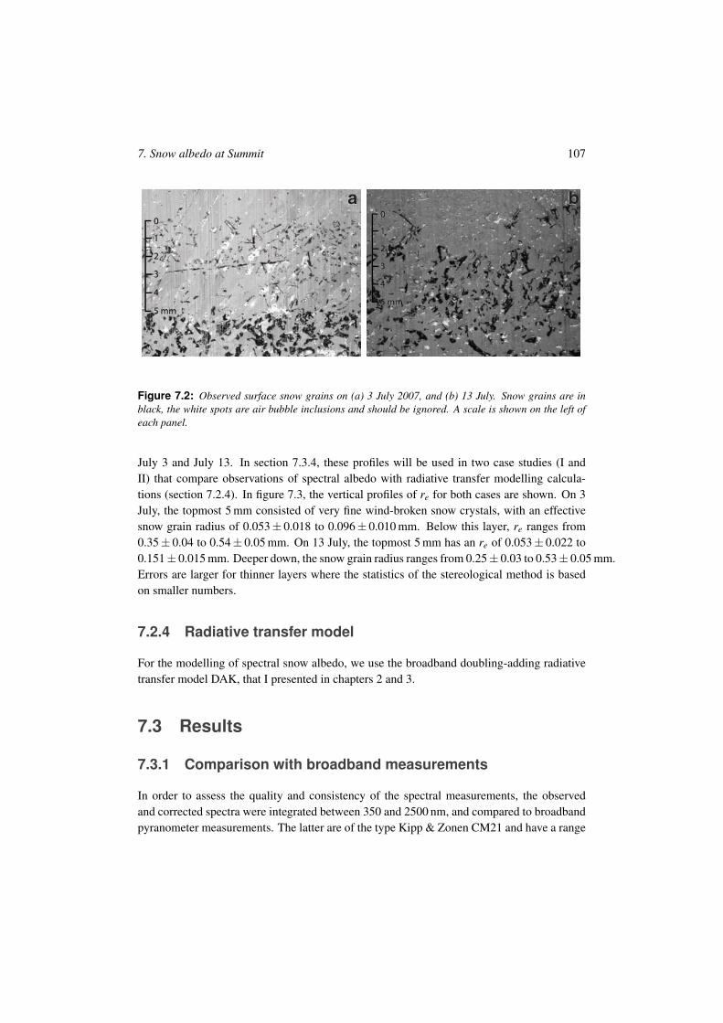
7. Snow albedo at Summit 107
a ba b
Figure 7.2: Observed surface snow grains on (a) 3 July 2007, and (b) 13 July. Snow grains are inblack, the white spots are air bubble inclusions and should be ignored. A scale is shown on the left ofeach panel.
July 3 and July 13. In section 7.3.4, these profiles will be used in two case studies (I andII) that compare observations of spectral albedo with radiative transfer modelling calcula-tions (section 7.2.4). In figure 7.3, the vertical profiles of re for both cases are shown. On 3July, the topmost 5 mm consisted of very fine wind-broken snow crystals, with an effectivesnow grain radius of 0.053± 0.018 to 0.096± 0.010 mm. Below this layer, re ranges from0.35± 0.04 to 0.54± 0.05 mm. On 13 July, the topmost 5 mm has an re of 0.053± 0.022 to0.151± 0.015 mm. Deeper down, the snow grain radius ranges from 0.25± 0.03 to 0.53± 0.05 mm.Errors are larger for thinner layers where the statistics of the stereological method is basedon smaller numbers.
7.2.4 Radiative transfer model
For the modelling of spectral snow albedo, we use the broadband doubling-adding radiativetransfer model DAK, that I presented in chapters 2 and 3.
7.3 Results
7.3.1 Comparison with broadband measurements
In order to assess the quality and consistency of the spectral measurements, the observedand corrected spectra were integrated between 350 and 2500 nm, and compared to broadbandpyranometer measurements. The latter are of the type Kipp & Zonen CM21 and have a range
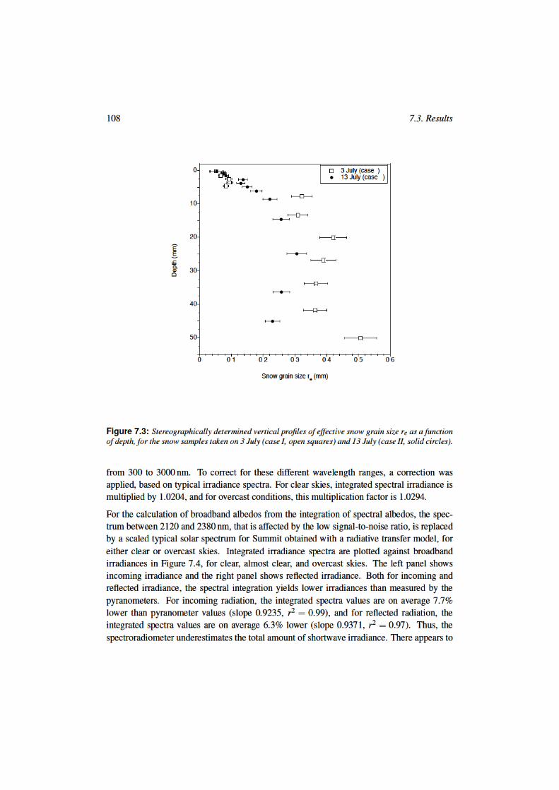
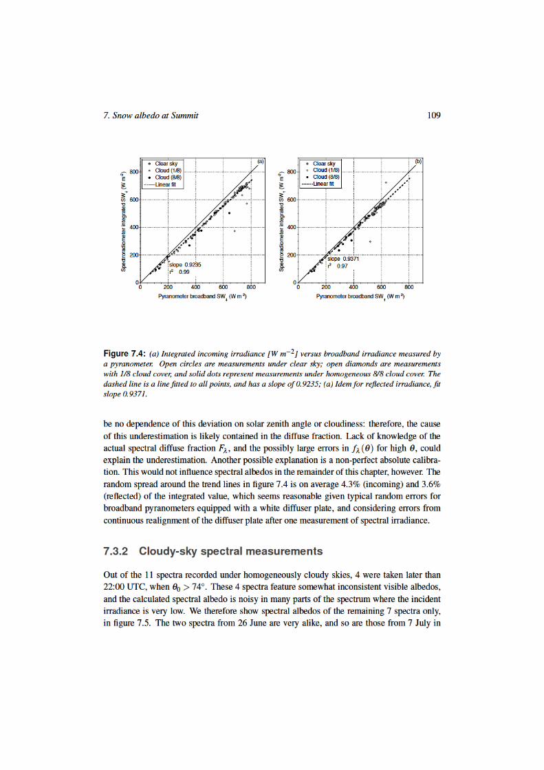
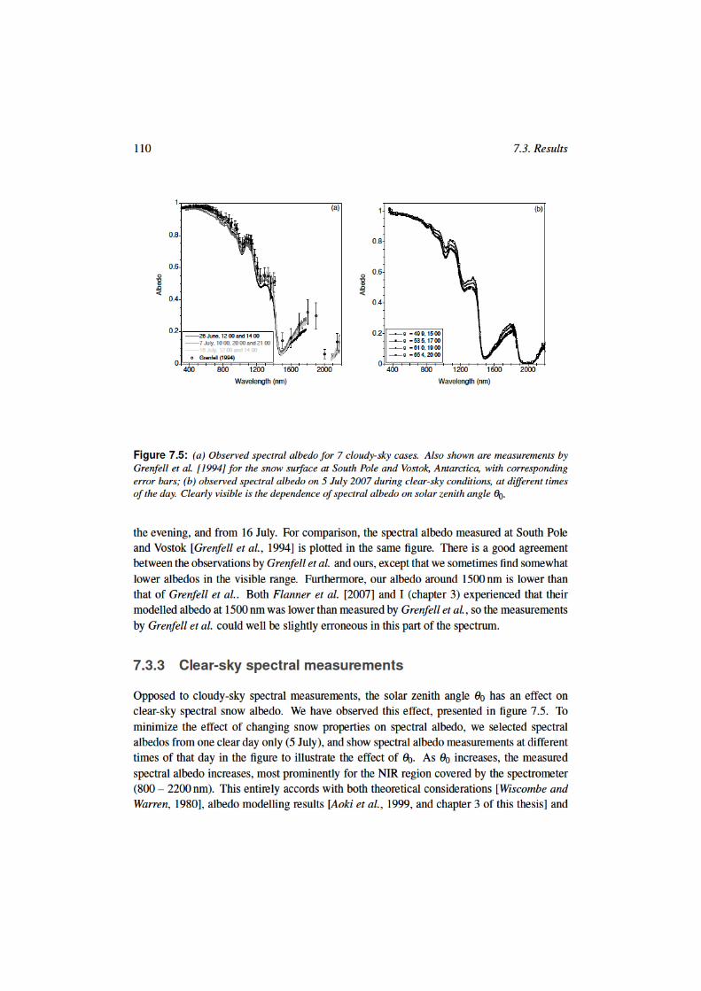
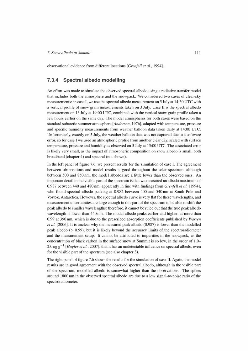
7. Snow albedo at Summit 111
observational evidence from different locations [Grenfell et al., 1994].
7.3.4 Spectral albedo modelling
An effort was made to simulate the observed spectral albedo using a radiative transfer modelthat includes both the atmosphere and the snowpack. We considered two cases of clear-skymeasurements: in case I, we use the spectral albedo measurement on 5 July at 14:30 UTC witha vertical profile of snow grain measurements taken on 3 July. Case II is the spectral albedomeasurement on 13 July at 19:00 UTC, combined with the vertical snow grain profile taken afew hours earlier on the same day. The model atmospheres for both cases were based on thestandard subarctic summer atmosphere [Anderson, 1976], adapted with temperature, pressureand specific humidity measurements from weather balloon data taken daily at 14:00 UTC.Unfortunately, exactly on 5 July, the weather balloon data was not captured due to a softwareerror, so for case I we used an atmospheric profile from another clear day, scaled with surfacetemperature, pressure and humidity as observed on 5 July at 15:00 UTC. The associated erroris likely very small, as the impact of atmospheric composition on snow albedo is small, bothbroadband (chapter 4) and spectral (not shown).
In the left panel of figure 7.6, we present results for the simulation of case I. The agreementbetween observations and model results is good throughout the solar spectrum, althoughbetween 500 and 850 nm, the model albedos are a little lower than the observed ones. Animportant detail in the visible part of the spectrum is that we measured an albedo maximum of0.987 between 440 and 480 nm, apparently in line with findings from Grenfell et al. [1994],who found spectral albedo peaking at 0.982 between 400 and 540 nm at South Pole andVostok, Antarctica. However, the spectral albedo curve is very flat for these wavelengths, andmeasurement uncertainties are large enough in this part of the spectrum to be able to shift thepeak albedo to smaller wavelengths: therefore, it cannot be ruled out that the true peak albedowavelength is lower than 440 nm. The model albedo peaks earlier and higher, at more than0.99 at 390 nm, which is due to the prescribed absorption coefficients published by Warrenet al. [2006]. It is unclear why the measured peak albedo (0.987) is lower than the modelledpeak albedo (> 0.99), but it is likely beyond the accuracy limits of the spectroradiometerand the measurement setup. It cannot be attributed to impurities in the snowpack, as theconcentration of black carbon in the surface snow at Summit is so low, in the order of 1.0–2.0 ng g"1 [Hagler et al., 2007], that it has an undetectable influence on spectral albedo, evenfor the visible part of the spectrum (see also chapter 3).
The right panel of figure 7.6 shows the results for the simulation of case II. Again, the modelresults are in good agreement with the observed spectral albedo, although in the visible partof the spectrum, modelled albedo is somewhat higher than the observations. The spikesaround 1800 nm in the observed spectral albedo are due to a low signal-to-noise ratio of thespectroradiometer.
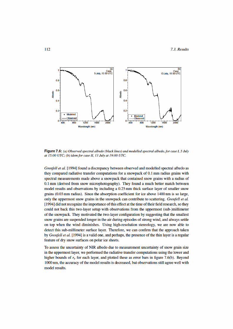
7. Snow albedo at Summit 113
7.4 Discussion and conclusions
In section 7.3, we have demonstrated the ability of the radiative transfer model to simulateobserved spectral albedo curves closely. We have shown experimentally that there is a directlink between the microstructure of the surface snow and the observed spectral surface albedo.Of key importance for a good agreement between spectral albedo measurements over a snowsurface and modelling results is the availability of vertical profiles of snow grain size at asufficiently detailed resolution, in the order of 1 mm. Below, we will discuss possible sourcesof error in our study, and discuss the possibilities and limitations of existing SSA-retrievalmethods to relate spectral albedo measured over a snow surface to the snow microstructure.
A possible source of error in case I is that there are two full days between the snow sampling(3 July) and the spectral albedo observations (5 July). It is possible that the snow surface haschanged during these days, but on the other hand, the weather was sunny, cold, almost wind-less and without snowfall during these two days, implying that no wind crust has formed,no small grains were deposited on top, no snow was eroded away, and that little snow meta-morphism has taken place. If anything, sublimation due to turbulent latent heat fluxes ofapproximately "15 W m"1 during the day helped to maintain small snow grains near thesurface (chapter 6). We argue that the vertical profile of snow grains must have been muchalike on 3 and 5 July, at least within the error bounds shown in figure 7.3.
Stereological analysis of snow crystals in very thin layers poses the problem that these layersbecome as thin as the typical surface roughness of a natural snow surface. While the calcula-tion of SSA and re is independent of the (somewhat arbitrary) definition of the snow surfacein the stereology images, the snow density needed for the radiative transfer calculations isnot. We assume however that the impact of this error on the radiation calculations is notlarger than the uncertainty of the modelled spectral albedo caused by the uncertainty in thedetermination of snow grain size (the error bars in figure 7.6).
While technological advance has triggered the development of a number of techniques tomeasure SSA by optical means, not all of these techniques can provide the high resolutionneeded for a good quantification of the optical properties of a snow surface. While the stere-ological method employed here can in principle handle the < 1 mm resolution as shown inthis study [Matzl and Schneebeli, 2006], the method by Painter et al. [2007] can resolve 2 cmlayers, and that by Gallet et al. [2009] has a resolution that is dictated by how thin a layercan be collected undisturbed into one snow sample. For those methods to become even moreuseful in the characterization of the optical properties of natural snow surfaces, it remains achallenge in future development to increase the resolution even further.

116 Bibliography
Colbeck, S. C. (1989b), Snow-crystal growth with varying surface temperatures and radiation penetration, J.Glaciol., 35(119), 23–29.
Cullen, N. J., and K. Steffen (2001), Unstable near-surface boundary conditions in summer on top of the Greenlandice sheet, Geophys. Res. Lett., 28(23), 4491–4493.
Cullen, N. J., K. Steffen, and P. D. Blanken (2007), Nonstationarity of turbulent heat fluxes at Summit, Greenland,Boundary-Layer Meteorol., 122, 439–455.
Dadic, R., M. Schneebeli, M. Lehning, M. A. Hutterli, and A. Ohmura (2008), Impact of the microstructure ofsnow on its temperature: A model validation with measurements from Summit, Greenland, J. Geophys. Res. (D),113(D14303), doi:10.1029/2007JD009562.
De Haan, J. F., P. B. Bosma, and J. W. Hovenier (1987), The adding method for multiple scattering calculations ofpolarized light, Astron. Astrophys., 183, 371–391.
De Rooij, W. A., and C. C. A. H. van der Stap (1984), Expansion of Mie scattering matrices in generalized sphericalfunctions, Astron. Astrophys., 131, 237–248.
Deepak, A., and H. E. Gerber (Eds.) (1983), WCP-55. World Climate Research report of the experts meeting onaerosols and their climatic effects., Williamsburg, Virginia, 28-30 March 1983.
Dobbins, R. A., and G. S. Jizmagian (1966), Optical scattering cross sections for polydispersions of dielectricspheres, J. Opt. Soc. Am., 56, 1345–1350.
Domine, F., R. Salvatori, L. Legagneux, R. Salzano, M. Fily, and R. Casacchia (2006), Correlation between thespecific surface area and the short wave infrared (SWIR) reflectance of snow, Cold Reg. Sci. Technol., 46, 60–68.
Dubovik, O., A. Smirnov, B. N. Holben, M. D. King, Y. J. Kaufman, T. F. Eck, and I. Slutsker (2000), Accuracyassessments of aerosol optical properties retrieved from Aerosol Robotic Network (AERONET) sun and skyradiance measurements, J. Geophys. Res. (D), 105(D8), 9791–9806.
Durr, B., and R. Philipona (2004), Automatic cloud amount detection by surface longwave downward radiationsmeasurements, J. Geophys. Res. (D), 109, doi:10.1029/2004JD004182.
Dyer, A. J. (1974), A review of flux-profile relationships, Boundary-Layer Meteorol., 7, 363–372.Dyurgerov, M., and M. F. Meier (2005), Glaciers and the changing Earth system: a 2004 snapshot, Occasional
paper 58, 118 pp., Institute of Arctic and Alpine Research, Boulder, CO.Ettema, J., M. R. van den Broeke, E. van Meijgaard, W. J. van de Berg, J. L. Bamber, J. E. Box, and R. C. Bales
(2009), Higher surface mass balance of the Greenland ice sheet revealed by high-resolution climate modelling,Geophys. Res. Lett., 36, L12,501, doi:10.1029/2009GL038110.
Fettweis, X., J. P. van Ypersele, H. Gallee, F. Lefebre, and W. Lefebvre (2007), The 1979–2005 Greenland icesheet melt extent from passive microwave data using an improved version of the melt retrieval XPGR algorithm,Geophys. Res. Lett., 34, L05,502, doi:10.1029/2006GL028787.
Fitzpatrick, M. F., R. E. Brandt, and S. G. Warren (2004), Transmission of solar radiation by clouds over snow andice surfaces: a parameterization in terms of optical depth, solar zenith angle, and surface albedo, J. Clim., 17,266–275.
Flanner, M. G., and C. S. Zender (2006), Linking snowpack microphysics and albedo evolution, J. Geophys. Res.(D), 111, D12,208, doi:10.1029/2005JD006834.
Flanner, M. G., C. S. Zender, J. T. Randerson, and P. J. Rasch (2007), Present-day climate forcing and response fromblack carbon in snow, J. Geophys. Res. (D), 112, D11,202, doi:10.1029/2006JD008003.
Gallet, J.-C., F. Domine, C. S. Zender, and G. Picard (2009), Rapid and accurate measurement of the specific surfacearea of snow using infrared reflectance at 1310 and 1550 nm, The Cryosphere Discuss., 3(1), 33–75.
Gay, M., M. Fily, C. Genthon, M. Frezzotti, H. Oerter, and J. G. Winther (2002), Snow grain-size measurements inAntarctica, J. Glaciol., 48(163), 527–535.
Giesen, R. H., M. R. van den Broeke, J. Oerlemans, and L. M. Andreassen (2008), Surface energy balance in theablation zone of Midtdalsbreen, a glacier in southern Norway: interannual variability and the effect of clouds, J.Geophys. Res. (D), 113, D21,111, doi:10.1029/2008JD010390.
Giesen, R. H., L. M. Andreassen, M. R. van den Broeke, and J. Oerlemans (2009), Comparison of the meteorologyand surface energy balance at Storbreen and Midtdalsbreen, two glaciers in southern Norway, The Cryosphere, 3,57–74.
Grenfell, T. C., and G. A. Maykut (1977), The optical properties of ice and snow in the Arctic basin, J. Glaciol.,
Bibliography 117
18(80), 445–463.Grenfell, T. C., and D. K. Perovich (1984), Spectral albedos of sea ice and incident solar irradiance in the southern
Beaufort Sea, J. Geophys. Res., 89, 3573–3580.Grenfell, T. C., and S. G. Warren (1999), Representation of a nonspherical ice particle by a collection of independent
spheres for scattering and absorption of radiation, J. Geophys. Res. (D), 104(D24), 31,697–31,709.Grenfell, T. C., S. G. Warren, and P. C. Mullen (1994), Reflection of solar radiation by the Antarctic snow surface at
ultraviolet, visible, and near-infrared wavelengths, J. Geophys. Res. (D), 99(D9), 18,669–18,684.Greuell, W., and J. Oerlemans (2004), Narrowband-to-broadband albedo conversion for glacier ice and snow: equa-
tions based on modeling and ranges of validity of the equations, Rem. Sens. Environ., 89, 95–105.Greuell, W., W. H. Knap, and C. J. P. P. Smeets (1997), Elevational changes in meteorological variables along a
midlatitude glacier during summer, J. Geophys. Res. (D), 102(D22), 25,941–25,954.Griggs, J. A., and J. L. Bamber (2008), Assessment of cloud cover characteristics in satellite datasets and reanalysis
products for Greenland, J. Clim., 21, 1837–1849.Gueymard, C. A. (2001), Parameterized transmittance model for direct beam and circumsolar spectral irradiance,
Solar Energy, 71(5), 325–346.Gueymard, C. A. (2004), The sun’s total and spectral irradiance for solar energy applications and solar radiation
models, Solar Energy, 76, 423–453.Hagler, G. S. W., M. H. Bergin, E. A. Smith, and J. E. Dibb (2007), A summer time series of particulate carbon in
the air and snow at Summit, Greenland, J. Geophys. Res. (D), 112, D21,309, doi:10.1029/2007JD008993.Hays, J. D., J. Imbrie, and N. J. Shackleton (1976), Variations in the Earth’s orbit: pacemaker of the ice ages, Science,
194(4270), 1121–1132.Henzing, J. S., W. H. Knap, P. Stammes, A. Apituley, J. B. Bergwerff, D. P. J. Swart, G. P. A. Kos, and H. M. ten
Brink (2004), Effect of aerosols on the downward shortwave irradiances at the surface: measurements versuscalculations with MODTRAN 4.1, J. Geophys. Res. (D), 109, D14,204, doi:10.1029/2003JD004142.
Hess, M., R. B. A. Koelemeijer, and P. Stammes (1998a), Scattering matrices of imperfect hexagonal ice crystals, J.Quant. Spectrosc. Radiat. Transfer, 60(3), 301–308.
Hess, M., P. Koepke, and I. Schult (1998b), Optical properties of aerosols and clouds: the software package OPAC,Bull. Am. Meteorol. Soc., 79(2), 831–844.
Hoch, S. W. (2005), Radiative flux divergence in the surface boundary layer. A study based on observations atSummit, Greenland, Ph.D. thesis, Swiss Federal Institute of Technology, Zurich.
Hoffmann, P. F., A. J. Kaufman, G. P. Halverson, and D. P. Schrag (1998), A Neoproterozoic Snowball Earth,Science, 281, 1342–1346.
Holtslag, A. A. M., and H. A. R. de Bruin (1988), Applied modelling of the night-time surface energy balance overland, J. Appl. Meteorol., 27, 689–704.
Hovenier, J. W., C. van der Mee, and H. Domke (2004), Transfer of polarized light in planetary atmospheres, KluwerAcademic Publishers, Dordrecht, The Netherlands.
IPCC (2007), Climate change 2007: The physical science basis. Contribution of working groups I to the fourthassessment report of the Intergovernmental Panel on Climate Change.
Jonsell, U., R. Hock, and B. Holmgren (2003), Spatial and temporal variations in albedo on Storglaciaren, Sweden,J. Glaciol., 49(164), 59–68.
Karkas, E., H. Granberg, K. Kanto, K. Rasmus, C. Lavoie, and M. Lepparanta (2002), Physical properties of theseasonal snow cover in Dronning Maud Land, East Antarctica, Ann. Glaciol., 34, 89–94.
Kato, S., T. P. Ackerman, J. H. Mather, and E. E. Clothiaux (1999), The k-distribution method and correlated-kapproximation for a shortwave radiative transfer model, J. Quant. Spectrosc. Radiat. Transfer, 62, 109–121.
Knap, W. H., C. H. Reijmer, and J. Oerlemans (1999), Narrowband to broadband conversion of Landsat-TM glacieralbedos, Int. J. Remote Sens., 20(10), 2091–2110.
Knap, W. H., L. C. Labonnote, G. Brogniez, and P. Stammes (2005), Modeling total and polarized reflectances ofice clouds: evaluation by means of POLDER and ATSR-2 measurements, Appl. Opt., 44(19), 4060–4073.
Kneizys, F. X., E. P. Shettle, L. W. Abreu, J. H. Chetwynd, G. P. Anderson, W. O. Gallery, J. E. A. Selby, and S. A.Clough (1988), A users guide to LOWTRAN7, Air Force Geophysics Laboratory, Hanscom AFB, MA 01731.
Konig-Langlo, G., and A. Herber (1996), The meteorological data of the Neumayer Station (Antarctica) for 1992,
118 Bibliography
1993 and 1994, Ber. Polarforsch. 187, Alfred Wegener Institute for Polar and Marine Research, Bremerhaven.Konig-Langlo, G., J. C. King, and P. Pettre (1998), Climatology of the three coastal Antarctic stations Dumont
d’Urville, Neumayer, and Halley, J. Geophys. Res. (D), 103(D9), 10,935–10,946.Konzelmann, T., R. S. W. van de Wal, W. Greuell, R. Bintanja, E. A. C. Henneken, and A. Abe-Ouchi (1994),
Parameterization of global and longwave incoming radiation for the Greenland Ice Sheet, Glob. Plan. Change, 9,143–164.
Kuhn, M., and L. Siogas (1978), Spectroscopic studies at McMurdo, South Pole, and Siple stations during the australsummer 1977-78, Antarct. J. US, 13, 178–179.
Lacis, A. A., and V. Oinas (1991), A description of the correlated k distribution method for modeling nongraygaseous absorption, thermal emission, and multiple scattering in vertically inhomogeneous atmospheres, J. Geo-phys. Res. (D), 96(D5), 9027–9063.
Legagneux, L., and F. Domine (2005), A mean field model of the decrease of the specific surface area of dry snowduring isothermal metamorphism, J. Geophys. Res. (F), 110, F04,011, doi:10.1029/2004JF000181.
Legagneux, L., A. Cabanes, and F. Domine (2002), Measurement of the specific surface area of 176 snow samplesusing methane adsorption at 77 K, J. Geophys. Res. (D), 107(D17), 4335, doi:10.1029/2001JD001016.
Legagneux, L., A. S. Taillandier, and F. Domine (2006), Grain growth theories and the isothermal evolution of thespecific surface area of snow, J. Appl. Phys., 95(11), 6175–6184.
Liljequist, G. H. (1956), Energy exchange of an Antarctic snow field: Short-wave radiation (Maudheim 71#03’S, 10#56’ W), in Norwegian-British-Swedish Antarctic Expedition, 1949-52, Scientific Results, vol. 2, part 1A,Norsk Polarinstitutt, Oslo.
Liou, K. N. (2002), An introduction to atmospheric radiation, 2nd ed., Academic Press Inc., San Diego, USA.Liston, G. E., and J. G. Winther (2005), Antarctic surface and subsurface snow and ice melt fluxes, J. Clim., 18,
1469–1481.Long, C. N., and T. P. Ackerman (2000), Identification of clear skies from broadband pyranometer measurements
and calculation of downwelling shortwave cloud effects, J. Geophys. Res. (D), 105(D12), 15,609–15,626.Macke, A., J. Mueller, and E. Raschke (1996), Single scattering properties of atmospheric ice crystals, J. Atmos.
Sci., 53(19), 2813–2825.Mahesh, A., V. P. Walden, and S. G. Warren (2001), Ground-based infrared remote sensing of cloud properties over
the Antarctic plateau. Part II: cloud optical depths and particle sizes, J. Appl. Meteorol., 40, 1279–1294.Marty, C., and R. Philipona (2000), The clear-sky index to separate clear-sky from cloudy-sky situations in climate
research, Geophys. Res. Lett., 27(17), 2649–2652.Matson, D. L., and R. H. Brown (1989), Solid-state greenhouses and their implications for icy satellites, Icarus,
77(1), 67–81.Matzl, M. (2006), Quantifying the stratigraphy of snow profiles, Ph.D. thesis, Swiss Federal Institute of Technology,
Zurich.Matzl, M., and M. Schneebeli (2006), Measuring specific surface area of snow by near-infrared photography, J.
Glaciol., 52(179), 558–564.Meirold-Mautner, I., and M. Lehning (2004), Measurements and model calculations of the solar shortwave fluxes in
snow on Summit, Greenland, Ann. Glaciol., 38, 279–284.Meyers, T. P., and R. F. Dale (1983), Predicting daily insolation with hourly cloud height and coverage, J. Clim.
Appl. Meteorol., 22, 537–545.Michalsky, J. J., G. P. Anderson, J. Barnard, J. Delamare, C. Gueymard, S. Kato, P. Kiedron, A. McComiskey,
and P. Ricchiazzi (2006), Shortwave radiative closure studies from clear skies during the Atmospheric Ra-diation Measurement 2003 Aerosol Intensive Observation Period, J. Geophys. Res. (D), 111, D14S20, doi:10.1029/2005JD006341.
Milankovic, M. (1930), Mathematische Klimalehre und Astronomische Theorie der Klimaschwankungen. Handbuchder Klimalogie Band 1, Borntrager, Berlin.
Mishchenko, M. I. (2008), Multiple scattering, radiative transfer, and weak localization in discrete random media:unified microphysical approach, Rev. Geophys., 46.
Mishchenko, M. I., L. D. Travis, and A. A. Lacis (2006), Multiple scattering of light by particles: radiative transferand coherent backscattering, Cambridge University Press, Cambridge, UK.
Bibliography 119
Mitchell, D. L. (2002), Effective diameter in radiation transfer: General definition, applications, and limitations, J.Atmos. Sci., 59, 2330–2346.
Neshyba, S. P., T. C. Grenfell, and S. G. Warren (2003), Representation of a nonspherical ice particle by a collectionof independent spheres for scattering and absorption of radiation: 2. Hexagonal columns and plates, J. Geophys.Res. (D), 108(D15), doi:10.1029/2002JD003302.
Nolin, A. W., and J. Dozier (2000), A hyperspectral method for remotely sensing the grain size of snow, Rem. Sens.Environ., 74(2), 207–216.
Oerlemans, J., R. H. Giesen, and M. R. van den Broeke (2009), Retreating alpine glaciers: increased melt rates dueto accumulation of dust (Vadret da Morteratsch, Switzerland), J. Glaciol., 55(192), in press.
Ohmura, A., et al. (1998), Baseline Surface Radiation Network (BSRN/WCRP): new precision radiometry for cli-mate research, Bull. Am. Meteorol. Soc., 79(10), 2115–2136.
Painter, T. H., N. P. Molotch, M. Cassidy, M. G. Flanner, and K. Steffen (2007), Contact spectroscopy for determi-nation of stratigraphy of snow optical grain size, J. Glaciol., 53(180), 121–127.
Potter, J. F. (1970), The delta function approximation in radiative transfer theory, J. Atmos. Sci., 27, 943–949.Reijmer, C. H., and J. Oerlemans (2002), Temporal and spatial variability of the surface energy balance in Dronning
Maud Land, East Antarctica, J. Geophys. Res. (D), 107(D24), 4759–4770.Reijmer, C. H., E. van Meijgaard, and M. R. van den Broeke (2005), Evaluation of temperature and wind over
Antarctica in a Regional Atmospheric Climate Model using 1 year of automatic weather station data and upperair observations, J. Geophys. Res. (D), 110, doi:10.1029/2004JD005234.
Ricchiazzi, P., C. Gautier, and D. Lubin (1995), Cloud scattering optical depth and local surface albedo in the Antarc-tic: Simultaneous retrieval using ground-based radiometry, J. Geophys. Res. (D), 100(D10), 21,091–21,104.
Rignot, E., J. L. Bamber, M. R. van den Broeke, C. Davis, Y. Li, W. J. van de Berg, and E. van Meijgaard (2008),Recent Antarctic ice mass loss from radar interferometry and regional climate modelling, Nat. Geosci., 1, 106–110.
Rusin, N. P. (1961), Meteorological and radiational regime of Antarctica, Tech. rep., Israel program for scientifictranslations, Jerusalem.
Scambos, T. A., T. M. Haran, M. A. Fahnestock, T. H. Painter, and J. Bohlander (2007), MODIS-based Mosaicof Antarctica (MOA) data sets: continent-wide surface morphology and snow grain size, Rem. Sens. Environ.,111(2-3), 242–257.
Schlatter, T. W. (1972), The local surface energy balance and subsurface temperature regime in Antarctica, J. Appl.Meteorol., 11(10), 1048–1062.
Schneider, S. H., and R. E. Dickinson (1976), Parameterization of fractional cloud amounts in climatic models: theimportance of modeling multiple reflections, J. Appl. Meteorol., 15, 1050–1056.
Shepherd, A., and D. Wingham (2007), Recent sea-level contributions of the Antarctic and Greenland ice sheets,Science, 315, 1529–1532.
Shi, Y., and C. N. Long (2002), Techniques and methods used to obtain the best estimate of radiation fluxes atSGP central facility, in Proceedings of the twelfth ARM science team meeting, edited by D. Carrothers, U. S.Department of Energy, Richland, WA.
Shine, K. P. (1984), Parameterisation of the shortwave flux over high albedo surfaces as a function of cloud thicknessand surface albedo, Quart. J. Roy. Meteorol. Soc., 110, 747–764.
Stam, D., J. F. de Haan, J. W. Hovenier, and P. Stammes (2000), A fast method for simulating observations of po-larized light emerging from the atmosphere applied to the oxygen-A band, J. Quant. Spectrosc. Radiat. Transfer,64, 131–149.
Stammes, P. (2001), Spectral radiance modelling in the UV–Visible range, in IRS 2000: Current problems in at-mospheric radiation, edited by W. L. Smith and Y. M. Timofeyev, pp. 385–388, A. Deepak Publ, Hampton,VA.
Stammes, P., J. F. de Haan, and J. W. Hovenier (1989), The polarized internal radiation field of a planetary atmo-sphere, Astron. Astrophys., 225, 239–259.
Stearns, C. R., and G. Wendler (1988), Research results from Antarctic automatic weather stations, Rev. Geophys.,26(1), 45–61.
Stephens, G. L. (1984), The parameterization of radiation for numerical weather prediction and climate models,
120 Bibliography
Mon. Wea. Rev., 112, 826–867.Thomas, G. E., and K. Stamnes (1999), Radiative transfer in the atmosphere and ocean, 1st ed., Cambridge Univer-
sity Press, Cambridge.Town, M. S., V. P. Walden, and S. G. Warren (2007), Cloud cover over the South Pole from visual observations,
satellite retrievals, and surface-based infrared radiation measurements, J. Clim., 20, 544–559.Van As, D., M. R. van den Broeke, C. H. Reijmer, and R. S. W. van de Wal (2005a), The summer surface energy
balance of the high Antarctic Plateau, Boundary-Layer Meteorol., 115, 289–317.Van As, D., M. R. van den Broeke, and R. S. W. van de Wal (2005b), Daily cycle of the surface layer and energy
balance on the high antarctic plateau, Antarct. Sci., 17, 121–133.Van de Hulst, H. C. (1963), A new look at multiple scattering, Tech. rep., Inst. Space Studies, NASA, New York.Van den Berg, W. J., M. R. van den Broeke, C. H. Reijmer, and E. van Meijgaard (2006), Reassessment of the
Antarctic surface mass balance using calibrated output of a regional atmospheric climate model, J. Geophys. Res.(D), 111, D11,104, doi:10.1029/2005JD006495.
Van den Broeke, M. R., C. H. Reijmer, and R. S. W. van de Wal (2004a), Surface radiation balance in Antarctica asmeasured with automatic weather stations, J. Geophys. Res. (D), 109, D09,103, doi:10.1029/2003JD004394.
Van den Broeke, M. R., C. H. Reijmer, and R. S. W. van de Wal (2004b), A study of the surface mass balance inDronning Maud Land, Antarctica, using automatic weather stations, J. Glaciol., 50(171), 565–582.
Van den Broeke, M. R., D. van As, C. H. Reijmer, and R. S. W. van de Wal (2004c), Assessing and improving thequality of unattended radiation observations in Antarctica, J. Atm. Oc. Technol., 21, 1417–1431.
Van den Broeke, M. R., C. H. Reijmer, D. van As, R. S. W. van de Wal, and J. Oerlemans (2005), Seasonal cycles ofAntarctic surface energy balance from automatic weather stations, Ann. Glaciol., 41, 131–139.
Van den Broeke, M. R., C. H. Reijmer, D. van As, and W. Boot (2006), Daily cycle of the surface energy balance inAntarctica and the influence of clouds, Int. J. Climatol., 26, 1587–1605.
Van den Broeke, M. R., C. J. P. P. Smeets, J. Ettema, and P. Kuipers Munneke (2008a), Surface radiationbalance in the ablation zone of the West Greenland ice sheet, J. Geophys. Res. (D), 113, D13,105, doi:10.1029/2007JD009283.
Van den Broeke, M. R., C. J. P. P. Smeets, J. Ettema, C. van der Veen, R. S. W. van de Wal, and J. Oerlemans(2008b), Partitioning of melt energy and meltwater fluxes in the ablation zone of the west Greenland ice sheet,The Cryosphere, 2, 179–189.
Van den Broeke, M. R., G. Konig-Langlo, G. Picard, P. Kuipers Munneke, and J. Lenaerts (2009), Surface energybalance, melt and sublimation at Neumayer station (East Antarctica), Antarct. Sci., in press.
Wang, P., W. H. Knap, P. Kuipers Munneke, and P. Stammes (2008), Clear-sky atmospheric radiative transfer: amodel intercomparison for shortwave irradiances, in IRS 2008: Current problems in atmospheric radiation.
Wang, P., W. H. Knap, P. Kuipers Munneke, and P. Stammes (2009), Clear-sky shortwave radiative closure for theCabauw Baseline Surface Radiation Network site, the Netherlands, J. Geophys. Res. (D), 114, D14,206, doi:10.1029/2009JD011978.
Warren, S. G. (1982), Optical properties of snow, Rev. Geophys. Space Phys., 20(1), 67–89.Warren, S. G. (1984), Optical constants of ice from the ultraviolet to the microwave, Appl. Opt., 23(8), 1206–1225.Warren, S. G., and A. D. Clarke (1990), Soot in the atmospheric and snow surface of Antarctica, J. Geophys. Res.
(D), 95(D2), 1811–1816.Warren, S. G., and W. J. Wiscombe (1980), A model for the spectral albedo of snow. II: Snow containing atmospheric
aerosols, J. Atmos. Sci., 37, 2734–2745.Warren, S. G., and W. J. Wiscombe (1985), Dirty snow after nuclear war, Nature, 313, 467–470.Warren, S. G., R. E. Brandt, and T. C. Grenfell (2006), Visible and near-ultraviolet absorption spectrum of ice from
transmission of solar radiation into snow, Appl. Opt., 45(21), 5320–5334.Wild, M., et al. (2005), From dimming to brightening: decadal changes in colar radiation at Earth’s surface, Science,
308, 847–850.Wiscombe, W. J., and S. G. Warren (1980), A model for the spectral albedo of snow. I: Pure snow, J. Atmos. Sci., 37,
2712–2733.Wuttke, S., G. Seckmeyer, and G. Konig-Langlo (2006), Measurements of spectral snow albedo at Neumayer,
Antarctica, Ann. Geophys., 24, 7–21.

Bibliography 121
Zachos, J., M. Pagani, L. Sloan, E. Thomas, and K. Billups (2001), Trends, rhythms, and aberrations in globalclimate 65 Ma to present, Nature, 292, 686–693.
Zeng, Q., M. Cao, X. Feng, F. Liang, X. Chen, and W. Sheng (1984), A study of spectral reflection characteristicsfor snow, ice and water in the north of China, in Hydrological applications of remote sensing and remote datatransmission, vol. 145, edited by B. Goodison, pp. 451–462, IAHS.
Zhou, X., S. Li, and K. Stamnes (2003), Effects of vertical inhomogeneity on snow spectral albedo and its implicationfor optical remote sensing of snow, J. Geophys. Res. (D), 108(D23), doi:10.1029/2003JD003859.


124 Dankwoord


Related Documents