Snow accumulation and compaction derived from …ecite.utas.edu.au/77810/1/snowaccumulationandcompaction...several internal reflection horizons along the radar profiles and calculating

The Cryosphere, 5, 391–404, 2011www.the-cryosphere.net/5/391/2011/doi:10.5194/tc-5-391-2011© Author(s) 2011. CC Attribution 3.0 License.

The Cryosphere

Snow accumulation and compaction derived from GPR data nearRoss Island, Antarctica

N. C. Kruetzmann1,2, W. Rack2, A. J. McDonald1, and S. E. George3

1Department of Physics and Astronomy, University of Canterbury, Private Bag 4800, Christchurch 8140, New Zealand2Gateway Antarctica, University of Canterbury, Private Bag 4800, Christchurch 8140, New Zealand3Antarctic Climate and Ecosystems Cooperative Research Centre, University of Tasmania, Private Bag 80, Hobart,Tasmania 7001, Australia

Received: 10 December 2010 – Published in The Cryosphere Discuss.: 5 January 2011Revised: 3 May 2011 – Accepted: 5 May 2011 – Published: 18 May 2011

Abstract. We present an improved method for estimating ac-cumulation and compaction rates of dry snow in Antarcticawith ground penetrating radar (GPR). Using an estimate ofthe emitted waveform from direct measurements, we applydeterministic deconvolution via the Fourier domain to GPRdata with a nominal frequency of 500 MHz. This revealsunambiguous reflection horizons which can be observed inrepeat measurements made one year apart. At two mea-surement sites near Scott Base, Antarctica, we extrapolatepoint measurements of average accumulation from snow pitsand firn cores to a larger area by identifying a dateable dustlayer horizon in the radargrams. Over an 800 m× 800 m areaon the McMurdo Ice Shelf (77◦45′ S, 167◦17′ E) the aver-age accumulation is found to be 269± 9 kg m−2 a−1. Theaccumulation over an area of 400 m× 400 m on Ross Is-land (77◦40′ S, 167◦11′ E, 350 m a.s.l.) is found to be higher(404± 22 kg m−2 a−1) and shows increased variability re-lated to undulating terrain. Compaction of snow between2 m and 13 m depth is estimated at both sites by trackingseveral internal reflection horizons along the radar profilesand calculating the average change in separation of horizonpairs from one year to the next. The derived compaction ratesrange from 7 cm m−1 at a depth of 2 m, down to no measur-able compaction at 13 m depth, and are similar to publishedvalues from point measurements.

1 Introduction

In recent decades, satellite altimeters have been used to es-timate and monitor the Antarctic mass balance by measur-ing surface height changes around Antarctica (Wingham etal., 1998; Davis and Ferguson, 2004; Nguyen and Herring,

Correspondence to:N. C. Kruetzmann([email protected])

2005). The variability in the mass of polar ice sheets hasimportant implications for sea-level rise and the global ra-diation balance (Davis et al., 2005). Key uncertainties fordetermining snow accumulation from changes in surface ele-vation are snow density and compaction (Arthern and Wing-ham, 1998) and the spatial variability thereof (Drinkwateret al., 2001). These uncertainties can only be quantified bymeans of ground truthing.

The amount of snow compaction near the surface is re-lated to mechanical settling during and immediately after ac-cumulation, the overburden pressure by additional snow de-position, and the complex mechanism of temperature meta-morphosis (Van den Broeke, 2008), while melt metamor-phosis is mostly restricted to coastal areas. A change insurface height as measured by satellite altimeters, thereforedoes not necessarily reflect a mass imbalance but may insteadbe caused by meteorological conditions affecting snow com-paction. Additionally, densification processes can change thesnow morphology, which affects the height retrieval from re-flected radar waveforms such as those from the CryoSat-2radar altimeter (Wingham et al., 2006). In the present studywe describe a method for using ground penetrating radar(GPR) measurements to estimate accumulation and com-paction rates at two sites in, and close to, the dry-snow zonein Antarctica to reduce these uncertainties.

Studies which measure compaction of snow are rare. Re-cently, Arthern et al. (2010) presented an experimental setupfor measuring snow compaction down to three distinct depthlevels with very high temporal resolution. Zwally andLi (2002) developed a compaction model which shows goodagreement with point measurements of compaction rates.Their results show that compaction of dry snow is a contin-uous process whose seasonal variability depends largely ontemperature. In this study we investigate the feasibility ofmeasuring compaction rates over larger areas using a groundbased radar system. We believe that our GPR based method-ology is complementary to point measurements like those

Published by Copernicus Publications on behalf of the European Geosciences Union.

392 N. C. Kruetzmann et al.: GPR-derived accumulation and compaction of snow

made by Arthern et al. (2010), in that it can measure com-paction over larger regions with a higher vertical resolution,albeit on a longer time scale.

Radar has been utilised for glaciological analysis of icethickness and the detection of internal layers for many years,e.g., Bentley et al. (1979), Bogorodsky et al. (1985), Arconeet al. (1995), Eisen et al. (2003), and Rotschky et al. (2006).Reflections seen in radar recordings can sometimes be as-sociated with distinct accumulation or melt events, or depthhoar layers (Eisen et al., 2004; Arcone et al., 2005; Helm etal., 2007; Dunse et al., 2008). Analysis of internal layers inice and snow with commercial GPR systems for estimatingaccumulation has been demonstrated by Arcone et al. (2004),Dunse et al. (2008), and Heilig et al. (2010), amongst oth-ers. Here we apply a more rigorous processing methodologybased on deconvolution. Our study includes snow densityand accumulation information derived from snow pits andfirn cores. This is used to reference our processed GPR dataand expand the point measurements to larger areas. Addi-tionally, we show that it is possible to acquire estimates of thecompaction rates of dry snow by tracking internal horizons inGPR data and comparing layer separations in different years.

The research was carried out at three land ice sites, the lo-cations of which are described in Sect. 2. Section 3 detailsthe deterministic Fourier deconvolution processing schemeused for enhancing the weak contrast of the GPR data. InSect. 4, the accumulation and compaction estimates are pre-sented and results are discussed in Sect. 5. Section 6 sum-marises our findings.

2 Data acquisition

Ground penetrating radar data were acquired on the Mc-Murdo Ice Shelf and on Ross Island, Antarctica (Fig. 1aand b) in November 2008 and 2009. A Sensors and Soft-ware pulseEKKO PRO GPR system emitting at a nominalfrequency of 500 MHz was used to acquire reflection profilesof the subsurface. According to the manufacturer’s speci-fications, the system has an effective isotropically radiatedpower (EIRP) just below 10 mW (Sensors and Software Inc.,personal communication, 2010). With the settings used forthis study the pulse repetition frequency (PRF) lies between50 kHz and 60 kHz and the system has a duty cycle of 0.02 %.A frequency analysis shows that the system actually oper-ates at an effective centre frequency of about 620 MHz (seeFig. 2b), which is equivalent to an approximate wavelengthof 0.35 m in dry snow, assuming a density of 500 kg m−3.Following Rial et al. (2009), the bandwidth of the systemcan be estimated from Fig. 2b to be1f ≈330 MHz, giving atheoretical resolution1v=c/(2·1f ·

√εr)≈0.32 m, whereεr

is the relative dielectric permittivity of snow (see Sect. 3) ata density of 500 kg m−3. However, the relative resolution ofthe system was found to be considerably better. We tested therelative accuracy of the system by recording a GPR profile of

Fig. 1. (a)The Ross Sea region.(b) Measurement area in the west-ern Ross Sea region and corner points of stake farms on the Mc-Murdo Ice Shelf (L1 and L2) and on Ross Island (L3). The circlesbetween L1 and L2 indicate the locations of additional stakes in-stalled for accumulation and radar measurements.(c) Outline ofthe measurement grid and numbering of the stake farms. (EnvisatASAR image courtesy ESA)

a snow pit which had metal stakes inserted into one wall at0.5 m intervals (not shown). From the apparent separationsof the reflection hyperbolas we found that the average errorof relative measurements within the snow is 11 %, as long asthe distance between the reflectors is greater than the theo-retical resolution.

The measurement sites were located within 30 km of NewZealand’s Scott Base. Stake farms on land ice were estab-lished in 2008 at three locations in different climatic set-tings and named L1, L2, and L3 (Fig. 1b). The stake farmswere set up to measure snow accumulation over a one yeartime period and to allow repeat GPR measurements alongthe same profiles. At L1 and L2, 81 stakes were installedon a regular 800 m× 800 m grid at 100 m intervals. The dis-tances between stakes and the regularity of the grid were es-tablished with centimetre accuracy using a total station. Thelayout of a site is illustrated in Fig. 1c. As the study wasconducted within a validation experiment for CryoSat-2, thesites were oriented along anticipated satellite ground tracks.The stake in the southwest corner of each farm is labelledA1. The stake in the northeast is I9, with numbers increas-ing from west to east. For topographic and safety reasons,site L3 was reduced to a 400 m× 400 m grid of 25 stakes.Only odd numbered labels were used in this case to maintainconsistent nomenclature for the corners. In the following,

The Cryosphere, 5, 391–404, 2011 www.the-cryosphere.net/5/391/2011/

N. C. Kruetzmann et al.: GPR-derived accumulation and compaction of snow 393

directions are relative to grid-north/east, unless stated other-wise. In addition to the stake farms, a profile of 20 stakeswas established between L1 and L2, with a separation of ap-proximately 1.5 km between the stakes.

The transmit-receive system and the recording equipmentwere pulled along the grid lines on plastic sleds at a slowwalking pace. The GPR data were acquired with a samplinginterval of 0.1 ns. Recordings of radar traces (shots) weretriggered at regular intervals with an odometer wheel. Usinga 135 ns time window in 2008 allowed us to record one traceevery 5 cm. In 2009 we attempted to image deeper reflectionsby using a time window of 205 ns. Due to system limitations,this required an increased horizontal step-size of 7 cm. Anadditional radar profile was recorded along the line betweenL1 and L2 using a skidoo, with a recording step-size of 0.4 mand a time window of 180 ns.

Based on previous studies, L1 is located in an area of lowaccumulation and frequent summer melting (Heine, 1967),on an almost stationary part of the ice shelf. L2, situated inWindless Bight, features considerably higher accumulationrates. Based on Scott Base temperature records we expectedoccasional summer melting at this site. However, no meltlayers were observed in the upper 8 m of snow. GPS mea-surements corrected with base station data from Scott Baseyielded an ice shelf movement of 58 m towards the south-west between November 2008 and October 2009. The thirdtest site, L3, is located on the western slopes of Mt. Erebus(Ross Island), at an altitude of approximately 350 m a.s.l., inthe dry snow zone and on undulating terrain. Here, GPS mea-surements show that this area had moved 3.4 m towards theErebus Glacier Tongue. In both years, density profiles weretaken in at least one snow pit at each site. Densities weremeasured by weighing known volumes of snow. Addition-ally, firn cores were drilled and logged in 2009 to obtain snowdensity profiles up to 8 m deep. L1 did not display coherentlayers in radar or density profiles in either year. The irregu-lar and low accumulation, high wind, and frequent summermelting at this site probably prevent the formation of clearstratification in snow pits and GPR images. Consequently,the data from this site are not discussed further.

3 GPR data processing methodology

In many cases the processing of GPR data has been adaptedfrom the processing of seismic recordings. One frequentlyused procedure is to calculate the envelope of the receivedsignal via the Hilbert Transform (e.g. Taner et al., 1979),thereby removing the phase information. The resultant tracegives a picture of the instantaneous amplitude of the receivedsignal, but is still strongly influenced by the source signa-ture. Deconvolution, the common remedy to this problemin seismics, has been shown to be more difficult for GPRdata (e.g., Turner, 1994; Irving and Knight, 2003). Twokey reasons for this difficulty are dispersion of the emitted

waveform and its non-minimum-phase character (Belina etal., 2009). The former causes changes in the shape of theradar wave as it travels through the medium, which makesthe task of removing one specific waveform inaccurate. Thelatter relates to the energy distribution of the waveform emit-ted by most commercial GPR systems, which has its max-imum close to the centre of the time domain pulse ratherthan being frontloaded. This can lead to non-convergentdeconvolution operators. Recently, Xia et al. (2004) andBelina et al. (2009) successfully tested deconvolution tech-niques for GPR recordings on low-dispersion soils. Addi-tionally, Spikes et al. (2004) used a “spiking deconvolutionin RADAN” (S. Arcone, personal communication) for sim-plifying firn radar profiles. In this study we use a similarmethod, the deterministic Fourier deconvolution, to analyseinternal radar reflections of dry Antarctic snow, which is alsoa low-dispersion material.

A common assumption in analysing GPR data is that thedistribution of dielectric contrasts in the ground is random.This assumption is also known as the whiteness hypothesis(Ulrych, 1999), because a (successfully) recovered reflectiv-ity profile is expected to have a spectrum that is similar to thatof white noise. While the whiteness hypothesis is widely ac-cepted in a geological context, though sometimes modifiedto a “blueness hypothesis” (Walden and Hosken, 1985; Ul-rych, 1999), it is not immediately evident that it should alsoapply to the reflectivity structure of stratified snow. Snowdeposited in different weather conditions will have variablepermittivity based on the thermodynamic properties of theenvironment at the time, and thus successive layers may becorrelated. Nevertheless, the small-scale details of the con-trast between these layers are still likely to be random in na-ture, even if there is some correlation. Hence, the assumptionthat the spectrum of the output of the deconvolution shouldbe at least whiter than the recorded radargram is likely to betrue.

The GPR data recorded for this study can therefore be as-sumed to measure a medium which consists of well-definedlayers with variable dielectric properties. The conductivityof dry snow is very small and the imaginary part of the di-electric permittivity can be neglected (Kovacs et al., 1995).The real part of the relative dielectric permittivity,ε′

r , of drysnow can be related to its density,ρ (in kg m−3), using theempirical formula (Kovacs et al., 1995):

ε′r(ρ) = (1+0.000845·ρ)2 (1)

The succession of snow layers with differentε′r can be

thought of as a reflectivity profile,r(t). The emitted signalis partially reflected at each interface between these layers,and the intensity of the reflection depends on the magnitudeof the dielectric gradient. Therefore, the reflectivity profilecan be directly related to snow density variations (Eisen etal., 2008). The received radar signal,s(t), can be described

www.the-cryosphere.net/5/391/2011/ The Cryosphere, 5, 391–404, 2011

394 N. C. Kruetzmann et al.: GPR-derived accumulation and compaction of snow

as the convolution of the emitted waveform,e(t), with r(t)

and a noise term,n(t):

s(t) = e(t)∗r(t)∗n(t) (2)

Fourier deconvolution provides a method to remove the ef-fect of the high frequency carrier wave,e(t), and to recoverthe reflectivity profile from the radargram. According tothe convolution theorem, the Fourier transform (FT) of theconvolution of two or more functions is equal to the point-wise multiplication of the Fourier transforms of the individ-ual functions (Bracewell, 2003):

FT(s) = FT(e∗r ∗n) = FT(e) ·FT(r) ·FT(n) (3)

Thus, if the emitted waveform can be estimated, and as-suming the noise term is negligible, dividing the FT of therecorded trace by the FT of the waveform results in the FTof the reflectivity profile. An inverse Fourier transform (IFT)can then be used to derive the reflectivity profile:

FT(r) =FT(s)

FT(e)⇔ r = IFT

(FT(s)

FT(e)

)(4)

If the source waveform is known and does not changewith time (i.e. depth in the medium), this is referred to asdeterministic deconvolution (Yilmaz, 1987), since it is awell defined mathematical problem that has a single solu-tion. To avoid the problem of non-convergent filter func-tions mentioned above, we perform the deconvolution in thefrequency-domain.

To successfully use Eq. (4) for recoveringr(t), we mea-sured the emitted waveform (see Fig. 2) by holding the trans-mitting and receiving antennae above the ground, directlyfacing each other. To avoid interference between the air-waveand the ground-reflection, the transmitter and receiver wereplaced 2.3 m above the surface, and 2 m apart.

Figure 2a shows the returned signal as a function of timefor 100 superimposed shots. Two distinct returns are ob-served, the air-wave that travels directly from the transmitterto the receiver, and the ground-reflection. The small vari-ation between shots displayed in Fig. 2a illustrates that thepulse emitted by the system is transmitted at a consistentphase and can be assumed to have the same form from oneshot to another. We use an integrated version of the air-waveas our estimate of the emitted waveform for the deconvolu-tion process. The frequency spectrum of the averaged trace,Fig. 2b, shows that the centre frequency of the pulse lies closeto 620 MHz. Before performing the division in Eq. (4), thespectrum of the emitted wave is whitened by ten percent ofthe largest spectral peak in order to avoid over-amplificationof frequencies of small amplitude (Yilmaz, 1987).

An overview of the processing steps and the order in whichthey are applied is given in the following list:

1. Dewow – a DC-correction to remove a localised off-set caused by receiver saturation (Sensors and SoftwareInc., 2006).

Fig. 2. (a) One hundred superimposed shots recorded with facingantennae. The air-wave and the ground reflection can be clearlydistinguished.(b) The amplitude spectrum of the averaged air-waveshows the centre frequency to be around 620 MHz.

2. Linear gain – compensates for the loss of signal powerdue to the spherical spreading of the wave as it propa-gates through the medium.

3. Fourier deconvolution – removes the effects of the car-rier wave.

4. Low-pass filter – applied in the frequency domain with a1550 MHz cut-off based on the spectrum of the emittedwave.

5. Background subtraction – to remove interference due toringing. This distorts the radargram in the first 6 to 8 nswhich are therefore not analysed.

6. Envelope calculation using the Hilbert transform.

7. Integration (horizontal stacking) – used to improve thesignal-to-noise ratio.

The Cryosphere, 5, 391–404, 2011 www.the-cryosphere.net/5/391/2011/

N. C. Kruetzmann et al.: GPR-derived accumulation and compaction of snow 395

Fig. 3. Radar profile at L2 between the stakes C2 and C4 (2008) after applying(a) dewow and gain filters,(b) the full processing excluding-and(c) including deconvolution. The yellow arrow in(c) indicates the depth and location of the dust layer identified in the snow pit. Thevertical scale of the image is exaggerated, representing 200 m in the horizontal direction and about 13 m vertically.

Step (7) also allows us to match the horizontal sampling in-tervals of the data from the two seasons. After ten-fold stack-ing of the data from 2008 and seven-fold stacking of datafrom 2009, the horizontal sampling of both data sets reducesto approximately 0.5 m. Also, as the emitted waveform is notminimum-phase, the deconvolved data is offset by−1.8 ns(upwards). This corresponds to the time from the start of thewaveform used for deconvolution to its peak amplitude (Yil-maz, 1987). Accordingly, the timezero for all data has to beadjusted by this amount after step (3).

Figure 3 illustrates the benefits of the Fourier deconvolu-tion for a representative 200 m long radar profile from the L2site. The simple application of dewow and gain in Fig. 3ashows that the carrier wave is still present in the data. Af-ter applying all processing steps except deconvolution, a re-duced number of distinct reflections can be clearly identifiedin Fig. 3b. Including the deconvolution step (Fig. 3c) signif-icantly sharpens these horizons. Comparison of the differ-ent panels in Fig. 3 shows that the deconvolution results in amore focussed radargram.

A more stringent test of the quality of the deconvolutionprocessing methodology is to analyse both the autocorrela-tion and the frequency spectrum of traces before and afterprocessing. Effective deconvolution should whiten the spec-trum, reduce the characteristic correlation duration and flat-ten the tail of the autocorrelation function (ACF) of a radartrace (Ulrych, 1999). Figure 4a shows the ACF of a trace –there is a decrease in autocorrelation time after deconvolution(first minimum is shifted from 0.7 ns to 0.5 ns) and a flattenedtail. As expected, the spectrum of the same trace (Fig. 4b) isalso clearly whitened after decovolution (Fig. 4c). The ACFsand the spectra in Fig. 4 were computed from a truncated

Fig. 4. (a)ACF of a radar trace at L2 before (dashed line) and af-ter deconvolution (solid line).(b) Amplitude spectrum of the sametrace before deconvolution and(c) afterwards. The spectra are nor-malised to a maximum value of one.

version of the trace that does not include the first 8 ns, forreasons mentioned above.

We use the processing detailed above to identify and trackinternal reflections in the radargrams. The tracking was per-formed using the KINGDOM Suite 8.2 software. From astarting point somewhere within the radargram (determinedby the user), the program follows the reflection peak fromtrace to trace. The vertical guide window within which thealgorithm searches for the amplitude maximum was set to2 ns, corresponding to approximately 0.2 m in the vertical. Ifa reflection is weak or distorted in some part of the profilethe selection is corrected manually.

The tracked internal reflection horizons are used for ex-trapolating accumulation measurements from snow pits andfirn cores to larger areas and for deriving compaction ratesas a function of depth,d, at the sites L2 and L3. In order to

www.the-cryosphere.net/5/391/2011/ The Cryosphere, 5, 391–404, 2011

396 N. C. Kruetzmann et al.: GPR-derived accumulation and compaction of snow

analyse the GPR profiles it is necessary to establish a time-depth relationship. Using the density information from thesnow pits and firn cores to estimateε′

r with Eq. (1), we cal-culate the velocity,v, of the radar signal in snow:

v(d) =c√

ε′r(d)

(5)

wherec is the speed of light in vacuum. Using this anal-ysis, the two-way-travel time (TWT) from a radargram canbe converted to depth and vice versa, allowing accumulationestimates to be derived from the GPR data.

4 Results

4.1 Accumulation estimates from stake farms, snowpits, and firn cores

Stake farm and firn core measurements provided indepen-dent sources of accumulation data (Table 1). The stake farmsat L2 and L3 were installed in November 2008 and revis-ited in November 2009. Recordings of the stake heightsabove the snow in both years allow the measurement ofone year of accumulation in these areas using the conver-sion detailed in Takahashi and Kameda (2007). Taking themean and standard deviation of the snow depths at the 81stakes from L2 gives an average reduction in stake heightof 60.2± 8.1 cm or, using the snow densities recorded in asnow pit, 224± 21 kg m−2 a−1. At L3, only 25 stakes wereinstalled. The measurement from one stake was omitted be-cause of a likely error in the height recording. The averagedecrease in stake height measured at the remaining 24 stakeswas 70.1± 11.1 cm, equivalent to 304± 83 kg m−2 a−1 ofaccumulation.

A previously identified dust layer (Dunbar et al., 2009)originating from a severe storm (with maximum southerlywind speeds exceeding 55 m s−1) that occurred on 16 May2004 (Xiao et al., 2008) served as a reference point for dat-ing. In 2008, we found the dust layer at a depth of 2.93 m ina snow pit near stake C3 (not shown) at L2. Using the dustlayer for dating, we calculate an average annual accumula-tion of 251 kg m−2 a−1. In 2009, we were unable to clearlyidentify the dust layer in a snow pit. However, a firn corewas drilled one metre east of the stake G7, to a depth of8.46 m. Approximately at the depth at which we expectedto find the dust layer, the core contained an unusually coarsegrained low-density layer (starting at 3.42 m). As we founda similar low-density layer right below the dust layer in theprevious year, we believe this could be a depth hoar layerthat formed either as surface hoar prior to the storm or un-derneath the wind crust afterwards. Considering this as amarker for the storm in May 2004 gives an accumulation rateof 245 kg m−2 a−1. Figure 5a shows the density profile of thefirn core and some of the snow pit data from 2009.

At L3, no particularly distinct features could be found in atwo metre snow pit in either year (not shown). Slight changes

Fig. 5. Snow density profiles in 2009 from snow pits (grey shadedarea) and firn cores at sites(a) L2 and (b) L3. In both cases, thesnow pit was logged according to visually identified stratigraphy,while the core was largely logged in 10 cm intervals.

in snow grain size and hardness at about one metre depth areindicative of the previous year’s summer layer, but it wasnot possible to determine this with any certainty. Generally,the snow at L3 was found to be very homogeneous, witha slightly higher average density than at L2. In 2009, wedrilled a firn core down to about 7.5 m near stake C3 at L3.The resulting density profile is shown in Fig. 5b. At 5.3 mdepth we were able to identify a dust layer similar to thatfound at L2 in the previous year. Assuming that this is alsoassociated with the May 2004 storm yields an average ac-cumulation of 437 kg m−2 a−1. This value is considerablyhigher than the one measured by the stake farm and could ei-ther indicate an error in the dating of the dust layer, or a highinter-annual variability in snow accumulation in this area.

The firn core data can be used to determine a depth-densityrelationship for the two sites, as a reference for converting thevertical scale of the radargrams to depth. Following Alleyet al. (1982), we determine an empirical depth(d)-density(ρ)relationship for both sites by fitting an exponential model ofthe form ρ(d) = ρi − a · e−c·d to the firn core data, whereρi = 917 kg m−3 is the density of ice, anda andc are the con-stants to be fitted. For the upper 0.6 m at L2, where the snowwas loose and density difficult to measure by coring, snowpit data were used in order to obtain a fitted depth-densitycurve. The core at L3 was drilled two weeks after the snowpit and GPR data had been recorded, as weather conditionsprevented earlier attempts to return to the site. The core wasstarted at the previous surface level by removing the freshsnow. However, the additional overburden will have caused

The Cryosphere, 5, 391–404, 2011 www.the-cryosphere.net/5/391/2011/

N. C. Kruetzmann et al.: GPR-derived accumulation and compaction of snow 397

Table 1. Summary of accumulation measurements at L2 (77◦45′ S, 167◦17′ E) and L3 (77◦40′ S, 167◦11′ E). Error terms represent geophys-ical variability rather than measurement error.

Site observation period years accumulation kg m−2 a−1 measurement technique

L2 – 81 stakes 13.11.08 – 12.11.09 1 224± 21 stake readingL2 – at stake C3 May 2004 – November 2008 4.5 251 snow pit/dust layerL2 – at stake G7 May 2004 – November 2009 5.5 245 firn core/dust layerL2 May 2004 – November 2008 4.5 269± 9 GPR/dust layer

L3 – 24 stakes 18.11.08 – 9.11.09 0.97 304± 83 stake readingL3 – at stake C3 May 2004 – November 2009 5.5 437 firn core/dust layerL3 May 2004 – November 2009 5.5 404± 22 GPR/dust layer

14 km transect May 2004 – November 2008 4.5 270 to 165 GPR/dust layer

some densification. Therefore, the top 1.9 m of the firn corewere replaced by snow pit data when determining the depth-density relationship. The resultant equations for L2 and L3are shown in Fig. 5a and b, respectively. As the radar pro-files extend below the maximum depth of the firn cores, wealso use these equations to extrapolate the density to greaterdepths in the following analysis. Integrating these empiri-cal relationships allows the estimation of the total snow massto a certain depth, which can then be used to determine themean column density, and therefore the TWT, to this depth.

4.2 Accumulation estimates from GPR measurements

The snow pit logged at L2 in 2008 is approximately locatedat the centre of Fig. 3c. The yellow arrow corresponds to thedust layer depth and coincides with a horizon which is moreundulating than other horizons in its vicinity. The particu-larly strong roughness might be related to buried sastrugiscaused by the storm event in May 2004 (Steinhoff et al.,2008; Dunbar et al., 2009). Figure 6a and b show processedradargrams from line E4 to E6 at L2, recorded in 2008 and2009, respectively. The more undulating horizon, as well asseveral other reflections, are observed throughout the entiresurvey grid in both years (not shown). The result of trackingthe dust layer horizon and eight other distinct reflections inthe radar lines in Fig. 6a and b, is shown in Fig. 6c and d,respectively. The tracked reflection horizons are numberedwith roman numerals from top to bottom for easier referenc-ing. The vertical scale in Fig. 6d is shifted by 4.7 ns to alignthe first horizon (I) in both years to facilitate comparison.The yellow line (II) in Fig. 6c is the reflection we associatewith the dust horizon. Comparing its path with the neigh-bouring horizons further illustrates that it is unusually vari-able; its standard deviation from the linear trend is 0.65 ns,as opposed to 0.30 ns, 0.44 ns, and 0.34 ns for the red (I),purple (III), and black (IV) horizons, respectively.

Assuming that the undulating horizon is related to thestorm-event, we can calculate the accumulation over thewhole grid since May 2004. Tracking this reflection along

Fig. 6. Processed radargrams from stake E4 to E6 at site L2,recorded in(a) 2008 and(b) 2009. Nine tracked reflection hori-zons (I–IX) are shown for(c) 2008 and(d) 2009. The vertical scalein (d) is shifted up by 4.7 ns, aligning horizon I.

all 18 grid lines gives an average TWT of 27.5± 0.8 ns,which is equivalent to an average accumulation of approx-imately 269± 9 kg m−2 a−1. The error term is the standarderror of the measured depths, reflecting the geophysical vari-ability of the accumulation over the whole site rather than

www.the-cryosphere.net/5/391/2011/ The Cryosphere, 5, 391–404, 2011

398 N. C. Kruetzmann et al.: GPR-derived accumulation and compaction of snow

Fig. 7. Accumulation maps for(a) L2 and (b) L3, based on thereflection horizon associated with the dust layer tracked along eachline. A four metre interpolation grid resolution is used in both cases.

measurement error. The latter is estimated by assuming thatthe actual depth of the tracked layer is 16 cm (half of thetheoretical resolution) above or below the measured value,giving an error of± 14 kg m−2 a−1. Figure 7a illustrates thevariability in this reflection’s depth over the L2 area. Whilethere is no particularly distinct pattern, it appears that accu-mulation is slightly higher in the north-east part of the grid.

Figure 8 displays a radargram of the C-line at L3 from2009. The location of the firn core is indicated by the redbox. Using the dust layer depth (5.3 m) and the densitiesfrom the firn core at stake C3, the expected TWT to the dustlayer is calculated to be 49 ns (yellow arrow in Fig. 8). Com-paring this with the radargram shows that there is a clear re-flection horizon at approximately this TWT (tracked in yel-low in Fig. 8). Analogous to the approach at L2, we con-sider this as a marker for the May 2004 dust storm. Accord-ingly, the average accumulation over this site is calculatedto be 404± 22 kg m−2 a−1. In this case the measurementerror due to the resolution of the system is approximately± 13 kg m−2 a−1.

The internal horizons in Fig. 8 are noticeably deeper in themiddle of the profile, indicating more accumulation at thecentre of the grid than at the edges. This inhomogeneity isprobably related to local topography since L3 is situated onsloping terrain. The elevation difference between the lowest(I1) and the highest point (A9) is almost 20 m, with A9 lo-cated on a local crest and the terrain sloping down towardsthe north-west. The dip in the observed reflection horizonsis on the leeward side of this crest where more drift snowaccumulates. Hence, the accumulation rate calculated aboveneeds to be considered as a large scale average for the wholearea, rather than an accurate estimate at any particular loca-tion. The interpolated accumulation grid for L3 (Fig. 7b),calculated from the tracked dust layer reflection, illustratesthe overall pattern. The central dip in the terrain clearly cap-tures more snow than the surrounding areas.

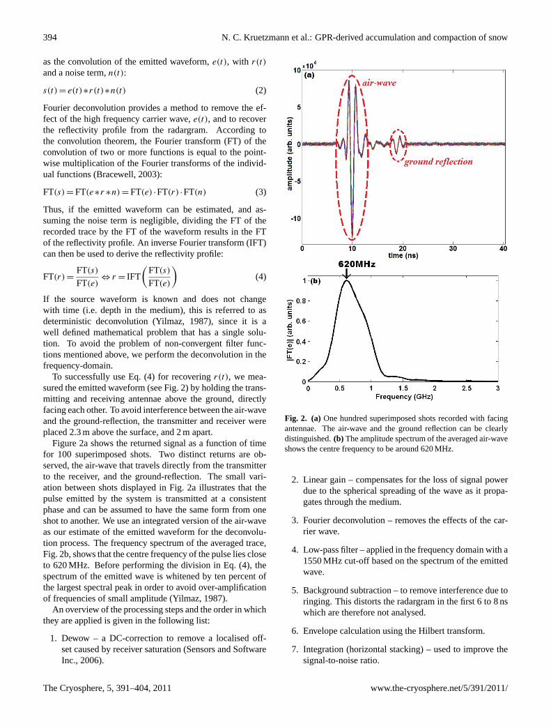
The decreasing trend in the depth of the dust horizon fromnorth to south observed at L2 (Fig. 7a) can be followed southalong a GPR transect (Fig. 9) that was recorded as an ex-tension of the line going from I1 to A1. Along this profile,

Fig. 8. Processed radargram from C1 to C9 at site L3 (2009). Thered box marks the approximate location of the firn core; the yellowarrow indicates the expected TWT to the dust layer.

the internal horizons gradually migrate upwards (not shown).After about 14 km, the horizon we associate with the dustlayer becomes too indistinct to be reliably identified. At thispoint, the dust layer reflection is found at a depth of about1.9 m, which is equivalent to a reduced average accumulationof approximately 165 kg m−2 a−1 (see Fig. 9). This has to beconsidered a crude estimate, since it assumes the same aver-age snow density between the surface and the dust layer asat L2. A qualitatively similar trend was previously reportedby both Heine (1967) and the McMurdo Ice Shelf Project(McCrae, 1984).

Unfortunately, we were unable to reliably date other layerswithin the snow pit or firn core profiles and associate themwith discrete reflections in the radargram. However, due tothe high precision of the system, the vertical separation ofother apparent horizons can be used to estimate compaction,which is the focus of the next section.

4.3 Snow compaction

Most of the apparent internal horizons found in the 2008GPR data can also be identified in the following year’srecords. Figure 6c shows nine reflections tracked betweenstakes E4 and E6 at L2 in 2008, and Fig. 6d shows the samehorizons tracked in the 2009 data. One might expect thatcompaction, caused by temperature metamorphosis and theadditional overburden on the surface, will reduce the sepa-ration between horizon pairs. This is confirmed by the pooralignment of the bottom horizon (IX) in Fig. 6d compared toFig. 6c. Clearly, the total separation between the top (I) andthe bottom (IX) reflection has been reduced. Assuming thatthe same horizons have been identified, calculating the aver-age separation between two successive horizons in 2008 andcomparing it with that of the same horizon pair in the 2009

The Cryosphere, 5, 391–404, 2011 www.the-cryosphere.net/5/391/2011/

N. C. Kruetzmann et al.: GPR-derived accumulation and compaction of snow 399

Fig. 9. Accumulation along a transect from L2 to L1, estimated bytracking the dust layer reflection for 14 km.

data, allows us to estimate the compaction of the snow in theintervening time period.

Not all horizons in Fig. 6c and d are suitable for com-paction calculations because the high variability of the un-dulating horizon, for example, does not allow it to be trackedreliably enough to be confident that the same horizon was se-lected in both years. Similarly, the relatively strong double-horizon visible between 41 ns and 46 ns in 2008 (Fig. 6a)and between 45 ns and 49 ns in 2009 (Fig. 6b) may be easyto recognise visually, but the noise between both horizonsmakes them unreliable for automated tracking. In order toestablish which of the reflections are likely to be reliablytracked in both years, we calculate the correlation betweenthe TWT profile of each horizon in 2008 and its counter-part in 2009. Additionally, we calculate the distance betweenpairs of horizons in terms of TWT for each year and the cor-relation of these relative TWT profiles. Only those horizonsthat show a correlation greater than 0.5 in all cases are usedfor compaction calculations. To ensure accuracy, we also re-quire a minimum average TWT difference between horizonsof 10 ns, corresponding to approximately 1 m vertical sepa-ration.

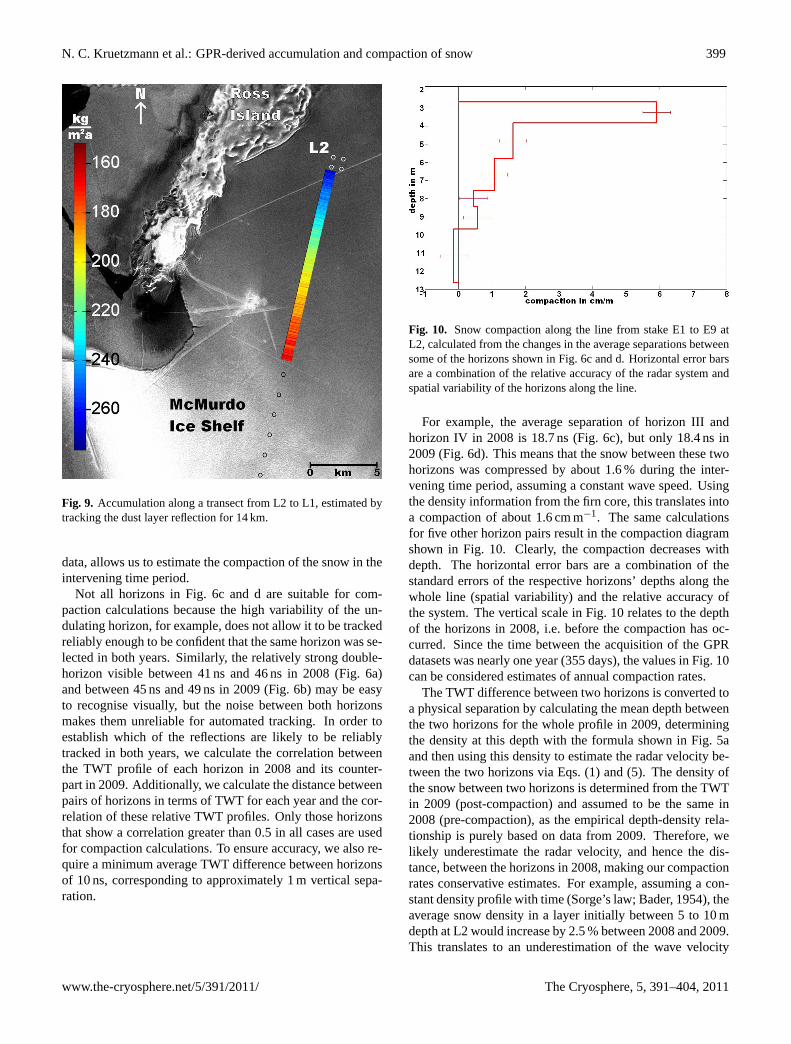
Fig. 10. Snow compaction along the line from stake E1 to E9 atL2, calculated from the changes in the average separations betweensome of the horizons shown in Fig. 6c and d. Horizontal error barsare a combination of the relative accuracy of the radar system andspatial variability of the horizons along the line.

For example, the average separation of horizon III andhorizon IV in 2008 is 18.7 ns (Fig. 6c), but only 18.4 ns in2009 (Fig. 6d). This means that the snow between these twohorizons was compressed by about 1.6 % during the inter-vening time period, assuming a constant wave speed. Usingthe density information from the firn core, this translates intoa compaction of about 1.6 cm m−1. The same calculationsfor five other horizon pairs result in the compaction diagramshown in Fig. 10. Clearly, the compaction decreases withdepth. The horizontal error bars are a combination of thestandard errors of the respective horizons’ depths along thewhole line (spatial variability) and the relative accuracy ofthe system. The vertical scale in Fig. 10 relates to the depthof the horizons in 2008, i.e. before the compaction has oc-curred. Since the time between the acquisition of the GPRdatasets was nearly one year (355 days), the values in Fig. 10can be considered estimates of annual compaction rates.

The TWT difference between two horizons is converted toa physical separation by calculating the mean depth betweenthe two horizons for the whole profile in 2009, determiningthe density at this depth with the formula shown in Fig. 5aand then using this density to estimate the radar velocity be-tween the two horizons via Eqs. (1) and (5). The density ofthe snow between two horizons is determined from the TWTin 2009 (post-compaction) and assumed to be the same in2008 (pre-compaction), as the empirical depth-density rela-tionship is purely based on data from 2009. Therefore, welikely underestimate the radar velocity, and hence the dis-tance, between the horizons in 2008, making our compactionrates conservative estimates. For example, assuming a con-stant density profile with time (Sorge’s law; Bader, 1954), theaverage snow density in a layer initially between 5 to 10 mdepth at L2 would increase by 2.5 % between 2008 and 2009.This translates to an underestimation of the wave velocity

www.the-cryosphere.net/5/391/2011/ The Cryosphere, 5, 391–404, 2011

400 N. C. Kruetzmann et al.: GPR-derived accumulation and compaction of snow

in 2008 by approximately 1 % and an increase in the com-paction rates of about 0.5 cm m−1.

The apparent expansion observed below 10 m in Fig. 10probably indicates the error in our measurements, and theactual amount of compaction over a one year time period atthis depth is too small to be measured with our system. Fur-thermore, below 8.4 m the conversion from TWT to depth isbased solely on an extrapolation of the exponential fit to thedensity data from the firn core, causing additional uncertain-ties in the calculations.

The same calculations were performed for five more linesat L2 (A2–I2, A5–I5, A7–I7, B1–B9, and H1–H9) and aresummarised in Fig. 11a. The vertical error bars indicate theaverage separation of the two horizons in 2008. Figure 11ashows that the variability in layer depths and compaction be-tween these six lines is small and thus tracking was not re-peated for the remaining lines. The thicker, black data pointspresent the average compaction between each of the horizonpairs and the connecting line illustrates the decreasing trend.

Figure 11b was calculated using the same methodology onseven internal horizons at L3. At this site, the variability ofthe compaction rates and the average depths is significantlyhigher. Therefore, the calculations were performed for allgrid lines, except for A9–I9 due to corrupt data. The largerspread is in accordance with the observed spatial variabil-ity in the accumulation pattern and the resulting dipping ofthe internal horizons (see Figs. 7b and 8). Nevertheless, themean compaction rate (black line) shows a clear trend of re-duced compaction with depth, similar to that observed at L2.

Assuming constant density profiles with time (Sorge’slaw) and using the measured average accumulation from thestake farms to determine the initial offsets, we can calcu-late expected compaction curves. The results are the dashedblue lines in Fig. 11a and b. In both cases the general trendmatches that of the compaction measurements, but aboveabout 4 m measured compaction rates are higher than thosepredicted by the model, and lower at greater depths.

5 Discussion

Table 1 summarises our results relating to accumulation. Atboth L2 and L3, the measurements derived from the stakefarms showed significantly less accumulation than the com-bined firn core and GPR measurements. This discrepancy isprobably largely due to temporal variability. If the readout ofthe stake depths had occurred one week later, the measure-ments at both sites would have been noticeably higher dueto the occurrence of a high precipitation event from the 13 to15 November 2009. The accumulation rates derived from thesnow pit and firn core observations should therefore be con-sidered more reliable, since they cover a longer time period.

The average accumulation at L2 – a site that is rel-atively typical for coastal areas – was found to be269± 9 kg m−2 a−1, which is much lower than the value re-ported by Heine (1967) at the closest station (510 kg m−2 a−1

Fig. 11. Snow compaction vs. depth for(a) L2 and (b) L3.(a) shows the compaction calculated from six lines at L2, while(b) includes all lines from L3 except one. The vertical axis repre-sents depth before compaction has occurred. The horizontal errorbars illustrate only the spatial variability along each of the lines,not measurement error. The vertical error bars show the thicknessof the layers before compaction. The thick black line representsthe average compaction for each horizon pair and the dashed blueline represents the expected compaction when assuming a constantdensity profile with time (Sorge’s law).

at station 200, about 6 km north east of our site). There is astrong accumulation gradient in this area and L2 is close tothe 320 kg m−2 a−1 contour suggested by McCrae (1984), avalue which still lies above our estimate.

Generally, the conversion of TWT to depth based on mea-sured densities is critical for our method and a potentialsource of error. A bias in the density data would lead toover- or under-estimation of the wave velocity in the snowand therefore the accumulation estimates, but good agree-ment between core- and snow pit densities from the two sea-sons at both sites (not shown) allows us to be confident inthe density measurements. As the dust layer is a reliable ref-erence point for dating, the difference between our resultsand previous studies could indicate an overall reduction inannual accumulation or high natural variability in this area.

The Cryosphere, 5, 391–404, 2011 www.the-cryosphere.net/5/391/2011/

N. C. Kruetzmann et al.: GPR-derived accumulation and compaction of snow 401

Moreover, historic accumulation rates derived from stakemeasurements are very likely to be underestimates, as theconsideration of snow compaction – as suggested by Taka-hashi and Kameda (2007) – is not reported.

The gradient in the accumulation map for L2 (Fig. 7a) isfound to continue along the transect toward L1 (Fig. 9). Thesouthernmost point up to which we were able to track thedust horizon lies relatively close to the location of a 20 m firncore analysed in Dunbar et al. (2009). They estimate an accu-mulation rate of 53± 20 cm of snow per year. If we assumean average density of 600 kg m−3 for the whole length oftheir core, this corresponds to 318± 120 kg m−2 a−1. Again,our estimate from the tracked reflection lies significantlylower at 165 kg m−2 a−1. However, the two points are ap-proximately 3 km apart and the conversion from TWT todepth uses the average column density down to the dust layerdetermined at L2, which is probably an underestimate for thislocation.

Only one reflection horizon could be associated with alayer in the snow stratigraphy acquired via simple glaciolog-ical tools and visual observation. Such difficulties in linkingsnow pit and radar observations are quite common (Harperand Bradford, 2003) and are due to the limited resolution ofour density profiles (Eisen et al., 2003). Furthermore, thestudy sites investigated here were located in areas of low di-electric variability. The snow was dry and homogeneous andtherefore contained few major dielectric contrasts, such asmight be caused by occasional melt layers (e.g., Dunse etal. 2008). Alley (1988) and Arcone et al. (2004) suggestthat a combination of thin layers and depth hoar are likelysources for GPR reflections in dry snow. While we did notobserve many distinct hoar layers in the snow pit and coredata, some may have been overlooked due to the coarsenessof the recorded density profile. Accurate identification of theorigin of the radar reflections would require high-resolutiondata from e.g. dielectric profiling, as suggested by Eisen etal. (2004) and Hawley et al. (2008).

The locations of the various horizons at the crossoverpoints of the grid are consistent between perpendicular pro-files. In most cases, the same reflection tracked along differ-ent profiles can be found within two time samples (2× 0.1 nswhich corresponds to 4 cm) at the point of intersection. Theconcurrence of the horizon depths is equally high for all re-flections at both L2 and L3, showing that the precision of theprocessed radar data is higher than the theoretical resolutionmight suggest. This high precision allowed us to estimatesnow compaction with depth from changes in the separationsof internal horizons from one year to the next.

At both L2 and L3, the average compaction measured be-tween 2 and 13 m depth over a one year time period rangesfrom 0 cm m−1 to 7 cm m−1. The sudden drop in compactionobserved below about 4 m at both sites (see Fig. 11) couldbe related to a change in the compaction mechanism. Freshsnow largely compacts via settling, but above a density of550 kg m−3 sintering is usually considered to become dom-

inant (Maeno, 1982; Van den Broeke, 2008). According tothe density profiles in Fig. 5, the 550 kg m−3 level lies around6 m depth at both sites, which compares well with the modelestimate by Van den Broeke (2008), who gives a range of 5 to8 m depth for the 550 kg m−3 level in this area. However, thedepth at which we observe a change in compaction rate (4 m)is more shallow than this theoretical threshold density. A re-cent study by Horhold et al. (2011) suggests that the “classic”picture of snow compaction is too simple, but better resolveddensity measurements would be required to explain the ori-gin of the observed step in compaction rate. Similarly, theorigin of the dip in compaction rate between 7.5 m and 8.5 mat L2 (Fig. 11a) could be a result of above average snow den-sity at this depth, possibly related to one or two particularlywarm summers, but we do not have sufficient data to testwhether this is a measurement error or a subsurface feature.

High resolution measurements of densification rates to di-rectly compare with our results are sparse. As we cannotidentify the 2008 surface in the radargrams from 2009, it isnot possible to calculate the total compaction of the wholesnow column. However, total compaction between 5 m and10 m depth can be estimated from Fig. 11 and compared tothe measurements from Arthern et al. (2010). Summing upthe average compaction (black lines in Fig. 11a and b) be-tween 5 m and 10 m, gives a total compaction of approxi-mately 4.3 cm at L2 (assuming zero compaction for the deep-est 30 cm, where the results are negative) and 5.5 cm at L3,over a time period of 355 days. Using the daily rates givenin Table 3 of Arthern et al. (2010) to calculate the total com-paction over the same time span and depth range gives 5.7 cmfor their “Berkner Island” site, the only site at which theirstrainmeters worked throughout the whole trial time. Whileour results qualitatively agree with the “Berkner Island” data,the other sites detailed in Arthern et al. (2010) show consid-erably higher compaction rates. As mentioned above, onereason for this could be that we do not take into account thechange in snow density due to compaction and its effect onthe velocity of the radar signal, since this would require ad-ditional density data for 2008. Ultimately, the discrepanciesbetween Arthern et al. (2010) and our results could also bedue to a difference in climatic conditions, since most of theirsites are located in regions with lower mean annual temper-ature, lower latitude, higher elevation and higher annual ac-cumulation. Therefore, considerable differences in the com-paction behaviour of the snow could be expected.

6 Summary and conclusion

The deterministic Fourier deconvolution scheme suggestedhere can be used to remove some of the effects of the car-rier signal from GPR data of dry firn, provided that it wasrecorded with a system that has a very stable output. Theresult is a more focussed radargram with improved con-trast. This type of processing improves the identificationand precise tracking of weak internal reflection horizons

www.the-cryosphere.net/5/391/2011/ The Cryosphere, 5, 391–404, 2011

402 N. C. Kruetzmann et al.: GPR-derived accumulation and compaction of snow

associated with density variations. The processing also fa-cilitates recognition of the same horizons in follow-up sur-veys. Our methodology also has the potential to work suc-cessfully for recordings in areas that are subject to sporadicmelt events, although one should keep in mind that an essen-tial assumption of the deconvolution is that there is no – oronly very little – frequency dependent absorption and disper-sion in the medium.

Using the thusly processed radargrams we extrapolatedpoint measurements of average accumulation from a snowpit at site L2 (251 kg m−2 a−1) and a firn core at site L3(437 kg m−2 a−1), to a larger area by identifying a dateabledust layer horizon in the radargram. From the GPR data theextrapolated average accumulation over the 800 m× 800 msite on the ice shelf in Windless Bight (L2) was found to be269± 9 kg m−2 a−1. The 400 m× 400 m grid on Ross Island(L3) showed higher variability in the internal horizons withan overall average accumulation of 404±22 kg m−2 a−1.Stake farm readings at both sites, maintained over approx-imately a one year time period, measured an accumulationof 224±21 kg m−2 a−1 at L2 and 304± 83 kg m−2 a−1 atL3. The discrepancy between these values and the combinedfirn core and GPR measurements was probably caused bythe short time period spanned by the stake observations andthe high temporal variability of precipitation events. Ad-ditionally, we measured a decreasing accumulation trendalong a 14 km long GPR transect heading south from L2.At the southernmost point, the accumulation was about165 kg m−2 a−1.

By comparing vertical separations of internal reflectionhorizons from one year to the next, we were able to estimatecompaction rates from GPR measurements down to 13 mdepth. This technique might have implications for the val-idation of the CryoSat-2 satellite altimeter which measuresthe surface height of ice sheets and shelves, in order to mon-itor the polar mass balance.

Our results show that internal reflectors found in GPRdata, combined with density information, can be used for es-timating compaction rates of dry snow. However, estimatingdensification in percolation areas is probably much more dif-ficult due to the more complex snow morphology (Parry etal., 2007). Frequent repetition of GPR measurements overa longer time period, combined with high resolution dielec-tric profiling of firn cores, could be used to establish a moredetailed representation of time-dependent firn densificationfor the validation of current firn densification models. Thesuggested method is applicable over large areas in an effi-cient and non-invasive manner and is complementary to pointmeasurements of snow compaction at a higher temporal res-olution, such as those performed by Arthern et al. (2010)and Heilig et al. (2010). Using a higher frequency system,it might also be possible to improve the vertical resolution ofsnow compaction data from GPR measurements.

Acknowledgements.The authors would like to thank StevenArcone and Olaf Eisen for their thorough reviews and suggestionsfor the improvement of the manuscript. This work was supportedby Antarctica New Zealand under the field event K053 “CryosphereRemote Sensing” and by scholarships from the Christchurch CityCouncil and the University of Canterbury for Nikolai Kruetzmann.The participation of Mette Riger-Kusk in the field work in 2008 isgreatly acknowledged. The measurements were conducted withinthe ESA CryoSat-2 calibration and validation activities for projectAOCRY2CAL-4512.

Edited by: M. Van den Broeke

References

Alley, R. B.: Concerning the deposition and diagenesis of strata inpolar firn, J. Glaciol., 34(118), 283–290, 1988.

Alley, R. B., Bolzan, J. F., and Whillans, I. M.: Polar firn densifica-tion and grain growth, Ann. Glaciol., 3, 7–11, 1982.

Arcone, S. A., Lawson, D., and Delaney, A.: Short-pulse waveletrecovery and resolution of dielectric contrasts within englacialand basal ice of Matanuska Glacier, Alaska, U.S.A., J. Glaciol.,41, 68–86, 1995.

Arcone, S. A., Spikes, V. B., Hamilton, G. S., and Mayewski, P. A.:Stratigraphic continuity in 400 MHz short-pulse radar profiles offirn in West Antarctica, Ann. Glaciol., 39, 195–200, 2004.

Arcone, S. A., Spikes, V. B., and Hamilton, G. S.: Stratigraphicvariation in polar firn caused by differential accumulation andice flow: Interpretation of a 400-MHz short-pulse radar profilefrom West Antarctica, J. Glaciol., 51(7), 407–422, 2005.

Arthern, R. J. and Wingham, D. J.: The natural fluctuations of firndensification and their effect on the geodetic determination of icesheet mass balance, Climatic Change, 40(4), 605–624., 1998.

Arthern, R. J., Vaughan, D. G., Rankin, A. M., Mulvaney, R., andThomas, E. R.: In situ measurements of Antarctic snow com-paction compared with predictions of models, J. Geophys. Res.,115, F03011,doi:10.1029/2009JF001306, 2010.

Bader, H.: Sorge’s law of densification of snow on high polarglaciers, J. Glaciol., 2(15), 319–323, 1954.

Bentley, C. R., Clough, J. W., Jezek, K. C., and Shabtaie, S.:Ice-thickness patterns and the dynamics of the Ross Ice Shelf,Antarctica, J. Glaciol., 24(90), 287–294, 1979.

Belina, F. A., Dafflon, B., Tronicke, J., and Holliger, K.: Enhancingthe vertical resolution of surface georadar data, J. Appl. Geo-phys., 68, 26–35,doi:10.1016/j.jappgeo.2008.08.011, 2009.

Bogorodsky, V. V., Bentley, C. R., and Gudmandsen, P. E.: Ra-dioglaciology, D. Reidel Publishing Company, Norwell, Mas-sachusetts, ISBN 90-277-1893-9, 1985.

Bracewell, R. N.: Fourier analysis and imaging, Kluwer Aca-demic/Plenum Publishers, New York, New York, ISBN 0-306-48187-1, 2003.

Davis, C. H. and Ferguson, A. C.: Elevation Change of the Antarc-tic Ice Sheet, 1995–2000, from ERS-2 Satellite Radar Altimetry,IEEE Trans. Geosci. Remote Sens., 42(11), 2437–2445, 2004.

Davis, C. H., Li, Y., McConnell, J. R., Frey, M. M., and Hanna, E.:Snowfall-Driven Growth in East Antarctic Ice Sheet MitigatesRecent Sea-Level Rise, Science, 308, 1898–1901, 2005.

The Cryosphere, 5, 391–404, 2011 www.the-cryosphere.net/5/391/2011/

N. C. Kruetzmann et al.: GPR-derived accumulation and compaction of snow 403

Drinkwater, M. R., Long, D. G., and Bingham, A. W.: Greenlandsnow accumulation estimates from satellite radar scatterometerdata, J. Geophys. Res., 106(D24), 33935–33950, 2001.

Dunbar, G. B., Bertler, N. A. N., and McKay, R. M.: Sed-iment flux through the McMurdo Ice Shelf in WindlessBight, Antarctica, Global and Planetary Change, 69, 87–93,doi:10.1016/j.gloplacha.2009.05.007, 2009.

Dunse, T., Eisen, O., Helm, V., Rack, W., Steinhage, D., and Parry,V.: Characteristics and small-scale variability of GPR signals andtheir relation to snow accumulation in Greenland’s percolationzone, J. Glaciol., 54(185), 333–342, 2008.

Eisen, O., Wilhelms, F., Nixdorf, U., and Miller, H.: Reveal-ing the nature of radar reflections in ice: DEP-based FDTDforward modeling, Geophys. Res. Lett., 30(5), 1218–1221,doi:10.1029/2002GL016403, 2003.

Eisen, O., Nixdorf, U., Wilhelms, F., and Miller, H.: Age estimatesof isochronous reflection horizons by combining ice core, survey,and synthetic radar data, J. Geophys. Res.-Sol. Ea., 109, B04106,doi:10.1029/2003JB002858, 2004.

Eisen, O., Frezzotti, M., Genthon, C., Isaksson, E., Magand, O.,Van den Broeke, M. R., Dixon, D. A., Ekaykin, A., Holm-lund, P., Kameda, T., Karlo, L., Kaspari, S., Lipenkov, V. Y.,Oerter, H., Takahashi, S., and Vaughan, D. G.: Ground-basedmeasurements of spatial and temporal variability of snow ac-cumulation in East Antarctica, Rev. Geophys., 46, RG2001,doi:10.1029/2006RG000218, 2008.

Harper, J. T. and Bradford, J. H.: Snow stratigraphy over a uni-form depositional surface: spatial variability and measurementtools, Cold Reg. Sci. Technol., 37, 289–298,doi:10.1016/S0165-232X(03)00071-5, 2003.

Hawley, R. L., Brandt, O., Morris, E. M., Kohler, J., Shepherd,A. P., and Wingham, D. J.: Techniques for measuring high-resolution firn density profiles: case study from Kongsvegen,Svalbard, J. Glaciol., 54(186), 463–468, 2008.

Heilig, A., Eisen, O., and Schneebeli, M.: Temporal observations ofa seasonal snowpack using upward-looking GPR, Hydrol. Pro-cess., 24, 3133–3145,doi:10.1002/hyp.7749, 2010.

Heine, A. J.: The McMurdo Ice Shelf Antarctica – A preliminaryreport, New Zeal. J. Geol. Geop., 10(2), 474–478, 1967.

Helm, V., Rack, W., Cullen, R., Nienow, P., Mair, D., Parry, V., andWingham, D. J.: Winter accumulation in the percolation zone ofGreenland measured by airborne radar altimeter, Geophys. Res.Lett., 34(6), L06501,doi:10.1029/2006GL029185, 2007.

Horhold, M. W., Kipfstuhl, S., Wilhelms, F., Freitag, J., and Fren-zel, A.: The densification of layered polar firn, J. Geophys. Res.,116, F01001,doi:10.1029/2009JF001630, 2011.

Irving, J. D. and Knight, R. J.: Removal of wavelet dispersionfrom ground-penetrating radar data, Geophysics, 68(3), 960–970,doi:10.1190/1.1581068, 2003.

Kovacs, A., Gow, A. J., and Morey, R. M.: The in-situ dielectricconstant of polar firn revisited, Cold Reg. Sci. Technol., 23, 245–256, 1995.

Maeno, N.: Densification rates of snow at polar glaciers, Memoirsof the National Institute of Polar Research, Special Issue, 24, 48–61, 1982.

McCrae, I. R.: A summary of glaciological measurements madebetween 1960 and 1984 on the McMurdo ice shelf, Antarctica:a report submitted to the Antarctic Division of D.S.I.R., Auck-land, Dept. of Theoretical and Applied Mechanics: University of

Auckland, 1984.Nguyen, A. T. and Herring, T. A.: Analysis of ICESat data using

Kalman filter and kriging to study height changes in East Antarc-tica, Geophys. Res. Lett., 32, L23S03, Memoirs of the NationalInstitute of Polar Researchdoi:10.1029/2005GL024272, 2005.

Parry, V., Nienow, P., Mair, D., Scott, J., Hubbard, B., Steffen, K.,and Wingham, D.: Investigations of meltwater refreezing anddensity variations in the snowpack and firn within the percolationzone of the Greenland ice sheet, Ann. Glaciol., 46, 61–68, 2007.

Rial, F. I., Henrique, L., Pereira, M., and Armesto, J.: Wave-form Analysis of UWB GPR Antennas, Sensors, 9, 1454–1470,doi:10.3390/s90301454, 2009.

Rotschky, G., Rack, W., Dierking, W., and Oerter, H.: RetrievingSnowpack Properties and Accumulation Estimates From a Com-bination of SAR and Scatterometer Measurements, IEEE Trans.Geosci. Remote Sens., 44(4), 943–956, 2006.

Sensors and Software Inc.: pulseEKKO PRO – User’s Guide, Mis-sissauga, Ontario, Canada, 2006.

Spikes, V. B., Hamilton, G. S., Arcone, S. A., Kaspari, S., andMayewski, P. A.: Variability in Accumulation Rates from GPRProfiling on the West Antarctic Plateau, Ann. Glaciol., 39, 238–244, 2004.

Steinhoff, D. F., Bromwich, D. H., Lambertson, M., Knuth, S. L.,Lazzara, M. A.: A Dynamical Investigation of the May 2004McMurdo Antarctica Severe Wind Event Using AMPS, MonthlyWeather Review, 136, 7–26,doi:10.1175/2007MWR1999.1,2008.

Taner, M. T., Koehler, F., and Sheriff, R. E.: Complex seismic traceanalysis, Geophysics, 44(6), 1041–1063, 1979.

Takahashi, S. and Kameda, T.: Snow density for measuring surfacemass balance using the stake method, J. Glaciol., 53(183), 677–680, 2007.

Turner, G.: Subsurface radar propagation deconvolution, Geo-physics, 59(2), 215–223, 1994.

Ulrych, T. J.: The whiteness hypothesis: Reflectivity, inversion,chaos, and Enders, Geophysics, 64, 1512–1523, 1999.

Van den Broeke, M.: Depth and Density of the Antarctic Firn Layer,Arct. Antarct. Alp. Res., 40(2), 432–438, 2008.

Walden, A. T. and Hosken, J. W. J.: An Investigation of theSpectral Properties of Primary Reflection Coefficients, Geophys.Prospect., 33, 400–435, 1985.

Wingham, D. J., Ridout, A. J., Scharroo, R., Arthern, R. J., andShum, C. K.: Antarctic Elevation Change from 1992 to 1996,Science, 282, 456–458, 1998.

Wingham, D. J., Francis, C. R., Baker, S., Bouzinac, C., Brockley,D., Cullen, R., de Chateau-Thierry, P., Laxon, S. W., Mallow, U.,Mavrocordatos, C., Phalippou, L., Ratier, G., Rey, L., Rostan, F.,Viau, P., and Wallis, D. W.: CryoSat: A mission to determinethe fluctuations in Earth’s land and marine ice fields, Adv. SpaceRes., 37, 841–871, 2006.

Xia, J., Franseen, E. K., Miller, R. D., Weis, T. V.: Application ofdeterministic deconvolution of ground-penetrating radar data in astudy of carbonate strata, J. Appl. Geophys., 56, 213–229, 2004.

Xiao, Q. N., Kuo, Y. H., Ma, Z. Z., Huang, W., Huang, X. Y., Zhang,X., Barker, D. M., Michalakes, J., and Dudhia, J.: Application ofan Adiabatic WRF Adjoint to the Investigation of the May 2004McMurdo, Antarctica, Severe Wind Event, Monthly WeatherReview, 136(10), 3696–3713,doi:10.1175/2008MWR2235.1,2008.

www.the-cryosphere.net/5/391/2011/ The Cryosphere, 5, 391–404, 2011

404 N. C. Kruetzmann et al.: GPR-derived accumulation and compaction of snow

Yilmaz, O.: Seismic Data Processing, Society of Exploration Geo-physicists, Tulsa, OK, USA, 1987.

Zwally, H. J. and Li, J.: Seasonal and interannual variations offirn densification and ice-sheet surface elevation at the Greenlandsummit, J. Glaciol., 48(161), 199–207, 2002.

The Cryosphere, 5, 391–404, 2011 www.the-cryosphere.net/5/391/2011/