sma206

December 22, 2009

SMA 206: INTRODUCTION TO ANALYSIS

Lecture Notes

First Edition

By

Dr. Bernard Mutuku Nzimbi, PhD

School of Mathematics, University of Nairobi

P.o Box 30197, Nairobi, KENYA.

Copyright c© 2009 Benz, Inc. All rights reserved.

Contents

Preface iv

Acknowledgements v

Dedication 1

1 THE REAL NUMBERS SYSTEM 2

1.1 Introduction . . . . . . . . . . . . . . . . . . . . . . . . . . . . . . . . . . 2

1.2 ALGEBRAIC AND ORDER PROPERTIES OF R . . . . . . . . . . . . 4

1.2.1 FIELD AXIOMS . . . . . . . . . . . . . . . . . . . . . . . . . . . 4

1.2.2 ORDER AXIOMS . . . . . . . . . . . . . . . . . . . . . . . . . . 6

1.3 OTHER PROPERTIES OF R AND ITS SUBSETS . . . . . . . . . . . . 11

1.3.1 Properties of Integers . . . . . . . . . . . . . . . . . . . . . . . . . 11

1.3.2 Properties of Rationals and Irrationals . . . . . . . . . . . . . . . 11

1.3.3 Properties of the Positive Real Numbers . . . . . . . . . . . . . . 13

2 THE UNCOUNTABILITY OF R 23

2.1 Introduction . . . . . . . . . . . . . . . . . . . . . . . . . . . . . . . . . . 23

2.2 COUNTABLE SETS . . . . . . . . . . . . . . . . . . . . . . . . . . . . . 24

2.3 THE UNCOUNTABILITY OF R . . . . . . . . . . . . . . . . . . . . . . 30

2.3.1 INTERVALS ON THE REAL LINE . . . . . . . . . . . . . . . . 31

2.3.2 Nested Intervals . . . . . . . . . . . . . . . . . . . . . . . . . . . . 32

2.3.3 Nested Interval Property . . . . . . . . . . . . . . . . . . . . . . . 32

i

3 STRUCTURE OF THE METRIC SPACE R 39

3.1 Introduction . . . . . . . . . . . . . . . . . . . . . . . . . . . . . . . . . . 39

3.2 The notion of a metric . . . . . . . . . . . . . . . . . . . . . . . . . . . . 40

3.2.1 Examples of Metrics . . . . . . . . . . . . . . . . . . . . . . . . . 40

3.3 Neighbourhoods, Interior points and Open sets . . . . . . . . . . . . . . . 42

3.3.1 Neighborhoods in a metric space . . . . . . . . . . . . . . . . . . 42

3.4 Limit Points and Closed sets . . . . . . . . . . . . . . . . . . . . . . . . . 46

3.5 Properties of open and closed sets in R . . . . . . . . . . . . . . . . . . . 49

3.6 Relatively Open and Closed Sets . . . . . . . . . . . . . . . . . . . . . . 50

3.7 Solved Problems . . . . . . . . . . . . . . . . . . . . . . . . . . . . . . . 51

3.8 Tutorial Problems . . . . . . . . . . . . . . . . . . . . . . . . . . . . . . . 53

4 BOUNDED SUBSETS OF R 55

4.1 Introduction . . . . . . . . . . . . . . . . . . . . . . . . . . . . . . . . . . 55

4.2 Upper Bounds, Lower Bounds of a subset of R . . . . . . . . . . . . . . . 55

4.2.1 Supremum and Infimum of a subset of R . . . . . . . . . . . . . . 56

4.3 The Completeness Property of R . . . . . . . . . . . . . . . . . . . . . . 59

4.4 Solved Problems . . . . . . . . . . . . . . . . . . . . . . . . . . . . . . . 60

5 SEQUENCES OF REAL NUMBERS 63

5.1 Introduction . . . . . . . . . . . . . . . . . . . . . . . . . . . . . . . . . . 63

5.2 Convergence of a sequence . . . . . . . . . . . . . . . . . . . . . . . . . . 64

5.2.1 Criterion of Convergence . . . . . . . . . . . . . . . . . . . . . . . 64

5.2.2 Bounded Sequences . . . . . . . . . . . . . . . . . . . . . . . . . 68

5.3 Subsequences and the Bolzano-Weierstrass Theorem . . . . . . . . . . . . 69

5.4 Monotonic Sequences . . . . . . . . . . . . . . . . . . . . . . . . . . . . . 72

5.5 Limit Superior and Limit Inferior of a sequence . . . . . . . . . . . . . . 73

5.6 Cauchy Sequences . . . . . . . . . . . . . . . . . . . . . . . . . . . . . . . 76

5.7 Solved Problems . . . . . . . . . . . . . . . . . . . . . . . . . . . . . . . 78

6 LIMITS AND CONTINUITY OF FUNCTIONS IN R 80

6.1 Introduction . . . . . . . . . . . . . . . . . . . . . . . . . . . . . . . . . . 80

6.2 Limit of a Function . . . . . . . . . . . . . . . . . . . . . . . . . . . . . . 80

ii

6.3 Some results on Limits of Real-valued Functions . . . . . . . . . . . . . . 83

6.3.1 Limit Theorems . . . . . . . . . . . . . . . . . . . . . . . . . . . . 83

6.3.2 Limits at Infinity . . . . . . . . . . . . . . . . . . . . . . . . . . . 84

6.4 Continuous Functions in R . . . . . . . . . . . . . . . . . . . . . . . . . . 85

6.5 Uniform Continuity . . . . . . . . . . . . . . . . . . . . . . . . . . . . . . 89

6.6 Points of Discontinuity of a Function . . . . . . . . . . . . . . . . . . . . 91

6.6.1 Right and Left Limits . . . . . . . . . . . . . . . . . . . . . . . . 91

6.6.2 Types of Discontinuities . . . . . . . . . . . . . . . . . . . . . . . 92

6.7 Solved Problems . . . . . . . . . . . . . . . . . . . . . . . . . . . . . . . 96

7 PROPERTIES OF CONTINUOUS FUNCTIONS IN R 101

7.1 Introduction . . . . . . . . . . . . . . . . . . . . . . . . . . . . . . . . . . 101

7.2 Boundedness Theorem . . . . . . . . . . . . . . . . . . . . . . . . . . . . 102

7.3 Location of Roots Theorem . . . . . . . . . . . . . . . . . . . . . . . . . 102

7.4 Bolzano’s Intermediate Value Theorem (IVT) . . . . . . . . . . . . . . . 103

7.4.1 Applications of the IVT ( Existence and location of real roots of

polynomial equations) . . . . . . . . . . . . . . . . . . . . . . . . 105

7.5 Solved Problems . . . . . . . . . . . . . . . . . . . . . . . . . . . . . . . 106

8 THE RIEMANN INTEGRAL 108

8.1 Introduction . . . . . . . . . . . . . . . . . . . . . . . . . . . . . . . . . . 108

8.2 Partitions of an Interval . . . . . . . . . . . . . . . . . . . . . . . . . . . 108

8.3 Lower and Upper Riemann Sums . . . . . . . . . . . . . . . . . . . . . . 112

8.4 Upper and Lower Riemann Integrals . . . . . . . . . . . . . . . . . . . . 114

8.5 The Riemann Integral . . . . . . . . . . . . . . . . . . . . . . . . . . . . 115

8.5.1 Criterion for Riemann Integrability . . . . . . . . . . . . . . . . . 116

8.5.2 Some Classes of Riemann Integrable Functions . . . . . . . . . . . 118

8.6 Integral as a Limit . . . . . . . . . . . . . . . . . . . . . . . . . . . . . . 122

8.7 Solved Problems . . . . . . . . . . . . . . . . . . . . . . . . . . . . . . . 125

Bibliography 128

iii

Preface

The study of mathematical analysis is indispensable for a prospective student of pure or

applied mathematics. It has great value for any undergraduate student who wishes to

go beyond the routine manipulations of formulas to solve standard problems, because

it develops the ability to think deductively, analyze mathematical situations, and ex-

tend ideas to a new context. The subject of analysis is one of the fundamental areas of

mathematics, and is the foundation for the study of many advanced topics, not only in

mathematics, but also in engineering and the physical sciences. A thorough understand-

ing of the concepts of analysis has also become increasingly important for the study

of advanced topics in economics and the social sciences. Topics such as Fourier series,

measure theory and integration are fundamental in mathematics and physics as well as

engineering, economics, and many other areas.

The only absolute prerequisites for mastering the material in the book are an interest

in mathematics and a willingness occasionally to suspend disbelief when a familiar idea

occurs in an unfamiliar guise. But only an exceptional student would profit from reading

the book unless he/she has previously acquired a fair working knowledge of the processes

of elementary calculus.

This book is a development of various courses designed for second year students of math-

ematics, humanities and third year students of education at the University of Nairobi,

whose preparation has been several courses in calculus and analytical geometry.

iv

Acknowledgements

v

Dedication

1

Chapter 1

THE REAL NUMBERS SYSTEM

1.1 Introduction

We discuss the essential properties of the real number system R. We exhibit a list of

fundamental properties associated with R and show how further properties can be de-

duced from them. We begin this chapter by studying the decomposition of the real line

into the following subsets:

1.1 The Natural Numbers, N

N = 1, 2, 3, ....This set is also called the set of counting numbers.

Definition 1.1 A non-empty set X is said to be closed with respect to a binary operation

∗ if for all a, b ∈ X, we have a ∗ b ∈ X.

Note that N is closed with respect to the usual addition and usual multiplication but

ont usual subtraction.

2

1.2 The Whole Numbers, WW = 0, 1, 2, 3, .... Note that W = 0 ∪ N.

Note that W is closed with respect to usual addition and multiplication but not under

subtraction.

1.3 The Integers, ZZ = ...,−3,−2,−1, 0, 1, 2, 3, .... Note that Z = −N ∪W.

This system guarantees solutions to every equation x + n = m with n,m ∈W. Clearly,

Z consists of numbers x such that x ∈ N or x = 0 or −x ∈ N. Z is closed w.r.t + and

×.

Note also that N ⊂W ⊂ Z.

1.4 The Rational Numbers, QA rational number r is one that can be expressed in the form r = a

b, for a, b ∈ Z, b 6= 0

and (a, b) = 1, where (a, b) denotes the greatest common divisor of a and b.

Definition 1.2 The set of rationals, denoted by Q, is given by

Q = ab

: a, b ∈ Z, b 6= 0, (a, b) = 1.

With this system, solutions to all equations nx + m = 0 with m,n ∈ Z, and n 6= 0 can

be uniquely found: i.e. x = −n−1m = −mn.

Examples: 2, 0, 12, − 5

900.

Note that N ⊂W ⊂ Z ⊂ Q.

3

1.5 The Irrational Numbers, QC

An irrational number s is one that is not rational, i.e. s cannot be expressed as

s = ab, a, b ∈ Z, b 6= 0 and (a, b) = 1.Note that the sets of rationals and irrationals are

complements of each other.

Examples:√

2,√

3, Π.

Remark:√

p , where p is a prime number is always an irrational number. This

result will be proved towards the end of this chapter.

1.6 The Real Numbers, RThe set of reals is the union of the set of rationals with the set of irrationals, i.e.

R = Q⋃QC . Graphically, R is represented by the real number line and called the real

number system.

1.2 ALGEBRAIC AND ORDER PROPERTIES OF R

We now introduce the ”algebraic” properties, often called the ”field” axioms that are

based on the two binary operations of addition and multiplication.

We start with a given set S whose elements will be called numbers and consider the

following axioms for this set:

1.2.1 FIELD AXIOMS

(I) Addition Axioms: There is an addition operation ”+” such that for all numbers

x, y, z ∈ S the following hold:

1. x + y = y + x [ Commutativity ]

2. x + (y + z) = (x + y) + z [ Associativity ]

3. There is a number 0 such that x + 0 = x [ Existence of zero ]

4. For each x ∈ S there exists a number denoted −x such that

4

x + (−x) = 0; one writes y − x = y + (−x). [ Existence of Additive inverse]

(II) Multiplication Axioms: There is a multiplication operation ”.” such that for all

x, y, z ∈ S:

5. x.y = y.x [Commutativity]

6. x.(y.z) = (x.y).z [Associativity]

7. There is a number 1 such that 1.x = x [Existence of unity or unit element]

8. For each x 6= 0, ∃ a number x−1 such that x.x−1 = 1; one writes y.x−1 = yx. [

Existence of Reciprocals ]

9. x.(y + z) = x.y + x.z [ Distributivity ]

10. 1 6= 0 [ Non-triviality ]

Any set or ”number system” with operations + and . obeying these rules is called a field.

For example, the rational numbers, Q, the reals, R are fields. The set of integers, Z is

not a field since the reciprocal of an integer (other than ±1) is not an integer.

The identities 0 and 1 are defined in W. Addition and multiplication are also defined in

W. However, the Existence of additive inverse and the Existence of reciprocals axioms

do not hold in W.

Axiom 10 outlaws the trivial field consisting of the single element 0.

Axioms 1 and 2 hold along with 5, 6, 7, 9, and 10 in N.

Z obeys axioms 1 through 7, 9, and 10.

Q and R obey all these axioms.

From the field axioms, one can deduce the usual properties for manipulation of alge-

braic equalities, such as deriving the identity (a − b)2 = a2 − 2ab + b2 and the laws of

exponents.

The real numbers also come equipped with a natural ordering. We usually visualize

them arranged on a line.

5

1.2.2 ORDER AXIOMS

(III) There is a relation ”≤” such that

11. For each x we have x ≤ x. [Reflexivity]

12. If x ≤ y and y ≤ x, then x = y. [Antisymmetry]

13. If x ≤ y and y ≤ z, then x ≤ z. [Transitivity]

14. For every pair of numbers (x, y), either x ≤ y or y ≤ x. [Linear ordering]

15. If x ≤ y then x + z ≤ y + z for every z. [Compatibility of ≤ and +].

16. If 0 ≤ x and 0 ≤ y then 0 ≤ xy. [Compatibility of ≤ and .]

Remark

Properties 11 and 13 state that the relation ”≤” is a partial ordering. Property 14 says

that every two numbers are comparable. This is described by saying that ≤ is a linear

ordering or a total ordering.

Definition 1.3 A system obeying all 16 properties listed above is called an ordered field.

Examples: Q and R are ordered fields.

W is well-ordered by ≤.

Remark: By definition, x < y shall mean that x ≤ y and x 6= y.

The ”order properties” of R refer to the notions of positivity and inequalities between

real numbers. Properties 11, 12 and 14 combine to give the following observation:

The Law of Trichotomy

If x and y are elements of an ordered field, then exactly one of the relations

x < y, x = y or x > y holds.

Remark:

6

There are other systems besides real numbers in which some of these axioms play a role.

For example, axioms 1 through 9 excluding 5 and 8 define a ring. Axioms 1 through 4

define a commutative group.

We use some of the axioms to prove the following result:

Proposition 1.1 . In an ordered field the following properties hold:

(i). Unique identities:

If a + x = a for every a, then x = 0.

If a.x = a for every a, then x = 1.

(ii). Unique inverses:

If a + x = 0, then x = −a.

If ax = 1, then x = a−1.

(iii). No divisors of zero:

If xy = 0, then x = 0 or y = 0.

(iv). Cancellation Laws for addition:

If a + x = b + x, then a = b.

If a + x ≤ b + x ≤, then a ≤ b.

(v). Cancellation Laws for multiplication:

If ax = bx and x 6= 0, then a = b.

If ax ≥ bx and x > 0, then a ≥ b.

7

(vi). 0.x = 0 for every x.

(vii). −(−x) = x for every x.

(viii).−x = (−1)x for every x.

(ix). If x 6= 0, then x−1 6= 0 and (x−1)−1 = x.

(x). If x 6= 0 and y.= 0, then xy 6= 0 and (xy)−1 = x−1y−1.

(xi). If x ≤ y and 0 ≤ z, then xz ≤ yz.

If x ≤ y and z ≤ 0, then yz ≤ xz.

(xii). If x ≤ 0 and y ≤ 0, then xy ≥ 0.

If x < 0 and y ≥ 0, then xy ≤ 0.

(xiii). 0 < 1.

(xiv). For any x, x2 ≥ 0.

Proof

(i). Suppose x + a = a. Then

x = x + 0 = x + (a + (−a)) = (x + a) + (−a) = a + (−a) = a + (−1)a = (1 + (−1))a =

0.a = 0.

Likewise, suppose ax = a for all a. Then

x = x.1 = x(a.a−1) = (a.x)a−1 = a.a−1 = 1.

(ii). Suppose a + x = 0. Then

8

−a = −a + 0 = −a + (a + x) = (−a + a) + x = 0 + x = x, and so −a = x, as desired.

Likewise, if ax = 1, then a−1 = a−1.1 = a−1(ax) = (a−1a)x = 1.x = x.

(iii). It suffices to assume that x 6= 0 and prove that y = 0. Multiply xy by 1x

and apply

Associativity of multiplication, Existence of reciprocals, and Existence of unit axioms

to get:

1x(x.y) = (( 1

x).x).y = 1.y = y. Since xy = 0, ( 1

x)(xy) = 1

x.0 = 0. Thus y = 0.

(iv). Suppose a + x = b + x. Then

a = a + 0 = a + (−x + x) = −x + (a + x) = −x + (b + x) = (−x + x) + b = 0 + b = b.

Likewise, suppose a + x ≤ b + x. Then (a + x) + (−)(b + x) ≤ 0. That is, (a− b) + (x +

(−x)) ≤ 0, i.e. (a− b) + 0 ≤ 0, i.e. (a− b) ≤ 0. Adding b both sides, we have a ≤ b.

(v). Suppose that ax = bx and x 6= 0. Then ax +−(bx) = 0. That is, (a + (−b))x = 0.

Since x 6= 0, x−1 exists and (a + (−b))x.x−1 = 0.x−1 = 0. That is, a + (−b) = 0 i.e.

a = b.

Likewise, suppose that ax ≥ bx and x > 0. Then ax− bx ≥ 0. That is, (a+(−b))x ≥ 0.

Since x > 0 ⇒(a-b)≥ 0 ⇒a≥ b.

(vi). 0.x = (0 + 0)x = 0.x + 0.x, and so 0 = 0.x + (−0.x) = (0.x + 0.x) + (−0.x) =

0.x + (0.x + (−0.x)) = 0.x + 0.x = 0.x.

(viii). x + (−1)x = 1.x + (−1)x = (1 + (−1))x = 0.x = 0 by (vi). Thus, (−1).x = −x

by (ii).

(x). Suppose x 6= 0, y 6= 0 but xy = 0. Then since 0x = 0 by (vi), we have that

1 = ( 1y)( 1

x).xy = ( 1

y)( 1

x)0 = 0, contradiction to Proposition 1.1.1 axiom 10. Hence,

xy 6= 0. The proof of (xy)−1 = x−1y−1 is left as an exercise.

(xiii). Suppose 1 ≤ 0. Then 1 + (−1) ≤ 0 + (−1) and so 0 ≤ −1. Using property 16:

since 0 ≤ −1 and 0 ≤ −1, we get 0 ≤ (−1)(−1) = −(−1) = 1. Therefore, 1 ≤ 0 and

9

0 ≤ 1 and so 1 = 0 by property 12, in contradiction to property 10. Hence 0 < 1.

(xiv). Consider two cases: If x ≥ 0, then x2 = x.x ≥ 0, by axiom 16. If x < 0,

then x2 = (−(−x))(−(−x)) = (−1)2(−x)2, by (vii) and (viii). But (−1)2 = 1, since

0 = (−1)(−1 + 1) = (−1)2 + (−1).1 = (−1)2 − 1. Thus, x2 ≥ 0. ♣

Remark: The purposes of the axioms of an ordered field is to isolate the key properties

we need for manipulation of algebraic equalities and inequalities.

Example 1 Using the axioms and properties of an ordered field given in this section,

prove that a2 − b2 = (a− b)(a + b).

Solution

By the distributive law, (a− b)(a + b) = (a− b).a + (a− b).b. Using the commutativity

and the distributive law again, along with a− b = a + (−b):

(a− b).a + (a− b).b = a.(a− b) + b.(a− b) = a2 + a.(−b) + b.a + b.(−b).

Now,

a.(−b) = a.(−1).b = (−1)ab = −(ab) by Proposition 1.1.1 (viii), associativity and com-

mutativity. Similarly, b.(−b) = −b2. Thus, (a−b)(a+b) equals a2−a.(−b)+b.a+b.(−b) =

a2 − (ab) + ba− b2 = a2 − ab + ab− b2 ( by axiom 5)

= a2 − b2 (by axioms 3 and 4). ♣

Example 2 In an ordered field prove that if 0 ≤ x < y, then x2 ≤ y2.

Solution If 0 ≤ x < y, then 0 ≤ x ≤ y, and so by Proposition 1.1 (xi), x2 ≤ yx. By the

same reasoning, x ≤ y⇒xy≤ y2. Thus

x2 ≤ yx = xy ≤ y2, and so x2 ≤ y2. We now need to exclude the possibility that x2

equals y2. But if x2 = y2, then x2 − y2 = 0 (add −y2 to each side).

(x− y)(x + y) = 0 (by Example 1).

By Proposition 1.1(xii), we have 0 ≤ x and y > 0. Now x+ y 6= 0, since x+ y = 0 would

imply that y = (−x) ≤ 0, so that y ≤ 0, which is impossible by the Law of Trichotomy.

By the Cancelation Law for multiplication, (x− y)(x+ y) = 0, i.e. x− y = 0, i.e. x = y.

10

But we are given x < y, and so this case is excluded as desired. ♣

1.3 OTHER PROPERTIES OF R AND ITS SUBSETS

1.3.1 Properties of Integers

Definition 1.4 Let m ∈ Z. Then m is said to be even if it can be expressed as m = 2n,

for some n ∈ Z.

Definition 1.5 Let m ∈ Z. Then m is said to be odd if m = 2n + 1, for some n ∈ Z.

Proposition 1.2 (i). Let m ∈ Z. Then m is even iff m2 is even.

(ii). Let m ∈ Z. Then n is odd iff m2 is odd.

Proof

(i). (⇒) Let m ∈ Z be even. Then m = 2n for some n ∈ Z ⇒m2 = 4n2 = 2(2n2).

Hence m2 is divisible by 2, hence m2 is even.

(⇐) Conversely, let m2 be even and assume to the contrary that m is odd. Then

m = 2n + 1 for some n ∈ Z.

Therefore, m2 = (2n + 1)2 = 4n2 + 4n + 1 = 2(2n2 + 2n) + 1, where 2n2 + 2n ∈ Z. Thus

m2 is odd. This contradicts the fact that m2 is even.

Therefore, m must be even whenever m2 is even.

(ii). (⇒) Suppose m is odd. Then m = 2n + 1, for some n ∈ Z. So, m2 = (2n + 1)2 =

4n2 + 4n + 1 = 2(2n2 + 2n) + 1, where 2n2 + 2n ∈ Z. Hence m2 is odd.

(⇐) Conversely, let m2 be odd and assume to the contrary that m is even. Then m = 2n,

for some n ∈ Z. Therefore, m2 = 4n2 = 2(2n2), where 2n2 ∈ Z. Thus m2 is even, a

contradiction to our hypothesis that m2 is odd. Therefore m must be odd whenever m2

is odd. ♣

1.3.2 Properties of Rationals and Irrationals

Proposition 1.3 : Q is ”dense” in itself: If x and y are in Q, with x < y, then there

exists an element z ∈ Q such that x < z < y.

11

Proof

Choose z = x+y2

. ♣

Theorem 1.4 [Archimedian Property of R] If x, y ∈ R and x > 0, y > 0 and

x < y, then there exists a positive integer n such that nx > y.

Theorem 1.5 The Density Theorem If x and y are any real numbers with x < y,

then there exists a rational number r ∈ Q such that x < r < y.

Proof

Without loss of generality (WLOG) assume that x > 0. Since y − x > 0, ∃n ∈ N such

that 1n

< y − x. Therefore we have nx + 1 < ny. Since x > 0, we have nx > 0, there

exists m ∈ N with m−1 ≤ nx < m. Therefore, m ≤ nx+1 < ny, whence nx < m < ny.

Thus, the rational number r = mn

satisfies x < r < y. ♣

Proposition 1.6 QC is dense in R: If x and y are real numbers with x < y, then there

exists an irrational number z such that x < z < y.

Proof

Applying the Density Theorem to the real numbers x√2

and y√2, we obtain a rational

number r 6= 0 such that x√2

< r < y√2. If we let z = r

√2, then clearly z is irrational and

satisfies x < z < y. ♣

Remark:

If we start to mark the rational numbers on the number line, we find that they are

scattered densely along the line and seem to be filling it up. However, we know they

do not; for example√

2 is missing. That is, there exist at least one irrational real

number, namely√

2. There are ”more” irrational numbers than rational numbers in the

sense that the set of rational numbers is countable, while the set of irrational numbers

is uncountable. Concepts of countability and uncountability of sets will be studied in

Chapter 2.

This forms the basis of the following proposition:

Proposition 1.7√

2 is irrational.

12

Proof

We need to show that there does not exist an r ∈ Q such that r2 = 2.

We prove by contradiction. Assume to the contrary that√

2 is rational. Then by

definition,√2 = a

b, a, b ∈ Z, b 6= 0, (a, b) = 1.

(*)

Squaring both sides of (*), we have

2 = a2

b2or a2 = 2b2.

Therefore a2 is even, and hence a is even (by Proposition 1.2). Since a is even, a = 2k,

for some k ∈ Z. Hence, a2 = 4k2. But a2 = 2b2 = 4k2. That is b2 = 2k2 ⇒ b2 is even

and hence b is even (by Proposition 1.2). This means that 2 is a common factor for a

and b, a contradiction since (a, b) = 1 was our assumption. Hence√

2 is irrational. ♣

Proposition 1.8√

3 is irrational.

Proof

Assume to the contrary that√

3 is rational. Then√

3 = pq, with p, q ∈ Z, q 6= 0 and

(p, q) = 1. Therefore, 3 = p2

q2 or p2 = 3q2 which implies that 3 divides p2 and hence will

divide p (by Proposition 1.2). That is, p = 3k, for some k ∈ Z. Therefore, p2 = 9k2. But

p2 = 3q2, which implies that 3q2 = 9k2 or q2 = 3k2. Thus 3 divides q2 and hence q (by

Proposition 1.2). Thus m and n have a common factor 3. This leads to a contradiction

of our assumption. Hence,√

3 is irrational. ♣

Exercise. Prove that the√

p is irrational for any prime number p.

(Hint: Use a similar proof as above).

1.3.3 Properties of the Positive Real Numbers

We now define a nonempty subset P of R called the set of positive real numbers (some-

times denoted R+) that satisfies the following properties:

(i). If a, b ∈ P, then a + b ∈ P.

13

(ii). If a, b ∈ P, then ab ∈ P.

(iii). If a ∈ R , then exactly one of the following holds:

a ∈ P, a = 0, − a ∈ P [Trichotomy Property]

Remark

Property (iii) is the Trichotomy Property because it divides R into three distinct types

of elements. It states that the set −a : a ∈ P of negative real numbers has no elements

in common with the set P of positive real numbers, and , moreover, the set R is the

union of three disjoint sets.

Definition 1.6 If a ∈ P, we write a > 0 and say that a is a positive (or a strictly

positive) real number.

If a ∈ P ∪ 0, we write a ≥ 0 and say that a is a nonnegative real number. Similarly,

if −a ∈ P, we write a < 0 and say that a is negative (or strictly negative) real number.

If − a ∈ P ∪ 0, we write a ≤ 0 and say that a is a nonpositive real number.

Remark We now use the above definitions to prove the following theorem:

Theorem 1.9 Let a, b ∈ R.

(a). If a > b and b > c, then a > c.

(b). If a > b then a + c > b + c.

(c). If a > b and c > 0 , then ca > cb. If a > b and c < 0, then ca < cb.

Proof

(a). If a− b ∈ P and b− c ∈ P, then by the order properties of a field, this implies that

(a− b) + (b− c) = a− c belongs to P. Hence a > c.

(b). If a− b ∈ P, then (a + c)− (b + c) = a− b is in P. Thus a + c > b + c.

14

(c). If a− b ∈ P and c ∈ P, then ca− cb = c(a− b) is in P. Thus ca > cb when c > 0.

On the other hand, if c < 0, then −c ∈ P, so that cb− ca = (−c)(a− b) is in P. Thus

cb > ca when c < 0. ♣

Theorem 1.10 (a). If a ∈ R and a 6= 0, then a2 > 0.

(b). 1 > 0

(c). If n ∈ N, then n > 0.

Proof

(a). By the Trichotomy Property, if a 6= 0, then either a ∈ P or −a ∈ P. If a ∈ P, then

by the order property 3.(ii), a2 = a.a ∈ P. Also, if − a ∈ P, then a2 = (−a)(−a) ∈ P.

We conclude that if a 6= 0, then a2 > 0.

(b). Since 1 = 12, it follows from (a)that 1 > 0.

(c). We use Mathematical Induction: The assertion for n = 1 is true by (b). If we

suppose the assertion is true for the natural number k, then k ∈ P, and since 1 ∈ P,we

have k + 1 ∈ P by order property (i). Therefore, the assertion is true for all natural

numbers. ♣Remark

Theproductoftwopositivenumbersispositive.However, thepositivityofaproductoftwonumbersdoesnotimplythateachfactorispositive.

Theorem 1.11 If ab > 0, then either

(i). a > 0 and b > 0, or

(ii). a < 0 and b < 0.

Proof

Note that ab > 0 implies that a 6= 0 and b 6= 0. From the Trichotomy Property, either

a > 0 or a < 0. If a > 0, then 1a

> 0, and therefore b = ( 1a)(ab) > 0. Similarly, if

a < 0, then 1a

< 0, so that b = ( 1a)(ab) < 0. ♣

Corollary 1.12 If ab < 0, then either

15

(i). a < 0 and b > 0 or

(ii). a > 0 and b < 0.

We apply the above results in working with inequalities.

Inequalities

The order properties can be used to ”solve” certain inequalities.

Examples

(a). Determine the set A of all numbers x such that 2x + 3 ≤ 6.

Solution

x ∈ A iff 2x + 3 ≤ 5 iff 2x ≤ 3 iff x ≤ 3. Therefore A = x ∈ R : x ≤ 32.

(b). Determine the set B = x ∈ R : x2 + x > 2

Solution

Note that x ∈ B ⇔ x2 + x− 2 > 0 ⇔ (x− 1)(x + 2) > 0. Therefore, we either have

(i). x− 1 > 0 and x + 2 > 0 or we have

(ii). x− 1 < 0 and x + 2 < 0.

In case (i), we must have both x > 1 and x > −2, which is satisfied iff x > 1. In case

(ii), we must have both x < 1 and x < −2, which is satisfied iff x < −2. We conclude

that B = x ∈ R : x > 1 ∪ x ∈ R : x < −2.

(c). Determine the set C = x ∈ R : 2x+1x+2

< 1.

Note that C = x ∈ R : 2x+1x+2

− 1 < 0 = x ∈ R : 2x+1−(x+2)x+2

< 0 =

x ∈ R : x−1x+2

< 0

16

Therefore, we have either

(i). x− 1 < 0 and x + 2 > 0 or

(ii). x− 1 > 0 and x + 2 < 0.

In case (i), we must have both x < 1 and x > −2, which is satisfied iff −2 < x < 1. In

case (ii), we must have both x > 1 and x < −2, which is never satisfied. We conclude

that C = x ∈ R : −2 < x < 1.

Exercise

1. Let a ≥ 0 and b ≥ 0. Prove that a < b ⇔ a2 < b2 ⇔ √a <

√b.

Definition 1.7 If a and b are positive real numbers, then their arithmetic mean is12(a + b) and their geometric mean is

√ab.

The Arithmetic-Geometric Mean Inequality for a and b is√ab ≤ 1

2(a + b), with equality occurring if and only if a = b. Note that if a > 0, b > 0,

and a 6= b, then√

a > 0,√

b > 0, and√

a 6=√

b. Therefore, by a previous result,

(√

a −√

b)2 > 0. Expanding the square, we obtain a − 2√

ab + b > 0, whence it follows

that√ab < 1

2(a + b).

17

The general Arithmetic-Geometric Mean Inequality for the positive real numbers

a1, a2, ..., an

is

(a1a2...an)1n ≤ a1 + a2 + ... + an

n

with equality iff a1 = a2 = · · · = an.

Solved Problems

1. Show that if t is irrational then any number s is given by s = tt+1

is also irrational.

Solution

Assume to the contrary that s is rational. Then we can write s = mn, m, n ∈ Z, n 6=

0, (m,n) = 1.

Therefore, tt+1

= mn.

i.e. nt = m(t + 1) or nt = mt + m. That is, (n−m)t = m or t = mn−m

.

Since Q is closed under addition and multiplication, it follows that mn−m

is rational and

hence t is rational, a contradiction since it is known to be irrational. Hence, tt+1

is

irrational.

2. What is meant by saying that a number r is rational? Show that if s =√

n + 1 −√n− 1 for any integer n ≥ 1, then r is irrational.

Solution

Let s =√

n + 1 − √n− 1 for n ≥ 1. Assume that s is rational. Then s =√

n + 1 −√n− 1 = a

b, (a, b) = 1.

Therefore,a2

b2= n + 1 + (n− 1)− 2(

√n + 1)(

√n− 1) = 2n− 2

√n + 1−√n− 1

= 2(n−√n + 1√

n− 1).

That is a2

b2is even. Hence a

bis even. That is a and b have the number 2 as a common

factor, a contradiction. Hence s is irrational.

18

3. Given that a and b are ratinals with b 6= 0 and s is an irrational number such that :

a− bs = t, show that t is irrational. Hence show that√

2−1√2+1

is irrational.

Proof

t = a− bs, b ∈ Q, s ∈ QC.

Assume that t is rational.

Then t = pq

with p, q ∈ Z, q 6= 0, (p, q) = 1.

Therefore pq

= a− bs or p = q(a− bs),i.e. bqs = aq − p.

Therefore, s = aq−pbq

. Since Q is closed under + and . , we have aq−pbq

is rational. Hence

s is rational, a contradiction. Hence t is irrational.

Now√

2−1√2+1

= (√

2−1)(√

2−1)

(√

2+1)(√

2−1)= 3− 2

√2.

Since 2 and 3 are rationals and√

2 is irrational, we have by the above result that 3−2√

2

can be expressed in the form 3− 2√

2 = a− bs.

Hence it is irrational.

4. Let x and y be positive real numbers. Show that :

(a). x + y is also positive

(b). x < y iff x2 < y2

(c). x < y implies 1y

< 1x

Solution

(a). x, y > 0. So 0 = 0 + 0 < x + y. That is 0 < x + y. Hence x + y is also positive.

(b). Let x < y. Multiply each side by x > 0 to get x2 < yx. Also multiply each side by

y > 0 to get xy < y2. Therefore, x2 < yx < y2. Thus x < y ⇒ x2 < y2.

Conversely, let x2 < y2. That is x2 − y2 < 0, or (x + y)(x− y) < 0. Dividing each side

by x + y > 0, gives x− y < 0. That is x < y. Thus x2 < y2 ⇒ x < y.

NB: This result may not hold if we are not told ”x > 0 and y > 0” .

(c). x < y, x > 0, y > 0, so xy > 0 and so is 1xy

. Since x < y, we have that x 1xy

< y 1xy

.

That is 1y

< 1x.

19

5. Prove that

(a). If x and y are negative then x + y is also negative.

(b). If 0 < x < y and 0 < w < z then xw < yz.

(c). If x ∈ R, and 1 < x, i.e. x = 1 + h, h > 0, the 1 + nh < xn for each positive

integer n.

Proof

(a) x < 0, y < 0. Let x = −p, for p > 0, y = −q, for q > 0. Therefore,

x + y = −p + (−q) = (−1)(p + q) < 0, since p + q > 0. Hence x + y < 0 and thus

negative.

(b). 0 < x < y and 0 < w < z. Since 0 < x and x < y, then 0 < y. Now since 0 < w,

we have xw < yw.

Also, since 0 < y, we have wz < yw. Also, since 0 < y, we have wy < zy. Therefore

xw < yw = wy < zy. That is xw < zy.

(c). Since x = 1 + h, we have

xn = (1 + h)n = 1 + nh + n(n−1)2!

h2 + ...

Ignoring the terms involving h2 and higher terms we have that

1 + nh < xn.

6. Show that:

(a). If x > 0, then −x < 0 and conversely.

(b). If x, y ∈ R are such that x < y, then there exists an irrational number r such

that x < r < y.

20

Proof

(a). Since x > 0,

−x = 0 + (−x) < x + (−x) = 0. That is, −x < 0. Hence −x is negative.

Conversely, if x < 0, then 0 = x + (−x) < 0 + (−x) = −x, i.e 0 < −x.

Hence −x is positive.

(b). Given any pair of real numbers x and y such that x < y we have that since rationals

are dense in R, or are everywhere on the real line, we should be able to find a rational

number between x and y no matter how close x and y are.

In particular, there is a rational number, say s such thatx√2

< s < y√2. That is x < s

√2 < y. Now let r = s

√2. Then r is an irrational number

such that x < r < y.

7. Bernoulli’s Inequality: If x > −1, then

(1 + x)n ≥ 1 + nx, for all n ∈ N.

(**)

Proof By Mathematical Induction:

The case n = 1 yields equality, so the assertion is valid in this case. Next, we assume

the validity of the inequality (**) for k ∈ N and will deduce it for k + 1.

The assumptions that (1 + x)k ≥ 1 + kx and that 1 + x > 0 imply that

(1 + x)k+1 = (1 + x)k(1 + x) ≥ (1 + kx)(1 + x) = 1 + (k + 1)x + kx2 ≥ 1 + (k + 1)x.

Thus, inequality (**) holds for n = k + 1. Therefore, it holds for all n ∈ N.

Tutorial Exercises

1. If a ∈ R satisfies a.a = a, prove that either a = 0 or a = 1.

2. (a). Show that if x, y are rational numbers, then the sum x + y and the product xy

are rational numbers.

(b). Prove that if x is a rational number and y is an irrational number, then the sum

x + y is an irrational number. If in addition, x 6= 0, then show that xy is an irrational

number.

3. Give an example to show that if x and y are irrational numbers, the sum x + y and

the product xy need not be irrational.

4. Prove that√

2 +√

3 is irrational.

21

5. Prove that there is no rational number whose square is 12.

6. Suppose that x ∈ R and 0 < x. Show that there is an irrational number between 0

and x.

22

Chapter 2

THE UNCOUNTABILITY OF R

2.1 Introduction

We analyze subsets of the real line, R to determine those that are countable and those

that are uncountable.

Definition 2.1 Let A and B be any two non-empty sets. If there is a function f

which maps A onto B such that f is one-to-one (i.e. f is a 1-to-1 correspondence or

a bijection), then A and B are said to be equivalent or equinumerous or A and B are

said to have the same cardinality.

We thus write A ∼ B.

Remark

When we count the elements in a set, we say ”one, two, three,...”, stopping when we

have exhausted the set. From a mathematical perspective, what we are doing is defining

a bijective mapping between the set and a portion of the set of natural numbers. If the

set is such that the counting does not terminate such as the set of natural numbers, then

we describe the set as being infinite (see definition below).

Definition 2.2 The empty set ∅ is said to have 0 elements.

Definition 2.3 Let A be any non-empty set. Then we have that:

(i). A is called a finite set if it has n elements for some positive integer n. That is

A ∼ Jn for some positive integer n, where the set Jn denotes the set 1, 2, 3, ..., n for

23

n ∈ N.

(ii). A is called an infinite set if it is not finite.

(iii). A is called countable or countably infinite if A ∼ N.

(iv). A is called uncountable if it is neither countable nor finite.

(v). A is called at most countable if it is finite or countable.

Properties of finite and infinite sets

(a). If A is a set with m elements and B is a set with n elements and if A ∩ B = ∅,then A ∪B has m + n elements.

(b). If A is a set with m ∈ N elements and C ⊆ A is a set with 1 element, then A\C is

a set with m− 1 elements.

(c). If C is an infinite set and B is a finite subset of C, then C is an infinite set.

Proof

(a). Let f be a bijection of Jm onto A, and let g be a bijection of Jn onto B. We define

h on Jm+n by

h(x) = f(i) i = 1, 2, ..., m

g(i−m) i = m + 1, ...,m + n

We leave it as an exercise to show that h is a bijection from Jm+n onto A ∪B. ♣Parts (b) and (c) are left as exercises.

2.2 COUNTABLE SETS

These are an important type of infinite sets.

Definition 2.4 A set S is said to be denumerable or countably infinite if there exists

a bijection of N onto S.

Definition 2.5 A set S is said to be countable if it is finite or denumerable.

24

Examples

(a). The set E = 2n : n ∈ N of even numbers is denumerable(countable), since the

mapping f : N→ E defined by f(n) = 2n for n ∈ N is a bijection of N onto E.

Similarly, the set O = 2n− 1 : n ∈ N of odd natural numbers is denumerable. Define

a bijection g : N→ O by g(n) = 2n− 1.

(b). The set Z of all integers is countable(denumerable).

To construct a bijection of N onto Z , we map 1 onto 0, we map the set E of even

natural numbers onto the set N of positive integers, and we map the set O of odd natural

numbers onto the negative integers.

(c). The union of two disjoint denumerable(countable) sets is denumerable(countable).

Indeed, if A = a1, a2, ... and B = b1, b2, ..., we can enumerate the elements of A∪B

as

a1, b1, a2, b2, ...

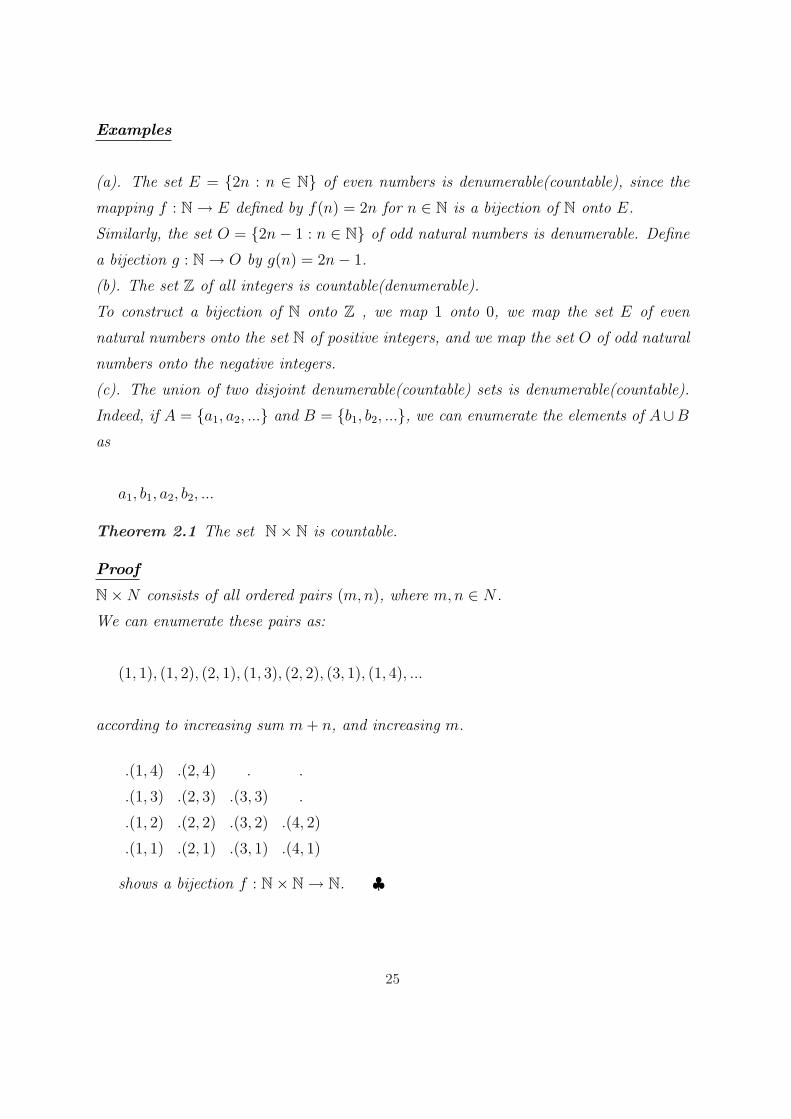
Theorem 2.1 The set N× N is countable.

Proof

N×N consists of all ordered pairs (m,n), where m,n ∈ N .

We can enumerate these pairs as:

(1, 1), (1, 2), (2, 1), (1, 3), (2, 2), (3, 1), (1, 4), ...

according to increasing sum m + n, and increasing m.

.(1, 4) .(2, 4) . .

.(1, 3) .(2, 3) .(3, 3) .

.(1, 2) .(2, 2) .(3, 2) .(4, 2)

.(1, 1) .(2, 1) .(3, 1) .(4, 1)

shows a bijection f : N× N→ N. ♣

25

Theorem 2.2 Suppose S and T are sets and that T ⊆ S.

(a). If S is a countable set, then T is a countable set

(b). If T is an uncountable set, then S is an uncountable set.

Examples

1. N is countable.

Consider the identity map i : N → N, i.e i(n) = n ∀n ∈ N. Then i is one-to-one

and onto. Thus i is a one-to-one correspondence from the set N onto itself. Hence N is

countable.

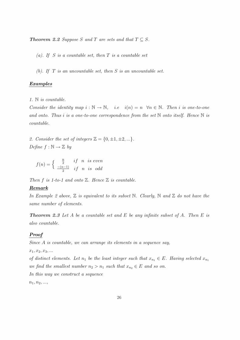
2. Consider the set of integers Z = 0,±1,±2, ....Define f : N→ Z by

f(n) = n

2if n is even

−(n−1)2

if n is odd

Then f is 1-to-1 and onto Z. Hence Z is countable.

Remark

In Example 2 above, Z is equivalent to its subset N. Clearly, N and Z do not have the

same number of elements.

Theorem 2.3 Let A be a countable set and E be any infinite subset of A. Then E is

also countable.

Proof

Since A is countable, we can arrange its elements in a sequence say,

x1, x2, x3, ...

of distinct elements. Let n1 be the least integer such that xn1 ∈ E. Having selected xn1

we find the smallest number n2 > n1 such that xn2 ∈ E and so on.

In this way we construct a sequence

n1, n2, ...,

26

and have the elements

xn1 , xn2 , ...

all belonging to E.

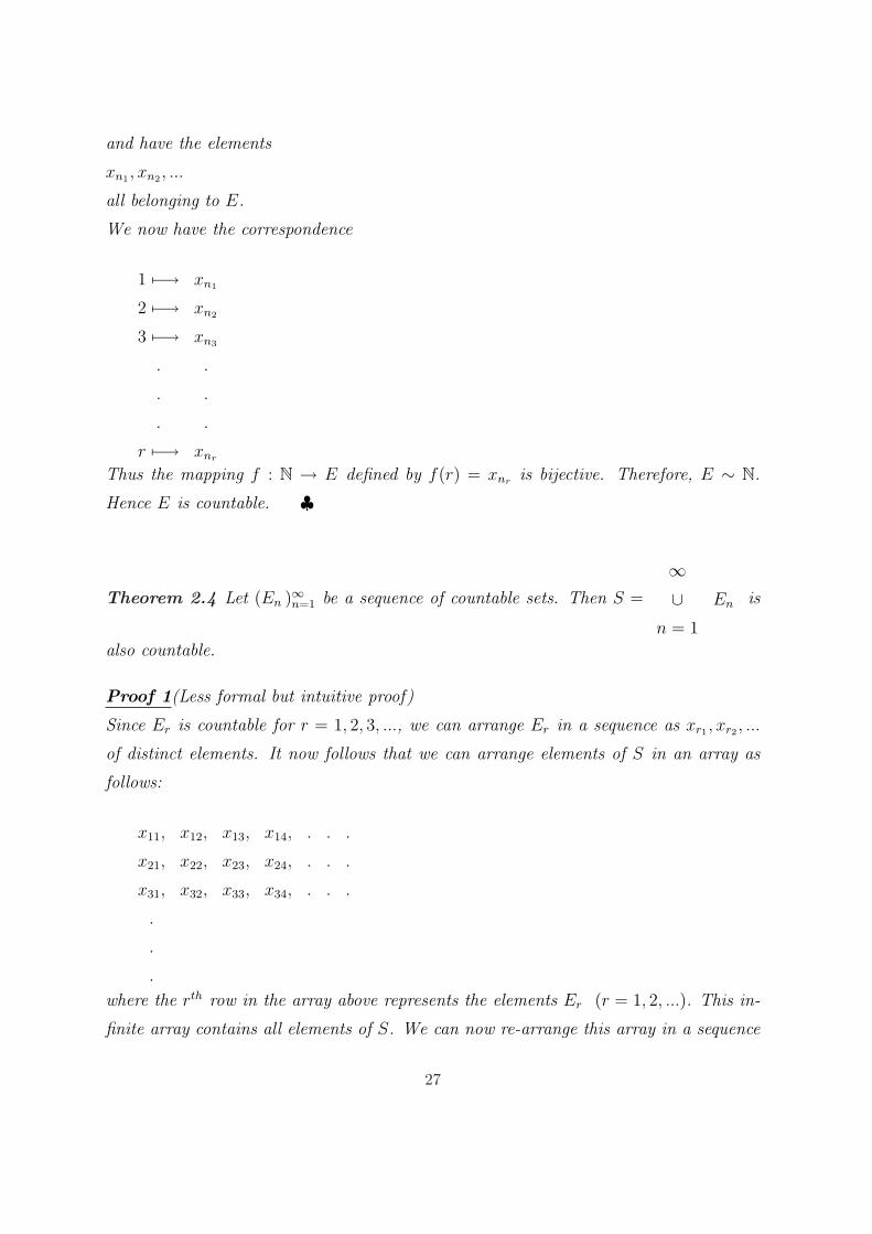
We now have the correspondence

1 7−→ xn1

2 7−→ xn2

3 7−→ xn3

. .

. .

. .

r 7−→ xnr

Thus the mapping f : N → E defined by f(r) = xnr is bijective. Therefore, E ∼ N.

Hence E is countable. ♣

Theorem 2.4 Let (En )∞n=1 be a sequence of countable sets. Then S =

∞∪ En

n = 1

is

also countable.

Proof 1(Less formal but intuitive proof)

Since Er is countable for r = 1, 2, 3, ..., we can arrange Er in a sequence as xr1 , xr2 , ...

of distinct elements. It now follows that we can arrange elements of S in an array as

follows:

x11, x12, x13, x14, . . .

x21, x22, x23, x24, . . .

x31, x32, x33, x34, . . .

.

.

.

where the rth row in the array above represents the elements Er (r = 1, 2, ...). This in-

finite array contains all elements of S. We can now re-arrange this array in a sequence

27

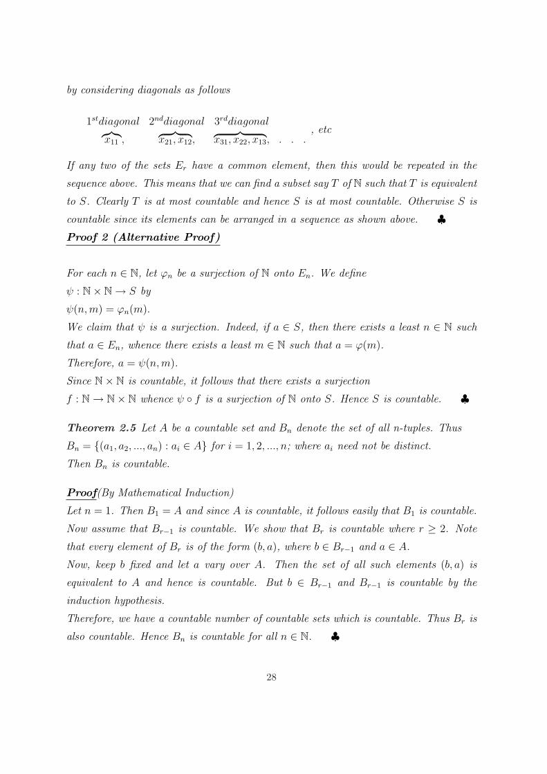
by considering diagonals as follows

1stdiagonal 2nddiagonal 3rddiagonal︷︸︸︷x11 ,

︷ ︸︸ ︷x21, x12,

︷ ︸︸ ︷x31, x22, x13, . . .

, etc

If any two of the sets Er have a common element, then this would be repeated in the

sequence above. This means that we can find a subset say T of N such that T is equivalent

to S. Clearly T is at most countable and hence S is at most countable. Otherwise S is

countable since its elements can be arranged in a sequence as shown above. ♣Proof 2 (Alternative Proof)

For each n ∈ N, let ϕn be a surjection of N onto En. We define

ψ : N× N→ S by

ψ(n,m) = ϕn(m).

We claim that ψ is a surjection. Indeed, if a ∈ S, then there exists a least n ∈ N such

that a ∈ En, whence there exists a least m ∈ N such that a = ϕ(m).

Therefore, a = ψ(n,m).

Since N× N is countable, it follows that there exists a surjection

f : N→ N× N whence ψ f is a surjection of N onto S. Hence S is countable. ♣

Theorem 2.5 Let A be a countable set and Bn denote the set of all n-tuples. Thus

Bn = (a1, a2, ..., an) : ai ∈ A for i = 1, 2, ..., n; where ai need not be distinct.

Then Bn is countable.

Proof(By Mathematical Induction)

Let n = 1. Then B1 = A and since A is countable, it follows easily that B1 is countable.

Now assume that Br−1 is countable. We show that Br is countable where r ≥ 2. Note

that every element of Br is of the form (b, a), where b ∈ Br−1 and a ∈ A.

Now, keep b fixed and let a vary over A. Then the set of all such elements (b, a) is

equivalent to A and hence is countable. But b ∈ Br−1 and Br−1 is countable by the

induction hypothesis.

Therefore, we have a countable number of countable sets which is countable. Thus Br is

also countable. Hence Bn is countable for all n ∈ N. ♣

28

Corollary 2.6 The set Q of all rational numbers is countable.

Proof(Method 1)

We first note that every rational number can be expressed in the form ab

where a, b ∈Z, b 6= 0 and (a, b) = 1.

Consider the ordered pair (a, b) and identify it with ab, i.e. the map

ψ : (a, b) → ab

is a one-to-one correspondence. But the set (a, b) : a, b ∈ Z = Bn

with n = 2 and hence is countable by the previous theorem. Thus we have that B2 ∼ Q.

Hence Q is also countable. ♣

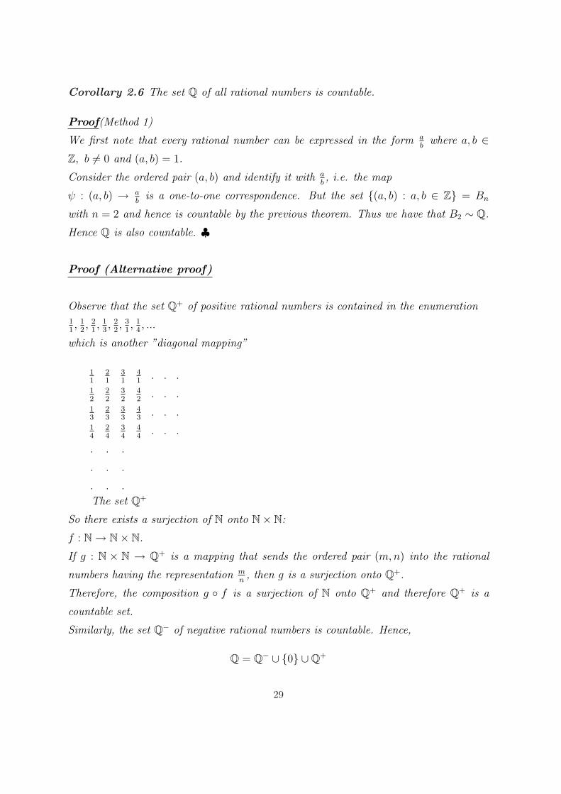
Proof (Alternative proof)

Observe that the set Q+ of positive rational numbers is contained in the enumeration11, 1

2, 2

1, 1

3, 2

2, 3

1, 1

4, ...

which is another ”diagonal mapping”

11

21

31

41

. . .12

22

32

42

. . .13

23

33

43

. . .14

24

34

44

. . .

. . .

. . .

. . .

The set Q+

So there exists a surjection of N onto N× N:

f : N→ N× N.

If g : N × N → Q+ is a mapping that sends the ordered pair (m,n) into the rational

numbers having the representation mn, then g is a surjection onto Q+.

Therefore, the composition g f is a surjection of N onto Q+ and therefore Q+ is a

countable set.

Similarly, the set Q− of negative rational numbers is countable. Hence,

Q = Q− ∪ 0 ∪Q+

29

is countable. ♣

Remark

Since Q contains N, it must be denumerable since N is.

This argument that Q is countable was first given in 1874 by Georg Cantor (1845−1918).

He was the first mathematician to examine the concept of infinite set in rigorous detail.

He also proved that the set of real numbers R is an uncountable set.

2.3 THE UNCOUNTABILITY OF R

Theorem 2.7 Let A be the set of all infinite sequences whose terms consist of only 0

and 1. Then A is uncountable.

Proof

Consider E as a countable subset of A. Enumerate E as a sequence:

s1, s2, ..., sn, ...

We construct an infinite sequence S as follows: The nth member of S is 1 if the nth

member of sn is 0 and vice versa for n = 1, 2, 3, ...

Thus we have that:

S = 1 if sn 6= 1

0 if sn 6= 0

where sn is any member of E.

Clearly, s differs from every member of E. Thus s is not in E and yet s ∈ A.

Hence E is a proper subset of A.

Thus every countable subset of A is a proper subset of A. In this case A must be

uncountable for if it was countable then it would be a proper subset of itself. This is an

absurdity. Hence the result. ♣

Remark

Every real number when expressed in binary uses only the digits 0 and 1. This means

that every real number can be viewed as one of the sequences of A. Thus A constitutes

30

the set of real numbers. Hence R is uncountable. The set QC of irrational numbers is

uncountable.

Proof

We know that Q is countable. Now assume QC is also countable. Then this implies

that R = Q ∪ QC is countable since a union of countable sets is again countable. But

R = Q ∪QC is uncountable by the theorem above. This leads to a contradiction. Hence

QC is uncountable.♣

2.3.1 INTERVALS ON THE REAL LINE

The order relation on R determines a natural collection of subsets called intervals.

Definition 2.6 Bounded Intervals

If a, b ∈ R satisfy a < b, then

(a, b) = x ∈ R : a < x < b is the open interval between a and b.

[a, b] = x ∈ R : a ≤ x ≤ b is the closed interval between a and b.

[a, b) = x ∈ R : a ≤ x < b

(a, b] = x ∈ R : a < x ≤ bare the half-open (or half-closed) intervals between a and b.

Definition 2.7 Unbounded Intervals

The infinite open intervals are:

(a,∞) = x ∈ R : x > a

(−∞, b) = x ∈ R : x < bThe infinite closed intervals are:

[a,∞) = x ∈ R : x ≥ a

(−∞, b] = x ∈ R : x ≤ b

31

Remark

It is often convenient or customary to think of the entire R as an infinite interval, and

write R = (−∞,∞).

Note that −∞ and ∞ are not elements in R, but only convenient symbols.

2.3.2 Nested Intervals

Definition 2.8 A sequence of intervals In, n ∈ N is nested if the following chain of

inclusions holds

I1 ⊇ I2 ⊇ I3 ⊇ ... ⊇ In ⊇ In+1 ⊇ ...

Figure 2.1: Nested intervals

Example If In = [0, 1n], for n ∈ N, then In ⊇ In+1 for each n ∈ N, so this sequence of

intervals is nested.

2.3.3 Nested Interval Property

Theorem 2.8 [Nested Interval Property]

If In = [an, bn], n ∈ N is a nested sequence of closed and bounded intervals, then there

exists a number ξ ∈ In for all n ∈ N.

32

Application of the Nested Interval Property We use the Nested Interval Property

to prove that the set R of real numbers is an uncountable.

Theorem 2.9 The set R of real numbers is not countable.

Proof

It suffices to prove that the unit interval I = [0, 1] is an uncountable set. This implies

that the set R is an uncountable set, for if it were countable, then the subset I would

also be countable. We prove by contradiction.

Assume that I is countable. Then we can enumerate the set as I = x1, x2, ..., xn, ....We first select a closed subinterval I1 of I such that x1 6∈ I1, then select a closed interval

I2 of I1 such that x2 6∈ I2, and so on. In this way, we obtain nonempty closed intervals

I1 ⊇ I2 ⊇ I3 ⊇ ... ⊇ In ⊇ ...

such that In ⊆ I and xn 6∈ In for all n.

The Nested Intervals Property implies that there exists a point ξ ∈ I such that ξ ∈ In for

all n. Therefore ξ 6= xn for all n ∈ N, so the enumeration of I is not a complete listing

of the elements of I, as claimed. Hence, I is an uncountable set. Since I is equivalent

to R (see Exercise below), it follows that R is uncountable. ♣

Exercise: Find a one-to-one correspondence f : R −→ [0, 1].

Cardinality of subsets of R

If two sets A and B are equivalent, then they have the same cardinality or the same

cardinal number.

Definition 2.9 If A is finite, then cardinality of A is the number of elements in A.

Remarks

The cardinal number of a countable set A is denoted by the symbol ℵ0 and is called aleph

zero or aleph nought or aleph null and written

Card A = ℵ0.

Since every infinite subset of a countable set is also countable, it follows that the count-

able infinity is the smallest infinity among infinities of all orders.

33

It therefore follows that infinity of an uncountable set like R is of a higher order than

that of a countable set like Q of rationals.

Example

Given the following limits

1. limn→∞

n2 = ∞

2. limn→∞

2n = ∞

We note that the infinity generated by the limit in part (2) is of a higher order than the

infinity generated by the limit in part (1).

Definition 2.10 A set A is said to have a cardinal number less than of another set B

if A is equivalent to a proper subset of B but A is not equivalent to B.

Thus Card A < Card B.

Theorem 2.10 Let M be an infinite set and P(M) denotes the class of all subsets of

M . Then we have that:

Card M < Card P(M).

Proof

Let M = a, b, c, .... Then in particular the singleton subsets

a, b, c, ... ∈ P(M).

Thus the mapping

a 7−→ ab 7−→ b. . .

is a one-to-one correspondence.

It follows that M is equivalent to a proper subset of P(M) that contains only single-

tons. Note that P (M) contains other subsets like b, a, b, c, a, c, etc. which are not

mapped to under this correspondence. Thus M is not equivalent to P(M).

34

Hence by definition, Card M < CardP(M). ♣

Example

If M is a finite set and thus has n elements then Card M = n. But we have

Card(P(M)) =

(n

0

)+

(n

1

)+

(n

2

)+ · · ·+

(n

n

)= 2n

Clearly 2n > n.

Thus the theorem is equally true for the case of finite sets.

Exercise

Given M = x, y, z, write down all the elements of P(M).

Remarks

The concept of countability of a set is equivalent to the concept of nextness of a set.

This is why every countable set can be enumerated as a sequence.

The cardinality of an infinite set is infinity and all those cardinalities which are infinity,

the one involving a countable set is the smallest (i.e. of least order).

SOLVED PROBLEMS

(1). Show that the set Z of integers is countable. Hence deduce that the set of all negative

whole numbers is countable.

Solution

We first show that the set Z is countable.

Define a mapping

f : N 7−→ Z as follows:

f(n) =

n2, if n is even

−(n−1)2

, if n is odd

Clearly f is one-to-one and onto. Thus Z is equivalent to N. Hence Z is countable.

We now show that the set of all negative whole numbers is also countable.

Firstly, note that the required set here is an infinite subset of Z. By Theorem 2.3: An

35

infinite subset of a countable set is again countable, we can conclude that the set of all

negative whole numbers is also countable. ♣

(2). Show that the set of all polynomials with integral coefficients is countable.

Solution

A polynomial of degree n with integral coefficients can be expressed in the form

p(x) = a0 + a1x + a2x2 + a3x

3 + . . . + anxn,

with a0, a1, . . . , an as integers.

Now, the set of (n + 1) tuples (a0, a1, . . . , an) : ai ∈ Z is denoted by Bn+1 and is

countable as seen in Theorem 2.5.

Thus the collection of all polynomials Pn of degree n with integral coefficients can be put

in a one-to-one correspondence with the set Bn+1. In this case, the mapping

f : Pn 7−→ Bn+1

is one-to-one and onto. Hence the collection of such Pn is also countable. But n is any

positive integer, i.e. P1, P2, . . . , Pn, are countable sets. Thus P =

∞∪ Pn

n = 1

is also

countable.

Hence the set of all polynomials of any degree with integral coefficients is countable. ♣

(3). It is well known that a real root to f(x) = 0 when f(x) is a polynomial with rational

coefficients, is called an algebraic number and that the set of all algebraic numbers is

countable.

Given that a real number is called transcendental if it is not algebraic, determine whether

the set of all transcendental numbers is countable or uncountable.

Solution

Let A be the set of all transcendental numbers and B be the set of all algebraic numbers.

36

Then we have that R = A ∪B.

Now, B is countable and R is known to be uncountable. Assume A is countable. Thus

A∪B is countable, since the union of countable sets is again countable. Thus A∪B = Ris countable. This is a contradiction, since R is known to be uncountable. Hence the set

of all transcendental numbers is uncountable. ♣

4. Prove that every subset of a countable set is countable.

Proof

Follows easily from Theorem 2.3.

Alternative Proof Let E = xn be a countable set, and let A be a subset of E. If A

is empty, A is countable by definition. If A is not empty, choose x ∈ A. Define a new

sequence yn by setting

yn =

xn, if xn ∈ A

x, if xn 6∈ A

Then A is the range of yn and is therefore countable.

5. Let A be a countable set. Prove that the set of all finite sequences from A is also

countable.

Proof

Since A is countable, it can be put into a one-to-one correspondence with a subset of the

set N of natural numbers. Thus it suffices to prove that the set of all finite sequences

of natural numbers is countable. Let 2, 3, 5, 7, 11, · · · , pk · · · be the sequence of prime

numbers. Then each n in N has a unique factorization of the form

n = 2x13x2 · · · pxkk ,

where xi ∈ N0 = N ∪ 0 = W and xk > 0.

Let f be the function on N that assigns to the natural number n the finite sequence

x1, · · · , xk from N0. Then S is a subset of the range of f . Hence S is countable by

Problem 4 above.

Tutorial Problems

37

1. Show that the set Ω = N − 2, 4, · · · , 2n, · · · is countable, where N denotes the set

of natural numbers.

2. Prove that the set N× N is countable by identifying a bijection f : N× N −→ N.

3. Show that the set S = 12, 22, 32, · · · of the squares of the positive integers is count-

able.

4. Let A and B be sets such that A is countable and B is uncountable. Prove that B−A

is uncountable.

5. Prove that the set Q of rational numbers is countable by identifying a bijection from

a countable set to Q.

6. Let A and B be countable sets. Prove that Aand B are equivalent.

7. Prove that the set of all polynomials in x with rational coefficients is countable.

8. Prove that (0, 1) ∼ (a, b). [Hint: f : (0, 1) −→ (a, b) defined by f(x) = a + x(b− a)

is a bijection of (0, 1) onto (a, b)]

9.(a). Prove that (0, 1) ∼ (0, 1]. [ This problem is not easy! Hint: Consider the func-

tion on (0, 1) that for each n ∈ N, n ≥ 2, maps 1n

to 1n−1

, and is the identity mapping

elsewhere]

(b). Prove that (0, 1) ∼ [0, 1] and hence deduce that [0, 1] ∼ R.

38

Chapter 3

STRUCTURE OF THE METRIC

SPACE R

3.1 Introduction

The system of real numbers has two types of properties. The first type which consists

of the algebraic, dealing with addition and multiplication, etc was studied in Chapter

one. In this Chapter we concentrate on another aspect of the real numbers-the concept

of distance, which is fundamental in classical analysis. The latter properties are called

topological or metric. The results of this chapter will come in handy in the rest of the

chapters in this course. For instance, the classical definition of continuity:

f : R 7−→ R is continuous at x ∈ R, if given ε > 0, then for some δ > 0,

|f(x)− f(y)| < ε whenever |x− y| < δ, for y ∈ R

can be crudely restated (using | x− y | as a measure of distance between x and y) as:

”f is continuous at x if f(y) is near to f(x) whenever y is near enough to

x”.

In this chapter, we furnish R with a geometric structure which provides for the concept

of distance between any two given elements of R. We endow R with a metric (which is

an abstraction of a distance function) and hence refer to it as a metric space.

39

We will discuss the concepts of an ε− neighborhood of a point, open and closed sets and

later apply the results to convergence of sequences and continuity of functions defined on

metric spaces. We will define the notions of ”convergence of a sequence” and ”limit of

a set” in terms of ε−neighbouhoods.

3.2 The notion of a metric

Definition 3.1 A metric on a non-empty set X is a function

d : X ×X −→ Rthat satisfies the following properties:

(i). d(x, y) ≥ 0 for all x, y ∈ X. [positivity]

(ii). d(x, y) = 0 iff x = y [definiteness or nondegeneracy]

(iii). d(x, y) = d(y, x) for all x, y ∈ X [symmetry]

(iv). d(x, y) ≤ d(x, z) + d(z, y) for all x, y, z ∈ X [triangle inequality]

A set X equipped with a metric d, and denoted (X, d) is called a metric space. That is,

a metric space is a set X with a metric defined on it.

Remark:

There are always many different metrics for a given set X.

3.2.1 Examples of Metrics

1. The usual or familiar or standard metric for R is defined by

d(x, y) =| x− y |, for all x, y ∈ R.

We show that d is a metric by running all the axioms of a metric:

(i). d(x, y) =| x− y |≥ 0, for all x, y ∈ R.

40

(ii). d(x, y) = 0 ⇐⇒ |x− y| = 0

⇐⇒ x− y = 0

⇐⇒ x = y, ∀ x, y ∈ R(iii). d(y, x) = |y − x| = | − (x− y)|

= | − 1||x− y|= |x− y|= d(x, y) ,∀ x,y∈ R

(iv). follows from the triangle inequality for absolute values because we have

d(x, y) = |x− y| = |(x− z) + (z − y)|≤ |x− z|+ |z − y| = d(x, z) + d(z, y)

d(x, z) = |x− z| = |x− y + y − z|≤ |x− y|+ |y − z|= d(x, y) + d(y, z), ∀ x, y, z ∈ R

Thus d is a metric on R and hence (R, d) is a metric space.

2. The discrete metric. If X is a non-empty set, define d by

d(x, y) =

1 if x 6= y

0 if x = y

Exercise: Verify that d in (2) above is a metric on X.

Solution

Note that the first three properties follow easily. The triangle inequality does not hold if

d(x, y) = 1 and d(x, z) = d(y, z) = 0. However, this would only be possible for x = y = z.

Hence, d(x, y) cannot be equal to 1. This proves that

d(x, y) ≤ d(x, z) + d(y, z), ∀ x, y, z ∈ X.

Remark

41

We note that if (X, d) is a metric space, and T ⊆ S, then d′ defined by d′(x, y) := d(x, y),

for all x, y ∈ T gives a metric on T , which we generally denote by d and say that (T, d)

is a metric space. For instance, the standard metric on R is a metric on the set Q of

rational numbers, and thus (Q, d) is also a metric space.

In general, suppose that (X, d) is a metric space and A is a non-empty subset of X. If

x and y are in A, d(x, y) is the distance between x and y in the metric space (X, d),

and clearly d generates a notion of distance between points in the set A. However (if

A 6= X), d is not a metric for A because a metric for A is a function on A×A while d

is a function on X × Y . This defect can be remedied as follows:

Let dA be the restriction of d to A×A. Then it is easy to verify that dA is a metric for

A, called the relative metric induced by d on A. The metric space (A, dA) is called the

subspace of (X, d) generated by A. Despite the formalism, the idea is very simple; the

distance between two points in (A, dA) is precisely the distance between them in (X, d).

However, despite the simplicity of the idea, some care is required when working with

relative metrics; a subspace may have properties quite different from the original space.

We now present some basic definitions and theorems about metric spaces.

3.3 Neighbourhoods, Interior points and Open sets

There are special types of sets that play a distinguished role in analysis. These are the

open and closed sets in R. To expedite this discussion, it is convenient to have sound

grip of the notion of a neighbourhood of a point.

This is the basic notion needed for the introduction of limit concepts.

3.3.1 Neighborhoods in a metric space

Definition 3.2 Let (X, d) be a metric space. Then for ε > 0, the open ε−neighbourhoodof a point x0 in X is the set

Vε(x0) = x ∈ X : d(x0, x) < ε

42

Other names are: the open ε−ball centre x0, an open disc with centre x0 and

radius ε or simply a neighbourhood of x0, or a sphere, if precision is not required.

In R with its usual metric, an open sphere centred at p radius ε is the set

Sε(p) = x ∈ R : |x− p| < ε.

This consists of all those real numbers x which satisfy the inequality

−ε < x− a < ε ⇐⇒ p− ε < x < p + ε

Remark We note that spheres in various metric spaces can look quite different from

those in Euclidean space. It should be particularly noticed that the spheres in a given

sphere may be quite unlike those in a subspace.

Definition 3.3 Let x0 ∈ (R, d) be a fixed element and r > 0 be a real number, where d

is the usual metric on R. Then the set given by

N(x0, r) = x ∈ R : |x− x0| < r

is called the open neighbourhood (nbhd) of x0 centered at x0 with radius r.

43

Graphically, N(x0, r) looks like

Figure 3.1: N(x0, r)

This nbhd is the open interval (x0 − r, x0 + r).

Definition 3.4 Let A be a subset of R. A point x ∈ A is said to be an interior point

of A if there exists a neighbourhood N(x, r) for some r > 0 such that N(x, r) ⊂ A.

That is, N(x, r) is properly contained in A.

Example

Let A ⊆ R be given by A = x ∈ R : 0 < x < 1. Then an element like 14∈ A is an

interior point of A since N(14, 1

8) ⊂ A. But the element 1 is not an interior point of A

since there does not exist a neighbourhood N(1, r) such that N(1, r) ⊂ A.

Definition 3.5 Let A be a subset of R. The set of interior points of A is called the

interior of A and is denoted by A or int(A).

That is

int(A) = x : x is an interior point of A.

Example

Let A = x ∈ R : 0 < x ≤ 1. Then int(A) = x ∈ R : 0 < x < 1

44

Remark Clearly, int(A) ⊆ A.

Definition 3.6 A point x ∈ R is said to be a boundary point of A ⊆ R if every nbhd

N(x, r), r > 0 of x contains points in A and points in AC.

Definition 3.7 The boundary of a set A ⊆ R, usually denoted by ∂A, or B′dary(A)

is the collection of all the boundary points of A.

Remark Clearly x ∈ ∂A iff for all r > 0 N(x, r) ∩ A 6= ∅ and N(x, r) ∩ AC 6= ∅.Exercise: Show that a set A and its complement AC have exactly the same boundary

points.

That is: ∂A = ∂AC.

Definition 3.8 Let A be a subset of R. Then A is said to be open in R if every

element of A is an interior point of A. In other words, a subset A ⊆ R is said to be

open in R if for each x ∈ A, ∃ a nbhd N(x, r) of x radius r > 0 such that N(x, r) ⊂ A.

Remark Note that the interior of a set is always an open set. Examples

1. The set G = x ∈ R : 0 < x < 1 is open.

Proof

For any x ∈ G we may take rx to be the smaller of the numbers x, 1− x. It is left as an

exercise to show that if |u− x| < rx, then u ∈ G.

Alternative Proof

Follows easily since every member of G is an interior point of G.

2. The set R = (−∞,∞) is open.

Proof

For any x ∈ R, we may take r = 1. That is R is an open set.

3. Generally any open interval I = (a, b) is an open set.

In fact, if x ∈ I, we can take rx to be the smaller of the numbers x− a, b− x.

45

Exercise: Show that (x− rx, x + rx) ⊂ I.

Similarly, the intervals (−∞, b) and (a,∞) are open sets.

4. The set A ⊆ R given by A = x ∈ R : 0 < x ≤ 1 is not open since the element

1 ∈ A but 1 is not an interior point of A.

5. It is easy to prove that:

(i) int(N) = ∅

(ii). int(Q) = ∅

(iii). int(QC) = ∅

(iv). int(x) = ∅

(v). int(R) = R

3.4 Limit Points and Closed sets

Definition 3.9 Let A be a subset of R. A point x ∈ R is said to be a limit point or

a cluster point or an accumulation point of A if every nbhd of x has at least one

element of A different from x or equivalently, if every nbhd N(x, r) of x has infinitely

many points.

Remarks

• Clearly, x is a limit point of A iff for every open nbhd, N(x, r) of x, we have

N(x, r) ∩ A 6= ∅.• If x ∈ R, the definition demands that N(x, r) should contain at least one other point

of A.

46

Example: Let A ⊆ R be given by A = x ∈ R : 0 < x < 1. Then an element 12∈ A is

a limit point of A; i.e. N(12, r) ∩ A 6= ∅ for any r > 0. Also, the 1 ∈ R is a limit point

of A since N(1, r) ∩ A 6= ∅ for any r > 0.

Remarks

1. Note that a limit point of a set may or may not belong to the set.

2. If there is a member of a set which is not a limit point of the set, then it is called an

isolated point of the set.

Definition 3.10 The set of all the limit points of a set A, usually denoted by A′is

called the derived set of A.

That is, A′= x : x is a limit point of A.

Definition 3.11 A subset A of R is said to be closed if every limit point of A belongs

to A.

That is, A is closed if AC is open in R. To show that A ⊆ R is closed, it suffices to

show that each point y of A has an open neighborhood N(x, r) disjoint from A.

Examples

1. The set I = [0, 1] is closed in R.

To see this, let y 6∈ I; then either y < 0 or y > 1. If y < 0, we take εy = |y|, and if

y > 1, take εy = y − 1.

Exercise: Show that in either case, we have I ∩ (y − εy, y + εy) = ∅.Alternatively, show that every limit point of I belongs to I. ♣

2. The set H = x ∈ R : 0 ≤ x < 1 is neither open nor closed.

3. The set A = x ∈ R : 0 < x ≤ 1 is not closed in R since 0 is a limit point of A but

0 6∈ A.

47

4. The empty set ∅ is open in R. In fact the empty set contains no points at all, so the

requirement in the definition is vacuously verified. The empty set is also closed since its

complement R is open.

Definition 3.12 Let A be a subset of R. Then the closure of A, denoted by A or

cl(A) is given by

A = A ∪ x : x is a limit point of A = A ∪ A′.

Remark

Clearly A ⊆ A.

Example

Let A = x ∈ R : 0 < x ≤ 1. Then

A = A⋃0 = x ∈ R : 0 ≤ x ≤ 1 = [0, 1].

Remark: We established that Q and QC are dense in R. We give a more rigorous

definition of a dense set:

Definition 3.13 A subset A of R is said to be dense in R if every limit point of Ris also a limit of A.

That is if A = R.

Thus, we have Q = R, and QC = R.

That is if p is any real number, then every nbhd of p contains at least one rational

number and it also contains at least one irrational number.

Theorem 3.1 Let A be a subset of R. Then A is closed if and only if AC is open.

Proof

(⇒) Assume A is closed and let x ∈ AC. Then x cannot be a limit point of A for if it

is then x ∈ A, for A is closed. Thus there exists an open nbhd N(x, r) of x such that

N(x, r) ∩ A = ∅.Thus, N(x, r) ⊂ AC. Hence AC is open.

(⇐) Conversely, assume that AC is open and let x be any limit point of A. Then every

open nbhd N(x, r) of x is such that N(x, r) ∩ AC 6= ∅. Thus x cannot be an interior

48

point of AC. Since AC is open (by assumption-and hence doesn’t contain all of its limit

points), x 6∈ AC.

This implies that x ∈ A. Thus every limit point of A belongs to A. Hence A is closed.

3.5 Properties of open and closed sets in R

Theorem 3.2 (a). The union of an arbitrary collection of open subsets in R is open.

(b). The intersection of any finite collection of open sets in R is open.

Theorem 3.3 (a). The intersection of an arbitrary collection of closed sets in R is

closed.

(b). The union of any finite collection of closed sets in R is also closed.

Examples

(1). Let Gn = (0, 1 + 1n), for n ∈ N. Then Gn is open for each n ∈ N.

However, the intersection

G =

∞∩ Gn

n = 1

= (0, 1], which is not open in R.

Thus, the intersection of infinitely many open sets in R need not be open

(2). Let Fn = [ 1n, 1], for n ∈ N. Each Fn is closed, but the union

F =

∞∪ Fn

n = 1

= (0, 1], which is not closed in R. Thus, the union of infinitely

many closed sets in R need not be closed.

Theorem 3.4 A subset of A ⊂ R is closed if and only if it contains all its limit points.

Proof

(⇒) Let A be a closed subset of R and let x be a limit point of A. We will show that

x ∈ A. For a contradiction suppose that x 6∈ A. Then x ∈ AC, an open set. Therefore,

there exists an open neighbourhood N(x, r) of x such that N(x, r) ⊂ AC.

Consequently, N(x, r) ∩A = ∅, which contradicts the assumption that x is a limit point

49

of A. Thus A must contain all of its limits points.

(⇐) Conversely, let A be a subset of R that contains all of its limit points. We show

that A is closed. It suffices to show that AC is open. For if y ∈ AC, then y is not a

limit point of A. It follows that ∃ an open nbhd N(y, r) of y that does not contain a

point of A. (except possibly y).

But since y ∈ AC, it follows that N(y, r) ⊂ AC. Since y is an arbitrary element of AC,

we deduce that for every point in AC, there exists an open nbhd that is entirely contained

in AC. But this means that AC is open in R. Therefore A is closed in R. ♣

Theorem 3.5 A subset of R is open if and only if it is the union of countably many

disjoint open intervals in R.

Remark It does not follow from the above theorem that a subset of R is closed iff it is

the intersection of a countable collection of closed intervals ( why not?). In fact, there

are closed sets in R that cannot be expressed as the intersection of a countable collection

of closed intervals in R. A set consisting of two points is one example( why?).

3.6 Relatively Open and Closed Sets

One of the reasons for studying topological or metric concepts is to enable us to study

properties of continuous functions. In most instances, the domain of a function is not

all of R, but rather a proper subset of R. When discussing a particular function we will

always restrict our attention to the domain of the function rather than all of R. With

this in mind, we make the following definition.

Definition 3.14 Let X be s subset of R.

(a). A subset U of X is open in (or open relative to) X if for every p ∈ U , there

exists an r > 0 such that N(p, r) ∩X ⊂ U .

(b). A subset C of X is closed in (or relative to) X if X − C is open in X

Example. Let X = [0,∞) and let U = [0, 1). Then U is not open in R but is open in

X.(Why?)

The following theorem provides a simple characterization of what it means for a set to

be open or closed in X.

50

Theorem 3.6 Let X be a subset of R.

(a). A subset U of X is open in X if and only if U = X ∩O for some open subset O of

R.

(b). A subset C of X is closed in X if and only if C = X ∩ F for some closed subset F

of R.

Remark

Clearly, open(closed) =⇒ relatively open ( relatively closed) but the converse is not gen-

erally true.

3.7 Solved Problems

1. (a). Give the definition of an open subset of R and a closed subset of R.

(b). Let A ⊆ R be given by A = x ∈ R : 1 ≤ x < 2. Show that A is neither closed nor

open.

Solutions

(a). A subset A of R is said to be open if every member of A is an interior point of A.

But A is said to be closed in R if every limit point of A belongs to A.

(b). A = x ∈ R : 1 ≤ x < 2 is not closed since 2 is a limit point of A but 2 6∈ A.

Also A is not open since 1 ∈ A but 1 is not an interior point of A.

2.(a). Construct a set of real numbers with only 3 limits.(Hint: Note that the set

A = 1n

: n ∈ N has only 0 as the limit point.)

(b). Let A ⊆ R. Prove that:

(i). A is open iff A = Int(A)

(ii). A is closed iff A = A.

Solution

(a). Given A = 1n

: n ∈ N, we note thatlim 1

n= 0

n →∞. Now let

51

B = 1 + 1n

: n ∈ N and C = 2 + 1n

: n ∈ N. Similarly sets B and C have only one

limit point each. Thus S = A ∪B ∪ C is a set whose limit points are 0, 1, and 2.

(b). A ⊆ R.

(i). A is open iff A = Int(A).

(⇒) Assume A = Int(A). Then A is open because int(A) is always open.

(⇐) Conversely, assume that A is open. Then for any x ∈ A, we have that x is an

interior point of A. That is x ∈ A =⇒ x ∈ Int(A). Thus

A ⊆ Int(A)

(1)

But the inclusion

Int(A) ⊆ A

(2)

is immediate(obvious).

From (1) and (2) it follows that A = Int(A).

(ii). A is closed iff A = A.

(⇒) Assume that A = A. Then A is closed since A is always closed.

(⇐) Conversely, assume that A is closed. Then every limit point of A belongs to A. But

x is a limit point of A means that x ∈ A.

Thus x ∈ A =⇒ x ∈ A.

That is A ⊆ A

(1)

But the inclusion

52

A ⊆ A

(2)

is obvious.

From (1) and (2) equality follows. That is A = A. ♣

3. Show that the set N of natural numbers is closed in R.

Solution

The complement of N is the union (−∞, 1)∪ (1, 2)∪ · · · of open intervals , hence open.

Therefore, N is closed since its complement is closed.

4. Show that the set Q of rational numbers is neither open nor closed.

Solution

Every nbhd of x ∈ Q contains a point not in Q.

5. Give an example of a set A ⊆ R such that int(A) = ∅ and A = R.

Solution

A = Q or A = QC.

3.8 Tutorial Problems

1. Let A and B be subsets of a metric space X.

(a). Prove that

(i). int(A) ∪ int(B) ⊆ int(A ∪B).

(ii). int(A) ∩ int(B) = int(A ∩B).

(iii). (A ∪B) = A ∪B.

(iv). (A ∩B) ⊆ A ∩B.

53

(b). Give an example of two subsets A and B of R such that

(i). int(A) ∪ int(B) 6= int(A ∪B).

(ii). (A ∩B) 6= A ∩B.

2. Prove that

(a). ∂A = A ∩ AC

(b). ∂A = A− int(A)

3. Find the boundary points of each of the following sets

(a). A = (a, b)

(b). A = 1n

: n ∈ N

(c). A = Q

(d). A = N

(e). A = R

4. (a). Prove that a set A ⊆ R is open if and only if A does not contain any of its

boundary points.

(b). Prove that a set A ⊆ R is closed if and only if A contains all of its boundary points.

54

Chapter 4

BOUNDED SUBSETS OF R

4.1 Introduction

In this chapter we will consider the concept of the least upper bound of a set and introduce

the least upper bound property of the real numbers R. We will show that that this property

fails for the rational numbers Q. We first define the notions of upper bound and lower

bound of a subset of real numbers.

4.2 Upper Bounds, Lower Bounds of a subset of R

Definition 4.1 A non-empty subset S of real numbers is said to be bounded above

and thus has an upper bound, say b if b ≥ x for all x ∈ S.

A non-empty subset S of R is said to be bounded below and thus has a lower bound,

say q if q ≤ x for all x ∈ S.

Remark

1. If b is an upper bound for S then any real number b′ > b is also an upper bound for

S.

In other words, if a set has an upper bound, then it has infinitely many upper bounds,

because b + 1, b + 2, ... are upper bounds of S.

55

2. If q is a lower bound for S, then any real number q′ < q is also a lower bound for S.

Thus, if a set has a lower bound, then it has infinitely many lower bounds, because

q − 1, q − 2, ... are lower bounds of S.

Definition 4.2 A set is said to be bounded if it is both bounded above and bounded

below. A set is said to be unbounded if it is not bounded.

Example The set S = x ∈ R : x < 2 is bounded above; the number 2 and any other

number larger than 2 is an upper bound of S. This set has no lower bounds, so that the

set is not bounded below. Thus it is unbounded (even though it is bounded above !).

In the set of upper bounds of S and set of lower bounds of S, we single out their least

and greatest elements, respectively, for special attention.

4.2.1 Supremum and Infimum of a subset of R

Definition 4.3 Let S be a nonempty subset of R.

(a). If S is bounded above, then a number u is said to be the supremum (or the least

upper bound) of S if it satisfies the conditions:

(1). u is an upper bound of S, and

(2). if v is any other bound of S, then u ≤ v.

That is, if u′ < u, then u′ is not an upper bound of S. Then there exists u′′ ∈ S such

that u′ < u′′ < u.

Definition 4.4 If S is bounded below, then a number w is said to be the infimimum

(or greatest lower bound) of S if it satisfies the conditions:

(1’). w is a lower bound of S, and

(2’). if t is any lower bound of S, then t ≤ w. That is , if q is a lower bound of S and

if q′ > q, then q′ is not a lower bound for S. Thus, ∃ q′′ ∈ S such that q′ > q′′ > q.

Remark

1. It is not difficult to see that there can be only one supremum of a given subset S of R.

Thus we can refer to it as the supremum of S instead of a supremum). For suppose that

u1 and u2 are both suprema of S. If u1 < u2, then the hypothesis that u2 is a supremum,

then this implies that u1 cannot be an upper bound of S. Similarly, we see that u2 < u1

56

is not possible. Therefore, we must have u1 = u2.

A similar argument can be given to show that the infimum of a set is unique.

If the supremum and infimum of a set exists, we will denote them by Sup S and Inf S,

respectively.

We observe that if u′ is an arbitrary upper bound of a non-empty set S, then

Sup S ≤ u′ (because SupS is the least upper bound of S).

2. Note that in order for a nonempty set S in R to have a supremum, it must have an

upper bound. Thus, not every subset of R has a supremum. Similarly, not every subset

of R has an infimum.

Four possibilities for a nonempty subset of R

A subset of R can have:

(1). both a supremum and an infimum,

(2). a supremum but no infimum,

(3). an infimum but no supremum,

(4). neither a supremum nor an infimum.

57

The figure below show the properties of a bounded set.

Figure 4.1: Bounds of S

Examples

1. Let A = x ∈ R : 0 < x < 1. Then

u = lubA = SupA = 1.

If we take any u′ < u, say u′ = 0.9, then ∃ u” say u” = 0.95 ∈ A and 0.9 < 0.95 < 1.

Thus u′ < u” < u.

2. Let B = x ∈ R : 0 < x < 1⋃2. Then u = SupB = 2. If we take u′ = 1.5, then

u′ < b” = b.

Example

Let A = x ∈ R : 0 < x < 1. Then q = glbA = infA = 0. If we take any q′ > q say

q′ = 18

and 0 < 18

< 14.

Thus q′ > q” = q.

Example Let B = x ∈ R : 0 < x < 1⋃−1. Then q = infA = −1. If we let

q′ = −14, say, then q” = −1 = q. Thus q′ > q” > q.

58

Remark

Below are equivalent definitions of sup S and inf S using ε > 0.

Definition 4.5 A real number b is said to be the least upper bound of S if for each

ε > 0, b− ε is not an upper bound for S. For ∃ b′ ∈ S such that b− ε < b′ < b.

Similarly, a real number q is said to be the greatest lower bound for S if for each ε > 0,

q + ε is not a lower bound for S, since ∃ q′ ∈ S such that q + ε > q′ > q.

Remarks

1. From the above definition, it follows that every nbhd of b = sup S or q = inf S has at

least one point of S. Thus b = sup S and q = inf S are limit points of S which need not

belong to S.

2. sup S ∈ S, inf S ∈ S.

3. In the special case when sup S ∈ S and inf S ∈ S, then sup S is called the maximum

element of S while inf S is called the minimum element of S.

Example Let A ⊆ R be given by

A = x ∈ R : 0 < x ≤ 1Then inf A = 0 6∈ A. Hence A has no minimum element. But sup A = 1 ∈ A. Hence 1

is the maximum element of A.

Remark In general some sets of real numbers do not have sup or inf unless bounded

above or below, respectively. The completeness axiom guarantees existence of supremum

and infimum.

We will give an example to show that the claim of completeness axiom is only enjoyed

by set of real numbers but not other sets like those of rational or irrational numbers.

4.3 The Completeness Property of R

Proposition 4.1 (Least Upper Bound Property of R) Every nonempty subset of

real numbers that has an upper bound also has a supremum in R.

59

Remark

This property is called the Supremum Property of R. The analogous property for infima

can be deduced from the Completeness Property as follows:

Every nonempty subset of R that is bounded below has an infimum or greatest lower

bound in R. Every nonempty subset of R that is bounded below has an infimum or

greatest lower bound in R. Suppose that S is a nonempty subset of R that is bounded

below. Then the nonempty set S∗ = −s : s ∈ S is bounded above, and the supremum

property implies that u = SupS∗ exists in R.This can be re-stated as follows:

Proposition 4.2 (The Infimum or Greatest Lower Bound property of R)

Every nonempty subset of R that is bounded below has an infimum or greatest lower

bound in R.

Combining the immediate two propositions we have:

Theorem 4.3 (The Completeness Property of R): Every nonempty subset of real

numbers that has an upper bound also has a supremum in R and every nonempty subset

of R that is bounded below has an infimum or greatest lower bound in R.

Exercise:In the remark above, verify in detail that −u is the inf of S.

We demonstrate that not all subsets of R enjoy the Completeness Property.

Example

Let S = y : y ∈ Q, 0 ≤ y, y2 < 2. Then clearly 0 ∈ S so that S 6= ∅. Now suppose that

s ∈ S, then s2 < 2 and 2 − s2 is a positive rational number. Select a positive rational

number h such that h < 1 and h < 2−s2

2s+1and let u = s + h.

Clearly h is rational and 0 < s < u. Also we can easily check that :

u2 = s2 + 2sh + h2 < s2 + 2sh + h < 2. Hence u ∈ S. That is for any given member of

S, there always exists a larger member of S. Hence S has no largest member.

This result shows that rational numbers do not have the completeness property.

4.4 Solved Problems

1. (a). Give an example of the following:

60

(i). a set S ⊆ R such that SupS = InfS.

(ii). a set S ⊆ R which has got infimum, minimum and supremum but no maximum

element.

(b). Show that if the maximum element of a set S ⊆ R exists then it is unique.

Solution

(a). An example of

(i). a set S such that SupS = InfS.

Let S = x. Then SupS = x and InfS = x.

Hence SupS = InfS.

(ii). a set S of reals which has got infimum, minimum, supremum but no maximum

element:

Let S = x ∈ R : 0 ≤ x < 1.Then 0 = InfS and 0 ∈ S. Thus 0 ie equal to the minimum element in S. We also

have that 1 = SupS. But 1 6∈ S. Hence S has no maximum element.

(b). Let b = MaxS. We show that b is unique. Assume we also have b′ = MaxS. Then

in particular b is an upper bound of S and b′ is the lub of S.

That is

b′ < b

(1)

but we also have that b′ is an upper bound of S while b′ is the least upper bound of S.

That is

b < b′

(2)

From (1) and (2), b = b′.

61

Hence MaxS is unique. ♣

4.(a). State the Completeness property of R.

(b). Let E be a closed and bounded subset of R. Show that sup E and inf E belong

to E.

Solution

(a). A set of reals bounded above has the least upper bound in R and if it is bounded

below then it has the greatest lower bound.

(b). Let E be a closed and bounded subset of R. We show that SupE and InfE belong

to E.

Let b = SupE. Then for each ε > 0, b − ε is not an upper bound of E. Thus there

exists b′ ∈ E such that b− ε < b′ < b

This is equivalent to saying that every nbhd N(b, ε) has at least one element of E. That

is b is a limit point of E. But E is closed, hence it contains all its limit points. Thus

b ∈ E. Thus SupE ∈ E.

Similarly, let q = InfE. Then for each ε > 0, q + ε is not a lower bound of E. Thus

there exists q′ ∈ E such that q < q′ < q + ε.

Thus q is a limit point of E. But E is closed. Hence q = InfE ∈ E. ♣

5. Define a set T by T = z : z ∈ Q and 2 < z2. Show that T has no smallest element.

62

Chapter 5

SEQUENCES OF REAL

NUMBERS

5.1 Introduction

In this chapter we study the properties of a sequence of real numbers. In our study of

sequences we encounter our first serious introduction to the limit process. We begin the

chapter by introducing the notion of convergence of a sequence of real numbers and by

proving the standard limit theorems for sequences normally encountered in calculus. We

use the least upper bound property of R to show that every bounded monotone sequence of

real numbers converges in R. We introduce the notion of subsequences and subsequential

limits and use these to provide a proof of the fact that every Cauchy sequence of real

numbers converges.

Definition 5.1 A sequence is an ordered set of numbers, say a1, a2, ... where each mem-

ber is followed by another according to a given rule. In this case we write the sequence as

an∞n=1 = a1, a2, ..., an, ...

The members a1, a2, .. are called the terms of the sequence. The term an is called the nth

term.

Example

Let an∞n=1 = n2 for all n ∈ N. Then an is a sequence of real numbers whose terms

63

are as follows:

an = 12, 22, 32, ..., n2, ...

The nth term of this sequence is n2.

Remark (1) Note that a sequence can also be defined as a function whose domain is the

set N of natural numbers,e.g. the sequence above, f(n) = n2 for all n ∈ N .

5.2 Convergence of a sequence

Definition 5.2 A sequence xn∞n=1 in R is said to converge if there exists a point

x ∈ R such that for every ε > 0, there exists a positive integer n0 such that

xn ∈ N(x, ε) for all n ≥ n0.

Remark

If this is the case, we say that xn converges to x or that x is the limit of the

sequence xn, and we write:

lim xn = x

n →∞or xn −→ x

If xn does not converge, then xn is said to diverge.

In the definition, the statement xn ∈ N(x, ε) for all n ≥ n0 is equivalent to

|xn − x| < ε for all n ≥ n0

(*)

(*) gives the criterion of convergence of a sequence.

As a general rule, the integer n0 will depend on the given ε.

Remark

From (*), we can restate the criterion of convergence as follows:

5.2.1 Criterion of Convergence

A sequence xn of real numbers converges to a real number x if no matter how small

a positive real number ε is we should be able to find a natural number n0 depending on

ε such that the distance between the terms xn of the sequence and the limit x is always

64

less than ε provided the subscript n is greater than n0.

Example 1 Let xn = 1n. We show that xn∞n=1 converges to 0 in R.

Given ε > 0, there exists a positive integer n0 such that n0ε > 1. Thus for all n ≥ n0,

| 1n− 0| = | 1

n| < ε.

Therefore,lim 1

n= 0

n →∞.

In this example, the integer n0 must be chosen so that n0 > 1ε.

Example 2 If x ∈ R, the sequence xn defined by xn = x for all x ∈ R is the constant

sequence of x. Since |xn − x| = 0 for all n ∈ N, we havelim xn = x.

n →∞Example 3 Consider the sequence 2n+1

3n+2∞n=1. We show that

lim 2n+13n+2

= 23

n →∞.

Since |2n+13n+2

− 23| = 1

3(3n+2)< 1

9n, given ε > 0, choose n0 ∈ N such that n0 > 1

9ε. Then for

all n ≥ n0, |2n+13n+2

− 23| < ε.

Thus the given sequence converges to 23.

Example 4 The sequence xn = 1− (−1)n∞n=1 diverges in R. To prove this, we first

note that for this sequence

|xn − xn+1| = 2 for all n. Suppose xn −→ x for some x ∈ R. Let 0 < ε < 1. Then by

definition of convergence, there exists an integer n0 such that

|xn − x| < ε for all n ≥ n0. But if n ≥ n0, then

2 = |xn − xn+1| ≤ |xn − x|+ |x− xn+1| < 2ε < 2.

This, however, is a contradiction. Thus our assumption that the sequence converges is

false; i.e, the sequence diverges.

65

Example 5 Prove thatlim √n + 1−√n = 0

n →∞.

Solution

First we note that

|√n + 1 − √n| = (

√n+1−√n)

1(√

n+1+√

n)

(√

n+1+√

n)= 1√

n+1+√

n< 1

2√

n. Given ε > 0, we want

to choose n0 such that 12√

n< ε for all n ≥ n0. This is easily verified to be the case if

n0 ∈ N is chosen so that n0 ≥ 14ε2

. With this choice of n0, we now have

|√n + 1−√n| < ε for all n ≥ n0 ♣Example 6Showfromfirstprinciplesthatthesequence

xn = 1 + (−1)n 1n2 for all n ∈ N converges to 1 in R.

Solution

Let ε > 0 be given such that |xn − 1| < ε. Then we have that

|1 + (−1)n 1n2 − 1| < ε

That is |(−1)n 1n2 | < ε

That is |(−1)n|| 1n2 | < ε

That is 1n2 < ε. That is n2 > 1

ε

i.e. n > 1√ε.

In this case if we take n0 = N(ε) = [ 1√ε] + 1, where [x] denotes the largest integer less

or equal to x, then we have found the natural number depending on ε such that

|xn − x| < ε, ∀n ≥ n0(ε).

Hence xn −→ 1. ♣

Remark

Note that in determining n0(ε) we have to add 1 because [ 1√ε] could be 0.

Definition 5.3 A sequence xn in R is said to be bounded if there exists a positive

constant M such that |xn| ≤ M for all n ∈ N.

66

This definition is equivalent to saying that the range of xn : n ∈ N of the sequence

xn is a bounded subset of R or if the terms of xn are trapped between two given real

numbers.

Example 1 Let xn = 1n. Then the range is given by

Range xn = 1, 12, 1

3, ...

Clearly, 0 < xn < 1, ∀ n ∈ N.

Hence xn = 1n ∀ n ∈ N is bounded.

Example 2

Define the terms of a sequence as:

xn =

1 if n is odd

0 if n is even

Then the range of xn = 0, 1. Hence xn is bounded.

Example 3 Let xn = n2 for all n ∈ N . Then range xn = 12, 22, .... Clearly, xn is

not bounded. Thus it is unbounded.

Theorem 5.1 Let xn be a sequence of real numbers. If xn converges then its limit

is unique.

Proof

We prove by contradiction. We assume that the sequence converges but that its limit is

not unique. So suppose the sequence xn converges to two distinct points x, y ∈ R, i.e.

xn −→ x and xn −→ y, and x 6= y.

Thus, using the criterion for convergence we have that for each ε > 0 ∃ N1(ε), N2(ε) ∈ Nsuch that

|xn − x| < ε2

∀ n ≥ N1(ε).

Also

|xn − y| < ε2

∀ n ≥ N2(ε).

Let N = maxN1, N2. Then

67

|xn − x| < ε2

∀ n ≥ N and

|xn − y| < ε2

∀ n ≥ N .

By the triangular inequality we have that

|x− y| = |x− xn + xn − y| ≤ |x− xn|+ |xn − y| < ε2

+ ε2

= ε ∀ n ≥ N .

That is |x− y| < ε and ε > 0 is arbitrary. Thus x = y and hence limit of xn is unique

(if it exists).

5.2.2 Bounded Sequences

Theorem 5.2 Let xn be a convergent sequence of real numbers. Then xn is bounded.

Proof

Let xn −→ x. Then x ∈ R. Therefore, for each ε > 0, ∃ n0 ∈ N such that |xn − x| <

ε ∀ n ≥ n0. Since ε > 0 is arbitrary, WLOG(Without loss of generality) we take

ε = 1. Then we have, for this ε:

|xn − x| < 1 ∀n ≥ n0

Let r = min|x1 − x|, |x2 − x|, ..., |xn0−1 − x|, 1Then it follows that:

|xn − x| < r ∀n ∈ N, where r > 0. But we have that

||xn| − |x|| < |xn − x| < r

i.e. ||xn| − |x|| < r, ∀n ∈ N.

In particular, |xn| − |x| < r ∀n ∈ N.

That is |xn| < r + |x|,∀n ∈ N.

Let M = r + |x| > 0. Then |xn| ≤ M ∀n ∈ N. Hence xn is bounded. ♣

Remark We note that the theorem above asserts that:

convergence of xn =⇒ boundedness of xn.But the converse is not true in general as the following example shows:

68

Example 1

Let xn be a sequence of real numbers defined by

xn =

1 if n is odd

0 if n is even

That is xn = 1, 0, 1, 0, ...Then xn is bounded. But xn is not convergent since it oscillates between 0 and 1.

Example 2 The sequence xn = 1− (−1)n∞n=1 is bounded, but the sequence does not

converge. The sequence is bdd since |xn| = |1− (−1)n| ≤ 2 ∀ n ∈ N .

Example 3 The sequence n(−1)n is not bdd in R, and thus cannot converge.

5.3 Subsequences and the Bolzano-Weierstrass Theorem

We prove that every bounded sequence of real numbers has a convergent subsequence.

This is the sequential version of the Bolzano-Weierstrass Theorem.

Definition 5.4 Given a sequence xn in R, consider a sequence nk∞k=1 of positive in-

tegers such that n1 < n2 < n3 < ... Then the sequence xnk∞k=1 is called a subsequence

of the sequence xn.

If the sequence xnk converges, its limit is called a subsequential limit of the sequence

xn. Specifically, a point x ∈ R is a subsequential limit of the sequence xn if there

exists a subsequence xnk of xn that converges to x. Also, we say that ∞ is a subse-

quential limit of xn if there exists a subsequence xnk so that xnk

−→∞ as k −→∞.

Similarly for −∞.

Examples

1. Let xn∞n=1 = x1, x2, ... be any sequence of real numbers. If we extract the terms

whose subscripts are even then we have a subsequence:

xnk∞k=1 = xn1 , xn2 , ..., where xn1 = x2, xn2 = x4, xn3 = x6, ...

Therefore xnk = x2, x4, x6, ... is a subsequence of xn.

2. Consider the sequence xn = (1− (−1)n).If n is even, then xn = 0, and if n is odd, then xn = 2. Thus 0 and 2 are subsequential

69

limits of the given sequence.

Exercise Prove that 0 and 2 are the only two subsequential limits of the above sequence.

3. Consider the sequence xn = (−1)n + 1n.

Both 1 and −1 are subsequential limits. If n is even, i.e. n = 2k, then xn = x2k = 1+ 12k

,

which converges to 1. On the other hand, if n is odd, i.e. n = 2k +1, then xn = x2k+1 =

−1 + 12k+1

,

which converges to −1.

This shows that −1 and 1 are subsequential limits.

4. Let xn = 1n ∀ n ∈ N . Then x2n is a subsequence given by

x2n = 12, 1

4, 1

6, ...

We also have that x2n+1 is a subsequence of xn given by x2n+1 = 1, 13, 1

5, ....

Remarks

1. Note that if a subsequence xnk∞k=1 converges to x, then x is called a subsequential

limit.

2. Note that a sequence is a subsequence of itself.

3. Note that a sequence can have subsequential limit without being convergent:

Example

Let xn =

1 if n is odd

−1 if n is even

That is xn = 1,−1, 1,−1, ....Then xn is not convergent since it oscillates between −1 and 1. However, the subse-

quence x2n+1 = 1, 1, 1, ... converges to 1. Thus 1 is a subsequential limit of xn.Hence a subsequence can be convergent without the sequence being convergent.

Remark We state and prove a result that links the concept of a subsequence to the

convergence of the sequence.

Theorem 5.3 Let xn be a sequence of real umbers. Then xn converges to x if and

only if every subsequence of xn also converges to x.

Proof

(⇒) Firstly assume that xn −→ x. Let xnk∞k=1 be any subsequence of xn. As

xn −→ x we have:

70

For each ε > 0 ∃ n0(ε) ∈ N such that

|xn − x| < ε ∀ n ≥ n0(ε).

Take nk > n0(ε). Then clearly

|xnk − x| < ε ∀ nk > n0(ε).

Thus xnk −→ x.

Since xnkwas any subsequence, it follows that xn −→ x =⇒ every subsequence xnk of

xn converges to x.

(⇐) Conversely, assume that every subsequence of xn converges to x. Then xn −→ x

since xn is a subsequence of itself. ♣Examples

1. Consider the sequence

xn =

1 if n is odd

0 if n is even

That is xn = 1, 0, 1, 0, .... Then the subsequence x2n = 0, 0, ... converges to 0 but

the subsequence x2n+1 = 1, 1, 1, ... converges to 1. Now 0 6= 1. Hence xn diverges

in R since its subsequences do not converge to the same limit.

2. Consider the sequence xn = 1n, for all n ∈ N. Then xn −→ 0. The subse-

quence of xn given by x2n = 12, 1

4, 1

6, ... also converges to 0. Also the subsequence

x2n+1 = 1, 13, 1

5, ... converges to 0.

That is every subsequence of this sequence converges to 0 since xn (which is a subse-

quence of itself) converges to 0.

Theorem 5.4 (Bolzano-Weierstrass) Every bounded infinite subset of R has a limit

point.

Remark

The conclusion of the Bolzano-Weierstrass theorem may fail if either hypothesis is re-

moved. For example, a finite set has no limit point. On the other hand, the st N of

natural numbers is an infinite unbounded subset of R with no limit points.

The following corollary is often called the sequential version of the Bolzano-Weierstrass

Theorem.

71

Corollary 5.5 (Bolzano-Weierstrass) Every bounded sequence in R has a conver-

gent subsequence.

5.4 Monotonic Sequences

Definition 5.5 Let xn be a sequence of real numbers. Then we say that:

(i). xn is monotonic increasing (in symbols xn ) if xn ≤ xn+1 ∀ n ∈ N.

(ii). xn is monotonic decreasing (in symbols xn ) if xn ≥ xn+1 ∀ n ∈ N.

We say that xn is monotonic if it is monotonic increasing or monotonic decreasing.

Examples

1. The sequence xn = n2 ∀ n ∈ N = 1, 4, 9, ... is monotonic increasing.

2. The sequence xn = 1n2 ∀ n ∈ N = 1, 1

4, 1

9, ... is monotonic decreasing.

Remark We know that convergence of xn =⇒ boundedness of xn but the converse

is not true in general. But we now show that these two concepts are equivalent in the

case of monotonic sequences. That is

Convergence ⇐⇒ Boundedness if xn is monotonic.

Theorem 5.6 Let xn be a monotonic sequence of real numbers. Then xn is con-

vergent if and only if it is bounded.

Proof

We only prove the case when xn is monotonic increasing. For the other case, the proof

is similar. Let E = range xn. Since xn is bounded it follows that E is also bounded.

Thus E is a set of real numbers bounded above. Let x = lub E. Then xn ≤ x ∀ n ∈ Nand for each ε > 0, ∃ n0(ε) ∈ N such that x− ε < xn0 ≤ x for otherwise x− ε would be

an upper bound.

By monotonicity of xn it follows that

x− ε < xn < x ∀ n ∈ N.

72

Therefore |xn − x| < ε ∀ n ∈ N.

Thus xn −→ x and hence boundedness =⇒ Convergence.

Remark

1. Note that if xn −→ ∞ or xn −→ −∞ as n −→ ∞, we say that xn diverges in Rbecause −∞ and ∞ are not real numbers.

2. If xn and not bounded above then xn −→ ∞ and hence xn diverges. Also if

xn and is not bounded below then xn −→ −∞ and hence diverges.

5.5 Limit Superior and Limit Inferior of a sequence

These two limit operations are very important because unlike the limit of a sequence, the

lim sup and lim inf of a sequence always exist. They come in handy in the study of series

of real numbers and power series.

Let xn be a sequence in R. For each k ∈ N , we define ak and bk as follows:

ak = infxn : n ≥ k,

bk = supxn : n ≥ k.

From the definition, ak ≤ bk for all k.

Furthermore, sequences ak and bk satisfy the following:

ak ≤ ak+1 and bk ≥ bk+1 for all k.

The sequence ak is nondecreasing.

As a consequence the sequence ak is monotone increasing and the sequence bk is

monotone decreasing.

These sequences always have limits in R ∪ −∞,∞.

73

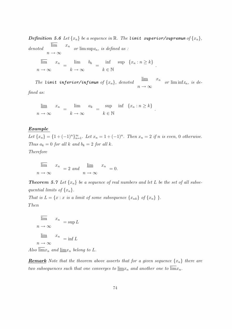
Definition 5.6 Let xn be a sequence in R. The limit superior/supremum of xn,

denotedlim xn

n →∞or lim supxn, is defined as :

lim xn

n →∞=

lim bk

k →∞=

inf sup xn : n ≥ kk ∈ N

.

The limit inferior/infimum of xn, denotedlim xn

n →∞or lim infxn, is de-

fined as:

lim xn

n →∞=

lim ak

k →∞=

sup inf xn : n ≥ kk ∈ N

.

Example

Let xn = 1 + (−1)n∞n=1. Let xn = 1 + (−1)n. Then xn = 2 if n is even, 0 otherwise.

Thus ak = 0 for all k and bk = 2 for all k.

Therefore

lim xn

n →∞= 2 and

lim xn

n →∞= 0.

Theorem 5.7 Let xn be a sequence of real numbers and let L be the set of all subse-

quential limits of xn.That is L = x : x is a limit of some subsequence xnk of xn .Then

lim xn

n →∞= sup L

lim xn

n →∞= inf L

Also limxn and limxn belong to L.

Remark Note that the theorem above asserts that for a given sequence xn there are

two subsequences such that one converges to limxn and another one to limxn.

74

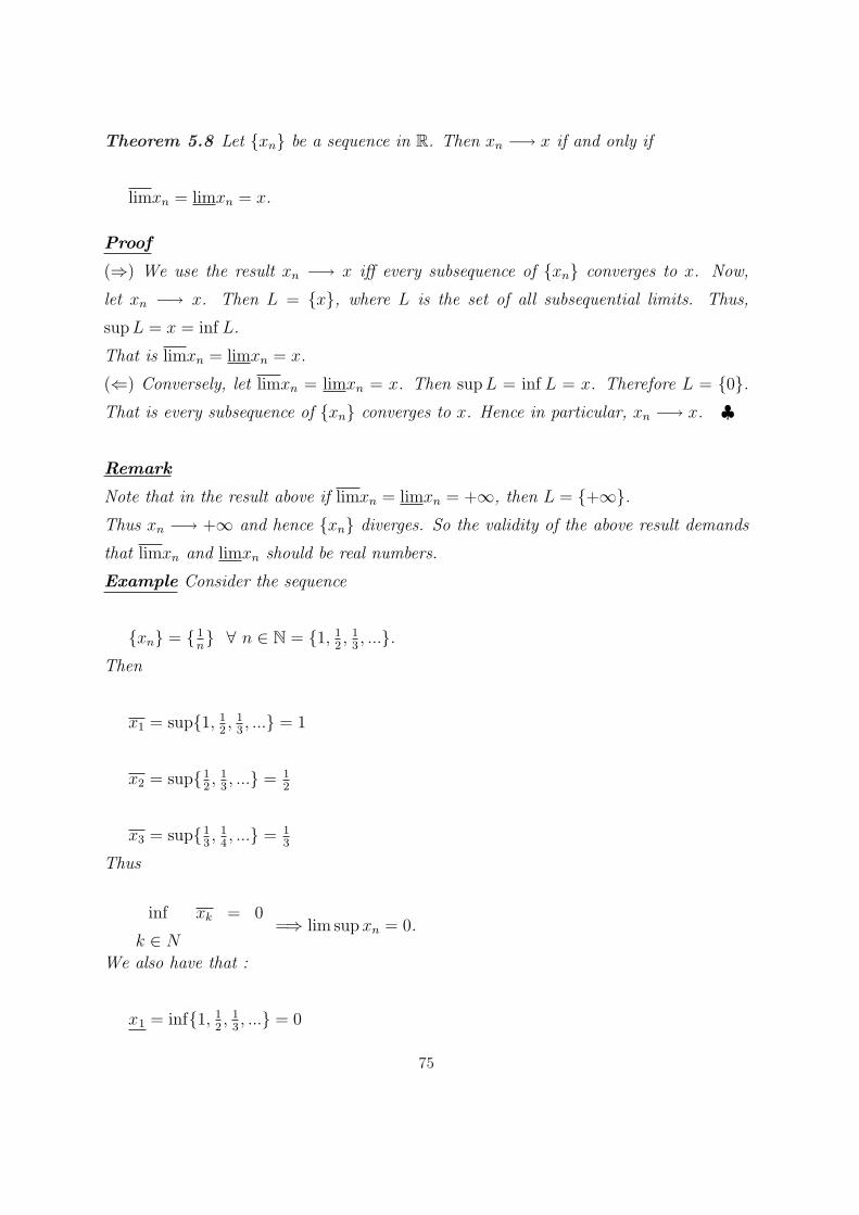
Theorem 5.8 Let xn be a sequence in R. Then xn −→ x if and only if

limxn = limxn = x.

Proof

(⇒) We use the result xn −→ x iff every subsequence of xn converges to x. Now,

let xn −→ x. Then L = x, where L is the set of all subsequential limits. Thus,

sup L = x = inf L.

That is limxn = limxn = x.

(⇐) Conversely, let limxn = limxn = x. Then sup L = inf L = x. Therefore L = 0.That is every subsequence of xn converges to x. Hence in particular, xn −→ x. ♣

Remark

Note that in the result above if limxn = limxn = +∞, then L = +∞.Thus xn −→ +∞ and hence xn diverges. So the validity of the above result demands

that limxn and limxn should be real numbers.

Example Consider the sequence

xn = 1n ∀ n ∈ N = 1, 1

2, 1

3, ....

Then

x1 = sup1, 12, 1

3, ... = 1

x2 = sup12, 1

3, ... = 1

2

x3 = sup13, 1

4, ... = 1

3

Thus

inf xk = 0

k ∈ N=⇒ lim sup xn = 0.

We also have that :

x1 = inf1, 12, 1

3, ... = 0

75

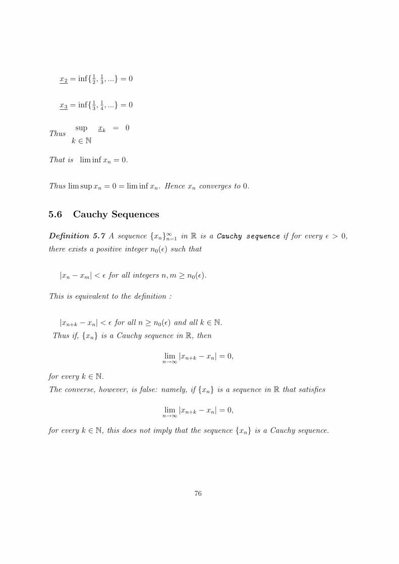
x2 = inf12, 1

3, ... = 0

x3 = inf13, 1

4, ... = 0

Thussup xk = 0

k ∈ N

That is lim inf xn = 0.

Thus lim sup xn = 0 = lim inf xn. Hence xn converges to 0.

5.6 Cauchy Sequences

Definition 5.7 A sequence xn∞n=1 in R is a Cauchy sequence if for every ε > 0,

there exists a positive integer n0(ε) such that

|xn − xm| < ε for all integers n, m ≥ n0(ε).

This is equivalent to the definition :

|xn+k − xn| < ε for all n ≥ n0(ε) and all k ∈ N.

Thus if, xn is a Cauchy sequence in R, then

limn→∞

|xn+k − xn| = 0,

for every k ∈ N.

The converse, however, is false: namely, if xn is a sequence in R that satisfies

limn→∞

|xn+k − xn| = 0,

for every k ∈ N, this does not imply that the sequence xn is a Cauchy sequence.

76

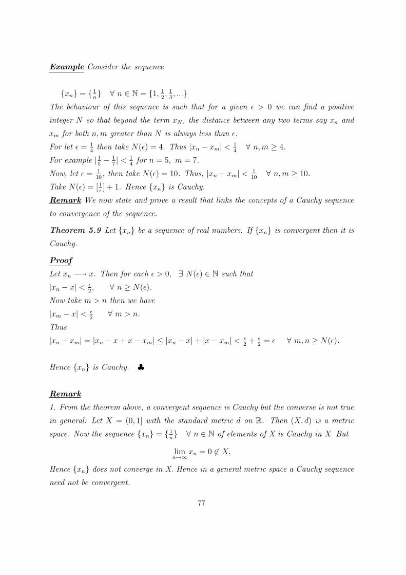
Example Consider the sequence

xn = 1n ∀ n ∈ N = 1, 1

2, 1

3, ...

The behaviour of this sequence is such that for a given ε > 0 we can find a positive

integer N so that beyond the term xN , the distance between any two terms say xn and

xm for both n,m greater than N is always less than ε.

For let ε = 14

then take N(ε) = 4. Thus |xn − xm| < 14

∀ n,m ≥ 4.

For example |15− 1

7| < 1

4for n = 5, m = 7.

Now, let ε = 110

, then take N(ε) = 10. Thus, |xn − xm| < 110

∀ n,m ≥ 10.

Take N(ε) = [1ε] + 1. Hence xn is Cauchy.

Remark We now state and prove a result that links the concepts of a Cauchy sequence

to convergence of the sequence.

Theorem 5.9 Let xn be a sequence of real numbers. If xn is convergent then it is

Cauchy.

Proof

Let xn −→ x. Then for each ε > 0, ∃ N(ε) ∈ N such that

|xn − x| < ε2, ∀ n ≥ N(ε).

Now take m > n then we have

|xm − x| < ε2

∀ m > n.

Thus

|xn − xm| = |xn − x + x− xm| ≤ |xn − x|+ |x− xm| < ε2

+ ε2

= ε ∀ m,n ≥ N(ε).

Hence xn is Cauchy. ♣

Remark

1. From the theorem above, a convergent sequence is Cauchy but the converse is not true

in general: Let X = (0, 1] with the standard metric d on R. Then (X, d) is a metric

space. Now the sequence xn = 1n ∀ n ∈ N of elements of X is Cauchy in X. But

limn→∞

xn = 0 6∈ X,

Hence xn does not converge in X. Hence in a general metric space a Cauchy sequence

need not be convergent.

77

2. A metric space (X, d) is said to be complete if every Cauchy sequence in X converges

to a point in X.

3. Note that R is a complete metric space. Thus every Cauchy sequence in R converges.

Hence for sequences of real numbers, the concept of convergence and the concept of

Cauchy sequence are equivalent.

Theorem 5.10 Every Cauchy sequence is bounded.

Proof

Take ε = 1. By the definition of Cauchy sequence, there exists n0 ∈ N such that

|xn − xm| < 1, ∀ n,m ≥ n0. Therefore, with m = n0,

|xn| ≤ 1 + |xn0| for all n ≥ n0.

Let M = max1 + |xn0|, |x1|, ..., |xn0−1|.Then for all n, |xm| ≤ M.

Thus xn is bounded. ♣

5.7 Solved Problems

1. State the criterion for convergence of a sequence xn of real numbers. Show from

First Principles that the sequence xn = 3 + (−1)n 1n3 : n ∈ N converges to 3.

Solution

Criterion for convergence: Let xn be a sequence in R. Then xn −→ x iff for each

ε > 0, ∃N(ε) ∈ N such that |xn − x| < ε ∀ n ≥ N(ε).

Given the xn above, let ε > 0 be given such that |xn−3| < ε. That is |3+(−1)n1n3−3| < ε

i.e. |(−1)n 1n3 | < ε

i.e. 1n3 < ε

i.e n3 > 1ε

i.e. n > 1

ε13.

Taking N(ε) =[

1

ε13

]+ 1, it follows that |xn − 3| < ε ∀ n ≥ N(ε). Hence xn −→ 3.

2. Give an example of a sequence which is bounded but not convergent.

Solution

78

See examples in notes.

3. (a). Define the concept of a Cauchy sequence.

(b). Prove that a convergent sequence is Cauchy. When is the converse true?

Solution

(a). See notes

(b). The converse is true when the metric space ic complete.

4. Show by induction that the sequence defined by xn+1 =√

2xn ∀n ≥ 2 and x1 =√

2

is monotonic increasing and that xn < 2 ∀ n ∈ N.

State giving reasons whether xn is divergent or convergent in R.

Solution

Left as an exercise.

79

Chapter 6

LIMITS AND CONTINUITY OF

FUNCTIONS IN R

6.1 Introduction

We consider limits and continuity of functions defined on intervals of the real line. Our

aim is to investigate the behavior of a function f(x) when x approaches a given point

which either belongs to the domain of f or it is just a limit point of the domain of f .

6.2 Limit of a Function

The basic idea underlying the concept of the limit of a function f at a point p is to study

the behaviour of f at points close to, but not equal to p.

Definition 6.1 Let E be a subset of R and f : E 7−→ R. Suppose that p is a limit

point of E. The function f has a limit at p if there exists a number L ∈ R such that

given any ε > 0, there exists a δ > 0 for which

|f(x)− L| < ε, for all points x ∈ E satisfying 0 < |x− p| < δ.

80

If this is the case, we write

limx→p

f(x) = L

or f(x) −→ L as x −→ p.

That is, we say f(x) −→ L as x −→ p if for each ε > 0 ∃ δ > 0 such that

0 < |x− p| < δ =⇒ |f(x)− L| < ε.

Remark

1. Note that the point p under consideration being a limit point of E need not belong to

E unless E is a closed interval.

2. Note that we can also view the definition above through the concept of open neighbor-

hoods: We say that

f(x) −→ L as x −→ p if and only if for each open nbhd N(L, ε) of L, there exists

another nbhd N(p, δ) of p such that f(x) ∈ N(L, ε) whenever x ∈ N(p, δ).

Figure 6.1: Limit of a function f

3. In the definition of limit, the choice of δ for a given ε may depend not only on ε and

the function but also on the point p.

81

4. If p is not a limit point of E, then for δ sufficiently small, there do not exist any

x ∈ E so that 0 < |x − p| < δ. Thus, if p is an isolated point of E, the concept of the

limit of a function at p has no meaning.

5. Let E ⊂ R and p a limit point of E. To show that a given function f does not have

a limit at p, we must show that for every L ∈ R, ∃ε > 0 such that for every δ > 0, ‘∃ an

x ∈ E with 0 < |x− p| < δ, for which |f(x)− L| ≥ ε.

Example Let E = x ∈ R : 1 < x < 4. Define f : E 7−→ R by f(x) = x2 + 1.

Consider

limx→4

f(x)

Figure 6.2: Limit of f(x) = x2 + 1 as x → 4

As x −→ 4, f(x) −→ 17.

Thus for each ε > 0, ∃ δ > 0 such that

0 < |x− 4| < δ =⇒ |f(x)− 17| < ε

Equivalently, we can say that for each open nbhd N(17, ε) of the number 17 there exists

another open nbhd N(4, δ) of the number 4 such that f(x) ∈ N(17, ε) whenever x ∈N(4, δ).

82

Note that the number 4 is just a limit point of E which does not belong to E.

6.3 Some results on Limits of Real-valued Functions

Let E ⊆ R and f : E 7−→ R be a function. Let p be a limit point of E. Then

f(x) −→ L as x −→ p if and only if for every sequence xn converging to p we have

the sequence f(x) converging to L.

Corollary 6.1 If a function f has a limit L as x −→ p, then this limit is unique.

Proof

Let f(x) −→ L as x −→ p. Now, if xn is a sequence such that xn −→ p, then

f(xn) −→ q by the theorem above. But the limit of a sequence is unique. Thus we have

that if also f(x) −→ L′ as x −→ p then f(xn) −→ L′ and consequently L = L′.

Hence the limit of f is unique. ♣

Remark The results above provide a link between the concepts of convergence of a se-

quence and limit of a function.

Example Let E = x ∈ R : 1 < x < 4 and f : E 7−→ R be given by f(x) = 2x. Then

limx→2 f(x) = limx→2 2x = 4.

6.3.1 Limit Theorems

Suppose E ⊆ R and f, g : E 7−→ R, and that p is a limit point of E. If

limx→p f(x) = A and limx→p g(x) = B,

then

(a).lim [f(x) + g(x)] = A + B

x → p

(b).lim [f(x)g(x)] = AB

x → p

83

(c).lim [f(x)

g(x)= A

B

x → pprovided B 6= 0.

(d).lim (cf(x)) = c lim f(x) = cA

x → p x → p

6.3.2 Limits at Infinity

Up to this point we have only considered limits of functions at points p ∈ E. We now

extend the definition to include limits at ∞ or −∞.

Definition 6.2 Let f be a real-valued function such that Dom(f)∩ (a,∞) 6= for every

a ∈ R. The function f has a limit at∞ if there exists a number L ∈ R such that given

ε > 0, there exists a real number M for which |f(x)−L| < ε for all x ∈ Dom(f)∩(M,∞).

Figure 6.3: Limit of a function f at ∞

If this is the case, we write

limx→∞

f(x) = L

Similarly, if Dom(f) ∩ (−∞, b) 6= ∅ for every b ∈ R,

84

limx→−∞ f(x) = L iff given ε > 0, there exists a real number M such that

|f(x)− L| < ε for all x ∈ Dom(f) ∩ (−∞,M).

Remark The hypothesis that Dom(f)⋂

(a,∞) 6= ∅ for all a ∈ R is equivalent to saying

that the domain of the function f is not bounded above. If Dom(f) = N, then the above

definition gives the definition for the limit of a sequence.

Example

Consider the function f(x) = sin xx

defined on (0,∞).

Since | sin x| ≤ 1,

|f(x)| ≤ 1x

for all x ∈ (0,∞).

Let ε > 0 be given. Then with M = 1ε, |f(x)| < ε ∀ x ∈ M .

Therefore,

limx→∞

sin x

x= 0.

6.4 Continuous Functions in R

Definition 6.3 Let E be a subset of R and f a real-valued function with domain E.

The function f is continuous at a point p ∈ E, if for every ε > 0, there exists a

δ > 0 such that |f(x)− f(p)| < ε for all x ∈ E with |x− p| < δ.

The function f is continuous on E if and only if f is continuous at every point p ∈ E.

That is, f : E 7−→ R is continuous at p if for each ε > 0, ∃δ > 0 such that

|x− p| < δ =⇒ |f(x)− f(p)| < ε.

The definition can be rephrased as follows:

A function f : E 7−→ R is continuous at p ∈ E iff given ε > 0,∃ δ > 0 such that

f(x) ∈ N(f(p), ε) for all x ∈ N(p, δ) ∩ E.

85

The figure below illustrates this concept.

Figure 6.4: Continuity of a function f

Remarks

1. If p ∈ E is a limit point of E, then f is continuous at p if and only if

limx→p

f(x) = f(p)

2. If p ∈ E is an isolated point, then every function f on E is continuous at p. This

follows from the fact that for an isolated point p ∈ E, ∃ δ > 0 such that N(p, δ)∩E = p.

Examples

1. Let g be defined as

g(x) =

x2−4x−2

, x 6= 2

2, x = 2

At the point p = 2, limx→2 g(x) = 4 6= g(2).

Thus g is not continuous at p = 2.

However, if we redefine g at p = 2 so that g(2) = 4, then this function is now continuous

at p = 2.

86

2. Let f(x) =

0, x ∈ Qx x ∈ QC

Since limx→0 f(x) = 0 = f(0), f is continuous at p = 0.

On the other hand, since limx→p f(x) fails to exist for every p 6= 0, f is discontinuous

at every p ∈ R, p 6= 0.

3. The function f defined by

f(x) =

1, x ∈ Q0, x ∈ QC

is discontinuous at every x ∈ R.

4. Consider f(x) = 1x. This function is continuous at every p ∈ (0,∞). Thus, f is

continuous at (0,∞) but discontinuous at x = 0.

5. Let f be defined by

f(x) =

0, x = 0

x sin 1x, x 6= 0

Then limx→0 f(x) = 0 = f(0)

Thus f is continuous at x = 0.

6. The function f : (0, 1) −→ (0, 1)

f(x) =

0, if x is irrational1n, if x is rational with x = m

nin lowest terms

is discontinuous at every rational number in (0, 1) and continuous at every irrational

number in (0, 1).

87

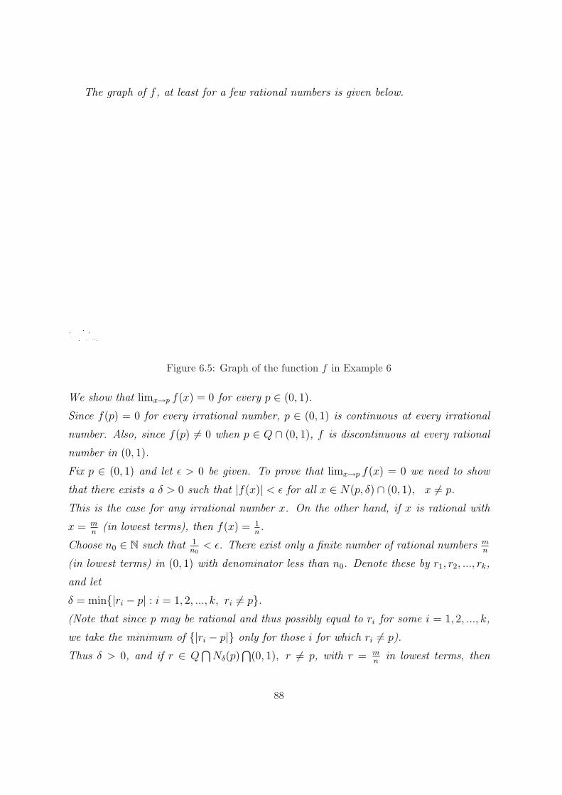
The graph of f , at least for a few rational numbers is given below.

Figure 6.5: Graph of the function f in Example 6

We show that limx→p f(x) = 0 for every p ∈ (0, 1).

Since f(p) = 0 for every irrational number, p ∈ (0, 1) is continuous at every irrational

number. Also, since f(p) 6= 0 when p ∈ Q ∩ (0, 1), f is discontinuous at every rational

number in (0, 1).

Fix p ∈ (0, 1) and let ε > 0 be given. To prove that limx→p f(x) = 0 we need to show

that there exists a δ > 0 such that |f(x)| < ε for all x ∈ N(p, δ) ∩ (0, 1), x 6= p.

This is the case for any irrational number x. On the other hand, if x is rational with

x = mn

(in lowest terms), then f(x) = 1n.

Choose n0 ∈ N such that 1n0

< ε. There exist only a finite number of rational numbers mn

(in lowest terms) in (0, 1) with denominator less than n0. Denote these by r1, r2, ..., rk,

and let

δ = min|ri − p| : i = 1, 2, ..., k, ri 6= p.(Note that since p may be rational and thus possibly equal to ri for some i = 1, 2, ..., k,

we take the minimum of |ri − p| only for those i for which ri 6= p).

Thus δ > 0, and if r ∈ Q⋂

Nδ(p)⋂

(0, 1), r 6= p, with r = mn

in lowest terms, then

88

r ≥ n0. Therefore, |f(r)| = 1n

< ε.

Thus |f(x)| < ε for all x ∈ Nδ(p)⋂

(0, 1), x 6= p. ♣

6.5 Uniform Continuity

Definition 6.4 Let E ⊆ R and f : E 7−→ R be a function. Then f is said to be

uniformly continuous on E if for each ε > 0, ∃ δ > 0(depending on ε) such that for

any pair of points x, y ∈ E we have

|x− y| < δ =⇒ |f(x)− f(y)| < ε.

Remarks

1. Note that δ > 0 depends only on ε but not on the choice of the pair of points x and y.

2. Note that if f is uniformly continuous on E, then it is continuous at every point of

E.

Clearly,

Uniform continuity =⇒ pointwise continuity.

But the converse is not true in general.

Example

1. Let f : R 7−→ R be defined by

f(x) = x2.

Consider the continuity of f at x = p. Let ε > 0 be given such that

|f(x)− f(p)| < ε

i.e, |x2 − p2| < ε

|x− p| < ε|x+p|

i.e. take δ(ε, p) = ε|x+p| .

Here we note that δ > 0 depends not only on ε but also on the point p under considera-

tion. Hence f(x) = x2 is continuous in a pointwise sense(i.e. pointwise continuous) but

not uniformly continuous.

Example Let f : R 7−→ R be defined by f(x) = 2x.

89

Consider continuity at x = p. Let ε > o be given such that:

|f(x)− f(p)| < ε

i.e. |2x− 2p| < ε

2|x− p| < ε

|x− p| < ε2

Take δ(ε) = ε2. Then we have

|x− p| < δ =⇒ |f(x)− f(p)| < ε.

Here δ > 0 depends on only ε but not on the point p under consideration. Hence the

function f(x) = 2x is uniformly continuous.

Theorem 6.2 A continuous real-valued function on a closed and bounded interval [a, b]

is uniformly continuous.

Example

The function f(x) = x2 is continuous on [0,∞) but not uniformly continuous on [0,∞).

On the other hand, the interval (0, 1) is bounded but not closed. The function f(x) = 1x

is continuous on (0, 1) but is not uniformly continuous on (0, 1).

Example Let f : [0, 1] 7−→ R be defined by f(x) = x2. We show that f is uniformly

continuous on [0, 1].

Proof

Let x, y ∈ [0, 1]. Then

|f(x)− f(y)| = |x2 − y2| = |(x + y)(x− y)| = |x + y||x− y|.

Since 0 ≤ x ≤ 1 and 0 ≤ y ≤ 1, we have

x + y ≤ 1 + 1 = 2

Therefore |x + y||x− y| ≤ 2|x− y|.Now, let ε > 0 be given such that

90

|f(x)− f(y)| < ε

i.e. 2|x− y| < ε.

Taking δ(ε) = ε2, it follows that:

|x− y| < δ =⇒ |f(x)− f(y)| < ε.

Hence f(x) = x2 is uniformly continuous on [0, 1].

6.6 Points of Discontinuity of a Function

We now take a closer look at both limits and continuity for real-valued functions defined

on an interval I ⊂ R. More specifically, we will be interested in classifying the types of

discontinuities that such a functions may have.

The concept of discontinuity will play an important role in Riemann integration (which

is the subject of study in the last chapter in this course).

6.6.1 Right and Left Limits

Definition 6.5 Let E ⊂ R and let f be a real-valued function on E. Suppose p is a

limit point of E ∩ (p,∞).

Then f has a right limit at p if there exists a number L ∈ R such that given any

ε > 0,∃ a δ > 0 for which |f(x)− L| < ε for all x ∈ E satisfying p < x < p + δ.

The right limit of f , if it exists, is denoted by

f(p+) =

lim f(x) = lim f(x)

x → p+ x → p

x > p

Similarly, if p is a limit point of E⋂

(−∞, p), the left limit of f at p, if it exists, is

denoted by f(p−), and we write

91

f(p−) =

lim f(x) = lim f(x)

x → p− x → p

x < p

If I is any interval with int(I) 6= ∅, and f : I 7−→ R, then f has a limit at p ∈ int(I) if

and only if

(1). f(p+) and f(p−) both exist, and

(2). f(p+) = f(p−).

Definition 6.6 Let E ⊂ R and let f be a real-valued function on E. The function f

is right continuous(left continuous) at p ∈ E if for any ε > 0,∃ a δ > 0 such that

|f(x)− f(p)| < ε for all x ∈ E with p ≤ x < p + δ (p− δ < x ≤ p)

Theorem 6.3 A function f : (a, b) 7−→ R is right continuous at p ∈ (a, b) if and only

if f(p+) exists and equals f(p).

Similarly, f is left continuous at p iff f(p−) exists and equals f(p).

6.6.2 Types of Discontinuities

By the previous theorem, a function f is continuous at p ∈ (a, b) if and only if

1. f(p+) and f(p−) both exist, and

2. f(p+) = f(p−) = f(p).

A real-valued function f defined on an interval I can fail to be continuous at a point

p ∈ I (the closure of I) for several reasons:

One possibility is that limx→p f(x) exists but either does not equal to f(p), or f is not

defined at p. Such a function can easily be made continuous at p by either defining or

92

redefining f at p as follows:

f(p) =lim f(x)

x → p

For this reason, such a discontinuity is called removable discontinuity.

Example

The function

g(x) =

x2−4x−2

, x 6= 2

2, x = 2

is not continuous at 2, since limx→2 g(x) = 4 6= g(2).

Redefine g such that g(2) = 4, then the resulting function is then continuous at 2.

Example The function f defined on (0,∞) given by f(x) = x sin 1x, is not defined at 0.

If we define f on [0,∞) by

f(x) =

0, x = 0

x sin 1x

x > 0

then f is now continuous at 0.

Another possibility is that f(p+) and f(p−) both exist, but are not equal. This type of

discontinuity is called a jump discontinuity or discontinuity of the first kind or simple

discontinuity.

Definition 6.7 Let f be a real-valued function defined on an interval I. Then f has a

discontinuity of the first kind at p ∈ Int(I) if f(p+) and f(p−) both exist, but

f is discontinuous at p.

93

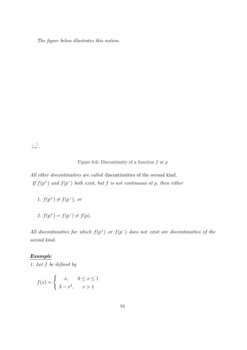
The figure below illustrates this notion.

Figure 6.6: Discontinuity of a function f at p

All other discontinuities are called discontinuities of the second kind.

If f(p+) and f(p−) both exist, but f is not continuous at p, then either

1. f(p+) 6= f(p−), or

2. f(p+) = f(p−) 6= f(p).

All discontinuities for which f(p+) or f(p−) does not exist are discontinuities of the

second kind.

Example

1. Let f be defined by

f(x) =

x, 0 ≤ x ≤ 1

3− x2, x > 1

94

The graph of f is given below:

Figure 6.7: Discontinuity of f at 1

If x < 1, then f(x) = x. Therefore,

f(1−) =lim f(x) = lim x = 1 = f(1)

x → 1− x → 1

f(1+) =lim f(x) = lim (3− x2 = 2

x → 1+ x → 1

Therefore, f(1−) = f(1) = 1, and f(1+) = 2.

Thus, f is left continuous at 1, but not continuous. Since both right and left limits exist

at 1, the function f has a jump discontinuity(discontinuity of the first kind) at 1.

2. Let [x] denote the greatest integer function, i.e. for each x, [x] = largest integer n

that is less than or equal to x.

e.g [2.9] = 2, [3.1] = 3, and [−1.5] = −2.

95

Below is a section of the graph of f .

Figure 6.8: Graph of f(x) = [x]

For all n ∈ N,lim [x] = n− 1

x → n−and

lim [x] = n

x → n+

Thus f has a discontinuity of the first kind at each n ∈ N.

6.7 Solved Problems

1. Give the definition of a limit of a function and prove that this limit is unique.

Solution

Let E ⊆ R and f : E 7−→ R be a function. Let p be a limit point of E. We say that

f(x) −→ L as x −→ p if for each ε > 0, ∃ δ > 0 such that

|f(x)− L| < ε whenever 0 < |x− p| < δ.

We show that L is unique. Suppose f(x) −→ L and also f(x) −→ L′ as x −→ p, L 6= L′.

96

Then for a sequence xn −→ p we have that:

f(xn) −→ L and f(xn) −→ L′. But limit of a sequence is unique. Hence L = L′.

Hence the limit of f (if it exists) is unique. ♣

2. Given f(x) = x2 − 5x, show that limx→2 f(x) = −6. Determine a value for δ > 0

associated with ε > 0 in accordance with the definition of limit of a function.

Solution

f(x) = x2 − 5x.

lim f(x)

x → 2= 22 − 5(2) = 4− 10 = −6.

Now, let ε > 0 be given and suppose that

|f(x)− (−6)| < ε whenever 0 < |x− 2| < δ

|x2 − 5x + 6| = |(x− 2)(x− 3)| =

Take δ = 1 so that 0 < |x− 2| < 1. Then we have

x− 2 < 1 =⇒ x < 1 + 2 = 3.

Also

−(x− 2) < 1 =⇒ −x + 2 < 1 =⇒ −x < 1− 2 = −1 > 1.

That is 1 < x < 3. But for 1, x < 3, we have |x− 3| < 2.

Thus

|x2 − 5x + 6| = |x− 3||x− 2| < 2|x− 2| whenever 0 < |x− 2| < 1.

97

Take δ = ε2. Then

0 < |x− 2| < δ = ε2

=⇒ |x− 3||x− 2| < 2. ε2

= ε

=⇒ |(x2 − 5x− (−6)| < ε =⇒ |f(x)− (−6)| < ε.

Thus ε = 12

and δ = 14

will do.

3.(a). Define the concept of uniform continuity.

(b). Let f : R 7−→ R be defined by f(x) = |x|, ∀ x ∈ R.

Show that f is uniformly continuous on R.

Solution

f : E 7−→ R is uniformly continuous on E if for each ε > 0, ∃ δ > 0(depending on ε)

such that for any pair of points x, y ∈ E we have

|x− y| < δ =⇒ |f(x)− f(y)| < ε.

Given f(x) = |x|, let ε > 0 be given such that |f(x)− f(y)| < ε

i.e.∣∣∣|x| − |y|

∣∣∣ < ε.

But∣∣∣|x| − |y|

∣∣∣ < |x− y|.

Thus taking δ(ε) = ε, we have

|x− y| < δ = ε =⇒∣∣∣|x| − |y|

∣∣∣ < ε.

Hence f(x) = |x| is uniformly continuous.

4. Let f : R 7−→ R be defined by

98

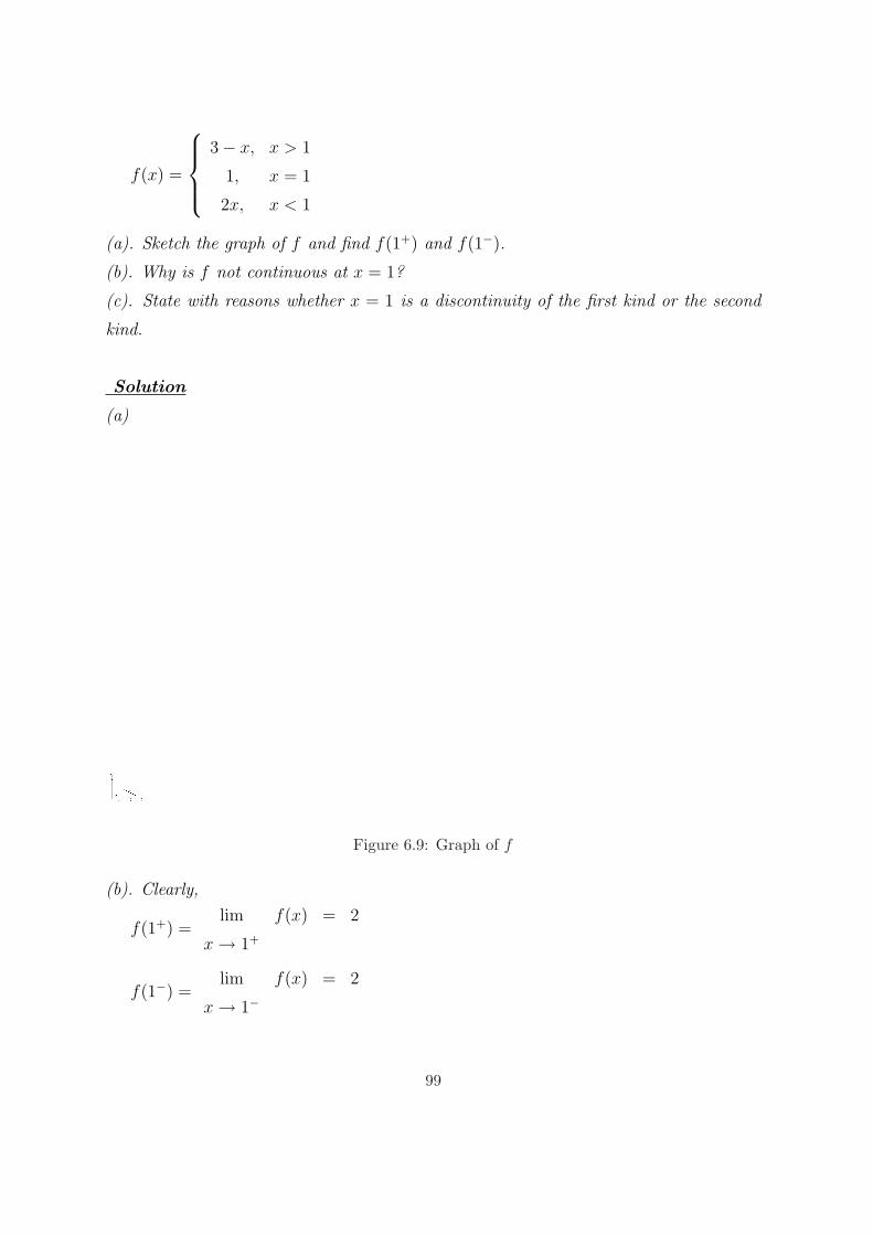
f(x) =

3− x, x > 1

1, x = 1

2x, x < 1

(a). Sketch the graph of f and find f(1+) and f(1−).

(b). Why is f not continuous at x = 1?

(c). State with reasons whether x = 1 is a discontinuity of the first kind or the second

kind.

Solution

(a)

Figure 6.9: Graph of f

(b). Clearly,

f(1+) =lim f(x) = 2

x → 1+

f(1−) =lim f(x) = 2

x → 1−

99

Therefore f(1+) = f(1−).

That islim f(x) = 2

x → 1.

But f(1) = 1 6= 2 =lim f(x)

x → 1

(c). Using (b) and the fact that f(1+) and f(1−) both exist, it follows that x = 1 is a

discontinuity of the first kind.

100

Chapter 7

PROPERTIES OF CONTINUOUS

FUNCTIONS IN R

7.1 Introduction

Functions that are continuous on intervals have a number of very important properties

that are not possessed by general continuous functions.

Definition 7.1 A function f : A 7−→ R is said to be bounded on A if there exists a

constant M > 0 such that |f(x)| ≤ M for all x ∈ A.

(*)

That is a function is bounded on a set if its range is a bounded set in R.

A function f is unbounded on a given set if there is no particular number M with the

property (*) or if given any M > 0, there exists a point xM ∈ A such that |f(xM)| > M .

Examples

Let A = (0,∞) and f : (0,∞) 7−→ R be given by f(x) = 1x. Then f is not bounded on A

because for any M > 0 we can take the point xM = 1M+1

in A to get

f(xM) = 1xM

= M + 1 > M .

Remark This example shows that continuous functions need not be bounded.

101

7.2 Boundedness Theorem

Theorem 7.1 (Boundedness Theorem) Let I = [a, b] be a closed bounded interval

and let f : I 7−→ R be continuous on I. Then f is bounded on I.

7.3 Location of Roots Theorem

Theorem 7.2 (Location of Roots Theorem) Let I = [a, b] and let f : I 7−→ R be

continuous on I. If f(a) < 0 < f(b), or if f(a) > 0 > f(b), then there exists a number

c ∈ (a, b) such that f(c) = 0.

Proof

For definiteness, let f(a) < 0 and f(b) > 0. Let A = x : f(x) < 0, for all x ∈ [a, b].

Then A is a set of real numbers bounded above by b. Thus b is an upper bound.

By the Completeness Property, A has the least upper bound, say x0.

Clearly, a < x0 < b. We now show that f(x0) = 0.

Suppose f(x0) < 0. Since f is continuous at x0, ∃ δ > 0 such that f(x0) < 0 for

x0 − δ < x < x0 + δ.

Thus f(x0 < 0 in (x0, x0 + δ). But this contradicts the definition of x0 as the least upper

bound of A. Hence the assumption that f(x0) < 0 is incorrect. Thus f(x0) 6< 0.

Now assume f(x0) > 0. Then there exists δ′> 0 such that f(x) > 0 ∀ x ∈ (x0−δ

′, x0).

This again contradicts the definition of x0 as the least upper bound of A. Thus f(x0) 6> 0.

Hence f(x0) = 0.

Hence taking c = x0, we have c ∈ (a, b) such that f(c) = 0. ♣

102

The figure below illustrates this concept.

Figure 7.1: Location of Roots

Remark

The point c is where the graph of f crosses the x-axis. If f has turning points between

a and b then we may have more than one such a number c.

Example The function f(x) = xex − 2 has a root c in the interval [0, 1] because f is

continuous on [0, 1] and f(0) = −2 < 0 and f(1) = e− 2 > 0.

Remark The next result is a generalization of the Location of Roots Theorem. It assures

us that a continuous function on an interval takes on (at least once) any number that

lies between two of its values.

7.4 Bolzano’s Intermediate Value Theorem (IVT)

Theorem 7.3 (Bolzano’s Intermediate Value Theorem (IVT) Let f : [a, b] 7−→R be a continuous function. Let f(a) 6= f(b) and f(a) < c < f(b). Then there exists at

least one number x0 ∈ (a, b) such that f(x0) = c.

103

The figure below illustrates this concept.

Figure 7.2: IVT

Proof

For x ∈ [a, b], define a function by

g(x) = c− f(x), c a constant.

Now without loss of generality(WLOG), assume f(a) < f(b). That is

f(a) < c < f(b).

Thus

g(a) = c− f(a) > 0

g(b) = c− f(b) < 0

104

Since f is continuous and c is a constant it follows that g is also continuous on [a, b]. Now

g(a) > 0 and g(b) < 0 =⇒ that ∃ x0 ∈ (a, b) such that g(x0) = 0

i.e. c− f(x0) = 0

i.e. f(x0) = c ♣Remark Note that the IVT simply asserts that a continuous function on a closed interval

assumes its intermediate value.

7.4.1 Applications of the IVT ( Existence and location of real roots of poly-

nomial equations)

Example 1 Use the IVT to show that the equation x3 − 4x = 0 has at least one real

root between −3 and −1.

Solution

Consider the function f : [−3,−1] 7−→ R defined by f(x) = x3 − 4x.

Then f is continuous on [−3,−1] and that

f(−3) = −15 < 0

f(−1) = 3 > 0

Let c = 0. Then f(−3) < 0 < f(−1).

Hence by the IVT, ∃ x0 ∈ (−3,−1) such that f(x0) = c = 0.

Hence the equation x3 − 4x = 0 has a real root between −3 and −1.

Example 2 Use the IVT to show that the equation e2−3x − e−x = 0 has a real root

between 0 and 3. Find this root.

Solution

Consider the function f : [0, 3] 7−→ R defined by f(x) = e2−3x − e−x. Then f is continu-

105

ous on [0, 3], and

f(0) = e2 − 1 > 0

f(3) = e2−9 − e−3 = e−7 − e−3 = 1e7 − 1

e3 < 0.

Now take c = 0. Then we have that f(3) < 0 < f(0). By the IVT, there exists x0 ∈ (0, 3)

such that f(x0) = 0.

Hence the equation e2−3x − e−x = 0 has a real root between 0 and 3.

Now, given e2−3x − e−x = 0 =⇒ e2−3x = e−x =⇒=⇒ ln e2−3x = ln e−x

or 2− 3x = −x

or x = 1.

7.5 Solved Problems

1. State and prove the IVT.

Solution Let f : [a, b] 7−→ R be continuous with f(a) 6= f(b 6=). Let c be a constant

between f(a) and f(b). Then there exists x0 ∈ (a, b) such that f(x0) = c.

Proof (Bookwork !)

2. Let f : [π4, π] 7−→ R be defined by f(x) = sin x− 2

πx. Show that there exists α ∈ (π

4, π)

such that sin α = 2πα.

Find the non-zero value of α.

Solution

Note that f is continuous on [π4, π].

f(π4) = sin(π

4)− 2

π(π

4) = 1√

2− 1

2> 0

f(π) = sin π − 2ππ = 0− 2 = −2 < 0.

Thus f(π) < 0 < f(Π4).

Let c = 0. Then by the IVT, there exists α ∈ (π4, π) such that f(α) = 0.

106

sin α− 2πα = 0

i.e. sin α = 2πα

Now draw the graphs of y = sin x for 0 ≤ x ≤ π and y = 2πx on the same axes. Their

point of intersection is the value of α.

Figure 7.3: Graphs of sin(x) and 2πx

From the figure above,

α =π

2.

107

Chapter 8

THE RIEMANN INTEGRAL

8.1 Introduction

We study the formulation of the Riemann integral and its properties and classify func-

tions as Riemann integrable or not.

8.2 Partitions of an Interval

Let [a, b] be an interval in R and let x0, x1, ..., xn be such that:

a = x0 < x1 < ... < xn = b

Then the set

P = x0, x1, ..., xn

is called a partition of [a, b].

Remarks

1. Note that on a given interval we can define an infinite number of partitions.

2. The class of all partitions of an interval [a, b] is usually denoted by P[a, b]. Thus

P ∈ P[a, b] means P is a partition of [a, b].

108

Example Let [a, b] = [0, 10] be a given interval in R. Then we have

P1 = 0, 2, 4, 6, 8, 10 is a partition of [0, 10].

Figure 8.1: Partition P1

Also

P2 = 0, 1, 2, 3, 4, 5, 6, 7, 8, 9, 10 is a partition of [0, 10].

109

The figure below shows partition P2.

Figure 8.2: Partition P2

Also

P3 = 0, 3, 7, 10 is a partition of [0, 10].

110

The figure below shows partition P3.

Figure 8.3: Partition P3

Definition 8.1 Let P be a partition of a given interval [a, b]. Then the number denoted

by µ(P ) and given by

µ(P ) = max1≤i≤n

|xi − xi−1|

is called the mesh or norm of the partition P .

Definition 8.2 Let P1, P2 ∈ P[a, b]. Then P1 is said to be finer than P2, or equiva-

lently, P2 is coarser than P1 if every point of P2 is a point of P1.

Remark

P2 is finer than P3 in the above examples of partitions.

Definition 8.3 Let P1, P2 ∈ P[a, b]. P = P1 ∪ P2 is called a common refinement of

P1 and P2.

In the example above, the common refinement of P1 and P2 is P = P1∪P2 = 0, 1, 2, 3, 4, 5, 6, 7, 8, 9, 10.

111

8.3 Lower and Upper Riemann Sums

Let f be a bounded real-valued function on [a, b]. Given a partition P ∈ P[a, b]

P = a = x0, x1, x2, ..., xn = b of [a, b] for each i = 1, 2, ..., n,

Let 4xi = xi − xi−1,

mi = inff(x) : xi−1 ≤ x ≤ xi,

Mi = supf(x) : xi−1 ≤ x ≤ xi

Since f is bounded, by the least upper bound property the quantities mi and Mi exist in R.

M = supf(x) : a ≤ x ≤ b

m = inff(x) : a ≤ x ≤ b

Clearly m ≤ mi ≤ Mi ≤ M ∀ i = 1, 1, 2, ..., n.

The Upper Riemann Sum U(P, f) for the partition P and function f is defined by

U(P, f) =

n∑

Mi 4 xi

i = 1

Similarly, the Lower Riemann Sum L(P, f) is defined by

L(P, f) =

n∑

mi 4 xi

i = 1

Since mi ≤ Mi, for all i = 1, 2, ..., n , we always have

L(P, f) ≤ U(P, f).

112

It follows that since m ≤ mi ≤ Mi ≤ M ∀ i = 1, 2, ..., n,

m

n∑ 4xi

i = 1

≤n∑

mi 4 xi

i = 1

≤n∑

Mi 4 xi

i = 1

≤ M

n∑ 4xi

i = 1

Now

n∑ 4xi

i = 1

= xn − x0 = b− a

Thus

m(b− a) ≤ U(P, f) ≤ M(b− a) and

m(b− a) ≤ L(P, f) ≤ M(b− a), ∀ P ∈ P[a, b].

Figure 8.4: Upper Sum U(P, f)

113

The figure below shows L(P, f).

Figure 8.5: Lower Sum L(P, f)

U(P, f) represents the circumscribed rectangular approximation to the area under the

graph of f . Similarly, the lower sum represents the inscribed rectangular approximation

to the area under the graph of f .

8.4 Upper and Lower Riemann Integrals

Definition 8.4 Let f be a bounded real-valued function on the closed and bounded in-

terval [a, b]. The upper and lower integrals of f , denoted,

∫ b

af and

∫ b

af , respectively, are defined by

∫ b

af = infU(P, f) : P is a partition of [a, b]

∫ b

af = supL(P, f) : P is a partition of [a, b]

114

Since the sets U(P, f) and L(P, f) are nonempty and bounded, the lower and upper

Riemann integrals of a bounded function f : [a, b] 7−→ R always exist.

Theorem 8.1 Let f be a bounded real-valued function on [a, b]. Then

∫ b

a

f ≤∫ b

a

f

Proof

Given any two partitions P1 and P2 of [a, b],

L(P1, f) ≤ L(P1 ∪ P2, f) ≤ U(P1 ∪ P2) ≤ U(P2, f).

Thus

L(P1, f) ≤ U(P2, f) for any partitions P1 and P2.

Hence

∫ b

a

f = supP

L(P1, f) ≤ U(P2, f),

for any partition.

Taking the infimum over P2 gives the result. ♣

8.5 The Riemann Integral

If f : [a, b] 7−→ R is bounded, then the lower and upper integrals of f on [a, b] always

exist and satisfy ∫ b

a

f ≤∫ b

a

f

115

Remark

There is a large family of functions for which equality holds; such functions are said to

be integrable.

8.5.1 Criterion for Riemann Integrability

Definition 8.5 Let f be a bounded real-valued function on the closed and bounded

interval [a, b]. If

∫ b

a

f =

∫ b

a

f

then f is said to be Riemann integrable or integrable on [a, b]. The common value

is denoted by

∫ b

af or

∫ b

af(x) and is called the Riemann integral or integral of f over [a, b].

Theorem 8.2 Let f be bounded on [a, b]. Then f is Riemann integrable if and only if

for each ε > 0 ∃ P ∈ P[a, b] such that

U(P, f)− L(P, f) < ε.

Proof

(=⇒) Let f be Riemann integrable over [a, b]. Then

∫ b

a

fdx =

∫ b

a

fdx =

∫ b

a

fdx

But

∫ b

afdx = inf

U(P, f) : P ∈ P[a, b]

∫ b

afdx = sup

L(P, f) : P ∈ P[a, b]

Therefore, given any ε > 0, ∃ P1, P2 ∈ P[a, b] such that

116

U(P1, f) <∫ b

afdx + ε

2=

∫ b

afdx + ε

2

and

L(P2, f) >∫ b

afdx− ε

2=

∫ b

af − ε

2.

Now, let P = P1 ∪ P2. Therefore P1 ⊆ P and P2 ⊆ P .

Hence

U(P, f) <

∫ b

a

fdx +ε

2

and

L(P, f) >

∫ b

a

fdx− ε

2

Thus ∫ b

a

fdx− ε

2< L(P, f) < U(P, f) <

∫ b

a

fdx +ε

2

That is

U(P, f)− L(P, f) <( ∫ b

a

fdx +ε

2

)−

( ∫ b

a

fdx− ε

2

)<

∫ b

a

fdx +ε

2−

∫ b

a

fdx +ε

2= ε.

That is

U(P, f)− L(P, f) < ε.

(⇐=) Conversely, for each ε > 0, let P ∈ P[a, b] such that

U(P, f)− L(P, f) < ε.

Then we have

U(P, f) ≥∫ b

a

fdx ≥∫ b

a

fdx ≥ L(P, f).

Therefore ∫ b

a

fdx−∫ b

a

fdx = U(P, f)− L(P, f) < ε, ∀ ε > 0.

Since ε > 0 is arbitrary, we have that

117

∫ b

a

fdx =

∫ b

a

fdx =

∫ b

a

fdx.

Hence f is Riemann integrable. ♣

8.5.2 Some Classes of Riemann Integrable Functions

Theorem 8.3 Let f be a bounded function on [a, b]. If f is monotonic on [a, b], then it

is integrable.

Figure 8.6: Bounded and monotonic function f

Proof

Without loss of generality(WLOG), assume f is monotonic increasing. The case when

f is monotonic decreasing can be proved similarly.

Let P be a partition of [a, b] and µ(P ) be the mesh of P . Then since f is monotonic

increasing, we have

118

Mi = f(xi) and mi = f(xi−1)

Thus

U(P, f)− L(P, f) =

n∑

Mi 4 xi

i = 1

−n∑

mi 4 xi

i = 1

=

n∑

(Mi −mi)4 xi

i = 1

=

n∑ (

f(xi)− f(xi−1))4 xi

i = 1

≤ µ(P )

n∑ (

f(xi)− f(xi−1))

i = 1

= µ(P )(f(b)− f(a)

)

But for each ε > 0, P can be chosen so that

µ(P ) <ε

f(b)− f(a)

Hence we have

U(P, f)− L(P, f) < µ(P )(f(b)− f(a)

)<

ε(f(b)− f(a)

)

f(b)− f(a)= ε

That is

U(P, f)− L(P, f) < ε

Hence f is Riemann integrable. ♣

Theorem 8.4 Let f be a bounded function on [a, b]. If f is continuous then f is Rie-

mann integrable.

Proof

Let f : [a, b] 7−→ R be continuous. Since f acts on a closed and bounded set (and hence a

119

compact set), then f is uniformly continuous. Thus given ε > 0 we can choose a number

η such that η(b− a) < ε. Then ∃ δ > 0 such that for any pair of points x and x′,

|x− x′| < δ =⇒ |f(x)− f(x′)| < η

We also have

|xi − xi−1| < δ =⇒ |f(xi)− f(xi−1)| < η

(*)

Choosing a partition P of [a, b] such that µ(P ) < δ,

Mi = f(xi), mi = f(xi−1), we have µ(P ) < δ =⇒ Mi −mi < η by (*).

Thus

U(P, f)− L(P, f) =

n∑

Mi 4 xi

i = 1

−n∑

mi 4 xi

i = 1

=

n∑

(Mi −mi)4 xi

i = 1

<

n∑

η4 xi

i = 1

= η

n∑ 4xi

i = 1

= η(b− a) < ε

Hence f is Riemann integrable.

Example

Consider the function

f : [0, π2] 7−→ R defined by f(x) = sin2 x .

120

We note that f is continuous on [0, π2] and hence it is Riemann integrable on [0, π

2].

Indeed

∫ π2

0

sin2 xdx =

∫ π2

0

(1

2− 1

2cos2 x)dx

=1

2x− 1

4sin 2x

∣∣∣π2

0

=π

4− 1

4sin Π =

1

4

Theorem 8.5 Let f and g be Riemann integrable functions and c be a constant. Then

the following functions are also integrable:

(1). f + g

(2). cf

Definition 8.6 Let f be a bounded function on [a, b]. Then we define the functions f+

and f− as follows:

f+ = maxf(x), 0, ∀ x ∈ [a, b]

f− = max−f(x), 0, ∀ x ∈ [a, b]

We have

f = f+ − f−

and

|f | = f+ + f−

Theorem 8.6 Let f be a bounded function on [a, b]. If f is Riemann integrable then

|f | is also Riemann integrable.

121

Proof

Since f is integrable, for each ε > 0, ∃ P ∈ P[a, b] such that U(P, f)− L(P, f) < ε.

For this partition P ∈ P[a, b] we have M+i = Mi and M+

i ≥ mi,

where M+i = supf+(x) : xi−1 ≤ x ≤ xi .

Hence U(P, f+) = U(P, f) and L(P, f+) ≥ L(P, f)

Thus U(P, f+)− L(P, f+) ≤ U(P, f)− L(P, f) < ε.

Hence f+ is also integrable. But f− = f+ − f is also integrable.

Hence |f | is integrable.

Moreover,

f ≤ |f | =⇒∫

fdx ≤∫|f |dx

Also

−f ≤ |f | =⇒ −∫

fdx ≤∫|f |dx

That is ∣∣∣∫

fdx∣∣∣ ≤

∫|f |dx

8.6 Integral as a Limit

If f is a bounded function on [a, b] and P is any partition of [a, b], then as P is made

finer, the lower sums increase towards the actual integral and the upper sums decrease

towards the actual integral. In this case, we define the Riemann integral as follows:

Definition 8.7 Let f be bounded on [a, b] and P be a partition of [a, b]. Let S(P, f)

denote an arbitrary Riemann sum which is either upper or lower. Then we have

∫ b

a

fdx = limµ(P )→0

S(P, f)

122

Remarks Note that if the partition P is chosen to have n subintervals so that µ(P ) is

expressed in terms of n then we have

∫ b

a

fdx = limn→∞

S(P, f)

Example

Let f : [0, 1] 7−→ R be a bounded function on [0, 1]. Let

P =

0, 1n, 2

n, ..., k

n, ..., n

n= 1

For this partition we can assume, without loss of generality(WLOG), that f is mono-

tonic increasing or monotonic decreasing on the kth subinterval [xk−1, xk].

Mk = sup

f(x) : xk−1 ≤ x ≤ xk

= f(xk) = f( k

n)

or

mk = inf

f(x) : xk−1 ≤ x ≤ xk

= f(xk) = f( k

n)

Hence

S(P, f) =

n∑

Mk 4 xk

k = 1

=

n∑

f( kn)4 xk

k = 1

where 4 xk = xk − xk−1, k = 1, 2, ..., n

Thus ∫ 1

0

fdx = limn→∞

( n∑

k=1

f(k

n)4 xk

)

For this particular partition , we have

µ(P ) =k

n− k − 1

n=

1

n= 4xk

123

Hence

∫ 1

0

fdx = limn→∞

( 1

n

n∑

k=1

f(k

n))

Example

Let f : [0, a] 7−→ R be defined by f(x) = x. Show that

∫ a

0

fdx = limn→∞

(a2

n2

n∑

k=1

k)

Solution

Let P =

0, an, 2a

n, ..., ka

n, ..., a

Then

4xk =ka

n− (k − 1)a

n=

a

n

and

f(ka

n) =

ka

n

Therefore,

S(P, f) =n∑

k=1

f(ka

n)xk

=n∑

k=1

f(ka

n).

a

n

=a2

n2

n∑

k=1

k

Therefore

∫ a

0

fdx = limn→∞

(a2

n2

n∑

k=1

k)

124

Remark In the Riemann approach to integration, one defines the integral of a bounded

real-valued function f as the limit of the Riemann sums of f .

8.7 Solved Problems

1. Let f : [a, b] 7−→ R be a bounded function. Give definitions of lower and upper Rie-

mann sums of f . Explain what is meant by saying that f is Riemann integrable over [a, b].

Solution

(Bookwork!)

2. Show that the function f defined by

f(x) =

1 if x is rational

−1 if x is irrational

is not Riemann integrable.

Solution

Let f be defined as above. Then we have:

Mi = lub

f(x) : x ∈ [xi−1 − xi]

= 1

mi = glb

f(x) : x ∈ [xi−1 − xi]

= −1

Therefore

U(P, f) =n∑

i=1

Mi 4 xi =n∑

i=1

4xi = b− a > 0

L(P, f) =n∑

i=1

mi 4 xi = −n∑

i=1

4xi = −(b− a) < 0

Hence

125

∫ b

a

fdx = glb

U(P, f) : P ∈ P[a, b]

= b− a > 0

and ∫ b

a

fdx = lub

L(P, f) : P ∈ P[a, b]

= 0

Thus ∫ b

a

fdx = −(b− a) < 0 6=∫ b

a

fdx = (b− a) > 0

Hence f is not Riemann integrable.

3. Consider the function f(x) = x3 on [0, a]. Show that

∫ a

0

x3 dx = limn→∞

(a4

n4

n∑

k=1

k3)

Solution

Given f : [0, a] 7−→ R defined by f(x) = x3

Let P ∈ P[0, a] be such that P = 0, an, 2a

n, ..., ka

n, na

n= a

Then

4xk = kan− (k−1)a

n= a

n

f(kan

) = (kan

)3 = a3k3

n3

Therefore ∫ a

0

fdx = limn→∞

( n∑

k=1

a3k3

n3.a

n

)= lim

n→∞

(a4

n4

n∑

k=1

k3)

126

4. Show that g(x) = |x| is Riemann integrable over [−2, 2]. Hence evaluate∫ 2

−2|x| dx.

Solution

Given g as above, let f(x) = x, ∀ x ∈ [−2, 2]. Then f is Riemann integrable over

[−2, 2] since it is continuous. Thus,

|f | = |f(x)| = |x| = g(x)

is also integrable over [−2, 2].

Now |f | = f+ + f−

Therefore g(x) = |x| =

x x > 0

−x x < 0

Therefore∫ 2

−2|x|dx =

∫ 0

−2−x dx +

∫ 2

0x dx =

[−x2

2

]0

−2+

[x2

2

]2

0= 4.

5. The following is a Riemann sum

π

n

n∑

k=1

sink

nπ

Use the fact to evaluate

limn→∞

(π

n

n∑

k=1

sink

nπ)

Solution

Consider a function f : [0, π] 7−→ R defined by f(x) = sin x.

Let P be a partition of [0, π] such that

P = 0, πn, 2π

n, ..., kπ

n, ..., π

Then 4xk = kπn− (k−1)π

n= π

n

127

∴ f(xk) = f(kπn

) = sin kπn

Therefore ∫ π

0

fdx = limn→∞

( n∑

k=1

sinkπ

n.π

n

)= lim

n→∞

(π

n

n∑

k=1

sinkπ

n

)

Thus

limn→∞

(π

n

n∑

k=1

sinkπ

n.π

n

)=

∫ π

0

sin xdx =[− cos x

]π

0= − cos π + cos 0 = 1 + 1 = 2.

128

Bibliography

[1] White, A.J, Real Analysis: an introduction, Addison-Wesley, London, Great

Britain, 1968.

[2] Bartle, Robert G., and Sherbert, Donald R., Introduction to Real Analysis,

Third Edition, John Wiley Sons, New York, 2000.

[3] Rudin, Walter, Principles of Mathematical Analysis, Third Edition, McGraw-

Hill, New York, 1976.

[4] Royden, H.L, Real Analysis, Third Edition, Prentice-Hall, New Jersey, 1988.

[5] Stoll, Manfred, Introduction to Real Analysis, Second Edition, Addison-

Wesley,Boston, 2001.

129

Index

1-to-1 correspondence, 29

Accumulation point, 59

Addition axioms, 6

Aleph nought, 43

Aleph null, 43

Aleph zero, 43

Algebraic number, 47

Algebraic properties, 5

Approximation, 147

Archimedean Property of R, 15

Arithmetic mean, 22

Arithmetic-Geometric Mean Inequality, 22

Bernoulli’s Inequality, 27

Bijection, 29

Bijective mapping, 30

Bolzano’s Intermediate Value Theorem (IVT),

133

Bolzano-Weierstrass Theorem, 88

Boundary of a set, 57

Boundary point, 57

Bounded above, 71

Bounded below, 71

Bounded intervals, 39

Bounded sequence, 85

Bounded set, 71

Boundedness Theorem, 130

Cancellation laws for addition, 10

Cancellation laws for multiplication, 10

Cardinality, 29

Cauchy, 98

Cauchy sequence, 98

Closed interval, 40

Closed set, 60

Closure of a set, 61

Cluster point, 59

Coarser, 144

Common refinement, 144

Commutative group, 9

Completeness Property of R, 76

continuous, 109

Continuous function, 109

Convergence, 81

Convergence of a sequence, 82

Countable set, 30

countable set, 30

Countably infinite, 30

Criterion of convergence, 82

Dense set, 61

Dense subset, 15

Denumerable, 31

130

Discontinuities of the second kind, 121

Discontinuity, 118

Discontinuity of the first kind, 120

Discrete metric, 53

diverge, 82

Divergence, 82

Empty set, 30

Equinumerous, 29

Equivalent, 29

Euclidean space, 55

Even, 14

Familiar metric, 52

Field axioms, 6

Finer, 144

finite set, 30

First Principles, 84

Function, 103

Geometric mean, 22

Greatest integer function, 123

Greatest lower bound, 75

Greatest Lower Bound Property of R, 76

Half-closed, 40

Half-open, 40

Infimum, 72

Infinite sequence, 38

Infinite set, 30

Integers, 4

integrable, 150

Integral as a limit, 158

Interior of a set, 57

Interior point, 56

Intersection of sets, 62

Intervals on R, 39

Irrational numbers, 5

Isolated point, 59

Jump discontinuity, 120

Law of Trichotomy, 9

Least upper bound, 71, 75

Leat Upper Bound Property of R, 76

Left continuous, 119

Left limit, 118

Limit inferior, 93

Limit Infimum, 93

Limit of a sequence, 91

Limit of function, 103

Limit of Riemann sums, 161

Limit superior, 93

Limit supremum, 93

Limit theorems, 107

Limits at infinity, 108

Linit point, 59

Location of Roots Theorem, 130

Lower bound, 71

Lower Riemann integral, 147

Lower Riemann sum, 144

Mathematical induction, 20

Maximum element, 76

Mesh, 143

Metric, 50

131

Metric space, 52

Minimum element, 76

Monotonic, 92

Monotonic decreasing, 92

Monotonic increasing, 92

Monotonic sequence, 91

Multiplication axioms, 9

Natural numbers, 2

Negative, 18

Neighborhood of a point, 55

Nested Interval Property, 41

Nested intervals, 41

No divisors of zero, 10

Nonnegative, 18

Norm, 143

Odd, 14

One-to-one function, 29

Onto function, 29

Open disc, 55

Open interval, 40

Open neighborhood, 55

Open set, 57

Open sphere, 55

Ordered field, 8

Partial ordering, 8

Partition, 140

Partitions of an interval, 139

Point-wise continuity , 115

Points of discontinuity of a function, 118

Polynomial, 46

Polynomial equations, 135

Polynomial of degree n, 46

Positive, 18

Positive real numbers, 18

Properties of integers, 14

Properties of Irrationals, 15

Properties of Positive Real Numbers, 18

Properties of Rationals, 15

Rational numbers, 4

Real line, 2

Real Number System, 5

Real Numbers, 5

Relative metric, 54

Relatively closed set, 64

Relatively open set, 64

Removable discontinuity, 120

Riemann approach to integration, 161

Riemann integrability, 139

Riemann integrable function, 139

Riemann integral, 139, 149

Right continuous, 119

Right limit, 118

Ring, 9

Sequence, 80

Simple discontinuity, 120

Singleton sets, 44

Standard metric, 52

Strictly negative, 18

Strictly positive, 18

Subsequence, 88

Subsequential limit, 88

132

Subspace, 54

Supremum, 71

Supremum Property, 76

Terms of a sequence, 81

The Density theorem, 16

Topological, 50

Transcendental number, 47

Triangle inequality, 52

Ubounded set, 71

Unbounded function, 130

Unbounded intervals, 40

uncountability, 29

uncountable, 29

Uniform continuity of a function, 115

Uniformly continuous, 115

Union of sets, 62

Unique identities, 9

Unique inverses, 9

Upper bound, 71

Upper Riemann integral, 147

Upper Riemann sum, 144

Usual metric, 52

Whole numbers, 4

133