Slow slip predictions based on granite and gabbro …esag.harvard.edu/rice/234_LiuRice_GabbroCascadTrans_JGR...friction data compared to GPS measurements in northern Cascadia Yajing

Slow slip predictions based on granite and gabbro

friction data compared to GPS measurements

in northern Cascadia

Yajing Liu1 and James R. Rice2

Received 7 October 2008; revised 17 April 2009; accepted 12 June 2009; published 29 September 2009.

[1] For episodic slow slip transients in subduction zones, a large uncertainty in comparingsurface deformations predicted by forward modeling based on rate and state friction toGPS measurements lies in our limited knowledge of the frictional properties and fluidpore pressure along shallow subduction faults. In this study, we apply the laboratory rateand state friction data of granite and gabbro gouges under hydrothermal conditionsto a Cascadia-like 2-D model to produce spontaneous aseismic transients, and we comparethe resulting intertransient and transient surface deformations to GPS observations alongthe northern Cascadia margin. An inferred region along dip of elevated fluid pressureis constrained by seismological observations where available and by thermal andpetrological models for the Cascadia and SW Japan subduction zones. For the assumedfriction parameters a and a � b profiles, we search the model parameter space, by varyingthe level of effective normal stress �s, characteristic slip distance L in the source areasof transients, and the fault width under �s, to identify simulation cases that producetransients of total aseismic slip and recurrence interval similar to the observed 20–30 mmand 1–2 years, respectively, in northern Cascadia. Using a simple planar fault geometryand extrapolating the 2-D fault slip to a 3-D distribution, we find that the friction datafor gabbro gouge, a better representation of the seafloor, fit GPS observations of transientdeformation in northern Cascadia much better than do the granite data, which, for lack of asuitable alternative, have been the basis for most previous modeling.

Citation: Liu, Y., and J. R. Rice (2009), Slow slip predictions based on granite and gabbro friction data compared to GPS

measurements in northern Cascadia, J. Geophys. Res., 114, B09407, doi:10.1029/2008JB006142.

1. Introduction

[2] Episodic slow slip events (SSE) have been observedin shallow subduction zones [Hirose et al., 1999; Dragert etal., 2001; Lowry et al., 2001; Schwartz and Rokosky, 2007],transform plate boundaries [Linde et al., 1996; Murray andSegall, 2005], and megalandslide faults associated withvolcanoes [Segall et al., 2006; Brooks et al., 2006]. Insubduction zones, episodic surface deformation reversalsthat last a few days to weeks are estimated to be resultsof a few millimeters to centimeters of accelerated thrustslip on the subduction plate interface near or downdipfrom the seismogenic zone, suggesting an averaged slip rate1–2 orders of magnitude higher than the plate convergencerate Vpl. The actual slip rate may be greater, because theduration when the signal is observed at a particular GPSstation is most likely larger than the duration of slip directlybeneath the station. Slow slip migrates along the strike

direction at average speeds of 5–15 km/d in the Cascadia,southwest Japan and Guerrero, Mexico, subduction zones.Recurrence intervals of a few months to several years areobserved at plate boundaries with long-term continuousgeodetic monitoring.[3] In Cascadia and SW Japan, slow slip events are

accompanied by low-frequency deep nonvolcanic tremorsthat are most energetic between 1 and 10 Hz [Obara, 2002;Rogers and Dragert, 2003; Kao et al., 2006]. Tremorscorrelate very well in time and epicentral depths with slowslip events, but the accurate hypocenters are difficult tolocate by conventional techniques due to the absence ofclear impulsive onset phases. In Japan, beneath ShikokuIsland, low-frequency earthquakes (LFE) with emergent Sarrivals have been identified among the tremor waveforms,allowing more precise relocation of LFE sources on or nearthe plate interface [Shelly et al., 2006, 2007], consistentwith the depths where slow slip events take place. Focalmechanism analysis of LFEs in Japan also indicates shearslip on a shallow thrust fault in the direction of platesubduction [Ide et al., 2007], suggesting that tremor andslow slip are manifestations of the same physical process onthe plate interface. However, different tremor relocationstudies in Cascadia showed different depth distributions,possibly due to the absence of LFEs in tremor signals.

JOURNAL OF GEOPHYSICAL RESEARCH, VOL. 114, B09407, doi:10.1029/2008JB006142, 2009ClickHere

for

FullArticle

1Department of Geosciences, Princeton University, Princeton, NewJersey, USA.

2Department of Earth and Planetary Sciences and School of Engineer-ing and Applied Sciences, Harvard University, Cambridge, Massachusetts,USA.

Copyright 2009 by the American Geophysical Union.0148-0227/09/2008JB006142$09.00

B09407 1 of 19

Using a source scanning algorithm [Kao et al., 2005], Kaoet al. [2006] found that tremor sources are broadly distrib-uted between depths 10 and 50 km, mostly above thesubduction plate in northern Cascadia. On the contrary, arecent relocation study using S minus P wave times asconstraints showed most of them locate near the subductioninterface [La Rocca et al., 2009], similar to the tremordistributions in SW Japan.[4] Several physical mechanisms have been proposed for

generating spontaneous slow slip events in the frameworkof rate- and state-dependent friction laws. In modeling theearthquake preparation process in subduction zones, Kato[2003] and Shibazaki and Iio [2003] introduced a smallaseismic cutoff velocity Vc to the evolution effect in thefriction law at depths below the seismogenic zone, such thatfriction oscillates between velocity weakening (potentiallyunstable) when slip rate V is lower than Vc and velocitystrengthening (stable) when V is greater than Vc. Theregulation effect of Vc allows slow slip events to appearwith similar velocities. However, such assumption about theconstitutive response was based on friction experiments ondolomite [Weeks and Tullis, 1985] and halite [Shimamoto,1986] at room temperatures, thus it is not clear how themechanism would be at higher temperatures appropriate forSSE modeling. In addition, while the cutoff velocity forhalite experiments is around 10�6 to 10�5 m/s, an oppositetransition from velocity strengthening to weakening wasobserved at low velocities around 10�8 m/s, comparable toplate convergence rates and presumably more realistic formodeling displacement on a subduction fault loaded byVpl � 10�9 m/s. Liu and Rice [2005a, 2007] appliedtemperature, hence depth-variable wet granite rate and statefriction parameters [Blanpied et al., 1998] in their 2-D and3-D subduction earthquake models with the ‘‘ageing’’version of evolution law, and produced episodic slow slipevents when the velocity-weakening fault length W underhighly elevated pore pressure is too large for steady slidingbut insufficient for dynamic instability [Liu and Rice, 2007];the fault response is dominated by the ratio between W andthe critical nucleation size h*. With a similar model setup,Rubin [2008] found that spontaneous SSEs also arise withthe ‘‘slip’’ evolution law but for a much smaller range ofW/h*. Different versions of evolution laws and the detaileddefinition of h* will be described in section 2. Anothermechanism for producing SSEs on a velocity-weakeningfault over a much broader W/h* range is to involve faultgouge dilatancy, a stabilizing interaction between porefluids and slip that is shown to be most significant athigh pore pressure [Segall and Rice, 1995; Segall andRubin, 2007]. The possible effects of dilatancy on slowslip events and megathrust earthquakes are currently underinvestigation [Liu et al., 2008] and are briefly discussed insection 5.[5] For the above proposed mechanisms, numerical sim-

ulations predict spontaneous aseismic deformation transi-ents with aspects that agree reasonably well with SSEobservations. Liu and Rice [2007] found that for fixedfriction parameter distributions with depth and constantW/h*, the SSE recurrence interval increases with the levelof effective normal stress �s, the difference between litho-static normal stress s and pore fluid pressure p. Theyshowed that in a simplified Cascadia-like model with

temperature-dependent wet granite friction data, a 1–2 yearperiod is achieved at �s � 2–3 MPa for simple periodicaseismic slip events. The total amount of slip on thesubduction interface is about 1–2 cm per episode. However,the horizontal surface deformation based on the modeledfault slip is significantly smaller than the observations atmost GPS stations in northern Cascadia. Further, the mod-eled aseismic moment is contributed over a zone extendingmostly updip and only slightly downdip from the stabilitytransition, whereas a much broader downdip zone is inferredto be slipping in the natural events [Dragert et al., 2001].This discrepancy between model results and field measure-ments of SSEs suggested that we need to reevaluate theapplicability of wet granite friction data in the subductionfault model, especially for the conditions under which slowslip events can take place.[6] In this paper, we follow the approach of Liu and Rice

[2007] to set up a 2-D Cascadia-like subduction fault model,with a zone of highly elevated pore pressure that is locatedusing thermal, petrological and seismic constraints, andapply temperature-dependent rate and state friction data ofwet granite [Blanpied et al., 1998] and recently reporteddata for gabbro gouges [He et al., 2007] to investigate, foreach data set, conditions for aseismic slip and how thesurface deformations produced by SSEs compare to geo-detic measurements in northern Cascadia. We show that theapplication of appropriate experimental friction properties isof first-order importance for such forward models based onrate and state friction to produce results comparable to fieldobservations.[7] This paper is structured as follows. Section 2 intro-

duces the rate and state friction law and the 2-D subductionfault model setup. Section 3 describes how friction param-eter a � b is constrained by experimental measurements ofgranite and gabbro gouges under hydrothermal conditions,and how other key parameters such as effective normalstress and characteristic evolution distance are constrainedby seismological vp/vs observations, and by thermal andpetrological models for the Cascadia and SW Japan sub-duction zones. Section 4 describes model results, based onthe above two friction data sets, and comparisons to theGPS measurements of the 1999 episode in northern Casca-dia as well as intertransient slip rate inferred from contin-uous GPS observations. Section 5 discusses fault dilatancyas a mechanism for generating slow slip events over a muchlarger range of velocity-weakening fault and its implicationfor the downdip limit of a megathrust earthquake rupture,potential 3-D effects and differences in using the ageing andslip state evolution laws.

2. Model Setup

2.1. Governing Equations

[8] We use the lab-derived rate- and state-dependentfriction with a single state variable [e.g., Dieterich, 1979;Ruina, 1983]. Shear stress t is dependent on the slidingvelocity V and the state of asperity contacts, represented bystate variable q, on the frictional interface and is typicallyrepresented as

t ¼ �sf ¼ �s f0 þ a lnV

V0

� �þ b ln

V0qL

� �� �; ð1Þ

B09407 LIU AND RICE: SSE MODEL WITH GRANITE/GABBRO FRICTION

2 of 19

B09407

where f is the friction coefficient, L (also called dc) is thecharacteristic slip distance for the renewal of asperity con-tacts population. To regularize that expression near V = 0,we actually use

t ¼ a�s arcsinhV

2V0

expf0 þ b ln V0q=Lð Þ

a

� �� �; ð2Þ

as justified by a thermally activated description of slip atfrictional contacts [Rice and Ben-Zion, 1996; Lapusta et al.,2000; Rice et al., 2001], and which coincides very closelywith it for essentially all states that arise in our simulations.[9] For constant effective normal stress, two empirical

evolution laws for state variable q, which has the unit oftime, have been commonly used. The ageing law

dqdt

¼ 1� VqL

ð3Þ

better explains the laboratory observation that friction alsoevolves on stationary contacts (i.e., V = 0 [Beeler et al.,1994]). The slip law

dqdt

¼ �VqL

lnVqL

ð4Þ

predicts symmetric responses to velocity increases anddecreases, and better represents the state evolution followinglarge velocity jump tests [Ruina, 1983; Bayart et al., 2006].At steady state, q = qss = L/V, both evolution laws result inthe same steady state friction fss = f0 + (a � b)ln(V/V0),where f0 is a nominal friction coefficient at V = V0. Usingboth ageing and slip laws, Rubin [2008] simulated slow slipevents on a fault that is composed of completely locked,velocity weakening, velocity strengthening, and uniformlyloaded (by imposed uniform slip rate) segments; faultlengths of the completely locked and uniformly loaded partsare much larger than those where rate and state frictionapplies. Self-sustained aseismic oscillations arise sponta-neously within a smaller range of W/h* for the slip law thanfor the ageing law. In the stable regime for both laws, therange of the maximum slip velocity is similar and therecurrence period and average slip of simulated SSEs arethe same at a given W/h*, for the same model geometry andfriction parameter a/b distributions. The ageing evolutionlaw is used for all the calculations in this paper. We expectmodest variations in the SSE recurrence interval and amountof released slip from those using the slip law but they shouldnot affect the main focus of this paper to compare themodeled surface deformation to GPS observations based ondifferent friction data sets.[10] The constitutive parameters a and b are interpreted in

terms of the instantaneous change in f and the steady state fssin response to a velocity step: a = V(@f/@V)inst and a � b =V(dfss/dV). For a � b > 0, fss increases as velocity Vincreases. The surface is steady state velocity strengtheningand sliding is stable. For a � b < 0, fss decreases as Vincreases. The surface is steady state velocity weakeningand unstable sliding is possible when, for a single-degree-of-freedom spring-slider system governed by rate and statefriction subject to small perturbations from steady sliding,the spring stiffness k is less than the system critical stiffnesskcr = (b � a)�s/L. A critical nucleation size h* can be defined

by equating the single cell stiffness k = 2m/p(1 � n)h (plainstrain), for a fault segment of width h that is not too close tothe surface, to kcr. That is,

h* ¼ 2mLp 1� nð Þ b� að Þ�s : ð5Þ

When applied to a subduction fault model, we use theaverage value hb � ai over a fault length where a � bdistribution with depth is not uniform in the definition of h*.Shear modulus m = 30 GPa and Poisson’s ratio n = 0.25.[11] The rate and state friction law (equations (1)–(3)) is

implemented together with the quasi-dynamic elastic rela-tion between the distribution of shear stress and slip on thefault, with inclusion of a radiation damping term which isimportant only during seismic events [Rice, 1993; Lapustaet al., 2000]. A detailed discussion of the elastic relation andits implementation in a thrust fault model is given by Liuand Rice [2005a].

2.2. Geometry

[12] The 2-D subduction fault model is set up similar tothat of Liu and Rice [2007] and is summarized here inFigure 1. We simulate the thrust fault by a planar frictionalinterface in an elastic half-space, with the 2-D plane strainassumption such that properties are uniform along strike x(perpendicular to the y-z plane). As a simple representationof the northern Cascadia shallow subduction geometry, thethrust fault dips at a fixed angle of a = 12�; x is along thedowndip direction. Rate- and state-dependent friction isapplied on the interface from the trench x = 0 to x = W0 =300 km. Further downdip the fault is loaded by a constantplate convergent rate Vpl = 37 mm/a. Friction parameters a,a � b, L are functions of the downdip distance x, and areinvariant with time. For simplicity, we only consider theelastic effect of slip on changing the shear stress, keepingthe effective normal stress �s constant with time. Calcula-tions that included the normal stress alteration due to slip ona 2-D thrust fault gave similar results [Liu and Rice, 2007].[13] Such a 2-D model permits much higher numerical

resolutions than 3-D, allowing the use of laboratory-basedcharacteristic slip distances L (tens to hundreds of microns)for state evolution, and extensive exploration for modelparameters that produce transients of recurrence intervalsand cumulative slips similar to observations.

3. Constraints on Parameters and Applicationto the Model

3.1. Friction Parameter a � b

3.1.1. Granite[14] Rate and state friction properties, including key

parameters a, a � b and L, are most systematically charac-terized in lab experiments for wet granite gouge [e.g.,Blanpied et al., 1991, 1995, 1998], and are most commonlyadopted in theoretical and numerical studies of earthquakenucleation and earthquake cycles [e.g., Rice, 1993; Katoand Hirasawa, 1997; Lapusta et al., 2000; Lapusta andRice, 2003]. That includes our previous work on aseismictransients in subduction zones [Liu and Rice, 2005a, 2007],because nothing comparable was yet available for combi-nations of oceanic crust and subducted sediments. As shown

B09407 LIU AND RICE: SSE MODEL WITH GRANITE/GABBRO FRICTION

3 of 19

B09407

in Figure 2a, the wet granite gouge data predict an upperfriction stability transition from velocity strengthening (a �b > 0) to weakening (a � b < 0) at temperature T � 100�Cand a lower stability transition from weakening to strength-ening at T � 350�C. When we mention friction stabilitytransition in this paper, we refer to the higher-T transitionthat is thought to correspond approximately to the temper-ature of the onset of quartz plasticity [Scholz, 2002].Following Tse and Rice [1986], Blanpied et al. [1991]replotted their data as a function of crustal depth using aSan Andreas Fault (SAF) geotherm [Lachenbruch and Sass,1973] and found that the depth interval of small earth-quakes, 1969–1988, on the central creeping section of theSAF corresponds very well to the interval of velocityweakening. Although granite is not a good proxy for theoceanic crust and subducted sediments, thermal models ofseveral shallow subduction zones found the downdip limitof interseismic coupling, inferred from geodetic and paleo-geodetic measurements, also corresponds to temperaturesbetween 300�C to 400�C [e.g., Hyndman and Wang, 1995;Currie et al., 2002; Chlieh et al., 2008], leading to thehypothesis of thermally defined seismogenic zone of mega-thrust earthquakes. At temperatures above 350�C, experi-mental data show large scatter; the average a � b at 600�Cis of order 0.1. This implies a highly stabilizing velocity-strengthening zone, in contrast to a � b � �0.004 in thevelocity-weakening zone. Such stabilizing effects may be aresult of high-temperature chemical reactions between gran-ite gouge and water, which probably become less or notrelevant as aseismic transients are thought to occur at depthof active metamorphic dehydration, i.e., a water-repellingenvironment. In fact, at temperatures over 350�C, experi-ments on dry granite gouge show a � b is approximately anorder of magnitude smaller than its counterpart underwet conditions [Stesky, 1975; Lockner and Byerlee, 1986;Chester and Higgs, 1992; Blanpied et al., 1995].[15] The scattered a � b versus T(�C) data in Figure 2a

are approximated by several straight-line segments whichhave ends at (T, a � b) = (0, 0.004), (100, �0.004), (350,�0.004), (450, 0.045) and (500, 0.058), and mapped to be a

function of the downdip distance as shown in Figure 3ausing a Cascadia thermal model by Peacock et al. [2002].The term a � b starts at the trench as velocity strengtheningbut smaller than 0.004. This is because the temperature ofthe young subducting Cascadia slab at the trench is higherthan 0�C. The velocity weakening to strengthening stabilitytransition occurs at downdip �66 km, and a � b rapidlyrises to larger than 0.04 downdip from 100 km. As shownin section 4, the shallow stability transition and highlystabilizing a � b greatly influence the depth extent ofmodeled slow slip events and hence the comparison to GPSobservations.3.1.2. Gabbro[16] Friction experimental data for gabbro, which is an

essential part of the oceanic crust and chemically equivalentof basalt (a common mafic extrusive volcanic rock), underhydrothermal conditions have recently been reported by Heet al. [2007]. Although the data are limited and highlyscattered at some temperatures, we make tentative use ofthem as the first set available for a reasonable representationof the seafloor. As highlighted by a blue dashed line inFigure 2b, the velocity weakening to strengthening stabilitytransition takes place at around 510�C under supercriticalwater conditions (pH2O

22 MPa, T 374�C). This isinferred from a set of data obtained under confiningpressure 130 MPa, gouge pore pressure 30 MPa, andloading velocity steps between 0.244 and 0.0488 mm/s.These ‘‘slow’’ runs are more likely in a well ‘‘run-in’’ state(a long distance of long-term steady state (C. He, privatecommunication, 2008)) and have loading velocities closerto tectonic rates, thus plausibly more representative ofhigh-temperature gabbro friction properties than data from‘‘standard’’ runs. At higher temperatures up to �600�C,a � b remains less than 0.01. The low level of velocity-strengthening a � b, compared to that of wet granite gouge,would allow aseismic slip, once nucleated around thestability transition, to propagate much further downdip.Gabbro friction data at lower temperatures in the velocity-weakening range show larger scatter, possibly due todifferent pressure conditions and limited slip distances.

Figure 1. Two-dimensional subduction fault model. The thrust fault is simulated by a planar frictionalinterface dipping at a = 12� in an elastic half-space. The parameter x is distance along downdip direction.Rate and state friction applies from surface x = 0 to x = W0 = 300 km, with depth-variable frictionparameters. Fault is loaded by a constant plate rate Vpl = 37 mm/a downdip from x = W0. Properties areuniform along the strike direction x (perpendicular to y-z plane). Bold red line represents the velocity-weakening fault of length W updip from the stability transition under low effective normal stress. Frictionparameter a � b, effective normal stress �s, and characteristic evolution distance L downdip distributionsusing wet granite and gabbro friction data are shown in Figures 3a and 3b, respectively.

B09407 LIU AND RICE: SSE MODEL WITH GRANITE/GABBRO FRICTION

4 of 19

B09407

Such large uncertainties in the velocity-weakening datawould certainly affect the rupture processes of megathrustearthquakes. But we expect negligible effects on the mod-eling of aseismic transients, because the latter, as shown insection 4, mostly take place near the stability transition atextremely low effective normal stress while the updipseismogenic zone is nearly locked at much higher �s.

[17] The gabbro temperature-dependent friction data a� bare approximated by straight-line segments that coverdifferent stability regimes with ends at (T, a � b) =(0, 0.0035), (100, �0.0035), (416, �0.0035), (520, 0.001).Despite the large scatter in the velocity-weakening regime,we assume there a � b to be a constant value of �0.0035,which is the lower bound of measurements at 416�C atsupercritical water conditions. It is the approximately linearincrease of a � b from 416�C to 615�C, highlighted by theblue dashed line, that will mostly affect the outcome ofaseismic slip patterns. Figure 3b shows the downdip distri-bution of a� b with gabbro friction data. The term a� b hassimilar values to the wet granite profile up to downdip�60 km,where, instead of rising to the velocity-strengtheningregime, it continues to be velocity weakening to �95 km,followed by a gradual transition to velocity strengthening at�180 km. The slow rise of a � b, thus a much widertransitional zone, is mainly attributed to the extremely smallpositive a � b value at deeper part of the fault; a � b isabout 0.005 at the downdip end of the fault W0 = 300 km.[18] For both profiles, direct effect a is assumed to

increase linearly with the absolute temperature: a = 5.0 10�5(T + 273.15), following an Arrhenius activated processat asperity contacts on the sliding surface [Rice et al., 2001].The parameter a is also converted to be depth-dependentusing the Peacock et al. [2002] geothermal profile fornorthern Cascadia.

3.2. Effective Normal Stress

[19] Effective normal stress �s is defined as the differencebetween the total lithostatic pressure s and fluid pressure pwithin the fault gouge. The s is assumed to increase linearlywith depth z at the lithostatic gradient 28 [MPa/km]. In thispaper, we use term ‘‘high fluid pressure’’ interchangeablywith ‘‘low effective normal stress’’. The level of fluidpressure p is difficult to estimate, being a result of compli-cated processes such as overpressurization of sedimentsaccompanying subduction, progressive fluid-releasingmetamorphic reactions encountered by the oceanic crust athigh pressure-temperature conditions, and slow permeationof fluids along and across the thrust fault. We try toconstrain p as a function of depth (or, equivalently, alongthe downdip distance x) in the following way.[20] First, near the surface and in most part of the

seismogenic zone, we incorporate the elevated pore pressureconcepts as discussed by Rice [1992] and assume p being themaximum between the hydrostatic pressure 10 [MPa/km] zand s(z) � �s0 = 28 [MPa/km] z � �s0; �s0 is a constantlevel of effective normal stress at depth, usually taken in therange of 50 MPa to 150 MPa in crustal earthquake simu-lations [e.g., Lapusta et al., 2000; Lapusta and Rice, 2003]and previous subduction earthquake simulations [Liu andRice, 2005a, 2007]. In this paper, we take �s0 = 50 MPafor all simulation cases. This assumption of p results in alinear increase of �s from 0 at the surface to 50 MPa atz = 2.77 km (x = 13.36 km), followed by a plateau at 50 MPa,as shown in Figure 3 (middle).[21] Recently, fluid pressure is suggested to be near-

lithostatic at the source areas of episodic slow slip eventsand nonvolcanic tremors in subduction zones. Supportingevidence includes metamorphic dehydration reactionsencountered as temperature and pressure increase in the

Figure 2. Friction parameter a � b measured in laboratoryfault-sliding experiments on granite and gabbro gougesunder hydrothermal conditions. (a) Parameter a � breproduced from Blanpied et al. [1998] experiments onwet granite gouge, with constant normal stress 400 MPa andpore pressure 100 MPa. Black triangles represent para-meters determined by inversion using the slip law forvelocity step downs from 1 to 0.1 mm/s and velocity stepups from 0.1 to 1 mm/s. Red triangles represent parametersdetermined by inversion using the ageing law for velocitysteps between 0.1 and 1 mm/s. (b) Temperature-dependenta � b of gabbro gouge, from He et al. [2007]. In He et al.’s[2007] notation, sNeff is effective normal stress, Pp isfluid pressure, and s3 is confining pressure. We use p forfluid pressure and �s for effective normal stress in thispaper. Standard denotes velocity steps between 1.22 and0.122 mm/s, and slow denotes velocity steps between 0.244and 0.0488 mm/s. Blue dashed line highlights the simplified(T, a � b) under supercritical water conditions used inmodeling.

B09407 LIU AND RICE: SSE MODEL WITH GRANITE/GABBRO FRICTION

5 of 19

B09407

oceanic crust of shallow dipping subduction zones (e.g.,Cascadia, SW Japan, southern Mexico) where short-periodSSEs have been observed [Peacock et al., 2002], seismo-logical observations of high vp/vs and hence high Poisson’sratios along the plate interface in SW Japan and northernCascadia subduction zones [Kodaira et al., 2004; Shelly etal., 2006; Audet et al., 2009], and observations of tremorstriggered by small stress perturbations of order 0.01 MPadue to teleseismic surface waves or tidal stressing [Miyazawaand Mori, 2006; Rubinstein et al., 2007; Gomberg etal., 2008; Peng and Chao, 2008; Peng et al., 2008].Numerical calculations also suggest fluid pressure is indeedextremely high at SSE and tremor sources. Using the slipmodel of Dragert et al. [2001], Liu and Rice [2007] foundmost of the tremor hypocenters located with the SourceScanning Algorithm [Kao et al., 2006], that are widelydistributed from 10 to 50 km in depth, coincide withpositive but near zero (�0.01 MPa) ‘‘unclamping’’ stresschanges induced by slow slip in northern Cascadia. In arecent tremor location study using S minus P time difference[La Rocca et al., 2009], northern Cascadia tremors lie moreclosely along the subduction interface, similar to those inSW Japan. However, this does not affect the coincidence oftremors with small ‘‘unclamping’’ stress changes near thefault, which is an indication of low background effectivenormal stress.[22] Seismic evidence for overpressured subducting oce-

anic crust and megathrust fault sealing is recently reportedin northern Cascadia using converted teleseismic waves[Audet et al., 2009]. Receiver function results showed adipping, low-velocity layer beneath south Vancouver Island,for which the vp/vs and Poisson’s ratios are estimated to beexceptionally high, indicating near-lithostatic fluid pressurein the oceanic crust. This implies that the plate interface

probably represents a low-permeability boundary with waterreleased from oceanic crust dehydration reactions cappedwithin a subduction channel. The downdip limit of the low-permeability boundary may correspond to the eclogitizationof the oceanic crust at about 45 km. However, the updiplimit of the overpressured oceanic crust is unconstraineddue to lack of offshore seismic observations. The ambiguityof tremor locations from different relocation techniques andabsence of low-frequency earthquakes make it difficult touse tremors as a direct indicator of extremely high fluidpressure. We thus turn to a similarly young, warm andshallow dipping subduction zone, southwest Japan, wheredense instrumentation such as Hi-net borehole stationsfacilitated the precise relocation of nonvolcanic tremors,including low-frequency earthquake signals, and velocitystructures in the vicinity of the subduction slab. Our goal isfirst to find possible spatial correspondence between seis-mically inferred high fluid pressure zone and the depths ofdehydration reactions accompanying major mineral phasechanges on top and bottom of the subduction slab in SWJapan. We then draw an analogy to the northern Cascadiasubduction zone, where such dehydration reaction depthscan also be determined by its petrological and thermalstructures, to estimate the distribution of fluid pressurealong the subduction interface.[23] For this purpose, we make a fuller use of the Peacock

et al. [2002] phase diagram and thermal models [Liu andRice, 2007, Figure 2] of northern Cascadia and SW Japan.We trace the thermal profiles of both subduction zonesoverlapped on the phase diagram, to identify the temper-atures and pressures (equivalent to depths) where the topand bottom of the oceanic crust intersect the phase bound-aries, respectively. The depth, temperature, and facies asso-ciated in these phase transitions are listed in Table 1 and

Figure 3. Downdip distributions of friction parameter a � b, effective normal stress �s, andcharacteristic evolution distance L for models using (a) wet granite and (b) gabbro friction data.Temperature-dependent a � b in Figure 2 are mapped to be depth-dependent using a Cascadia thermalmodel by Peacock et al. [2002]. Lower friction stability transition at �66 and 180 km, respectively, isshown. W is the distance updip from stability transition with low �s. Modeling results using the above setsof parameters are shown in Figures 5, 8, 10, and 12.

B09407 LIU AND RICE: SSE MODEL WITH GRANITE/GABBRO FRICTION

6 of 19

B09407

also marked in Figure 4 (red for slab top; blue for slabbottom), assuming a dipping angle of 12� for northernCascadia and 18� for SW Japan. The oceanic crust thicknessis taken as 7 km for both. The most significant water-releasing phase transitions (in weight percent change) areepidote blueschist (EB) ! eclogite on the slab top, andepidote amphibolite (EA) ! eclogite on the slab bottom.Both transitions involve dehydration reactions which re-lease �1 to 2 weight % H2O [Hacker et al., 2003]. Wada etal. [2008] revised the Cascadia thermal model by includingmore realistic rheology in the mantle wedge. They foundtemperatures beneath the flowing part of the mantle arehigher than that of Peacock et al. [2002], but effects on theshallower part are very small. On the basis of Wada et al.[2008]’s preferred Cascadia thermal profile overlapped onan updated phase diagram of oceanic crust [Hacker et al.,2003], we found the major phase transitions (EB ! eclogiteand EA! eclogite) take place at similar depths and temper-atures as predicted by Peacock et al. [2002] (Table 1).However, such a more sophisticated thermal model iscurrently not available for SW Japan due to insufficientheat flow data and complex slab geometry (I. Wada, privatecommunication, 2008). We thus still use Peacock et al.’s[2002] results for both subduction zones.

Table 1. Depth, Temperature, and Facies Involved in Phase

Transitions on the Top and Bottom of the Northern Cascadia and

SW Japan Subduction Slabsa

Slab Depth (km) Temperature (�C) Phase Transition

Northern Cascadia [Peacock et al., 2002]Top 12.2 336.0 PA - GS

29.6 468.7 GS ! EB44.5 523.5 EB ! eclogite

Bottom 21.1 538.0 AM ! EA40.2 594.2 EA ! eclogiteSW Japan [Peacock et al., 2002]

Top 22.9 342.0 PA ! GS26.6 375.0 GS ! EB43.8 523.5 EB ! eclogite

Bottom 30.5 490.0 GS ! EA41.3 536.5 EA ! eclogite

Northern Cascadia [Hacker et al., 2003; Wada et al., 2008]Top 8.1 293.7 PP/PA ! GS

26.2 435.0 GS ! EB42.6 505.0 EB ! eclogite

Bottom 18.2 516.0 AM ! EA36.0 561.3 EA ! eclogite

aBased on the petrological and thermal models of Peacock et al. [2002],Hacker et al. [2003] and Wada et al. [2008]. Metamorphic facies are AM(amphibolite), EA (epidote amphibolite), EB (epidote blueschist), PP(prehnite-pumpellyite), PA (prehnite-actinolite), GS (greenschist). Phasetransitions in bold fonts have the most water weight percent reductions.

Figure 4. Schematic fluid pressure distribution on the subduction interface for SW Japan and northernCascadia, based on petrological and thermal models of Peacock et al. [2002] and seismologicalobservations of Kodaira et al. [2004], Shelly et al. [2006], and Audet et al. [2009]. Red and blue symbolsrepresent major water-releasing phase transitions encountered by the top (solid) and bottom (dashed) ofthe subducting slab, respectively. See Table 1 for metamorphic facies abbreviations. Shaded yellowregion represents generally high (overhydrostatic) fluid pressure p, and hatched lines represent depths ofnear-lithostatic p. In SW Japan, they correspond to the depth ranges of high vp/vs (and inferred highPoisson’s ratio) and LFE/tremor locations, respectively. W is the distance updip from friction stabilitytransition. The 510�C friction stability transition for gabbro gouge lies within the near-lithostatic p zone,while the 350�C transition for granite is much further updip.

B09407 LIU AND RICE: SSE MODEL WITH GRANITE/GABBRO FRICTION

7 of 19

B09407

[24] In SW Japan, seismological observations revealedhigh vp/vs beneath Shikoku [Shelly et al., 2006] and asimilarly inferred high Poisson’s ratio in Tokai [Kodairaet al., 2004] between 20 and 50 km along the subductionslab. Such properties suggest the existence of high fluidpressure, and may correspond to a generally overhydrostaticp level. This depth range is shaded in Figure 4a with yellowalong the interface. Within this region, nonvolcanic tremorsand low-frequency earthquakes are detected between 30 and45 km [Obara, 2002; Shelly et al., 2006], and may corre-spond to a near-lithostatic p level. This portion of theinterface is highlighted with brown hatched lines. It isevident from Figure 4a that the major dehydration reactionsin the subduction slab spatially correspond well withregions of generally overhydrostatic fluid pressure inferredfrom seismic studies. In particular, p may increase to a near-lithostatic level some distance updip from the slab bottomEA ! eclogite transition, and returns to a lower, butoverhydrostatic, level downdip from the EB ! eclogitetransition; dehydration released fluids would mostly perme-ate updip due to the density difference. We apply the abovepostulated spatial correspondence between fault interfacefluid pressure and depths of major dehydration reactions,also determined from the petrological and thermal models ofPeacock et al. [2002], to the northern Cascadia subductionzone, as shown in Figure 4b. The generally overhydrostaticfluid pressure zone, in light yellow shade, spans from depth�10 to 50 km, corresponding to the range of dehydrationphase transitions in the slab. This is also consistent with anoverpressured oceanic crust from at least 20 km to 45 km indepth, implied by high vp/vs and Poisson’s ratios fromconverted seismic waveforms beneath southern VancouverIsland [Audet et al., 2009]. The near-lithostatic fluid pres-sure zone extends certain distance updip from the slabbottom EA! eclogite transition, and downdip to the vicinityof the slab top EB ! eclogite transition at �45 km. Thisdepth range, highlighted with brown hatched lines, alsoapproximately corresponds to nonvolcanic tremors withinepicentral depth 30–45 km in northern Cascadia.[25] We note from Figure 4 that for both subduction

zones, based on the Peacock et al. [2002] thermal model,the �510�C friction stability transition of gabbro gouge lieswithin the estimated near-lithostatic p region, while stabilitytransition at �350� for wet granite gouge is further updipoutside of that region, especially for northern Cascadia. Ifwe apply the estimated p distribution to a model using thewet granite friction data, the extremely low �s zone will beexclusively in the downdip velocity-strengthening regionand no short-period (1–2 years) spontaneous aseismictransients can be produced. This inconsistency itself alsosuggests that wet granite friction data are not appropriate formodeling slow slip events in shallow subduction zones.Nevertheless, in order to compare model results to GPSmeasurements, we assume that, for the model using wetgranite data, fluid pressure is near-lithostatic within certaindistance updip and downdip from the stability transitionaround 350�C. One of such examples is shown in Figure 3a(middle), where effective normal stress is near zero (0.7MPa)in a zone W = 20 km updip and downdip from the stabilitytransition at x = 66 km. The parameter �s resumes to 50 MPafurther downdip. For the model using gabbro friction data,we assume near-lithostatic fluid pressure in a region extend-

ing distance W updip from the �510�C friction stabilitytransition and about 35 km downdip to the depth of EB !eclogite transition. One example of �s downdip distributionis shown in Figure 3b (middle).[26] As have been discussed by Liu and Rice [2007] and

Rubin [2008],

W

h*¼ Wp 1� nð Þ b� ah i�s

2mLð6Þ

is an important parameter that determines whether thesystem can produce self-sustained aseismic oscillations.Here hb � ai is the average b � a over W. For each frictionprofile (constant a � b versus downdip distribution), modelparameters W, low �s and L are related via equation (6). Wefirst choose W that is in a reasonable agreement with thepetrologically and seismologically estimated extent of thehigh-p region. That is a few tens of kilometers updip fromthe stability transition for the gabbro profile. For the wetgranite profile, the choice of W is rather arbitrary as there isno constraint on p distribution near 350�C; W is takenbetween 10 and 30 km to reflect a moderate portion of theentire velocity-weakening zone. For each fixed W, theaverage hb � ai is thus determined. The parameters �s and Lare then varied accordingly to result in a range of W/h* thatallow quasiperiodic slow slip events. On the rest of the fault,L is uniformly

L ¼ p 1� nð Þ b� að Þmaxh0*�s2m

; ð7Þ

where (b � a)max = 0.004 (wet granite) or 0.0035 (gabbro)is the maximum velocity-weakening value, and h0* is afixed factor (16 in most calculations) times the computa-tional grid size to assure reasonable freedom of computedresults from grid discreteness effects.[27] In the example shown in Figure 3a for wet granite,

W = 20 km, L = 0.4 mm in the �s = 0.7 MPa zone such thatW/h* = 5. L = 15.34 mm on the rest of the fault. In Figure 3bfor gabbro, W = 50 km, L = 0.16 mm in the �s = 1.2 MPazone such that W/h* = 15. Detailed model results based onthe two sets of parameters are discussed in section 4.

4. Model Results

[28] For models using each friction data set, we firstexplore the parameter space to identify appropriate condi-tions that produce aseismic transients of cumulative slip d andrecurrence interval Tcyc similar to those observed in northernCascadia, that is, slip 20–30 mm and period 1–2 years.Representative cases are then chosen to calculate the surfacedeformation, and compare to the GPS measurements.

4.1. Exploration of the Parameter Space

[29] A general fault response to the above loading andmodel parameter conditions is that megathrust earthquakesrupture the entire seismogenic zone every a few hundreds ofyears, and quasiperiodic aseismic transients, mostly limitedwithin the low �s zone around stability transition, appearevery a few years in the interseismic period. Figure 5 showssequences of modeled aseismic transients within 50 yearsfrom the interseismic period, using the wet granite friction

B09407 LIU AND RICE: SSE MODEL WITH GRANITE/GABBRO FRICTION

8 of 19

B09407

data. Model parameters are W = 20 km, �s = 0.7 MPa andL = 0.4 mm, as in Figure 3a. Two megathrust earthquakesoccur at �84 and 410 years, with maximum slip velocityVmax about 1 m/s (not shown here). In the interseismicperiod, Vmax oscillates between Vpl and the peak aseismicrate of �10�6 m/s. Figure 5 (middle) shows slip d at thecenter of velocity-weakening low �s zone accumulatedduring each episode of transient slip when Vmax exceeds2Vpl. The parameter d fluctuates slightly from event to eventwith an average of �22.8 mm. Different velocity thresholdsto determine the onset and turnoff of transient slip can resultin slightly different d. For example, if the velocity thresholdchanges from 2Vpl to 1.5Vpl, the average d increases to23.2 mm. This does not affect the general results shown in

Figure 6. Figure 5 (bottom) shows the recurrence periodTcyc, defined as the interval between two successive eventswhen Vmax reaches the peak value around 10�6 m/s. Thesmall variations in d and Tcyc are due to the interseismicstrength evolution in the transitional zone and updip in thenearly locked seismogenic zone. It is consistent with theobservation that natural episodes of slow slip events in asubduction zone also exhibit some degree of variation inmagnitude and recurrence interval with time. To select d andTcyc representative of the interseismic period, we chooseevents with Vmax peaks that are relatively constant and Vmax

minimum at Vpl (to exclude earthquake nucleation andpostseismic relaxation periods). Multiple time windows,which usually contain more than 100 events, are selectedfor each simulation case. We then make the histograms ofselected d and Tcyc, identify their maximum likelihoodvalues, and record the minimum and maximum of eachproperty as its variation range.[30] While the coseismic slip and recurrence interval of

megathrust earthquakes are relatively invariant due to theconstant �s = 50 MPa and L = 15.34 mm in most of theseismogenic zone, slip d and period Tcyc of aseismictransients vary significantly for a wide range of choices ofW, lower level �s and L. Four groups of calculations withW =10, 15, 20 and 30 km using wet granite data are summarizedin Figure 6. For each group of a given W, �s and L are variedaccording to equation (6) to result in W/h* = 3, 4, 5 .. untilseismic instability. Aseismic slip d, recurrence period Tcycand maximum velocity Vmax are plotted versus W/h*:symbols and error bars represent the maximum likelihoodvalues and variations, respectively. The lower limit of W/h*for the onset of spontaneous aseismic transients is around 2,where the maximum velocity is around 10Vpl. Vmax �105Vpl

� 0.1 mm/s at W/h* = 7; seismic instability is expected forlarger choices of W/h*. The scaling of d and Tcyc with Lmakes it possible to label the axes so that the solutions canbe interpreted for different L. For example, d � 23 mm andTcyc � 1.3 years for L = 0.4 mm at W/h* = 5 can also beinterpreted as d � 46 mm and Tcyc� 2.6 years for L= 0.8 mm

Figure 5. Short-period slow slip events in a 50-yearinterseismic period, using wet granite friction data. Modelparameters are shown in Figure 3a. (top) Maximum sliprate. (middle) Cumulative slip at middle of velocity-weakening low �s zone when Vmax > 2Vpl. (bottom)Recurrence interval.

Figure 6. Exploration in the parameter space, using wet granite friction data, shows that modeled SSE(a) cumulative slip, (b) recurrence interval, and (c) maximum velocity all increase with W/h*. Simulationcases using W = 10, 15, 20, and 30 km are shown in black, red, blue, and green symbols, respectively.Small variations in d and Tcyc, as shown in Figure 5, for each case are represented by error bars. L =0.4 mm is used in most simulations, but d and Tcyc can also be interpreted for other choices of L by thescaling labeled on their axes. Dashed line box highlight calculations with slip and period similar northernCascadia observations, using L = 0.4 mm.

B09407 LIU AND RICE: SSE MODEL WITH GRANITE/GABBRO FRICTION

9 of 19

B09407

at the same W/h*. Slip d appears to increase linearly withW/h*, despite the small variations in using different W. Thisis also observed by Rubin [2008] for simple periodic eventsin a 2-D subduction fault model with most of the seismo-genic zone completely locked. Different friction parametersa and a � b are used by Rubin [2008]. Variations in allthree properties among different W groups are very small,possibly due to the fact that a � b is almost uniformly�0.004 within W except the linear increase to zero over ashort downdip distance of 3.5 km ( W).[31] The effect of depth-variable friction parameters

on modeled slow slip events is further demonstrated inFigure 7, where gabbro friction data are used. Three basicproperties of modeled slow slip events, d, Tcyc and Vmax, areplotted versus W/h* for four groups of length W. There aretwo main reasons for our limited choices of W = 35, 40, 50and 55 km. First,W less than �35 km or larger than �55 kmwould imply a too narrow or too wide near-lithostatic fluidpressure zone that is inconsistent with our conjecture basedon available seismological observations and petrologicaland thermal models discussed in section 3. Second, in somecases with W = 30 km, aseismic transients appear only for ashort period after megathrust earthquakes and the oscillationquickly decays with time, resulting in a too small sample oftransients to statistically identify d and Tcyc. Spontaneousaseismic transients arise between W/h* � 6 to 16; Vmax �0.3 mm/s at W/h* = 15.3. Variations in the three propertieswith different W are larger than those for the wet granitemodel, because the velocity-weakening a � b follows agradual increase to neutral stability over the entire length ofW. Significant variations in moment rate and maximumvelocity are also reported by Rubin [2008] for models usinglinear gradients of a/b to approach neutral stability, com-pared tomodels with an abrupt change from a/b < 1 to a/b > 1.The particularly large range in Vmax forW = 35 km is also dueto a collection of high speed transients (Vmax �10�4 m/s)following a megathrust earthquake (but after postseismicrelaxation) and low-speed transients (Vmax � 10�7 m/s) laterin the interseismic period. The low speed events are usually

more populous than high-speed ones, thus the maximumlikelihood value at the lower end. As W decreases to 30 km,most of the interseismic period becomes free of transients.A different scaling of 0.16 mm/L is applied on the axes of dand Tcyc so that they are centered around slip of �20 mmand period of 1 to 2 years. Slip d also appears tolinearly increase with W/h*. On a log-log scale, therecurrence interval approximately follows a scaling relationVplTcyc/L / (W/h*)0.7 / (�sH/mL)0.7, where H = W0sin(a) isthe vertical dimension of the simulated fault region. Notethat an exponent of 0.4 was typical in our earlier simulationcases of simple periodic transients with a completely lockedseismogenic zone using the wet granite friction data withFluck et al. [1997] thermal model of Cascadia [Liu and Rice2007, equation (7)]. The difference in the exponent ismainly due to the unlocked seismogenic zone and thedramatically different gabbro friction data used in thecurrent model. Since the transients are quasiperiodic, wedo not attempt to generalize the scaling of Tcyc with �s asin the work by Liu and Rice [2007].[32] Figures 6 and 7 summarize three important proper-

ties of aseismic transients that such models can produce,among which slip and recurrence period can be relativelyaccurately determined from geodetic observations. For theassumed a and a � b downdip distributions, on the onehand, the exploration in parameter space allows us toidentify sets of parameters W, �s and L that produce similarsolutions. On the other hand, given estimates of the aboveparameters, we can determine whether they would lead tospontaneous transients, and furthermore estimate the totalaseismic slip and recurrence period. Dashed line boxes inFigures 6 and 7 highlight such simulation cases thatgenerate transients of slip 20–30 mm and period 1–2 years,for the assumed scaling with L. Using the wet granitefriction data, model with W = 20 km, �s = 0.7 MPa andL = 0.4 mm produce transients of slip �23 mm and period�1.3 years. Using the gabbro data, model with W = 50 km,L = 0.16 mm and �s = 2 MPa generates transients of slip�24 mm and period �2 years. Other sets of parameters can

Figure 7. Exploration in the parameter space, using gabbro friction data, shows that modeled SSE(a) cumulative slip, (b) recurrence interval, and (c) maximum velocity all increase with W/h*. Simulationcases using W = 35, 40, 50, and 55 km are shown in black, red, blue, and green symbols, respectively.The maximum likelihood value and variations in d and Tcyc for each simulation case are represented bythe solid symbols and error bars, respectively. L = 0.16 mm is used in the scaling, but d and Tcyc can alsobe interpreted for other choices of L. Dashed line box highlight calculations with slip and period similarnorthern Cascadia observations, using L = 0.16 mm.

B09407 LIU AND RICE: SSE MODEL WITH GRANITE/GABBRO FRICTION

10 of 19

B09407

also result in similar amount of slip and recurrence interval,with Vmax in the range of 10 to 105 times Vpl. These twoexamples are selected such that the characteristic slipdistance L in the low �s zone gets close to lab values yetcalculations can be done in reasonable durations. They willbe used in sections 4.2 and 4.3 to illustrate the transientslip history and comparisons to GPS measurements.

4.2. Transient Slip Velocity Evolution

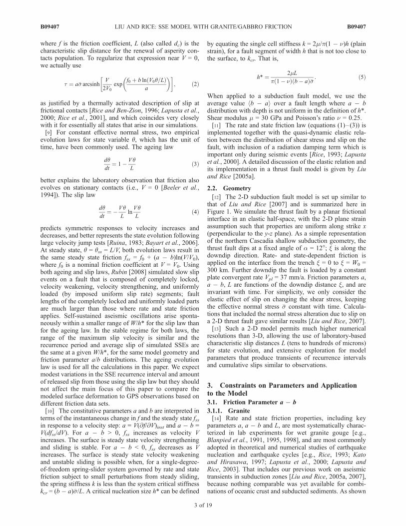
[33] Figures 8a and 8b illustrate the slip velocity historyduring modeled transient events, using wet granite andgabbro friction data set, respectively. Downdip distributionsof parameters are shown in Figure 3 for each model. Forreference, the plate convergence rate is Vpl = 37 mm/a�1.2 10�9 m/s. Only the depth range involved in thetransient slip is plotted. For the wet granite profile, thefriction stability transition is at downdip 66 km, and the low�s zone from 46 to 86 km. For the gabbro profile, thestability transition is at downdip 180 km, and the low �szone from 130 to 215 km. In both models, two nucleationfronts slowly march toward each other within the velocity-weakening zone low �s zone, before they merge and reachthe maximum slip velocity. Slip then propagates in bothupdip and downdip directions along the fault. The updippropagation continues at a relatively constant speed until itencounters the abrupt increase to high �s = 50 MPa. Down-dip propagation speed in the wet granite model is compa-rable to the updip speed before it reaches the stabilitytransition, further downdip from which the propagationspeed is rapidly reduced due to the increase of a � b tovelocity strengthening over a short distance. Following themaximum velocities in respective slip marching fronts, weestimate the slip propagation speed vr to be about 9 km/d inthe velocity-weakening zone. The entire process when sliprate is higher than 102Vpl is less than 0.01 year, or about3 days. The downdip propagation in the gabbro modelgradually slows down as a � b increases toward velocity

strengthening over a relatively long distance. Nevertheless,vr for the first 20 km propagation is about 3 km/d in bothupdip and downdip directions. Similar along-strike slippropagation speeds are expected in a 3-D simulation withthe same parameters and model resolution. Slip velocitycontinues to be higher than Vpl for about 0.1 year, but themoment is mostly released in less than 0.05 year, or about15 days. In addition to the differences in slip propagationspeed and event duration, we also note that for the gabbromodel after a maximum slip velocity of 1.6 10�4 m/sis reached at the center of transient nucleation zone at t�0.07 year, slip velocity quickly falls to between 10�7 and10�6 m/s along the propagating fronts. For the wet granitemodel, a maximum slip velocity of 1.8 10�6 m/s is alsoreached at the center of nucleation zone. However, thepropagating fronts continue to slip at high velocitiesbetween 10�7 and 10�6 m/s, before they encounter thebarriers of high effective normal stress or friction stabilitytransition.

4.3. Comparison to GPS

[34] An example of transient and intertransient slip down-dip distributions in a 5-year time window, using the wetgranite friction data, is shown in Figure 9a. Four episodesof transients are included, each releasing a maximum slipof about 23 mm in the velocity-weakening low �s zone.Much smaller slip takes place in the downdip velocity-strengthening region. Intertransient slip rate is calculated asan average rate during the period between sampled tran-sients when Vmax on the fault is Vpl. Transient slip isrecorded as the cumulative slip on the fault when Vmax

exceeds 2Vpl. This would include the transient nucleationphase and posttransient relaxation, and, for the wet graniteprofile, corresponds to the slip (gaps in Figure 9a) releasedin about 0.1 year, a duration twice of that shown in Figure 8.However, more than 90% of slip is released during the high-velocity period in Figure 8.

Figure 8. Slip velocity history during one transient event, using (a) wet granite (parameters inFigure 3a), and (b) gabbro (parameters in Figure 3b) friction data sets. The term log10(V) in m/s iscontoured. For reference, Vpl = 37 mm/a � 1.2 10�9 m/s. Vertical dashed line plots the position offriction stability transitions. For wet granite profile, low �s zone is from 46 to 86 km. For gabbro profile,low �s zone from is 130 to 215 km. Arrows show the along-dip bilateral slip propagation directions. Theparameter vr is the estimated propagation speed.

B09407 LIU AND RICE: SSE MODEL WITH GRANITE/GABBRO FRICTION

11 of 19

B09407

[35] To calculate surface deformation, we extrapolate the2-D transient slip and intertransient slip rate, which arevariables of the downdip distance, to 3-D distributions,assuming both follow an along-strike profile function b =4(1/2 � x/Lstrike)(1/2 + x/Lstrike). Here Lstrike = 500 km isthe approximate along-strike fault length that is affectedduring slow slip events in northern Cascadia, and x variesbetween �Lstrike/2 and Lstrike/2. The parameter b is atmaximum of 1.0 at the center x = 0 and decreases alongstrike to 0 at each edge (Figure 9b). The extrapolated 3-Dtransient slip distribution, using the wet granite friction data,is shown in Figure 9c.[36] The northern Cascadia trench is simplified by a

straight line oriented 34.16� NNW, as an approximation tothe Juan de Fuca and North American plate boundary(Figure 10). The fault along-strike center is aligned withGPS station PGC5 in the direction perpendicular to thesimplified trench line. Okada’s [1992] solution for disloca-tions in an elastic half-space is used to calculate the surfacedeformation and deformation rate due to the extrapolatedtransient slip and intertransient slip rate on the fault.[37] Here, GPS measurements of intertransient deforma-

tion rate are analyzed by McCaffrey [2009] for permanentstations ALBH, NANO, NEAH, SEAT, SEDR and UCLU,where nine episodes of slow slip events have been reportedfrom continuous observations for more than one decade. Forstation PGC5 that is not included in the McCaffrey [2009]analysis, we approximate the intertransient deformationrates as their 6.6-year average secular velocities [Mazzottiet al., 2003] multiplied by a factor of 1.6, which is estimatedbased on other stations where both types of deformationrates are available. For example, the ratio between theintertransient and secular velocities at station ALBH is alsoabout 1.6 [Dragert et al., 2004]. GPS measurements oftransient deformation are from observations of the 1999slow slip event in northern Cascadia [Dragert et al., 2001],

with intertransient motion removed assuming an eventduration of 15 days at each station.4.3.1. Wet Granite[38] Using wet granite friction data, the extrapolated 3-D

distribution of intertransient slip rate, with Vpl removed, isprojected on the surface in Figure 10a. Detailed modelparameters are in Figure 3a. The firmly locked faultsegment near the surface (dark color) is consistent withthe complete interseismic locking at the shallow �60 kminferred from leveling lines and tide gauge data in northernCascadia [Hyndman and Wang, 1995]. However, the wetgranite friction model predicts an abrupt change fromcomplete locking to nearly free slipping at downdip�60 km (sudden change from dark to light color), whilethe Hyndman and Wang [1995] model requires slip rate onthe following �60 km of fault segment to linearly increasefrom 0 to Vpl, in order to better explain the long-termgeodetic data. As a result, the predicted intertransientsurface deformation rate (horizontal component shownhere) only agrees reasonably well with GPS observationsat two coastal stations but cannot explain signals at most ofthe inland stations. Cumulative aseismic slip is projected onthe surface as shown in Figure 10b. Slip of more than 20 mmconcentrate in a relatively narrow along-dip region,corresponding mostly to the assumed low �s zone updipfrom the friction stability transition. Modeled deformationagain can only explain observations at the coastal stations,but fails to match those at stations further away from thetrench.[39] To quantify the comparison between observed and

modeled deformation and deformation rate, we define amisfit function

c2 ¼ 1

N

XNi¼1

~xcali �~xobsi

� �2~s2i

; ð8Þ

Figure 9. (a) Cumulative slip in a 5-year window, including four episodes of SSEs, using wet granitefriction. Slip lines are plotted every 0.1 year. Vertical dashed line denotes the friction stabilitytransition. During each SSE, maximum slip of about 23 mm is released in the velocity-weakening low�s zone, with much smaller slip in the downdip velocity-strengthening zone. Peak at �30 kmcorresponds to the nucleation front for the next megathrust earthquake. (b) Along-strike distributionfunction b(x) = 4(1/2 � x/Lstrike)(1/2 + x/Lstrike); x is along-strike distance, from �250 to 250 km, andLstrike = 500 km. (c) Extrapolated 3-D transient slip (mm), based on the 2-D distribution in Figure 9a andmultiplied by b(x).

B09407 LIU AND RICE: SSE MODEL WITH GRANITE/GABBRO FRICTION

12 of 19

B09407

where ~xical and ~xi

obs are model predicted and observedhorizontal displacement vectors, and ~si is the standardderivation at the ith station. Total station number N = 7. Forthe case shown in Figure 10, transient deformation misfit isctran2 = 127.6 and intertransient deformation rate misfit is

cinter2 = 76.6. Similar cumulative aseismic slip and

recurrence period are produced using W = 30 km, �s =0.45 MPa and L = 0.4 mm (W/h* = 5; see Figure 6). Whenthe model results are compared to GPS measurements, themisfit functions are ctran

2 = 125.7 and cinter2 = 73.0. We

expect simulations from other groups of W using the wet

granite data will have even larger misfits as the slip arearemains shallow but narrower.4.3.2. Gabbro[40] A group of simulation cases that produce transients

of slip 20–30 mm and recurrence period of �2 years arelisted in Table 2, corresponding to cases in the dashed lineboxes in Figure 7. W/h* ranges from 12.4 to 17.3, due todifferent sets of W and �s; L is uniformly 0.16 mm in allcases. The parameter dmax is the maximum cumulativeaseismic slip on the fault. The parameter dmax is usuallylocated at the center of the slip nucleation zone, wherevelocity reaches maximum as shown in Figure 8. Amongthe listed cases, misfit function ctran

2 is smallest for case e:W = 50 km, �s = 1.2 MPa and L = 0.16 mm. However, thelimited number of simulation cases does not guarantee thisis the best fitting model using the gabbro friction data. Foreach set of W and W/h* (�s/L is thus determined), the linearscaling of d with L allows us to calculate ctran

2 for a suite oftransient slip downdip distributions d(x) without actuallyperforming the earthquake and slow slip sequences simu-lations. For example, we expect that, with W = 35 km,W/h* = 12.4 and �s = 4 MPa (thus L = 0.32 mm), d(x) is justtwice of the slip on the fault from model a, with dmax =36.8 mm. The recurrence period also becomes twice longerof that from model a. The term ctran

2 = 35.0 for the newdistribution d(x). Each curve in Figure 11 is calculatedbased on such scaling relation for the same W and W/h*.For models with the same W but different W/h* (e.g., a andb, c and d), the ctran

2 versus dmax curves are very close toeach other with similar minimum. For W = 35 km (blacklines), the minimum ctran

2 is reached at dmax � 40 mm. Thisimplies a recurrence period between 3.2 and 4.3 years,which is much longer than the observed interval in Casca-dia, suggesting that W = 35 km is not a good estimate of thefault length of the velocity-weakening low �s zone in orderto fit the transient surface deformation. It is clear thatmodels with W = 40 km cannot best fit the observationseither. Both models e and f have ctran

2 near the minimumvalues, with dmax about 25 mm and recurrence period about1.75 years and can be considered as best fitting models forthe transient slip.[41] The extrapolated 3-D distribution of intertransient

slip rate and transient slip based on model e are projected onthe surface in Figures 12a and 12b, respectively. Detailedmodel parameters are in Figure 3b. The downdip end of

Figure 10. Comparison between observed (red arrows)and model predicted (blue arrows) intertransient deforma-tion rate and transient deformation, using the wet granitefriction data. Model parameters are shown in Figure 3a.(a) Intertransient slip rate, with Vpl = 37 mm/a removed,projected on the surface. Along-strike center aligned withstation PGC5 is perpendicular to the simplified straighttrench line (dashed). Dark colors represent strong inter-seismic locking, and light colors represent transition to freesliding at Vpl. Error ellipses are double the 95% confidencelimits derived from regression errors [Mazzotti et al., 2003;McCaffrey, 2009]. (b) Transient slip, with intertransient slipremoved, projected on the surface. Error ellipses are doublethe 95% confidence limits reported by Dragert et al. [2001].Error contribution from the intertransient slip rate isnegligible compared that from transient slip because ofthe assumed short event duration of 15 days at each station. Table 2. Model Cases Using the Gabbro Friction Dataa

ModelW

(km)�s

(MPa)L

(mm) W/h*dmax

(mm) ctran2 cinter

2

a 35 2.0 0.16 12.4 18.4 79.2 141.8b 35 2.8 0.16 17.3 24.7 55.5 151.4c 40 1.6 0.16 12.9 20.0 53.5 147.9d 40 2.0 0.16 16.2 24.6 37.4 145.7e 50 1.2 0.16 15.2 24.1 22.7 142.2f 55 1.0 0.16 15.3 25.8 23.5 143.5aWith different parameter sets of W, �s, and L that produce episodic

aseismic slip between 18 and 25 mm and recurrence period between 1 and2 years. The parameter dmax is the maximum accumulated slip on the fault,located at the center of the slip nucleation zone, where maximum velocity isreached (Figure 8). Misfit ctran

2 is smallest for model e: W = 50 km, �s =1.2 MPa, and L = 0.16 mm. Intertransient slip rate misfit is uniformly largefor all model cases.

B09407 LIU AND RICE: SSE MODEL WITH GRANITE/GABBRO FRICTION

13 of 19

B09407

complete interseismic locking extends to �100 km from thetrench, followed by a gradual transition to stable slidingnear Vpl at �200 km downdip distance. The locked andtransitional slip fault lengths are larger than those inferredfrom long-term geodetic data [Hyndman and Wang, 1995]and are primarily responsible for the overprediction of theshort-term intertransient deformation rate as shown inFigure 12a. The depth of complete interseismic locking ismainly determined by the distribution of a � b in theseismogenic zone, which, for gabbro because of the largescatter in measurements at 250�C, we assume to be aconstant of �0.0035 up to T = 416�C (corresponding todowndip �95 km) at supercritical water conditions. Futurelaboratory experiments on gabbro friction properties atintermediate temperatures should help to better constrainthe depth of interseismic locking. Aseismic slip of morethan 20 mm are distributed within the �80 km along-diplow �s zone, which is much further inland than the modelusing wet granite data. The comparison to GPS measure-ments of transient deformation is significantly improved atmost stations.[42] The simple planar fault model presented in this paper

does not take into consideration any geometry variationsalong the trench or with depth, while 3-D subduction slabmodels [Fluck et al., 1997] do suggest slab curvaturesbeneath the southern Vancouver Island. Depth contours ofthe plate interface approximately follows the orientation ofthe trench (thick black line). This partly explains the largediscrepancies in transient deformation comparison at sta-tions that are far from the center of the slip area, e.g., UCLUand SEAT. Incorporation of a more realistic fault geometryshould reduce the discrepancies at those stations. Forinstance, if the slip area shown in Figure 12b follows the

curved trench line, model predicted displacement wouldimprove at station UCLU and reduce at SEAT. Anotheruncertainty is that in using Okada’s [1992] solution tocalculate surface deformation we do not consider the spatialvariations in the elastic properties of the lithosphere. Instead,constant shear modulus of 30 GPa and Poisson’s ratio of0.25 have been used, while seismic reflection imaging innorthern Cascadia reveals complex regional structuresbeneath the Vancouver Island [Calvert, 2004].

5. Discussion

5.1. Wet Granite and Gabbro Friction Dataand Implication for Downdip Limit of Seismogenesis

[43] Previous studies on modeling episodic slow slipevents [Shibazaki and Iio, 2003; Liu and Rice, 2005a,2007; Shibazaki and Shimamoto, 2007; Rubin, 2008]showed that aseismic transients emerge as a natural outcomeof the laboratory-revealed rate and state friction processes atcertain depth-variable friction parameter and effective nor-mal stress distributions. Numerical models can producefeatures, such as the average velocity, cumulative aseismicslip and recurrence interval, qualitatively similar to those

Figure 12. Comparison between observed (red arrows)and model predicted (blue arrows) intertransient deformationrate and transient deformation, using the gabbro friction data.Model parameters are shown in Figure 3b. (a) Intertransientslip rate and (b) transient slip. See Figure 10 caption fordetails.

Figure 11. Dependence of ctran2 on modeled aseismic slip

dmax. Each curve is calculated based on the scaling betweenslip downdip distribution d(x) and L and the linear relationbetween surface deformation and d(x), for fixedW andW/h*.Black indicates W = 35 km, W/h* = 12.4 (solid) and 17.3(dashed). Red indicates W = 40 km, W/h* = 12.9 (solid) and16.2 (dashed). Blue indicates W = 50 km, W/h* = 15.2.Green indicates W = 55 km, W/h* = 15.3. Models a–f listedin Table 2 are also plotted as individual dots on the curves.

B09407 LIU AND RICE: SSE MODEL WITH GRANITE/GABBRO FRICTION

14 of 19

B09407

inferred for natural events. However, no comparison be-tween model predicted and geodetically observed (by GPSat most subduction zones) transient deformation has yetbeen made. A large uncertainty in attempts to compare thesetwo is our limited knowledge of appropriate friction prop-erties to use in the subduction fault models. Friction data, inparticular, the temperature-dependent stability parameter a� b, applied in some of the above studies that considerdepth-variable properties, are from wet granite gouge,which has been well studied under hydrothermal conditionsbut is not a good representation of the oceanic crust.Speculations about reexamination of the rate and statefriction data have been proposed by Liu and Rice [2007].In this paper, we apply both wet granite [Blanpied et al.,1998] and recently reported gabbro gouge friction data [Heet al., 2007] to a Cascadia-like 2-D subduction fault, tomodel aseismic transients and compare the resulting surfacedeformation to GPS observations along the northern Casca-dia margin. The major differences between the gabbro andwet granite friction data are (1) velocity weakening tostrengthening stability transition occurs at a higher temper-ature around 510�C for gabbro gouge under supercriticalwater conditions, compared to �350�C for wet granite and(2) the absolute values of high-temperature velocitystrengthening a � b is approximately 1 order of magnitudesmaller for gabbro than for wet granite. When the frictionparameters are converted to be depth-variable using athermal model of the northern Cascadia subduction zone,these differences result in a much deeper friction stabilitytransition, a wider and less stabilizing transition zone forgabbro.[44] One natural and practical question that arises from

the two dramatically different depth distributions of a � bfrom wet granite and gabbro friction experiments, as shownin Figure 3 (top), is what are their implications for thedowndip end of a megathrust earthquake rupture. Using thecurrent model and parameters in Figure 3, for the gabbrofriction profile, subduction earthquake rupture propagatesbeyond the stability transition at �180 km to downdip�250 km. The extended propagation in the velocity-strengthening zone is facilitated by the small a � b > 0on the deeper part of the fault. For the wet granite frictionprofile, earthquake rupture also propagates a bit furtherdowndip from the stability transition (downdip 66 km) to�85 km, as a result of the highly stabilizing effect of largea � b > 0. While no large subduction earthquake hasoccurred along the Cascadia margin in the past 300 yearsfor a direct measurement, long-term geodetic observationsusing repeated leveling lines, gravity profiles (time span 4 to44 years) and tide gauge data (time span 22 to 80 years) arebest fit by a completely locked 60 km along-dip segmentfollowed by another 60 km segment with linear increase ofslip rate from 0 to Vpl [Dragert et al., 1994; Hyndman andWang, 1995]. This would suggest a downdip limit ofseismic rupture somewhere between 60 and 120 km. Thus,the gabbro friction data can predict transient slip in reason-able agreement with GPS observations, but also overpredictthe downdip extent of seismic rupture indicated by long-term geodetic measurements.[45] Incorporation of fault gouge dilatancy to the friction-

al strength evolution appears to be a promising mechanismto reconcile this discrepancy. Segall and Rice [1995]

showed that fault stabilization by induced suction fromdilatancy during accelerated slip becomes most importantat extremely high fluid pressure (i.e., low �s), a situationproposed for the occurrence of short-period transients.Including dilatancy in a 2-D subduction fault model withrate and state friction, Taylor and Rice [1998] found thatquasi-dynamic seismic rupture slows down or even stopsnear the surface where effective normal stress is lower thanthat in the seismogenic zone; seismic slip of several meterswould occur at the trench without dilatancy. Building on thework by Taylor and Rice [1998], Liu and Rice [2005b] andespecially Segall and Rubin [2007], we analyze the con-ditions for short-period aseismic transients and dimensionsof coseismic rupture of a fluid infiltrated subduction faultincluding dilatancy and pore compaction effects, with amembrane diffusion approximation [Liu et al., 2008]. Notonly episodic aseismic transients now exist for a muchbroader range of W/h* due to dilatancy stabilization at low�s, the quasi-dynamic seismic rupture speed and spatialextent can also be significantly reduced. Assuming anintermediate fault drainage, i.e., the characteristic diffusiontime for fault gouge fluid pressure to reequilibrate with itsambient level is comparable to the characteristic stateevolution time, seismic rupture stops updip of the frictionstability transition and causes nearly no coseismic slip at thetrench, using dilatancy parameters consistent with labexperiments [Marone et al., 1990; David et al., 1994]. Thissuggests that a subduction fault extending well downdip ofthe seismogenesis could be frictionally unstable (a � b < 0)but undergo no seismic slip due to the existence of highfluid pressure and effective dilatancy stabilization, andprovides a possible explanation to the inferred ‘‘gap’’between depths of seismic rupture and slow slip events innorthern Cascadia.

5.2. ‘‘Ageing’’ and ‘‘Slip’’ Evolution Laws

[46] As a physical mechanism for episodic slow slipevents, fault models using the slip law have generallysimilar results to those using the ageing law (this paper).Both laws predict fault responses evolving from oscillatorydecay, to aseismic simple periodic, complex periodic, andeventually seismic instability as the key parameter W/h*increases. Spontaneous aseismic oscillations arise at similarW/h* but are limited within a much smaller range using theslip law than ageing law. For example, for simulation caseswith the same subduction fault geometry and frictionparameters, Rubin [2008] found that transients only appearwhen W/h* is between 2 and 4.5 for slip law, and between 2and 13 for ageing law. This difference may become insig-nificant with the incorporation of dilatancy, which caneffectively delay the onset of seismic instability thus pro-duce aseismic transients at much larger W/h* [Liu et al.,2008]. Although there are subtle differences in the aseismic‘‘rupture’’ processes modeled with the two evolution laws,aseismic slip in both cases is mostly attributed to the low �szone updip from the friction stability transition [Rubin,2008]. In addition, modeling results including normalizedmaximum moment rate, maximum slip velocity, recurrenceinterval and cumulative slip during each cycle with theageing law are in similar ranges to their respective counter-parts with the slip law. For both the wet granite and gabbrofriction data profiles, parameter space exploration as de-

B09407 LIU AND RICE: SSE MODEL WITH GRANITE/GABBRO FRICTION

15 of 19

B09407

scribed in section 4 can also be performed using the sliplaw, to identify appropriate parameter sets that produceaseismic transients of slip and period close to observations.Similarly, we expect model results using the gabbro datacan better explain the transient surface deformation innorthern Cascadia.

5.3. Two- and Three-Dimensional Simulations

[47] In this study, frictional strength and sliding velocityevolution are calculated as functions of the downdip dis-tance and of time, thus providing a 2-D model. In theevolution process, all properties are assumed to be uniformalong the strike direction (plane strain). Cumulative tran-sient slip as a function of depth is extrapolated to slip on afault plane that spans Lstrike = 500 km along the strikedirection, by assuming an along-strike distribution function.Such a 2-D model setup allows us to explore the parameterspace extensively to know how properties such as slip,recurrence interval and maximum velocity change as keyparameters W, �s and L vary in the constrained ranges, forboth friction data sets used in this study. Comparisonsbetween GPS observations and numerically predicted sur-face displacements based on a large group of models arealso possible in order to determine the best fitting parametersets.[48] Modeling of slow slip events on a 3-D subduction

fault governed by rate and state friction has been reported ina previous work [Liu and Rice, 2005a] before our recogni-tion of near-lithostatic fluid pressure in SSE source areas; auniformly high effective normal stress �s = 100 MPa wasused in the entire seismogenic zone and further downdip.Aseismic transients emerge spontaneously around the fric-tion stability transition, and migrate along the strike atspeeds much slower than the observed 5–15 km/d inCascadia. Faster migration was found when �s reduces to50 MPa [Liu and Rice, 2005b]. Although multiple transientscan emerge during the interseismic period, regularly recur-ring events were not identified in those 3-D simulationswith high �s. The near-lithostatic fluid pressure propositionwas adopted in a recent 3-D slow slip modeling study byShibazaki and Shimamoto [2007], who used a small cutoffvelocity of 10�7 to 10�6 m/s to control the aseismic slip rateacceleration and deceleration. Under conditions of �s �1 MPa and L � 0.8 mm on the deeper plate interface,short-period SSEs with along-strike migration speeds andslip velocities of 4–8 km/d and 2–4 10�7 m/s, respec-tively, can be produced. The slow slip along-strike migra-tion speed vr is found to be proportional to the maximumslip velocity following the relation first obtained by Ida[1973] for a mode II elastodynamic rupture

vr

Vmax

¼ gm0

Dtp�r; ð9Þ

where g is of order of unity and Dtp�r is the peak toresidual shear stress drop. Equation (9) was also confirmedin the context of slow slip events for along-dip ‘‘rupture’’propagation on a 2-D fault with updip completely locked[Rubin, 2008]. The modeled slow slip ‘‘rupture’’ in thisstudy, as shown in Figure 8, propagates in both updip anddowndip directions, with vr � 3–9 km/d and Vmax � 10�6

to 10�7 m/s. As the proportionality between vr and Vmax

holds for along-strike propagation, we expect (but cannotverify due to current computational limitations) that in a 3-Dmodel with parameters as presented in this paper lateralmigration of slow slip along the trench, like observed innorthern Cascadia, would also be produced. The cumulativetransient slip distribution from such 3-D models would bemore realistic than that extrapolated based on the 2-Dmodels. However, the slow slip would be expected toremain in the same depth range as shown in Figures 10band 12b, which are determined by the depth-variable modelparameters for each friction data set. Thus, the comparisonsbetween observed and modeled surface deformation shouldbe qualitatively similar to what we present here.

6. Conclusion

[49] We apply the ageing version of the rate and statefriction law with a single state variable and depth-dependentfriction properties to a two-dimensional thrust fault model tosimulate episodic slow slip events in shallow subductionzones. Laboratory friction data on wet granite and gabbrogouges are applied to a 2-D fault with a Cascadia-likegeometry and thermal profile. Gabbro is an essential partof the oceanic crust and chemically equivalent to basalt,thus a much better proxy than wet granite for the subductioninterface studied in this paper. In contrast to the wet granite�350�C unstable to stable transition, sliding on the gabbrogouge continues to be velocity weakening up to T � 510�Cunder supercritical water conditions. The high-temperaturevelocity-strengthening regime is much less stabilizing thanthat of wet granite at similar temperatures, due to the nearly1 order of magnitude smaller a � b > 0 up to 600�C. Whenthe friction data are converted to be depth-variable param-eters using a thermal model of the northern Cascadiasubduction zone, these differences result in a much deeperfriction stability transition, with a wider and less stabilizingtransition zone for gabbro.[50] Existence of high fluid pressure in the source areas of

slow slip events and nonvolcanic tremors have beensuggested by seismological observations, petrological andthermal structures in shallow dipping subduction zones.Near-lithostatic fluid pressure is essential to the occurrenceof sustained short-period aseismic oscillations in subductionfault models based on rate and state friction. In this paper,we constrain the depth range of generally overhydrostaticand near-lithostatic fluid pressure zones by incorporatingthe oceanic crust metamorphic phase diagram and thermalstructures of the southwest Japan and northern Cascadiasubduction zones. We first identify plausible spatial corre-spondence between seismically inferred high fluid pressurezone and the depths of major dehydration reactions due tomineral phase changes in the SW Japan subduction zone.Dense instrumentation there such as Hi-net borehole sta-tions has facilitated the precise relocation of nonvolcanictremors, including low-frequency earthquakes, an indicatorof high fluid pressure. An analogy of the spatial correspon-dence is drawn to the northern Cascadia subduction zone,where dehydration reaction depths are also determined byits petrological and thermal structures, to estimate thedistribution of fluid pressure along the interface. Fluidpressure is generally high (overhydrostatic) at depths wheremajor water-releasing phase transitions take place, as well

B09407 LIU AND RICE: SSE MODEL WITH GRANITE/GABBRO FRICTION

16 of 19

B09407

as the surrounding areas due to fluids permeation. Inparticular, near-lithostatic fluid pressure is possible aroundthose phase transitions with the most water weight percentreductions, e.g., epidote blueschist to eclogite on the top ofthe slab and epidote amphibolite to eclogite on the bottomof the slab. The estimated fluid pressure distribution isconsistent with inferred high vp/vs and Poisson’s ratios fromat least 20 to 45 km in depth along the northern Cascadiasubduction zone from a recent study using convertedseismic waveforms [Audet et al., 2009]. The fluid pressuredistribution conjecture is further simplified in our model tohave an extremely low effective normal stress zone aroundthe friction stability transition, embedded in uniformly high�s on the rest of the fault (except near the surface).[51] For a suite of forward models examined, spontane-

ous aseismic transients emerge within a limited range ofW/h*, which is determined by independently chosen valuesof W, low �s and L in consistency with laboratory andobservational constraints. W/h* is �2 to 7 for wet graniteand �6 to 16 for gabbro. For both friction profiles, thecumulative aseismic slip, recurrence interval and maximumslip velocity increase withW/h*. Without following a formalinversion procedure and performing true 3-D calculations,we search for parameter sets W, �s and L that producedaseismic transient of slip 20–30 mm and recurrence interval1–2 years. L is chosen to be as close to the lab values(�10s mm) as possible, and extremely small effectivenormal stress �s of a few MPa in the transition zone is used.For such simulation cases, we found that aseismic slipnucleates in the velocity-weakening low �s zone and slippropagates bilaterally at roughly the same speed of 3–9 km/din both directions before encountering the updip high �sbarrier and downdip stability transition, respectively. Along-strike migration at similar speeds is expected in 3-Dcalculations with the same parameters. Most of the aseismicslip takes place within the low �s velocity-weakening zone.Modeled 2-D transient slip and intertransient slip rate areextrapolated to 3-D, assuming an along-strike distributionfunction, to calculate the surface deformation and deforma-tion rate using Okada’s [1992] solution for dislocation in anelastic half-space with constant shear modulus and Poisson’sratio. Transient slip modeled with the wet granite frictiondata is concentrated in a narrow strip mostly offshore.Except for two coastal stations, only small fractions of theGPS measurements of both transient deformation and inter-transient deformation rate at the inland stations can bereproduced. Modeled transient deformation using the gabbrodata can fit the GPS measurements fairly well with a faultlength of 50 to 55 km updip from the stability transition underlow effective normal stress of �1 MPa and L = 0.16 mm.However, the intertransient deformation rate is generallyoverpredicted due to the deep interseismic locking at�100 km downdip. Future experiments on gabbro gougesto measure friction parameters at seismogenic conditionsshould provide more constraints on the fault locking depth.[52] Although a more realistic model for such compar-

isons would incorporate effects such as spatial variations inthe geometry and mechanical properties of the subductionslab and the overlying lithosphere, we show that applicationof reasonably appropriate rate and state friction data has thefirst order of importance for the forward models to produceresults that can be constrained by field observations. For the

northern Cascadia subduction margin, friction properties ofgabbro gouge seem to do a much better job than the widelyused wet granite data. Further laboratory experiments ongabbro and other oceanic crust rocks at elevated temper-atures will shed more lights on the mechanism of aseismicdeformation transients and possibly nonvolcanic tremors insubduction zones.

[53] Acknowledgments. We thank Hiro Noda, who first pointed us toHe et al.’s [2006] experimental work on gabbro; Changrong He, whoprovided his then unpublished data and continued discussion on frictionalexperiments on gabbro gouge; Robert McCaffrey for providing his GPSdata analysis; and two anonymous reviewers for their comments that helpedto improve the manuscript. We also thank Nora DeDontney for her code toextrapolate a 2-D slip distribution to three dimensions, and we thank AllanM. Rubin and Paul Segall for discussions on effects of dilatancy. This studywas initiated at Harvard under support of NSF-EAR award 0510196 andUSGS-NEHRP award 07HQGR0057 and continued at Princeton under aDepartment of Geosciences Hess postdoctoral fellowship to Yajing Liu andUSGS-NEHRP award 08HQGR0047 to Allan Rubin that partly supportedY. Liu.

ReferencesAudet, P., M. G. Bostock, N. I. Christensen, and S. M. Peacock (2009),Seismic evidence for overpressured subducted oceanic crust and mega-thrust fault sealing, Nature, 457, 76–78, doi:10.1038/nature07650.

Bayart, E., A. M. Rubin, and C. Marone (2006), Evolution of fault frictionfollowing large velocity jumps, Eos Trans. AGU, 87(52), Fall Meet.Suppl., Abstract S31A-0180.

Beeler, N. M., T. E. Tullis, and J. D. Weeks (1994), The roles of time anddisplacement in the evolution effect in rock friction, Geophys. Res. Lett.,21, 1987–1990, doi:10.1029/94GL01599.

Blanpied, M. L., D. A. Lockner, and J. D. Byerlee (1991), Fault stabilityinferred from granite sliding experiments at hydrothermal conditions,Geophys. Res. Lett., 18, 609–612, doi:10.1029/91GL00469.

Blanpied, M. L., D. A. Lockner, and J. D. Byerlee (1995), Frictional slip ofgranite at hydrothermal conditions, J. Geophys. Res., 100(B7), 13,045–13,064, doi:10.1029/95JB00862.

Blanpied, M. L., C. J. Marone, D. A. Lockner, J. D. Byerlee, and D. P. King(1998), Quantitative measure of the variation in fault rheology due tofluid-rock interactions, J. Geophys. Res., 103(B5), 9691 – 9712,doi:10.1029/98JB00162.

Brooks, B. A., J. H. Foster, M. Bevis, L. N. Frazer, C. J. Wolfe, andM. Behn (2006), Periodic slow earthquakes on the flank of Kilaueavolcano, Hawai’i, Earth Planet. Sci. Lett., 246(3 – 4), 207 – 216,doi:10.1016/j.epsl.2006.03.035.

Calvert, A. J. (2004), Seismic reflection imaging of two megathrust shearzones in the northern Cascadia subduction zone, Nature, 428(6979),163–167, doi:10.1038/nature02372.

Chester, F. M., and N. G. Higgs (1992), Multimechanism friction consti-tutive model for ultrafine quartz gouge at hypocentral conditions,J. Geophys. Res., 97(B2), 1859–1870, doi:10.1029/91JB02349.

Chlieh, M., J. P. Avouac, K. Sieh, D. H. Natawidjaja, and J. Galetzka(2008), Heterogeneous coupling of the Sumatran megathrust constrainedby geodetic and paleogeodetic measurements, J. Geophys. Res., 113,B05305, doi:10.1029/2007JB004981.

Currie, C. A., R. D. Hyndman, K. Wang, and V. Kostoglodov (2002),Thermal models of the Mexico subduction zone: Implications for themegathrust seismogenic zone, J. Geophys. Res., 107(B12), 2370,doi:10.1029/2001JB000886.

David, C., T.-F. Wong, W. Zhu, and J. Zhang (1994), Laboratory mea-surements of compaction-induced permeability change in porous rocks:Implications for the generation and maintenance of pore pressure excessin the crust, Pure. Appl. Geophys., 143, 425–456, doi:10.1007/BF00874337.

Dieterich, J. H. (1979), Modeling of rock friction 1. Experimental resultsand constitutive equations, J. Geophys. Res., 84(B5), 2161– 2168,doi:10.1029/JB084iB05p02161.

Dragert, H., R. D. Hyndman, G. C. Rogers, and K. Wang (1994), Currentdeformation and the width of the seismogenic zone of the northernCascadia subduction thrust, J. Geophys. Res., 99(B1), 653 – 668,doi:10.1029/93JB02516.

Dragert, H., K. Wang, and T. S. James (2001), A silent slip event on thedeeper Cascadia subduction interface, Science, 292, 1525 – 1528,doi:10.1126/science.1060152.

Dragert, H., K. Wang, and G. Rogers (2004), Geodetic and seismic signa-tures of episodic tremor and slip in the northern Cascadia subductionzone, Earth Planets Space, 56(12), 1143–1150.

B09407 LIU AND RICE: SSE MODEL WITH GRANITE/GABBRO FRICTION

17 of 19

B09407

Fluck, P., R. D. Hyndman, and K. Wang (1997), Three-dimensional dis-location model for great earthquakes of the Cascadia subduction zone,J. Geophys. Res., 102(B9), 20,539–20,550, doi:10.1029/97JB01642.

Gomberg, J., J. L. Rubinstein, Z. Peng, K. C. Creager, J. Vidale, andP. Bodin (2008), Widespread triggering of nonvolcanic tremor in Cali-fornia, Science, 319, 173 , doi:10.1126/science.1149164.

Hacker, B. R., G. A. Abers, and S. M. Peacock (2003), Subduction factory1. Theoretical mineralogy, densities, seismic wave speeds, and H2O con-tents, J. Geophys. Res., 108(B1), 2029, doi:10.1029/2001JB001127.

He, C., W. Yao, Z. Wang, and Y. Zhou (2006), Strength and stability offrictional sliding of gabbro gouge at elevated temperatures, Tectonophy-sics, 427, 217–229, doi:10.1016/j.tecto.2006.05.023.

He, C., Z. Wang, and W. Yao (2007), Frictional sliding of gabbro gougeunder hydrothermal conditions, Tectonophysics, 445, 353 – 362,doi:10.1016/j.tecto.2007.09.008.

Hirose, H., K. Hirahara, F. Kimata, N. Fujii, and S. Miyazaki (1999), Aslow thrust slip event following the two 1996 Hyuganada earthquakesbeneath the Bungo Channel, southwest Japan, Geophys. Res. Lett., 26,3237–3240, doi:10.1029/1999GL010999.

Hyndman, R. D., and K. Wang (1995), The rupture zone of Cascadia greatearthquakes from current deformation and the thermal regime, J. Geo-phys. Res., 100(B11), 22,133–22,154, doi:10.1029/95JB01970.

Ida, Y. (1973), The maximum acceleration of seismic ground motion, Bull.Seismol. Soc. Am., 63, 959–968.

Ide, S., D. R. Shelly, and G. C. Beroza (2007), Mechanism of deep lowfrequency earthquakes: Further evidence that deep non-volcanic tremor isgenerated by shear slip on the plate interface, Geophys. Res. Lett., 34,L03308, doi:10.1029/2006GL028890.

Kao, H., S. Shan, H. Dragert, G. Rogers, J. F. Cassidy, and K. Ramachandran(2005), A wide depth distribution of seismic tremors along the northernCascadia margin, Nature, 436, 841–844, doi:10.1038/nature03903.

Kao, H., S. Shan, H. Dragert, G. Rogers, J. F. Cassidy, K. Wang, T. S.James, and K. Ramachandran (2006), Spatial-temporal patterns of seis-mic tremors in northern Cascadia, J. Geophys. Res., 111, B03309,doi:10.1029/2005JB003727.

Kato, N. (2003), A possible model for large preseismic slip on a deeperextension of a seismic rupture plane, Earth Planet. Sci. Lett., 216(1–2),17–25, doi:10.1016/S0012-821X(03)00483-7.

Kato, N., and T. Hirasawa (1997), A numerical study on seismic couplingalong subduction zones using a laboratory-derived friction law, Phys. EarthPlanet. Inter., 102(1–2), 51–68, doi:10.1016/S0031-9201(96)03264-5.

Kodaira, S., T. Iidaka, A. Kato, J. O. Park, T. Iwasaki, and Y. Kaneda (2004),High pore fluid pressure may cause silent slip in the Nankai trough,Science, 304, 1295–1298, doi:10.1126/science.1096535.

Lachenbruch, A. H., and J. H. Sass (1973), Thermo-mechanical aspects ofthe San Andreas Fault system, in Proceedings of the Conference on theTectonic Problems of the San Andreas Fault System, edited by B. L.Kovach and A. Nur, Stanford University Publ. Geol. Sci., 13, 192–205.

Lapusta, N., and J. R. Rice (2003), Nucleation and early seismic propaga-tion of small and large events in a crustal earthquake model, J. Geophys.Res., 108(B4), 2205, doi:10.1029/2001JB000793.

Lapusta, N., J. R. Rice, Y. Ben-Zion, and G. Zheng (2000), Elastodynamicanalysis for slow tectonic loading with spontaneous rupture episodes onfaults with rate- and state-dependent friction, J. Geophys. Res., 105(B10),23,765–23,789, doi:10.1029/2000JB900250.

La Rocca, M., K. C. Creager, D. Galluzzo, S. Malone, J. E. Vidale, J. R.Sweet, and A. G. Wech (2009), Cascadia tremor located near plate inter-face constrained by S minus P wave times, Science, 323, 620–623,doi:10.1126/science.1167112.

Linde, A. T., M. T. Gladwin, M. J. S. Johnston, R. L. Gwyther, and R. G.Bilham (1996), A slow earthquake sequence on the San Andreas fault,Nature, 383(6595), 65–68, doi:10.1038/383065a0.

Liu, Y., and J. R. Rice (2005a), Aseismic slip transients emerge sponta-neously in three-dimensional rate and state modeling of subduction earth-quake sequences, J. Geophys. Res., 110, B08307, doi:10.1029/2004JB003424.

Liu, Y., and J. R. Rice (2005b), Pore pressure evolution in shallow subduc-tion earthquake sequences and effects on aseismic slip transients—Numerical modeling with rate and state friction, Eos Trans. AGU,86(52), Fall Meet. Suppl., Abstract T11E-05.

Liu, Y., and J. R. Rice (2007), Spontaneous and triggered aseismic defor-mation transients in a subduction fault model, J. Geophys. Res., 112,B09404, doi:10.1029/2007JB004930.

Liu, Y., A. M. Rubin, J. R. Rice, and P. Segall (2008), Role of faultdilatancy in subduction zone aseismic deformation transients and thrustearthquakes, Eos Trans. AGU, 89(53), Fall Meet. Suppl., AbstractS34B-04.

Lockner, D. A., and J. D. Byerlee (1986), Laboratory measurements ofvelocity-dependent frictional strength, U.S. Geol. Surv. Open File Rep.,86-417.

Lowry, A. R., K. M. Larson, V. Kostoglodov, and R. Bilham (2001), Tran-sient fault slip in Guerrero, southern Mexico, Geophys. Res. Lett., 28,3753–3756, doi:10.1029/2001GL013238.

Marone, C., C. B. Raleigh, and C. H. Scholz (1990), Frictional behaviorand constitutive modeling of simulated fault gouge, J. Geophys. Res.,95(B5), 7007–7025, doi:10.1029/JB095iB05p07007.

Mazzotti, S., H. Dragert, J. Henton, M. Schmidt, R. Hyndman, T. James,Y. Lu, and M. Craymer (2003), Current tectonics of northern Cascadiafrom a decade of GPS measurements, J. Geophys. Res., 108(B12),2554, doi:10.1029/2003JB002653.

McCaffrey, R. (2009), Time-dependent inversion of three-component con-tinuous GPS for steady and transient sources in northern Cascadia,Geophys. Res. Lett., 36, L07304, doi:10.1029/2008GL036784.

Miyazawa, M., and J. Mori (2006), Evidence suggesting fluid flow beneathJapan due to periodic seismic triggering from the 2004 Sumatra-Andaman earthquake, Geophys. Res. Lett., 33, L05303, doi:10.1029/2005GL025087.

Murray, J. R., and P. Segall (2005), Spatiotemporal evolution of a transientslip event on the San Andreas fault near Parkfield, California, J. Geophys.Res., 110, B09407, doi:10.1029/2005JB003651.

Obara, K. (2002), Nonvolcanic deep tremor associated with subduction insouthwest Japan, Science, 296, 1679 – 1681, doi:10.1126/science.1070378.

Okada, Y. (1992), Internal deformation due to shear and tensile faults in ahalf-space, Bull. Seismol. Soc. Am., 82(2), 1018–1040.

Peacock, S. M., K. Wang, and A. M. McMahon (2002), Thermal structureand metamorphism of subducting oceanic crust: Insight into Cascadiaintraslab earthquakes, in The Cascadia Subduction Zone and RelatedSubduction Systems: Seismic Structure, Intraslab Earthquakes andProcesses, and Earthquake Harzards, edited by S. Kirby, K. Wang,and S. Dunlop, U.S. Geol. Surv. Open File Rep., 02-328, 123–126.

Peng, Z., and K. Chao (2008), Nonvolcanic tremor beneath the CentralRange in Taiwan triggered by the 2001 Mw 7.8 Kunlun earthquake,Geophys. J. Int., 175(2), 825 –829, doi:10.1111/j.1365-246X.2008.03886.x.

Peng, Z., J. E. Vidale, K. C. Creager, J. L. Rubinstein, J. Gomberg, andP. Bodin (2008), Strong tremor near Parkfield, CA, excited by the2002 Denali Fault earthquake, Geophys. Res. Lett., 35, L23305,doi:10.1029/2008GL036080.

Rice, J. R. (1992), Fault stress states, pore pressure distributions, and theweakness of the San Andreas Fault, in Fault Mechanics and TransportProperties of Rocks, edited by B. Evans and T.-F. Wong, pp. 475–503,Elsevier, New York.

Rice, J. R. (1993), Spatiotemporal complexity of slip on a fault, J. Geophys.Res., 98(B6), 9885–9907, doi:10.1029/93JB00191.

Rice, J. R., and Y. Ben-Zion (1996), Slip complexity in earthquake faultmodels, Proc. Natl. Acad. Sci. U. S. A., 93(9), 3811–3818, doi:10.1073/pnas.93.9.3811.

Rice, J. R., N. Lapusta, and K. Ranjith (2001), Rate and state dependentfriction and the stability of sliding between elastically deformable solids,J. Mech. Phys. Solids, 49, 1865–1898, doi:10.1016/S0022-5096(01)00042-4.

Rogers, G., and H. Dragert (2003), Episodic tremor and slip on theCascadia subduction zone: The chatter of silent slip, Science, 300,1942–1943, doi:10.1126/science.1084783.

Rubin, A. M. (2008), Episodic slow slip events and rate-and-state friction,J. Geophys. Res., 113, B11414, doi:10.1029/2008JB005642.

Rubinstein, J. L., J. Vidale, J. Gomberg, P. Bodin, K. C. Creager, andS. Malone (2007), Non-volcanic tremor driven by large transientshear stresses, Nature, 448, 579–582, doi:10.1038/nature06017.

Ruina, A. L. (1983), Slip instability and state variable friction laws,J . Geophys. Res . , 88 (B12) , 10,359 – 10,370, doi :10.1029/JB088iB12p10359.

Scholz, C. H. (2002), The Mechanics of Earthquakes and Faulting, 2nd ed.,Cambridge Univ. Press, Cambridge, U. K.

Schwartz, S. Y., and J. M. Rokosky (2007), Slow slip events and seismictremor at circum-Pacific subduction zones, Rev. Geophys., 45, RG3004,doi:10.1029/2006RG000208.

Segall, P., and J. R. Rice (1995), Dilatancy, compaction, and slip instabilityof a fluid-infiltrated fault, J. Geophys. Res., 100(B11), 22,155–22,171,doi:10.1029/95JB02403.

Segall, P., and A. Rubin (2007), Dilatancy stabilization of frictional slidingas a mechanism for slow slip events, Eos Trans. AGU, 88(52), Fall Meet.Suppl., Abstract T13F-08.

Segall, P., E. K. Desmarais, D. R. Shelly, A. Miklius, and P. Cervelli (2006),Earthquakes triggered by silent slip events on Kilauea volcano, Hawaii,Nature, 442, 71–74, doi:10.1038/nature04938.

Shelly, D. R., G. C. Beroza, S. Ide, and S. Nakamula (2006), Low-frequency earthquakes in Shikoku, Japan, and their relationship to episo-dic tremor and slip, Nature, 442, 188–191, doi:10.1038/nature04931.

B09407 LIU AND RICE: SSE MODEL WITH GRANITE/GABBRO FRICTION

18 of 19

B09407

Shelly, D. R., G. C. Beroza, and S. Ide (2007), Non-volcanic tremor andlow-frequency earthquake swarms, Nature, 446, 305–307, doi:10.1038/nature05666.

Shibazaki, B., and Y. Iio (2003), On the physical mechanism of silent slipevents along the deeper part of the seismogenic zone, Geophys. Res. Lett.,30(9), 1489, doi:10.1029/2003GL017047.

Shibazaki, B., and T. Shimamoto (2007), Modelling of short-interval silentslip events in deeper subduction interfaces considering the frictionalproperties at the unstable-stable transition regime, Geophys. J. Int.,171(1), 191–205, doi:10.1111/j.1365-246X.2007.03434.x.

Shimamoto, T. (1986), Transition between frictional slip and ductile flowfor halite shear zones at room-temperature, Science, 231, 711–714,doi:10.1126/science.231.4739.711.

Stesky, R. M. (1975), The mechanical behavior of faulted rock at hightemperataure and pressure, Ph.D. thesis, Mass. Inst. of Technol.,Cambridge.

Taylor, M. A. J., and J. R. Rice (1998), Dilatant stabilization of subductionearthquake rutpure into shallow thrust interface, Eos Trans. AGU, 79(45),Fall Meet. Suppl., F631.

Tse, S. T., and J. R. Rice (1986), Crustal earthquake instability in relation tothe depth variation of frictional slip properties, J. Geophys. Res., 91(B9),9452–9472, doi:10.1029/JB091iB09p09452.

Wada, I., K. Wang, J. He, and R. D. Hyndman (2008), Weakening of thesubduction interface and its effects on surface heat flow, slab dehydration,and mantle wedge serpentinization, J. Geophys. Res., 113, B04402,doi:10.1029/2007JB005190.

Weeks, J. D., and T. E. Tullis (1985), Frictional sliding of dolomite: Avariation in constitutive behavior, J. Geophys. Res., 90(B9), 7821–7826, doi:10.1029/JB090iB09p07821.

�����������������������Y. Liu, Department of Geosciences, Princeton University, 308A Guyot

Hall, Princeton, NJ 08544, USA. ([email protected])J. R. Rice, Department of Earth and Planetary Sciences, Harvard

University, 224 Pierce Hall, 29 Oxford Street, Cambridge, MA 02138,USA. ([email protected])

B09407 LIU AND RICE: SSE MODEL WITH GRANITE/GABBRO FRICTION

19 of 19

B09407