SLIP PhD-Course in Biomechanics, bioenergetics and physiology of swimming fish. Marine Biological Laboratory University of Copenhagen June 3 – 14 2003.

Welcome message from author
This document is posted to help you gain knowledge. Please leave a comment to let me know what you think about it! Share it to your friends and learn new things together.
Transcript
SLIP PhD-Course in
Biomechanics, bioenergetics and physiology of swimming
fish.
Marine Biological Laboratory University of Copenhagen
June 3 – 14 2003.

Table of content: Course announcement: Lecture topics and Schedule: Projects:
A comparison of Oxygen consumption, Swimming speed and Cost of
transport in Sea bream (Sparus aurata) and Horse mackerel (Trachurus
trachurus) exposed to 1,4 – 3,5 Body Lengths per second.
Electrophysiological monitoring in fish: Examinations of the European eel (Anguilla anguilla) and the Atlantic cod (Gadus morhua) Energy budget of North Sea whiting (Merlangius merlangus L.)
Course Participants: Appendix A: Appendix B: List of equipment used: Evaluation of the PhD-Course:
2

Bioenergetics, biomechanics and physiology of swimming fish
SLIP-PhD-Course at the Marine Biological Laboratory June 3rd – 14th 2003
Deadline for application to participate – April 23 2003
Instructors:
• Professor R. E. Shadwick, Scripps Institution of Oceanography, Univ. of California, U.S.A
• Senior researcher N. G. Andersen, Danish Institute for Fisheries Research • Associate Professor John Fleng Steffensen, Marine Biological Laboratory,
Univ. of Copenhagen
Objectives: Biomechanics of Swimming fish (RES): To present an introduction to the basic physical and physiological principles that govern mechanisms of locomotion in fish. The course will take a comparative approach emphasizing 1) basic hydrodynamic principles, 2) mechanisms of drag-based, lift based and jet modes of propulsion, 3) energetics, 4) muscular dynamics, and 5) integration of muscle and skeletal systems. Bioenergetics (NGA): To introduce static energy budget models as tools for comparative studies within fish ecology. The advantages as well as the limitations of these models will be discussed, and the participants will get the opportunity to test the models using feeding and growth data of different gadoids. Finally, the framework of the more advanced dynamic energy budgets is presented. Respiration and circulation physiology of swimming fish (JFS): Basic respiration and circulation physiology of fish will be covered. Computerized swimming respirometer for exercising fish while measuring oxygen consumption will be demonstrated and available for projects.
Basic Organisation: Wednesday June 4th – Friday June 13th: Generally lectures will be held during the morning each morning to cover background material. Principles of biomechanics, exercise physiology and bioenergetics with examples from the literature will be presented. Afternoons will be used for laboratory work with some demonstrations in the first few days, followed by student projects. Course will finish with participants presenting projects. Sunday June 8th will be free.
Practical information:
Accomodation and meals: Participants can stay in dormitories at the Marine Laboratory for 75,- Kr/night or at the nearby Youth Hostel. Participants are expected to prepare all meals in our cantina at own expense. A schedule will be made at the start of the course. Number of participants: Due to experimental set-ups we have to limit the number of participants to 15. Course fee: 1.000,- Kr per participant. Register with: [email protected] no later than April 23rd 2003. For further information: http://www.mbl.ku.dk/JFSteffensen
3
Lecture topics & schedule: Tuesday June 3: 20-22: Arrival and practical information. Wed. June 4: 9-10: J.F.S. Introduction. 10-11: R.S. Physical properties of fluids, Reynolds number, and
locomotion at low Re 11-12: Stomach contents dynamics and food consumption rates (including a short introduction to static energy budget (SEB) models.
Note: Preparation for stomach sampling cruise with Ophelia in the afternoon 13-16: Fishing for cod on Øresund with R/V Ophelia 19-21: Presentation of student projects – part I. Thursday June 5: 9-10: R.S. Locomotion at high Re, swimming kinematics, drag vs lift based
systems, power model. 10-11: J.F.S. Oxygen conditions in fish schools 11-12: N.G.A Bioenergetics and growth models. 13-18: Demonstrations and start of projects: 19-21: Presentation of participants projects at home institution – part II. Friday June 6: 9-10: R.S. Muscle mechanics, models of muscle function in swimming. 10-11: J.F.S. General physiology: oxygen transport I: Water & gills. 11-12: N.G.A. Introduction to the project: an evaluation of net food
conversion efficiency and costs of locomotion of North Sea whiting using a SEB model.
13-18: Start of projects: Saturday June 7: 9-10: R.S. Unsteady swimming, jet propulsion 10-11: J.F.S. 11-12: 13-18: Projects: 19- 22: Soccer – Norway /Denmark Sunday June 8: 9-11: R.S. Energetics, energy saving mechanisms 13-18: Projects. Evening – barbeque at the lab.
4
Monday, June 9: All day off – you are on own. Tuesday, June 10: 9 –10: R.S. Research on high performance swimmers (tunas and lamnids). 10-11: JFS: General physiology – oxygen transport II: Circulation & blood. 13–18: Projects.
Wednesday, June 11: 9-11: RS/JFS: Data acquisition, sampling frequencies, high and low pass filters, etc and demonstration of Labtech Notebook and Biopac/Acknowledge. Rest of the day: projects. Thursday, June 11 & 12: Projects. Friday June 13: 15-17: Presentation of projects. 18 - : Dinner Saturday June 14: Departure
5
A comparison of Oxygen consumption, Swimming speed and Cost
of transport in Sea bream (Sparus aurata) and Horse mackerel
(Trachurus trachurus) exposed to 1,4 – 3,5 Body Lengths per
second.
Swimming kinematics in Sea bream (Sparus aurata)
A comparison of muscle contraction in Sea bream (Sparus
aurata), eel (Anguilla anguilla) and Horse mackerel (Trachurus
trachurus).
A report by Christina Larsen, Grete Lysfjord, Johanna Lampe,
Peter Konstantinidis and Turid Synnøve Aas.
Fish Locomotion Course
University of Copenhagen - Marinbiology Laboratory
Strandpromenaden 5 - DK – 3000 Helsingør
4 th – 14 th of July, 2003.
6
1. Introduction During the lifetime of a fish it experiences a wide diversity of environmental challenges
as it encounters different oxygen content (i.e. hyperoxia, hypoxia, hypercapnia), different
temperatures, changes in water currents and has to be able to interactc with prey and
predators. The performance of any activity requires the expenditure of energy extracted
from food and assimilated at the cost of oxygen consumption. As an environment water is more hostile than air as it is 50 times more viscous and has a far lower O2
content available for respiration. To overcome this fish have evolved ways to minimize energy
requirements for locomotion, the ability to increase speed, and improve maneuverability.
Respirometry, kinematic and muscle contraction experiments were conducted to measure oxygen
consumption, undulatory motion and time to maximum muscle contraction in three different fishes;
Sea bream (Sparus aurata), Horse mackerel (Trachurus trachurus) and eel (Anguilla anguilla). The
aim of this experiment is to evaluate these very different species’ ability to convert the energy input
(oxygen) to power output (swimming performance).
Fish exercise
Fish exercise plays an important role in many aspects of a fish's life. The success of such activities as
migration, predator avoidance and prey capture all require some level of excess activity. Depending
on the situation, a fish may use either aerobic or anaerobic metabolism to fuel this exercise. This can
be divided into steady-state and burst swimming, respectively. Burst swimming is critical during
foraging activity and migration against strong currents and over waterfalls. During exhaustive
exercise many biochemical processes may reach their limits, therefore, limiting the performance of
the fish. Recovery from physiological exhaustion is also an important factor as it can mean the
difference between acquiring energy and being acquired energy! Many biological and environmental
factors play a vital role in determining the effects of exhaustive exercise and recovery on the fish, but
they will not be dealt with here.
During steady-state swimming fish are able swim continuously, without tiring, at a broad range of
speeds. This type of exercise is powered largely by aerobic metabolism in the red muscle. This type of
swimming is used during normal cruising or long distance travel. Burst swimming differs from steady
state in that it involves short periods (usually seconds) of high intensity swimming. This type of
exercise, which ends in a physical state of exhaustion, is powered by anaerobic metabolism in the
white muscle fibers part of the myotomes (hereafter referred to as white muscle).
Metabolic changes associated with exhaustive exercise.
Exhaustive exercise is fueled by a combination of high-energy adenylates, glycogen and, to a lesser
extent, lipids. Initial energy, during the first seconds of exercise, is derived from phosphocreatine
7

(PCr) and ATP. These energy sources are depleted rapidly, after which energy is provided by
glycogenolysis. This results in rapid depletion of glycogen stores. Associated with this reduction in
glycogen is the accumulation of lactic acid. The lactic acid then rapidly dissociates to produce lactate
and hydrogen ions. It is these hydrogen ions, along with those produced during the hydrolysis of
ATP, that cause a depression of intracellular pH in the fish. The decrease in pH in the muscles
depends on the non-bicarbonate buffering capacities of the fish. As the lactate sieves into the blood
stream initially bicarbonate and hemoglobin (Bohr effect and carbamate formation) will buffer any
changes in blood pH, after which blood pH decreses. The decrease in blood pH (and propably ATP,
GTP level) results in a decrease in blood oxygen affinity, which will improve the oxygen extraction
anf thus increase the amount of oxygen available for aerobic metabolism and lactate break down. In
fish the large solubility of CO2 in sea water will mean that all the CO will be lost to the water and
very little hypercapnia will develop in the blood, which would otherwise result in a decrease in blood
oxygen affinity at the gills, thus comprimising oxygen loading.
Depending on the particular metabolite in question, recovery from the exercise-induced imbalances
may take anywhere from minutes to hours. Time course for recovery provides insights into the limits
set on burst performance. That is, a fish will not be able to perform another bout of exhaustive
exercise until it has recovered from the previous one. As mentioned above both PCr and ATP show
abrupt drops following exercise. However, both usually seem to reach pre-exercise levels within the
first one to two hours of recovery. Drops in glycogen are much more significant which is reflected by
its long recovery period (4-12 hours). Usually mirroring the replenishment of glycogen is the
clearance of lactate, with its recovery period being anywhere from 4 to 12 hours. Lactate is the most
commonly measured parameter of exercise stress and is a good indicator of the recovery of
carbohydrate status. However, a complete picture of recovery must also include the recovery of
energy status (ATP, PCr) as well.
Stress associated with exhaustive exercise may also be present in an aquaculture setting. Daily
handling practices such as transportation, grading, and netting all have the possibility to significantly
affect a fishes metabolite and acid-base status. Such stressors have been linked to stress related
mortality. Further investigations concerning the affects of, and recovery from, exhaustive exercise
have the potential to decrease the number of stress related deaths, and hence increase productivity.
Respirometry
Since aerobic activity consumes O2, the energy expenditure of fishes can be estimated by measuring
the O2-consumption. This can be done in a tunnel respirometer; a semi-open, semi-closed system,
which gives the advantages of both an open and a closed respirometry system (Steffensen et al., 1984).
Closed respirometry
8

In a closed system, the fish is placed in a closed tank with no inlet or outlet of water. To avoid oxygen
shortage to interfere with the experiment in normoxia, the measurements can only be done over
short periods of time due to the decrease in O2-level and production of metabolic waste products. As
a consequence, this system does not provide steady state conditions.
Open respirometry
In an open system, the fish is placed in a tank with constant inlet and outlet of water. O2-
consumption is estimated by measuring the difference in O2-level in inlet water and outlet water. A
fish can be kept in the tank for a long period of time, and can therefore be acclimatized to the tank
environment prior to the experiment. However, this system will not give accurate measurements: The
formula for calculating the O2-consumption is only valid at steady state conditions. There is no
steady state in an open respirometer. Drift of the O2-electrode creates “noise” or false measurements
and the washout rate of the tank water is virtually impossible to calculate.
Semi-open, semi-closed respirometry
In a semi-open semi-closed system measurements are done for a short period of time in the closed
tank, then open the tank for a period (Steffensen et al., 1984). This is done in cycles, and the
experiment can last for a long period of time. The O2-consumption can be calculated as follows
(Steffensen et al., 1984):
[ ]
bodymass∆tVαt) t( PO-(t)POVO ktan22
2 ⋅⋅⋅∆+
=
where PO2(t)-PO2(t+ ∆t ) is the change in oxygen tension (mmHg, Torr) during one experimental
cycle, α is solubility of O2, specific for the experimental temperature and salinity, ∆t is duration of
one experimental cycle (hr), and Vtank: tunnel respirometer volume (cm2).
In a tunnel respirometer the water speed and, therefore, the swimming speed can be controlled.
When swimming speed is increased, the O2-consumption increases exponentially and shows the
metabolic rate associated with increased activity. By fitting a curve to the results obtained at known
swimming speeds, the standard metabolic rate (SMR) can be found by extrapolation to zero
swimming velocity. The cost of transport (COT) can also by found from this curve, and reaches its
minimum value at the point on the curve meets the tangent from origin, or at the minimum value of
the differential of the curve fitted to the oxygen consumption data.
In all respirometry studies, it is important that the fish is not stressed by excessive handling because
a stressed fish will have high O2-consumption, and give erroneously high SMR in the experiment.
9

The fish should therefore be protected from surrounding disturbances and acclimated to the tank
before the experiment, which is possible when the semi-open, semi-closed system is used.
7
10 6
11
12
14 4 1
13
8
9
5
3
2
Figure 1. The tunnel respirometer. The fish is placed in the inner tank. The water is pumped by the
propeller, and the small tubes at the front of the inner tank, the honeycomb, produces a laminar flow.
The water is recycled through a reservoar with oxygenation and cooling. 1.Inlet water 2.Water reservoir
3.Cooler 4.Pump 5.Motor 6.Outer tank 7.Timer 8.Oxygen electrode 9.Oxygen measurer 10.Thermostat
11.Honeycomb 12.Inner tank 13.Water outlet 14.Propella.
Midline kinematics
Motion is a balance between two hydrodynamic forces, those that resist and those that generate
propulsion. Two forces enhance propulsion; lift and thrust. Lift is a force perpendicular to the
direction of motion and keeps moving the object along in the water column. Thrust is a linear force
exerted by the fish to propel itself. This force is created in two ways; 1) Oscillatory motion - a
structure that moves back and forth on its base. This motion is generated by paired and caudal fins
moving from side to side. 2) Undulatory motion - a wave of increasing amplitude passing along the
length of the body and which is generated by body and tail. Undulatory motion is a wave of muscular
10

contraction from head to tail as the tail swings back and forth. Strength of contraction and amplitude
of wave increases towards posterior of fish. Undulation of the axial structure is the most general form
of aquatic vertebrate locomotion (Jayne and Lauder, 1995a).
The thrust power, PT, can be calculated as (Webb et al., 1984):
KTotT PPP −=
Where PTot is the mean power output of a fish swimming at a constant speed and PK is the kinetic
energy of acceleration of the water:
mwWVPTot =
Where m is the virtual mass, i.e. the added mass per unit length (g·sec-1), w is the speed given to the
water (cm·sec-1), W is the lateral velocity of the tail (cm·sec-1), and V is the swimming velocity of the
fish (cm·sec-1).
Vmw5.0P 2K =
To solve these experessions we used the method described by Webb et al. (1984). ,
where δ is water density (1.0 g·cm
4/dm 2δπ=-1) and d is the diameter of the tail (cm), estimated as the tail beat
amplitude. 2/*faW π= , where f is the tail beat frequency (Hz) and a* is half the amplitude of the
tail beat or body undulation (cm). cVcWw /)( −= , where c is the speed of the undulatory wave
traveling down the body (cm·sec-1).
1.d.Time to maximum contraction
The time to maximal contraction of muscle fibers at differing postions along the body of the fish
provides an estimate of how the activation of the muscle is timed relative to muscle shortening.
Results from Largemouth bass indicate that the muscle contraction speed decreases towards the
posterior of the body as activation of the muscle (red or white) occur earlier at more posterior
regions (Jayne and Lauder, 1995b)..
2. Materials and methods 2.a Experimental animals
The Sea bream were delivered by the research station of BioMar in Hirtshals and held in salt water
tanks in the Aquarium of Oeresund, Helsingoer prior to experiment. The tank held 20 oC. The Horse
mackerel was held in the Aquarium of Oeresund, Helsingoer prior to experiment. The salt water
aquarium had a temperature of 20 C and was exposed to the public during opening hours. The eel
was held in salt water tanks in the Aquarium of Oeresund, Helsingoer prior to trial. The tankwater
held 10 C.
11
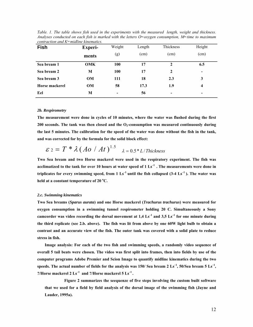
Table. 1. The table shows fish used in the experiments with the measured length, weight and thickness. Analyses conducted on each fish is marked with the letters O=oxygen consumption, M=time to maximum contraction and K=midline kinematics. Fish Experi-
ments
Weight
(g)
Length
(cm)
Thickness
(cm)
Height
(cm)
Sea bream 1 OMK 100 17 2 6.5
Sea bream 2 M 100 17 2 -
Sea bream 3 OM 111 18 2.3 3
Horse mackerel OM 58 17.3 1.9 4
Eel M - 56 - -
2b. Respirometry
The measurement were done in cycles of 10 minutes, where the water was flushed during the first
200 seconds. The tank was then closed and the O2-consumption was measured continuously during
the last 5 minutes. The calibration for the speed of the water was done without the fish in the tank,
and was corrected for by the formula for the solid block effect:
5.12 )/(* AtAoT λε = ThicknessL /*5.0=λ
Two Sea bream and two Horse mackerel were used in the respiratory experiment. The fish was
acclimatized to the tank for over 10 hours at water speed of 1 Ls–1 . The measurements were done in
triplicates for every swimming speed, from 1 Ls–1 until the fish collapsed (3-4 Ls–1 ). The water was
held at a constant temperature of 20 oC.
2.c. Swimming kinematics
Two Sea breams (Sparus aurata) and one Horse mackerel (Trachurus trachurus) were measured for
oxygen consumption in a swimming tunnel respirometer holding 20 C. Simultaneously a Sony
camcorder was video recording the dorsal movement at 1,4 Ls–1 and 3,5 Ls–1 for one minute during
the third replicate (see 2.b. above). The fish was lit from above by one 60W light bulb to obtain a
contrast and an accurate view of the fish. The outer tank was covered with a solid plate to reduce
stress in fish.
Image analysis: For each of the two fish and swimming speeds, a randomly video sequence of
overall 5 tail beats were chosen. The video was first split into frames, then into fields by use of the
computer programs Adobe Premier and Scion Image to quantify midline kinematics during the two
speeds. The actual number of fields for the analysis was 150/ Sea bream 2 Ls–1, 50/Sea bream 5 Ls–1,
?/Horse mackerel 2 Ls–1 and ?/Horse mackerel 5 Ls–1 .
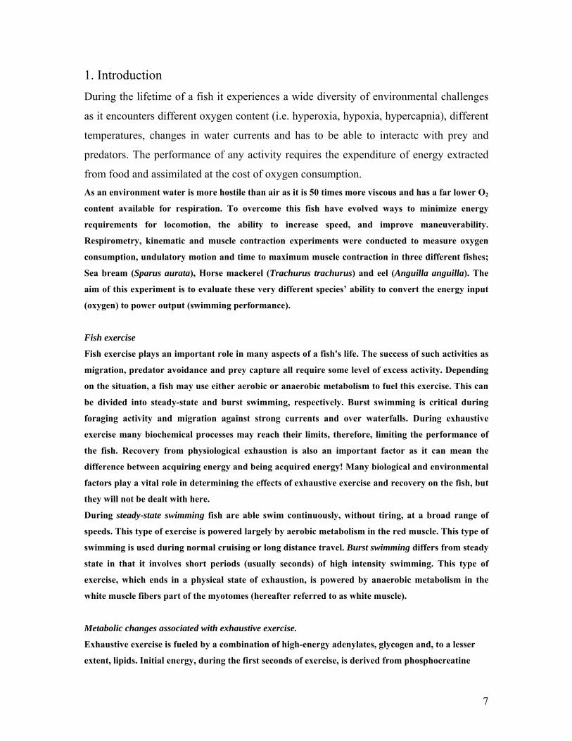
Figure 2 summarizes the seequenze of five steps involving the custom built software
that we used for a field by field analysis of the dorsal image of the swimming fish (Jayne and
Lauder, 1995a).
12
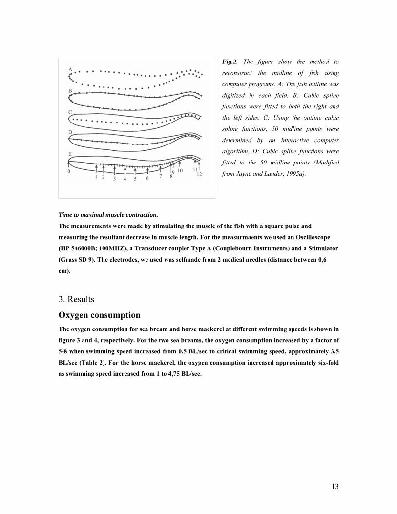
Fig.2. The figure show the method to
reconstruct the midline of fish using
computer programs. A: The fish outline was
digitized in each field. B: Cubic spline
functions were fitted to both the right and
the left sides. C: Using the outline cubic
spline functions, 50 midline points were
determined by an interactive computer
algorithm. D: Cubic spline functions were
fitted to the 50 midline points (Modified
from Jayne and Lauder, 1995a).
Time to maximal muscle contraction.
The measurements were made by stimulating the muscle of the fish with a square pulse and
measuring the resultant decrease in muscle length. For the measurmaents we used an Oscilloscope
(HP 546000B; 100MHZ), a Transducer coupler Type A (Couplebourn Instruments) and a Stimulator
(Grass SD 9). The electrodes, we used was selfmade from 2 medical needles (distance between 0,6
cm).
3. Results
Oxygen consumption The oxygen consumption for sea bream and horse mackerel at different swimming speeds is shown in
figure 3 and 4, respectively. For the two sea breams, the oxygen consumption increased by a factor of
5-8 when swimming speed increased from 0.5 BL/sec to critical swimming speed, approximately 3,5
BL/sec (Table 2). For the horse mackerel, the oxygen consumption increased approximately six-fold
as swimming speed increased from 1 to 4,75 BL/sec.
13

y = 74,643e0,5403x
R2 = 0,9407
y = 92,807e0,638x
R2 = 0,964
0
100
200
300
400
500
600
700
800
900
0 0,5 1 1,5 2 2,5 3 3,5 4
Swimming speed, BL/sec
O2-
Con
sum
ptio
n, m
g/kg
/h
Sea bream 1
Sea bream 3
Figure 3. Oxygen consumption of sea bream at different swimming speeds.
y = 172,38e0,3944x
R2 = 0,9158
0
200
400
600
800
1.000
1.200
1.400
0,0 1,0 2,0 3,0 4,0 5,0
Swimming speed (BL/ sec)
O2-
Con
sum
ptio
n (m
g /k
g/hr
)
Horse mackerel
Figure 4. Oxygen consumption of horse mackerel at different swimming speed
14

The critical swimming speed was higher for the horse mackerel than for the sea breams, as shown in table 2.
This fish was smaller than the two sea breams, and sea bream 3, with the lowest critical swimming speed, was the
largest fish.
Table 2. Critical swimming speed for sea bream and horse mackerel.
Critical swimming speed (BL/sec)
Sea bream 1 3.65
Sea bream 3 3.35
Horse mackerel 4.75
Cost of transport The cost of transport (COT) for the sea breams (fig. 5) was lowest at a swimming speed of approximately two
BL/sec, somewhat lower for seabream 3 (the bigger fish) than for seabream 1. The horse mackerel had the lowest
cost of transport swimming at a speed of three BL/sec (fig. 6).
y = 0,0048x2 - 0,0203x + 0,0525R2 = 0,352
y = 0,018x2 - 0,072x + 0,1112R2 = 0,6059
0
0,02
0,04
0,06
0,08
0,1
0,12
0 0,5 1 1,5 2 2,5 3 3,5 4
Swimming speed, BL/sec
Tota
l cos
t of t
rans
port
(mg
O2
/kg/
BL Sea bream 1
Sea bream 3
Figure 5. Cost of transport for sea bream at different swimming speeds
15

y = 0,0042x2 - 0,0253x + 0,0913R2 = 0,3264
0,000,010,020,030,040,050,060,070,080,09
0 0,5 1 1,5 2 2,5 3 3,5 4 4,5 5Swimming speed (BL/sec)
Tota
l cos
t of t
rans
port
(mg
O2/
kg/B
L)Horse macerel
Figure 6. Cost of transport for horse mackerel at different swimming speeds
Oxygen dept The oxygen consumption of the fish were measured at low swimming speed for some hours after exercising the
fish. The sea breams did not reach as low oxygen consumption levels as at start of the experiments, indicating a
large oxygen dept. Two hours after performing the highest swimming speed, the horse mackerels oxygen
consumption was almost as low as at the start of the experiment (Fig 7, 8 and 9).
0
100
200
300
400
500
600
700
12 14 16 18 20 22
Time (h)
O2-
Con
sum
ptio
n (m
g/kg
/h)
0
0,5
1
1,5
2
2,5
3
3,5
4
Swim
min
g sp
eed
(BL/
sec)
O2-Consumtion, Sea bream 1
Sw imming speed
Fig 7. Oxygen dept in sea bream 1.
16

0
100
200
300
400
500
600
700
800
900
1000
12,00 14,00 16,00 18,00 20,00
Time (h)
O2-
Con
sum
ptio
n (m
g/kg
/h)
0
0,5
1
1,5
2
2,5
3
3,5
4
Swim
min
g sp
eed
(BL/
sec)
O2-Consumption, Sea bream 3
Sw imming speed
Fig 8. Oxygen dept in sea bream 3.
0
200
400
600
800
1000
1200
1400
9:36 12:00 14:24 16:48 19:12Time
Oxy
gen
cons
umpt
ion
(mg/
kg/h
)
0
0,5
1
1,5
2
2,5
3
3,5
4
4,5
5
Swim
min
g sp
eed
(BL/
sec)
Oxygen consumption, Horse mackerelSw imming speed
Fig 9. Oxygen dept in horse mackerel.
17
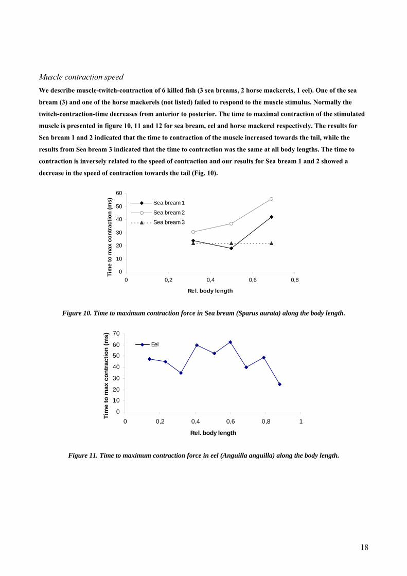
Muscle contraction speed We describe muscle-twitch-contraction of 6 killed fish (3 sea breams, 2 horse mackerels, 1 eel). One of the sea
bream (3) and one of the horse mackerels (not listed) failed to respond to the muscle stimulus. Normally the
twitch-contraction-time decreases from anterior to posterior. The time to maximal contraction of the stimulated
muscle is presented in figure 10, 11 and 12 for sea bream, eel and horse mackerel respectively. The results for
Sea bream 1 and 2 indicated that the time to contraction of the muscle increased towards the tail, while the
results from Sea bream 3 indicated that the time to contraction was the same at all body lengths. The time to
contraction is inversely related to the speed of contraction and our results for Sea bream 1 and 2 showed a
decrease in the speed of contraction towards the tail (Fig. 10).
0
10
20
30
40
50
60
0 0,2 0,4 0,6 0,8
Rel. body length
Tim
e to
max
con
trac
tion
(ms) Sea bream 1
Sea bream 2
Sea bream 3
Figure 10. Time to maximum contraction force in Sea bream (Sparus aurata) along the body length.
0
10
20
30
40
50
60
70
0 0,2 0,4 0,6 0,8 1
Rel. body length
Tim
e to
max
con
trac
tion
(ms)
Eel
Figure 11. Time to maximum contraction force in eel (Anguilla anguilla) along the body length.
18

0
5
10
15
20
25
30
0,2 0,3 0,4 0,5 0,6 0,7
Rel. body length
Tim
e to
max
con
trac
tion
(ms) Horse mackerel
Figure 12 . Time to maximum contraction force Horse mackerel ( )along the body length
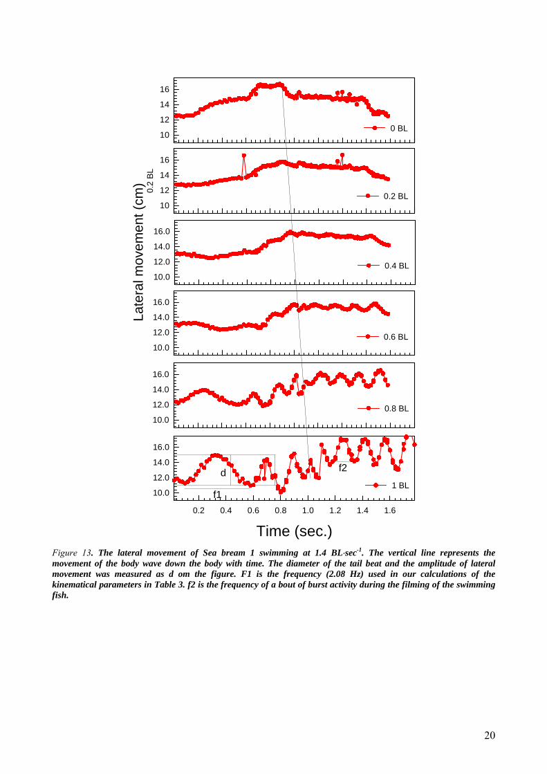
Kinematics The kinematics of Sea bream 1 swimming at 1.4 BL⋅sec-1 and 3.5 BL⋅sec-1is shown in Figure 13 and 14,
respectively. The progression of the body wave down the fish’s body is indicated in figure 13. In the last part of
the figure the frequency and amplitude of the body wave are indicated. At 3.5 BL⋅sec-1 the movement of the fish’s
is almost exclusively but the back half of the body (Figure 14).
Table 3 lists the kinematical parameters that we calculated from the swimming Sea bream. As swimming speed
increased from 1.4 BL⋅sec-1 the frequency of tail beats increased from 2.08 Hz to 4.78 Hz, the increase came
about without an equally sized decrease in amplitude of the body wave traveling down the fish (Table 3, Fig 13
and 14). The thrust power increased from 2.8 mWatts to 37 mWatts as swimming velocity increased, and thus
mirrored the increase in the total power of the fish, as the kinematically lost power increased less (Table 3). The
Froude efficiency decreased at higher swimming velocities and indicates that the efficiency of turning the power
of the wave traveling down the body into propulsion, i.e. thrust power or swimming velocity, decreased. The total
efficiency of converting the consumed power (oxygen) into thrust power increased at higher swimming velocity.
19
10
12
14
16
0 BL
10
12
14
160.
2BL
0.2 BL
10.0
12.0
14.0
16.0
Late
ralm
ovem
ent(
cm)
0.4 BL
10.0
12.0
14.0
16.0
0.6 BL
10.0
12.0
14.0
16.0
0.8 BL
10.0
12.0
14.0
16.0
0.2 0.4 0.6 0.8 1.0 1.2 1.4 1.6
Time (sec.)
1 BLd
f1
f2
Figure 13. The lateral movement of Sea bream 1 swimming at 1.4 BL⋅sec-1. The vertical line represents the movement of the body wave down the body with time. The diameter of the tail beat and the amplitude of lateral movement was measured as d om the figure. F1 is the frequency (2.08 Hz) used in our calculations of the kinematical parameters in Table 3. f2 is the frequency of a bout of burst activity during the filming of the swimming fish.
20

bl 0
05
101520253035
00.0
40.0
80.1
20.1
6 0.2 0.24
0.28
0.32
0.36 0.4 0.4
40.4
80.5
20.5
6 0.6 0.64
0.68
0.72
0.76 0.8 0.8
40.8
80.9
20.9
61.0
01.0
41.0
81.1
21.1
61.2
01.2
41.2
81.3
21.3
61.4
0
bl 0
bl 0.2
0
5
10
15
20
25
30
0
0.04
0.08
0.12
0.16 0.2
0.24
0.28
0.32
0.36 0.4
0.44
0.48
0.52
0.56 0.6
0.64
0.68
0.72
0.76 0.8
0.84
0.88
0.92
0.96
1.00
1.04
1.08
1.12
1.16
1.20
1.24
1.28
1.32
1.36
1.40
bl 0.2
bl 0.4
0
5
10
15
20
25
30
0
0.04
0.08
0.12
0.16 0.2
0.24
0.28
0.32
0.36 0.4
0.44
0.48
0.52
0.56 0.6
0.64
0.68
0.72
0.76 0.8
0.84
0.88
0.92
0.96
1.00
1.04
1.08
1.12
1.16
1.20
1.24
1.28
1.32
1.36
1.40
bl 0.4
bl 0.6
05
1015202530
00.0
40.0
80.1
20.1
6 0.2 0.24
0.28
0.32
0.36 0.4 0.4
40.4
80.5
20.5
6 0.6 0.64
0.68
0.72
0.76 0.8 0.8
40.8
80.9
20.9
61.0
01.0
41.0
81.1
21.1
61.2
01.2
41.2
81.3
21.3
61.4
0
bl 0.6
bl 0.8
0
5
10
15
20
25
0
0.04
0.08
0.12
0.16 0.2
0.24
0.28
0.32
0.36 0.4
0.44
0.48
0.52
0.56 0.6
0.64
0.68
0.72
0.76 0.8
0.84
0.88
0.92
0.96
1.00
1.04
1.08
1.12
1.16
1.20
1.24
1.28
1.32
1.36
1.40
bl 0.8
1.0 bl
0
5
10
15
20
0
0.04
0.08
0.12
0.16 0.2
0.24
0.28
0.32
0.36 0.4
0.44
0.48
0.52
0.56 0.6
0.64
0.68
0.72
0.76 0.8
0.84
0.88
0.92
0.96
1.00
1.04
1.08
1.12
1.16
1.20
1.24
1.28
1.32
1.36
1.40
1.0 bl
Figure 13. The lateral movement of Sea bream 1 swimming at 3.5 BL⋅sec-1
Table 3. The kinematical parameters determined from one swimming Sea bream
Species Length Weight Swimming
velocity wave velocity freq. Amplitude Ptot Pke Pt Efficiency Froude eff.
21
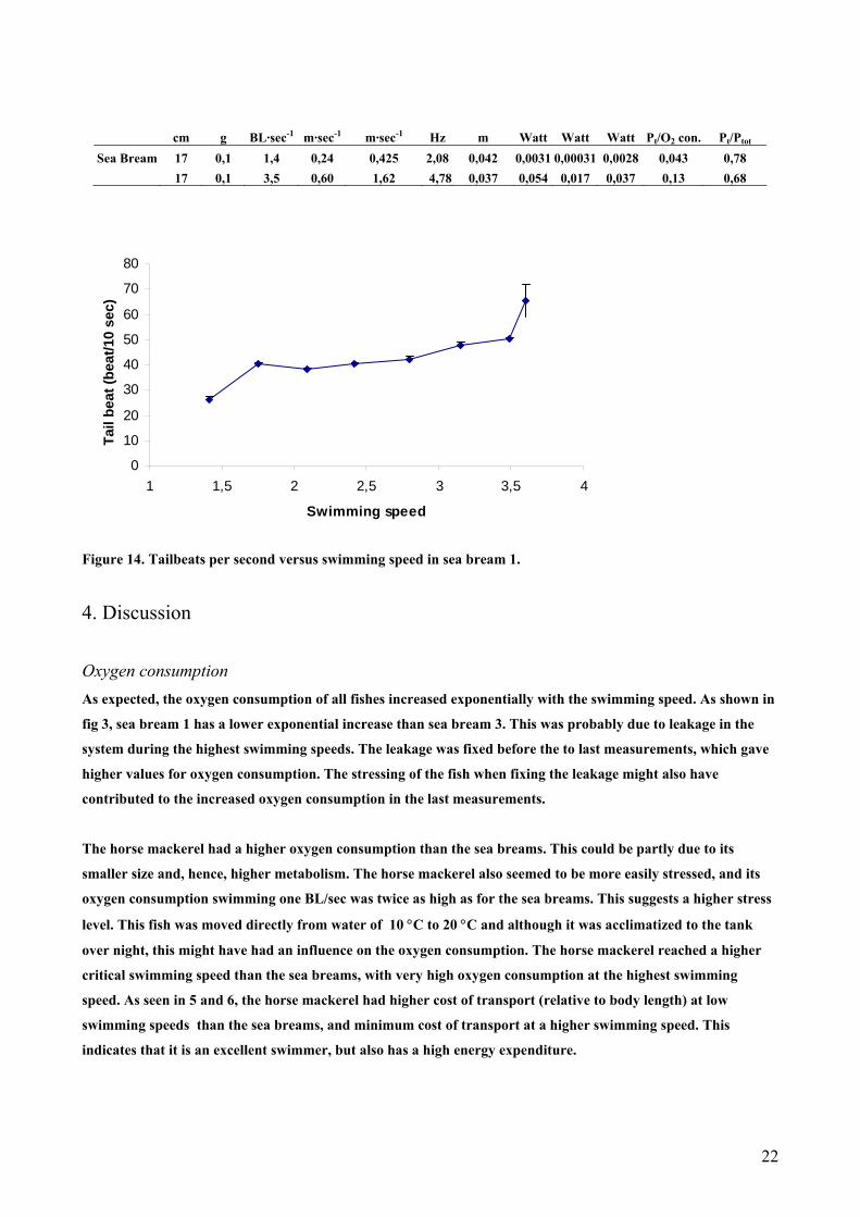
cm g BL·sec-1 m·sec-1 m·sec-1 Hz m Watt Watt Watt Pt/O2 con. Pt/Ptot
Sea Bream 17 0,1 1,4 0,24 0,425 2,08 0,042 0,0031 0,00031 0,0028 0,043 0,78 17 0,1 3,5 0,60 1,62 4,78 0,037 0,054 0,017 0,037 0,13 0,68
0
10
20
30
40
50
60
70
80
1 1,5 2 2,5 3 3,5 4
Swimming speed
Tail
beat
(bea
t/10
sec)
Figure 14. Tailbeats per second versus swimming speed in sea bream 1.
4. Discussion
Oxygen consumption As expected, the oxygen consumption of all fishes increased exponentially with the swimming speed. As shown in
fig 3, sea bream 1 has a lower exponential increase than sea bream 3. This was probably due to leakage in the
system during the highest swimming speeds. The leakage was fixed before the to last measurements, which gave
higher values for oxygen consumption. The stressing of the fish when fixing the leakage might also have
contributed to the increased oxygen consumption in the last measurements.
The horse mackerel had a higher oxygen consumption than the sea breams. This could be partly due to its
smaller size and, hence, higher metabolism. The horse mackerel also seemed to be more easily stressed, and its
oxygen consumption swimming one BL/sec was twice as high as for the sea breams. This suggests a higher stress
level. This fish was moved directly from water of 10 °C to 20 °C and although it was acclimatized to the tank
over night, this might have had an influence on the oxygen consumption. The horse mackerel reached a higher
critical swimming speed than the sea breams, with very high oxygen consumption at the highest swimming
speed. As seen in 5 and 6, the horse mackerel had higher cost of transport (relative to body length) at low
swimming speeds than the sea breams, and minimum cost of transport at a higher swimming speed. This
indicates that it is an excellent swimmer, but also has a high energy expenditure.
22

The horse mackerel also recovered faster from the oxygen dept than the sea breams, which did not recover from
the oxygen dept while the measurements were performed.
The high oxygen dept of the sea breams indicates large capacity for anaerobic activity. The high oxygen
consumption and fast recovery from oxygen dept in the horse mackerel indicates a high capacity for oxygen
transport and extraction in this species.
Swimming kinematics The Sea bream appears to be a very efficient swimmer based on our results (Table 3). A a swimming speed of 1.4
BL·sec-1 it has an efficiency of 4.3% in turning the consumed oxygen into muscle thrust exerted on the water.
This is less than the the efficiency found in the chub mackerel (Scomber japonicus) (Shadwick and Steffensen, P
2.68), which has an efficiency of 6.5% when swimming at 1.4 BL·sec-1, which increases to 10% at 3.5 BL·sec-1. At
higher swimming speed ( 3.5 BL·sec-1) the Sea bream convert the oxygen input to power output with an efficiency
of 13%, which is higher than that measured for chub mackerel (Shadwick and Steffensen, P 2.68). The increase
in efficiency of converting ingested power into thrust probably indicates a shift in the amount of energy being
used to assimilate food, reproduce, and other energy consuming processes.
The Froude efficiency expresses the efficiency by which the fish converts the energy of the wave progressing
down the body to swimming velocity. The velocity of the progressing undulatory wave is higher than the
swimming velocity, but the more similar they are, the more efficient do the fish convert the energy in the
progressing wave to swimming energy or thrust power. The Froude efficiency of the Sea bream is 78% and 68%
when swimming at 1.4 and 3.5 BL·sec-1, respectively. These efficiencies are similar to those seen in the chub
mackerel, which has a Froude efficiency of 80 % irrespectively of swimming velocity (Shadwick and Steffensen,
P 2.68).
The frequency of tail beats increases as the swimming velocity increases from around 2 Hz at 1.4 BL·sec-1 to 4.8
Hz at 3.5 BL·sec-1. This occurs concomitantly with an increase in the velocity of the wave progressing down the
body, and since the relationship between the wave velocity and the frequency is: fc λ= , this means that the
wavelength increases from 20,4 cm to 33.8 cm when swimming velocity increases from 1.4 to 3.5 BL·sec-1 (fig. 13
and 14). As evident from Figure 13 and 14 the increase in tail beat frequency brings about a decrease in the
amplitude of a tail beat at both 1.4 abd 3.5 BL·sec-1 (table M).
Muscle contraction speed The method used to measure the time to maximal muscle contraction was developed by R.E. Shadwick and
colleagues. It provides an indication of how fast the muscle contracts at different body lengths, and is thus an
indication of how the timing of the stimulus of the muscles should be in a live, swimming fish. Our results
indicate that the timing of the muscle stimulation occurs somewhat later at more posterior body lengths than at
the anterior. The eel apparently has a more complicated timing of its muscle stimulus as indicates by the shape of
the curve showing the time to maximal contraction (Fig. 11). At the most anterior location of measurement the
23

time to contraction is lower than further back, while at the most posterior locations the time to contraction is
again shorter.
The data for the Sea breams and the horse mackerel give different results if the above interpretation is valid. In
the Sea bream the time to maximal contraction increases toward the posterior, while in the horse mackerel the
opposite trend is seen. According to a reliable source (R.E. Shadwick) normally the time to maximal contraction
increases towards the posterior, and this is consistent with our results where the horse mackerel was a poor test
subject, and the data from it are probably not very good. If the time to maximal contraction is an indication of
the time it takes a live, swimming fish to contract the swimming muscles then our results from the sea breams
are in accordance with data reviewed by Altringham and Ellerby (1999) for several different species of fish.
These authors find a linear increase in the contraction times along the length of the body.
5. References
Altringham, J.D., and Ellerby, D.J. (1999) Fish swimming: patterns in muscle function. J. exp.Biol. 202: 3397-
3403.
Jayne, Bruce C. and Lauder George V. (1995a). Speed effect on midline kinematics during steady undulatory
swimming of largemouth bass, Micropterus salmoides. J. exp. Biol. 198: 585-602.
Jayne, Bruce C. and Lauder George V. (1995a). Speed effect on midline kinematics during steady undulatory
swimming of largemouth bass, Micropterus salmoides. J. exp. Biol. 198: 585-602.
Webb, P.W., Kostecki, P.T., and Stevens, E.D. (1984) The effect of size and swimming speed on locomotor
kinematics of rainbow trout. J. exp. Biol. 109: 77-95.
Shadwick, R.E., and Steffensen, J.F. The cost and efficiency of locomotion in the chub mackerel, Scomber
japonicus. P 2.68.
Steffensen, J.F., Johansen, K., and Bushnell, P.G. (1984) An automated swimming respirometer.
24

7. Appendix Information on the fish species used in our experiments:
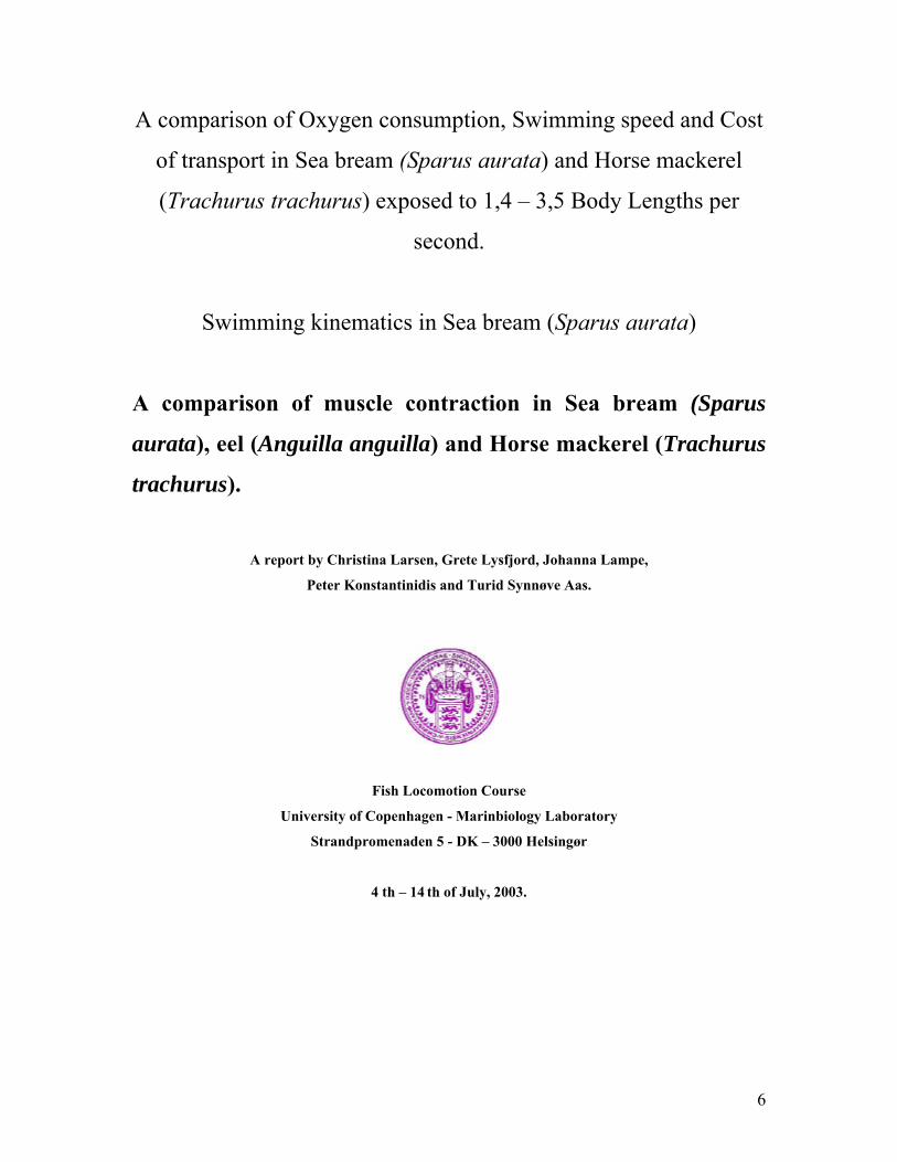
Gilthead seabream (Sparus aurata)
Fig.?: Giltheatd seabream (Sparus aurata).
(http://www.fishbase.org/Photos/PicturesSummary.cfm?StartRow=4&ID=1164&what=species, 2003).
The Gilthead seabream belong to the family Sparidae, witch are chiefly marine and very rare in fresh- and
brackish water. The distribution are tropical and temperate Atlantic, Indian and Pacific Oceans. Many species
have been found to be hermaphroditic; some have male and female gonads simultaneously; others change sex as
they get larger. Maximum size are reported to be 70.0 cm and maximum weight: 17.2 kg. Maximum reported
age are 11 years. It lives demersal in freshwater, brackish and marine waters within depth range 1 - 150 m. Its’s
distribution are subtropical (57°N - 43°S), eastern Atlantic with British Isles, Straits of Gibraltar to Cape
Verde and around the Canary Islands and the Mediterranean. The sea bream inhabits seagrass beds and sandy
bottoms as well as in the surf zone commonly to depths of about 30 m, but adults may occur to 150 m depth. It’s
a sedentary fish, either solitary or in small aggregations. Mainly carnivorous, accessorily herbivorous. The
Gilthead seabream feeds on shellfish, including mussels and oysters, and it’s mainly carnivorous, accessorily
herbivorous. One of the most important fishes in saline and hypersaline aquaculture.
Horse mackerel (Trachurus trachurus)
25
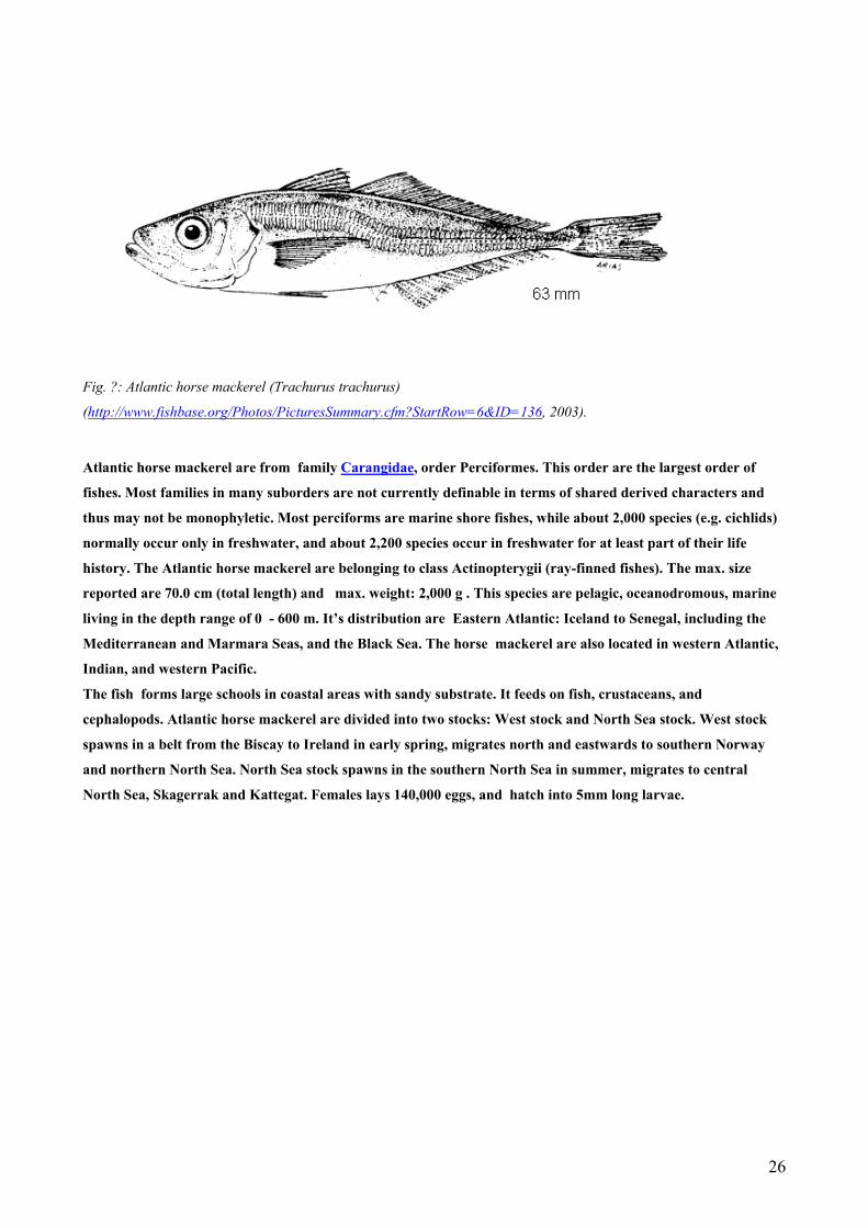
Fig. ?: Atlantic horse mackerel (Trachurus trachurus)
(http://www.fishbase.org/Photos/PicturesSummary.cfm?StartRow=6&ID=136, 2003).
Atlantic horse mackerel are from family Carangidae, order Perciformes. This order are the largest order of
fishes. Most families in many suborders are not currently definable in terms of shared derived characters and
thus may not be monophyletic. Most perciforms are marine shore fishes, while about 2,000 species (e.g. cichlids)
normally occur only in freshwater, and about 2,200 species occur in freshwater for at least part of their life
history. The Atlantic horse mackerel are belonging to class Actinopterygii (ray-finned fishes). The max. size
reported are 70.0 cm (total length) and max. weight: 2,000 g . This species are pelagic, oceanodromous, marine
living in the depth range of 0 - 600 m. It’s distribution are Eastern Atlantic: Iceland to Senegal, including the
Mediterranean and Marmara Seas, and the Black Sea. The horse mackerel are also located in western Atlantic,
Indian, and western Pacific.
The fish forms large schools in coastal areas with sandy substrate. It feeds on fish, crustaceans, and
cephalopods. Atlantic horse mackerel are divided into two stocks: West stock and North Sea stock. West stock
spawns in a belt from the Biscay to Ireland in early spring, migrates north and eastwards to southern Norway
and northern North Sea. North Sea stock spawns in the southern North Sea in summer, migrates to central
North Sea, Skagerrak and Kattegat. Females lays 140,000 eggs, and hatch into 5mm long larvae.
26
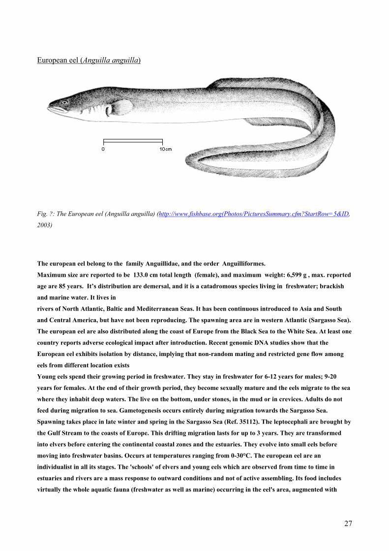
European eel (Anguilla anguilla)
Fig. ?: The European eel (Anguilla anguilla) (http://www.fishbase.org(Photos/PicturesSummary.cfm?StartRow=5&ID,
2003)
The european eel belong to the family Anguillidae, and the order Anguilliformes.
Maximum size are reported to be 133.0 cm total length (female), and maximum weight: 6,599 g , max. reported
age are 85 years. It’s distribution are demersal, and it is a catadromous species living in freshwater; brackish
and marine water. It lives in
rivers of North Atlantic, Baltic and Mediterranean Seas. It has been continuous introduced to Asia and South
and Central America, but have not been reproducing. The spawning area are in western Atlantic (Sargasso Sea).
The european eel are also distributed along the coast of Europe from the Black Sea to the White Sea. At least one
country reports adverse ecological impact after introduction. Recent genomic DNA studies show that the
European eel exhibits isolation by distance, implying that non-random mating and restricted gene flow among
eels from different location exists
Young eels spend their growing period in freshwater. They stay in freshwater for 6-12 years for males; 9-20
years for females. At the end of their growth period, they become sexually mature and the eels migrate to the sea
where they inhabit deep waters. The live on the bottom, under stones, in the mud or in crevices. Adults do not
feed during migration to sea. Gametogenesis occurs entirely during migration towards the Sargasso Sea.
Spawning takes place in late winter and spring in the Sargasso Sea (Ref. 35112). The leptocephali are brought by
the Gulf Stream to the coasts of Europe. This drifting migration lasts for up to 3 years. They are transformed
into elvers before entering the continental coastal zones and the estuaries. They evolve into small eels before
moving into freshwater basins. Occurs at temperatures ranging from 0-30°C. The european eel are an
individualist in all its stages. The 'schools' of elvers and young eels which are observed from time to time in
estuaries and rivers are a mass response to outward conditions and not of active assembling. Its food includes
virtually the whole aquatic fauna (freshwater as well as marine) occurring in the eel's area, augmented with
27

animals living out of water, e.g. worms. At an age of 6-30 years, eels begin to undergo a remarkable series of
changes, eyes are enlarged, head becomes pointed, skin on the back darker, while that on the belly becomes shiny
and silvery. Best temperature for making eels sexually mature is 20-25°C.
Appendix 2 Video analysis instruction Version 1. Use Scion Image to digitize sequential video fields. Bottom left corner of screen should be set as origin (0,0). Things to adjust before you start digitizing:
Under Options Preferences: click Invert y coordinates
Under Analyze Options: click X-Y center and change Max Measurements to 8000.
To the output file (Excel) that results from digitizing in Scion Image, multiply all x values (left column) by –1 to make sure that the anterior of the fish corresponds to the lowest X coordinates. Do this only if your fish is oriented such that its tail is near the left side of the screen. To format X-Y coordinate data for entry into Lauder FISH program: Save Excel file containing scion image coordinate data as formatted text (space deliminated). Rename suffix of data file to txt or dat. Note, you will need to use Data Rearranger program to reformat the data ina form that can be recognized by the Lauder FISH program. This Rearranger program can only handle 50 fields at a time, so if you have digitized more than 50 fields you will need to separate the data into multiple files. Open Data Rearranger program and input data file with appropriate extension in quotes. All output files (there will be more than 1 if you digitized more than 50 fields) will be names IFILE. Every time you run Data Rearranger program, you will need to adjust the name of the output file to reflect the set of fields that you have rearranged. Open all Rearranger output IFILEs in Excel and combine (in the correct order) into one big Excel file. Save this file as Formatted text (space delimited). Change suffix from prn to tbl once file is saved. Note, all files should be kept in same folder as that containing the Rearranger and Lauder FISH program. Running Lauder FISH program: Open program. Things to adjust or enter before running program: Enter input file (.tbl suffix) Read 2 rows (analyze midline) MTV starting row = 1 Pause between graphics = Y # Outline points per splice = 4 # midline points = 50 # midline points per splice = 4 % file = percent
Enter your segment angles output file (name it what you want, it will have .ANG suffix) Rearrange .ANG FISH output file using Swim 3 macro. To do this, open both your .ANG file and the macro in Excel, then run the macro. This macro will rearrange the data so that 0’s indicate X coordinates (in cm) of dorsal midline segment points, 1’s indicate Y coordinates (cm), and 2’s indicate dorsal midline segment angles. The angle of each segment along the midline subtended to the segment directly anterior to it. Version 2. How to plot the fish’ midline etc.
1. In adobe premier :
28
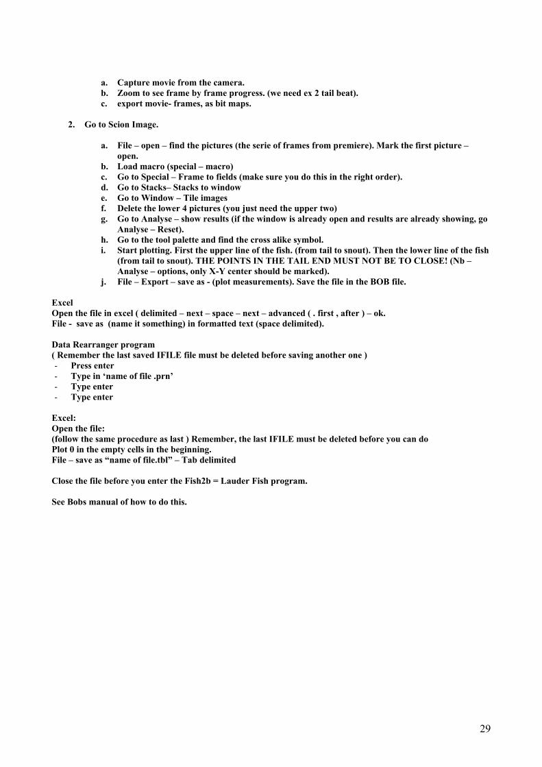
a. Capture movie from the camera. b. Zoom to see frame by frame progress. (we need ex 2 tail beat). c. export movie- frames, as bit maps.
2. Go to Scion Image.
a. File – open – find the pictures (the serie of frames from premiere). Mark the first picture –
open. b. Load macro (special – macro) c. Go to Special – Frame to fields (make sure you do this in the right order). d. Go to Stacks– Stacks to window e. Go to Window – Tile images f. Delete the lower 4 pictures (you just need the upper two) g. Go to Analyse – show results (if the window is already open and results are already showing, go
Analyse – Reset). h. Go to the tool palette and find the cross alike symbol. i. Start plotting. First the upper line of the fish. (from tail to snout). Then the lower line of the fish
(from tail to snout). THE POINTS IN THE TAIL END MUST NOT BE TO CLOSE! (Nb – Analyse – options, only X-Y center should be marked).
j. File – Export – save as - (plot measurements). Save the file in the BOB file. Excel Open the file in excel ( delimited – next – space – next – advanced ( . first , after ) – ok. File - save as (name it something) in formatted text (space delimited). Data Rearranger program ( Remember the last saved IFILE file must be deleted before saving another one ) - Press enter - Type in ‘name of file .prn’ - Type enter - Type enter
Excel: Open the file: (follow the same procedure as last ) Remember, the last IFILE must be deleted before you can do Plot 0 in the empty cells in the beginning. File – save as “name of file.tbl” – Tab delimited Close the file before you enter the Fish2b = Lauder Fish program. See Bobs manual of how to do this.
29

Electrophysiological monitoring in fish: Examinations of the European eel (Anguilla anguilla) and the Atlantic cod
(Gadus morhua)
A project carried out under the auspices of the SLIP PhD course Biomechanics, bioenergetics and physiology of swimming fish.
By Maria Faldborg Petersen, Dr. Neill A. Herbert, and Paul Maslen Electrophysiological monitoring in fish
30

General Introduction Measurements of the rate at which fish consume oxygen (VO2) within their natural environment allow estimation of gross energy transfer, the energetic-cost of short term behaviours and the temporal allocation of metabolic scope to various activities (such as digestion, reproduction etc)(Armstrong, 1998). Given that an improved understanding of metabolic allocations within wild populations would greatly advance the resolution of bioenergetic models various electrophysiological tools have been developed to estimate fish VO2. Total fish metabolism is comprised of 3 components (standard, active and feeding metabolism) and can be measured in the field using a variety of electrophysiological tools that are typically coupled with remote telemetric devices. It is theoretically possible to measure active metabolism by measuring electromyogram (EMG) signals (as a correlate of activity in the opercular and/or trunk musculature) and deriving an energetic unit from laboratory-based activity vs. VO2 relations (Briggs and Post, 1997; Økland et al. 1997). It is also theoretically possible to estimate standard, active and feeding rates of metabolism from electrocardiogram (ECG) signals that correlate heart rate frequency with VO2 (Armstrong, 1998). However, the degree to which all these electrophysiological signals correlate with VO2 (and hence their usefulness in field-based estimates) is still open to debate. The aim of the Electrophysiological section of the MBL Fish Physiology Course is twofold: 1) address the nature of electrophysiological-metabolic relations in 2 species of fish; the Atlantic cod, Gadus morhua, and the European eel, Anguilla anguilla, and 2) to assess the biological and technological limitations of using EMGs and ECGs for in vivo, field-based monitoring.
31
Do electromyograms correlate with oxygen consumption and lateral body displacement?
Introduction The generation of different types of movement by fish is dependent on the type,
amount and positioning of various types of muscle. Fish muscle typically consists of two
fibre types: 1) Red (“slow twitch”) fibres are often located as a narrow wedge along the
length of the septum and are employed for steady (aerobic) swimming, 2) white “fast
twitch” fibres comprise the bulk of the axial musculature and are activated for intense burst
(anaerobic) activities. Although the amount and positioning of these different fibres is
important for fish swimming, the generation of power is ultimately controlled by their
sequential activation along the length of the body. Given that the amplitude of lateral tail
displacement increases along the length of the body it is highly likely that the timing of
EMG signals will also vary according to their position along the body (Beddow and
McKinley, 1999).
The aim of the current project was to examine whether EMG signals and the
amount of lateral tail displacement was correlated with electrode positioning, as well as
VO2 at different swimming speeds, in two species of fish (A. anguilla and G. morhua).
These species were selected because their swimming gaits contrast markedly (i.e.
anguilliform vs. subcarangiform) and their fibre type distributions are different. The amount
of red fibres was found to be very low in both species, however, it was found as a uniform
but thin superficial band along the entire length of the eel and as an indiscrete (septal)
wedge in the cod. Therefore, we would expect significant differences in the EMG signals of
the 2 species with position along the body (i.e. larger differences within the subcarangiform
swimmer).
Materials and Methods The EMGs and lateral body displacement of 2 cod (FL= 25-30cm) and 2 eel (FL =
30-35 cm) was assessed whilst swimming within a 31.45 L respirometer at various speeds
(0.35, 0.75 and 1.1 BL/s).
EMG electrodes were implanted after fish were anaesthetised with Benzocaine (10
mg/L). Two fine wire electrodes with a 1 mm bent exposed tip were inserted into the red
32
(slow twitch) and white (fast twitch) muscle fibres at various points along the body of the
eel and cod (0.5 and 0.75 BL) and attached securely with sutures and 3M Vetbond
adhesive. EMG signals were initially transferred to an RM systems differential AC
amplifier, equipped with low and high pass filters, followed by a Hewlett Packard 54600B
100 MHz oscilloscope and finally stored on a portable PC after further digital filtering
(Acknowledge).
Fish were placed into the swimming respirometer and initial water flow was
maintained at a constant speed of 0.35 BL/s. To monitor the effect of increasing swimming
speed on the physical lateral displacements of the body, a 0.5 x 0.5 cm piece of 3M
reflective tape “marker” was adhered to the dorsal surface of the fish at the same positions
as EMG electrodes (i.e. 0.5 and 0.75 FL). A white LED was positioned directly above the
fish and ensured that the “marker” was satisfactorily illuminated. Moving images were
recorded on a Hitachi Hi8 camcorder and transferred to a computer equipped with a frame
grabber (Visionetics VFG-512 BC) that digitizes single video frames with a resolution of
256 x 256 pixels at 10 frames s-1. The x-y coordinates of the “marker” was determined and
transmitted via the RS-232 port to a data acquisition package (Labtech Notebook). X, y
data was stored on the hard drive for later calculations of lateral displacement vs. time.
Rates of oxygen consumption were measured by the rate of PO2 decrease within
the respirometer over a 5 minute period according to Schurmann and Steffensen (1997).
Results and discussion
White muscle EMG signals were observed from a single cod (held in a bucket
during preliminary testing) but no clear EMG signals, from either the white or red muscle,
were observed after fish were placed in the respirometer. It is likely that white muscle
fibres were not activated in the respirometer because fish would not swim at speeds
exceeding 0.35 BL/s (i.e. at speeds sufficiently high for white muscle activation).
Surprisingly, red muscle EMGs were not observed at the minimal cruising speed even
though slow caudal contractions were observed. However, we strongly suspect that our
red muscle electrodes were not satisfactorily positioned in the red fibre regions. Given that
the regions in which the red fibres are present are so small in both the cod and eel we
suggest that this methodology may not be optimal for either of these species (at least with
33
specimens less than 40 cm BL). However, red muscle EMGs have been measured
successfully in eel of a similar size (Gillis, 1998) suggesting that we may have experienced
experimental difficulties in terms of satisfactory signal acquisition (e.g. pole reversal!)
and/or filtering.
The lack of well-developed red musculature may be related to the behavioural
lifestyle of these species, given that burst activity is far more prevalent than constant
cruising. We suggest that studies examining red muscle EMGs should only continue with
species known to have well developed regions of red musculature (e.g carangids,
scombrids, salmonids) if an energetic link between free swimming activity and VO2 is
required for bioenergetic modelling.
Given the reluctance of fish to swim, estimated values of VO2 and body lateral
displacements could not be analysed with respect to EMG signals.
A foreseeable limitation of using EMG monitoring with free swimming fish is that
routine activities are rarely linear over prolonged periods and hence EMG signals may be
limited in their ability to represent true activity levels. Although the EMG signals of linearly
swimming fish could be calibrated with VO2 at different swimming speeds in the lab it may
be extremely difficult to equate such signals to activity levels in the wild. Either white and
red muscle EMGs should be used together or, when red muscle fibre levels are low (e.g. in
gadoid species), physiological sensors that measure caudal differential pressures should
probably be used.
34

Heart rate and ventilation frequency as predictors of oxygen consumption in Atlantic cod
during hypoxia
Introduction
Fish may regulate cardiac output and ventilation when oxygen demands increase (i.e. during activity, stress, temperature increase, digestion, hypoxia etc). The mechanisms involved in raising total ventilation include an increase in breathing frequency as well as breath volume. In a similar manner, cardiac output can be increased by a rise in heart rate and/or stroke volume. In both cases the extraction of oxygen, and the efficiency to which this occurs, is subject to change. The strategy by which one or the other cardio-ventilatory parameter is regulated appears to depend on the cause of increased O2 demand. Whilst an increase in temperature appears to increase ventilation by increasing both frequency and volume, the stimulatory effect of temperature on cardiac output is due to an increase in heart rate rather than stroke volume (Randall, 1970). In contrast, aquatic hypoxia increases total ventilation with an increase in breath volume (Steffensen 1982) and an more or less constant cardiac output with a drop in heart rate (termed bradycardia) but increased stroke volume. A reduction in heart rate at a time when hypoxic demands for oxygen increase may seem nonsensical but a slowing of the heart rate actually ensures a constant rate of O2 extraction by prolonging the time for gaseous diffusion across the gill lamellae and capillary networks. Whether there is a coupling between heart rate and ventilation has been widely discussed in the literature. Randall (1970) describes that the level of vagal tone to the heart oscillates in phase with the breathing cycle and tends to inhibit the heart as the mouths opens. This coordinated action should ensure an optimal (synchronous) flow of blood and water at the gills, but since ventilation rate is often higher than heart rate (Laitinen & Valtonen 1994, McKenzie et al. 1995) a coupling between the two parameters is unlikely. Newer literature seems to favour that cardiorespiratory synchronicity is absent (Taylor, 1992). The aim of the present study was to test if heart rate and ventilation frequency can be used to predict oxygen consumption of Atlantic cod during hypoxia.
Materials and methods Atlantic cod (Gadus morhua) were anaesthetised with Benzocaine (10mg/l). Two stainless steel electrodes with a 1mm exposed bent tip were then laterally inserted 2 cm apart into the pericardial
35
cavity and sutured in place at entry point. The electrodes were then sutured on either side of the fish behind the buccal fin, then gathered and sutured together behind the first dorsal fin. The fish was then placed in a swimming respirometer, and the electrodes attached to an A.M. Systems differential AC amplifier and from there to a Hewlett Packard 54600B 100 MHz oscilloscope. The signal was then run through a Biopac MP100 unit and the signal then transferred to a laptop and observed and recorded in Acknowledge 3.7.2. Ventilation rate could be read from the original signal while the signal was filtered through a digital band pass filter to allow observations of the ECG signal. The fish was not swimming in the swimming respirometer, but the water flow was kept at a constant speed of 0.2.BLsec-1 to ensure sufficient water replacement in the respirometer and temperature was
kept constant at 12°C. Oxygen consumption of the fish was measured with a Cameron electrode by
following the decrease of oxygen during a five-minute period. The oxygen level was lowered from 150 mm Hg (94% saturation) to 56 mmHg (35% saturation) by bubbling nitrogen during a period of 4.5 hours. Measurements of heart rate, ventilation rate, oxygen consumption and pO2 in water were measured every 10 minutes.
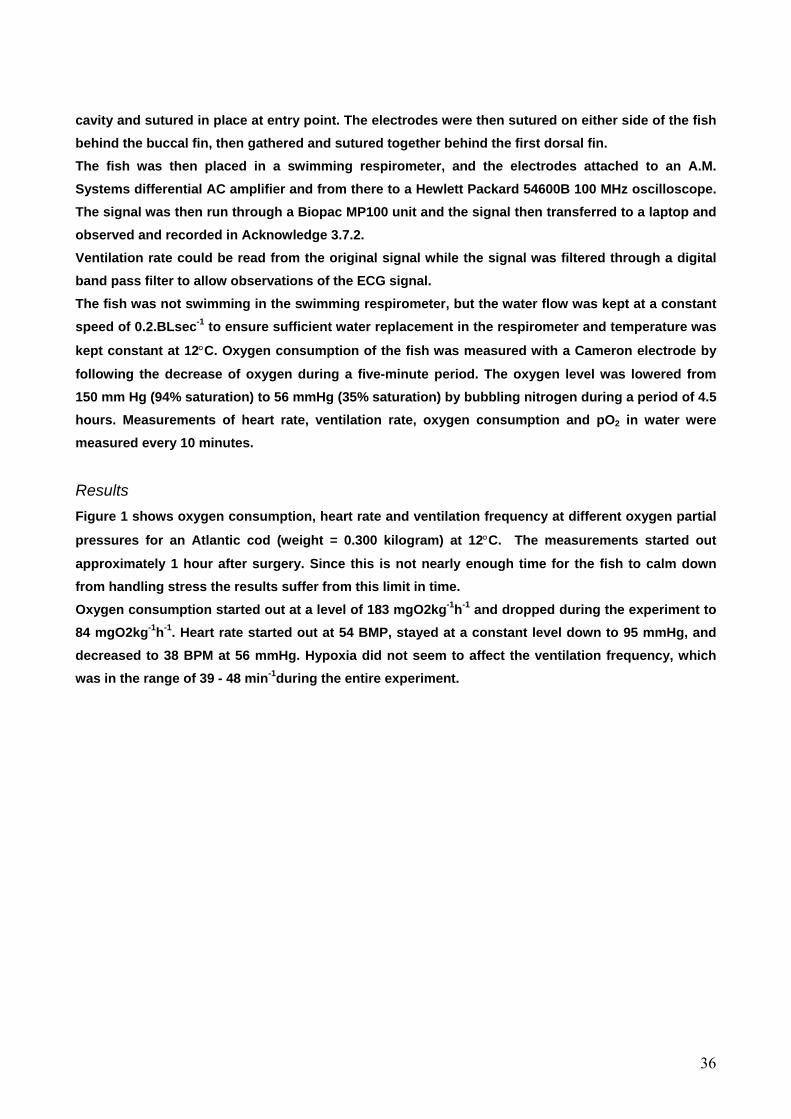
Results Figure 1 shows oxygen consumption, heart rate and ventilation frequency at different oxygen partial
pressures for an Atlantic cod (weight = 0.300 kilogram) at 12°C. The measurements started out
approximately 1 hour after surgery. Since this is not nearly enough time for the fish to calm down from handling stress the results suffer from this limit in time. Oxygen consumption started out at a level of 183 mgO2kg-1h-1 and dropped during the experiment to 84 mgO2kg-1h-1. Heart rate started out at 54 BMP, stayed at a constant level down to 95 mmHg, and decreased to 38 BPM at 56 mmHg. Hypoxia did not seem to affect the ventilation frequency, which was in the range of 39 - 48 min-1during the entire experiment.
36
80
100
120
140
160
180
200
50 70 90 110 130 150pO2 (mmHg)
Oxy
gen
cons
umpt
ion
(mgO
2/kg
/h)
10
20
30
40
50
60
70
HR
and
ven
tilat
ion
freq
(1/m
in)
VO2VentilationHR
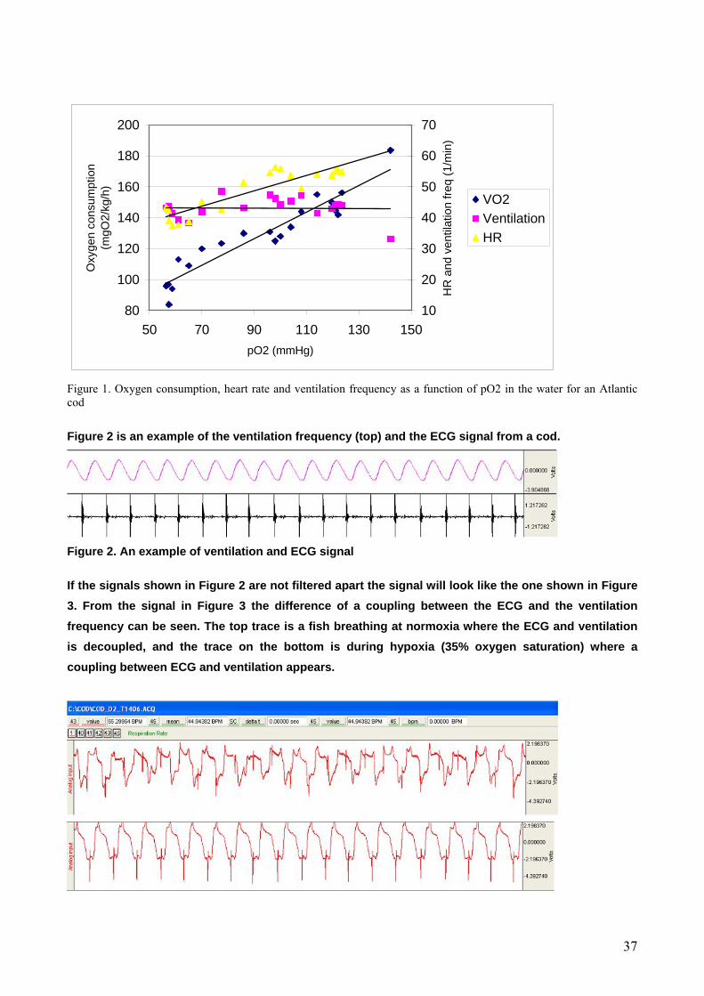
Figure 1. Oxygen consumption, heart rate and ventilation frequency as a function of pO2 in the water for an Atlantic cod Figure 2 is an example of the ventilation frequency (top) and the ECG signal from a cod.
Figure 2. An example of ventilation and ECG signal If the signals shown in Figure 2 are not filtered apart the signal will look like the one shown in Figure 3. From the signal in Figure 3 the difference of a coupling between the ECG and the ventilation frequency can be seen. The top trace is a fish breathing at normoxia where the ECG and ventilation is decoupled, and the trace on the bottom is during hypoxia (35% oxygen saturation) where a coupling between ECG and ventilation appears.
37
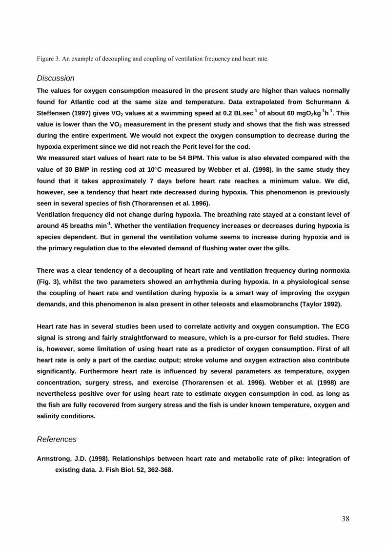
Figure 3. An example of decoupling and coupling of ventilation frequency and heart rate.
Discussion The values for oxygen consumption measured in the present study are higher than values normally found for Atlantic cod at the same size and temperature. Data extrapolated from Schurmann & Steffensen (1997) gives VO2 values at a swimming speed at 0.2 BLsec-1 of about 60 mgO2kg-1h-1. This value is lower than the VO2 measurement in the present study and shows that the fish was stressed during the entire experiment. We would not expect the oxygen consumption to decrease during the hypoxia experiment since we did not reach the Pcrit level for the cod. We measured start values of heart rate to be 54 BPM. This value is also elevated compared with the
value of 30 BMP in resting cod at 10°C measured by Webber et al. (1998). In the same study they
found that it takes approximately 7 days before heart rate reaches a minimum value. We did, however, see a tendency that heart rate decreased during hypoxia. This phenomenon is previously seen in several species of fish (Thorarensen et al. 1996). Ventilation frequency did not change during hypoxia. The breathing rate stayed at a constant level of around 45 breaths min-1. Whether the ventilation frequency increases or decreases during hypoxia is species dependent. But in general the ventilation volume seems to increase during hypoxia and is the primary regulation due to the elevated demand of flushing water over the gills. There was a clear tendency of a decoupling of heart rate and ventilation frequency during normoxia (Fig. 3), whilst the two parameters showed an arrhythmia during hypoxia. In a physiological sense the coupling of heart rate and ventilation during hypoxia is a smart way of improving the oxygen demands, and this phenomenon is also present in other teleosts and elasmobranchs (Taylor 1992). Heart rate has in several studies been used to correlate activity and oxygen consumption. The ECG signal is strong and fairly straightforward to measure, which is a pre-cursor for field studies. There is, however, some limitation of using heart rate as a predictor of oxygen consumption. First of all heart rate is only a part of the cardiac output; stroke volume and oxygen extraction also contribute significantly. Furthermore heart rate is influenced by several parameters as temperature, oxygen concentration, surgery stress, and exercise (Thorarensen et al. 1996). Webber et al. (1998) are nevertheless positive over for using heart rate to estimate oxygen consumption in cod, as long as the fish are fully recovered from surgery stress and the fish is under known temperature, oxygen and salinity conditions.
References Armstrong, J.D. (1998). Relationships between heart rate and metabolic rate of pike: integration of
existing data. J. Fish Biol. 52, 362-368.
38
Beddow T.A. and McKinley R.S. (1999). Importance of electrode positioning in biotelemetry studies estimating muscle activity in fish. J. Fish Biol. 51 (4). 819-831.
Briggs, C.T. and Post, J.R. (1997). Field metabolic rates of rainbow trout estimated using
electromyogram telemetry. J. Fish Biol. 51, 807-823. Gillis G.B. (1998). Neuromuscular control of anguilliform locomotion: patterns of red and white
muscle activity during swimming in the American eel Anguilla rostrata. J. Exp. Biol. 201, 3245-3256.
Laitinen M. and Valtonen T. (1994). Cardiovascular, ventilatory and total activity responses of brown
trout to handling stress. J. Fish Biol. 45, 933-942. McKenzie D.J., Taylor, E.W., Bronzi P. and Bolis C.L. (1995). Aspects of cardioventilatory control in
the Adriatic sturgeon (Acipenser naccarii). Resp. Physiol. 100, 45-53. Randall D.J. (1970). The circulatory system. In: Fish Physiology (Eds. Hoar W.S. and Randall D.J.)
Volume IV. pp 133-172. Schurmann H. and Steffensen J.F. (1997). Effects of temperature, hypoxia and activity on the
metabolism of Atlantic cod, Gadus morhua. J. Fish Biol. 50, 1166-1180. Steffensen J. F., Lomholt J. P. and Johansen. K. (l982). Gill ventilation and O2 extraction during
graded hypoxia in two ecologically distinct species of flatfish, the flounder, Platichthys flesus, and the plaice Pleuronectes platessa. Env. Biol. Fish. 7; 157-163.
Taylor E.W. (1992). Nervous control of the heart and cardiorespiratory interactions. In: Fish
Physiology (Eds. Hoar, W.S, Randall, D.J. and Farrell, A.P.). Vol XII, part B. pp. 343-387.
Thorarensen H., Gallaugher P.E. and Farrell A.P. (1996). The limitations of heart rate as a predictor of
metabolic rate in fish. J. Fish Biol. 49, 226-236. Webber D.M., Boutilier R.G. and Kerr S.R. (1998). Cardiac output as a predictor of metabolic rate in
cod (Gadus morhua). J. Exp. Biol. 201, 2779-2789. Økland, F., Finstad, B., McKinley, R.S., Thorstad, E.B. and Booth, R.K. (1997). Radio transmitted
electromyogram signals as indicators of physical activity in Atlantic salmon. J. Fish Biol. 51, 476-488.
39

Energy budget of North Sea whiting (Merlangius merlangus L.)
Report for a Ph.D. course held at Marine Biology Laboratory, Helsingør, 2003
Mikkel K. Sand & Anders D. Jordan
ABSTRACT A complete energy budget model was established and parameterized for North Sea whiting by combining field data on stomach contents, a gastric evacuation model and a static energy budget (SEB) model. Four scenarios are presented, each containing an expression of differently modulated net food conversion efficiencies. We found that an activity, growth and energy density modulated model was best at describing the energy expenditures allocated to swimming activity. This conclusion is partly based on concurrence between the model results and the cost of activity at optimal swimming speed for whiting.
INTRODUCTION
Fisheries management is bassed on modellers ability to develop and parameterize models estimating e.g. population growth and consumption. For this purpose primarily two kinds of models have been used – static energy budget models and gastric evacuation models. In the present study we combine two such models in order to estimate of the cost of swimming activity of whiting in the wild. A gastric evacuation model: Andersen (2001) reported a square root model to describe the evacuation of stomach content of individual piscivorous teleosts:
0.5/ SdtdS c ρ−= (1) C is the total energy content of consumed prey, ρ is the gastric evacuation rate constant, and S is the mass of the stomach content. Over a longer period of time the change in stomach content is negligible compared to the total amount of consumed prey during that period, and the change in stomach content can be set to zero, and equation 1 can be rewritten as:
0.5SC ρ= (2) By collecting and analysing a representative population subset of stomachs for amount and composition of prey, overall population consumption can be estimated using the laboratory derived gastric evacuation model. Knowing the energy densities of the different prey groups and sizes, combined with the size of predators and ambient temperature, total consumed energy can be estimated. Static energy budget model: The static energy budget model is an equation with available net energy on one side, and the different “costs of being” one the other. Presented below is the a static energy budget model:
κC = PB + PG + RS + RA (3)
40

Where, κ is the net food conversion efficiency, which, when multiplied with C (= the food consumption) describes available net energy left from a meal after the energy in faeces, exogenous excretion and SDA has been withdrawn. PB and PG is the somatic and gonad growth and RS and RA the expenses due to standard metabolic rate and activity. Combining the SEB and the gastric evacuation model it is possible to solve for the activity metabolism. With all other model components estimated, swimming activity can be quantified. The aim of the present study was to parameterise a SEB model, facilitating predictions of overall performance of whiting in the North Sea.
MATERIALS & METHODS Food consumption rate for whiting (C kj d-1) was expressed as maximum feeding rate multiplied by the actual feeding level ƒ. Maximum feeding rate, as a function of fish length and ambient temperature was parameterised [equation 4] by Andersen & Riis-Vestergaard (2003).
Cmax = 0.00737 L 2.28 e 0.0765T (4)
Where L is total fish length in cm, and T is ambient temperature ( ºC). As laboratory fish often are fatter than their relatives in the wild, fish length is applied as effector variable in equation 4, rather than mass. Overall ƒ-values was calculated by accumulating values of food consumption of all 4 quarters year, divided by the accumulated corresponding maximum food intake. Net conversion efficiency A net food conversion efficiency (κ ) for whiting fed on natural prey was estimated by Andersen & Riis-Verstergaard (2003) to be described by a simple power function.
κ lab = 0.426C0.109 (4) The lipid-protein ratio (re) for whiting can be estimated using equation (5)
κlab = 0.977(2.78-re)-0,8745 (5)
Solving equation (5) for re, the lipid – protein energy ratio of incorporated somatic biomass as a function of consumption is given by equation (6).
re = 2.78-2.74C-0.129 (6) Fishes in wild have increased level of activity as compared to laboratory fish used for establishment of equation 1-4, and consequently a minor lipid fraction is incorporated. In order to estimate the net conversion efficiency for whiting in the wild (κ wild ) an estimate of this extra cost is needed. This fraction can be expressed as:
RA* = RA – (RR(10) –RS(10)) (7) ’
Where RA* is that extra cost of activity of wild fish, RA being the activity cost of wild fish. RR(10) is the routine metabolism (maintenance costs including activity) and RS(10), the standard metabolism, both at 10 degrees celcius. The extra activity cost is reflected in the lipid protein ratio, thus an altered re is calculated in respect to κ wild [equation 7].
κ wild = 0.997[2.78-(PB, lip – RA*)(P+B,pro + RA*)-1 ] –0.8745 (8)
41

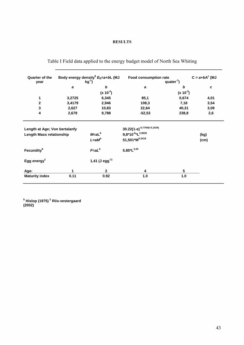
Consequently as the lipid ratio decreases as a result of extra cost of activity, the net conversion efficiency drops. Values for κwild is given in table II. Standard and routine metabolism Standard metabolic rate for whiting was expressed using a general relationship for gadoids, where RS = 5.52M0.75·e0.08T KJ d-1, where M is mass, and T is temperature in Celsius (º C). Maximum food intake as a function of length was determined from growth trials with whiting fed ad libitum at 9.7 º C in the laboratory. Relationship between routine metabolism (maintenance and activity) and mass for whiting was established from growth trials at 9.7 °C, and found to be 14.4M0.81 (Andersen & Riis-vestergaard, 2003). Routine metabolism was estimated from a laboratory experiment where whiting of a certain size was given different meal sizes – different consumption rates. Growth expressed as energy increment (kJ day-1) was calculated as function of consumption (kJ day-1). Routine metabolism was found by extrapolating this relationship to a value of zero. FIELD DATA Food consumption rates were obtained from data sets from the international stomach sampling project in 1991, preformed by ICES (Hislop, 1997). Stomach content of whiting distributed in the North Sea sampled over 4 quarters, where analysed in order to estimate total consumption. Data from year class 6+ was not used to estimate the parameters used in the model, as it consists of all age groups from 6 years and above. Futhermore we parameterised the von Bertalanffy equation using length and age from the above mentioned ICES survey. Somtatic growth and egg production Energy content of whiting eggs was calculated using a general observed value of 1.41 J egg –1 for Atlantic cod (Riis-Vestergaard, 2002), assuming no difference exists between closely related gadoids. Fecundity of whiting inhabiting the North Sea, was expressed by F = 5.85LT 3,25 (Hislop & Hall, 1974). Index of maturity was given by Andersen (pers. comm.), and is presented in table II. From these data total gonad growth (kJ day-1) was estimated, assuming no differences between sexes. Onset of gonad growth was set to first of January each year, with a subsequent spawning 133 days later.
42
RESULTS
Table I Field data applied to the energy budget model of North Sea Whiting
Quarter of the
year Body energy density$ EB=a+bL (MJ
kg-1) Food consumption rate C = a+bAc (MJ
quater-1) a b a b c (x 10-2) (x 10-3) 1 3,2725 6,345 85,1 0,674 4,01 2 3,4179 2,946 108,3 7,18 3,54 3 2,627 10,83 22,64 40,31 3,09 4 2,679 9,788 -52,53 238,8 2,6 Length at Age; Von bertalanfy 30.22(1-e)-0,7764(t-0,1034) Length Mass relationship M=aLb 9,8*10-6*L2,9626 (kg) L=aMb 51,501*M0,3418 (cm) Fecundity$ F=aLb 5.85*L3,25 Egg energy£ 1,41 (J egg-1) Age: 1 2 4 5 Maturity index 0.11 0.92 1.0 1.0 $ Hislop (1975) £ Riis-vestergaard (2002)
43

Body length LT (cm)
14 16 18 20 22 24 26 28 30 32
Food
ratio
n C
(kJ)
100
200
300
400
500
600
700
C = 85.1 + 0.000674 LT4.01
FIG I. Food rations for whiting in first quarter as function of body length.
Body length LT (cm)
16 18 20 22 24 26 28 30 32
Food
ratio
n C
(kJ)
200
400
600
800
1000
1200
1400
C = 108 + 0.00718 LT3.54
FIG: II. Food rations for whiting in second quarter as function of body length.
Body length LT (cm)
5 10 15 20 25 30 35
Food
ratio
n C
(kJ)
0
500
1000
1500
2000
2500
C = 22.6 + 0.0431 LT3.09
FIG: III. Food rations for whiting in third quarter as function of body length.
44

Body length LT (cm)
12 14 16 18 20 22 24 26 28 30 32
Food
ratio
n C
(kJ)
0
200
400
600
800
1000
1200
1400
1600
1800
C = -52.5 + 0.239 LT2.60
FIG. IV. Food rations for whiting in fourth quarter as function of body length.
Age A (y)
0 1 2 3 4 5 6 7 8
Bod
y le
ngth
LT
(cm
)
5
10
15
20
25
30
35
LT = 30.2(1 - e -0.776(A - 0.103) )
FIG. V. Length at age relationship (von Betalanffy).
Fig. VI (a-d). Predicted allocation of net energy in North Sea whiting into standard metabolism (■), activity expenditures (■), gonads (■) and soma (■) according to a static energy budget using (a) entirely laboratory-based or (b, c & d) activity modulated model of net conversion efficiency to estimate activity expenditures. (c) growth and energy density modulated model and (d) only growth modulated. Age classes with unbalanced energy budgets have been excluded. Figure denotation used throughout.
45
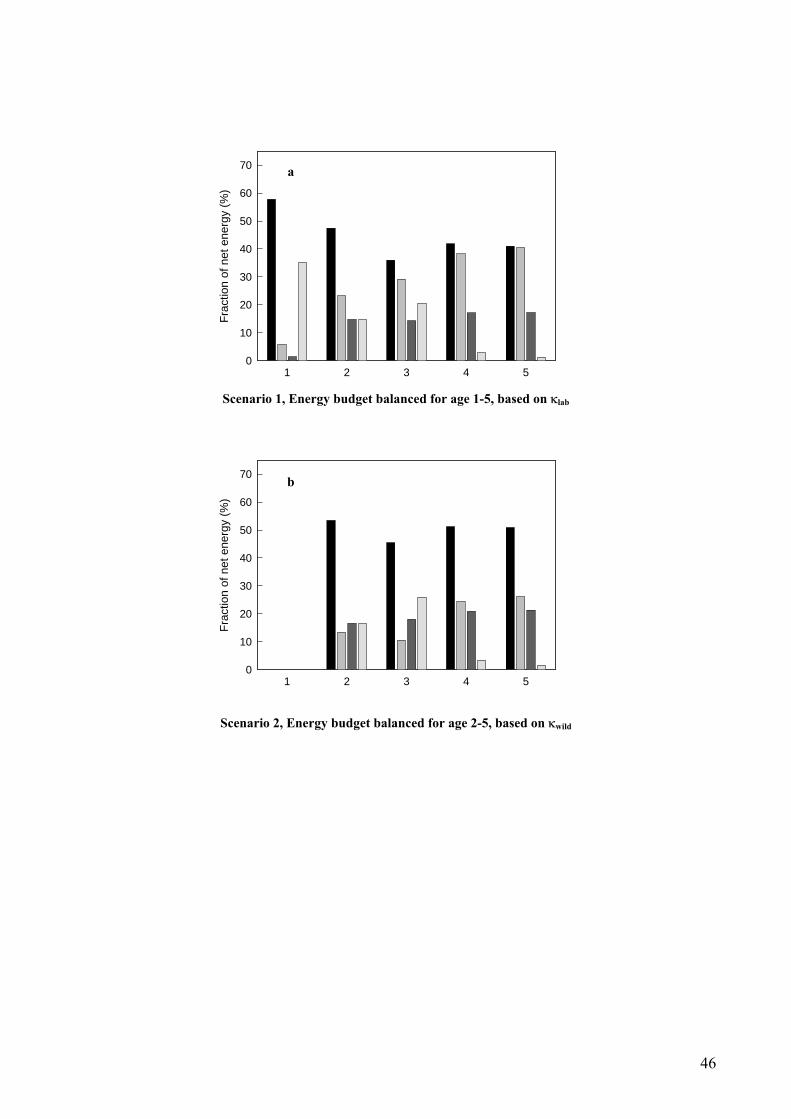
Frac
tion
of n
et e
nerg
y (%
)
0
10
20
30
40
50
60
70 a
Scenario 1
Frac
tion
of n
et e
nerg
y (%
)
0
10
20
30
40
50
60
70
Scenario 2
1 2 3 4 5
, Energy budget balanced for age 1-5, based on κlab
b
1 2 3 4 5
, Energy budget balanced for age 2-5, based on κwild
46
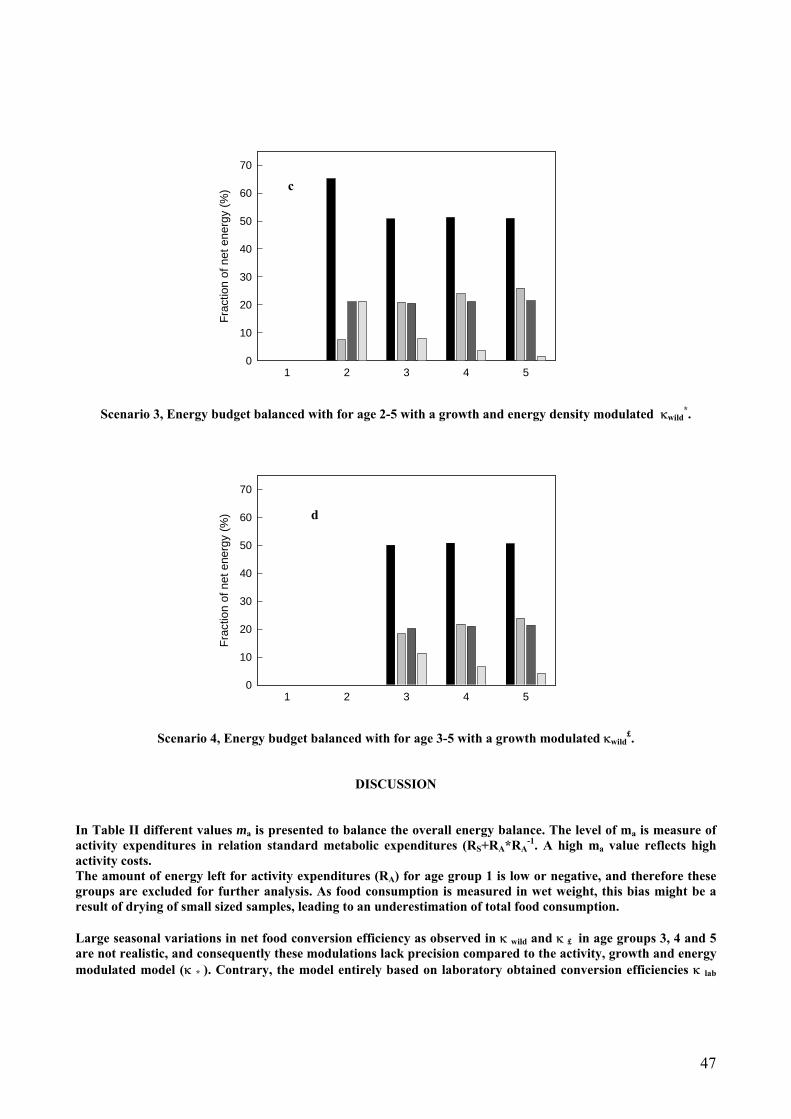
Frac
tion
of n
et e
nerg
y (%
)
0
10
20
30
40
50
60
70
c
Scenario 3, Energy budget bala
Frac
tion
of n
et e
nerg
y (%
)
0
10
20
30
40
50
60
70
Scenario 4, Energy bu
In Table II different values ma is practivity expenditures in relation staactivity costs. The amount of energy left for activgroups are excluded for further anaresult of drying of small sized sampl Large seasonal variations in net fooare not realistic, and consequently tmodulated model (κ * ). Contrary, t
1 2 3 4 5
nced with for age 2-5 with a growth and energy density modulated κwild
*.
1
d
dge
esennda
ity elysi
es, l
d cohesehe m
2 3 4 5
t balanced with for age 3-5 with a growth modulated κwild
£.
DISCUSSION
ted to balance the overall energy balance. The level of ma is measure of rd metabolic expenditures (RS+RA*RA
-1. A high ma value reflects high
xpenditures (RA) for age group 1 is low or negative, and therefore these s. As food consumption is measured in wet weight, this bias might be a eading to an underestimation of total food consumption.
nversion efficiency as observed in κ wild and κ £ in age groups 3, 4 and 5 modulations lack precision compared to the activity, growth and energy
odel entirely based on laboratory obtained conversion efficiencies κ lab
47

shows little variation, but as net conversion values rarely exceeds levels of 0.5, this modulation is imprecise. The questionable high levels of activity substantiate the latter, as a result of balancing the overall budget. Experiments on swimming metabolism for whiting has never conducted, and as a result, a precise value of optimum swimming speed (Uopt) is unknown. In the present study we chose a generalized relationship for gadoids and salmonids used by Andersen & Riis-Verstergaard (2003). Calculating the cost of swimming at Uopt for whiting (8.4 ° C), results in a level of activity of 1.35-1.56 in relation to SMR. The activity, growth and energy density model (κ *) predicts levels of activity in the range similar to Uopt in age group 3, 4 and 5 (1.37-1.47) and the model is therefore preferred. Conclusion ICES data from year first and second year class lacks of robustness to balance the energy budget. Overall we found the model (κ *) suitable to describe the allocation of net energy of north sea whiting. From figure VI, c it is seen that, the allocation of energy to SMR decreases with increasing body mass. There is a general increase in costs of activity, which seems to be energetically counteracted by a decrease in somatic growth expenditures. Gonad growth is proportionally constant after 2 years, which is a result of 92% of the population being sexually mature. However, the parameters related to the reproductive expenditures (onset gonad growth, time of spawning, energy density of eggs) are based on several assumptions, since no such data have been available. In addition seasonal length mass relations would also be desirable for improving the model.
REFERENCES Andersen, N. G. (2001) A gastric evacuation model for three predatory gadoids and implications of using pooled field data of stomach contents to estimate food rations. Journal of fish biology 59, 1198-1217 doi:10.1006/jfbi.2001.1731 Andersen, N. G., Riis-Vestergaard, J (submitted) Bioenergetics budgets og a crusing predatory fish – an evaluation of net food conversion of North Sea saithe. Journal of fish biology Hislop, J. R. G. (Ed.) (1997) Database Report of the Stomach Sampling Project 1991. ICES Cooperative Report 219. Copenhagen: International Council for the exploration of the Sea. Hislop, J. R. G. & Hall, W. B. (1974) The fecundity of whiting, Merlangius merlangus (L.) in the North Sea, the minch and at Iceland. J. cons. Int. Explor. Mer, 36:42-49 Riis-Vestergaard, J. (2002) Energy density of marine pelagic fish eggs. Journal of fish biology 60, 1511-1528. doi:10.1006/jfbi.2002.2004.
48

Evaluation of the Ph.D. Course in: Bioenergetics, biomechanics and physiology of swimming fish. Please give us your opinion on to the following questions. Do not hesitate to include supplementary comments that you find relevant. Do not write your name anywhere, it is an anonymous questionnaire. Overall evaluation What is your overall opinion about the course? Poor....................................................................................... Not very good........................................................................ OK....................................................................................…. Good...................................................................................... Excellent ............................................................................... Course content Did the course provide a reasonable overview of the subject? Yes........................................................................................ To some extent ..................................................................... No, important items were missing ....................................... Comments (e.g. missing topics) Were the topics included adequately covered? Yes........................................................................................ To some extent ..................................................................... No......................................................................................... Lectures How was the level of the lectures? Too low.................................................................................. Adequate................................................................................ Too high................................................................................. Comments Were the lectures well prepared and easy to understand? Yes........................................................................................ To some extent ..................................................................... No......................................................................................... Comments Practicals Were the exercises useful for understanding and getting hands-on experience with the subjects? Yes........................................................................................ To some extent ..................................................................... No......................................................................................... Comments
49

Course material Were the distributed papers and other material sufficient? Yes........................................................................................ To some extent ..................................................................... No......................................................................................... Comments Logistics How was the physical framework - accommodation, lecture room, food etc.? Poor....................................................................................... Not very good........................................................................ OK........................................................................................ Good...................................................................................... Excellent ............................................................................... Comments Overall balance and timing Was the balance between lectures and exercises right? Yes........................................................................................ To some extent ..................................................................... No......................................................................................... Comments Was the overall duration of the course appropriate? Too short............................................................................... Yes........................................................................................ Too long............................................................................... Comments Relevance Do you think that the course will be relevant for your career? Yes....................................................................................... Don’t know ......................................................................... Probably not ......................................................................... Not at all ............................................................................... Comments
50

Appendix A: Measuring muscle contraction times in fish This simple technique is based on a study by Wardle et al. (1989) in which twitch times of muscle in bluefin tuna were measured as a function of body size and axial position on the body. The method involves using a portable isotonic muscle transducer that provides an electrical stimulus to the muscle and records the contraction. From this record the time from stimulus to peak force can be determined. Surface strain gauges (2)
Plastic beam element
To strain gauge amplifier
To stimulator
Syringe needles
The transduce consists of a thin plastic beam onto which 4 strain guages are bonded using epoxy resin, two on the upper surface and two on the lower surface. Two syring needles are glued onto holes in the plastic beam and wired for connection to a muscle stimulator. These are inserted into the muscle, and will deflect when a contraction is initiated by the stimulator. The deflection bends the beam and this is detected by the strain gauges. These gauges are electronic resistors whose resistance varies according to the deformation (strain) imposed, and they are sensitive to very small strains. They are wired together to form an electrical circuit called a Wheatstone bridge (see below). This is a voltage divider circuit used for the measurement of static or dynamic electrical resistance. The bridge is activated by a DC voltage from the amplifier (usually 5-10V) and the output voltage of the Wheatstone bridge is expressed in millivolts output per volt input.
Strain gauge
51
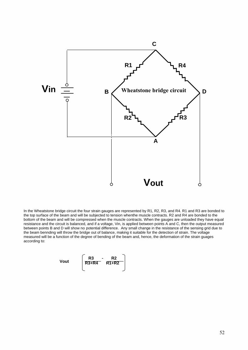
C
R4 R1
A
B
R2 R3
Vout
Wheatstone bridge circuit Vin D
In the Wheatstone bridge circuit the four strain gauges are represented by R1, R2, R3, and R4. R1 and R3 are bonded to the top surface of the beam and will be subjected to tension whenthe muscle contracts. R2 and R4 are bonded to the bottom of the beam and will be compressed when the muscle contracts. When the gauges are unloaded they have equal resistance and the circuit is balanced, and if a voltage, Vin, is applied between points A and C, then the output measured between points B and D will show no potential difference. Any small change in the resistance of the sensing grid due to the beam bennding will throw the bridge out of balance, making it suitable for the detection of strain. The voltage measured will be a function of the degree of bending of the beam and, hence, the deformation of the strain guages according to:
R3 - R2 Vout R3+R4 R1+R2
52

0 20 40 60 80 10
forc
∆t=55m
Time (ms)
0
An example of a muscle twitch experiment. Twitch time is measured from the stimulus spike to the peak force.
References:
1. Strain gauges and transducer amplifiers can be purchased from Omega Engineering (omega.com).
2. A good inexpensive stimulator can be purchased from Grass Instruments, model SD9 (http://www.grass-telefactor.com/products/stimulators/stimsd9.html). Typical stimulus pulse is 5ms duration and 2-20volts. 3. Wardle, C.S., Videler, J.J., Arimoto, T., Franco, J.M. and He, P. 1989. J. Fish Biol. 35:129-137.
53

Appendix B: Equipment used in fish course Kinematics: Swim tunnel
Digital video camera Computer for image analysis Software: Adobe Premier 6.01 video editing program
NIH Image Custom program for fish midline calculations Excel
Muscle mechanics Muscle twitch transducer Coulbourn Inc. strain gauge amplifier S72-25 Type A HP 100MHz Digital oscilloscope 5460B Software: HP 34820 Bench Link Suite data acquisition program Muscle activity (EMG) and heart rate (ECG) A-M Systems differential AC amplifier 1700
HP 100MHz Digital oscilloscope 5460B Biopac Systems MP100 data acquisition hardware
Software: AcqKnowledge data acquisition program Respirometry Swim tunnel respirometers Radiometer PHM 73 Acid Base analysers used to measure oxygen Radiometer and Loligo Oxygen electrodes Istmatec peristaltic pumps Analog video cameras. Software: Labtech Notebook, Lotus123 and Excel.
54

Course Participants: Ph-D-Student Christina Larsen Dept. of Zoophysiology University of Aarhus [email protected]: +45 89422695 e-mail: mailto:[email protected] Ph-D-Student Turid Synnøve Aas AKVAFORSK Institute of Aquaculture Research N-6600 Sunndalsøra, Norway Phone: +47 71 69 53 14 E-mail: mailto:[email protected] Ph-D-Student Johanna Lampe AKVAFORSK Institute of Aquaculture Research N-6600 Sunndalsøra, Norway Phone: +47 71 69 53 17 E-mail: [email protected] Ph-D-Student Grete Lysfjord Dept. of Fisheries and Natural Sciences Bodø Regional University N-8094 Bodø e-mail: [email protected]: +47 75 51 73 56 Pd-D-student Mikkel Sand Danmarks Fiskeriundersøgelser/Marinbiologisk Laboratorium Nordsøcentret Postboks 101 9850 Hirtshals e-mail: mailto:[email protected]: 33 96 33 00 Ph-D-Student Maria Faldborg Pedersen Marinbiologisk Laboratorium Strandpromenaden 5 3000 Helsingør e-mail: [email protected]: 49 21 33 44 Postdoc Dr. Neill A. Herbert
55

Marinbiologisk Laboratorium Strandpromenaden 5 3000 Helsingør e-mail: [email protected]: 49 21 33 44 Anders Drud Jordan Marinbiologisk Laboratorium Strandpromenaden 5 3000 Helsingør e-mail: mailto:[email protected]: 49 21 33 44 Peter Konstantinidis University of Tuebingen Spezielle Zoologie Auf der Morgenstelle 28 D- 72076 Tuebingen Germany Phone: +49 (0) 7071 2976947 e-mail: mailto:[email protected] cand. scient. Paul Maslen Marinbiologisk Laboratorium Strandpromenaden 5 3000 Helsingør e-mail: [email protected]: 49 21 33 44 Dr. Robert E. Shadwick Scripps Institution of Oceanography Marine Biology Res. Div. University of California La Jolla California 92093-0202 e-mail: [email protected]: http://sio.ucsd.edu/phone: 858-534-7973 Niels Gerner Andersen Danmarks Fiskeriundersøgelser/Marinbiologisk Laboratorium Nordsøcentret Postboks 101 9850 Hirtshals e-mail: [email protected]: http://www.dfu.min.dk/ Phone: 33 96 33 00 John Fleng Steffensen
56

Marinbiologisk Laboratorium Strandpromenaden 5 3000 Helsingør e-mail: [email protected]: http://www.mbl.ku.dk/Phone: 49 21 33 44
Other addresses: Fishnet: http://www.fishnet.dk
57
Related Documents