Slides for Chapter 3: Theory of Current Account Determination International Macroeconomics Schmitt-Groh´ e Uribe Woodford Columbia University May 1, 2016 1

Welcome message from author
This document is posted to help you gain knowledge. Please leave a comment to let me know what you think about it! Share it to your friends and learn new things together.
Transcript

Slides for Chapter 3:
Theory of Current Account Determination
International Macroeconomics
Schmitt-Grohe Uribe Woodford
Columbia University
May 1, 2016
1

International Macroeconomics, Chapter 3 Schmitt-Grohe, Uribe, Woodford
Motivation
• Build a model of an open economy to study the determinants of
the trade balance and the current account.
• Study the response of the trade balance and the current account
to a variety of economic shocks
– Changes in income
– Changes in the world interest rate
– Changes in commodity prices (e.g., oil, grain).
• Pay special attention to how those responses depend on whether
the shocks are perceived to be temporary or permanent.
2

International Macroeconomics, Chapter 3 Schmitt-Grohe, Uribe, Woodford
A Small Open Economy
What does ‘small’ and ‘open’ mean in this context?
• An economy is small when world prices and interest rates are
independent of domestic economic conditions.
• An economy is open when it trades in goods and financial assets
with the rest of the world.
• Most countries in the world are small open economies:
– Examples of developed small open economies: the Netherlands,
Switzerland, Austria, New Zealand, Australia, Canada, Norway.
– Examples of emerging small open economies: Chile, Peru, Bolivia,
Greece, Portugal, Estonia, Latvia, Thailand.
– Examples of large open economies: United States, Japan, Germany,
and the United Kingdom.
– Examples of large emerging economies: China, India
–Examples of closed economies: Perhaps the most notable cases are
North Korea, Venezuela, and to a lesser extent Cuba and Iran.
• Economic and geographic size not necessarily related: Australia
and Canada vs. UK and Japan.
3

International Macroeconomics, Chapter 3 Schmitt-Grohe, Uribe, Woodford
The Model Economy
• A two-period small open economy: periods 1 and 2.
• Households receive endowments Q1 and Q2 in periods 1 and 2,
respectively.
• Initial wealth (1 + r0)B∗0 inherited from the past. Here, B∗
0 are
bonds that paid the interest rate r0.
• In period 1, households choose consumption, C1, and bond holdings,
B∗1, which pay the interest rate r1.
4
International Macroeconomics, Chapter 3 Schmitt-Grohe, Uribe, Woodford
Sequential Budget Constraints
The period-1 budget constraint
C1 + B∗1 − B∗
0 = r0B∗0 + Q1. (1)
The period-2 budget constraint
C2 + B∗2 − B∗
1 = r1B∗1 + Q2, (2)
Because the world ends after period 2, no one is going to be around
to pay or collect debts. So bond holdings must be nil at the end of
period 2, that is,
B∗2 = 0. (3)
This expression is known as the transversality condition.
5

International Macroeconomics, Chapter 3 Schmitt-Grohe, Uribe, Woodford
The Intertemporal Budget Constraint
Combine (1), (2), and (3) to eliminate B∗1 and B∗
2. This yields
C1 +C2
1 + r1= (1 + r0)B
∗0 + Q1 +
Q2
1 + r1. (4)
This is the intertemporal budget constraint. It says that the present
discounted value of the endowment plus the initial financial wealth
(the right-had side) must be enough to pay for the present discounted
value of consumption. (the left-hand side).
The following figure provides a graphical representation of the the
intertemporal budget constraint.
6
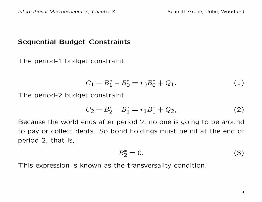
International Macroeconomics, Chapter 3 Schmitt-Grohe, Uribe, Woodford
The intertemporal budget constraint
Q1+Q
2/(1+r
1)
(1+r1)Q
1+Q
2
C1
C2
slope = − (1+r1)
A
Q1
Q2
7
International Macroeconomics, Chapter 3 Schmitt-Grohe, Uribe, Woodford
Observations On The Intertemporal Budget Constraint
• It’s slope is −(1+r1), because if you sacrifice one unit of consumption
and put it in the bank for one period, you get 1+r1 units next period.
• The set of feasible consumption baskets are those inside or at the
borders of the triangle formed by the vertical line, the horizontal
line, and the intertemporal budget constraint.
• Points outside that triangle are infeasible.
• What feasible point will the household choose depends on its
preferences. We turn to this issue next.
8

International Macroeconomics, Chapter 3 Schmitt-Grohe, Uribe, Woodford
The Lifetime Utility Function
We assume that the household happiness increases with consuming
goods in periods 1 and 2. We assume that the lifetime utility
function is of the form
lnC1 + lnC2,
where ln denotes the natural logarithm. Other specifiaitons are
possible.
Indifference Curves
An indifference curve is the set of consumption baskets (C1, C2) that
delivers the same level of welfare.
The following figure displays examples of indifference curves.
9

International Macroeconomics, Chapter 3 Schmitt-Grohe, Uribe, Woodford
Indifference Curves
C1
C2
10

International Macroeconomics, Chapter 3 Schmitt-Grohe, Uribe, Woodford
Properties of Indifference Curves
• If C1 and C2 are goods (i.e., objects for which more is preferred
to less), indifference curves are downward sloping.
• An indifference curve located northeast of another one yields higher
utility.
• Through each point crosses one indifference curve; they densely
populate the positive quadrant.
• Indifference curves do not cross one another. • Indifference curves
we focus on are convex. If you are consuming a lot in period 1
and almost nothing in period 2, you are not willing to give up much
period-2 consumption for an additional unit of consumption in period
1. But if you are consuming a almost nothing in period 1 and a lot
in period 2, you are willing to give up much period-2 consumption
for an additional unit of consumption in period 1. This is known as
diminishing marginal rate of substitution of C2 for C1.
11
International Macroeconomics, Chapter 3 Schmitt-Grohe, Uribe, Woodford
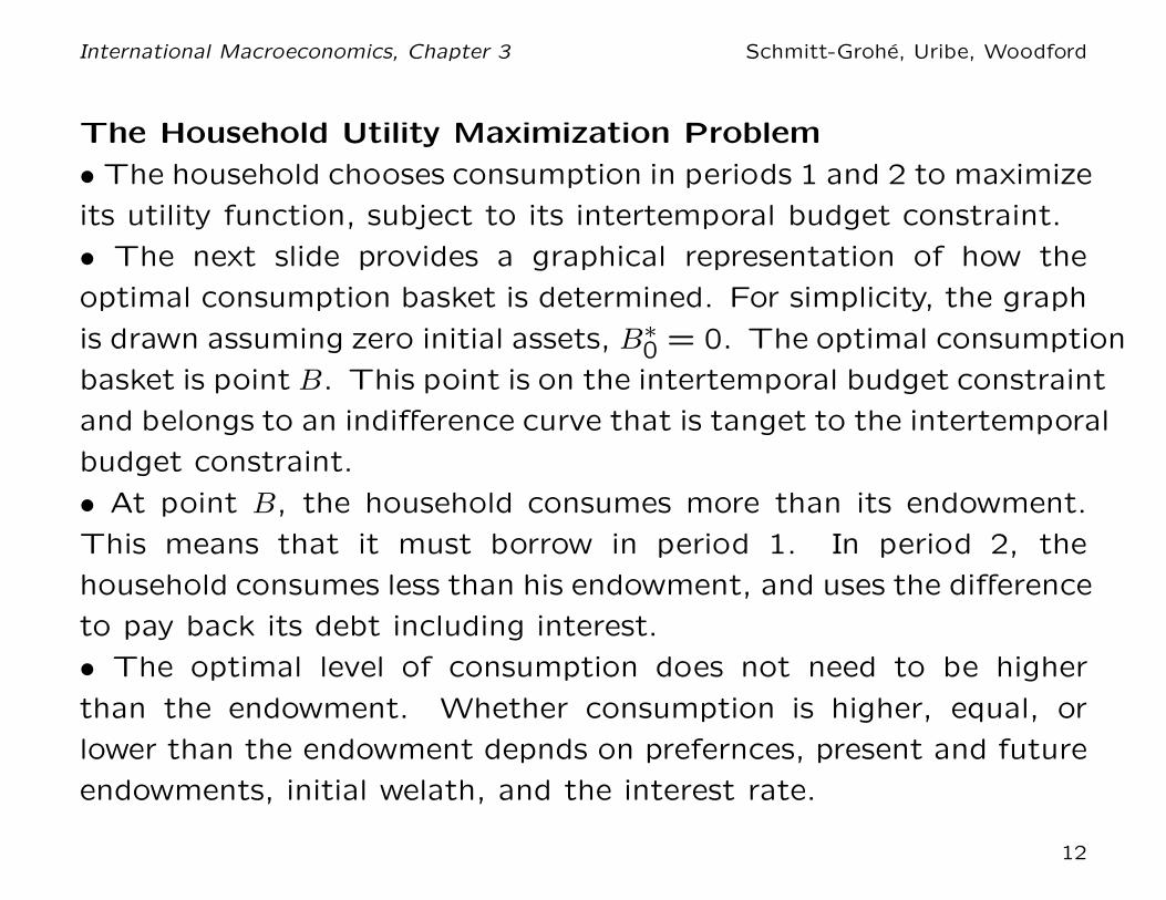
The Household Utility Maximization Problem
• The household chooses consumption in periods 1 and 2 to maximize
its utility function, subject to its intertemporal budget constraint.
• The next slide provides a graphical representation of how the
optimal consumption basket is determined. For simplicity, the graph
is drawn assuming zero initial assets, B∗0 = 0. The optimal consumption
basket is point B. This point is on the intertemporal budget constraint
and belongs to an indifference curve that is tanget to the intertemporal
budget constraint.
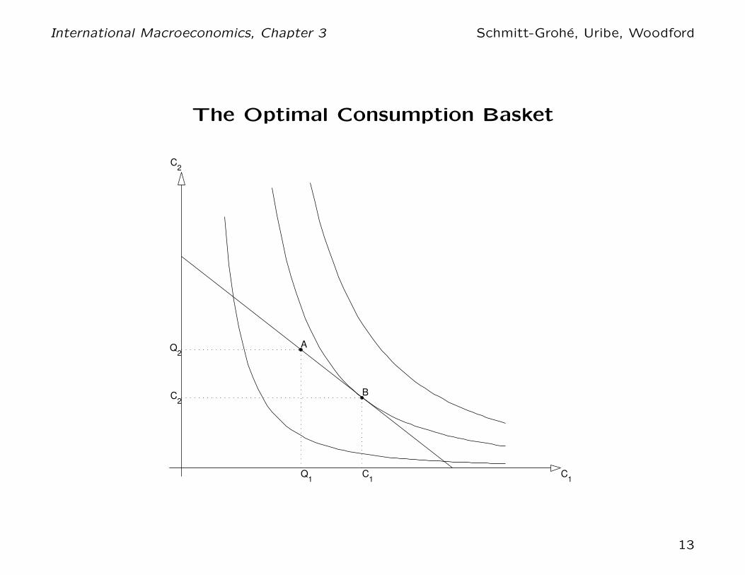
• At point B, the household consumes more than its endowment.
This means that it must borrow in period 1. In period 2, the
household consumes less than his endowment, and uses the difference
to pay back its debt including interest.
• The optimal level of consumption does not need to be higher
than the endowment. Whether consumption is higher, equal, or
lower than the endowment depnds on prefernces, present and future
endowments, initial welath, and the interest rate.
12
International Macroeconomics, Chapter 3 Schmitt-Grohe, Uribe, Woodford
The Optimal Consumption Basket
C1
C2
A
Q1
Q2
B
C1
C2
13
International Macroeconomics, Chapter 3 Schmitt-Grohe, Uribe, Woodford
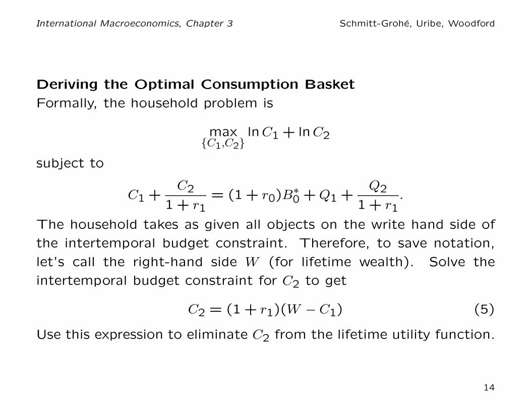
Deriving the Optimal Consumption Basket
Formally, the household problem is
max{C1,C2}
lnC1 + lnC2
subject to
C1 +C2
1 + r1= (1 + r0)B
∗0 + Q1 +
Q2
1 + r1.
The household takes as given all objects on the write hand side of
the intertemporal budget constraint. Therefore, to save notation,
let’s call the right-hand side W (for lifetime wealth). Solve the
intertemporal budget constraint for C2 to get
C2 = (1 + r1)(W − C1) (5)
Use this expression to eliminate C2 from the lifetime utility function.
14

International Macroeconomics, Chapter 3 Schmitt-Grohe, Uribe, Woodford
Deriving the Optimal Consumption Basket (Continued)
The household maximization problem then becomes
max{C1}
lnC1 + ln[(1 + r1)(W − C1)]
To maximize this expression, take the derivative with respect to C1,
equate to zero, and solve for C1. This yields
C1 =1
2W. (6)
Intuitively, the household consumes half of its lifetime wealth.Combining
(5) and (6) yields
C2 =1
2W (1 + r1). (7)
This is also intuitive. The household consumes half of W in period
1 and puts the other half in the bank, receiving 12W (1 + r1) for
consumption in period 2.
15

International Macroeconomics, Chapter 3 Schmitt-Grohe, Uribe, Woodford
Deriving the Optimal Consumption Basket (Continued)
Now recall that W = (1 + r0)B∗0 + Q1 + Q2
1+r1to write (6), as
C1 = 12
[
(1 + r0)B∗0 + Q1 + Q2
1+r1
]
According to this expression, consumption is increasing in Q1 , Q2,
and (1 + r0)B∗0, and decreasing in the interest rate r1.
It is clear from the that the response of consumption to an increase
in current output depends crucially on what households expect to
happen with future consumption. If the increase in Q1 is temporary,
so that Q2 is not expected to change, then consumption increase
by 1/2 the change in output. Households the other leave half for
future consumption. But if the increase in Q1 is expected to be
associated with an equal increase in Q2, household consume most
of the output increase (a fraction (1 + r1/2)/(1 + r1)). In this case
there is no need to leave much for tomorrow, because output will
also be high next period.
We do not observe Q2 in period 1, so the reaction of C1 allows us
to infer whether the change in Q1 is temporary or permanent.
16

International Macroeconomics, Chapter 3 Schmitt-Grohe, Uribe, Woodford
The Trade Balance and the Current Account
We can now answer the question posed at the beginning: What
determines the trade balance and the current account? The trade
balance is the difference between output and consumption, TB1 =
Q1 − C1. If desired consumption is less than output, the economy
exports goods to the rest of the world. If output falls short of desired
consumption, the economy imports goods from the rest of the world
Replacing C1 by its optimal value, we obtain
TB1 = 12
[
−(1 + r0)B∗0 + Q1 − Q2
1+r1
]
The current account equals the trade balance plus investment income,
given by r0B∗0. Thus,
CA1 = 12
[
−(1 − r0)B∗0 + Q1 − Q2
1+r1
]
17

International Macroeconomics, Chapter 3 Schmitt-Grohe, Uribe, Woodford
Free Capital Mobility and the Determination of the Interest
Rate
We assume that there is free international capital mobility. That
is, households can borrow and lend in the international financial
market. Let r∗ be the world interest rate. Then, free capital mobility
guarantees that the domestic interest rate be equal to the world
interest rate. That is,
r1 = r∗
Any difference between r1 and r∗ to give rise to an arbitrage opportunity
that would allow someone to make infinite profits. For instance
if r1 > r∗, then one could make infinite amounts of profits by
borrowing in the international market and lending in the domestic
market. Similarly, if r1 < r∗, unbounded profits could be obtained
by borrowing domestically and lending abroad. These opportunities
disappear when r1 = r∗.
18
International Macroeconomics, Chapter 3 Schmitt-Grohe, Uribe, Woodford
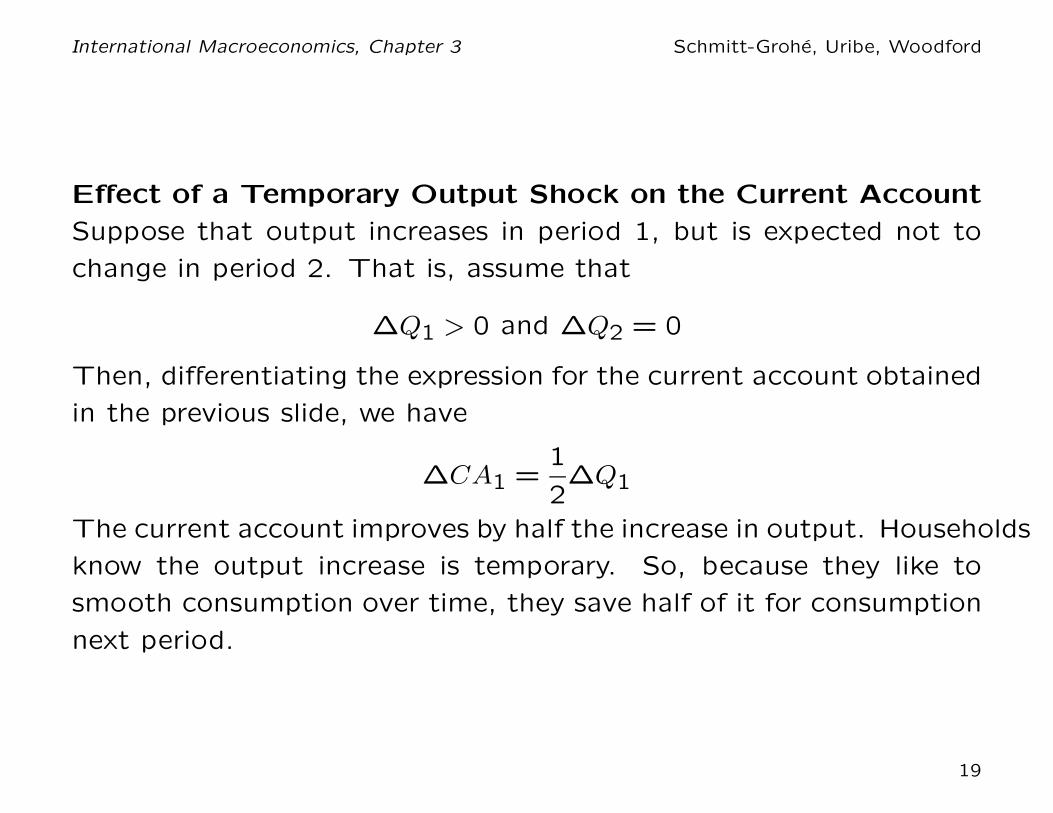
Effect of a Temporary Output Shock on the Current Account
Suppose that output increases in period 1, but is expected not to
change in period 2. That is, assume that
∆Q1 > 0 and ∆Q2 = 0
Then, differentiating the expression for the current account obtained
in the previous slide, we have
∆CA1 =1
2∆Q1
The current account improves by half the increase in output. Households
know the output increase is temporary. So, because they like to
smooth consumption over time, they save half of it for consumption
next period.
19
International Macroeconomics, Chapter 3 Schmitt-Grohe, Uribe, Woodford
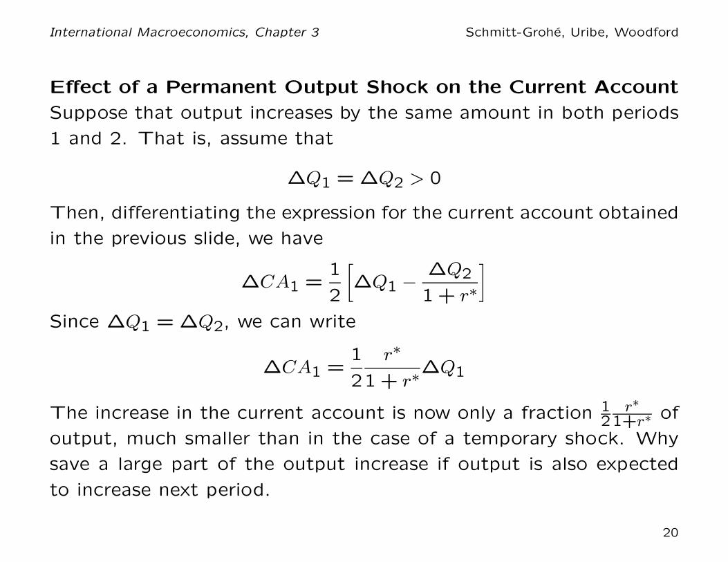
Effect of a Permanent Output Shock on the Current Account
Suppose that output increases by the same amount in both periods
1 and 2. That is, assume that
∆Q1 = ∆Q2 > 0
Then, differentiating the expression for the current account obtained
in the previous slide, we have
∆CA1 =1
2
[
∆Q1 −∆Q2
1 + r∗
]
Since ∆Q1 = ∆Q2, we can write
∆CA1 =1
2
r∗
1 + r∗∆Q1
The increase in the current account is now only a fraction 12
r∗
1+r∗ of
output, much smaller than in the case of a temporary shock. Why
save a large part of the output increase if output is also expected
to increase next period.
20
International Macroeconomics, Chapter 3 Schmitt-Grohe, Uribe, Woodford
A General Principle
If you lose your lunch money one day, it’s not a problem. You simply
borrow from a friend. Next time, you pay his lunch. However, if you
father cuts your monthly allowance, you will have to make plans
to reduce your spending accordingly. We have seen that a similar
principle is at work with the current account. We summarize this
principle as follows:
Finance temporary output shocks (by running current account
deficits or surpluses without much change in spending) and
adjust to permanent output shocks (by changing spending,
without much change in the current account).
21

International Macroeconomics, Chapter 3 Schmitt-Grohe, Uribe, Woodford
Terms-of-Trade Shocks
Thus, far we have assumed that there is just one good that can
be consumed, imported, or exported. In reality, the final goods a
country imports are different from the goods it exports. Consider,
for instance, an oil producing country that exports oil and oil derivatives
and imports consumption goods, such as food, textiles, electronics,
etc.
Changes in the relative price of exports can have macroeconomic
effects on consumption, the trade balance, and the current account.
We will show that these effects are very similar to endowment
shocks.
The relative price of exportable goods in terms of importable goods
is known as the terms of trade. Letting PX denote the price of
exportables and PM the price of importables, the terms of trade,
which we denote by TT , are given by
TT =PX
PM
22
International Macroeconomics, Chapter 3 Schmitt-Grohe, Uribe, Woodford
Importable Goods, Exportable Goods, and the Terms of Trade
Suppose that the endowment Q1 is a good that households do not
consume, say oil. However, households can export this good at the
world price PX1 . The country does not produce consumption goods,
say food, but can import them at the world price PM1 . Before,
bonds were denominated in the single consumption good. Now,
assume that bonds are denominated in units of importable goods.
The budget constraint of the household in period 1 is then given by
PM1 C1 + PM
1 B∗1 − PM
1 B∗0 = PM
1 r0B∗0 + PX
1 Q1.
Dividing both sides by PM1 , we obtain
C1 + B∗1 − B∗
0 = r0B∗0 + TT1Q1. (8)
Similarly, in period 2, the budget constraint of the household is
C2 + B∗2 − B∗
1 = r1B∗1 + TT2Q2. (9)
23

International Macroeconomics, Chapter 3 Schmitt-Grohe, Uribe, Woodford
Terms-of-Trade Shocks Are Just Like Endowment Shocks
Combining (8) with (9) and the transversality condition (3), we
obtain the the intertemporal budget constraint
C1 +C2
1 + r1= (1 + r0)B
∗0 + TT1Q1 +
TT2Q2
1 + r1. (10)
This expression is identical to its counterpart in the one-good model
(see equation (4)), except that the endowments Q1 and Q2 in the
one-good model are replaced by TT1Q1 anbd TT2Q2. By multiplying
Q1 by TT1, we are expression the endowment of exportable goods
(oil) in terms of importable goods (food), so that in the budget
constraint all terms are measured in the same units.
The present economy is small, so it takes TT1 and TT2 as given,
just as it takes as given Q1 and Q2. It follows that changes in the
terms of trade are just like changes in the endowment.
24

International Macroeconomics, Chapter 3 Schmitt-Grohe, Uribe, Woodford
Effect of Term-of-Trade Shocks on the Current Account
We have shown that terms-of-trade shocks are just like endowment
shocks. It follows that the effect of a terms-of-trade shocks on the
trade balance and the current account depend crucially on whether
the terms-of-trade shock is perceived as temporary or permanent.
Temporary changes in the terms of trade will tend to have large
effects on the trade balance and the current account and permanent
terms-of-trade shocks will tend to have a small effect.
Finance temporary terms-of-trade shocks shocks (by running
current account deficits or surpluses without much change
in spending) and adjust to permanent terms-of-trade shocks
shocks (by changing spending, without much change in the
current account).
We now test how this principle works in real life.
25

International Macroeconomics, Chapter 3 Schmitt-Grohe, Uribe, Woodford
Temporary versus Permanent Terms of Trade Shocks
A Case Study of the Copper Price in Chile 2001-2013
Take a look at the next slide, which shows the real price of copper
between 2001 and 2013.
Copper accounts for more than 50 percent of Chilean exports. Thus,
variations in world copper prices represent important terms of trade
shocks for Chile.
26

International Macroeconomics, Chapter 3 Schmitt-Grohe, Uribe, Woodford
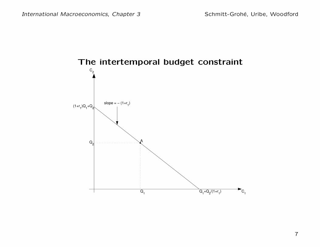
Real Price of Copper, Chile, 2001Q1-2013Q4
2001 2003 2005 2007 2009 2011 20130
100
200
300
400
500
600
Ind
ex (
20
03
=1
00
)
Data Source: Fornero and Kirchner, 2014.
27

International Macroeconomics, Chapter 3 Schmitt-Grohe, Uribe, Woodford
Observations on the figure.
The copper price starts increasing in 2003 and stays high until 2013
(except for a short dip in 2009, during the Great Recession).
Look at the units on the vertical axis. Between 2003 and 2007 the
real price of copper increases by almost 400 percent! This is an
enormous price increase.
And this price increase was of the permanent variety, in the sense
that the copper price stayed that high from 2006 to 2013.
What does our theory of current account determination say, should
have happened to the CA between 2003 and 2007 in response to
the copper price increase?
Recall the principle, “finance temporary shocks and adjust to permanent
ones.” Our theory thus predicts that the current account should be
little changed.
28

Or if we assume that forward looking agents were anticipating the
gradual increase of the copper price between 2003 and 2007 they
should have initially borrowed against this permanent terms of trade
appreciation. So our model predicts either no CA change or, if
anything, a CA deterioration.
Let’s look if this prediction of our model is borne out in the data.
What happened to the CA between 2003 and 2007?
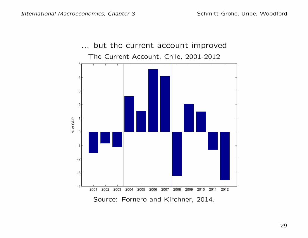
International Macroeconomics, Chapter 3 Schmitt-Grohe, Uribe, Woodford
... but the current account improved
The Current Account, Chile, 2001-2012
2001 2002 2003 2004 2005 2006 2007 2008 2009 2010 2011 2012−4
−3
−2
−1
0
1
2
3
4
5
% o
f G
DP
Source: Fornero and Kirchner, 2014.
29

International Macroeconomics, Chapter 3 Schmitt-Grohe, Uribe, Woodford
What to make of this? Is the model wrong? Or was the model right
but the change in the copper price was not the main shock hitting
the Chilean economy at that point?
Is there a way that our model would predict that the CA response to
the terms of trade appreciation is a current account appreciation?
yes, our model would predict that provided the terms of trade appreciation
was considered to be temporary. We already saw that the copper
price increase was of a permanent type. But for our model what
counts is not what is true ex post but what people were thinking
while the copper price was sky-rocketing, that is, during 2003-2007.
Look at the next figure. It shows the 10-year ahead forecast of the
price of copper, that is, the 2003 observations gives the forecast for
the year 2013, and so on. Did people think the copper price increase
was temporary or permanent.
30

International Macroeconomics, Chapter 3 Schmitt-Grohe, Uribe, Woodford
... People expected the copper price increase to be temporary!
Ten-Year Forecast and Actual Real Price of Copper, Chile, 2001-2013
2001 2003 2005 2007 2009 2011 20130
100
200
300
400
500
600In
dex (
2003=
100)
Ten−Year Ahead Forecast
Actual Copper Price
Data Source: Fornero and Kirchner, 2014.
31

International Macroeconomics, Chapter 3 Schmitt-Grohe, Uribe, Woodford
Observations on the figure.
The circled-line shows the 10-year ahead forecast of the real copper
price. This forecast remained at the 2003 level throughout the
period 2003 to 2007. In 2003 the forecasted price for 2013 was
100, that is, the same price it had in 2003, and in 2007 it was only
slightly higher, at 137. At that time the actual copper price was
at 400. So, the figure shows clearly that agents did not expect the
copper price increase to last.
That is, agent’s thought the copper price increase was temporary.
In that case, our model predicts that the current account should
appreciate, which is was indeed was observed.
32

International Macroeconomics, Chapter 3 Schmitt-Grohe, Uribe, Woodford
Effect of an Interest Rate Shock
An increase in the world interest rate, r∗, has multiple, potentially
conflicting, effects on consumption, the trade balance and the current
account.
• The Substitution Effect: An increase in the interest rate makes
savings more attractive, so households substitute present consumption
with future consumption. Thus, consumption falls and the trade
balance and the current account improve.
Substitution Effect: r∗ ↑⇒ C1 ↓, TB1 ↑, CA1 ↑
• Wealth Effect: An increase in the interest rate makes debtors
poorer and creditors richer.
Wealth Effect: r∗ ↑⇒
{
C1 ↓, TB1 ↑, CA1 ↑ if debtorC1 ↑, TB1 ↓, CA1 ↓ if creditor
Which effect dominates? We will assume that the substitution
effect always dominates. This is the case in the economy with log
preferences, as we show next.
33

International Macroeconomics, Chapter 3 Schmitt-Grohe, Uribe, Woodford
Substitution and Wealf Effects: Which Dominates?
Consider the economy with log preferences analyzed earlier. We
reproduce the equilibrium expression for consumption, the trade
balance, and the current account:
C1 =1
2
[
(1 + r0)B∗0 + Q1 +
Q2
1 + r∗
]
TB1 =1
2
[
−(1 + r0)B∗0 + Q1 −
Q2
1 + r∗
]
CA1 =1
2
[
−(1 − r0)B∗0 + Q1 −
Q2
1 + r∗
]
The first expressioin shows that consumption falls as the interest
rate increases, and the last two expressions show that both the
trade balance and the current account improve. In this economy,
the substitution effect clearly dominates the wealth effect.
The next graph illustrates what happens when r∗ goes up.
34

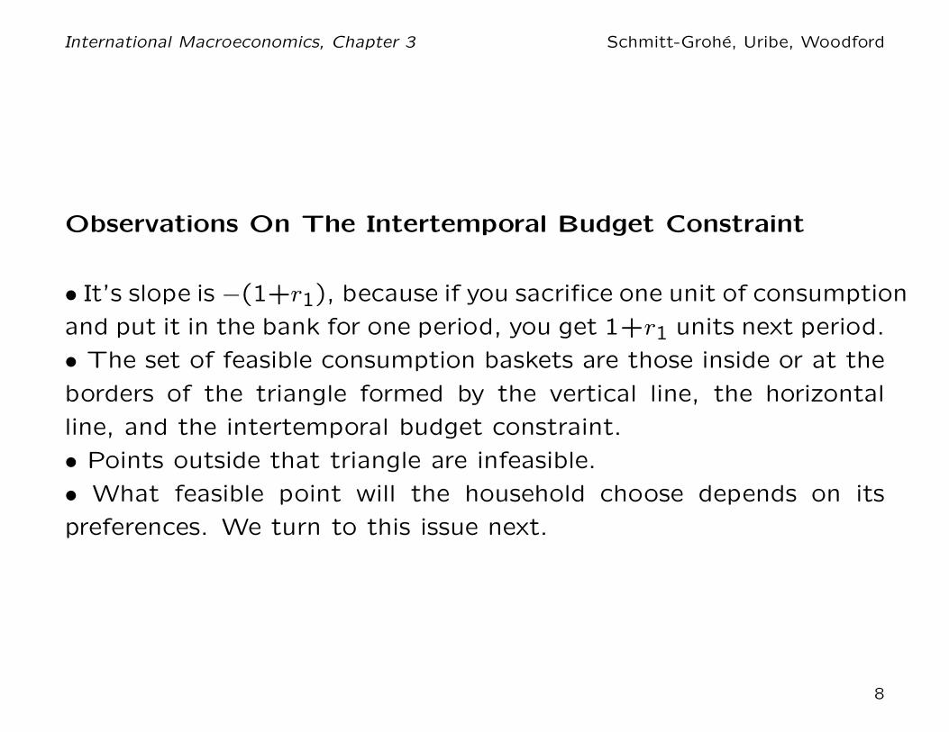
International Macroeconomics, Chapter 3 Schmitt-Grohe, Uribe, Woodford
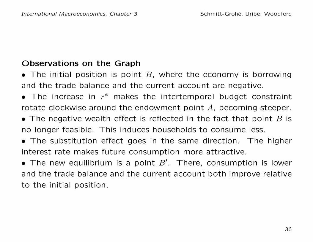
Adjustment to a World Interest Rate Shock
C1
C2
A
Q1
Q2
B
C1
C2
B′
C1
′
C2
′
← slope = − (1+r* +∆)
35
International Macroeconomics, Chapter 3 Schmitt-Grohe, Uribe, Woodford
Observations on the Graph
• The initial position is point B, where the economy is borrowing
and the trade balance and the current account are negative.
• The increase in r∗ makes the intertemporal budget constraint
rotate clockwise around the endowment point A, becoming steeper.
• The negative wealth effect is reflected in the fact that point B is
no longer feasible. This induces households to consume less.
• The substitution effect goes in the same direction. The higher
interest rate makes future consumption more attractive.
• The new equilibrium is a point B′. There, consumption is lower
and the trade balance and the current account both improve relative
to the initial position.
36

International Macroeconomics, Chapter 3 Schmitt-Grohe, Uribe, Woodford
Capital Controls
Sometimes, governments try to curb current-account deficits on the
grounds that, by causing debt to increase, are the harbinger of crises
and reduced consumption in the future.
• In their more severe form, capital controls prohibit international
borrowing.
• Milder forms include taxes on international borrowing or on interest
on external debt.
• Questions: Are capital controls effective in boosting future consumption?
Are capital controls welfare enhancing?
• Take the strong form of capital controls; a regulation requiring that
B∗1 ≥ 0
According to this regulation, it is allowed to lend to the rest of the
world, but not to borrow from the rest of the world.
37

International Macroeconomics, Chapter 3 Schmitt-Grohe, Uribe, Woodford
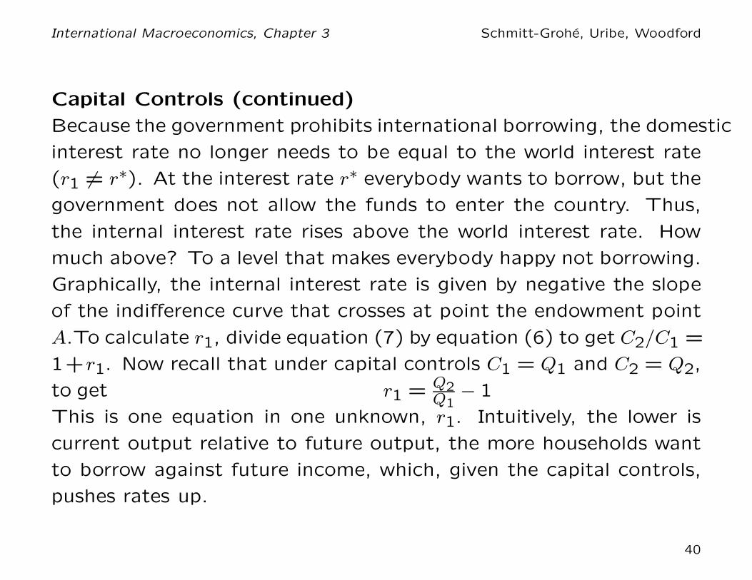
Capital Controls (continued)
The graph on the next page illustrates the situation. For simplicity,
the figure assumes no initial debt or assets (B∗0 = 0)
• The unconstrained equilibrium is at point B. This point is located
southeast of the endowment point A. This means that C1 > Q1 and
that the economy is borrowing from the rest of the world (B∗1 < 0).
• When capital controls are imposed, the welfare maximizing consumption
basket is the endowment, point A. There, borrowing is zero (B∗1 =
0).
• Answers to the questions posed above: yes, the restriction is
effective in boosting future consumption (see the figure). No, capital
control policy is not welfare enhancing. The indifference curve that
crosses A is down and to the left of the one that crosses B.
38

International Macroeconomics, Chapter 3 Schmitt-Grohe, Uribe, Woodford
Equilibrium Under Capital Controls
slope = − (1+r1) →
C1
C2
A
Q1
Q2
B
slope = − (1+r*)
39
International Macroeconomics, Chapter 3 Schmitt-Grohe, Uribe, Woodford
Capital Controls (continued)
Because the government prohibits international borrowing, the domestic
interest rate no longer needs to be equal to the world interest rate
(r1 6= r∗). At the interest rate r∗ everybody wants to borrow, but the
government does not allow the funds to enter the country. Thus,
the internal interest rate rises above the world interest rate. How
much above? To a level that makes everybody happy not borrowing.
Graphically, the internal interest rate is given by negative the slope
of the indifference curve that crosses at point the endowment point
A.To calculate r1, divide equation (7) by equation (6) to get C2/C1 =
1+r1. Now recall that under capital controls C1 = Q1 and C2 = Q2,
to get r1 = Q2Q1
− 1
This is one equation in one unknown, r1. Intuitively, the lower is
current output relative to future output, the more households want
to borrow against future income, which, given the capital controls,
pushes rates up.
40
Related Documents