lide Source: Ha Yoon Song ICT, TUWien Overview of Mobility Models

Welcome message from author
This document is posted to help you gain knowledge. Please leave a comment to let me know what you think about it! Share it to your friends and learn new things together.
Transcript
Slide Source: Ha Yoon Song
ICT, TUWien
Overview of Mobility Models
1. Introduction
• Use a mobility model in order to thoroughly simulate a new protocol
• Trace and Synthetic models plus
• Trace are those mobility patterns that are observed in real life systems.
• Synthetic models attempt to realistically represent the behaviors of MNs without the use of traces.

3
Mobility
Static (e.g., sensor networks)
MobileControlled Mobility
Uncontrolled Mobility
Hybrid
Predictable Mobility
Unpredictable Mobility
Hybrid
Hybrid
Classification of Mobility and Mobility Models
I- Based on Controllability
II- Based on Model Construction
Model
Synthetic
Trace-basedMovement Pattern
Usage pattern
Hybrid
Hybrid

4
Mobility Dimensions & Classification of Synthetic Uncontrolled Mobility Models
* F. Bai, A. Helmy, "A Survey of Mobility Modeling and Analysis in Wireles Adhoc Networks", Book Chapter in the book "Wireless Ad Hoc and Sensor Networks”, Kluwer Academic Publishers, June 2004.
2. Entity Mobility Models
• Random Walk• Random Waypoint• Random Direction• A Boundless Simulation Area• Gauss-Markov• A probabilistic Version of Random Walk
2.1 Random Walk(2.1.1 Overview)
• The Random Walk Mobility Model was first described mathematically by Einstein in 1926.
• In this mobility model, an MN moves from its current location to a new location by randomly choosing a direction and speed.
• Speed:[speedmin, speedmax], direction:[0,2π]
• A constant time interval t or a constant distance traveled d.
• There are 1-D, 2-D, 3-D and d-D walks • but 2-D Random Walk Mobility Model is of special interest.
The Random Walk Mobility Model is a widely used mobility model.
2.1 Random Walk(2.1.1 Overview)

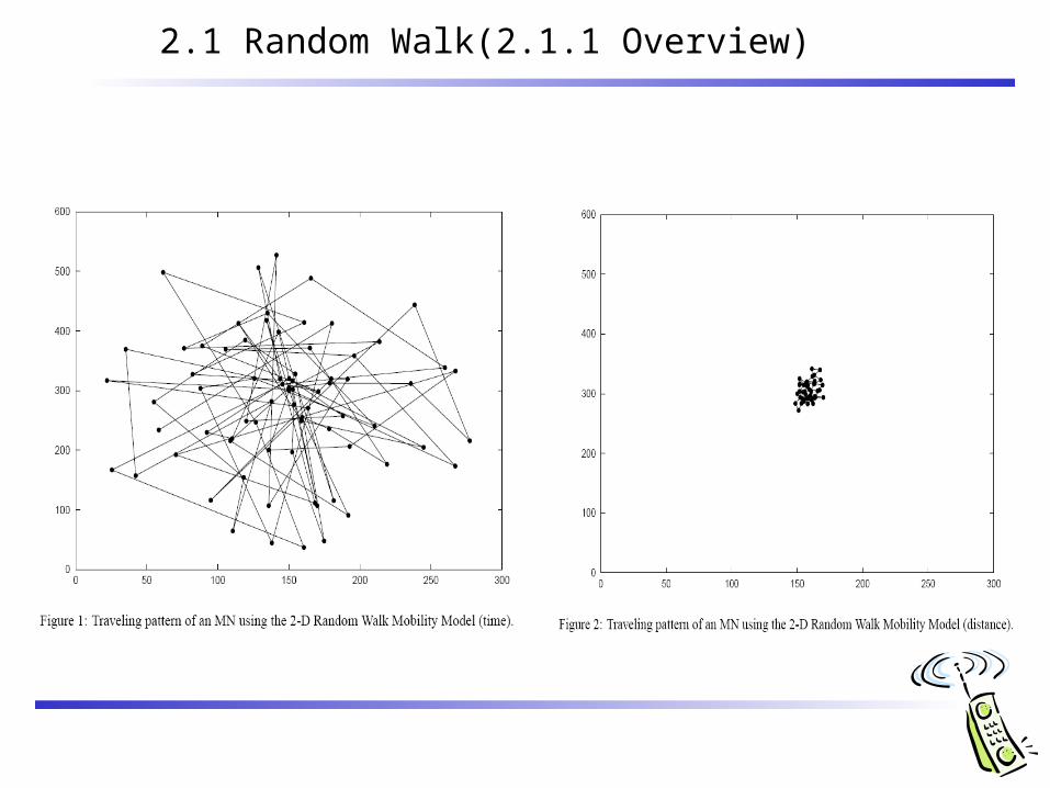
2.1 Random Walk(2.1.2 Discussion)
• The Random Walk Mobility Model is a memory-less mobility pattern.
• The current speed and direction of an MN is independent of its past speed and direction.
• This characteristic can generate unrealistic movements such as sudden stops and sharp turns.(Gauss-Markov mobility can fix this discrepancy)
• • Figure 2, the MN does not roam for from its initial position.
2.2 Random Waypoint(2.2.1 Overview)
• The Random Waypoint Mobility Model includes pause times between changes in direction and/or speed.
• An MN begins by staying in one location for a certain period of time
• Choose a random destination and speed [minspeed, maxspeed]
• Random Waypoint Mobility Model is similar to the Random Walk Mobility Model.(pause time = 0, [minspeed, maxspeed] = [speedmin, speedmax]).
• The Random Waypoint Mobility Model is also a widely used mobility model.

2.2 Random Waypoint(2.2.1 Overview)

2.2 Random Waypoint(2.2.1 Discussion)
• The MNs are initially distributed randomly around the simulation area.• A neighbor of an MN is a node within the MN’s transmission range.• The high variability in average MN neighbor percentage will produce
high variability in performance results.
Presently, three possible solutions to avoid this initialization problem. Save the locations of the MNs after a simulation has executed long. Initially distribute the MNs in a manner that maps to a distribution more
common to the model. Lastly, Discard the initial 1000 seconds of simulation time.
2.2 Random Waypoint(2.2.1 Discussion)
• A complex relationship between node speed and pause time.
• A scenario with slow MNs and long pause times actually produces a more stable network than a scenario with fast MNs and shorter pause times.
• If the Random Waypoint Mobility Model is used in a performance evaluation, appropriate parameters need to be evaluated.
• With such slow speeds, and large pause times, the network topology hardly changes.

2.2 Random Waypoint(2.2.1 Discussion)

2.2 Random Waypoint(2.2.1 Discussion)
2.3 Random Direction
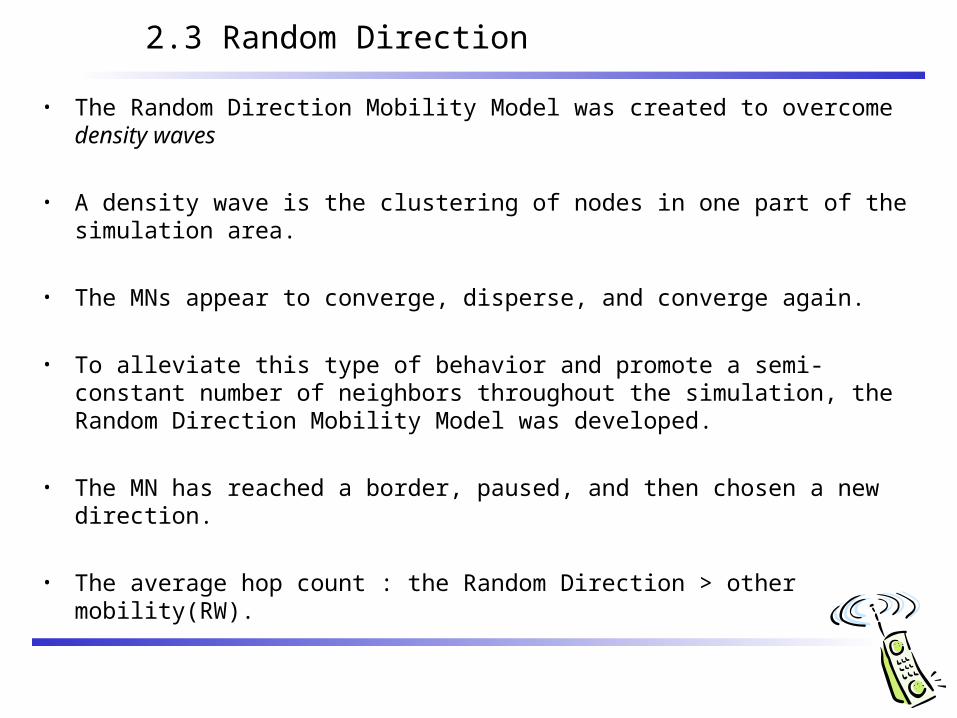
• The Random Direction Mobility Model was created to overcome density waves
• A density wave is the clustering of nodes in one part of the simulation area.
• The MNs appear to converge, disperse, and converge again.
• To alleviate this type of behavior and promote a semi-constant number of neighbors throughout the simulation, the Random Direction Mobility Model was developed.
• The MN has reached a border, paused, and then chosen a new direction.
• The average hop count : the Random Direction > other mobility(RW).
2.3 Random Direction
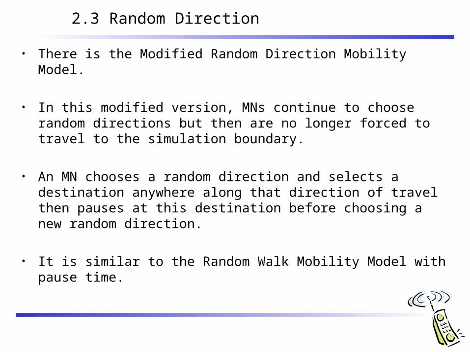
• There is the Modified Random Direction Mobility Model.
• In this modified version, MNs continue to choose random directions but then are no longer forced to travel to the simulation boundary.
• An MN chooses a random direction and selects a destination anywhere along that direction of travel then pauses at this destination before choosing a new random direction.
• It is similar to the Random Walk Mobility Model with pause time.

2.3 Random Direction
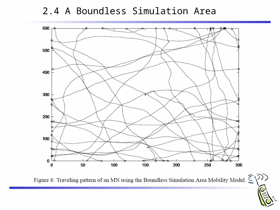
2.4 A Boundless Simulation Area
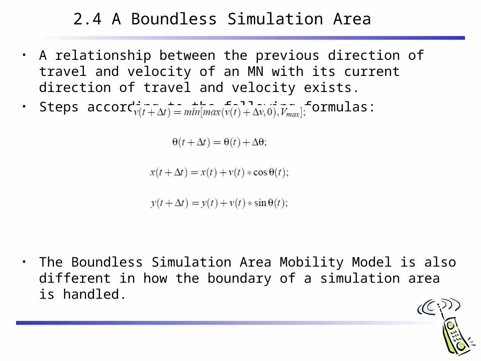
• A relationship between the previous direction of travel and velocity of an MN with its current direction of travel and velocity exists.
• Steps according to the following formulas:
• The Boundless Simulation Area Mobility Model is also different in how the boundary of a simulation area is handled.
2.4 A Boundless Simulation Area
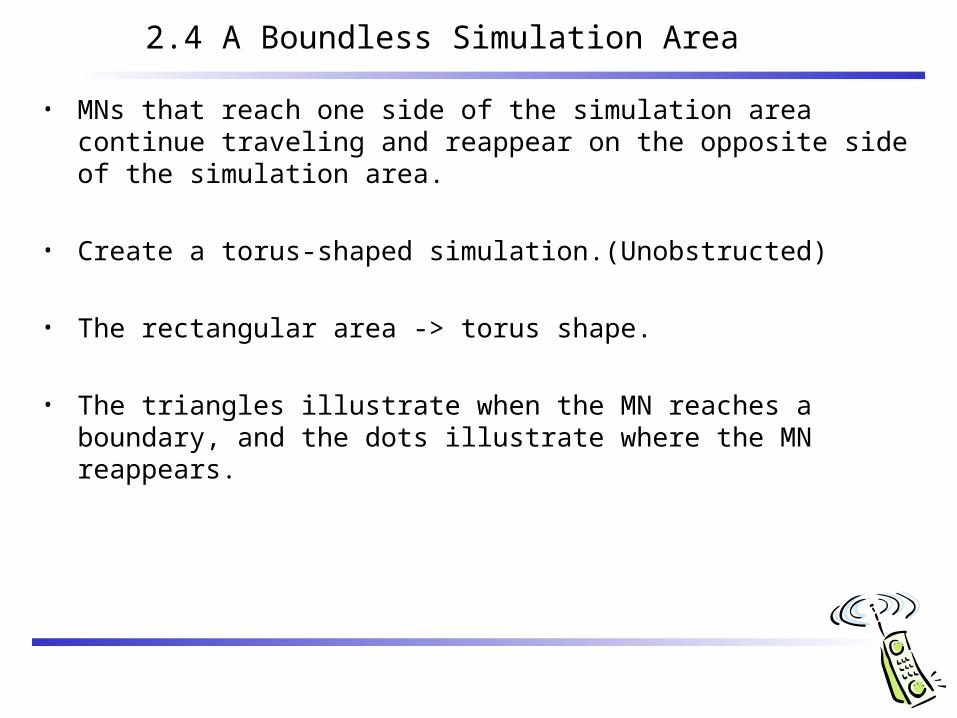
• MNs that reach one side of the simulation area continue traveling and reappear on the opposite side of the simulation area.
• Create a torus-shaped simulation.(Unobstructed)
• The rectangular area -> torus shape.
• The triangles illustrate when the MN reaches a boundary, and the dots illustrate where the MN reappears.

2.4 A Boundless Simulation Area
2.4 A Boundless Simulation Area

2.5 Gauss-Markov
• The Gauss-Markov Mobility Model was originally proposed for the simulation of a PCS.
• The Gauss-Markov Mobility Model was designed to adapt to different levels of randomness via one tuning parameter.
• Initially each MN is assigned a current speed and direction.• At fixed intervals of time, n, movement occurs by updating the speed
and direction of each MN.• The value of speed and direction at the nth instance is calculated using
the following equations.
2.5 Gauss-Markov
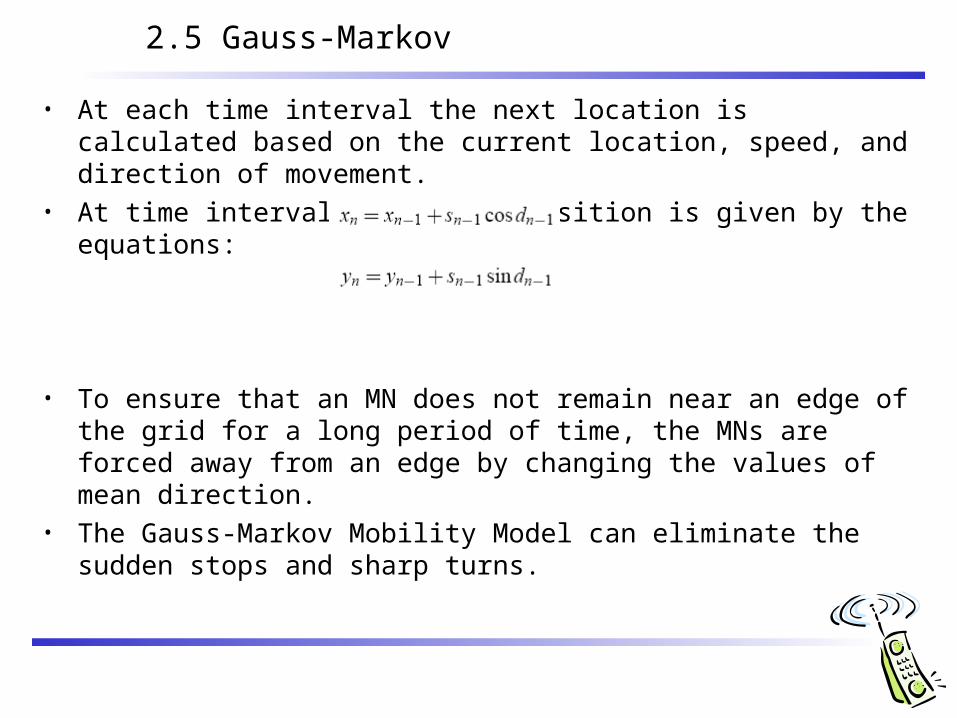
• At each time interval the next location is calculated based on the current location, speed, and direction of movement.
• At time interval n, an MN’s position is given by the equations:
• To ensure that an MN does not remain near an edge of the grid for a long period of time, the MNs are forced away from an edge by changing the values of mean direction.
• The Gauss-Markov Mobility Model can eliminate the sudden stops and sharp turns.

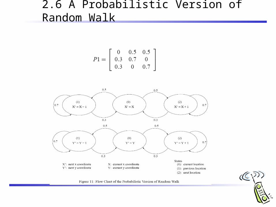
2.6 A Probabilistic Version of Random Walk
• Utilizes a probability matrix to determine the position of a particular MN in the next time step.
• Three different state for position x,y.• State 0 : the current(x or y) position of a given MN.• State 1 : the MN’s previous position.• State 2 : the next position if the MN continues to move in the same
direction.
• The probability matrix used is that an MN will go from state a to state b.• ( P(a,b)).
2.6 A Probabilistic Version of Random Walk

2.6 A Probabilistic Version of Random Walk
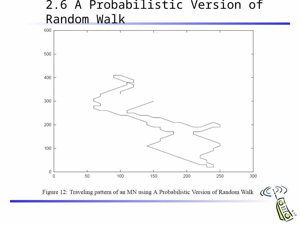
• With the values defined, an MN may take a step in any of the four possible direction.
• The probability of the MN continuing to follow the same direction is higher than The probability of the MN changing directions.
• Lastly, the values defined prohibit movements between the previous and next positions without passing through the current location.
• This model is realistic more than purely random movements but choosing appropriate values of P(a,b) may prove difficult.
• The MN moves in straight lines for periods of time and does not show the highly variable direction seen in the Random Walk Mobility Model.
2.6 A Probabilistic Version of Random Walk
2.7 City Section Mobility Model
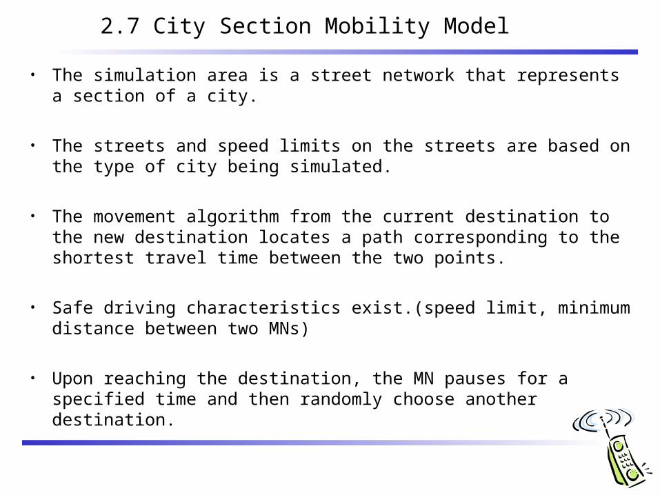
• The simulation area is a street network that represents a section of a city.
• The streets and speed limits on the streets are based on the type of city being simulated.
• The movement algorithm from the current destination to the new destination locates a path corresponding to the shortest travel time between the two points.
• Safe driving characteristics exist.(speed limit, minimum distance between two MNs)
• Upon reaching the destination, the MN pauses for a specified time and then randomly choose another destination.
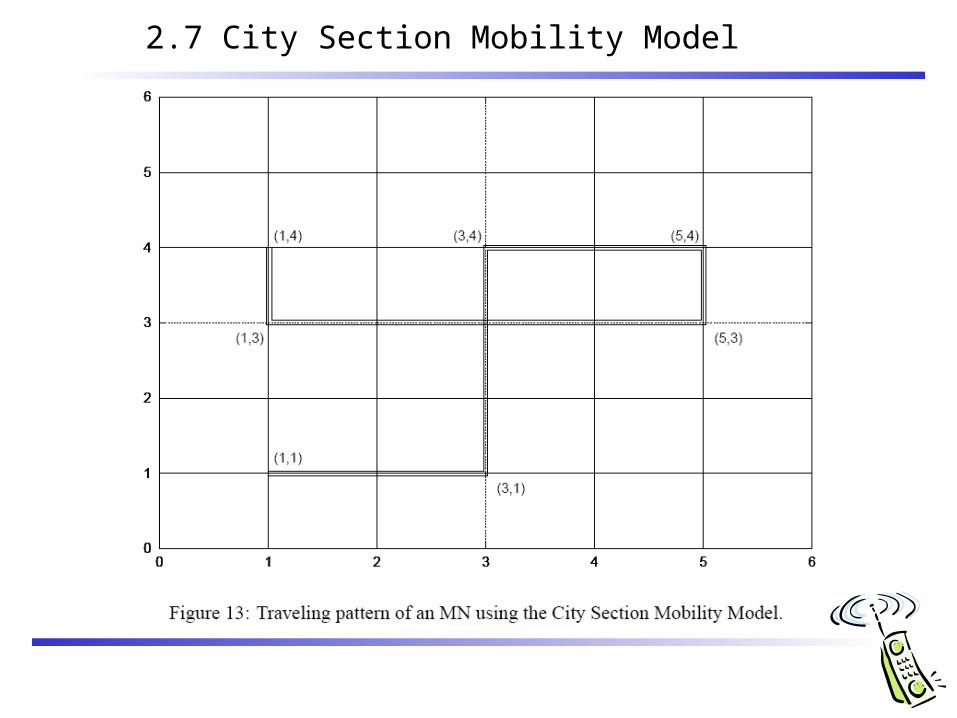
2.7 City Section Mobility Model
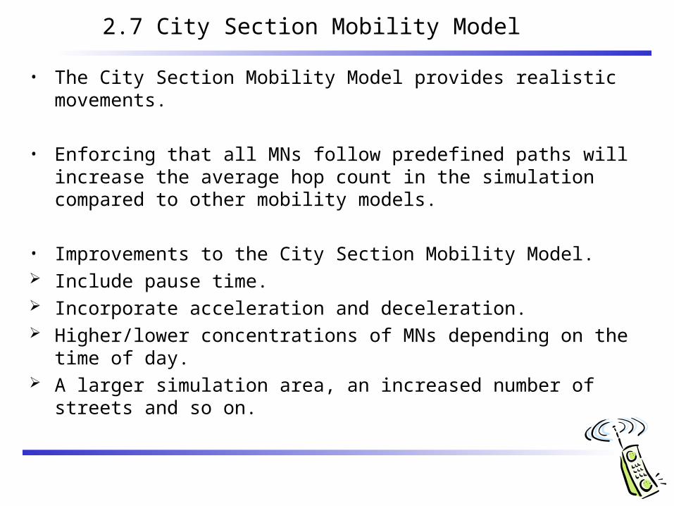
• The City Section Mobility Model provides realistic movements.
• Enforcing that all MNs follow predefined paths will increase the average hop count in the simulation compared to other mobility models.
• Improvements to the City Section Mobility Model. Include pause time. Incorporate acceleration and deceleration. Higher/lower concentrations of MNs depending on the time of day. A larger simulation area, an increased number of streets and so on.
2.7 City Section Mobility Model

3. Group Mobility Models
• Exponential Correlated Random Mobility Model.• Column Mobility Model.• Nomadic Community Mobility Model.• Pursue Mobility Model.• Reference Point Group Mobility Model.
The most general model is the Reference Point Group Mobility(RPGM) model
Column, Nomadic, and Pursue can be implemented as special cases of the RPGM model.
3.1 Exponential Correlated Random Mobility Model
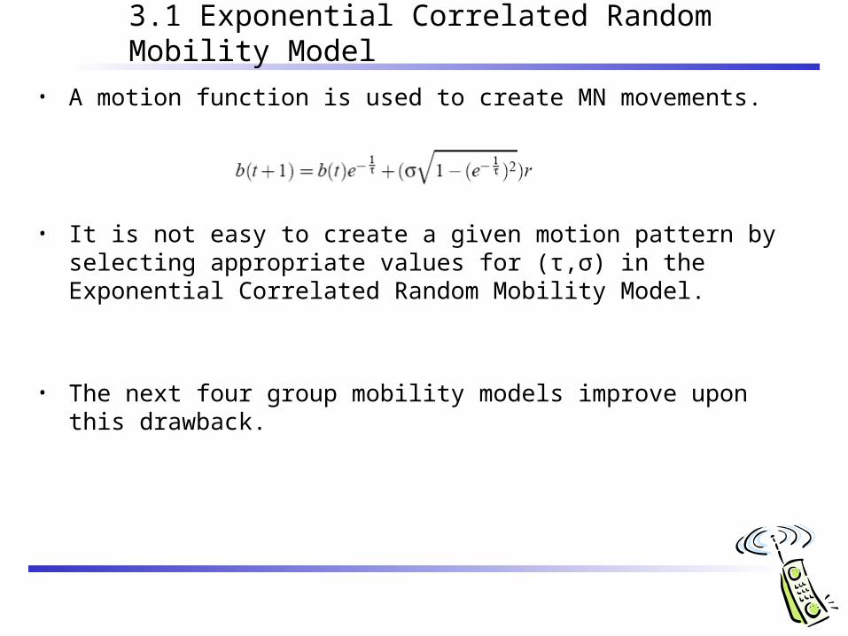
• A motion function is used to create MN movements.
• It is not easy to create a given motion pattern by selecting appropriate values for (τ,σ) in the Exponential Correlated Random Mobility Model.
• The next four group mobility models improve upon this drawback.

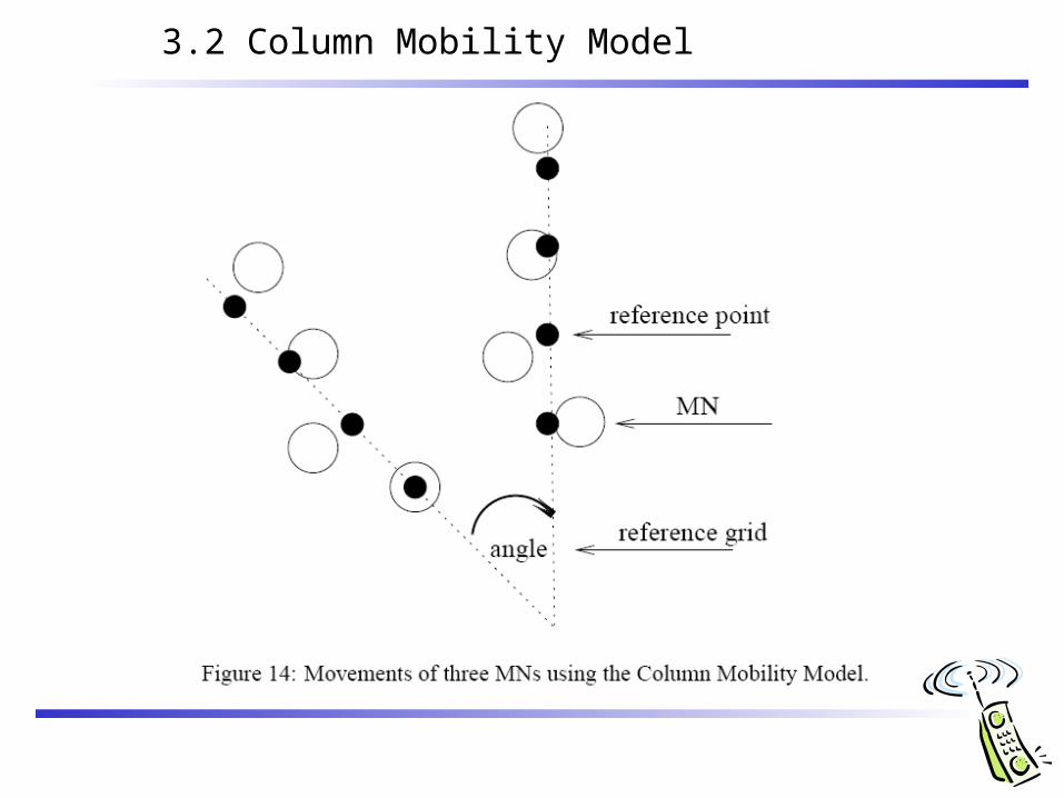
3.2 Column Mobility Model
• The Column Mobility Model proves useful for scanning or searching purposes.
• Represents a set of MNs that move around a given line(or column)• A slight modification of the Column Mobility Model allows the individual
MNs to follow one another.• Each MN is placed in relation to its reference point in the reference
grid.• The MN is then allowed to move randomly around its reference point .
• The new reference point for a given MN is defined as:

3.2 Column Mobility Model
• The MNs roam closely around their respective reference points.
• When the reference grid moves, the MNs follow the grid and then continue to roam around their respective reference points.
• These movement patterns for the Column Mobility Model using a variation of RPGM model implementation.
3.2 Column Mobility Model
3.3 Nomadic Community Mobility Model
• To represent groups of MNs that collectively move from on point to another.
• Within each community or group of MNs, individuals maintain their own personal “spaces”.
• Each MN uses an entity mobility model.(Random Walk) to roam around a given reference point.
• When the reference point changes , all MNs in the group travel to the new area defined by the reference point and then begin roaming around the new reference point .
• Compared to the Column Mobility Model, the MNs in the Nomadic Community Mobility model share a common reference point versus and individual reference point in a column.
• Less constrained in their movement around the defined reference point.

3.3 Nomadic Community Mobility Model
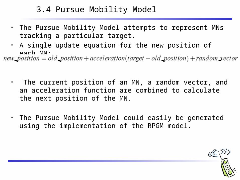
3.4 Pursue Mobility Model
• The Pursue Mobility Model attempts to represent MNs tracking a particular target.
• A single update equation for the new position of each MN:
• The current position of an MN, a random vector, and an acceleration function are combined to calculate the next position of the MN.
• The Pursue Mobility Model could easily be generated using the implementation of the RPGM model.

3.4 Pursue Mobility Model
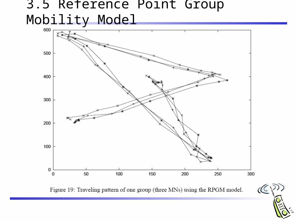
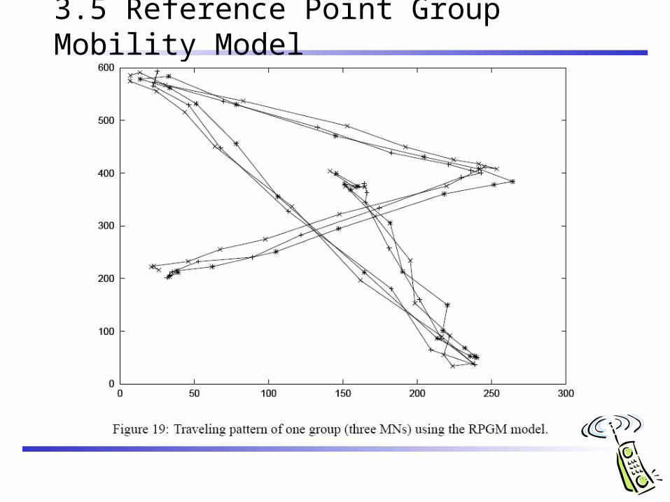
3.5 Reference Point Group Mobility Model
• Represents the random motion of a group of MNs as well as the random motion of each individual MN within the group.
• Group movements are based upon the path traveled by a logical center of the group.
• Individual MNs randomly move about their own pre-defined reference points.
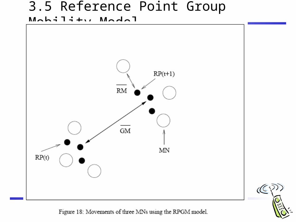
• the RPGM model uses a group motion vector GM to calculate each MN’s new reference point, RP(t +1), at time t +1.
• The length of RM is uniformly distributed within a specified radius centered at RP(t +1) and its direction is uniformly distributed between 0 and 2π.
3.5 Reference Point Group Mobility Model
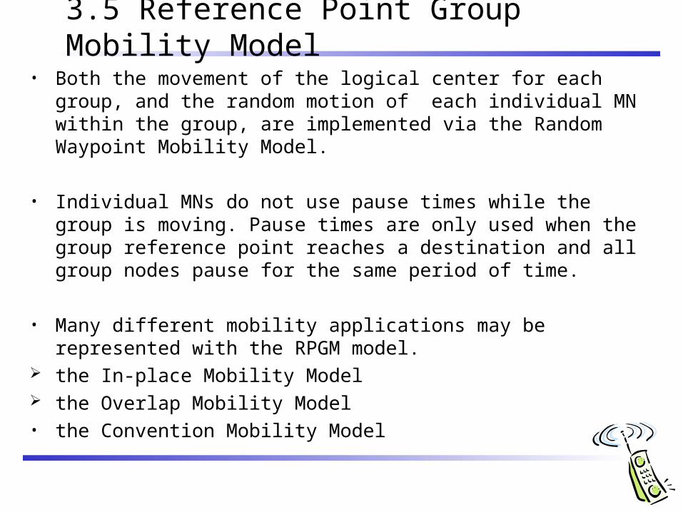
• Both the movement of the logical center for each group, and the random motion of each individual MN within the group, are implemented via the Random Waypoint Mobility Model.
• Individual MNs do not use pause times while the group is moving. Pause times are only used when the group reference point reaches a destination and all group nodes pause for the same period of time.
• Many different mobility applications may be represented with the RPGM model.
the In-place Mobility Model the Overlap Mobility Model• the Convention Mobility Model
3.5 Reference Point Group Mobility Model
3.5 Reference Point Group Mobility Model
3.5 Reference Point Group Mobility Model

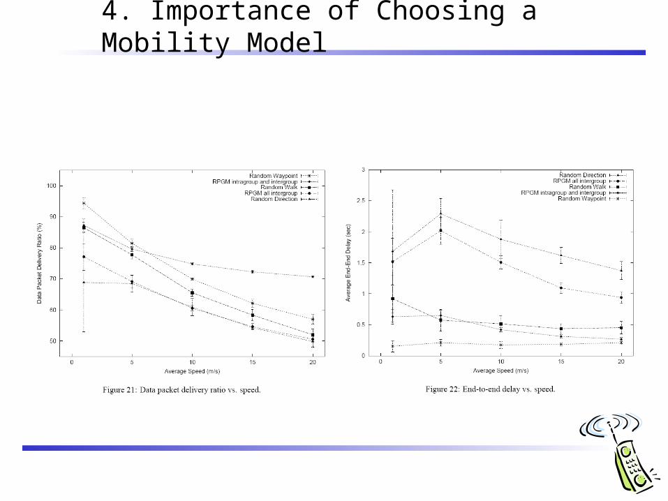
4. Importance of Choosing a Mobility Model
• The choice of a mobility model can have a significant effect on the performance investigation of an ad hoc network protocol.
• Use ns-2.• 50MNs.• 100m transmission range.• Use DSR.• DSR performs well in many of the performance evaluations of unicast
routing protocols.• 2010seconds(1000- 2000).• 20 CBR.• 64 byte packet size.• The initial location of the MNs are random.
4. Importance of Choosing a Mobility Model

4. Importance of Choosing a Mobility Model
the Random Waypoint Mobility Model has the highest data packet delivery ratio, the lowest end-to-end delay, and the lowest average hop count compared to the Random Walk Mobility Model and Random Direction Mobility Model.
• MNs using the Random Waypoint Mobility Model are often traveling through (or to) the center of the simulation area.
• the Random Direction Mobility Model has each MN move to the border of the simulation area before changing direction.
The confidence intervals of the Random Walk Mobility Model and Random Direction Mobility Model are the largest ; more variation in movement patterns exist in these two mobility models.
The data packet delivery ratio is not high than expected in case of RPGM; since 50% of the packets are transmitted between groups, these packets are sometimes dropped due to the transient partitions that occur.

4. Importance of Choosing a Mobility Model
5. Conclusions
• The performance of a wireless adhoc network protocol can vary significantly with different mobility models
• The performance of an ad hoc network protocol can vary significantly when the same mobility model is used with different parameters.
• The selection of a mobility model may require a data traffic pattern which significantly influences protocol performance.
• The performance of an ad hoc network protocol should be evaluated with the mobility model that most closely matches the expected real-world scenario.
• If the expected real-world scenario is unknown, then researchers should make an informed choice about the mobility model to use.

Graph-Based Mobility Model for Mobile Ad Hoc Network Simulation
1. Introduction
Conventional scenarios in MANET(A mobile ad hoc network) simulation use random mobility models.
However, mobile nodes in the real world, such as human beings or vehicles, do not move randomly.
Introduce a novel graph-based mobility model that reflects the spatial constraints of the real world.
Compare the performance of three commonly used ad-hoc routing protocols both using the graph-based model and the random walk model.
1. Introduction
250m transmission range , lower transmission ranges from 10m to 150
m.
Section 2 - Introduces a graph-based mobility model.
Section 3 - A brief description of the investigated routing protocols.
Section 4 - Describe the simulation methology and the simulation results.
Section 5 - Related work.
Section 6 – conclusions and further work.
2. Graph-Based Mobility Model
Use a graph to model the movement constraints imposed by the infrastructure.
Vertices – locations , Edges – the connections between locations
Each mobile node is initialized at a random vertex in the graph.
Vertex is selected randomly as its destination.
Shortest possible path
Short pause for a randomly selected period and picks out another destination.
This model provides a realistic balance between completely deterministic and completely random mobility models.
2. Graph-Based Mobility Model
2. Graph-Based Mobility Model
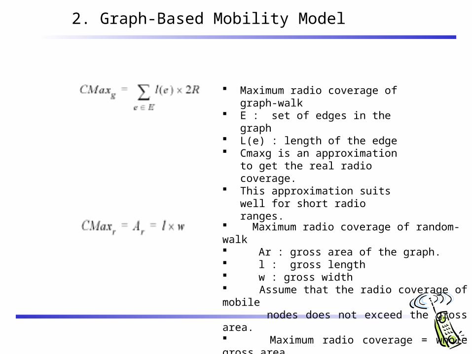
Maximum radio coverage of graph-walk
E : set of edges in the graph L(e) : length of the edge Cmaxg is an approximation to get
the real radio coverage. This approximation suits well for
short radio ranges.
Maximum radio coverage of random-walk Ar : gross area of the graph. l : gross length w : gross width Assume that the radio coverage of mobile nodes does not exceed the gross area. Maximum radio coverage = whole gross area
2. Graph-Based Mobility Model
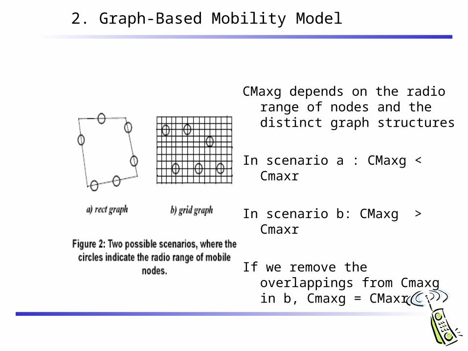
CMaxg depends on the radio range of nodes and the distinct graph structures
In scenario a : CMaxg < Cmaxr
In scenario b: CMaxg > Cmaxr
If we remove the overlappings from Cmaxg in b, Cmaxg = CMaxr
2. Graph-Based Mobility Model
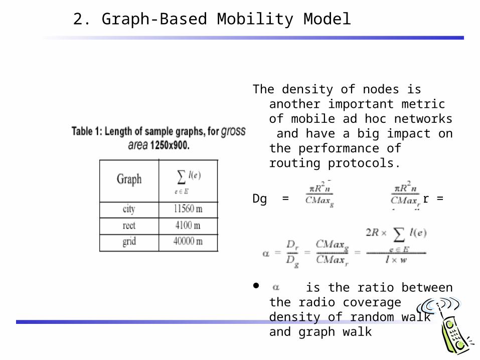
The density of nodes is another important metric of mobile ad hoc networks and have a big impact on the performance of routing protocols.
Dg = , Dr =
is the ratio between the radio coverage density of random walk and graph walk
2. Graph-Based Mobility Model
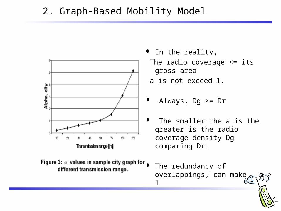
In the reality,
The radio coverage <= its gross area
a is not exceed 1.
Always, Dg >= Dr
The smaller the a is the greater is the radio coverage density Dg comparing Dr.
The redundancy of overlappings, can make , a > 1

3. Description of Routing Protocols
DSDV(Destination Sequenced Distance Vector)
• DSR(Dynamic Source Routing)
• AODV(Ad hoc On Demand Distance Vector)
DSDV is a proactive protocol.
DSR and AODV are reactive protocol.
AODV is based on traditional distance vector mothod.
DSR is a source routing protocol.
3.1 Destination-Sequenced Distance-Vector
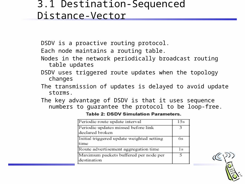
DSDV is a proactive routing protocol.Each node maintains a routing table. Nodes in the network periodically broadcast routing table
updatesDSDV uses triggered route updates when the topology changesThe transmission of updates is delayed to avoid update storms.The key advantage of DSDV is that it uses sequence numbers to
guarantee the protocol to be loop-free.

3.2 Dynamic Source Routing(DSR)
DSR is a reactive routing protocol.Route Discovery , Route Maintenance.If a node wants to find a route to another node, it uses the route
discovery mechanism to flood a Route Request(RREQ) packet.
If a route to the destination is found, a Route Reply(RREP) packet will be sent back to the source node by unicast.
Each intermediate node that forwards the RREP message also learns this route by caching it in its routing table.
3.3 Ad Hoc on Demand Distance Vector
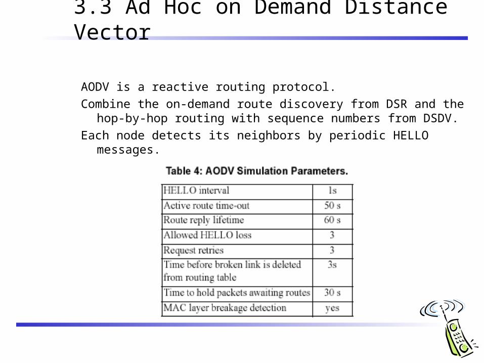
AODV is a reactive routing protocol.
Combine the on-demand route discovery from DSR and the hop-by-hop routing with sequence numbers from DSDV.
Each node detects its neighbors by periodic HELLO messages.

4. Simulation
Introduce simulation environment.
Analyze the simulation results of both graph walk model and
random walk model.
Brief summary of the simulation.

4.1 Simulation Environment
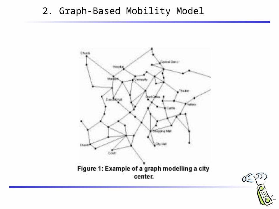
Based on the city scenario in Section 2. The city center was modeled as a graph.( Figure. 1) 115 vertices, 150 edges , 1250m X 900m. Each node moves from one randomly chosen location to the next on a
shortest path. After reaching a destination a pause time( Tstaymin< T < Tstaymax)
was chosen befor moving towards the next destinations. NS2 with the CMU extension. Every node has a minimum nad maximum speed(Vmin, Vmax) IEEE 802.11

4.1 Simulation Environment
4.2 Simulation Results
Compare simulation results of the three routing protocols.
Compare the performance of protocols in terms of the average end-to-end delay, packet delivery rate and routing protocol packet overhead.
Tested on random walk as well as graph walk, and also with a variety of radio ranges.
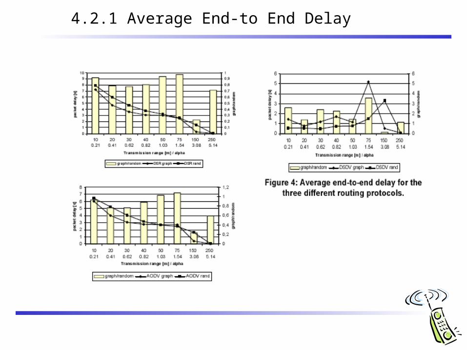
4.2.1 Average End-to End Delay

4.2.1 Average End-to End Delay
The average packet delay of DSDV in the graph walk model than in random walk model.
Spatial constraint of graph forced more hops to be used on detours along the graph than in random walk.
DSR, AODV achieve lower delay in graph walk than in random walk even with more hops needed.
While the delay of AODV, DSR is mainly caused by the buffering of undeliverable packets, the number of hops plays a critical role in DSDV .
When a < 1 , Cmaxr > Cmaxg -> higher radio coverage density of nodes in graphwalk than in random walk.
The higher density of nodes increases the probability of finding relay nodes to forward the packets.
When a > 1, the radio coverage density in graph walk is very close to random walk, all the three protocols do not show a significant difference between both models.
4.2.2. Packet Delivery Rate
4.2.2. Packet Delivery Rate
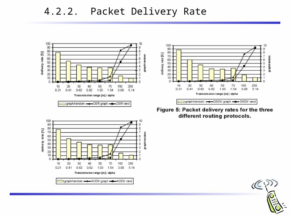
For all three candidates the packet delivery rate grows exponentially for the transmission ranges up to 75m.
All protocols deliver more packets in the graph walk than in random walk.
AODV and DSR have higher delivery rates compared to DSDV.
The lowest delivery rates are observed in the random walk senario of DSDV.
Both DSR and AODV in the graph scenario achieve highest delivery rate.
When the a value is significantly greater than 1, especially at 250m radio range, the packet delivery rate for all three protocols do not have evident difference in the graph walk model comparing to the random walk model.

4.2.3. Routing Protocol Packet Overhead

4.2.3. Routing Protocol Packet Overhead
None of the three protocols show large differences in routing protocol packet overhead between graph walk and random walk models.
The DSDV protocol has an approximately constant overhead for transmission ranges up to 75m and increases slightly for higher ranges.
AODV shows an approximately linear increase of the protocol overhead in short ranges for both graph and random walk.
Within the lower radio ranges the graph walk has a higher overhead than random walk.
The routing packet overhead decreases in both DSR and AODV with high radio ranges.
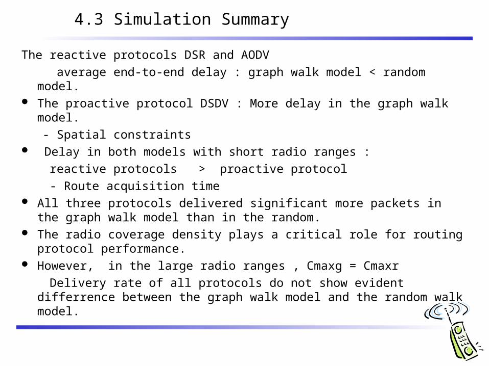
4.3 Simulation Summary
The reactive protocols DSR and AODV
average end-to-end delay : graph walk model < random model. The proactive protocol DSDV : More delay in the graph walk model.
- Spatial constraints Delay in both models with short radio ranges :
reactive protocols > proactive protocol
- Route acquisition time All three protocols delivered significant more packets in the graph walk
model than in the random. The radio coverage density plays a critical role for routing protocol
performance. However, in the large radio ranges , Cmaxg = Cmaxr
Delivery rate of all protocols do not show evident differrence between the graph walk model and the random walk model.

4.3 Simulation Summary
Routing packet overhead(DSR) with short radio ranges:
Graph Model = Random Model Routing packet overhead(DSR) with large radio ranges:
Graph Model < Random Model Routing packet overhead(AODV) with short radio ranges:
Graph Model > Random Model The reactive protocols DSR and AODV achieved less overhead with
increasing radio range whereas the proactive protocol DSDV got more overhead.

5. Related Work
Graph walk model, Considered a variety of small radio ranges
Johnasson introduced three additional scenarios:
Conference, Event Coverage, Disaster Area.
Obstacle-approach
Obstacle-approach was not to improve the modelling of the movement
of mobile nodes.
Graph-approach to model the movement of mobile nodes.

6. Conclusion
The spatial constraints have a big impact on the performance of mobile ad hoc routing.
Routing protocols performed quite differently in this graph walk model from the random walk model.
For the near future, extend our graph model by including obstacles.
Plan to include movement profiles of distinct nodes in our model.
Plan to evaluate the location aware routing protocols like LAR and GPSR with graph walk model in the future.

Weighted Waypoint Mobility Model and Its Impact on Ad Hoc Networks
Able-to-skip

Motivation
•Pedestrians on campus do not move randomly. They pick their destinations based on preferences related to daily tasks. (e.g. going to class or lunch.)
•Generally people tend to stay at a building longer than travel between buildings (low move-stop ratio).
•Most current mobility models (e.g. RWP) fail to capture mobility preferences and have high move-stop ratio.
•Objective: Design a more realistic mobility model to better model mobility pattern for campus environment.
•Approach: Collect mobility traces on campus via student surveys, build WWP model, and study its characteristics and impact on networks via simulation

•We categorize the buildings on campus into 3 types: (I). classrooms, (II). libraries, (III). cafeterias. There are also (IV). other area on campus and (V). off-campus area. These are 5 destination categories in our survey and mobility model.•Mobile node (MN) chooses its next destination category based on weights determined by its current location (location dependent) and time of the day (time dependent). The weights are estimated from survey data.•Distribution of pause time and wireless network usage (flow-initiation prob. and distribution of duration) at locations are determined by the survey.•Facts about the survey:
Weighted Way Point Model
Total survey countsDuration of
surveyTime segments of survey
processing
268Mar. 22 – Apr. 16
20049AM-1PM and 1PM-5PM
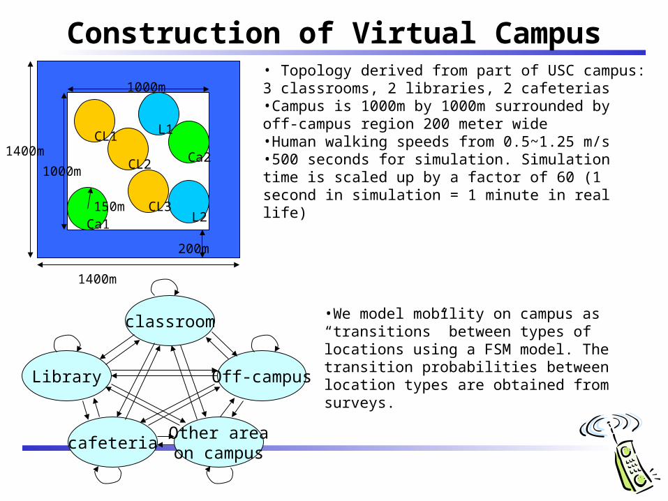
Construction of Virtual Campus• Topology derived from part of USC campus: 3 classrooms, 2 libraries, 2 cafeterias•Campus is 1000m by 1000m surrounded by off-campus region 200 meter wide •Human walking speeds from 0.5~1.25 m/s•500 seconds for simulation. Simulation time is scaled up by a factor of 60 (1 second in simulation = 1 minute in real life)
classroom
Off-campus
Other areaon campus
cafeteria
Library
200m
1400m
1400m
1000m
1000m
CL1
CL2
CL3
L1
L2Ca1
Ca2
150m
•We model mobility on campus as “transitions” between types of locations using a FSM model. The transition probabilities between location types are obtained from surveys.
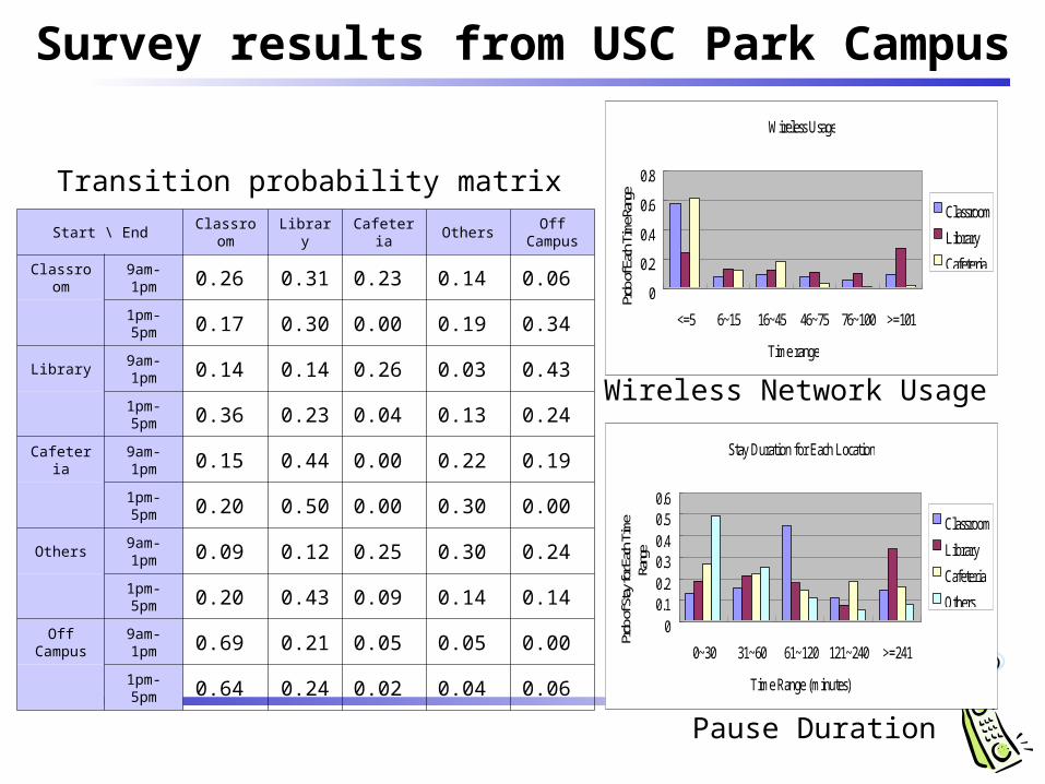
Survey results from USC Park Campus
Transition probability matrix
Stay Duration for Each Location
00.10.20.30.40.50.6
0~30 31~60 61~120 121~240 >=241
Time Range (minutes)
Prob
of St
ay fo
r Each
Tim
eRa
nge
Classroom
Library
Cafeteria
Others
Wireless Usage
0
0.2
0.4
0.6
0.8
<=5 6~15 16~45 46~75 76~100 >=101
Time range
Prob
of E
ach T
ime R
ange
Classroom
Library
Cafeteria
Wireless Network Usage
Pause Duration
Start \ EndClassroo
mLibrary
Cafeteria
OthersOff
Campus
Classroom
9am-1pm 0.26 0.31 0.23 0.14 0.06
1pm-5pm 0.17 0.30 0.00 0.19 0.34
Library9am-1pm 0.14 0.14 0.26 0.03 0.43
1pm-5pm 0.36 0.23 0.04 0.13 0.24
Cafeteria9am-1pm 0.15 0.44 0.00 0.22 0.19
1pm-5pm 0.20 0.50 0.00 0.30 0.00
Others9am-1pm 0.09 0.12 0.25 0.30 0.24
1pm-5pm 0.20 0.43 0.09 0.14 0.14
Off Campus
9am-1pm 0.69 0.21 0.05 0.05 0.00
1pm-5pm 0.64 0.24 0.02 0.04 0.06

(1) Uneven spatial distribution (Clustering) MNs choose the locations as its destination with higher probability and stay
there longer. Most of the MNs are within some locations rather than at other area on the virtual campus.
(2) Time-variant spatial distribution No “steady state” of MN distribution- before the node density converges, the
transition matrix changes, and the node distribution will move toward another potential steady state, which it may never reach.
(3) Less mobile than RWP For typical parameters used for RWP model, the move-stop ratio is much
higher than the survey-based WWP model.
Properties of WWP model
0
0.0001
0.0002
0.0003
0.0004
0.0005
0.0006
0.0007
0 100 200 300 400 500 600
time
Node
densi
ty (#
of no
de/lo
cation
area)
Class ALibrary ACafé AOthersOff campus
Model and parameters Move-stop ratio
WWP with empirical pause time from survey, speed=[30,75] (m/s)
0.12
RWP with pause time = [0,480] (s) speed=[30,75] (m/s)
0.08
RWP with pause time=[0,100] (s) speed=[2,50] (m/s)
0.99

Impact of WWP model
# of FLOWs generated by each model
0100200300400500600
50 100 150 200 250 300 350 400 450 500 550
Number of MNs
Tota
l Flo
ws
Gen
erat
ed
WWP
RWP
Congested Ratio for each model
0%
20%
40%
60%
80%
100%
50 100 150 200 250 300 350 400 450 500 550
Number of MNs
Conges
ted R
atio
WWP
RWP
# of flows v.s. Congested Ratio
0%
20%
40%
60%
80%
100%
0 200 400 600
# of Flows
Congested R
atio
WWP
RWP
Higher congestion ratio of WLAN in buildings
Lower Route Discovery Success Ratein MANET due to Network Partition
0.00%20.00%40.00%60.00%80.00%
100.00%
Location Relationship
Avg
Suc
cess
Rat
e
Near
Far
Near Locations
Far Locations

Summary
•Weighted Way Point model is proposed to better capture features of pedestrian mobility on campus.
•Applying WWP model on the virtual campus shows its effects on MN behavior, including (I).Uneven spatial distribution (II).No steady state and (III).Low move-stop ratio.
•Impact of WWP on wireless networks (WLAN and ad hoc networks) shows higher local congestion in WLAN and lower success rate of route discovery in MANET than RWP model.
Future Works
•Look for systematic method to correlate AP-traces with MN mobility.
•Look for meaningful statistical metrics (e.g. average percentage of APs visited by a MN) to compare/distinguish mobility patterns in different campus/environment.
•Establish a systematic method to create “mobility matrix” from observation of flux at some nodes. [Ref] http://nile.usc.edu/~helmy/mobility-trace
Group and Swarm mobility models for ad hoc network scenarios using virtual tracks
1. Introduction
In most simulation experiments, node movement is modeled as an independent random walk. (Random WayPoint Mobility)
In real military scenariois, node mobility is not always independent.
(Group mobility) “Virtual track” based group mobility model(VT model)
- a certain number of “switch stations” are randomly placed in the field.
- All interconnected by “virtual tracks”
- Groups move along the virtual tracks towards the stations.
- At a station, a group can then be split into multiple groups heading to different stations.
- Group entering the same station may also merge
- The individually moving nodes are random moves without constraint of the virtual tracks.
1. Introduction
Compare VT mobility model with the random waypoint mobility
Section 2 : Briefly review related research in the area of mobility modeling.
Section 3 : overview of the proposed mobility model
Section 4 : details of the schemes
Section 5 : Intensive simulation investigation of the mobility model
Section 6 : Conclusion

2. Related work
Random Waypoint(RWP) model
Random Walk mobility model
Reference Point Group Mobility(RPGM) Model
Obstacle Mobility model
Manhattan mobility model
All existing mobility models don’t pay much attention on the group movement and dynamic group split and merge in reality.
VT mobility model is a suitable model to simulate the heterogeneous mobility scenario.
3. Overview of the virtual track based Group mobility model
• “virtual tracks”• “switch stations”• Split and merge at switch stations with probabilities.• Internal random mobility within the scope of a group.• Speed ( Minimum < s < Maximum )• Class of mobile nodes(pedestrians, cars, UGVs and UAVs)• Randomly and individually moving modes, static nodes(such
as sensors)• Non-grouped nodes• VT mobility model is suitable for both military and urban
environment.

3. Overview of the virtual track based Group mobility model

4. Design of virtual track based mobility model
4.1 Defining Switch Stations and Virtual Tracks The user can specify the number of stations in the scenario. Randomly choose the positions for these stations in the field. Define a maximum length of the track The track width can be user specified or randomly chosen, Users can specify the positions of switch stations and the tracks
connecting these stations.

4. Design of virtual track based mobility model
Initial Node Distribution and Group Affiliation The group nodes are initially distributed along the virtual tracks Individual nodes are initially distributed in the whole field without
considering the tracks.
4. Design of virtual track based mobility model
Group Mobility under Constraint of Tracks Initially, nodes in the same group are placed on the same track. Select the same switch station at either end of the track. The group as a whole will move towards it. Random waypoint mobility with two conditions for selecting the
intermediate points
1. An intermediate point must be closer to the destination than previous points.
2. The point must be on the same track. The group movements are applied to all nodes within the group. Each node in the group can also have a small internal mobility under
the constraints of the group and tracks.
4. Design of virtual track based mobility model
Group Split/Merge at the Switch Station Groups split and merge happen at the switch stations. Group stability threshold value. Check whether its stability value is beyond its group stability threshold
value. If it is true, A group split happens. When several group arrive at the same station and select the same
track for the next movement, they will be merged.
4. Design of virtual track based mobility model
4.5 Random and Individual Nodes Static nodes , individually moving nodes Static nodes are randomly or uniformly distributed within the whole
field and have no mobility. Individually moving modes have random mobility within the whole field
without track constraints. Using RWP model.
5. Simulation Evaluation
5.1 Simulation Platform Implemented in the QualNet network simulator. Compared VT mobility model with RWP model using AODV Simulation topology : Partial LA highway map 11 intersections. 2200m X 2800m 150 nodes , 4 groups 60 CBR flows , 487.50Kbps.

5. Simulation Evaluation

5. Simulation Evaluation
5.2 Performance with Mobile Groups Only

5. Simulation Evaluation
• Overall performance under group mobility is worse than that under random mobility.• When nodes are moving in groups, the connectivity within a group is strengthened but the connectivity across groups will be typically weaker.• RWP model when the modes in reality move in groups will give inaccurate.
5. Simulation Evaluation
5.3 Impact of Individual Random Moving and Static Nodes
Study the performance under VT mobility model with individual nodes and static modes.
Examine whether the individual nodes and static nodes can help maintain rich connectivity among the groups
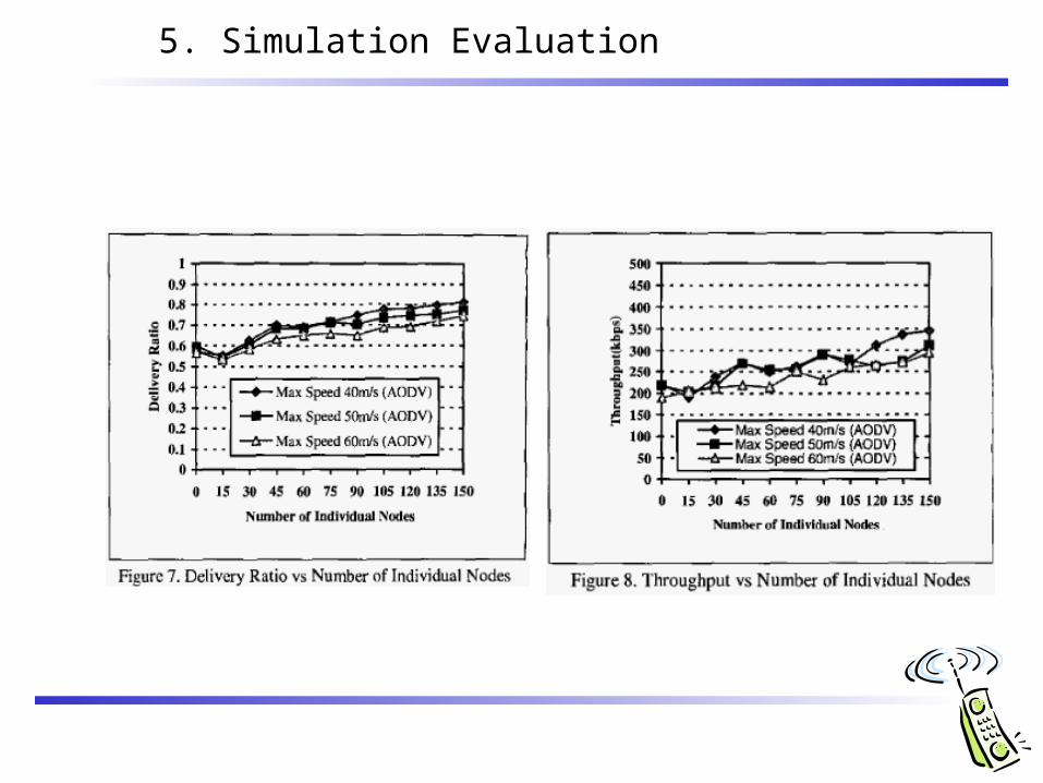
150 nodes, Three different max speeds(40, 50 , 60 m/s) AODV routing protocol is used.
5. Simulation Evaluation
5. Simulation Evaluation
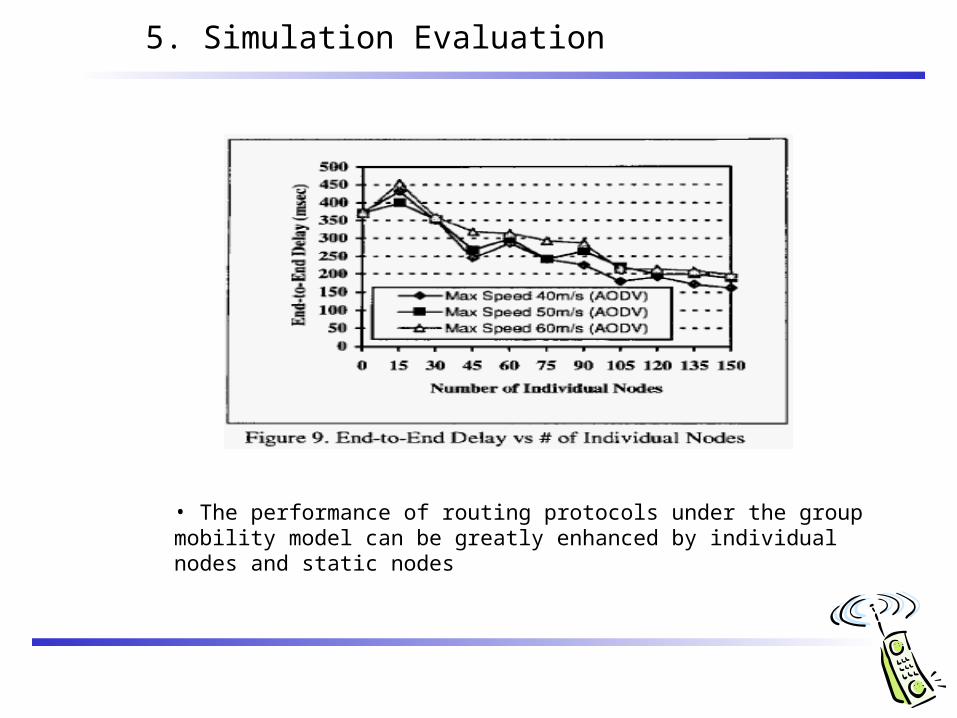
• The performance of routing protocols under the group mobility model can be greatly enhanced by individual nodes and static nodes
6. Conclusion
• Proposed a Virtual Track based group mobility model(VT model).• Introduce the concept of “Switch Stations” and “Virtual Tracks”• Individually moving modes and static nodes are also included in the
model.• The simulation results had significant impact on the performance
evaluation of network protocols such as routing protocols.
Related Documents