EE3J2 Data Mining Slide 1 EE3J2 Data Mining Lecture 10 Statistical Modelling Martin Russell

Slide 1 EE3J2 Data Mining EE3J2 Data Mining Lecture 10 Statistical Modelling Martin Russell.
Dec 19, 2015
Welcome message from author
This document is posted to help you gain knowledge. Please leave a comment to let me know what you think about it! Share it to your friends and learn new things together.
Transcript
EE3J2 Data MiningSlide 1
EE3J2 Data Mining
Lecture 10Statistical Modelling
Martin Russell
EE3J2 Data MiningSlide 2
Objectives
To review basic statistical modelling To review the notion of probability distribution To review the notion of probability distribution To review the notion of probability density function To introduce mixture densities To introduce the multivariate Gaussian density
EE3J2 Data MiningSlide 3
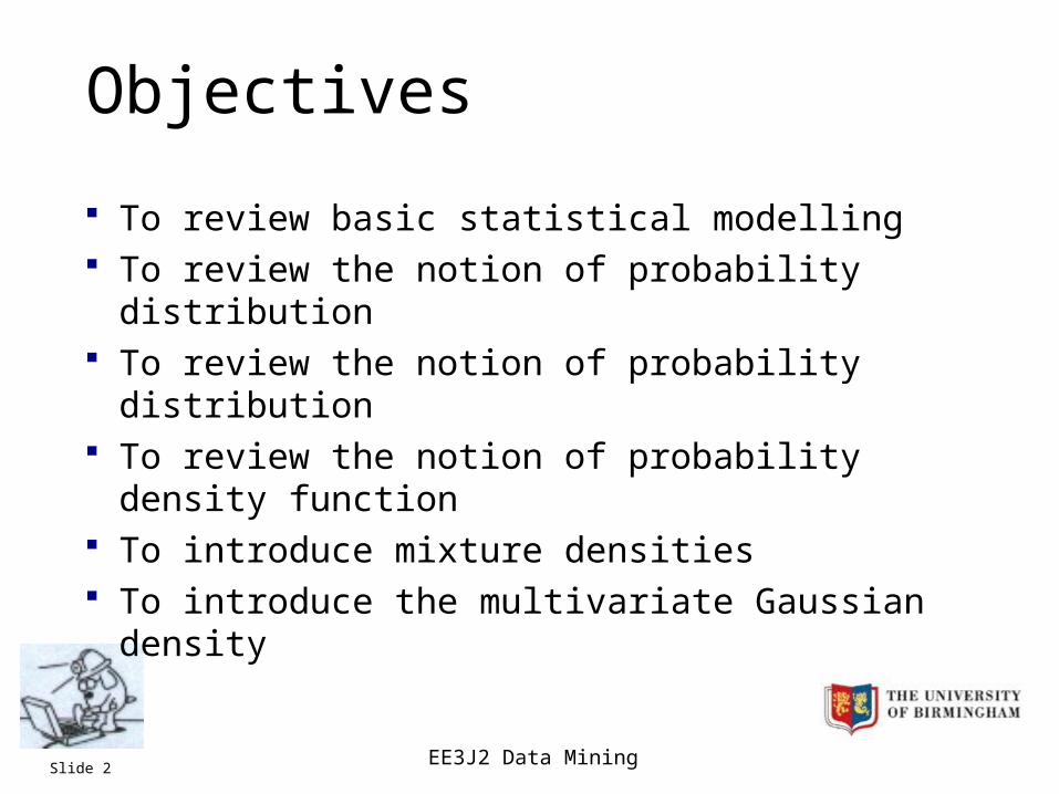
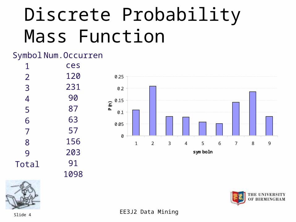
Discrete variables
Suppose that Y is a random variable which can take any value in a discrete set X={x1,x2,…,xM}
Suppose that y1,y2,…,yN are samples of the random variable Y
If cm is the number of times that the yn = xm then an estimate of the probability that yn takes the value xm is given by:
N
cxyPxP m
mnm
EE3J2 Data MiningSlide 4
Discrete Probability Mass Function
0
0.05
0.1
0.15
0.2
0.25
1 2 3 4 5 6 7 8 9
symbol n
P(n
)
Symbol123456789
Total
Num.Occurrences12023190876357
15620391
1098
EE3J2 Data MiningSlide 5
Continuous Random Variables
In most practical applications the data are not restricted to a finite set of values – they can take any value in N-dimensional space
Simply counting the number of occurrences of each value is no longer a viable way of estimating probabilities…
…but there are generalisations of this approach which are applicable to continuous variables – these are referred to as non-parametric methods
EE3J2 Data MiningSlide 6
Continuous Random Variables
An alternative is to use a parametric model In a parametric model, probabilities are defined by a
small set of parameters Simplest example is a normal, or Gaussian model A Gaussian probability density function (PDF) is
defined by two parameters – its mean and variance
EE3J2 Data MiningSlide 7
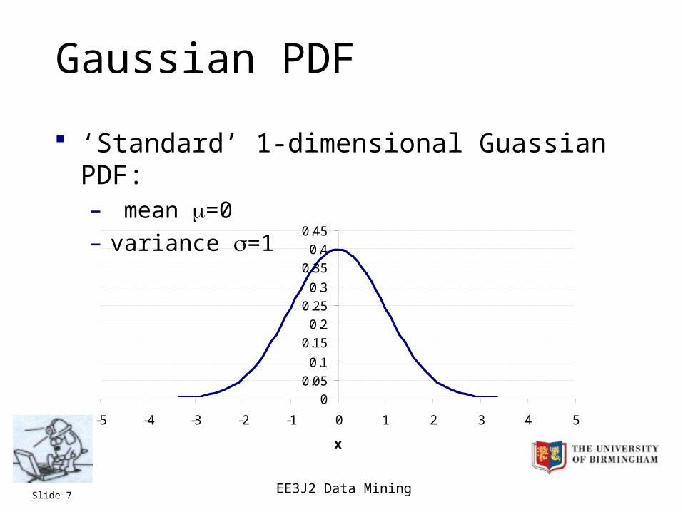
Gaussian PDF
‘Standard’ 1-dimensional Guassian PDF:– mean =0
– variance =1
0
0.05
0.1
0.15
0.2
0.25
0.3
0.35
0.4
0.45
-5 -4 -3 -2 -1 0 1 2 3 4 5
x
EE3J2 Data MiningSlide 8
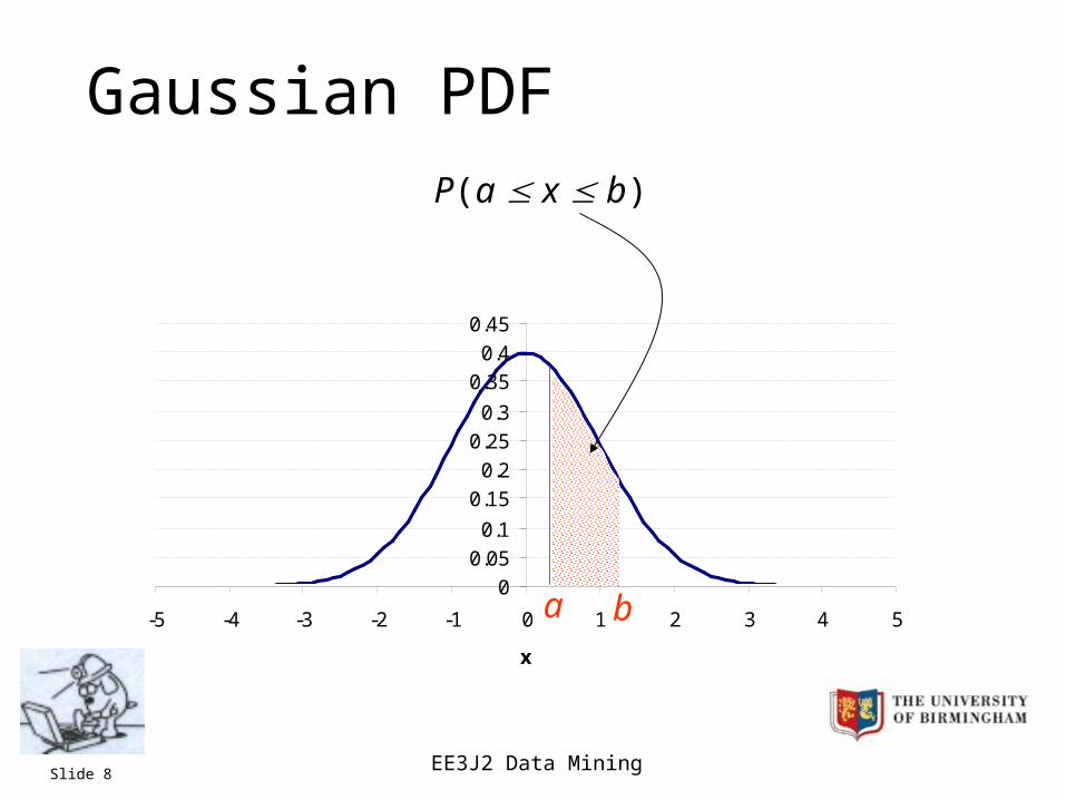
Gaussian PDF
0
0.05
0.1
0.15
0.2
0.25
0.3
0.35
0.4
0.45
-5 -4 -3 -2 -1 0 1 2 3 4 5
x
a b
P(a x b)
EE3J2 Data MiningSlide 9
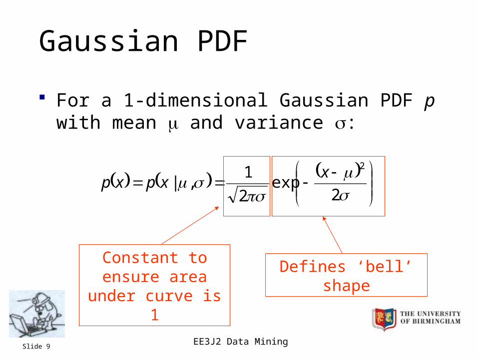
Gaussian PDF
For a 1-dimensional Gaussian PDF p with mean and variance :
2exp
2
1,|
2xxpxp
Constant to ensure area under curve is 1
Defines ‘bell’ shape
EE3J2 Data MiningSlide 10
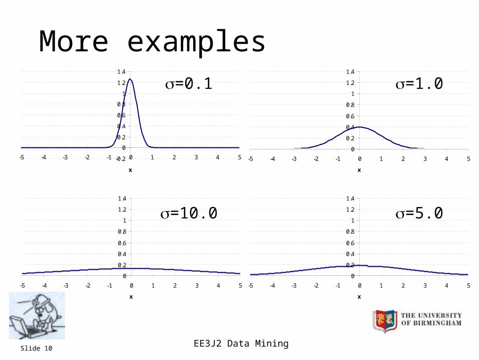
More examples
-0.2
0
0.2
0.4
0.6
0.8
1
1.2
1.4
-5 -4 -3 -2 -1 0 1 2 3 4 5
x
0
0.2
0.4
0.6
0.8
1
1.2
1.4
-5 -4 -3 -2 -1 0 1 2 3 4 5
x
=0.1 =1.0
0
0.2
0.4
0.6
0.8
1
1.2
1.4
-5 -4 -3 -2 -1 0 1 2 3 4 5
x
0
0.2
0.4
0.6
0.8
1
1.2
1.4
-5 -4 -3 -2 -1 0 1 2 3 4 5
x
=10.0 =5.0
EE3J2 Data MiningSlide 11
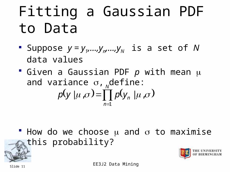
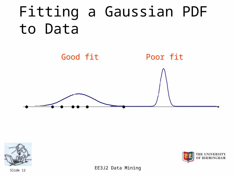
Fitting a Gaussian PDF to Data
Suppose y = y1,…,yn,…,yN is a set of N data values
Given a Gaussian PDF p with mean and variance , define:
How do we choose and to maximise this probability?
N
nnypyp
1
,|,|
EE3J2 Data MiningSlide 12
-0.2
0
0.2
0.4
0.6
0.8
1
1.2
1.4
-5 -4 -3 -2 -1 0 1 2 3 4 5
0
0.2
0.4
0.6
0.8
1
1.2
1.4
-5 -4 -3 -2 -1 0 1 2 3 4 5
Fitting a Gaussian PDF to Data
Poor fitGood fit
EE3J2 Data MiningSlide 13
Maximum Likelihood Estimation
Define the best fitting Gaussian to be the one such that p(y|,) is maximised.
Terminology:– p(y|,), thought of as a function of y is the probability
(density) of y
– p(y|,), thought of as a function of , is the likelihood of ,
Maximising p(y|,) with respect to , is called Maximum Likelihood (ML) estimation of ,
EE3J2 Data MiningSlide 14
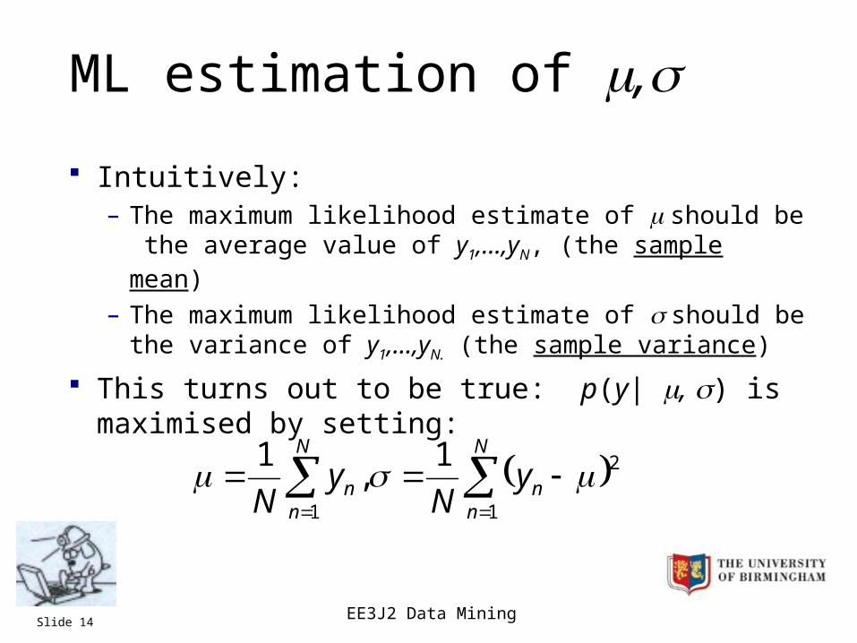
ML estimation of ,
Intuitively:– The maximum likelihood estimate of should be the
average value of y1,…,yN, (the sample mean)
– The maximum likelihood estimate of should be the variance of y1,…,yN. (the sample variance)
This turns out to be true: p(y| , ) is maximised by setting:
N
n
N
nnn y
Ny
N 1 1
21,
1
EE3J2 Data MiningSlide 15
Multi-modal distributions
In practice the distributions of many naturally occurring phenomena do not follow the simple bell-shaped Gaussian curve
For example, if the data arises from several difference sources, there may be several distinct peaks (e.g. distribution of heights of adults)
These peaks are the modes of the distribution and the distribution is called multi-modal
EE3J2 Data MiningSlide 16
Gaussian Mixture PDFs
Gaussian Mixture PDFs, or Gaussian Mixture Models (GMMs) are commonly used to model multi-modal, or other non-Gaussian distributions.
A GMM is just a weighted average of several Gaussian PDFs, called the component PDFs
For example, if p1 and p2 are Gaussiam PDFs, then
p(y) = w1p1(y) + w2p2(y)
defines a 2 component Gaussian mixture PDF
EE3J2 Data MiningSlide 17
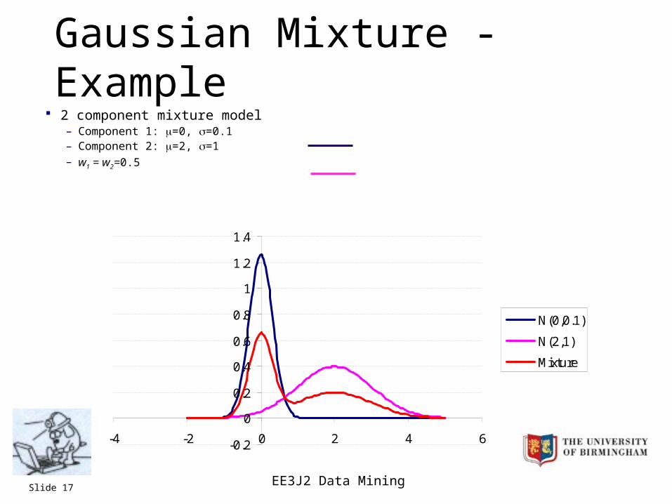
Gaussian Mixture - Example 2 component mixture model
– Component 1: =0, =0.1– Component 2: =2, =1– w1 = w2=0.5
-0.2
0
0.2
0.4
0.6
0.8
1
1.2
1.4
-4 -2 0 2 4 6
N(0,0.1)
N(2,1)
Mixture
EE3J2 Data MiningSlide 18
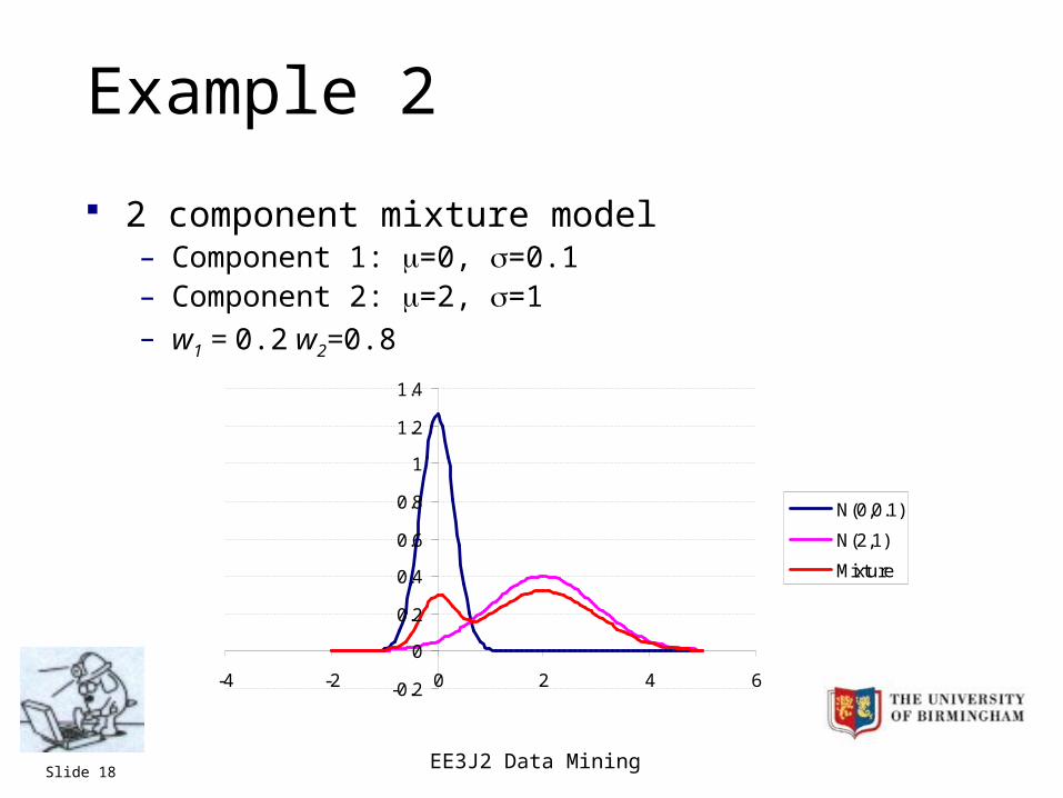
Example 2
2 component mixture model– Component 1: =0, =0.1– Component 2: =2, =1– w1 = 0.2 w2=0.8
-0.2
0
0.2
0.4
0.6
0.8
1
1.2
1.4
-4 -2 0 2 4 6
N(0,0.1)
N(2,1)
Mixture
EE3J2 Data MiningSlide 19
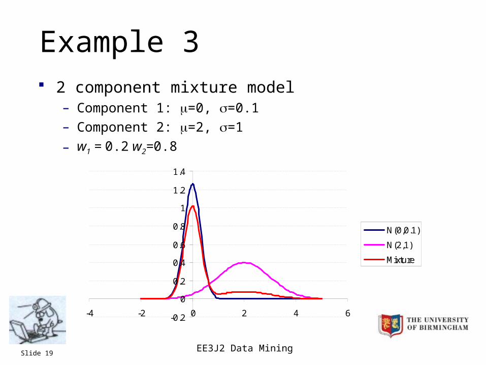
Example 3 2 component mixture model
– Component 1: =0, =0.1
– Component 2: =2, =1
– w1 = 0.2 w2=0.8
-0.2
0
0.2
0.4
0.6
0.8
1
1.2
1.4
-4 -2 0 2 4 6
N(0,0.1)
N(2,1)
Mixture
EE3J2 Data MiningSlide 20
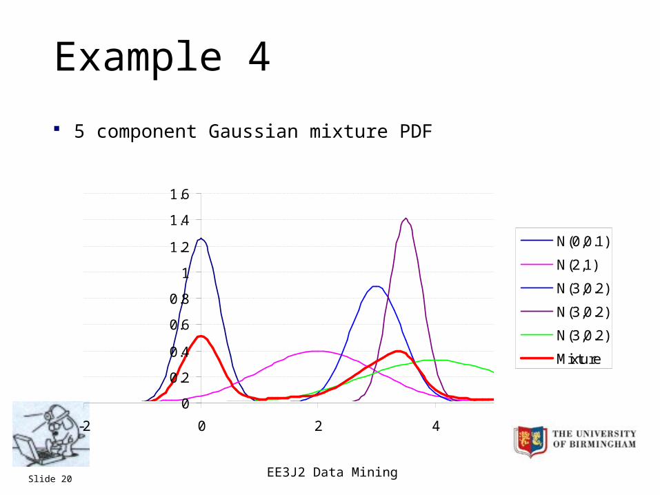
Example 4
5 component Gaussian mixture PDF
0
0.2
0.4
0.6
0.8
1
1.2
1.4
1.6
-2 0 2 4
N(0,0.1)
N(2,1)
N(3,0.2)
N(3,0.2)
N(3,0.2)
Mixture
EE3J2 Data MiningSlide 21
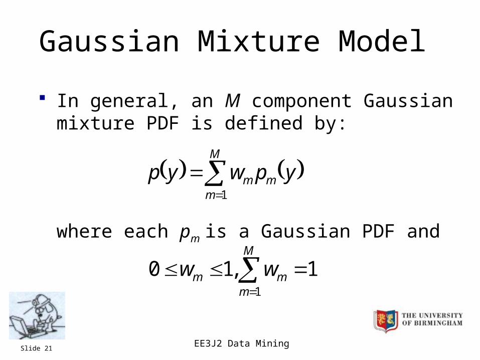
Gaussian Mixture Model
In general, an M component Gaussian mixture PDF is defined by:
where each pm is a Gaussian PDF and
M
mmm ypwyp
1
M
mmm ww
1
1,10
EE3J2 Data MiningSlide 22
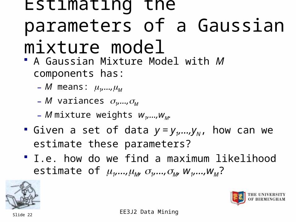
Estimating the parameters of a Gaussian mixture model A Gaussian Mixture Model with M components has:
– M means: 1,…,M
– M variances 1,…,M
– M mixture weights w1,…,wM.
Given a set of data y = y1,…,yN, how can we estimate these parameters?
I.e. how do we find a maximum likelihood estimate of 1,…,M, 1,…,M, w1,…,wM?
EE3J2 Data MiningSlide 23
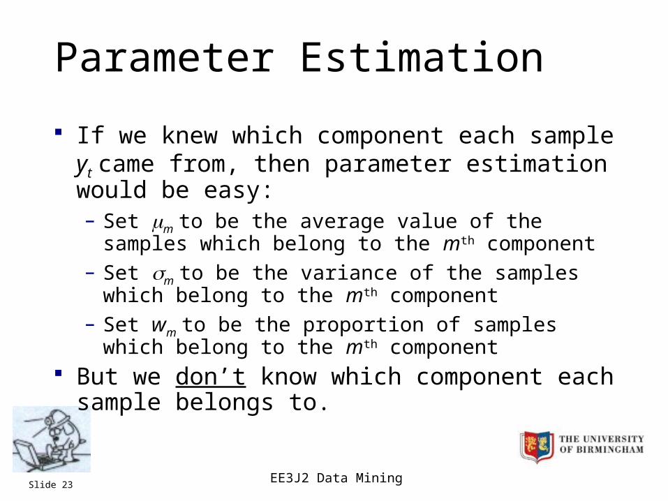
Parameter Estimation
If we knew which component each sample yt came from, then parameter estimation would be easy:– Set m to be the average value of the samples which
belong to the mth component– Set m to be the variance of the samples which belong to
the mth component– Set wm to be the proportion of samples which belong to
the mth component But we don’t know which component each sample
belongs to.
EE3J2 Data MiningSlide 24
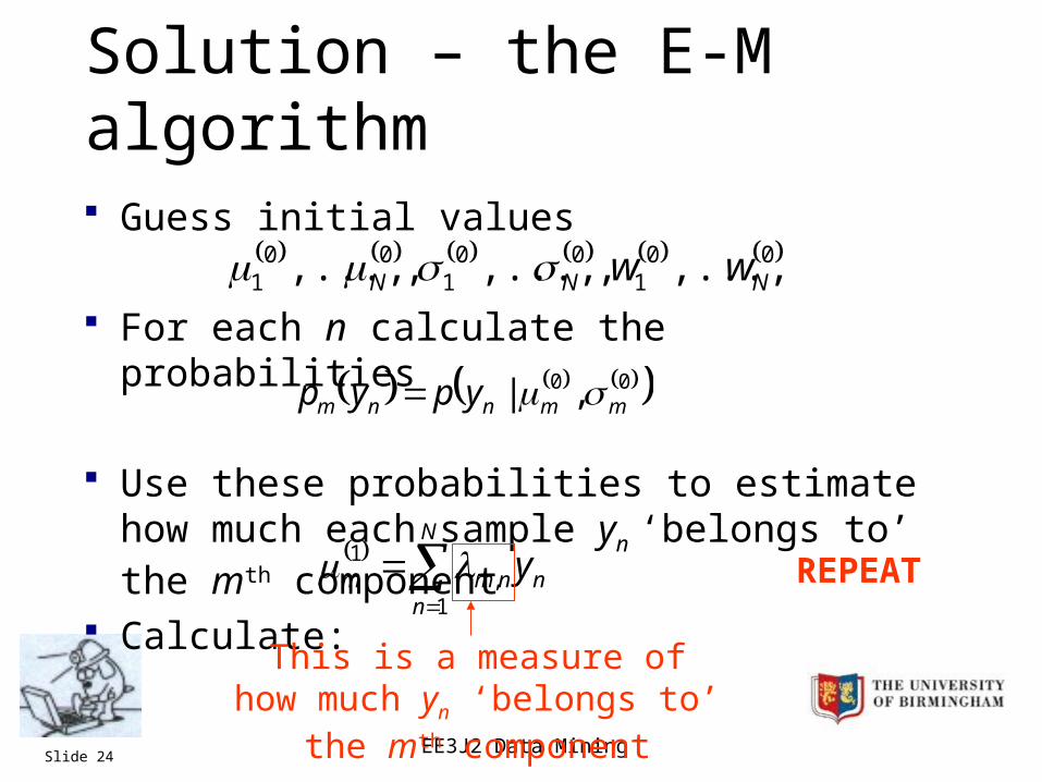
Solution – the E-M algorithm
Guess initial values
For each n calculate the probabilities
Use these probabilities to estimate how much each sample yn ‘belongs to’ the mth component
Calculate:
001
001
001 ,...,,,...,,,..., NNN ww
00 ,| mmnnm ypyp
N
nnnmm y
1,
1
This is a measure of how much yn ‘belongs to’ the mth component
REPEAT
EE3J2 Data MiningSlide 25
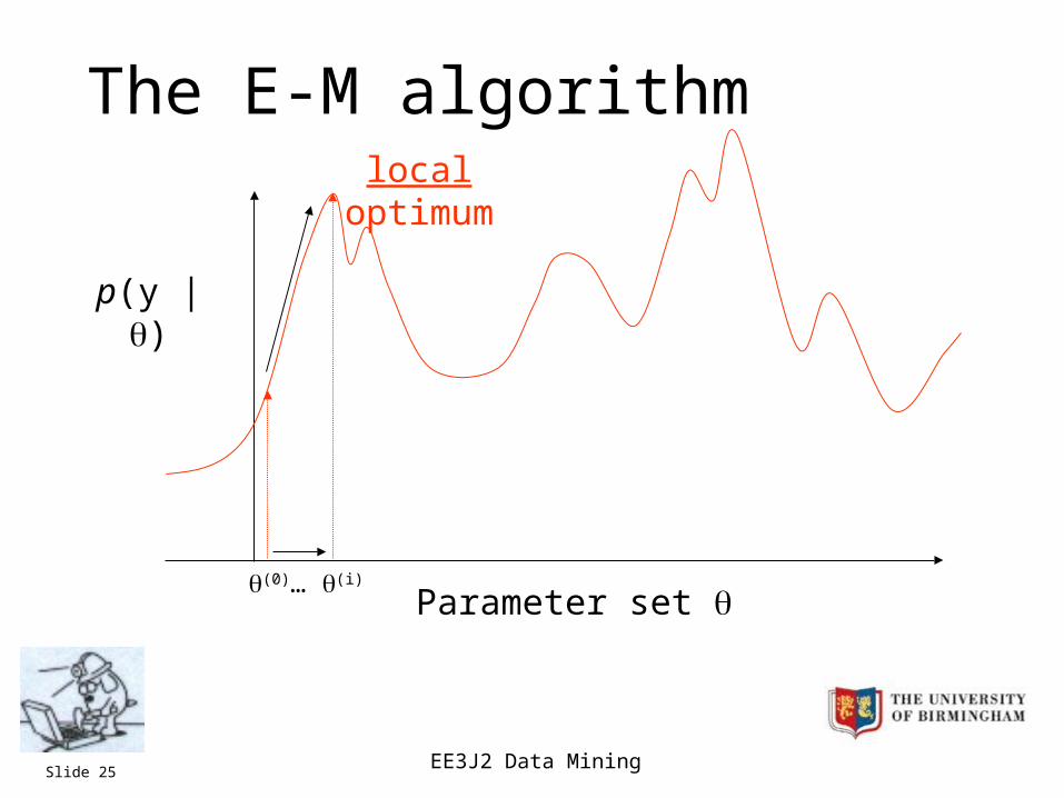
The E-M algorithm
Parameter set
p(y | )
(0)… (i)
local optimum
EE3J2 Data MiningSlide 26
Multivariate Gaussian PDFs
All PDFs so far have been 1-dimensional They take scalar values But most real data will be represented as D-
dimensional vectors The vector equivalent of a Gaussian PDF is called a
multivariate Gaussian PDF
EE3J2 Data MiningSlide 27
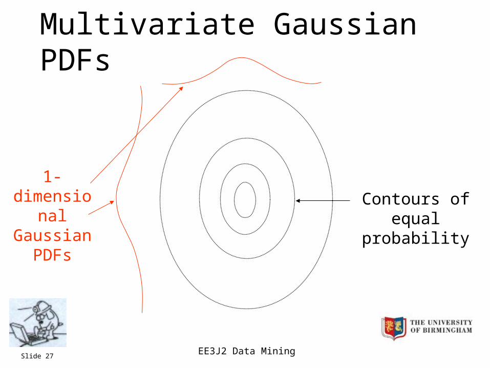
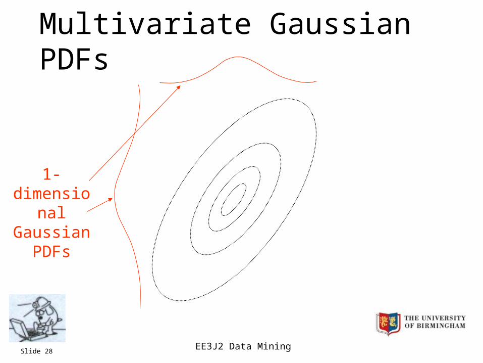
Multivariate Gaussian PDFs
Contours of equal probability
1-dimensional
Gaussian PDFs
EE3J2 Data MiningSlide 28
Multivariate Gaussian PDFs
1-dimensional
Gaussian PDFs
EE3J2 Data MiningSlide 29
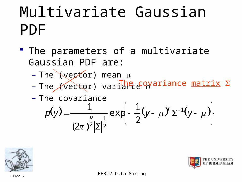
Multivariate Gaussian PDF
The parameters of a multivariate Gaussian PDF are:– The (vector) mean – The (vector) variance – The covariance The covariance matrix
yyyp T
p1
2
12
2
1exp
)2(
1
EE3J2 Data MiningSlide 30
Multivariate Gaussian PDFs
Multivariate Gaussian PDFs are commonly used in pattern processing and data mining
Vector data is often not unimodal, so we use mixtures of multivariate Gaussian PDFs
The E-M algorithm works for multivariate Gaussian mixture PDFs
EE3J2 Data MiningSlide 31
Summary
Basic statistical modelling Probability distributions Probability density function Gaussian PDFs Gaussian mixture PDFs and the E-M algorithm Multivariate Gaussian PDFs
EE3J2 Data MiningSlide 32
Summary
Related Documents