slac-r-680

SLAC-R-680

STUDY OF B ANTI-B PRODUCTION IN E+ E- ANNIHILATION AT S**(1/2) = 29-GEV WITH THE AID OF NEURAL NETWORKS *

David Joel Lambert

Stanford Linear Accelerator Center Stanford University Stanford, CA 94309

SLAC-Report-680

Prepared for the Department of Energy under contract number DE-AC03-76SF005 15

Printed in the United States of America. Available from the National Technical Information Service, U.S. Department of Commerce, 5285 Port Royal Road, Springfield, VA 22161.

~~

Ph.D. thesis, University of California and Lawrence Berkeley Laboratory, Berkeley, CA 94720.

LBL-36353 UC-414

Study of bg Production in e+e- Annihilation at 6= 29 GeV with the Aid of Neural Networks

David Joel Lambert Ph.D. Thesis

Department of Physics University of California

and

Physics Division Lawrence Berkeley Laboratory

University of California Berkeley, CA 94720

November 1994

This work was supported by the Director, Office of Energy Research, Office of High Energy and Nuclear Physics, Division of High Energy Physics, of the U.S. Department of Energy under Contract No. DE-AC03- 76SF00098.

1

LBL-36353 UC-414

Study of bb Production in e+e- Annihilation at .Js = 29 GeV with the Aid of Neural

Networks

David Joel Lambert PhD Thesis

Department of Physics University of California, Berkeley

and Lawrence Berkeley Laboratory

University of California, Berkeley

November 15, 1994

Abstract

We present a measurement of a(b6)/a(qq) in the annihilation process e+e- --+ qq -+ hadrons at f i = 29 GeV. The analysis is based on 66 pb-' of data collected between 1984 and 1986 with the TPC/2y detector at PEP. To identify bottom events, we use a neural network with inputs that are computed from the 3-momenta of all of the observed charged hadrons in each event. We also present a study of bias in techniques for measuring inclusive T*, K*, and p/p production in the annihilation process e'e- b6 + hadrons at f i = 29 GeV, using a neural network to identify bottom-quark jets. In this study, charged particles are identified by a simultaneous measurement of momentum and ionization energy loss (dE/dz).

This work is supported by the United States Department of Energy under Contract DE-AC03-76SF00098.

1

.. 11

Acknowledgements

I consider it a privilege to have participated, with so many gifted people, in a scientific endeavor that aimed to better understand the fundamental workings of the universe. It was a tragedy for all involved that the experiment had to be terminated before we could reap the rewards of the many person-years of labor spent readying it for its high-luminosity running. We can now only dream of what we might have accomplished with such a powerful detector.

I am indebted to many people on the TPC/Two-Gamma experiment who gladly aided me in my quest to do good physics and to earn a doctorate. Most of all, I am indebted to Michael Ronan, who patiently guided me through my entire career as a graduate student on the TPC/Two-Gamma experiment. He provided me with many good ideas that helped make this analysis what it is (e.g. using a neural network), and it was he who encouraged me during my low points. I am very grateful to Ron Ross, who, with Michael Ronan, served as my dissertation advisor; he asked many good questions, always reminded me of the big picture, and always treated me warmly.

I am also grateful to Gerry Lynch, who taught me much of what I now know of statistics, dE/dz, data processing, and optimization, and who always welcomed my questions. Gerry and Mike also did the work of including the CLEO Monte Carlo into the standard TPC/Two-Gamma Monte Carlo. Phillipe Eberhard came up with the idea of requiring f$ED = fz:? in Section 7.6, he is chiefly responsible for creating the binned maximum Likelihood fit method described in Section 7.3.2, and his perceptive responses to my analysis progress reports were invaluable. I had many good discussions with Jeremy Lys and Hiro Yamamoto. Lynn Stevenson, Marjorie Shapiro, Orin Dahl, A1 Clark, Werner Koellner, Jim Dodge, John Waters, and Tim Edberg all provided valuable assistance. Shigeki Misawa provided me with much information that was valuable for my job-hunt.

Allen Nicol joined the experiment about when I did. I treasured his compan- ionship in the trenches. I shall never forget the gnarly rubber band fights with Brent Corbin. I thank the DO collaboration at LBL for allowing me access to their workstations. I am grateful to Allen, Tim Edberg, Glen Cowan, and Jack East- man for letting me ‘borrow’ their figures. I wish to thank SeLig Kaplan, Marjorie Shapiro, Ron Ross, and Mike Ronan, the members of the committee who read this

... lll

dissertation. I am forever indebted to David for his personal guidance. I have been deeply

enriched by the friendship of Doyle, Jan, Val, Joyce, and Robin, and the love and friendship of Karen, Tina, and Tracy. Doyle taught me the true meaning of friendship: he typed in a large portion of this dissertation over many hours when I was unable to type because of tendonitis. My parents are world class parents, even when they asked for the latest estimate of my graduation date. AGSE and HAI made life even more interesting.

This dissertation is dedicated to the wonderful people and land of the San Francisco Bay Area.

iv

Contents

Acknowledgements ii

1 Overview 1

2 The Theory of Hadron Production in e+e- Annihilation 3

2.1 Quarks and Their Properties . . . . . . . . . . . . . . . . . . . . . . 3

2.2 Production of qq in e+e- Annihilation . . . . . . . . . . . . . . . . 5

2.3 QCD in e+e- Annihilation . . . . . . . . . . . . . . . . . . . . . . . 7

2.3.1 Fixed Order Computations in QCD . . . . . . . . . . . . . . 7

2.3.2 The Leading Logarithm Approximation of QCD . . . . . . . 8

2.3.3 Where Perturbative QCD Fails . . . . . . . . . . . . . . . . 8

2.4 Models of Hadronization . . . . . . . . . . . . . . . . . . . . . . . . 9

2.4.1 Independent Ragmentation . . . . . . . . . . . . . . . . . . 9

2.4.2 String Fragmentation . . . . . . . . . . . . . . . . . . . . . . 12

2.4.3 Cluster Fragmentation . . . . . . . . . . . . . . . . . . . . . 17

2.5 The Properties of Heavy Quark Events . . . . . . . . . . . . . . . . 21

2.6 Previously Used Heavy Quark Event Tags . . . . . . . . . . . . . . 22

2.7 Corrections to a(bE)/a(qq) . . . . . . . . . . . . . . . . . . . . . . . 24

2.4.4 The Peterson Fragmentation Function . . . . . . . . . . . . 19

3 The TPC/Two-Gamma Experiment 27

3.1 The TPC/Two-Gamma Detector . . . . . . . . . . . . . . . . . . . 27

3.2 The Time Projection Chamber . . . . . . . . . . . . . . . . . . . . . 32

3.3 Calibration of the TPC . . . . . . . . . . . . . . . . . . . . . . . . . 34

V

4 Particle Identification Using the TPC 35 4.1 The Measurement of Momentum . . . . . . . . . . . . . . . . . . . 35 4.2 The Theory of dE/dz Energy Loss . . . . . . . . . . . . . . . . . . 36 4.3 dE/dz Resolution Parameterization . . . . . . . . . . . . . . . . . . 39

5 Event Reconstruction. Selection. and Simulation 44 5.1 Event Reconstruction . . . . . . . . . . . . . . . . . . . . . . . . . . 44 5.2 Event Selection . . . . . . . . . . . . . . . . . . . . . . . . . . . . . 44 5.3 Event Simulation . . . . . . . . . . . . . . . . . . . . . . . . . . . . 47

5.3.1 The Event Simulation Software Package . . . . . . . . . . . 47 5.3.2 Tuning the Peterson Parameterization . . . . . . . . . . . . 48 5.3.3 Tuning the Jetset Event Shape Parameters . . . . . . . . . . 49

6 Feed-Forward Neural Networks 60 6.1 Neural Network Architecture . . . . . . . . . . . . . . . . . . . . . . 60 6.2 The Training of a Neural Network . . . . . . . . . . . . . . . . . . . 62 6.3 Measuring Network Performance . . . . . . . . . . . . . . . . . . . . 65 6.4 Previous Uses of Neural Networks in High Energy Physics . . . . . 67

6.4.1 Classification Using Neural Networks . . . . . . . . . . . . . 67 6.4.2 Fitting in a Neural Network Output . . . . . . . . . . . . . . 67

7 A Measurement of the Bottom Event Production Fraction 72 7.1 The Choice of Neural Network Inputs and Architecture . . . . . . . 72 7.2 Training the Event-Tagging Neural Network . . . . . . . . . . . . . 74 7.3 The Method for Fitting the Bottom Event Fraction . . . . . . . . . 80

7.3.1 The Extended Maximum Likelihood Method . . . . . . . . . 82 7.3.2 The Event Fraction Likelihood Function . . . . . . . . . . . 82

7.4 The Bottom Event Fraction . . . . . . . . . . . . . . . . . . . . . . 85 7.4.1 The Fit of the Bottom Event Fraction . . . . . . . . . . . . 85 7.4.2 Correcting for Backgrounds . . . . . . . . . . . . . . . . . . 85 7.4.3 Acceptance and Physics Corrections . . . . . . . . . . . . . . 88

7.5 The Evaluation of Systematic Errors . . . . . . . . . . . . . . . . . 89 7.5.1 91

7.5.2 Systematic Errors due to the Detector Simulation . . . . . . 92 7.6 The Monte Carlo Bottom Event Fraction . . . . . . . . . . . . . . . 94

Systematic Errors in the Simulation of ese- -+ qq . . . . . .

vi

7.7 Discussion of the Results . . . . . . . . . . . . . . . . . . . . . . . . 99

7.7.1 How a( fQED) Depends Upon a(f2zy) . . . . . . . . . . . . 99 7.7.2 Comparison to LEP Measurements of I'(Zo-+ bb) . . . . . . 100

8 A Study of Bias in Techniques to Measure Charged Hadron Pro- duction in Bottom Quark Jets 103 8.1 Introduction . . . . . . . . . . . . . . . . . . . . . . . . . . . . . . . 104 8.2 Track and Event Selections . . . . . . . . . . . . . . . . . . . . . . . 104 8.3 The Jet-Tagging Neural Network . . . . . . . . . . . . . . . . . . . 105 8.4 Techniques for Measuring Charged Hadron Production in Bottom

Quark Jets . . . . . . . . . . . . . . . . . . . . . . . . . . . . . . . . 113 8.5 A Test for Bias in Measurements of Charged Hadron Production in

Bottom Quark Jets . . . . . . . . . . . . . . . . . . . . . . . . . . . 120 8.6 An Investigation of the Sources of Bias . . . . . . . . . . . . . . . . 121

8.6.1 Using Correlations Between Jets in Each Event to Measure Bias . . . . . . . . . . . . . . . . . . . . . . . . . . . . . . . 121

8.6.2 All Possible Sources of Correlations . . . . . . . . . . . . . . 126 8.6.3 Which Sources of Correlation Contribute . . . . . . . . . . . 127 8.6.4 The Relative Importance of the Sources of Correlation . . . 135 8.6.5 Comparing Monte Carlo Correlations to Experimental Data

Correlations . . . . . . . . . . . . . . . . . . . . . . . . . . . 141 8.7 Summary . . . . . . . . . . . . . . . . . . . . . . . . . . . . . . . . 143

9 Conclusions 145

AppendixA Remainder of the Proof of the Event Fraction Likeli- hood Function Optimization Method 147 A.1 The Case some but not all r n ; j = 0 . . . . . . . . . . . . . . . . . . 147

147 A . l . l The Subcase $ - 1 < - . . . . . . . . . . . . . . . . . . . A.1.2 The Subcase & 5 . 1 . . . . . . . . . . . . . . . . . . . . 148

A.2 The Case mij = 0 for all i . . . . . . . . . . . . . . . . . . . . . . . 148

1 aM'

Appendix B F for Any Number of Classes 149 B. l K Event Classes with Complete Separation . . . . . . . . . . . . . . 150 B.2 Computing the F's . . . . . . . . . . . . . . . . . . . . . . . . . . . 150

Bibliography 151

1

V i i

List of Tables

2.1 The properties of quarks . . . . . . . . . . . . . . . . . . . . . . . . . 4 2.2 Some hadrons containing heavy quarks . . . . . . . . . . . . . . . . . 6 2.3 Properties of jets of different flavors . . . . . . . . . . . . . . . . . . 22 2.4 Previous hadronization measurements for different quark flavors . . . 24

5.1 Tuned values of the Lund flavor parameters in Jetset 7.2. . . . . . . 48 5.2 ( z ~ ) b a n d ( Z E ) ~ . . . . . . . . . . . . . . . . . . . . . . . . . . . . . . 49 5.3 E&, and ec for Jetset 7.2. . . . . . . . . . . . . . . . . . . . . . . . . . 49 5.4 Variables used for tuning . . . . . . . . . . . . . . . . . . . . . . . . 51 5.5 Tune of the Lund parameters in Jetset 7.2. . . . . . . . . . . . . . . 56

7.1 The values of F for the 7 event-tagging network inputs . . . . . . . . 74

7.2 Tune of the Lund event shape parameters in Jetset 7.2. . . . . . . . 92 7.3 The systematic errors in the Monte Carlo . . . . . . . . . . . . . . . 93 7.4 fz:? for five different values of fMc . . . . . . . . . . . . . . . . . 95

The correlation matrix for the five values of fzzf . . . . . . . . . . .

Q E D

7.5 The best-fit parabola . . . . . . . . . . . . . . . . . . . . . . . . . . . 96 7.6 97

7.7 All measurements of the bottom event fraction using a neural network.101

8.1 8.2

8.3 8.4

8.5 8.6 8.7

8.8

The baseline for the investigation of the sources of correlation . . . . 128

Correlations due to ISR and gluon radiation . . . . . . . . . . . . . . 130 Correlations due to ISR and gluon radiation, axes "iterated" . . . . . 131 Correlations from event shape/direction measurements . . . . . . . . 133

Correlations from fragmentation physics . . . . . . . . . . . . . . . . 129

Correlations due to detector acceptance . . . . . . . . . . . . . . . . 134 Correlations from event selections . . . . . . . . . . . . . . . . . . . . 136

Correlations caused by interactions in the detector material . . . . . 137

1

... VUI

8.9 Correlations relative to “Baseline 2” . . . . . . . . . . . . . . . . . . 139 8.10 Correlations relative to “Baseline 3” . . . . . . . . . . . . . . . . . . 140

8.11 The effect of axis “iterating” on correlations . . . . . . . . . . . . . . 141 8.12 Correlations in the Jet-Tagging Network Inputs, for Monte Carlo

and for experimental data . . . . . . . . . . . . . . . . . . . . . . . . 142 8.13 Correlations in the Jet-Tagging Network Output, for Monte Carlo

and for experimental data . . . . . . . . . . . . . . . . . . . . . . . . 143

1

... vu1

8.9 Correlations relative to “Baseline 2”. . . . . . . . . . . . . . . . . . 139 8.10 Correlations relative to (‘Baseline 3”. . . . . . . . . . . . . . . . . . 140

8.11 The effect of axis “iterating” on correlations. . . . . . . . . . . . . . 141 8.12 Correlations in the Jet-Tagging Network Inputs, for Monte Carlo

and for experimental data. . . . . . . . . . . . . . . . . . . . . . . . 142 8.13 Correlations in the Jet-Tagging Network Output, for Monte Carlo

and for experimental data. . . . . . . e . . . . . . . . . . . . . . 143

”. .

ix

List of Figures

2.1 2.2

2.3 2.4

The Standard Model fermions . . . . . . . . . . . . . . . . . . . . . . The independent fragmentation process . . . . . . . . . . . . . . . . Flux lines for an electric dipole and for color dipole . . . . . . . . . . The yo-yo model of a meson in string fragmentation . . . . . . . . .

2.5 String fragmentation . . . . . . . . . . . . . . . . . . . . . . . . . . . 2.6 Cluster fragmentation . . . . . . . . . . . . . . . . . . . . . . . . . . 2.7 The Peterson fragmentation function . . . . . . . . . . . . . . . . . .

3.1 3.2 3.3 3.4 3.5 A TPC sector . . . . . . . . . . . . . . . . . . . . . . . . . . . . . . . 3.6

The PEP storage ring . . . . . . . . . . . . . . . . . . . . . . . . . . The TPC/2y detector, 3-D representation . . . . . . . . . . . . . . . The TPC/2y detector. side view . . . . . . . . . . . . . . . . . . . . The TPC/2y detector. end view . . . . . . . . . . . . . . . . . . . .

The Time Projection Chamber wires . . . . . . . . . . . . . . . . . .

4.1 4.2 4.3 4.4

4.5

Distribution of dE/da: energy loss . . . . . . . . . . . . . . . . . . . Dependence of (dE/dz) on r ] = Py . . . . . . . . . . . . . . . . . . . dE/da: as a function of log(p) . . . . . . . . . . . . . . . . . . . . . .

for pions . . . . . . . . . . . . . . . . . . . . . . . . . . . . . . . . . Number of pions as a function of ( R - l ) / a ( N . A) . . . . . . . . . . . .

Scatterplot of N , the number of wire hits, as a function of I sin AI

5.1 Discrepancy between Monte Carlo and Experiment 14-18 data without and with the T-27 selection for the multiplicity. thrust minor.

Comparison of experimental data to tuned Monte Carlo in the tun-

Comparison of experimental data to tuned Monte Carlo in the tun-

and thrust major . . . . . . . . . . . . . . . . . . . . . . . . . . . . .

ing variables . . . . . . . . . . . . . . . . . . . . . . . . . . . . . . .

ing variables . . . . . . . . . . . . . . . . . . . . . . . . . . . . . . .

5.2

5.3

4 10 13 14 16 18 20

28 29 30 31 33 33

37 38 40

41 43

55

56

57

X

5.4 Comparison of experimental data to tuned Monte Carlo in the tun- ingvariables . . . . . . . . . . . . . . . . . . . . . . . . . . . . . . . 58

6.1 A one hidden layer neural network . . . . . . . . . . . . . . . . . . . 61 6.2 The DO electron-hadron calorimeter neural network . . . . . . . . . . 68

6.3 L3 fit of I’(bb) with a neural network . . . . . . . . . . . . . . . . . . 69 6.4 DELPHI neural network output distributions . . . . . . . . . . . . . 71

7.1

7.2 7.3

Event-Tagging Neural Network Inputs 1.4 . . . . . . . . . . . . . . . Event-Tagging Neural Network Inputs 5.7 . . . . . . . . . . . . . . . F as a function of the number of hidden nodes for the Event-Tagging Neural Network . . . . . . . . . . . . . . . . . . . . . . . . . . . . . . F as a function of the number of patterns per Event-Tagging Net- work parameter . . . . . . . . . . . . . . . . . . . . . . . . . . . . . . F as a function of epoch number for the Event-Tagging Neural Net- work . . . . . . . . . . . . . . . . . . . . . . . . . . . . . . . . . . . .

7.6 The Experiment 14-18 event-tagging neural network output distribution . . . . . . . . . . . . . . . . . . . . . . . . . . . . . . . . . . .

7.7 The Monte Carlo event-tagging neural network output distributions . 7.8 The fit of the bottom event fraction . . . . . . . . . . . . . . . . . . 7.9 Bottom event efficiency and purity as a function of neural network

output . . . . . . . . . . . . . . . . . . . . . . . . . . . . . . . . . . . 7.10 Measured b-event fraction as a function of Monte Carlo b-event

fraction . . . . . . . . . . . . . . . . . . . . . . . . . . . . . . . . . . 7.11 The difference between the measured and Monte Carlo b-event frac-

tions . . . . . . . . . . . . . . . . . . . . . . . . . . . . . . . . . . . . 7.12 Geometrical picture of how the error is mapdied . . . . . . . . . . .

7.4

7.5

75

76

77

78

79

80 81 86

87

96

98

100

8.1 8.2 8.3

8.4 8.5 8.6 8.7

8.8

The uniterated coordinate system . . . . . . . . . . . . . . . . . . . . 107 The iterated coordinate system . . . . . . . . . . . . . . . . . . . . . 107

Jet-Tagging Neural Network inputs 1. 4. 7. and 10 . . . . . . . . . . 110 Jet-Tagging Neural Network inputs 2. 5 . 8. and 11 . . . . . . . . . . 111 Jet-Tagging Neural Network inputs 13. 14. and 15 . . . . . . . . . . 112

Network . . . . . . . . . . . . . . . . . . . . . . . . . . . . . . . . . . 113

Jet-Tagging Neural Network inputs 3. 6. 9. and 12 . . . . . . . . . . 109

F as a function of the number of hidden nodes for the Jet Neural

F as a function of epoch number for the Jet-Tagging Neural Network . 114

xi

8.9 Jet-Tagging Neural Network output distribution for Experiments

8.10 Jet-Tagging Neural Network output distributions for Monte Carlo. . 116 8.11 The fit of the bottom jet fraction. . . . . . . . . . . . . . . . . . . . 117

8.12 Bottom jet efficiency and purity as a function of neural network output. . . . . . . . . . . . . . . . . . . . . . . . . . . . . . . . . . . 118

8.13 The bin-by-bin confidence levels for the scaled pion cross-section to be independent of the network output. . . . . . . . . . . . . . . . . 122

8.14 The bin-by-bin confidence levels for the scaled kaon cross-section to be independent of the network output.

8.15 The bin-by-bin confidence levels for the scaled proton cross-section to be independent of the network output. . . . . . . . . . . . . . . . 124

8.16 The sum of three independent distributions is not independent. . . 125

14-18. . . . . . . . . , . . . . . . . . . . . . . . . . . . . . . . . . . 115

. . . . . . . . . . . . . . . . 123

.. .

1

Chapter 1

Overview

In the Standard Model of elementary particle physics, fermionic quarks and leptons interact through the exchange of force-mediating bosons.

1. Photons mediate the electromagnetic interaction, which is described by Quantum Electrodynamics (QED).

2. The W* and the Zo, which are unified with the photon in the Weinberg- Salam model, mediate the weak interaction responsible for radioactive decay.

3. Gluons mediate the strong (color) interaction that binds quarks into hadrons. The theory of the color force is Quantum Chromodynamics, abbre- viated QCD.

The Standard Model is very successful: it has survived many tests, made many successful predictions, and does not conflict with any experimental observations.

We measure the ratio n(bE)/u(qq) in this dissertation, since this ratio is a fundamental prediction of the Standard Model that has never been directly measured near 29 GeV. The analysis is based on 66 pb-l of data collected between 1984 and 1986 with the TPC/2y detector at PEP.

Past measurements of the propkrties of bottom events used standard methods for identifying, or tagging, bottom events. These methods collected fairly high- purity bottom event samples, but with low efficiency: most bottom events are excluded from the bottom sample. We take a new approach in order to use the data more efficiently: we use a neural network with inputs that are computed from the 3-momenta of all of the observed charged hadrons in each event.

One of the few outstanding problems of the Standard Model is that, as of now, we have neither the theoretical nor the computational ability to make quantitative predictions with QCD for processes with momentum-transfers of the order of 1

2

GeV/c or less. One of these low-momentum-transfer processes is hadronization, in which colored quarks and gluons are confined within colorless hadrons.

To point the way towards improving our understanding of hadronization, we also present a study of bias in techniques for measuring inclusive T*, K*, and p/ij production in the annihilation process e+e- --+ bb + hadrons at f i = 29 GeV, using a neural network to identify the contribution of bottom-quark jets.

Chapter 2 contains a review of the theory of hadronization in e+e- annihilation, a discussion of the previous measurements of hadronization for events produced by different kinds of quarks, and a review of the theory of e+e- annihilation that we use to determine the theoretical value of the ratio a(bb)/a(q$ to compare to our measurement of this ratio. In Chapter 3, we provide a brief description of that part of the TPC/Two-Gamma experiment which is relevant to this measurement, and in Chapter 4, we describe particle identification using the TPC. In Chapter 5, we describe the processing, selection, and simulation of the e+e- --+ hadrons data. Chapter 6 contains our description of the use of neural networks. In Chapter 7, we describe and discuss the measurement of the ratio a(bb)/u(qq). In Chapter 8, we present a study of bias in techniques for measuring inclusive T*, K*, and p/p production in bottom jets. In Chapter 9, we summarize the results.

3

Chapter 2

The Theory of Hadron Production in &e- Annihilation

In this chapter, we review the present understanding of the process ese- + qij -+ hadrons. We also discuss the implications of this understanding for the ratio a(bb)/a(qij) and for the differences between bottom and non-bottom events. Fi- nally, we review previous measurements of hadronization for events produced by different kinds of quarks.

2.1 Quarks and Their Properties

In order to understand the process ese- + qi j + hadrons, we must first be familiar with some of the properties of quarks.

Matter is known to be composed of two classes of spin-1/2 particles: leptons and quarks. The distinction between these classes of particles is that while the quarks carry color charge and feel the strong force, the leptons do not. In the Standard Model, the particles are arranged into doublets [I] as shown in Figure 2.1. As far as we can tell, quarks and leptons are fundamental point particles with no sub-structure [2]. ,

Some of the properties of the quarks are listed in Table 2.1. Quarks have never been observed in isolation and are apparently always confined within hadrons [4], so the masses of the quarks are not precisely known. The up, down, and strange quarks are referred to collectively as the light quarks, while the others are referred to collectively as the heavy quarks. The top quark is too heavy to be pair-produced at the center-of-mass energy of this experiment, 29 GeV, so when we refer to heavy quarks in this dissertation, we mean the charm and bottom quarks.

While it is conventional to refer to quarks only by their type, or flavor, each

4

Leptons Quarks

Figure 2.1: The Standard Model fermions (From [3]).

strange charm bottom

abbreviation electric charge I mass -113 e +2/3 e -113 e +2/3 e -1/3 e +2/3 e

9.9 k 1.1 MeV/? [5] 5.6 3.1 1.1 MeV/? [5] 199 f 33 MeV/c2 [5 ]

11.35 f 0.05 GeV/c2 [5] -5 GeV/c2 [6]

174 f 102;; GeV/c2 [7]

Table 2.1: The properties of quarks.

5

quark listed in Table 2.1 actually represents three different quarks which are identical except that each has a different color (red, green, or blue). Likewise, antiquarks have one of 3 anticolors (anti-red, anti-green, or anti-blue), and gluons one of the 8 color-octet combinations of a color and an anticolor. Quantum Chromodynamics (QCD) is the theory of the color (or strong) force [8], in which gluons mediate the interaction between particles that possess a color charge. It is widely believed, but not proven, that the confinement of quarks and gluons within colorless hadrons is a property of QCD.

As far as we know, there are two ways of forming color-neutral hadrons from quarks. Mesons are made of a quark and an antiquark of the same color, such as red and anti-red. Examples of mesons are the rITS (charged pion), with quark content d a n d mass 139.6 MeV/c2, and the KS (charged kaon), with quark content us and mass 493.7 MeV/c2. Baryons are a color-singlet combination of 3 quarks, each of which has a different color. The proton, with quark content uud and mass 938.3 MeV/c2, is a baryon. Table 2.2 lists some of the most commonly produced hadrons containing heavy quarks.

2.2 Production of qq in &e- Annihilation

In the first step in the process e'e- --+ qtj + hadrons, an electron and a positron annihilate into a virtual photon, which couples into a final state consisting of a quark and its antiquark. Quarks are fundamental spin-l/2 fermions, therefore the first approximation to the cross-section for e+e- --f qq, for a quark Q with electric charge Qqe, has the usual cross-section for massless fermions in Quantum Electro- dynamics (QED), the quantum theory of the electromagnetic force mediated by the photon [12]. This cross-section is

da CY2

dR 4s --- - [I +cos2e] Q; ,

[13], where s is the square of the center-of-mass energy of the e+e- system and a = e2/hc 21 1/137 is the dimensionless coupling strength of QED.

In this approximation, we compute

a(b6) = 3 - 4ncu2 ( i)2 = 0.0344 nb,

a(qq) = 3 - 4na2 [3 (i)' + 2 (:)2] = 0.3787 nb,

3s

3s

6

name D+ DO w D*+ D*O Df+ A,+ E,++ E: E: z+ -C

=O -C

BO B-

quark content C d

Ci i

CS

C a

C i i

CS

cdu cuu cdu cdd

csd ba bii bs ba bii bS

bdu

csu

spin mass ( GeV/c2) 1.869 1.865 1.969 2.010 2.007 2.110 2.285 2.453 2.453 2.453 2.466 2.473 5.279 5.279 5.375 5.325 5.325 5.422 5.64

Table 2.2: Some hadrons containing heavy quarks [9, 10, 111.

7

and cT(b6)/a(qq) = 1/11 M 0.0909 .

The overall factor of 3 in the cross-sections comes from the fact that each quark comes in 3 colors.

This is the lowest order approximation for the cross-sections. A discussion of higher-order effects in the calculation of these cross-sections is given in Section 2.7.

2.3 QCD in e+e- Annihilation

The quark and antiquark produced in e+e- annihilation, being colored objects, can radiate gluons, just as electric charges radiate photons. In QCD, quarks and gluons interact with a strength parameterized by a dimensionless coupling constant as(m) that is a function of Q2 = -q2 , where qp is the gluon 4-momentum. a, is said to mn with m. The leading logarithm approximation to this dependence is

127r a s (e) = ( 33 - 2 N f ) ln(Q2/R2) '

where N f is the number of quark flavors with mass less than m, and A is an experimentally measured constant' [MI. As decreases, a, (m) increases: a,(91 GeV) = .115 f .008 [15] and a,(34 GeV) = -14 Z!= .02 [16]. When is in the neighborhood of 1 GeV/c, a,(m) becomes of order 1. As long as a,(m) is much less than 1, perturbation theory can be used to calculate cross-sections.

We now review the two approaches to perturbative QCD calculations: fixed order, and the leading logarithm approximation.

2.3.1 Fixed Order Computations in QCD

These computations are for final states composed of a small, definite number of partons (a parton is a quark, an antiquark, or a gluon). An example of a fixed order perturbative computation is the total cross-section for e+e- annihilation into a maximum of 5 partons at center-of-mass energy f i . This computation shows that

'As f l decreases, so does N f , but aYd(@) is a continuous function of @, so each and all the A(Nf)ls are related by range of constant N f actually has its own constant

Equation 2.5 and the continuity of as(@).

8

for center-of-mass energy well above the b6 threshold and well below the Zo mass [17,18]. The 2' and the W* are the mediators of the weak force, which is described by the Weinberg-Salam model [ 191.

Another example of a fixed order perturbative computation is the differential cross-section for e+e- annihilation into a quark with a fraction xq = Eq/Eb,am of the total energy, an antiquark with a fraction xcQ = Eq/Ebeam of the total energy, and a gluon with a fraction xg = E,/&,, of the total energy [20]. The cross- section is

do 2a,(fi) xi + z; = a(e+e- + QQ)

dxqdxq 3n (1 - x q ) ( l -xq) *

This cross-section diverges for zero-energy gluons (xq = 1 and xcQ = l), for gluons colinear with the quark (2, = l), and for gluons colinear with the antiquark ( xg = 1). These divergences (poles) cancel with the divergences in diagrams where a gluon is emitted and reabsorbed by the same quark or antiquark.

2.3.2 The Leading Logarithm Approximation of QCD

The other approach to perturbative QCD is leading logarithm QCD. This approach sums up, to all orders, the most divergent processes at each order in perturbation theory. The divergences are the colinear singularities of the type found in Equa- tion 2.7.

Leading logarithm QCD allows us to model the perturbative evolution of an event as a series of the independent parton branchings q -+ qg , g + qij , and g 4 g g , with the probability of each branching given by one of the Altarelli-Parisi splitting functions [21]. The partons produced in each branching have lower virtuality than the original parton; the branching is stopped when the parton masses approach the energy scale Qo where perturbation theory fails. The entire branching process, illustrated in Figure 2.6a, is called a parton shower.

2.3.3 Where Perturbative QCD Fails

As f l decreases during the evolution of a hadronic event, a,(J&'i) increases ' until it becomes of order 1, at about 1 GeV/c. At this energy scale, perturbation theory fails. In this energy region, where confinement and hadronization occur, we must resort to other means for calculating amplitudes and cross-sections for hadron production.

Lattice computations of QCD are first-principles computations of QCD, but require an enormous amount of computation, so only now are we beginning to obtain useful results on the simplest of lattice calculations [22, 231. Detailed lattice QCD results on hadronization are still years away because of their complexity. As

9

of yet, there are no other methods for computing from first-principles QCD at low momentum transfer. Instead, we resort to phenomenological models of the hadronization process.

2.4 Models of Hadronization

There are a number of models of hadronization. Their Monte Carlo implementa- tions all start with the production of a set of partons, either by fixed order QCD or by a parton shower. The hadronization model then transforms the parton configuration into a set of hadrons. Finally, in the Monte Carlo implementation, those hadrons with relatively short lifetimes are decayed, producing a set of particles that live long enough to travel an observable distance. This set of particles is then compared to experimental data.

In this analysis, hadronization models are used to compute acceptances, test the analysis method of Chapter 8 for bias (Sections 8.6 and 8.5), and train the neural networks we use to distinguish bottom events from non-bottom events (Section 7.1) and 8.3).

The hadronization models we describe in this section have Monte Carlo im- plementations that we can use for all of these purposes. These models can be grouped into three classes: independent fragmentation, string fragmentation, and cluster fragmentation. We then discuss the Peterson fragmentation function that can be used in those models with a fragmentation function: independent and string fragmentation.

2.4.1 Independent Fragmentation

Historically, one of the first fragmentation models was the independent fragmentation model of Feynman and Field [24]. In this model, the original quark and antiquark each transform into a jet of hadrons, independently of each other.

Figure 2.2 illustrates the creation of a jet by independent fragmentation from a quark QO created in the process e+e- + q&. First, a quark pair ql& is created from the vacuum. ij1 and qo combine to form a meson, leaving behind q l , which has less energy than qo did. Then another pair q 2 i j 2 is created, and q1 and & bind together to form another meson, leaving behind q2 with still less energy. This process repeats itself until the remaining quark has too little energy to form a meson. The same kind of iterative process produces a second jet from qo.

It is assumed that the quarks and antiquarks created from the vacuum each have a transverse momentum that is distributed as a Gaussian with an experimentally determined width my. The total transverse momentum of each created pair is zero. Another experimentally measured parameter T determines the fraction of

t

10

Figure 2.2: The independent fragmentation process into mesons for a jet initiated by the quark qo. ‘h(qn&)’ is a meson with quark content qnQn (Based on 1251).

11

mesons that are vector, the remainder being pseudoscalar. A third adjustable parameter, P ( s ) / P ( u ) , determines the probability that the created qq pairs are ss, the remaining pairs being half ue and half dd.

Another feature of this model is a fragmentation function f (z) . It is the probability density, at each step in the fragmentation chain, that a fraction z of the momentum of quark qi goes into the meson formed by it and iji+l. The remaining momentum goes into qi+l. Feynman and Field chose

f (z ) = 1 - CL - 3 a ( l - z ) ~ ,

where a is determined from experiment.

Some of the hadrons created in this cascade (called primary hadrons) are un- stable and are decayed by the Monte Carlo implementation of the Feynman-Field model. The order in which these primary hadrons are created is called the rank the first primary hadron has rank 1, the second one has rank 2, etc.

The original Feynman-Field model did not include baryon production and gluon jets. Meyer [26] proposed an extension of the model in which occasionally two quark-antiquark pairs, rather than one, are created from the vacuum with probability P(qq) /P(q) . The qq then combines with the adjacent quark, and the @ combines with the adjacent antiquark, forming a baryon-antibaryon pair.

Hoyer [27] and Ali 1281 introduced gluon jets, which split into uG, dd; and S S pairs with equal probability. The quark and antiquark then fragment independently. Different variations on independent fragmentation divide the gluon momentum between the quark and antiquark differently. Massive quarks must be handled differently from light quarks; it was in this context that the Peterson function was invented (Section 2.4.4).

Even though independent fragmentation is basically a parameterization, rather than an attempt to model the fundamental dynamics of fragmentation, it is ef- fective in describing hadron production. This model simulates the jets in events independently of each other, so we use it in the studies in Section 8.6.

It is not the model of choice, however. It fails to reproduce the string effect [29, 30, 311. Also, it has a number of serious theoretical problems. There is no natural way of handling the last (anti)quark in each jet; some variations on independent fragmentation simply throw them away. Neither energy nor momentum is conserved, unless the jets are rescaled in E and/or p in an ad hoc manner [32]. Finally, since the properties of the cascade depend upon the initial (anti)quark momentum in the laboratory frame of reference, independent fragmentation is not Lorentz covariant.

12

2.4.2

Another , by Artru

String Fragmentation

more physical model of fragmentation is string fragmentation, proposed and Mennessier [33] and Andersson [34, 35, 361. In this model, the color

field between a quark and an antiquark is a massless color flux tube, or string, that is uniform along its length. The popular implementation of this model is the Lund model [36]. Jetset is the name of the software package in which the Lund model is implemented.

Several facts suggest that the color flux forms a uniform string. An electric dipole has the familiar configuration of Figure 2.3a that spreads out to infinity: as the charges separate, the field lines spread out, yielding a force that is the inverse square of the separation T between the charges. Photons do not carry charge, but gluons carry color since the strong force is non-Abelian, so it is plausible that color flux lines attract one another, constricting the dipole pattern and producing a force that falls off less rapidly than l /r2. That the flux lines form a flux tube, as shown in Figure 2.3b, is suggested by the linearity of Regge trajectories [37], Lattice QCD 1381, and the long-distance behavior of QCD potential models [39].

The flux tube is uniform along its length; therefore it has constant energy per length IC, which is experimentally measured to be about 1 GeV/fm. The force between a quark and antiquark joined by such a string is independent of their separation.

The string model of a meson of mass m at rest, composed of a massless quark and a massless antiquark, is illustrated in Figure 2.4. At time t = 0, the quark and antiquark are moving apart at the speed of light. As the quark and antiquark separate, their energy goes into the string until the string energy is equal to the mass of the meson and the quarks have no energy, at which point both quark and antiquark turn around and move toward each other and eventually past each other at the speed of light. The cycle repeats itself. Let us label the space-time points at which the quark and antiquark turn around be (zl,tl) and ( 2 2 , t 2 ) . Then it is true that t 2 - tl = 0 and 2 2 - x 1 = ~ / I c . Thus we obtain the expression

(zz - zl)’ - c2(t2 - t 1 ) 2 = m 2 / K 2 . (2.9)

This equation is Lorentz invariant. If the meson has transverse momentum, then m in the above expression is replaced by the transverse muss ml = d w . This is the so-called yo-yo model of a meson.

Hadronization of a quark and an antiquark created in ece- annihilation at high energy, as described by the Lund model (Figure 2.5) , shares many features with the yo-yo meson model. The quark and antiquark are produced moving apart with a string connecting them. As the quark and antiquark separate, energy goes into the string and eventually it is energetically advantageous to break the string with the creation of quark-antiquark pairs from the vacuum; these pairs terminate the

13

Figure 2.3: Electric flux lines for a static electric dipole (a). Color flux lipes for a qfj pair (b) (Based on [25]).

14

t

T

Figure 2.4: The yo-yo model of a meson in string fragmentation (Based on [ 2 5 ] ) .

T

15

flux lines and thus break the string. The string will break a number of times until there is not enough energy to create new quark antiquark pairs, at which point the fragmentation of the system is complete, and each quark-antiquark pair along with the string that connects them forms a meson (the little yo-yos in Figure 2.5). Note that Equation 2.9 applies to the creation points of the qij pairs that break the string, since the mesons that are created in the process must be on-shell.

The creation of a quark-antiquark pair at a point violates energy conservation if the quarks have mass or transverse momentum. Once the quark and antiquark have separated by a distance d = r n ~ / ~ , energy conservation is restored. Thus, the breaking of a string by a qij pair separated by a distance d is a tunneling event, which has a probability of occurring given in quantum mechanics by

pxexp(*) . (2.10)

As a consequence of this equation, the probability differs for creating different kinds of quark pairs in breaking the string. If we use K = 1 GeV/fm = 0.2 GeV2 and the quark masses mu = md = 0, m, = 250 MeV/c2 and m, = 1.5 GeV/c2, then the relative probabilities for the production of up, down, strange, and charmed quarks are approximately 1 : 1 : 0.37 : Thus, strange quark production is suppressed, and heavier quarks basically are not produced at all in breaking the string. In the Lund model, the strange quark production probability is left as a free parameter, as in independent fragmentation. Similarly, the probability to produce vector versus pseudoscalar mesons, as well as the probability to produce diquarks for the production of baryons, are left as free parameters to be determined experimentally. The transverse momenta of the quark and antiquark are also equal and opposite, and their distribution follows a Gaussian distribution with width oq.

The longitudinal momenta, pl , of these hadrons are determined by a fragmentation function, as in independent fragmentation, but the string fragmentation function is a function of the light-cone variable E + pl instead of pl . The first hadron created at the end of the string takes up a &action (1 of the total E + pl

of the entire string:

E + p l of the next hadron created is another fraction c2 of the remaining available E + pl of the unfiagmented string system. This'procedure is repeated until a certain minimum E +pl is reached. At this point the remaining string decays into two mesons according to two-body phase space. An important feature of the Lund model is the requirement that, on average, the fragmentation starting from one end of the string is the same as the fragmentation starting from the other end of the string. This determines the form of the Lund Symmetric fragmentation function 1401:

( E + P1)l = cl(E + Pl)total - (2.11)

L J

(2.12)

1

16

Figure 2.5: String fragmentation into mesons at high energy. The shaded areas are the regions where the flux tube exists, and the solid lines are the quark and antiquark trajectories (Based on [25]).

17

Another important feature of the Lund model is that gluons are accommodated as kinks in the string. In older versions of the Jetset package, these gluons were generated according to second order QCD. In more recent versions of Jetset (6.3 or higher-numbered versions), it is also possible to generate gluons using a leading logarithm parton shower. The Lund model does not suffer from problems with Lorentz covariance and E-p conservation, but it has many parameters. The Lund model reproduces experimental data well [41], and we use it to train the neural networks we use to distinguish bottom events from non-bottom events (Sections 7.1 and 8.3).

2.4.3 Clu ter Fragment .tion

The third class of fragmentation models used in high energy physics are the cluster fragmentation models. In this approach, a leading logarithm parton shower is generated and the evolution of the shower is terminated when the parton virtuality Q falls below a cutoff Qo. At this point all gluons are split into quark-antiquark pairs, and adjacent quarks and antiquarks are formed into colorless clusters [42] (Figure 2.6). These clusters then decay into pairs of hadrons according to two-body phase space [43].

The only other really fundamental parameter in cluster models besides QO is the QCD scale parameter A, which determines the strength of the strong force. Parameters for determining strange quark production, baryon production, and a transverse momentum distribution are all unnecessary in cluster models, since all these characteristics are taken care of by the shower cutoff scale. The strange quark and baryon production fractions are limited by available phase space, and transverse momentum is governed by the masses of the created clusters. The most popular cluster fragmentation model, the Webber model 1441, has a few additional parameters. One of these, M f , is used to fission clusters that are very massive: these clusters are fissioned using a string mechanism. The Webber model also has parameters for quark masses. Up and down quark masses are fixed to be Qo/2, and the other quarks are given their usual masses.

Note that cluster fragmentation has no fragmentation function; the shapes of the hadron momentum spectra are determined by the shower and cluster processes. In spite of the far fewer parameters in. the Webber model, it reproduces data well [41]. We do not use it in this analysis, since the charm and bottom hadron momentum spectra can not be independently tuned to match experimental data.

18

Figure 2.6: Cluster fragmentation. (a) A leading logarithm parton shower, and (b) the color flow of this shower after gluons have split into qij pairs and color has been confined in clusters, which are represented by the ellipses (From [44]).

19

2.4.4 The Peterson Fragmentation Function

The Field-Feynman function predicts heavy quark fragmentation that gives charm and bottom hadrons too little momentum [45], while the Lund Symmetric fragmentation function can not get charm, bottom, and light-quark fragmentation all correct at the same time [46]. Left as is, this is a fatal flaw for any simulation of bottom quark event behavior.

The Peterson function [47], a simple fragmentation function, allows tuning of the Monte Carlo charm and bottom momentum spectra to match the experimentally measured spectra. It describes accurately the shape of heavy hadron momentum spectra [48], has only one free parameter for each heavy quark (that must be experimentally measured), and has a simple derivation based upon the uncertainty principle and longitudinal phase space. The Peterson function is the standard in bottom event analyses because of these facts.

We now show a derivation of the form of the Peterson function. The transition amplitude from a heavy quark Q with momentum p to a hadron H (quark content Qq) with momentum z p plus a light quark q with momentum (1 - z ) p is given in first order perturbation theory by

(2.13)

where AE = EQ - EH - Ep and 7-i' is the perturbing Hamiltonian. The fragmentation function is then given by the square of the transition amplitude

(2.14)

where the factor of 1/z comes from longitudinal phase space. If the Q and q are moving rapidly, then we can approximate

implying that

(2.15)

(2.16)

(2.17)

(2.18)

20

with EQ = (Mq/MQ)2 the so-called Peterson parameter.

In Figure 2.7, we show the Peterson function as tuned in this analysis for charm (ec = 0.072) and bottom (Q = 0.039) hadrons in Jetset 7.2. The tuning process is described in Section 5.3.2.

The interpretation of z varies. In this dissertation, we adopt the most common interpretation that z is ( E + pII)hadron/(E + p)quark, where the parallel direction is with respect to the quark direction. z involves unobservable kinematic quantities of quarks, so z must be inferred from a fragmentation model, and E must be tuned individually for each Monte Carlo fragmentation model implementation. For Jet- set 5.2, it was found that E , = 0.06 and ~b = 0.006 [49]. The values of the Peterson parameters for Jetset 5.2 and 7.2 are very different because Jetset 5.2 uses a 2nd- order computation of QCD, while Jetset 7.2 uses a leading logarithm computation of QCD, and these two different computations produce different relationships between ( E + p1l)hadron and ( E + P)quark.

3.2 a 2.8

2.4

2.0

1.6

1.2

0.8

0.4

0.0 0.0 0.1 0.2 0.3 0.4 0.5 0.6 0.7 0.8 0.9 1.0

Z

Figure 2.7: The Peterson fragmentation function as tuned in this analysis for charm hadrons (dashed) and bottom hadrons (solid).

21

2.5 The Properties of Heavy Quark Events

In Table 2.3, we show some properties of the charged particles in jets that originated from different types of qq pairs created at f i = 29 GeV. The way in which these properties were measured is reviewed in Section 2.6. Within the errors on the measurements, light-quark and charm-quark jets have the same properties. Bottom quark jets, in contrast, have significantly higher charged multiplicity and lower average particle momenta, and are rounder, than other types of jets. However, the average tranverse momentum (pt or p l ) of charged tracks, with respect to the event axis, is the same in bottom and non-bottom events; the reason for this is discussed below.

The large mass of the bottom quark, about 5 GeV/c2, is responsible for these differences. This large mass causes bottom hadrons to take up a large fraction of the energy of the primary b6 in bottom events at f i = 29 GeV [50,51]. The energy fraction has been measured to be, on average, about 72% (Section 5.3.2). Of the remaining 28%, according to Monte Carlo, an average of 4% is lost to initial state radiation and an average of 24% goes into creating other hadrons. Eliminating ISR but keeping s the same, we assume that a fraction 72/(24 + 72) of the ISR photon’s energy goes into the bottom hadrons and the rest goes into creating other hadrons. On average, 6.0 other charged hadrons are created per event2. The measured average charged multiplicity of a 50-50 mix of B- and Bo meson decays is 5.4 [54, 551, and since bottom hadrons do not vary widely in mass (see Table 2.2), we assume that the average charged multiplicity of the mix of primary bottom hadrons created at 6 = 29 GeV is the same. Therefore, we predict that the average charged multiplicity of bottom jets is roughly 6.0/2 + 5.4 = 8.4, which is about 2 c above the measured average bottom jet multiplicity of 7.8 and much larger than the average event charged multiplicity of 6.2 (see Table 2.33).

This larger average multiplicity causes the event energy to be shared among more particles. Therefore, the average momentum, parallel to the jet direction, of particles in bottom jets is smaller than in non-bottom jets. This effect is enhanced by the fact that bottom hadrons tend to share their decay energy equally among the larger number of its decay products, whereas in other events, particles are ordgred in rank and the primary hadron containing the quark that initiated the jet will generally be the fastest primary hadron.

Bottom hadron masses are much greater than the masses of the charm hadrons they can decay into. Therefore, the decay of bottom hadrons releases a lot of

2We use the parameterization that the dependence of the average charged multiplicity (n,h)

on s is 3.24 - 0.341n(s) + 0.261n2(s) [52], and we make the common assumption that this parameterization holds for the non-bottom-hadron portion of the event. This assumption appears to hold 1531.

3The multiplicities in this table are for events with no ISR, which is why we have eliminated ISR in this estimate of the multiplicity.

22

energy, giving its decay products, as a group, a larger momentum transverse to the jet direction than is available in other events. As a result, bottom quark jets are fatter and rounder4.

The average p, of particles in bottom jets is, within statistics, the same as for particles in non-bottom jets, since the greater net transverse momentum is distributed among more particles, and the two effects apparently cancel each other out.

This cancellation does not happen for the leptons (electrons and muons) from the semi-leptonic decays of bottom hadrons, where the term semi-leptonic means the process b + c + W - and W--+ I - + fil, or the charge conjugate process, with ! = e or p. Leptons from the semi-leptonic decays of bottom hadrons often have a larger p , than those from other sources, since they carry, on average, half the p , of the W , which in turn carries half the pt of the bottom decay products. Thus, the lepton p , spectrum scales with the decaying hadron's mass. This large p , is responsible for the usefulness of identifying, or tagging, bottom-quark events with hi-pt leptons.

property average jet 6.23f.09

1.2935k.0015 .380f.005 .274f -001

.1399f .0009

.1059f.O003

uds jet 5.89f.24 1.522.04 .40f.01 -

.087f.007

.092&.004

c jet 6.60f.25 1.38f.06 .39f.01 -

.094f.010

.082f.005

b jet 7.84k.29 1.06f.04 -

.31k.O3

.26f.02 .149&.009

Table 2.3: Properties of jets of different flavors [53, 56, 57, 58, 591.

2.6 Previously Used Heavy Quark Event Tags

The measurements that produced the entries in Table 2.3 are listed in Table 2.4. All use tags in one hemisphere to find the type of qtj that originated the event, and the tracks in the other hemisphere are used for the measurement. For various reasons, these tags yield high-purity samples, but with low efficiency.

The high-p, lepton tag [57, 58, 591 yields high-purity bottom event samples because other sources of leptons (semi-leptonic decays of charm hadrons in charm

43-jet events with an energetic gluon also have a lot of p t , but these events are distinctly planar, since momentum conservation requires that the qqg initial state lies in a plane.

23

events, electrons from photon conversions, and muons from pion and kaon decays) generally do not have large p, and large momentum. The physics of this tag was discussed in the last section. The efficiency of this tag is limited by several factors. The branching ratios for b --+ e + X and for b t p + X are only 10.5% [60]. A cut of 1 GeV/c on pt is needed to beat down the background from semi-leptonic decays of primary charm hadrons, primary meaning not from decays of bottom hadrons. Finally, experiments can not use low-momentum electrons and muons, because of acceptance and low-momentum backgrounds from photon conversions and from pion and kaon decays [61].

The low-pt lepton tag [58, 591 produces fairly pure samples of charm events because prompt leptons (i.e. electrons not from photon conversions and muons not from pion or kaon decays) are essentially always from the semi-leptonic decays of charm and bottom hadrons, because leptons from bottom hadrons tend to have larger p,, and because there are 4 times as many charm events as there are bottom events. Its efficiency is limited by the roughly 13% branching ratios for c + e + X and for c + p t X [62], and by the typical inability of experiments to use low- momentum electrons and muons.

The D** meson tag [53,56] yields a highly pure sample of charm events because charm quarks hadronize into D** 3/8ths of the time, and because few candidate D** mesons are not D**. D** mesons also come from bottom hadron decays, but these mesons have low momenta, whereas D** mesons from hadronization of charm have higher momenta. The chosen cut on XE = E(D**)/Ebe, for the TASSO measurement is 0.5 [53], and 0.4 and 0.5 for different parts of the HRS measurement [56]. The low efficiency of this tag is due to the fact that only a small fraction of the D*' mesons can be reconstructed.

The high-zE charged kaon and pion tag [56], where XE is E p & i c l e / E b e m , produces high purity light-quark event samples because these events have a leading particle (i.e. containing the original quark or antiquark) that can be stable. The leading primary hadron is usually the fastest particle in its jet. When a particle decays, its XE is shared among its decay products: decays feed down in XE. Charm and bottom hadrons always decay, and with relatively high multiplicity, so ch.arm and bottom events have very few particles with large xE. As discussed in the last section, this difference between light- and heavy-quark jets is enhanced by the fact that hadrons containing a heavy quark tend to share their decay energy equally among their decay products, whereas in other events, particles are ordered in rank and the primary hadron containing the quark that initiated the jet will generally be the fastest primary hadron. The low efficiency of this tag is caused by the high cut on XE (0.7 in the HRS analysis [56]) needed to eliminate tails from charm and bottom events and by the low probability for a hadron to have so much momentum.

All of these tags have low efficiency, causing the statistical significance of all

24

I HRS 1561

DELCO [57] Mark I1

1581

1 experiment I tag method I quark tagged

D*k C

hi-ZE hadron u,d,s hi-pt lepton b hi-pt lepton b lo-pt lepton C

1 TASSO 1531 1 D** I C

TPC PI

hi-p, lepton b lo-p, lepton C

purity 1 efficiency I 80% I 0.80% I

6.4% 4.1%

Table 2.4: Previous hadronization measurements for different quark flavors.

these measurements to suffer. In an attempt to obtain greater statistical significance, this analysis uses a number of hadronic variables computed from the 3-momenta of all of the observed charged hadrons in the event or jet to statistically separate bottom (b) and non-bottom (non-b) events or jets. Each of these hadronic variables is well-defined and carries information for all events/jets, so this method is intrinsically high-efficiency. The trade-off is that the b and non-b distributions overlap in the entire range of all hadronic variables, and that the distributions are fairly similar. This is why more than one variable is used: to provide more information for distinguishing the two types of events/jets.

In this analysis, a neural network transforms all these hadronic variables into one variable that contains essentially all of the information in the hadronic variables that distinguishes b and non-b eventsljets from each other [63]. This data compression makes the analysis considerably easier, since it is difficult to fit in a large number of variables. Neural networks are described in Chapter 6.

2.7 Corrections to a(bb)/a(qg)

The calculation of the theoretical value of the ratio o(b$)/o(qq), to compare to the measurement of this ratio presented in this dissertation, requires making a number of corrections to the lowest order approximation of this ratio that was made in Section 2.2. There is often initial state radiation (ISR), a photon radiated by either the electron or the positron before they annihilate. The masses of the initially created quarks were ignored. Gluon emission by the quarks also alters the cross-sections. Finally, the annihilation photon contains a small admixture of 2'.

25

It turns out that the heaviness of the bottom quark relative to the other produced quarks affects the ratio a(b$)/a(qij). The differential cross-section for massive fermions is

d o CY'

dR 4s - = - p [ I + cos2 e + (1 - p2) sin2 e] Q; , (2.19)

where p = v/c , and TI is the quark's (and the antiquark's) speed in the center-of- mass (lab) frame [64]. The corresponding total cross-section is

o = c p (7) 3 - p2 Q ; , 3s

(2.20)

or p(3 - p2)/2 = 9 9 5 times the massless QED cross-section in Equation 2.2, for b and 6 each with 14.5 GeV of energy and assuming that the bottom quark mass is 5 GeV/c2. Therefore, the direct effect of the bottom quark mass is negligible.

In combination with initial state radiation, though, the bottom quark mass has a significant effect. Let ,,b be the center-of-mass energy of the electron and positron before the emission of the ISR photon (the conventional definition), and let JG be the center-of-mass energy of the electron and positron after the emission of the ISR photon. The cross-section for e'e- annihilation after ISR photon emission is a variation on Equation 2.20:

(2.21)

where j3e+e- is p of the quarks in the boosted e+e- center-of-mass frame of reference after the emission of the ISR photon. For events with energetic ISR, ,Be+,- for bottom quarks can be significantly less than 1. If ISR is energetic enough, d G is below the threshold to produce a bz pair, and the virtual annihilation photon instead decays into pairs of the lighter quarks.

There is no analytic expression for the annihilation cross-section including the effects of initial state radiation. Instead, we use the Monte Carlo package described in Section 5.3.1, which contains a standard simulation of initial state radiation [65, 661 to calculate the total cross-section. We get

g(b6) = 0.0413 nb g(qij) = 0.5014 nb, and

a(bb)/c~(q$ = 0.0824, (2.22)

a significant change in the ratio from the value of .0909 found with the lowest order approximation in Equation 2.4.

26

Including the effects of QCD in our Monte Carlo, in addition to ISR, gives us

a(b6) = 0.0437 nb a(qg) = 0.5310 nb, and

a(b&)/a(qg) = 0.0823 . (2.23)

Even though the cross-sections change significantly, QCD affects bottom and non- bottom events the same way, so the ratio of the cross-sections does not change.

The effect of the small admixture of Zo in the annihilation photon is quite minor. Added to the previous effects, we get

a(b6) = 0.0438 nb o(q$ = 0.5317 nb, and

cr(b&)/a(qij) = 0.0824. (2.24)

This cross-section ratio is 90.6% of the ratio in Equation 2.4 that we started with.

f

27

Chapter 3

The TPC/Two=Gamma Experiment

In this chapter, we describe the experimental apparatus that collected the data we use to make the measurement presented in this dissertation.

This experimental apparatus, the TPC/2y detector, was located in Interaction Region 2 of the PEP e+e- storage ring. PEP collided counter-rotating triads of bunches of electrons and positrons in six interaction regions (Figure 3.1). The particles in each bunch had an energy of 14.5 GeV, so the center-of-mass energy of each collision was 29 GeV.

The TPC/2y detector was placed on the PEP ring in January, 1982, and it collected three data sets before it was shut down in September 1990. The first data set of 77 pb-l was collected in 1982 and 1983; it is called the Low-Field data set because the detector had a conventional magnet that supplied a field of 4.0 kG. The second data set of 66 pb-', collected between 1984 and 1986, is called the High-Field data set because the conventional magnet had been replaced by a superconducting magnet that produced a field of 13.25 kG. The last data set of 32 pb-', collected in 1988 and 1990, is called the Vertex Chamber data set because of the Vertex Chamber that was used during this period. The Vertex Chamber replaced the Inner Drift Chamber that was previously part of the detector.

We use only the High-Field data set for the analysis presented in this disserta-' tion, so we only describe the configuration of the detector during this period.

3.1 The TPC/Two-Gamma Detector

The TPC/2y detector [68], shown in Figures 3.2, 3.3, and 3.4, is a 47r detector designed to gather information about charged and neutral particles in a large as possible solid angle. Arranged concentrically around the beam pipe, going from

28

Figure 3.1: A schematic representation of the PEP storage ring. Electrons circulate in the clockwise direction, positrons counter-clockwise (F'rom [67]).

29

the inside out, are the Inner Drift Chamber (IDC) [69, 701, the Time Projection Chamber (TPC) [71, 721, the Outer Drift Chamber (ODC) [70], a superconducting magnet coil, the hexagonal electromagnetic calorimeter (HEX) [73, 741, and the barrel muon chambers [75]. On the ends of these detectors, moving outwards from the TPC, are located the Pole Tip Calorimeter (PTC) [76], the Muon Doors [75], and the PEP-9 (forward) detectors [77].

Figure 3.2: A schematic 3-D representation of the TPC/2y detector, including the forward detectors (From [67]).

A standard coordinate system is used for defining positions. The x direction points horizontally outward from the center of the PEP ring, roughly east, and the y direction points upward. The z axis is the axis of the TPC, at the center of the beam pipe, and the positive z direction points along the electron beam direction, roughly south. The origin of this coordinate system is at the geometric center of the TPC. The interaction point where the electron and positron beams collide is approximately at the origin. The dip angle, A, is the angle from the plane defined by z = 0, the positive direction being in the positive z direction.

This analysis only uses charged particle information from the TPC, so only this part of the detector is described here.

30

I j )r Muon Detectors I

I

Magnet Flux Return 1 Ij r I /

7 I I\, 1 Hexagonal Calorimeter I 1 I

i - Hadron Absorber

I- Hadron Absorber 1 A MionDetectors

’ ‘ \ Hadron Absorber 1 meter

l l l ~ l ! l

Figure 3.3: A schematic side view of the TPC/Zy detector (From [67] ) .

31

32

3.2 The Time Projection Chamber

The Time Projection Chamber is a drift chamber 2 m long and 1 m in rahus, filled with a 80% argon/20% methane mixture at 8.5 atm and immersed in electric and magnetic fields both parallel to the common axis of the TPC and the entire detector. The 13.25 kG magnetic field is generated by the superconducting coil. The electric field is produced by a wire mesh, midway between the ends of the TPC at z = 0, held at a voltage of -50 kV or -55 kV with respect to the grounded ends of the TPC. The uniformity of the electric field is produced by metallic equipotential rings, joined by high precision resistors, in the G-10 walls of the TPC.

Each end, or end cap, of the TPC is made of six multiwire proportional chambers, or sectors (Figure 3.5). Each sector has 183 sense wires spaced 4 mm apart and 4 mm above 15 rows of 7.0 mm by 7.5 mm cathode pads (Figure 3.6). The electric field lines start on the midplane and end on the sense wires, near which there are large electric fields because of the convergence of the field lines. The sense wires are interleaved with field wires that shape the electric field near the sense wires (Figure 3.6) . Located 4 mm above this plane of sense and field wires is a grounded grid of wires, which defines the ground seen by the high voltage midplane. At a distance of 8 mm above the grounded grid is another plane of wires, called the gating grid, which keeps positive ions created at the sense wires (discussed below) from reaching the TPC volume. The gating grid acts as an electronic door that is closed except during the brief periods when the trigger electronics [78, 79, 801 have decided to record track information.

As a charged particle traverses the TPC volume, it interacts electromagneti- cally with gas molecules along its trajectory. This interaction causes the traversing particle to lose energy to these molecules, ionizing them, and leaving an ionization trail, or truck, along the path that the particle took through the TPC. The ionization electrons drift along the electric field lines from the TPC volume to the sense wires, where they are accelerated so much that they ionize other molecules, creating an avalanche of electrons onto the sense wires, leaving behind positive ions.

Knowing which cathode pads have an electric charge capacitatively induced from the sense wires above them gives information on the projection of a track onto the z-y plane. The z coordinate of a track segment is measured by the arrival time of the segment’s ionization electrons. Each pad row contributes one space point in 3 dimensions, for a maximum of 15 space points. These space points are used to reconstruct the trajectory of the particle that created the track. The sense wires are also used to record the amount of ionization per unit track length (dE/dz), which is used to estimate the velocities of the charged particles that created these tracks.

33

c

Gating (Open: Closed:

Figure 3.5: A TPC sector ( n o m [67]).

%athode Pads

( + - + - etc. ) Grid ............................. -910 V; -910 i 90 V)

........................... Amplification Region

' 'I Shielding Grid

Sense Wire (3400 v) -

~ 0 . 0 . 0 . 0 . 0 . 0 . 0 . 0

Field Wire (7oov) 2 4 4 m 4 - -

Cathode

7- T T 4 m m

1

Figure 3.6: The Time Projection Chamber wires (Based on [Sl]).

34

Each sense wire and pad in the TPC is connected to a channel in the TPC electronics. For each electronics channel, a preamplifier integrates the collected charge and produces a signal with a fast rise time and a 5 ,us decay time. This pulse goes to an amplifier in the electronics house, which generates a roughly Gaussian signal with a 250 ns width that is sampled at 100 ns intervals and stored in a CCD analog shift register. Each CCD bucket is digitized with 9 bit accuracy, and those buckets exceeding a software controlled threshold are read out into the Large Data Buffer and recorded by the VAX 11/782 online computer for data analysis.

3.3 Calibration of the TPC

In order to use dE/dz, the response of the sense wires to drifting electrons must be calibrated. Before the TPC was assembled, detailed maps were made of how wire gain varied across each sector. The gain was found to vary by about 3% because of non-uniformities in wire diameter and the distance from the wires to the pads. Variations of the gain with time were measured using 55Fe x-rays to produce pulses on the sense wires. Each sector has three "Fe source rods, at 0, -15, and +30 degrees from the sector midline (Figure 3.5) .

The dependence of gain upon the sense wire pulse amplitude was measured by pulsing the voltage on the shielding grid with 11 different amplitudes; this induces pulses on the sense wires. The coupling between the shielding grid and the sense wires is not known well enough to normalize the gain curve, so the 55Fe data and minimum ionizing pions were used to obtain a normalization.

35

Chapter 4

Particle Identification Using the TPC

In this chapter, we describe how particles are identified by the TPC using simultaneous measurements of momentum and dE/ds. First, we show how momentum is measured using the TPC. Then, we describe the dependence of the mean of dE/dz of a charged particle upon the particle’s speed. Finally, we describe the resolution of dE/dz measurements, and the parameterization of this resolution.

4.1 The Measurement of Momentum

The momentum of a charged particle is obtained from the curvature of the particle’s reconstructed trajectory in the magnetic field [82]. If the radius of curvature of a particle trajectory is R, then the momentum of the particle in the plane perpendicular to the TPC axis is

BR PI = - 3335 ’

where R is in cm, B is the magnetic field strength The reconstruction of the track provides the angle A, mom’entum

Pl cos x p = - .

The momentum has an average resolution of

in kG, and p l is in GeV/c. allowing us to find the track

2 ( y ) = (0.015)2 + (0.007 p ) 2 , (4.3)

where the average is over track length and A. This resolution is caused by measurement errors and Coulomb scattering of the track.

36

4.2 The Theory of dE/dx Energy Loss

The deposited energy per unit trail length (dE/dzt.) is a function only of the particle’s speed. Measuring dE/dz and momentum simultaneously therefore allows us to deduce a particle’s mass, thus identifying the particle. This ability to identify particles is a crucial part of the study presented in Chapter 8.

dE/da: is reflected in the amount of charge collected on the sense wires. Each wire makes a measurement of dE/dz, since each wire collects a sample of dE/dz ionization electrons from a 4 mm thick slice of gas, which corresponds to an average of 5 mm of track length.

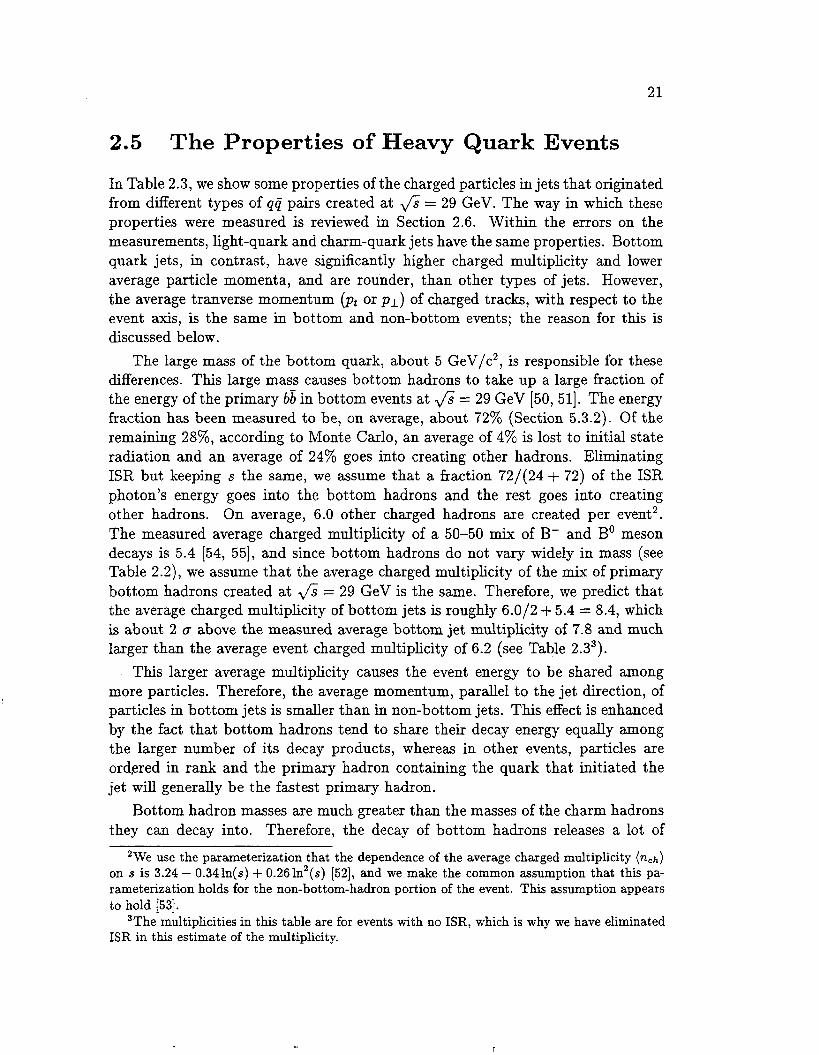
Electrons are ionized from gas molecules in two ways, depending on the amount of energy transferred to the gas molecule. For small energy transfers, the ionization cross-section is peaked at the electron binding energy, and since small energy transfers are most probable, this is the most important mechanism for energy transfer. For large energy transfers, the gas electrons are basically free and the process is described by Rutherford scattering. Rutherford scattering is relatively rare, but contributes a lot of ionization energy through these rare scatters (the so-called Landau tail in Figure 4.1), so the total ionization has large statistical fluctuations. To reduce these statistical fluctuations, the average of the smallest 65% of the individual wire dE/dz measurements is used as the measure of dE/dz. This is called the truncated mean, or the “dE/dz” of a track.

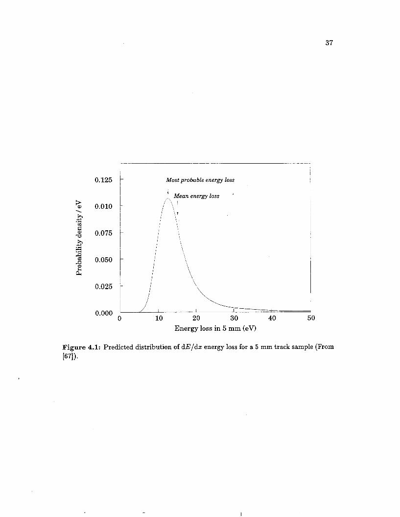
The dependence of dE/dz on Py is shown in Figure 4.2 [83]. For slow-moving particles, dE/dz c( l/p2, and dE/dz drops sharply with increasing p. This behavior is due to the fact that when the particle moves slowly, it spends more time near gas atoms and is more likely to ionize them, and this effect diminishes in strength as ,O increases. dE/dz reaches a minimum at around ,Or = 3, which is called the minimum ionizing region. ,L3r between 3 and about l o3 is called the relativistic rise region, where relativity enhances the particle’s transverse electric field and its ability to ionize the medium, causing dE/dz to rise slowly with ,By. In the Fermi plateau region, above @-y M lo3, the curve flattens out as the medium polarizes in response to the transverse field, cutting off any further increase in ionizing power [84, 851.

,&y is not directly measured, however, momentum is. p = P-ym implies lo&) = log(py) + log(rn), so when dE/dz is plotted as a function of log@) for different particle species, the curves for different species are simple translations, with respect to log(p), of the same curve that traces how dE/da: depends upon log(P7). The theoretical dependence of dE/dz upon ,By in the TPC has been calculated elsewhere, and fitted to data [25] . The fit is excellent.

The measured mean dE/da: also varies with time, dip angle, and TPC sector. These variations are corrected for by calculating how the average dE/da: for minimum ionizing pions depends on these quantities [25 , 861.

37

0.125

% 0.010 \

h L3 . i a 0.075

0.025

0.000 0

Most probable energy loss

I

\ \

I I I

10 20 30 40 50 Energy loss in 5 mm (eV)

Figure 4.1: Predicted distribution of dE/ds energy loss for a 5 mm track sample (From ~371).

38

I ~ \

Fermi Plateau I 20 r

Minimum-ionization region

I I

I I I I ! / l I I I l l l l l l i 1 I I I I I I 1 I l \ l l K i I I l l ] ! ! I 1 I I I I l I I

0 ' 1 10 10 10 10 10

?I =Pr Figure 4.2: Dependence of (dE/dz) on 17 = Py (From [67]).

39

4.3 dE/dx Resolution Parameterization

Each track has only a finite number of dE/da: samples, therefore experimentally measured values of dE/da: have a fmite resolution and form bands about the theoretical curves. Figure 4.3 shows that these bands sometimes are not well separated, particularly at high momentum and near the points where the theoretical curves cross. In these regions, tracks can not be unambiguously associated with only one dE/da: curve and can not be assigned a unique particle identification. We can still statistically determine the number of tracks with each particle identification, because we know the behavior of the dE/da: resolution, which we now describe.

The resolution has a Gaussian distribution out to at least 3 standard deviations [25]. For a sample of minimum ionizing pions from the High-Field data set with at least 120 wire hits, the resolution is 3.4%' [25]. The resolution varies with time, the number of wires with dE/da: samples ( N ) , and I sin XI.

We now describe the method used previously to find the parameterization for how dE/da: depends on N and I sin XI [25]. To take into account time variation in the resolution, the time in which the TPC collected the High-Field data set was divided into 10 intervals2 in such a way that the samples of minimum ionizing pions within these intervals are approximately the same size. Each sample was analyzed separately. For each sample, the standard deviation g of the quantity

measured Trmean(p,,,) expected Trmean (ptpc)

R = (4.4)

was computed and histogrammed as a function of N (ptpc is the momentum in the TPC). It was found that the parameterization Jm, with A and B free parameters, fits this plot pretty well. On average, A is 0.105 and B is 3.6 x 4- is the dependence of ~7 on the number of measurements, while the B term could be an intrinsic resolution added in quadrature to d%. What was then

done was to compute and histogram the standard deviation of ( R - 1)/4- as a function of 1 sin XI, in several histograms each with a different range of N . It was found that each histogram was well fit by a line, but the y-intercept of the fitted line varied with N . The end result was the parameterization

a ( ~ , A > = J A / N + B (C + DN + E ! sin XI) . (4-5)

C was found to be 1.17, D was found to be -7.2 x and E was found to be -0.28.

'For the Vertex Chamber data set, which is not used in this analysis, the corresponding sample of pions has a dEldx resolution of 3.1% [25, 861, the improvement due to better monitoring of the TPC.

2The Vertex Chamber data set was divided into 5 intervals.

f

40

1

60

55

50

45

n

I I I I I I

X

Pl rd 30 F

I I I I I I I I I I I I l l l l

25

20

15

10

10 -l 1 10

p (GeV/c)

Figure 4.3: Distribution of a sample of tracks in dE/dx as a function of lo&), with the predicted curves for e, p , 7r, K, and p (F'rom [67]).

41

This previously used method of parameterization contains a subtle but important oversight. The scatterplot of the High-Field data set pion tracks in the N-I sin A / plane at large I sin XI (Figure 4.4) has a diagonal concentration of tracks3, therefore the distribution of tracks in N is not independent of the distribution of tracks in I sin XI. As a result, the standard deviation as a function of N only, with the dependence on I sin XI projected out, does not find how the resolution depends on N as desired. Instead, the standard deviation with its dependence on I sin XI projected out is influenced by the variation of the resolution along the concentration of tracks at large I sin XI. The end result is that the best fit of a Gaussian to the distribution of ( R - l)/a(N, A) for all pions with 40 or more wire hits has a width of 1.1053 k 0.0038, which is more than 27 standard deviations larger than the expected value of 1, so the particle ID x2 values are 10% too big, on average.

160

140

120

100

80

60

40

20

I I I I I I I I I

0.0 0.1 0.2 0.3 0.4 0.5 0.6 0.7 0.8 0.9 1.0

I s inh j

Figure 4.4: Scatter plot of N , the number of wire hits, as a function of [ sinXI for minimum ionizing pions.

To fix this problem, the old parameterization of Equation 4.5 is fit in N and

3This concentration is produced by the fact that for 1x1 greater than 4 2 O , tracks coming from the Interaction Point can not leave ionization electrons on all of the 183 sense wires, since the ionization of that portion of a track with /zI > 0.9 m is absorbed by the gating grid. As a result, these large-dip tracks can not deposit charge on all of the 183 wires, only a subset, but most tracks will deposit charge on most of the wires accessible to the ionization electrons.

42

I sin AI simultaneously. In this fit, N is restricted to be greater than or equal to 40, since the resolution of the data for N less than 40 is systematically lower than the fit. The N-I sinA( plane was divided into rectangular bins, and a(R) in each bin was obtained with a maximum likelihood fit of a Gaussian to the distribution of R in that bin. Then a ( N , A) was calculated at the “center of gravity” of the data in each bin and fit to the a(R)’s, using a x2 fit. The standard deviation of the o(R) in each bin is a(a(R)) = a(R)/&, where n is the number of tracks in the bin. This expression for a(a(R)) is biased, however, since a small value of a(R) makes the standard deviation of a(a(R)) small also. Instead, we use a(a(R)) = a(N , A)/&.

When the fit of a(N,X) is done in this manner, B and D in Equation 4.5 are zero, within statistics, for both the High-Field data set and the unused Vertex Chamber data set. The fit is good. B and D were set to zero, and the fit redone with the resolution parameterized by

C + El sin A ( f i ’

a(N,X) =

which is much simpler than the original form. On average, C was found to be 0.474 and E was found to be -0.146 for the High-Field data set4.

The new parameterization we use does not suffer from the problems of the old parameterization: when ( R - l ) / a ( N , A) is plotted for all pions with 40 or more wire hits, the best fit Gaussian has a width of 0.9989 i 0.0034 (Figure 4.5), which is statistically compatible with the expected value of 1.

4For the Vertex Chamber data, on average, C was found to be 0.440 and E was found to be -0.100.

43

10

-3 E

+ 2 u+ 10 0 w aJ P E

10

1

Figure 4.5: Number of minimum ionizing pions (with N 3 40) as a function of (R - l)/a(N, A) (points with statistical error bars), with a Gaussian fit (solid).

T

44

Chapter 5

Event Reconstruction, Selection, and Simulation

In this chapter, we describe the more basic tools we use to do this analysis on the collected data. First, we outline the processing of raw data into reconstructed events. Then, we describe the selection criteria for removing backgrounds to the signal process e+e- --$ qQ -+ hadrons. Finally, we describe the Monte Carlo package used to simulate the experimental data and the tuning of this package so that it properly simulates experimental data.

5.1 Event Reconstruction

The TPC electronics, described in Chapter 3, produce a large amount of raw data that must be reconstructed into the events that produced the raw data. The reconstruction of events is done by a set of programs 1871 that processes ADC counts into space points, associates space points and wire hits with charged particle tracks, calculates the dE/dz of tracks from wire hits, makes particle identification assignments, fits tracks to a common event vertex, and removes cosmic ray tracks from the data. The end product of the event reconstruction are Data Summary Tapes (DSTs) that list the fitted tracks and their characteristics. Raw data is excluded from the DSTs.

5.2 Event Selection

When electrons and positrons collide in the PEP ring, they interact in a variety of ways, including annihilation into p+p-, T+-T-, or qij pairs, Bhabha scattering (e+e- -+ e'e-), and 2-photon processes (e+e- -+ e+e-yy and yy -+ X, where X

45

= anything). This analysis is only concerned with the process ese- --+ qq, so we need to filter out, as much as is practical, events due to the other processes.

The standard Good Hadronic Event Selection used in all TPC analyses of the process efe- --f qq is done by a program called LabelHadron-v2, which uses as its input the DSTs produced at the end of the data reconstruction. The selection criteria take advantage of the typical characteristics of hadronic events: large multiplicities, large energies, and low boost of the final state’s center of mass. Only charged tracks are used in this selection, and they must have these characteristics:

1. The dip angle 1x1 of the track must satisfy the constraint 1x1 < 60°, to ensure that the track enters the TPC fiducial volume.

2. Either dC < 0.30 GeV-l or dC/C < 0.30, where C is the track’s measured curvature, and dC is the error on the measured curvature. This ensures that the track is well measured.

3. The track momentum in the TPC volume must be > 100 MeV/c, and the track momentum extrapolated to the interaction point must be > 120 MeV/c. This ensures that the track has enough energy to have come from the event vertex.

4. The track must come from within 6 cm of the nominal vertex in the x-y plane and from within 10 cm in z , where the nominal vertex is the average vertex position for a period of roughly a few hours. This rejects tracks coming from cosmic rays or from interactions of particles with atomic nuclei in the beampipe.

Tracks that satisfy these criteria are called good tracks. To pass the Good Hadronic Event Selection, an event must satisfy these criteria:

1. There must be five or more good tracks that are not electrons. The electron identification is done either by dE/da: or by an algorithm that identifies pairs of tracks as coming from photon conversions. This rejects showering Bhabha events and low multiplicity event?, including ~ 1 + 3 events’.

2. The total energy of the good tracks, Echarged, must be > 7.25 GeV. This rejects 2-photon and beam-gas events.

3. The reconstructed event vertex must be within 2 cm in the z-y plane and within 3.5 cm in z of the nominal vertex. This rejects beam-gas events.

~

1“1+3” signifies that one r lepton decays into a final state with 1 charged particle and the other decays into a final state with 3 charged particles. 97.8% of i- events have 4 or fewer charged particles in the final state [SS].

46

4. At least one hemisphere of the event, as defined by the plane perpendicular to the sphericity axis, must contain either

(a) four or more good non-electron tracks or

(b) good tracks with an invariant mass greater than 2 GeV/c2.

This criterion rejects 714-3 events.

5. To reject 2-photon, beam-gas, and energetic ISR events, all of which usually have a large momentum imbalance in the z direction, the sum of the z-component of the momentum for all tracks, Cpz , must satisfy I C pz I < 0 . 4 E c f i a r g e d -

6. At least half of the tracks must be good tracks, to eliminate problematic events.

Monte Carlo simulation of the process e4e- ---f qij (discussed in the next section) shows that this set of selection criteria rejects approximately 32% of the ese- +

qij events. For the High-Field data set, 25189 events satisfy these selection criteria.

In this analysis, we use two additional selection criteria to ensure that the bulk of each event enters the fiducial volume of the TPC:

1. The sphericity axis of the event must be more than 45” from the beam direction.

2. The sphericity of the event must be less than 0.5, to ensure that the direction of the event axis is meaningful.

19529 events satisfy these additional selection criteria, as well as the Good Hadronic Event Selection.

Previous Monte Carlo studies have estimated that, of the events that pass the Good Hadronic Event Selection, (0.4&0.1)% are T events and (0.5fO.1)% are two- photon events [81]’. To remove these 7 and 2-photon events, we use the additional ‘7-27’ selection on events containing fewer than 9 good hadrons:

1. To remove r events, we discard events with an event thrust greater than 0.97.

2. To remove 2-photon events, we discard events with Echarged less than 9.5 GeV. A study [89] shows that essentially all 27 events have charged energy less than 9.5 GeV.

47

The motivation for using these two additional selection criteria is discussed in Section 5.3.3.4. We estimate that these two criteria remove 94% of all T events and 11% of the hadronic events that pass the Good Hadronic Event Selection. We have no estimate of the fraction of the 2-photon events that pass the good hadronic selection and are cut by these two selection criteria. 17943 events pass all of the selection criteria discussed in this section. The effect of all of the selection criteria upon the measured bottom event fraction is discussed in Section 7.4.3.

5.3 Event Simulation

5.3.1 The Event Simulation Software Package

In doing any analysis, it is important to simulate the physics processes that produce the observed events and the effects of the detector on the events collected. We use three programs for this simulation. Jetset 7.2 is used to generate simulated e'e- + hadrons events, except that we use the spring 1992 version of the CLEO Monte Carlo (described below) to simulate the weak decays of charm hadrons and bottom mesons.

Jetset 7.2 implements the Lund string fragmentation model, as described in Section 2.4.2, with parton showers. The Lund Symmetric Fragmentation Function (LSFF) does a fine job of reproducing the distributions of simple variables (such as sphericity, thrust major, charged multiplicity, and track momentum) for all hadronic events. However, the LSFF is unable to reproduce simultaneously the distributions of these variables, the average momentum of charm hadrons, and the average momentum of bottom hadrons [46]. This is unacceptable, since our analysis requires an accurate simulation of bottom, charm, and light quark events. Our solution is to use the LSFF only for light quark events, and to use the Peterson function, described in Section 2.4.4, for charm and bottom events. The Lund Monte Carlo uses a number of free parameters to determine how it hadronizes events, so these parameters must be tuned before Jetset is able to reproduce important characteristics of experimental data. The parameters that govern hadron flavor production, including production of bottom and charm hadrons, have already been tuned to data. Table 5.1 lists the valoes of those flavor parameters that are different from the default values [go]. The tuning of the parameters that govern event shape is discussed in Section 5.3.3.

The portion of the CLEO Monte Carlo used to simulate the decays of charm and bottom hadrons is an up-to-date decay table, which is a list of exclusive and inclusive decay modes, along with their branching ratios and decay matrix elements. This list instructs the CLEO Monte Carlo how to simulate charm and bottom hadron decays. The list contains all of the known exclusive decays, along with inclusive decay modes (e.g. b 4 cGd) that have been tuned so that the Monte

48

Tuned value 0.089 0.282 0.74 0.03 0.9

0.46 0.46 0.59

Default value 0.10 0.30 0.4

0.05 0.5 0.5 0.6 0.75

Table 5.1: Tuned values of the Lund flavor parameters in Jetset 7.2.

Carlo reproduces experimentally measured properties of charm and bottom decays. The CLEO Monte Carlo has been used for a long time and is known to reproduce the properties of bottom meson decays. We have verified that the CLEO Monte Carlo reproduces experimentally measured multiplicities and momentum spectra for charged pions, kaons, and protons from bottom meson decays, while Jetset does not.

TPCLUNDG, the standard fast TPC Monte Carlo, is used to simulate the TPC detector’s response to the events generated by Jetset 7.2 and the CLEO Monte Carlo. The output of these three programs are DSTs with the same format as experimental data. These output DSTs are subjected to the same hadronic event selection as experimental data. TPCLUND has been used for many years and is known t o accurately simulate TPC track measurements and the acceptance of the TPC’.

5.3.2 Tuning the Peterson Parameterization

As mentioned in Section 2.4.4, the Peterson function has one free parameter, E . Let TE = E/Ebeam, where E is the energy of the charm or bottom hadron in question, and let ( z E ) ~ and ( z E ) ~ be the average ICE for primary bottom and primary charm hadrons, respectively. E for charm events, E , , must be adjusted so that the Monte Carlo generated ( x z . ~ ) ~ matches the experimentally observed ( S E ) ~ . Likewise, E

’The previous version of TPCLUND, version 5 , was mated to Jetset 5.3 and 6.3. The structure of the programming of Jetset, especially the common blocks, is substantially different from that of Jetset 7.2. Rather than restructure TPCLUND to follow this change, the mating of TPCLUND to Jetset 6.3 was retained and the features of Jetset 7.2 that differ from Jetset 6.3 were copied into our now custom version of Jetset 6.3. As a result, when we refer to specific locations in the Jetset common blocks, we use the Jetset 6.3 locations.

.. .

49

Quantity (ZE) + 2 c ~ error (XE) central value

for bottom events, Eb, must be adjusted so that the Monte Carlo generated ( Z E ) b

matches the experimentally observed ( 2 E ) b .

Numerical values of ( z E ) ~ and ( z E ) , have been obtained from the plots in Reference [49] and are listed in Table 5.2. A 1-0 error of f0 .002 is assigned to these numbers from the uncertainty in the method used to read these values from the plots. We also assign an error of f0.03 [92] to these numbers to reflect the statistical and systematic uncertainties on ( Z E ) b and ( z E ) ~ in Reference [49].

Charm Bottom 0.586 0.775 0.526 0.715

1 ( X E ) - 20 error 1 0.466 I 0.655 I Table 5.2: ( Z E ) b and (zE), from Reference [49].

Table 5.3: Eb and E, for Jetset 7.2.

In Table 5.3 are listed the values of Eb and E, in Jetset 7.2 that reproduce these VdUeS Of ( Z E ) b and ( I C E ) , .

5.3.3 Tuning the Jetset Event Shape Parameters

The Lund parameters to be tuned govern the shape and momentum structure of Monte Carlo-generated events. They are:

3P(qq)/P(q) is the diquark to quark probability ratio in breaking the string. P(s) /P(u) is the ratio of strange quark to up (or down) quark production. [P(su)/P(du)]/[P(s)/P(u)] is the probability of creating an su-diquark versus a du-diquark, relative to the ratio P(s) /P(u) . P(ud1) and P(ud0) are the probabilities for the creation of a spin-1 and a spin-0 diquark, respectively. P ( B M B ) / P ( B M B + BB) is the 'popcorn' baryon production [91] probability, where the meson M is created between two baryons B in string fragmentation. P(vector)/P(aZE) is the fraction of mesons produced that are vector.

50

1. the a and b parameters in the Lund Symmetric Fragmentation Function (Section 2.4.2),

2. AQcD, the QCD scale parameter described in Section 2.3,

3. gg, the width of the Gaussian p , distribution (Section 2.4.2), and

4. the parton shower virtuality cut-off QO described in Section 2.3.2.

The vector to pseudoscalar ratio T also affects event shape, but it is fixed at the value determined by vector meson production measurements.

The Peterson parameters tuned in the last section are weakly correlated with AQCD and Qo. This implies that the optimization of the 5 Eund parameters listed above throws off the optimization of the Peterson epsilons. In principle, therefore, it is necessary to tune the Lund parameters and the Peterson epsilons alternately until they all converge. It turns out that the tuning in this section changes ( z E ) ~ and ( Z E ) ~ by much less than their errors, so the Peterson epsilons need not be retuned.

The procedure used here for tuning the Lund model parameters in Jetset 7.2 largely follows the procedure used to tune Jetset 5.2 [78], which produces distributions of a set of variables in data aild in Monte Carlo and minimizes the differences between the two sets of distributions. We now describe the procedure used to tune Jetset 5.2. After that, we describe the procedure we used to tune Jetset 7.2.

5.3.3.1 The Kinematic Variables Used for Tuning.

We first describe the variables used to tune Jetset 5.2. These variables are listed in Table 5.4. Q1 and QZ are the smallest and next smallest eigenvalues of the sphericity tensor3. L1 and L2 are the thrust minor and thrust major, respectively4. ( p l i , ) and pi)^,, are the average momentum per event and the momentum per

3The sphericity tensor is given by

where pg is the a-component of the momentum for track i. 'The thrust major and thrust minor are defined as follows. First, define

where n' is a unit vector. The thrust L3 is the maximum of T , and the thrust axis is the vector n' = n'l that maximizes T. The thrust major axis n' = Z2 is the vector perpendicular to iil that maximizes T, and this maximum of T is the thrust major La. Finally, the thrust minor axis 8 3

is perpendicular to 81 and 5 2 , and the corresponding value of T , L1, is the thrust minor.

51

XP Charged Multiplicity

track in the event plane (as defined by the sphericity tensor) and perpendicular to the sphericity axis. (pout) and (pi)out are the average momentum per event and the momentum per track out of the event plane (as defined by the sphericity tensor). xp = p/pbeam, where p is the momentum of a track. is the difference between the squared masses of the the two jets in the event, as defined by the plane perpendicular to the sphericity axis. &is is the visible charged energy of the event.

Q i

L1 ( P l O U t )

(pi)lout

Set 1 Set 2 I Set 3

Table 5.4: Variables used for tuning.

The quantities in Set 1 are most sensitive to hard gluon radiation, so they are sensitive to A Q ~ D , which controls the rate of hard gluon radiation. The quantities in Set 2 reflect the hardness of the fragmentation, and thus are sensitive to the Lund a and b parameters. The tuned values of a and b are highly correlated, so b was fixed and a was tuned. The quantities in Set 3 measure the thickness of the event out of the event plane, and thus reflects oq. We use the same variables to tune Jetset 7.2.

5.3.3.2 The Old Tuning Methods.

The method for tuning Jetset 5.2 used two sets of histograms: one set was the distribution of the number of events or tracks as a function of these tuning variables for experimental data, and the other set the corresponding distributions for Monte Carlo. These two sets were compared to each other using two different methods.

In the first method, for coarse tuning, we calculate a x2 to compare the experimental and Jetset/TPCLUND distributions. Let Dij be the number of experimental data entries in bin i of distribution j, and let Mij(p3 be the number of entries in bin i of distribution j from our Monte Carlo with parameter set 5. After normalizing the data and Monte Carlo histograms to the same number of entries,

a(sys) is an estimated systematic error, set equal to a constant fraction, Fsys, of Mij. This fraction, which is 5% in the tuning of Jetset 5.2 and 2% in the tuning

52

of Jetset 7.2, is set so that the best tune’s X2/bin is approximately 1.0. Fsys is smaller for Jetset 7.2 because parton shower Monte Carlos such as Jetset 7.2 are better at reproducing experimental data than fixed order QCD Monte Carlos such as Jetset 5.2.

We can calculate this x2 for a variety of Monte Carlo parameter settings. For instance, we can choose to vary only one parameter at a time in order to obtain a crude optimization of the Lund model parameter set.

In this measurement, we tune in 5 parameters, and using this method to search for the minimum of x2 in this 5-dimensional parameter space, to several significant figures, would be time-consuming. Therefore, in order to obtain a fine tuning of the Lund model parameter set, along with an estimate of the associated systematic errors, a second method was used for comparing experiment to Monte Carlo. Instead of comparing experimental distributions to Jetset/TPCLUND distributions, this method unfolds the effect of detector acceptance on the experimental distributions and “fits” Jetset distributions (no TPCLUND) to these unfolded distributions, with bin entries Dij.

The unfolding is accomplished by using a preliminary Lund parameter set, which we label $0, to generate a set of Jetset/TPCLUND distributions and a set of Jetset-only distributions. The ratio of the two distributions is used to unfold the experimental distributions.

The “fitting” is done as follows. A second set of Jetset distributions is generated using the preliminary parameter set 9 0 (the so-called expansion point). In addition, one parameter at a time is varied to each side of that parameter’s preliminary value, and a set of distributions is generated at each of these points. Using these distributions, we can approximate the number of entries Mij in each bin in each distribution as a first order Taylor expansion in the parameter space p’:

The spacing of the parameter sets around the expansion point must be fixed at values that are not too small. Otherwise, the difference in the contents of some bins becomes smaller than the error in this difference, creating large random variations in the coefficient of 9- $0 in the second term of Equation 5.4 that tend to exaggerate greatly the growth of Mij(p3 as 16- $01 increases. If this happens in many bins, then the minimum of x2 is forced to be artificially close to p’o, with unreasonably small errors on this minimum.

We substitute Equation 5.4 into Equation 5.3 and solve for the parameter set that optimizes x2. Instead of summing over all 11 distributions, the old method summed over three distributions, one distribution chosen from each of the three sets of distributions in Table 5.4. Then x2 was computed 40 times, for the 40 = 5 x 2 x 4

.. .

53

possible combinations of three distributions. The total x 2 per bin is a measure of the goodness of the fit, the average of the 40 parameter sets is the new parameter set selected by the fit, and the r~ of the 40 parameter sets is the systematic error of the parameter set.

In general, this new parameter set is not equal to the expansion point’s parameter set, so this fitting process must be iterated, substituting this new parameter set for the old parameter set. This process is repeated until the change in the parameter set from one iteration to the next is less than the systematic error on the parameter sets.

5.3.3.3 Modifications to the Old Method.

A difficulty with the old fine tuning method is that convergence in the average of 40 parameter sets does not imply convergence in the individual parameter sets. The method used here combines all of the histograms in one of the 3 sets of histograms into a superhistogrum, for all 3 sets, and the sum in Equation 5.3 is done over the 3 superhistograms. The tuning is then iterated until it is clear that the parameters are fixed, apart from statistical fluctuations whose size is estimated in the tuning. We consider the spread in the 40 parameter sets, as evaluated in the old method, a good estimate of the systematic error.

The old method ignored g2(M;j) in Equation 5.3, thus making it possible to solve for the minimum in x 2 using a system of linear equations. The method used here does not ignore this contribution to the error. Taking this contribution into account sometimes causes the minimum of x2 to correspond to physically absurd parameter sets, due to statistical errors in Equation 5.4. This pathological behavior is cured by using the common trick of finding the minimum of x2 in a stepwise manner. In each step, x2 is minimized with a2(Mij) fixed at the value calculated using the $determined in the previous step. For the first step, the expansion point $0 is used to calculate g 2 ( M ; j ) . This process is repeated until @converges, typically after 4-6 steps.

This method should give the same value of $ as the coarse tuning method discussed above if enough time were spent on the latter method. We do not attempt to do a fine tune using the coarse tuning method.

5.3.3.4 Backgrounds.

There is an additional pitfall in the tuning: backgrounds. The r and 27 backgrounds are estimated to be approximately 1% of the good hadronic event sample, so one might naively think that backgrounds can be ignored. They can not be ignored because they are concentrated in small regions of some of the tuning distributions where there are not many hadronic events. r and 27 events have low

54

multiplicities, so those 7 and 2y events that pass the hadronic event selection cluster in the lowest bins in multiplicity. 7 events, because of the low 7 mass, are highly collimated and back-to-back, so they also cluster at large thrust, low thrust major, and low thrust minor. During the tuning procedure, before the 7-27 selection was implemented to eliminate these backgrounds (described in Section 5.2), data clearly showed a statistically significant excess over Monte Carlo for multiplicities of 5 and 6, and especially for the lowest bins in thrust minor where there are essentially no hadronic events. A less significant excess was seen at low thrust major.

We did not try to simulate these backgrounds for two reasons. First, the simulation of 27 events is difficult. Second, according to TPCLUND6, approximately half of the r events that passed the Good Hadronic Event Selection have nuclear interactions, and the TPCLUND nuclear interaction simulation is not considered very reliable.

The alternative to simulating these backgrounds is to cut them. To avoid losing information for the fitting, we did not remove from the fit those bins where the backgrounds are important. Instead, we decided to eliminate the backgrounds by designing selection criteria in variables designed especially to remove these backgrounds. The resdt is the 7-27 selection of Section 5.2.

TPCLUNDG estimates that the 7-27 selection removes 94% of all r events that pass the good hadronic selection, 37% of the passing hadronic events with 8 or less good hadrons, and 11% of all the passing hadronic events.

The 7-27 selection removes or makes statistically insignificant the previously mentioned differences. Figure 5.1 shows the differences, in standard deviations, between tuned Monte Carlo and Experiment 14-18 data before and after the 7-27 selection was implemented. The tuned parameters did not change a large amount after the 7-27 selection was implemented, which is not surprising, since few bins were affected. However, the X2/bin, with the systematic error floor Fsys = 2%, dropped from about 1.2 to about 11.0.

5.3.3.5 Results of the Tuning.

For the tuning of Jetset 7.2, b was fixed by tuning it so that Jetset reproduced the TPC D* momentum spectrum. The D* spectrum is now controlled by E , , so we can and do tune both a and b. In fact, we have simultaneously tuned AQCD, Qa, a, b, and cq with two different values of the systematic error floor Fsys: 2% and 0%. The results are in Table 5.5, and histograms of the number of events or tracks as a function of the the tuning variables for experimental data and for Monte Carlo with Fsys = 2% are in Figures 5.2 through 5.4. The tune with Fsys = 2% is our best tune of the Monte Carlo. We use the tune with Fsys = 0% for estimating systematic errors.

The optimizations were well-behaved.

1

55

25

20

15

10

5

0 10 20 30 40

Multiplicity

2 fi 5 n 2 5 Gi

.O 12.5

.*

P 10.0

-0

7.5 1 5.0

2.5

0.0 0.0 0.2 0.4 0.6

Thrust Major

Thrust Minor

Figure 5.1: Absolute value of the discrepancy, in standard deviations, between Monte Carlo and Experiment 14-18 data without (solid) and with (crosses) the 7-27 selection for multiplicity N (a), thrust minor L1 (b), and thrust major Lz (c).

56

Fsys Parameter

2% .364 f .022 1.360 z t .129 .053 f .051 .497 f .071 .320 f .006 0% .317 f .016 1.870 f -346 -385 f .049 -632 f -055 .336 f .005

AQCD Qo a b flq

x2 / bin

0.94 1.33

0.00 0.04 0.08 0.12 0.16 0.20 0.24 0.28

1.5 Q1

lo3 5 > U “0 l o 2 L1 0, P g 10 z

1

0.0 0.1 0.2 0.3 0.4 0.5

Thrust Minor

m Y

i! U

0

P

YI

8 E 5

m + 5 >

W

0

P

YI

8 E z

lo3

lo2

10

0.0 0.1 0.2 0.3 0.4 0.5 0.6 0.7

lo3

lo2

10

1

0.0 0.1 0.2 0.3 0.4 0.5 0.6 0.7

Thrust Major

Figure 5.2: Experimental data (points) and tuned Monte Carlo (solid) histograms of the number of events as a function of the aplanarity 1.5Q1 (a), 1.5Q2 (b), the thrust minor L1 (c), and the thrust major L2 (d).

57

(I) lo3

* IO2

M n E 10

Y

2 w 0

5 1

0.0 0.1 0.2 0.3 0.4 0.5 0 4 8 12 16 20 24 28 32

m2jet / E’, Charged Multiplicity

0.0 0.2 0.4 0.6 0.8 1.0 0.0 0.1 0.2 0.3 0.4 0.5

( pLin>. GeV/c ( PI out >I GeV/c

Figure 5.3: Experimental data (points) and tuned Monte Carlo (solid) histograms of the number of events as a function of AM$t/I?:i, (a), Charged Multiplicity (b), ( p l i n ) (4, and h m t > (4-

.. .

58

10 ‘ 0.0 0.4 0.8 1.2 1.6 2.0 2.4

10 0.0 0.2 0.4 0.6 0.8 1.0

0.0 0.2 0.4 0.6 0.8 1.0

P / Pbearn

Figure 5.4: Experimental data (points) and tuned Monte Carlo (solid) histograms of the number of tracks as a function of (pi)i in (a), ( p i ) l m t (b), and xp (c).

59

The big difference between the 2 sets of parameters is that Lund a and b are higher for the tuning with the 0% systematic error floor than for the tuning with the 2% systematic error floor. The reason this happens is that the track momentum spectrum for xp > .14 is best fit by small values of a and b, while xp < .14 is best fit by larger values of a and b.

The momentum is binned in equal intervals in xp, thus most of the bins have xp > .14, but these bins contain only 19% of the tracks, as shown in Figure 5 .4~ . The higher statistics for bins with xp < .I4 favor these bins, while the greater number of bins for xp > .14 favors these bins. Tuning with a 2% systematic error floor dilutes the weighting of the high statistics for xp < .14, so the 2% tune fits xp > .14 better than xp < .14, resulting in small a and b. Tuning with a 0% systematic error floor does not dilute xp < .14, resulting in larger a and b.

60

Chapter 6

Feed-Forward Neural Networks

In this chapter, we describe the design, training, and use of feed-forward neural networks'. We also describe some relevant prior applications of feed-forward neural networks to high energy physics. In Chapter 7, we describe our use of a neural network to measure u(b6)/u(@), and in Chapter 8 we describe our use of a neural network in a study of bias in measurements of charged hadron production in bottom jets, where neural networks are used to tag the bottom-quark jets.

6.1 Neural Network Architecture

A feed-forward neural network is pictured as a layered array of nodes with a connection between each pair of nodes in adjacent layers, as shown in Figure 6.1. We shall use as a general example a network with three layers: an input layer (the bottom row of nodes in Figure 6.1), an output layer (the top row), and one hidden layer (the middle row). A network can have any number of hidden layers, including zero. It has been shown that there is nothing to be gained from having more than two hidden layers, and that one hidden layer is often sufficient [94, 951.

Each node represents a number: zk for node k in the input layer, hj for node j in the hidden layer, and y; for node i in the output layer. For a general, type of analysis, where one wishes to classify an N-dimensional vector as belonging to one of L classes based upon differences in how the classes are distributed in the N-dimensional space of all vectors, one has N nodes in the input layer, each node representing one of the components of the vector. Each input N-tuple is called a pattern.

'Reference [93] is a recent review of neural networks, accessible to readers without previous knowledge of neural networks, along with an extensive bibliography and a guide to the neural network literature.

61

W i j

h j

w j k

xk . . . . .

Figure 6.1: A one hidden layer feed-forward neural network architecture (nom [ S S ] ) .

The M output nodes are used to classify the input pattern. For a one output network, the value of the output is a simple yes (1) or no (0) if the classification of the input pattern is certain, and in between 0 and 1 if the classification is uncertain. For more than one output node, each output node's value can encode one bit of information in an M-bit binary word representing the network's classification of the input pattern, and the network can make 2M classifications. Alternatively, each node can represent one of M classifications: the output node representing the assigned classification is 1 and all of the other nodes are 0. In any case, each classification of the input pattern has a corresponding target output M-tuple

We now describe how the values of the numbers represented by each node are set. The values of the numbers in the input nodes are set equal to the values of the corresponding components of the pattern being presented to the network. In the other layers, the number in each node in a particular layer is a function of the numbers in all of the nodes in the previous layer. For the output layer, this function is

(Yl, " ' 7 YM) = (tl, " ' 7 t M ) .

r -

while for the hidden layer, the function is

where T is the network temperature (an inverse gain), w i j (wjk) is the weight (or strength) of the connection between nodes i (j) and j ( I C ) , Oi (ej) is the threshold for

.. .

62

node i ( j ) , and g(a) is a non-linear transfer function. Typically, transfer functions asymptotically approach a fixed value for argument a + 03 and another fixed value for a --+ - m, a common choice is g(a) = tanh(a). In this fashion, numbers are propagated forward through the network from the input layer to the output layer, hence the name of this type of network: feed-forward.

In Equations 6.1 and 6.2, the argument of g is a linear function of the values of the nodes in the previous layer. When this argument, Oj + Ckujkzk, is set equal to a constant, it defines a hyperplane in the space of vectors defined by Z = (zl, . . . , zk , . . .) . Therefore, a O-hidden-layer neural network maps regions of the input space bounded by hyperplanes to small regions of the space of outputs, and such networks are functionally identical to a linear discriminant. The non- linearity of g enables networks with at least one hidden layer to map regions of the input space with curved boundaries to small regions of the output space. Thus, neural networks are often more powerful than linear discriminants or other multi- dimensional classifiers [97].

6.2 The Training of a Neural Network

A neural network does not automatically classify the input patterns. The parameters (weights and thresholds) of the network must be set to values that enable the network to perform this task. The process in which these parameters are set is called training.

The most common method for training uses the back-propagation algorithm [98], which is used in this analysis. Training a network requires a training set of L equal-sized samples of patterns, one sample from each classification. Equal-sized samples are used so that the network does not favor one class over the others.

In the original off-line use of the back-propagation algorithm, the entire training set is presented to the an epoch. At the end to reduce the error

where &'I and -&) are P -

network repeatedly, each complete presentation being called of each epoch, the weights and thresholds are incremented

the calculated and target output values in node i for pattern

Suppose that there are n weights. The current value of these weights can be organized into an ordered n-tuple that is a point P in the real r-dimensional Euclidean space R" of all possible n-tuples. Then the rule for incrementing the weights is for the point P to move opposite the direction of the gradient of E in

1

63

the space of weights:

and

where 17 is the learning rate. The partial derivatives are easily calculated using the chain rule:

and

Similar formulae exist for the thresholds. The initial values of the weights and thresholds must be randomly chosen; otherwise, the training may have difficulty breaking the symmetry of the initialization (e.g. all parameters zero). Typically, these initial values are randomly generated uniformly in an interval [ - -wo, wo].

The weights and thresholds are repeatedly incremented in this way in a stepwise search for the minimum of E in the space of weights and thresholds, until E no longer decreases. There are ways of avoiding local minima [96]. In minimizing E , the actual network output M-tuple (91, ..., y ~ ) for each class of patterns is forced to be as close as possible to that class's target output M-tuple, and the different classes of patterns are separated from each other as much as possible. This is how the network gains its ability to distinguish the classes of inputs from each other.

In practice, on-Zine training is used. Instead of updating the weights and thresholds at the end of each epoch, small groups of patterns composed of equal-sized sets of randomly selected events from each class of patterns are presented to the network, and the network parameters updated after each group has been input. In addition, the updating formulae are changed to

and

to damp out oscillations. The new second term in these equations is a momentum term proportional to the increment of w in the previous update; t is the update number and CY should be between 0 and 1. On-line back-propagation better avoids local minima and is often faster than off-line back-propagation.

The decision about when to terminate training requires a test set, which is like the training set in that it also consists of L equal-sized samples of patterns, one

64

sample from each classification, but the patterns in the training and tests sets are different. What is important is not the network’s ability to classify the training set patterns, but rather the network’s ability to generalize what it learned from the training set to the task of classifying an independent test set’s patterns.

It often happens that the error E evaluated for a test set will decrease to a minimum and then actually starts to increase. This happens because, at first, the network is learning the general characteristics that distinguish the patterns in each classification from each other, but past a certain point the network learns the statistically random peculiarities that distinguish the training set’s classifications from each other. This is called overtraining. Overtraining is handled by increasing the size of the training set, thereby reducing statistical fluctuations and increasing the network’s performance on the test set. Increasing the size of the training set also decreases the performance on the training set towards the performance on the test set, since the network can not learn the training set’s peculiarities as readily. If the size of the training set becomes too small, then the network memorizes ‘individual patterns and the network’s ability to generalize plunges.

On the other hand, if the ratio of the number of training set patterns to the number of network parameters is too big, the probability of getting stuck in a local minimum during training increases. A good compromise between these competing demands is for this ratio to be on the order of 100 [99].

The issue of the choice of the number of nodes in each hidden layer can now be handled in several ways. There exist a variety of algorithms designed to be used to eliminate unnecessary nodes. A class of such algorithms are pruning algorithms, [96] which simultaneously train the network and set to zero the weights connected to unneeded nodes. Our experience shows that the number of nodes the algorithm decides to prune is not directly enough related to the pruned network’s performance. Instead, we take a direct approach: we see how the performance of the network varies as a function of the number of hidden nodes. Typically, the performance is seen to rise rapidly with increasing number of hidden nodes when this number is small (see Section 7.2). The performance then asymptotically approaches a limiting value as the number of nodes becomes larger. Measures of network performance besides E are discussed in the next section.

The traditional approach in High Energy Physics of doing analyses with a sequence of selections is equivalent to a structured decision tree, where decisions are made sequentially. In contrast, a neural network is a form of parallel computing. Each node in a network “votes” on the network’s decision. As a result, neural networks have two desirable properties that decision trees do not have 1991:

1. Robustness: a few bad inputs can be tolerated in decision-making.

2. Generalizability: networks respond to previously unseen patterns by gen- eralizing from what the network learned during the training process.

65

These properties, and the power and general applicability of neural networks, are the reason for the interest in neural networks in the field of High Energy Physics. On the other hand, the voting of the nodes means that individual nodes do not have specific functions. A network’s decision-making is spread among all of the nodes.

6.3 Measuring Network Performance

What we mean by a network’s performance is its ability to distinguish patterns from different classes. The usual measure of performance is the error E , but there exist other measures of performance. For example, with a one output network, it is common to calculate the efficiency and purity, as a function of a cut on the network output, for the signal patterns in the sample of patterns with outputs above the cut. We have chosen to use a compact measure of performance for a one output network that directly quantifies the statistical separation of the classes

This method, for the case of two classes ( L = 2 in the notation of Section 6.1), uses a set of signal patterns, a set of background patterns, and a data set composed of signal and background only. As an example, the signal is composed of bottom events, the background is composed of non-bottom events, and data is composed of a mixture of the two. We start out by producing neural network output distributions for these three sets of patterns. Then, a fit is done of a linear combination of the signal distribution and the background distribution to the data distribution, yielding the error on the fraction of the data that is fitted to be signal. Our measure of network performance is the dependence of this error on the overlap of the two distributions, with the dependence of the error on the finite size of the signal and background samples removed.

We work out what our measure of performance is mathematically. Binning the network output and labelling the bins i, let si, b;, and di be the fraction of the signal, background, and data (respectively) in bin i, let N be the number of data patterns, and let LY be the fraction of the data that is actually composed of signal. Then the x2 of the fit of a linear combination of signal and the background to the data is

[loo, 1011.

(as; + (1 - LY)bj - dJ2 x2 = N E i c2 (4)

(as2 + (1 - a)bz - di)2 = N E

a di (6.10)

66

The value of Q that minimizes x2 is

(6.11)

with

where we have defined

I

(si - bi)2 F = d ( l - & ) C rl

(6.12)

(6.13)

(6.14) i Ui

In Monte Carlo studies, we make the substitutions d = a and di = &si + (1 - d)bi. F is our measure of network performance. If we could achieve perfect separation

of signal and background (that is, each bin i has either si = 0 or bi = 0), then F = 1. If si = bi for all i, then F = 0. Otherwise, 0 < F < 1.

The generalization to more than two classes of patterns ( L > 2) is derived in Appendix B.

An example of an application of F is in Reference [loll , which compares the performance of networks with different types of inputs. One approach is to use, as inputs, ‘raw’ quantities such as particle 4-momenta, 3-momenta, or energy deposits in a calorimeter [99, 101, 102, 1031. The motivation for using ‘raw’ quantities is to provide the network with as much information as possible and to have the network extract the useful information.

Another approach is to use, as inputs, constructed shape variables that describe the event shape (e.g. thrust, sphericity, and thrust minor) that have different distributions for b and non-b events. The preprocessing of the information into these shape variables ought to make it easier for the network to extract the information useful for distinguishing b and non-b events. There are a large number of possible shape variables that can be used as inputs, so we can pick a small set of variables such that the network output distributions for b and non-b events are as well separated as possible [99, 101, 104, 105, 106, 1071.

The raw input approach keeps information that might otherwise be thrown away in the preprocessing approach. As a result, one might expect that networks with raw inputs perform better, but with the trade-off that raw input networks take much longer to train. For the examples studied in Reference [loll, these expectations are fulfilled. In this reference, the preprocessed 25-input network has F = 0.258 and the raw 23-input network has F = 0.312; both networks have one hidden layer containing 5 nodes.

67

6.4 Previous Uses of Neural Networks in High Energy Physics

Neural networks are increasingly being used in high energy physics [108, 109, 1101. Previous applications of back-propagation neural networks to high energy physics can be roughly divided into two groups: data compression for fitting in a network output, and classification.

6.4.1 Classification Using Neural Networks

In an example of this application, calorimeter information is used for inputs to a neural network, which attempts to determine what kind of particle generated the calorimeter information [lll, 112, 1131. There is one output for all of these networks. A cut is made on this output and all patterns that produce an output above this cut are classified as being produced by one kind of particle, while all other patterns are classified as being produced by another particle. Figure 6.2 shows the network output distributions for electrons and for hadrons for a network designed to distinguish these two classifications of particles [ 1111. These two distributions are well separated; for this sort of application the two output distributions must have little or no overlap.

6.4.2 Fitting in a Neural Network Output

Analyses in which the b6 width of the Zo is measured are the archetype of this approach. Here, a linear combination of the neural network output distributions for Monte Carlo b events and for Monte Carlo non-b events is fitted to the network output distribution for experimental data [114, 1151. Figure 6.3 shows the L3 Collaboration's fit and the distributions for b events and for non-b events. Both Monte Carlo distributions fill the entire range of network outputs, from 0 to 1, which is what happens when the network inputs do not carry enough information to distinguish unambiguously the two types of events. It may even happen that the output distributions do not cover the entire range from 0 to 1. This is the method used in this analysis to measure the fraction of hadronic events that are bottom events.

An inherent disadvantage of this type of analysis is the reliance upon Monte Carlo for training the networks. This reliance is necessary because there are no unbiased samples of b or non-b events available on which to train a network.

It is also possible to do this kind of analysis with three or more classes of patterns. The DELPHI Collaboration [116] has measured the bottom, charm, and light (up, down, and strange) quark widths of the 2' using a 3-output network.

68

80

60

40

20

0 0.0 0.2 0.4 0.6 0.8 1 .o

Network Output

125

100

75

50

25

0 0.0 0.2 0.4 0.6 0.8 1 .o

Network Output

Figure 6.2: Neural network output distributions for electrons (a) and for hadrons (b) for the DO neural network designed to distinguish the two (From [ill]).

.. .

69

5000 1

I.

0 3000 L

5 2000

1000

I l " " l " ' I " "

Data - Fitted MC total ___-. Fitted MC b

. . . . . . . .

0

Fitted MC non-b

-_ - - - - - _ _ ..--, , I I 1 , 1 1 1 ' , ~ ~ I .

0.2 0.4 0.6 0.8

Network Output

I ..'- 3+ . .. '....

I

Figure 6.3: L3 fit of a linear combination of the neural network output distributions for Monte Carlo b and Monte Carlo non-b events to the network output distribution for experimental data (From [115]).

70

Dalitz-type scatterplots of the output distributions are shown in Figure 6.4, with the sum of the three outputs normalized to 1. As discussed in Section 6.1, only two independent outputs are needed for this analysis. It is possible to use a 1-output network and fit a linear combination of three distributions, but it would not be possible to train the network to recognize the three classes of events. Instead the network would be trained on sets of b and non-b events and it would respond differently to charm and light quark events.

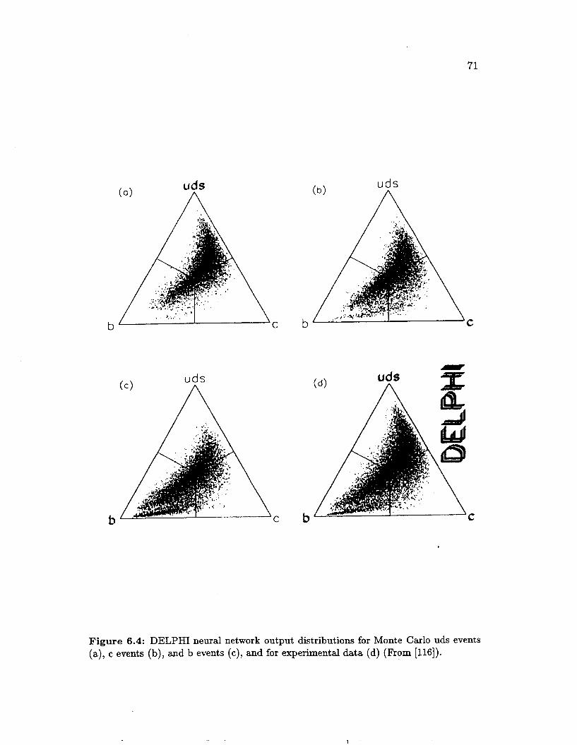
71

(0)

/ . \

uds A

b ’ I ‘ C b C

uds

b c b C

Figure 6.4: DELPHI neural network output distributions for Monte Carlo uds events (a), c events (b), and b events ( c ) , and for experimental data (d) (From [116]).

72

Chapter 7

A Measurement of the Bottom Event Production Fraction

The ratio a(b6)/a(q$ has never been measured in the continuum. Normally, the value of a(b$)/u(qq) is deduced from the discontinuity in R = u(qq)/a(p+p-) at the b6 threshold. In this chapter, we present a first measurement of the ratio a(bz)/a(qij) in the continuum. This measurement is based on 66 pb-' of TPC/2r data collected between 1984 and 1986, and it uses a neural network with inputs that are computed from charged hadron 3-momenta to distinguish b and non-b events.

In this chapter, we first describe the network's inputs and architecture, and how they were designed. Next, we show how the network was trained. We then describe and implement a method for fitting the bottom event fraction in the experimental data. We describe how the fitted bottom event fraction depends upon the Monte Carlo bottom event fraction, and we use a new method to extract a consistent bottom event fraction. Finally, we discuss our measurement of a(bE)/a(qij) and compare it to previous measurements of IT(Zo+ G).

7.1 The Choice of Neural Network Inputs and Architecture

For the event-tagging neural network we constructed to identify bottom events, we chose the preprocessed input approach discussed in Section 6.3, for the sake of simplicity. We compiled a list of candidate inputs and for each of them computed F (described in Section 6.3) , which quantifies how well the b and non-b distributions are separated. We selected 7 variables', uses a with relatively large values of F

IN = 7 in the notation of Section 6.1

73

that are fairly independent of each other. The selected variables, computed using the tracks and events that pass the selections described in Section 5.2, are:

I. N Ecm/Ewis, the scaled event charged multiplicity, where N is the number of charged tracks in the event and Euis is the event visible energy.

2. Cpf;"tEcm/Eu;s, the scaled sum, over all tracks, of the component of the track momenta perpendicular to the event plane, the plane defined by the thrust axis and the thrust major axis (these axes are defined in Sec- tion 5.3.3.1).

3. Cp;i" Ecm/E,,is, the scaled sum, over all tracks, of the component of the track momenta in the event plane and perpendicular to the event (thrust) axis.

4. Cpll Ecm/Ewjs, the scaled sum, over all tracks, of the component of the track momenta parallel to the event axis.

(1) (2) 5. M( l ) Ad2) E,2,/[4Ewis Ewis], the product of the scaled invariant masses of both hemispheres, where the hemispheres are divided by the plane perpendicular to thrust axis, M(;) is the invariant mass of hemisphere i, and E$? is the visible energy of hemisphere i.

6.

7. The boosted sphericity product S1 x S2, where Si is the sphericity of hemisphere i calculated in the frame of reference boosted by p = .47 along the event axis, in the direction of hemisphere i. p = .47 was chosen because it maximizes F for this variable.

x pil",', where p:;? is pll for the leading track in hemisphere i.

The distributions of these variables for b and non-b Monte Carlo events that pass the analysis selections are shown in Figures 7.1 and 7.2, and the values of F for the 7 inputs are listed in Table 7.1. Note that these variables take advantage of the differences between bottom and non-bottom events discussed in Section 2.5.

To help distinguish bottom events from 3-jet non-bottom events, we use as inputs p;i" Ecm/Ew;s and CpY' Ecm/Ev;s, since the latter is considerably smaller than the former for 3-jet events, which have a distinctly flat shape, whereas bottom events are more isotropic in the plane perpendicular to the event axis.

The boosted sphericity product, SI x Sz, also distinguishs bottom events from 3-jet non-bottom events. Bottom events have large SI x S,, since the tracks in each of the two hemispheres are largely produced by the roughly isotropic decay of a bottom hadron with a boost in the neighborhood of p = .47, giving S1 and S2 large values. In contrast, 3-jet non-bottom events often have one hemisphere

74

Input: 1 F : 0.080

2 3 4 5 6 7 0.100 0.155 0.120 0.130 0.058 0.129

with large S, since that hemisphere contains 2 jets, while the other hemisphere has small S, since it contains one non-bottom jet.

The inputs we use are these 7 variables after they have been linearly scaled so that the range of values for each input is 0 to I. If we do not scale the inputs, the neural network inputs can have significantly different ranges of values, and this can reduce the network’s performance. This reduction happens because the network parameters are normally initialized, before training has started, so that they are randomly distributed in a fixed interval, and if the ranges of the inputs are very different, training will favor some of the inputs [103].

To distinguish two classes of events from each other, the event-tagging network has one output. The target output value is 1 for bottom events and 0 for non- bottom events. The network has one hidden layer with 4 nodes. How the number of nodes in the hidden layer was picked is discussed in Section 7.2.

7.2 Training the Event-Tagging Neural Network

As first discussed in Section 6.2, a network’s weights and thresholds (parameters) must be determined through training in order to make the network output distinguish bottom and non-bottom events, and to do so most effectively.

We use Jetnet 2.0 [96] as the software implementation for our neural network. The following Jetnet 2.0 default settings were chosen: the learning rate 77 was set to 0.01, the momentum term coefficient a was set to 0.5, the temperature T was 1.0, the transfer function g(a) was chosen to be 1/[1+exp(-2a)], and the initial values of the weights and thresholds were randomly chosen in the interval [-0.1,0.1].

There are two additional choices for the network that were optimized: the number of nodes in the hidden layer, and the ratio of the number of patterns to the number of network parameters. To determine the number of hidden layer nodes, we trained a number of networks, each with a different number of hidden nodes (Figure 7.3); the training process is described below. The chosen number is 4, which maximizes F . We also trained a number of networks, each with a different ratio of the total number of training patterns to the number of network parameters (Figure 7.4) and found the best ratio to be 200. These two choices are independent of each other.

75

0.032

0.028

0.032

0.028

0.024

0.020

0.016

0.012

0.008

0.004

O.Oo0

- ::: ... . b ... . .. .... - a

5 10 15 20 25 30 35 40 45 50 55

Scaled Event Charged Multiplicity

0.045

0.040

0.035

0.030

0.025

0.020

0.015

0.010

0.005

O.Oo0 0 2 4 6 8 10 12 14 16 18 20

Scaled Cp,'", GeV/c

0 1 2 3 4 5 6 7 8 9 10

Scaled CpToUt, GeV/c

0.090 1

0.080

0.070

0.060

0.050

0.040

0.030

0.020

0.010

0.000 18 20 22 24 26 28 30

Scaled Cp,, GeV/c

Figure 7.1: The distributions of b events (solid) and non-b events (dotted) for the inputs to the event-tagging neural network: scaled N (a), scaled Cpyt (b), scaled CpT (c), scaled Cpll (d). The area under each curve is 1.

76

I 0.032

0.028

0.024

0.020

0.016

0.012

0.008

0.004

O.OO0 0 20 40 60 80 100 120

0.11 OL2 c b

0 4 8 12 16 20 24 28 32

Product Scaled Jet Masses, GeV2/c4 Product pz Leading Tracks, (GeV/c)Z

0.40

0.36

0.32

0.28

0.24

0.20

0.16

0.12

0.08

0.04

0.00

_....

C

0.00 0.08 0.16 0.24 0.32 0.40

Boosted Sphericity Product

Figure 7.2: The distributions of b events (solid) and non-b events (dotted) for the inputs to the event-tagging neural network: the product of the scaled invariant masses of both hemispheres (a), pill xplll (b), and the boosted sphericity product (c). The area under each curve is 1.

(1) (2)

77

The network was trained on patterns (sets of inputs) calculated from Monte Carlo events. Training was done using 7400 training patterns, half bottom and half non-bottom, following the Jetnet 2.0 default: the network was presented with a randomly selected set of 10 patterns, 5 from b events and 5 from non-b events, and the network parameters were updated after each of these sets of 10 patterns were presented. An epoch was defined to be the presentation of a set of training patterns equal in size to the entire set of training patterns. After each epoch, an independent set of 20000 test patterns made up of 50% b patterns and 50% non-b patterns was presented to the network to evaluate F. We show in Figure 7.5 how F for the training and test sets varied as a function of the epoch number during the training of the network used for the analysis presented in this chapter. During training, a running average of F for the current epoch and the previous nine epochs was calculated. Training was terminated at epoch number 4737, when this running average reached a maximum.

0.28

c4 0.27 % i z

0.26

X

0.25

0 ' 2 4 6 8 10 12

Number of Hidden Nodes

Figure 7.3: F as a function of the number of hidden nodes for the Event-Tagging Neural Network. The arrow marks the chosen number of hidden nodes (4).

78

-

-

X - x -

I I , 1 1 1 I , , I

0.7

0.5

0.3

0.2

0

0

0

X X

0 I :: 0

X X w 1 Number of Patterns per Parameter

Figure 7.4: Training set F (circles) and test set k.’ (crosses) as a function of the number of patterns per Event-Tagging Network parameter. The arrow marks the chosen number of patterns per parameter (200).

79

0.31

0.30

0.29

0.28

0.27

0.26

0.25 c4

0.24

0.23

0.22

0.21

0.20

Training Set F Training Terminated

Test Set IF

t 0.00 ' ' 1

2 4 6 8 1 0 1 2 Epoch Number

1 1 1 1 1

0 1 2 3 4 5 6

Number of Epochs +lo00

Figure, 7.5: F as a function of epoch number for the Event-Tagging Neural Network. Inset: F for the test set for the first 20 epochs.

80

7.3 The Method for Fitting the Bottom Event Fraction

We use the trained network to create a histogram of the number of events as a function of the network output for Experiment 14-18 events that pass the analysis selections (Figure 7.6). We also use the trained network to create two histograms of the number of events as a function of the network output for an independent set of Monte Carlo events that pass the analysis selections, one histogram for bottom events and one for non-bottom events (Figure 7.7).

1000

900

800

v) 700

600 * w 500

400

300

200

100

0

+-,

6 %

3 G

t it

't

t t + + +

+ + t

I I I I I I I I 1 -

0.0 0.1 0.2 0.3 0.4 0.5 0.6 0.7 0.8 0.9 1.0

Event-Tagging Network Output

Figure 7.6: The event-tagging neural network output distributions for Experiment 14118 data. The errors are statistical only.

We then fit a linear combination of the two Monte Carlo histograms to the histogram of experimental data. The fact that the contents of all the bins in all three histograms are subject to Poisson statistical fluctuations complicates the fit. We use a fit method, described below, that takes into account the Poisson

T

81

0.07

0.06

0.05

0.04

0.03

0.02

0.01

0.00

h Non-Bottom

0.0 0.1 0.2 0.3 0.4 0.5 0.6 0.7 0.8 0.9 1.0


Figure 7.7: The event-tagging neural network output distributions for Monte Carlo b and non-b events. The area under each curve is 1.

82

statistical fluctuations in the two Monte Carlo histograms and in the experimental data histogram.

7.3.1 The Extended Maximum Likelihood Method

The fit method we use is an application of the Extended Maximum Likelihood Method, which we now review. Suppose we measure some properties 2 of N independent events to be Z k , labeling the events by the index k = 1,2 , ... N . If the normalized probability density distribution of an event having a result Z is P(2, Z), where a' are a set of unknown parameters to be determined, then the likelihood of measuring $k is

N

The It is

k = l

most likely values of the unknown parameters a' are those that maximize L. equivalent to maximize the log likelihood

N

since the logarithm is a monotonic function. Now suppose we let the observed number of events N itself be a random vari-

able. We have assumed that the events are independent of each other, so N is Poisson distributed, with expectation value 4. Then the extended likelihood for measuring N events with their measured properties is

The N! is commonly dropped, since it is fixed and can not influence the maximum of L E .

7.3.2 The Event Fraction Likelihood Function

In our application of the Extended Maximum Likelihood Method [117], we let nj

be the number of entries in bin j of the data distribution being fit to, and let the expectation value of nj be X j . Also, let the number of entries in bin j of Monte Carlo distribution i be mij, with expectation value fii . In fitting a linear combination of the Monte Carlo distributions to a data distribution, we make the identification

.. .

83

for a l l bins j , where the non-negative numbers ai quantify how much process i contributes to the data.

We can find the precise meaning of ai. Letting Fij be the fraction of entries in bin j that were produced by process i, and dividing Equation 7.4 through by X j , we get

implying that

1 3.. - - zJ - X j ' '3

The extended likelihood for the fit of a linear combination of the Monte Carlo distributions to a data distribution is the product of the Poisson probabilities to find the observed number of entries in each bin in all the histograms:

Dropping the constants nj! and mij!, the log likelihood is

This can be rewritten as

with

We call this likelihood the event fraction likelihood function. Notice that the log likelihood is the sum over j of a function of f i j and X j -

This means the bins are independent of each other, as long as the ai are held fixed. Therefore, the maximization of eE can be greatly simplified. Instead of having to maximize l~ with respect to all parameters ai, f;j, and X j all at once, we can maximize with respect to only the ai using MINUIT [118], and at each step in the

84

values of the ai we can exploit the independence of each bin from all other bins and break into the sum over j of ( l , ) j and optimize each bin’s ( l E ) j with respect to the f i j and X j in that same bin.

Define u i j to be

(7.11)

At the maximum of ( l , ) j , for a single value of j , either u i j = 0, or f i j must be at the edge of the physical region defined by f i j 2 0. If f i j = 0, then u i j < 0 is required. The optimization of ( l ~ ) j must be broken into a number of cases. We derive the optimization of ( l , ) j here for only the most common case. For the other cases, we only show the values of the f i j and X j that optimize (e,),, and give the proof that these values optimize ( l ~ ) j in Appendix A.

mij + 0 for all i: In this case, if f i j = 0 for any i, then Equation 7.10 implies ( l , ) j = -GO. This is clearly not a maximum, so f i j # 0 and u i j = 0 for all i. Setting u i j = 0 in Equation 7.11 and solving for f i j ,

mi j f . . = =3 l - a i ( ’ - ~ ) ’ (7.12)

Note that in order for rnij and f ; j to be both positive, Equation 7.12 requires that

(7.13) 1 - - I% I < - .

4 ai

Multiplying Equation 7.12 through by ai and summing over i, we get

(7.14)

which is one equation with the one unknown X j . Once X j is solved for, we can use it and Equation 7.12 to solve for f i j . An efficient way of solving for X j is described elsewhere [117].

Some but not all m i j = 0: In this case, a trial solution is formed. Assume that f i j = 0 for those values of i for which m i j = 0, use Equation 7.14 to produce an equation for X j , solve for X j using the method described in Reference [117], and use Equation 7.12 to solve for the other f i j . Let a M t

be the largest of the ai’s. If

(7.15) 1 - - nj I < - X j UM’

85

is true, then the trial solution is the actual solution. Otherwise, the solution is obtained by letting

using Equation 7.12 to solve for fii for i # M', and setting

rnij = 0 for all i: The solution is all f ; j are zero, except for i = M' where

and

(7.16)

(7.17)

(7.18)

(7.19)

7.4 The Bottom Event Praction

7.4.1 The Fit of the Bottom Event Fraction

We apply this method to the histograms in Figures 7.7 and 7.6. The fit shows that the fraction of events that pass the event selections that are b events is 10.99 f 0.70%. The error is statistical only. The fit is excellent, the x2 of the fit is 37.0 with 47 degrees of freedom. Figure 7.8 shows the fitted linear combination of the two Monte Carlo histograms superimposed on the experimental data histogram, along with the fitted b and non-b components. Figure 7.9 shows the bottom event efficiency and purity for the sample of events above a cut on the neural network output. The efficiencies and purities are calculated using the fitted Monte Carlo b and non-b components of the experimental data shown in Figure 7.8.

7.4.2 Correcting for Backgrounds

The fitted b event fraction must be corrected for the presence of background events in the experimental data set being fitted to.

Our Monte Carlo estimates that 0.021010, or 3.8, of the events that pass the event selections are 7 events. We assign a conservative systematic error of 100%.

We do not simulate 27 events, but we can estimate what fraction of the events that pass our event selections are 2y events from the information used in Sec- tion 5.3.3.4. Before the 7-27 selection was used, the excess of events in data over

86

800

700

loo0 900 I -

- 1 Data

B plus Non-B / I

Non-Bottom 200

100

0

-

0.0 0.1 0.2 0.3 0.4 0.5 0.6 0.7 0.8 0.9 1.0


Figure 7.8: The fitted event-tagging neural network output distributions for Monte Carlo b and non-b events, their sum, and the output dis'tribution for Experiment 14-18 events.

87

0.9

0.8

0.7

0.6

0.5

0.4

0.3

0.2

-

-

-

-

-

-

-

-

B Event / Efficiency

i, B Event

0.0 0.2 0.4 0.6 0.8


Figure 7.9: Bottom event efficiency and purity for the sample of eve'nts with network output above the cut on the abscissa.

88

Monte Carlo for charged multiplicities 5 and 6 was 142 f 30 of the 25191 events in Figure 5.la; after the 7-27 selection was introduced this excess of 7 and 27 events becomes -1 f 15 out of the 17943 events used in the analysis. Of course, we can not have a negative number of events, so we say that this excess contains 0 f 15 events.

According to Monte Carlo, this excess for charged multiplicities 5 and 6 contains 81% of the T events that pass the 7-27 event selection, the remainder having larger multiplicity. 2 7 events also have small charged multiplicities, but we have not simulated 27 events, so we can not be more specific. In light of our knowledge and our ignorance, we assume that four r and 2 7 events pass the 7-27 selection, and we assume that the uncertainty on this number is 30, double the size of the error of the excess in Figure 5.la. 4 f 30 events is 0.02 f 0.17% of the events used in the fit of the bottom event fraction.

A previous study [25] gave a 68% confidence level upper limit of 0.01% on the fraction of Bhabha events in the events that pass the Good Hadronic Event selection. Another previous study [89] set 90% confidence level upper limits on the contribution, to the sample of events that pass the Good Hadronic Event selection, of 0.02% on e+e- 3 yy(y) events, 0.05% on e+e- t e+e- e+e-events, and 0.1% on beam gas events. The contribution of e+e- --+ ese- T+T- events was estimated to be 0.02 f 0.01%. Considering the efficiency with which our additional 7-27 selection remove 7 and 27 events that pass the Good Hadronic Event selection, it is safe to assume that none of these backgrounds are present in the events used in this analysis.

The T and 27 events that pass the event selections are all at small values of the neural network output, so the fit will lump them with non-bottom events. Therefore, of all the events that we fit, 10.99 f 0.70% are bottom, 0.02 f 0.17% are background, and 100% - (10.99 f 0.70%) - (0.02 f 0.17%) = 88.99 f 0.72% are non-bottom qij events. We conclude that (10.99 f 0.70%)/(100 - 0.02 f 0.17) = 11.01 * 0.72% of the qtj events are bottom events.

7.4.3 Acceptance and Physics Corrections

We now correct the fitted b event fraction for the acceptance of the TPC and the event selections. We also correct for all of the physics effects discussed in Section 2.7, and we report the ratio u(bb)/a(pq) in QED with zero-mass quarks (which we call massless QED).

Let N I t and N F be the number of bottom and non-bottom events that we find in the fit. Also, let NZED and NLQED be the corresponding number of bottom and non-bottom events in massless QED. Define C, = NZED/Nct and Ct = N2ED/NLfil. We fit the bottom event fraction f f i t = N p / ( N c t + NL”), then the

89

corresponding fraction in massless QED that we measure is

We estimate, from Monte Carlo, that CL/Cg = 1.166 Ifr 0.008. Equation 7.20 then implies that f::: = 9.58 f 0.62%.

It is important to note that this value of fzgf is obtained using a Monte Carlo that assumes that the bottom quark event production fraction, before physics corrections, is 1/11 = 9.09%. Therefore, we shall use the notation fzzf(9.09) = 9.58 f 0.62%. We shall deal with this dependence of f::: upon the Monte Carlo bottom quark event production fraction in Section 7.6.

7.5 The Evaluation of Systematic Errors

In our measurement, we have relied upon a Monte Carlo simulation of the TPC detector and of the process e+e- + qij ---t hadrons. To take into account this reliance, we assign a systematic error to the b event fraction that we measure. This error, which we evaluate in this section, quantifies the possible variation in the measured b event fraction due to reasonable modifications of the Monte Carlo.

There are two types of sources of systematic error. Uncertainties in the simulation of e+e- -+ qij + hadrons that produce systematic errors are:

1. The uncertainties in the values of eb and E , , as listed in Table 5.3.

2. The simulation of the decays of charm and bottom hadrons, as described in Section 5.3.1.

3. The tuning of the Lund event shape parameters a, b, AQGD, uq, and Qo, described in Section 5.3.3.

4. The uncertainty in the mass of the bottom quark.

-. .

90

5 . The tuning of the Lund flavor parameters listed in Table 5.1.

Uncertainties in the detector simulation that produce systematic errors are:

1. The uncertainty in the number of radiation lengths in front of the TPC (f15%).

2. The uncertainty in the simulation of nuclear interactions of particles in the detector material in front of the TPC.

3. The uncertainty in the tracking pattern recognition efficiency (The efficiency is 97% f 2%).

In order to find a particular systematic error, we make a variation in the Monte Carlo that reflects the estimated uncertainty in the Monte Carlo. Using this new Monte Carlo set-up, we then repeat the entire process of extracting the bottom event fraction from the experimental data, as discussed prior to this section:

1. When necessary, we retune the Jetset event shape parameters as described in Section 5.3.3. We dicuss below how we decide that retuning is necessary.

2. We train a neural network, as described in Section 7.2, on patterns calculated from Monte Carlo events that were generated using the new Monte Carlo set-up.

3. We use this new neural network to produce three new histograms of the number of events as a function of the neural network output, one for Ex- periment 14-18 events, one for an independent set of Monte Carlo bottom events, and one for an independent set of non-bottom events.

4. We fit a linear combination of the two new Monte Carlo histograms to the new Experiment 14-18 histogram, using the method of Section 7.3.1.

5. We correct the new fitted fraction of bottom events for backgrounds (Sec- tion 7.4.2), and for detector acceptance and physics (Section 7.4.3), ob- taining the bottom fraction in QED with massless fermions (f?::).

The systematic error is the absolute value of the difference between this new value of fz:? and 9.58%, the value of fzzt(9.09) mentioned at the end of the last section. Note that since we repeat the entire process of measuring the bottom event fraction, finding a new acceptance in the process, we do not estimate a separate systematic error on the acceptance of the event selections.

In evaluating systematic errors, there are one or two steps omitted in extracting the bottom event fraction from the experimental data. One step we always omit

91

is the optimization of the number of hidden nodes and the number of training patterns per network parameter, since the change in network performance is small. We also omit the tuning of the Lund event shape parameters, but if the resulting systematic error is large, this means that the variation made in the Monte Carlo has significantly spoiled the original tuning of the shape parameters, so we redo the tuning and re-evaluate the systematic error. A retune of the Monte Carlo was done to obtain the systematic errors on q,, E , , and the flavor parameter tune. The estimate of a systematic error is larger with a retune of the event shape parameters than the estimate without a retune. Therefore skipping the retune leads to a overestimate of the systematic error. The overestimate of the total systematic error is at most 35%. All of the tunes of the shape parameters we use in this analysis are listed in Table 7.2.

When the variation in the Monte Carlo is in one parameter, that parameter is varied by 2 standard deviations, in order to be conservative. Each variation in the Monte Carlo is in one direction, not both, and we assume that the systematic errors are symmetric. The systematic errors we discuss in this section are listed in Table 7.3. We now go on to discuss the individual systematic errors.

,

7.5.1 Systematic Errors in the Simulation of e+e- -+ qa

The b and c hadron decay simulation was discussed in Section 5.3.1. We estimate the systematic error due to the dependence on this simulation by changing the bottom hadron semileptonic decay branching ratio by 2g, from 20.2% to 22.2%. We estimate the systematic error this way because this is the single change in the bottom decay tables that has the largest effect on the multiplicity of bottom hadron decays. The systematic error due to the uncertainty in the b and c hadron decay simulation is 0.06%.

The tuning of the Lund flavor parameters was also discussed in Section 5.3.1. The systematic error due to this source is obtained by redoing the analysis with the default Lund flavor parameters, listed in Table 5.1, substituted for the tuned flavor parameters. The systematic error due to the uncertainty in the Lund flavor parameter tune is 0.45%.

The systematic error due to the’tuning of the Lund event shape parameters is estimated by doing the analysis with 3 other tunes, and adding the changes in the measured b event fraction in quadrature. Two of these tunes are simply different tunes with a 2% error floor, the first being a tune done using the coarse tuning method of Section 5.3.3.2 with Qo fixed at 1.0, and the second a tune using the fine tuning method with Qo fixed at 1.0. The third tune is the tune in Table 5.5 with a 0% error floor. The event shape parameters for these three tunes are listed in Table 7.2. The systematic error due to the uncertainty in the event shape parameter tune is 0.30%.

92

The 2~7 uncertainties in the values of E b and E , are listed in Table 5.3. To evaluate the systematic error due to E b , we change E b by 20, from 0.039 to 0.15, giving a systematic error of 0.46%) the largest systematic error in this analysis. To evaluate the systematic error due to E , , we change E , by 2a) from 0.072 to 0.26, giving a systematic error of 0.09%.

To evaluate the systematic error due to the uncertainty in the b quark mass, we change this mass in the Monte Carlo from 5.0 GeV/c2 to 5.5 GeV/c2. This change does not effect the masses of the bottom hadrons in the Monte Carlo, which we hold constant since they are fixed by experiment, but this change of mb does effect the hadronization of bottom events. The systematic error due to the uncertainty in the bottom quark mass is 0.43%.

Monte Carlo Change

No Change Coarse tune

Fine tune, QO = 1 fb = 0.15 E , = 0.26

Lund flavor parameters f$:D = 0.0330 f$:D = 0.0724 f$zD = 0.0909, No Change f$zD = 0.1088 f$5D = 0.1424

AQCD 0.364 0.400 0.382 0.364 0.354 0.339 0.411 0.377 0.364 0.331 0.296

Parameter Qo

1.360 1.000 1.000 1.360 1.116 1.257 1.466 1.355 1.360 1.201 1.088

a 0.053 0.400 0.071 0.053 0.073 0.052 0.100 0.031 0.053 0.042 0.000

b 0.497 1.100 0.642 0.497 0.698 0.496 0.526 0.450 0.497 0.484 0.483

flq

0.320 0.330 0.320 0.320 0.318 0.330 0.322 0.321 0.320 0.319 0.318

x2 / bin

0.94 1.40 1.16 0.99 1.04 1.04 1.02 1.01 0.94 1.02 1.07

Table 7.2: Tune of the Lund event shape parameters in Jetset 7.2.

7.5.2 Systematic Errors due to the Detector Simulation

The detector systematic errors are calculated the same way the physics simulation systematics were: vary the Monte Carlo and see how much the measured bottom event fraction changes.

We estimate that the uncertainty in the nuclear interaction cross-sections is 30%. The systematic error due to this uncertainty is obtained by turning off the nuclear interaction simulation in the Monte Carlo, measuring the resulting bottom event fraction, and multiplying the change in the measured bottom event fraction by 0.3. The nuclear interaction systematic error is 0.32%.

93

b and c hadron decay simulation Pattern recognition efficiency

Nuclear interactions

Error source I Systematic error

0.06% 0.35% 0.32%

cb

Lund flavor parameter tune Bottom quark mass

Lund event shape parameter tune EC

Number of radiation lengths All systematics, added in quadrature

0.46% 0.45% 0.43% 0.30% 0.09%

0.15% 0.97%

Table 7.3: The systematic errors in the Monte Carlo.

94

The uncertainty in the number of radiation lengths in front of the TPC is taken to be 15%. The resulting systematic error is broken into two contributions: that part due to the change in the dE/dz energy loss, and the part due to photon conversions. Each contribution is determined in the same way the nuclear interaction error was determined: turn off the interaction and multiply the change in the measured bottom fraction by 15%. The 100% correlation between the two contributions is taken into account when they are combined. When photon conversions were turned off, the measured bottom event fraction grew by a factor of 1.76. The enormous size of this change is due to an oversight in the analysis: we do not cut tracks that a pairfinder identifies as coming from a conversion pair. We remedy this by redoing the analysis with this pairfinder selection included, with the photon conversions turned on and off, and multiplying the change in the measured bottom fraction by 15%. The resulting difference in the measured fraction, which we use in this analysis, is much smaller: 0.15%.

The pattern recogition efficiency is 97 f 2%. The corresponding systematic error is found by turning off the pattern recognition simulation in Monte Carlo so that all tracks are accepted and the efficiency becomes loo%, then multiplying the change in the measured bottom event fraction by 2/(100 - 97). This systematic error is 0.35%.

7.6 The Monte Carlo Bottom Event Fraction

This analysis is complicated by the fact that our Monte Carlo simulation of eie- -+

QB --t hadrons assumes a particular value of the bottom event fraction in massless QED (QED with zero-mass quarks), which we call fszD. Therefore, the measured bottom event fraction is a function of fz:D, and we make this explicit by using

the Standard Model value of fz :D = 1/11 z 0.0909; this is the reason we used the notation fZ::(9.09) in that section.

to know what value of fzzD to use so we can report a definite value of f::: as the bottom event fraction. The bottom event fraction is a physical quantity and can not have one value in the experimental data and another in the Monte Carlo, leading us to conclude that the physical bottom event fraction is the point where

quantity is accessible only in the limit of infinite statistics, so we use f::: as the estimator of its expectation value.

the notation f,,,, QED ( f M c Q E D ). For the measurement presented in Section 7.4, we used

Unless f,,,, QED (fMc QED ) is independent of f M c QED (in this analysis, it is not), we need

the expectation value of f,Qg: is equal to f M c Q E D . The expectation value of any

To 'find where is equal to fMc QED , the measurement of f::! must be repeated a number of times, each time using a different value of f M c QED , as discussed in Sections 7.2 through 7.4.3: tuning the Monte Carlo, training the neural network,

95

f2:D 0.0330 0.0724 0.0909 0.1088 0.1424

producing histograms of the number of events as a function of the network output for experimental data and for b and non-b Monte Carlo, fitting the Monte Carlo histograms to the experimental data histogram, and correcting for backgrounds and acceptance. The network need not be re-optimized. A curve is then fit to the variation off::: as a function of f$zD, and the point on this curve that intersects the diagonal in the f,,,, QED- fMc QED plane, where f,,,, QED = f z E D , is the value of the bottom event fraction we report in this measurement. We refer to the reported value of the bottom event fraction as f Q E D .

We repeat the measurement of f::: four times, each time using a different value of f $ z D . The resulting five ordered pairs (fzzD, f:,",4(f$zD)) are listed in Table 7.4, and plotted in Figure 7.10.

QED

0.0688 f 0.0061 0.0842 f 0.0063 0.0958 f 0.0060 0.1040 f 0.0062 0.1276 f 0.0064

f m e a s

Table 7.4: fzg: for five different values of f M c QED

In Figure 7.10, we also plot the best fit of a parabola to these five points and the 1-a statistical error contours of this fit. The parameters of the parabola are listed in Table 7.5. The fit of the parabola takes into account the high correlation of the errors on the five points being fit to. This correlation is the result of each point being a fit to the same set of experimental data, and it is why the scatter in the points about the best-fit parabola is so small compared to size of the error bars. The correlation is estimated from Monte Carlo by generating 18 sets of events that have the same number of events as the experimental data, fitting the b-fraction in each set of events for each of the five values of fMc , and computing the'correlation between each pair of values of f:::. The resulting correlation matrix is in Table 7.6.

The x2 of the fit is 3.6 for 2 degrees of freedom, and has a confidence level of IS%, so a parabola is a good representation of how f::: varies as a function of fs:D, at least in this range of fgD. The fit of a line to the five points has a x2 of 63 for 3 degrees of freedom, clearly a poor fit.

The best-fit parabola intersects the diagonal twice. One solution is for f QED = 10.2%, in the interval explored in this measurement. The other solution is at

QED

96

v)

E n 8 y-c

0.20

0.15

0.10

0.05

0.00 0.00 0.05 0.10 0.15 0.20

Monte Carlo B-Event Fraction, f QEDMc

Figure 7.10: Measured b-event fraction, f$g$) (points with errors) as a function of the Monte Carlo b-event fraction, fz :D. The best fit parabola and the diagonal (f::: =

QED fMC ) are solid. The statistical error l-a contours are the dashed curves, the systematic error l-a contours are the dotted curves, and the total error l-a contours are the dot-dash curves.

I parameter I value 1 0.0584 f 0.0074

0.255 f 0.033 1.69 f 0.22

0.063 -0.93

Table 7.5: The values of the parameters (left), and their correlation matrix (right), for the best-fit parabola f$E$? = a0 + ulf2Zt + u~(f$E$?)~.

97

0.0330 0.0724 0.0909 0.1088 0.1424

I I 0.0330 0.0724 0.0909 0.1088 0.1424 I 1 0.987 0.994 0.976 0.971

0.987 1 0.984 0.978 0.981 0.994 0.984 1 0.983 0.978 0.976 0.978 0.983 1 0.981 0.971 0.981 0.978 0.981 1

f Q E D = 34.0%, well above the range of fszR explored in this measurement. How- ever, Table 7.2 shows that the tuning of the shape parameters for fz:D in the neighborhood of 0.1424 and above pins the Lund a parameter at a = 0 (we do not allow a to be negative). Therefore, we expect that how f:$: varies as a function of f$:D changes near f QED - 0.1424, and we assume that the appropriate best-fit curve for all values of f:. intersects the diagonal only once, at f Q E D = 10.2%.

The 1-0 statistical error interval on f Q E D = 10.2% is the portion of the diagonal fnaeas QED = fzzD that falls between the 1-a statistical error contours of the best- fit parabola; we obtain f Q E R = 10.2?q:!%. Note that this error supersedes the statistical error of &0.62% on each value of fzzf reported in Section 7.4.3. The absolute value of (fzg: - fMc QED )/ustat( fzg:) is plotted as a function of f$:D in

Figure 7.11. We need to translate the systematic and total errors on f::: into errors on

f Q E D , in the same way we have just done for the statistical error. First, we must know how the total systematic error varies as a function of f::f; the systematic error of &0.97% we found in Section 7.5 was on f:Ef(9.09). We have re-evaluated, for fs$D = 14.24%, the systematic errors due to the uncertainties in ??zb and the pattern recognition efficiency. Both of these systematics are independent of f:;:, so we can safely assume that the total systematic error is also independent of fz::. The portion of the diagonal between the 1-u systematic error contours gives us the systematic error on f Q E D , giving us f Q E D = 10.2?;::?;::%; the first error is statistical and the second systematic. The absolute value of (f,:: - f M c QED )/asyst( f:::) is also plotted as a function of f $ z D in Figure 7.11.

The portion of the diagonal between the 1-a total error contours gives us the total error on f Q E D : f Q E D = 10.2$:::%. Note that the positive total error is not the statistical and systematic positive errors added in quadrature (3.4%). This is the result of the fact that f:,"! is not a linear function of f$ED. The absolute value

As a check on the method, we have generated five 160k event Monte Carlo data

of (f::: - f M c QED )/atot( f:::) is also plotted as a function of f z g D in Figure 7.11.

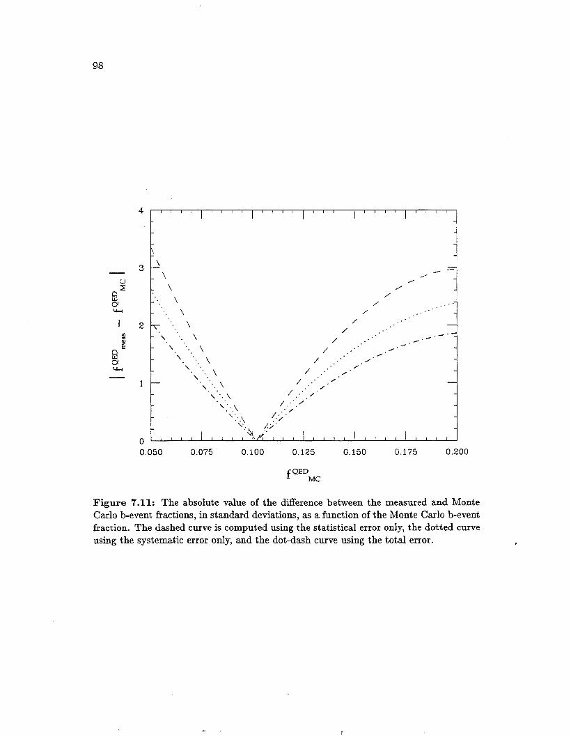
98

I v)

(Y

E

E u-c

0.050 0.075 0.100 0.125 0.150 0.175 0.200

f QEDMC

Figure 7.11: The absolute value of the difference between the measured and Monte Carlo b-event fiactions, in standard deviations, as a function of the Monte Carlo b-event fraction. The dashed curve is computed using the statistical error only, the dotted curve using the systematic error only, and the dot-dash curve using the total error.

99

sets, each set with one of the values of f $ z D used in this section. We find f::: in each of these sets, for each set using the neural network and the Monte Carlo bottom and non-bottom event-tagging network output distributions created using the same value of f $ z D . We expect f$Ef = fgzD, within statistics, for each of the five points, and this is what we find.

7.7 Discussion of the Results

This measurement of f QED = 10.2?q::?::;% = 10.2?::!% is statistically compatible with the Standard Model prediction that f Q E D = 1/11 = 9.1%. The systematic error on this measurement is somewhat larger than the statistical error.

Three large systematic errors in Table 7.3 are overestimates, since the event shape parameters were not retuned. These systematic errors are due to the uncertainties in the bottom quark mass (0.43%)) the pattern recognition efficiency (0.35%), and the nuclear interaction simulation (0.32%). The size of these three systematics could be significantly reduced by evaluating these systematic errors doing the retune, but even if all three errors turned out to be zero, the net systematic error would shrink only 25%, and the total error on f Q E D would shrink only 16%.

7.7.1 How o(fQED) Depends Upon o(f,&g:)

Each point on the best-fit parabola has a statistical uncertainty of k0.75% on f$::. Yet the average of the positive and negative statistical errors on f Q E D we report is &1.9%. This magnification of the statistical error, as well as the magnification of the systematic and total errors, is produced by the non-zero slope

We use Figure 7.12 for a geometrical derivation of this magnification factor for

Let the vertical distance between the 1-a contours be 2W, where W is the error on the ordinate of each point of the tangent. W is independent of m. The hypotenuse of the triangle in Figure 7.12 has a length equal to that portion of the diagonal in Figure 7.10 between the 1-a contours. The projection of the hypotenuse onto the horizontal axis, 2E, is twice the error on f Q E D . 2E is also the length of each leg of the triangle in Figure 7.12. Let 2E = 2W + L, then it is true that L/(2E) = tan0 = m, and 2W = 2E-L = 2E(l-m). Therefore, E = W/( l -m) , whch is the relation that we seek.

This relation is singular for m = 1, but the expression is not valid for m near 1, since this situation implies that the best-fit parabola is approximately tangent to the diagonal, and that the 1-0 contour is entirely above the diagonal. Since the 1-CT

of the parabola at the point where f::: = fMc QED .

any type of error. We approximate the parabola with its tangent at f:;: = f M c QED .

100

contour dips significantly below the diagonal in this analysis, we do not consider the case where rn is near 1. In this analysis, m = 0.60 f 0.02. For the statistical error, we predict E to be 0.75%/(1 - 0.60) = 1.9%) which is the average of the positive and negative statistical errors on this measurement. For the systematic error, we predict E to be 0.97%/(1 - 0.60) = 2.4%) which is the average of the positive and negative systematic errors on this measurement. For the total error, we predict E to be 1.23%/(1 - 0.60) = 3.1%) which is a little less than 3.2%) the average of the positive and negative total errors on this measurement; the difference is the result of the large size of the error coupled with the non-linearity of the dependence of f::: upon fMc QED .

Figure 7.12: Geometrical picture of how the error is magnified.

If the variation of fg:: as a function of fzzD is not taken into account, as has been done here, the error on fQED can be significantly underestimated. Also, the value of f::: reported can be biased if rn is large enough, and if it is significantly different, statistically speaking, horn the value of f M c QED .

7.7.2

There are three published measurements, using a neural network in a manner similar to the method used here, of the fraction of hadronic events that are bottom events. All of these are measurements of I'(Zo--. b6) at LEP [114, 115, 1161. All three fit linear combinations of histograms of the number of events as a function of the neural network output(s) for Monte Carlo events of different flavors to a histogram of the number of events as a function of the neural network output(s) for experimental data events, as described in Section 6.4.2 and References [114, 1151.

In Table 7.7, we list the results of our measurement and of the three LEP

Comparison to LEP Measurements of r(Zo+ b6)

101

measurements. The errors for our measurement is significantly larger than that on the LEP measurements.

Each of the LEP experiments has of the order of 100 times as much data as the TPC/2y experiment. Therefore, in the absence of other factors, we would expect the statistical error on our measurement to be 10 times the average of the statistical errors for the three LEP measurements. Table 7.7 shows that the difference is a factor of 4. The change from 10 to 4 is caused by the greater differences between the properties of bottom and non-bottom events at 29 GeV compared to 92 GeV,

measurement. and by the magnification of the errors by the variation off::: with f M c Q E D in this

I Experiment I Bottom event fraction I - I

+ 2 . 0 + 2 . 7 ~ TPC/2y I 10-2-1.8-2.2 0

22.2 z.t 0.3 f 0.7 % 22.8 f 0.5 z.t 0.5 % 23.2 iz 0.5 f 1.7 %

ALEPH DELPHI

Table 7.7: All measurements of the bottom event fraction using a neural network. The first error is statistical, the second systematic. Our measurement of the bottom event fraction in the continuum (first row) is expected to be very different from the bottom event fraction at the Zo (other three rows); the purpose of this table is to compare the errors on these measured fractions, not the fractions themselves.

The central feature of this measurement is the care with which the dependence of f2:, upon f $ z D was takenqnto account. There is no mention in Refer- ence [115] (Section 6.4.2) that the L3 measurement took into account the variation of r(Z0+ bb),,,, as a function of r(Z0+ b&)MC. The value of r(Z0-+ bb),,,, found by the ALEPH measurement [114] is reported to be insensitive to large changes in r(Z0-+ b b ) ~ ~ , which is surprising because of the sharp contrast with what we found in this measurement. It would be very interesting to know just how r(Zo-+ bb),,,, depends upon I'(Zo-+ ~ & ) M C , and to understand why the dependence of the measured bottom event fraction upon the Monte Carlo bottom event fraction is so different in the two measurements.

The DELPHI measurement [116] (Section 6.4.2) used a method of taking into account the variation of r(Z0-+ bb),,,, as a function of r(Zo-+ b 6 ) ~ ~ that is very different from the method used in this measurement. The DELPHI best tune was found by varying the Monte Carlo parameters to minimize the x2 of the difference between the distributions of data and Monte Carlo in rapidity and aplanarity. In the evaluation of systematic errors, the range of each Monte Carlo parameter was found by finding the extreme values of that parameter that make the x2

102

equal to XL tune + 16, allowing the values of r(2O-t b6)MC and r(ZO-1 C Z ) ~ ~ to float to minimize the x2 for a fixed value of the parameter in question. This approach magnifies the systematic error, rather than the total error, in order to take into account the variation of l ? ( Z o j b6),,,, as a function of I'(Zo+ b 6 ) ~ ~ . This approach has an understandable logic to it, and perhaps it produces results similar to the approach used in this analysis. We believe that this approach has two disadvantages compared to the approach used here:

1. The DELPHI method does not show how F(Zo--, @meas varies as a function of r(zo+ b 6 ) M c .

2. The correlations between Monte Carlo parameters were not taken into account in the DELPHI measurement, and this can lead to an underestimate of the range of the Monte Carlo parameters, which in turn will cause the systematic errors to be underestimated.

103

Chapter 8

A Study of Bias in Techniques to Measure Charged Hadron Production in Bottom Quark Jets

Up until now, neural networks have only been used in High Energy Physics, either for measurements where something is being counted, such as the number of bottom quark events in a sample, or for lower level classification problems. Both uses are described in Section 6.4.

It is highly desireable to use a neural network to do tagging measurements, especially measurements involving bottom hadrons. Measurements at LEP where identifying bottom jets with a neural network might be useful include measurements of the bottom hadron lifetime and b-mixing measurements, the latter using a network that can identify the bottom quark charge. At higher-energy colliders, tagging bottom jets is useful for identifying particles that decay predominantly into one or more bottom quarks, such as the top quark or lower-mass higgses.

In this chapter, we describe a study of bias in techniques to measure the T*, K*, and p/p (charged hadron) momentum spectra for bottom jets, using a neural network to identify the bottom jets. We begin this chapter with a description of our neural network for tagging bottom jets. We then show that bias is present in any measurement of charged hadron production in bottom jets, where a neural network tags the bottom quark jets. Finally, we describe an investigation of the sources of this bias.

104

8.1 Introduction

In any measurement technique, it is important to avoid bias as much as is practical. In some measurements, avoiding bias is impossible and a bias correction is made, but efforts are still made to design the measurement so that the bias is as small as practical. Avoiding bias is particularly important in measurements that use a neural network to tag bottom jets, since we depend heavily upon Monte Carlo to train our neural network. Avoiding bias is a factor in many of the choices made in constructing the study presented here.

One of these choices was to divide each event into two halves. The tracks in one half of the event are used for computing inputs to the neural network we use for distinguishing bottom and non-bottom events, and the tracks in the other half of the event are used to measure charged hadron production. This approach avoids using the same track to compute both the neural network inputs and the charged hadron production. To avoid bias, we also chose to use the plane perpendicular to the event thrust axis to divide the event in half, since the thrust axis tends to not have tracks close to the plane perpendicular to it [119]. We often refer to each half of an event as a jet, since we only use 2-jet events in this study (see Section 8.2), and since the tracks in each half of the event mostly come from one QCD jet.

8.2 Track and Event Selections

The track selection used in this study is the good track selection described in Section 5.2.

The event selection used are the selections described in Section 5.2, plus these additional criteria:

1. Events must be 2-jet (selected by LUCLUS with djoin = 2.5), thus eliminating obvious 3-jet events, where the gluon jet might correlate the two halves of the event and cause information to flow between the two halves of the event.

2. Events must have at least 7 charged tracks, since LUCLUS automatically classifies events with 6 or less tracks as 2-jet.

3. Events with a jet axis with dip 1x1 > 45" are cut to eliminate events with a significant number of tracks that do not enter the TPC fiducial volume. The axis of each jet is the sum of the momenta of the tracks in the jet.

4. Events where the angle between the axes of the two jets is less than 140" are cut to eliminate events with an energetic third jet that is not seen.

105

15091 events satisfy all of these selection criteria. For the tracks in the tagged jet, which are used to obtain the charged hadron

momentum spectra, we must apply selection criteria that are more restrictive than the good track selection described in Section 5.2:

1. Tracks must have a dip [ A I < 60") since the track acceptance declines with increasing dip starting near 60".

2. Tracks must have a distance of closest approach to the interaction point less than 3 cm in the x-y plane, and less than 5 cm in z, so that the track is consistent with coming from the event vertex. This criterion eliminates tracks that come from nuclear interactions or cosmic rays.

3. Either dC < 0.15 GeV-l or dC/C < 0.15, where C is the curvature, and dC is the curvature error. This ensures that the track momentum is well measured.

4. There must be at least 40 wires associated with each track, since the behavior of the dE/dz resolution is not well understood for tracks with less than 40 wires.

5. Positively charged tracks with xp = p/pb,- < 0.25 are not used, in order to exclude nuclear interaction products. The remainder of the positive tracks and all negative tracks are used in this study.

8.3 The Jet-Tagging Neural Network

Since the jet-tagging neural network's inputs contain information from only one half of each event, this network will not distinguish b from non-b as well as the event-tagging neural network described in Section 7.1. In an attempt to have good network performance, the inputs for this study's network are designed using the raw input approach described in Section 6.3.

The 15 inputs for each jet are defined as follows. A coordinate sytem is constructed as defined below, and the tracks in each jet are ordered in rapidity y (= f log [ z] , we assume the charged pion mass): track number 1 is the track with the largest y, track number 2 is the track with the second largest y, etc. Inputs 1-3 are p , , p , , and p , (respectively) for track 1, inputs 4-6 are p, , p , , and p , (respectively) for track 2, and so on for the 4 leading tracks in the jet, giving 12 inputs. Inputs 13-15 are lp,l, Ip,\, and C lp,l (respectively), where the sum is over all but the 4 leading tracks.

We define the coordinate system two ways. The simplest way, the uniteruted method, is illustrated in Figure 8.1. The z axis in each jet is defined to be parallel

106

to the thrust axis and points away from the plane that divides the event in half. The x axis is defined to be perpendicular to the event plane, which contains the thrust axis and the thrust major axis. The sign ambiguity in the choice of the perpendicular direction is handled by randomly choosing the sign. The y axis is set equal to i x 2. The x axes for the two jets are defined to point in the same direction, requiring that the y axes be in opposite directions. The coordinate systems in the two jets are fixed relative to each other, so we expect that this definition of the coordinate systems carries information between the. two halves of the event. We use this definition of the coordinate system only in our study of the bias of techniques to measure charged hadron production in bottom quark jets.

The other way we define the coordinate system, the iterated method, is designed so that the coordinate systems for the two halves of the event are relatively independent of each other. However, any method dividing the event in half must use information from the entire event, so it is impossible for the coordinate systems in the two jets to be completely independent of each other. This method is illustrated in Figure 8.2. We use the LUCLUS cluster-finder to divide each jet into two subjets. is equal to the sum of the momenta of the tracks in the subjet with the largest momentum, and & is equal to the sum of the momenta of the tracks in the other subjet. The z axis is defined to be parallel to the vector sum of the momenta of all the tracks in the jet. The z axis is 2 = (21 x i2)/lil x 2 2 1 . The y axis is defined to be $ = i x 2. In the iterated definition of the axes, the plane that divides the event in half generally does not contain the x and y axes, and the event plane generally does not contain AI and Z2.

We use the iterated definition in our study of the bias, and we would use it in a measurement of charged hadron production in bottom events. Figures 8.3 through 8.6 show the distributions of Monte Carlo bottom and non-bottom jets for the 15 inputs computed using the iterated definition of the axes. The distributions of the pz and p y inputs are asymmetric in these figures as a result of our way of defining the x and y axes. Note that many, but not all, of the inputs have different distributions for non-bottom and bottom jets. The discussion in Section 2.5 provides an explanation for the gross features of the input distributions. The p , for the four leading tracks is smaller for bottom jets than for non-bottom jets, in agreement with the observation that hadrons in bottom jets have less momentum than hadrons in non-bottom jets. p , and p , for the four leading tracks are equal for bottom and non-bottom jets, in agreement with the observation that p l is the same, for individual tracks, for non-bottom and bottom jets. However, inputs 13 and 14 are larger for bottom jets than for non-bottom jets, since bottom jets have a larger average multiplicity, and more tracks in the sum over all but four tracks, than non-bottom jets. Input 15 is larger for bottom jets than for non- bottom jets presumably because of the larger charged multiplicity for bottom jets versus non-bottom jets.

107

Thrust minor axis

x-axis

1 z-axis

major axis

+----.+ Thrust axis

/Plane that divides the

/ event in half

Figure 8.1: The uniterated coordinate system.

x-axis i y-axis

axis = 9

Figure 8.2: The iterated coordinate system. il is the sum of the momenta of the tracks in the subjet with the largest momentum, and & is the sum of the momenta of the tracks in the other subjet.

108

Figures 8.4 and 8.5 show that pz and p y for the four leading tracks have essentially identical distributions for bottom and non-bottom jets. These inputs do carry a substantial amount of information, for when these 8 inputs are eliminated and a network using the other 7 inputs is trained the same way the 15-input network is trained (described below), the network F (described in Section 6.3) declines from 0.157 to 0.109. The p , and p , inputs carry information that allows the reconstruction of the invariant masses of all subsets of the four leading tracks. In addition, a comparison of the relative spread of momenta in p , versus p , distinguishes jets in planar 3-jet events from rounder bottom events, and both from more pencil-like jets in 2-jet non-bottom events. This illustrates the ability of neural networks to distinguish the distributions of bottom and non-bottom jets from each other in the 15-dimension space of inputs, even though the projections of these distributions onto one of the inputs are sometimes identical.

A neural network with one node for each of the fifteen inputs, one hidden layer, and one output node was trained on Monte Carlo events that pass the event selections, in the same manner that the event-tagging network was trained (Section 7.2). Jets with four or fewer tracks do not have network inputs calculated, since some of the inputs would not be defined, but neither are they discarded. These low-multiplicity jets are placed in their own bin in the histograms of network outputs at y = 1.05 (and F is calculated taking into account this extra bin). Strictly speaking, these low-multiplicity jets do not possess a network output, and it is not possible for the network output to be 1.05, but we refer to these low- multiplicity jets as having a network output of 1.05.

The network was trained with a variety of number of hidden nodes, so that we could pick the number of hidden nodes at the lower end of the range in which the performance F levels off (Figure 8.7). The chosen number is 15, though 12 would have worked just as well. The number of patterns per network parameter was set to 200, as was done for the event-tagging network (Section 7.2). Figure 8.8 shows how F for the training and test sets varied as a function of the epoch number during the training. Figure 8.9 shows the network output distribution for Experiments 14-18, along with the extra bin at 1.05. Figure 8.10 shows the network output distributions for Monte Carlo bottom and non-bottom jets, along with the extra bin at J.05.

We have done a fit of a linear combination of the network output distributions for Monte Carlo bottom and non-bottom jets to the output distribution for Experiment 14-18 jets, in the same way that the fit of the bottom event fraction was done in Section 7.4.1. The fitted fraction of bottom jets is 0.0747 f 0.0079. Figure 8.11 shows the fitted linear combination of the two Monte Carlo histograms of Figure 8.10 superimposed on the experimental data histogram, along with the fitted b and non-b components. Figure 8.12 shows the bottom jet efficiency for the sample of jets above a cut on the neural network output. Also shown are the

109

0.05

0.04

0.03

0.02

0.01

0.00 0 2 4 6 8 10

pz track #1, GeV/c

0.05

0.04

0.03

0.02

0.01

0.00 0 1 2 3 4 5

pz track #3, GeV/c

0.032

0.024

0.016

0.008

0.000 0 1 2 3 4 5 6

pz track #2, GeV/c

pz track #4, GeV/c

Figure 8.3: Jet-Tagging Neural Network inputs 3 (a), 6 (b), 9 (c), and 12 (d), which are the p , for tracks 1, 2, 3, and 4, respectively. Solid is bottom, dotted is non-bottom. The area under each curve is 1.

110

0.00

0.05

0.04

0.03

0.02

0.01

0.00

,J, ;i__ '. -

0.07

0.06

0.07 i 1

- a

px track #3, GeV/c

0.07

0.06

0.05

0.04

0.03

0.02

0.01

b

px track #2, GeV/c

0.07

0.06

0.05

0.04

0.03

0.02

0.01

0.00 ....

-0.8 -0.4 0.0 0.4 0.8

px track #4, GeV/c

Figure 8.4: Jet-Tagging Neural Network inputs 1 (a), 4 (b), 7 (c), and 10 (d), which are the p z for tracks 1, 2, 3, and 4, respectively. Solid is bottom, dotted is non-bottom. The area under each curve is 1.

111

0.06

0.05

0.04

0.03

0.02

0.01

0.00 -1.2 -0.8 -0.4 0.0 0.4 0.8 1.2

py track #1, GeV/c

py track #3, GeV/c

0'040 L

1.2

py track #2, GeV/c

0'040 I 0.032

0.024

0.016

0.008

0.000 -1.2 -0.8 -0.4 0.0 0.4 0.8 1.2

py track #4, GeV/c

Figure 8.5: Jet-Tagging Neural Network inputs 2 (a), 5 (b), 8 (c), and 11 (d), which are the p , for tracks 1, 2, 3, and 4, respectively. Solid is bottom, dotted is non-bottom. The area under each curve is 1.

112

0.07

0.06

0.05

0.04

0.03

0.02

0.01

0.00 0.0 0.4 0.8 1.2 1.6 2.0 2.4

Clp,l, tracks 5+, GeV/c

0.040

0.032

0.024

0.016

0.008

0.000

r: :: 0.032

. ::L ..- . . .. .

0.024

0.016

0.008

0.000

b

0.0 0.8 1.6 2.4 3.2 4.0

Clpyl, tracks 5+, GeV/c

1; C : ..

0 1 2 3 4 5 6

CIp,I, tracks 5+, GeV/c

Figure 8.6: Jet-Tagging Neural Network inputs 13 (a), 14 (b), and 15 (c), which are IpLI, respectively. The sum is over all tracks but the leading 4.

Solid is bottom, dotted is non-bottom. The area under each curve is 1. lpzl, C IpyI, and

113

0.12

0.10

0 . 0 8 - '

purities of the samples above and below the cut. The efficiencies and purities are calculated using the fitted Monte Carlo b and non-b components of the experimental data shown in Figure 8.11. The bin at 1.05 is ignored in the computation of the efficiency and purity: it can be considered a separate sample of jets.

We apply corrections, to the fitted fraction of 0.0747 f 0.0079, for backgrounds (see Section 7.4.2), for acceptance, and for all of the physics effects discussed in Section 2.7. We find the fraction of bottom jets in qij events in QED with zero- mass quarks to be 0.0732 f 0.0078, which is 2.30 below the expected fraction of 1/11. We do not find the point where f::: = fMc , as was done in Section 7.6, and we do not compute systematic errors.

QED

- X

- -

" " " ' ' I ' " " " ' ' 1 ' -

X X

X

X X X

i

Number of Hidden Nodes

Figure 8.7: F as a function of the number of hidden nodes for the Jet-Tagging Neural Network. The arrow marks the chosen number of hidden nodes (15).

8.4 Techniques for Measuring Charged Hadron Production in Bottom Quark Jets

A conceptually simple approach was used to find the charged hadron momentum spectra for most of the previous analyses described in Section 2.6. The first step in this approach was to use a quark flavor tags to form two samples of tagged jets, each sample having a high purity of one type of quark. The remainder of the entire hadronic data set was used as a third set of jets. Then the charged hadron momentum spectra was found in each of these three samples, and each spectrum corrected for bias and acceptance. Finally, the Monte Carlo-estimated

114

0.18 Training Terminated

0.17

0.16 1 0.15

ffi

% Training IF

0.13 z"

Test F

100 300 500 700 900

Epoch Number

Figure 8.8: F as a function of epoch number for the Jet-Tagging Neural Network.

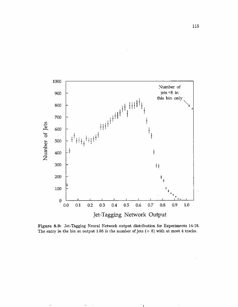
115

1000

900

800

700 rn r a, 600 0 k 500 Q) 9 E 400

300

200

100

0

*

2

Number of jets% in

this bin only

\

t t t t$t +I+ ' t

t t

t t

t t

+ + + t

0.0 0.1 0.2 0.3 0.4 0.5 0.6 0.7 0.8 0.9 1.0

Jet-Tagging Network Output

Figure 8.9: Jet-Tagging Neural Network output distribution for Experiments 14-18. The entry in the bin at output 1.05 is the number of jets (+ 8) with at most 4 tracks.

116

-

0.06

0.05

0.04

0.03

0.02

0.01

0.00 0.0 0.1 0.2 0.3 0.4 0.5 0.6 0.7 0.8 0.9 1.0


Figure 8.10: Jet-Tagging Neural Network output distributions for Monte Carlo non- bottom and bottom jets. The entries in the bin at output 1.05 are the number of jets (i 8) with at most 4 tracks. The area under each curve is 1.

117

1000

900

800

700 m a, 600 u-c 0 k 500

$ 400

300

200

100

0

-la

2 z

Number of jets e8 in this bin only

Non-Bottom

Non- Bottom

B plus

jnn-B

i Bottom h

f I I I I I I u- - 0.0 0.1 0.2 0.3 0.4 0.5 0.6 0.7 0.8 0.9 1.0


Figure 8.11: The fitted jet-tagging neural network output distributions for Monte Carlo b and non-b jets, their sum, and the output distribution for Experiment 14-18 jets. The entries in the bin at output 1.05 are the number of jets (+ 8) with at most 4 tracks.

.

118

0.9

0.8

0.7

0.6

0.5

0.4

0.3

0.2

-

-

-

-

-

-

-

-

0.1

0.0

Jet B JetPurity Below Cut Above cut 1.

I I I I I I I

_ -

0 .O 0.2 0.4 0.6 0.8

Jet-Tagging ‘Network Output

Figure 8.12: Bottom jet efficiency for the sample of jets with network output above the cut on the abscissa. Also shown are the purities of the samples above and below the cut. The bin at output 1.05 is ignored in the computation of the efficiency and purity.

119

quark content of these three samples was used to extract, from the momentum spectra of these samples, the charged hadron momentum spectra for bottom jets, for charm jets, and for light-quark jets.

This approach is ideal for the tagging methods described in Section 2.6 because each of these tags produce one sample of tagged jets, each sample highly enriched in one quark type. In contrast, a neural network output offers no obvious samples, and Figure 8.12 shows that the sample of jets above any cut on the network output does not have a high bottom jet purity.

We attempted to develop a likelihood function to extract the hadron momentum spectra. There are two motivations for taking this approach. The first motivation is that using two cuts on the neural network output to divide the tagged jets into three samples throws away information present in the distribution of network outputs1, whereas a likelihood fit does not throw away this information. The second motivation is that a likelihood fit makes use of the information in the differences between the hadron momentum spectra in fitting the quark fractions and hadron momentum spectra, whereas extracting the hadron momentum spectra from three samples of tagged jets only uses the quark contents of the three samples.

One disadvantage of using a likelihood function is that it requires a model for track-track correlations in the tagged jet. We made the approximation that there are no track-track correlations, and we excluded positively charged tracks from the hadron momentum spectra to remove short-range’ charge and flavor correlations (Bose-Einstein correlations are not removed). This assumption and selection were inadequate, resulting in bias of the fitted hadron momentum spectra in a fit to a Monte Carlo sample. The other disadvantage of using a likelihood function is that bias and acceptance corrections can only made on the fitted hadron momentum spectra, not on the input to the fit. In contrast, it is simple to apply bias and acceptance corrections to the hadron momentum spectra for the three samples before the extraction of the hadron momentum spectra for the different types of quark jets.

We do not pursue the alternative approach of using two cuts on’the neural network output to divide the tagged jets into three samples, though there is no reason it can not be done.

‘This can be seen by coarsening the binning in Figure 8.10 so that there are only three bins. 2Short-range in rapidity.

120

8.5 A Test for Bias in Measurements of Charged Hadron Production in Bottom Quark Jets

In this section, we test for bias in techniques to measure charged hadron production in bottom quark jets by determining if the hadron momentum spectra in Monte Carlo for the tagged jet is independent of the value of the jet-tagging neural network output for the tagging jet. Our test of independence works as follows. We divide the range of the neural network output from 0.0 to 1.0 into 10 bins with width 0.1, place the jets with network output 1.05 into an eleventh bin, and compute the hadron momentum spectra in each of these 11 bins separately for the tracks in bottom, charm, and light-quark (up, down, and strange) Monte Carlo tagged jets that pass all the selections described in Section 8.2. For pions, we use 12 bins in momentum with boundaries .006, .015, .030, -045, .060, -075, .090, -12, .15, 2, .3, . 5 , and .9 in the scaled momentum xp = p/pb,,. For kaons and protons, we use 4 bins in momentum (because fewer of these particles are produced) with boundaries .006, .045, .090, .2, and .9 in xp.

For this test, we use 49096 light-quark, 35592 charm, and 74800 bottom jets that pass the selections described in Section 8.2 (Approximately 6.3, 6.3, and 46, respectively, times the number of jets in the Experiment 14-18 data set that pass the same selections.). Once we obtain the hadron momentum spectra in each of the 11 network output bins, we scale the spectra so that each network output bin contains the same total number of hadrons. Finally, we compute the confidence level, in each momentum bin, for the scaled cross-section to be the same in all 11 bins in the neural network output. We compute this confidence level separately for each of the three types of quarks and for each hadron.

We show these confidence levels in Figures 8.13 through 8.15, with light-quark and charm-quark jets separate and combined. The confidence levels for the pion spectra are essentially zero in some momentum bins. The confidence levels for the kaon and proton spectra are larger than for the pion spectra because fewer kaons and protons are produced, but in some momentum bins these kaon and proton confidence levels are about 1% or less. The hadron momentum spectra in the tagged jet obviously depend upon the network output of the tagging jet. Unless there is a miraculous cancellation ih the contribution of this dependence to the bottom-jet hadron momentum spectra in each momentum bin, these spectra will be biased3. The statement that the spectra are biased applies to any technique of measuring charged hadron production in bottom quark jets that uses our neural network to tag the bottom jets. Since we have taken pains to define the neural

3That the confidence levels in Figures 8.13d, 8.14d, and 8.15d, with charm and light-quark jets combined, are sometimes far smaller than the confidence levels for charm and light-quark jets treated separately confirms that the hadron momentum spectra should be found separately for charm-quark and light-quark jets.

121

network inputs so that bias is minimized, any technique using any neural network will be biased.

There are two ways of correcting for this bias. The simplest way is to make bias corrections. The other way is to try to modify the technique so that the bias corrections are smaller (or so that the confidence levels in Figures 8.13 through 8.15 are closer to l), and then make the necessary bias corrections.

One possible way of modifying the technique to reduce bias is to exclude the jets with network output 1.05 from the hadron momentum spectra. When these jets are excluded, Figures 8.13 through 8.15 show that the confidence levels for the momentum spectra being independent of the network output improve, in some momentum bins, far beyond the amount expected from the decrease in the statistics. The fact that the improvement mostly takes place in the highest momentum bins of the uds-quark histograms (Figures 8.13a, 8.14a, and 8.15a), where improvement always occurs, suggests that the improvement is produced by the long-range correlation due to the common flavor of the leading quark in each jet.

In the next section, we present a systematic investigation of the possible sources of bias in techniques of measuring charged hadron production in bottom quark jets.

8.6 An Investigation of the Sources of Bias

In Section 8.5, we demonstrated that the hadron momentum spectra of the tagged jets depend upon the network output of the tagging jet. In this section, we present our investigation of the causes of this dependence.

8.6.1 Using Correlations Between Jets in Each Event to Measure Bias

We need an easy-to-compute measure of bias for our investigation of the sources of bias. The easiest, albeit indirect, way to determine how much bias there is for one quark flavor is to see if the neural network inputs in the 2 jets in each event are statistically independent, since this does not require that a neural network be trained. The advantage of this approach is that the inputs can be treated separately, and their behavior compared. This method does not provide an absolute measure of bias.

A necessary, but not sufficient, condition for two variables to be statistically independent is for the correlation to be statistically consistent with being zero. Therefore, we compute the correlation coefficient [120] of the same neural network input in the two jets. In the statistical literature, there are more sophisticated measures of independence than the correlation coefficient, but it is not necessary to use them here.

122

r - .

I I I I

- 1

2 4 6 8 1 0 1 2 2 4 6 8 1 0 1 2

Momentum Bin

r

Momentum Bin

l l

I I I I I I I I I I I I -

2 4 6 8 1 0 1 2 2 4 6 8 1 0 1 2

Momentum Bin Momentum Bin

Figure 8.13: The bin-by-bin confidence levels for the scaled pion cross-section to be independent of the network output for Monte Carlo uds-jets (a ) , charm jets (b), bottom jets (c), and udsc-jets (d). The empty-looking bins really have entries below The solid histogram includes jets with network output 1.05, the dashed histogram excludes jets with network output 1.05.

123

W z 8 5 3 5

c3

U

4 W z

1 2 3 4

Momentum Bin

10'

lo-*

1 2 3 4

Momentum Bin

- - - - - - I 10" I I

1 2 3 4

Momentum Bin

Figure 8.14: The bin-by-bin confidence levels for the scaled kaon cross-section to be independent of the network output for Monte Carlo uds-jets (a), charm jets (b), bottom jets (c), and udsc-jets (d). The solid histogram includes jets with network output 1.05, the dashed histogram excludes jets with network output 1.05.

124

1

IO'

102

16'

t 1 2 3 4

Momentum Bin 1 2 3 4

Momentum Bin

10" " I ' ' ' " I ' ' I '

1 2 3 4

Momentum Bin

1 2 3 4

Momentum Bin

' Figure 8.15: The bin-by-bin confidence levels for the scaled proton cross-section to be independent of the network output for Monte Carlo uds-jets (a), charm jets (b), bottom jets (c), and udsc-jets (d). The solid histogram includes jets with network output 1.05, the dashed histogram excludes jets with network output 1.05.

125

The common quark flavor of the two jets, in combination with the differing neural network input distributions for different quark flavors, will introduce a correlation. This is illustrated in Figure 8.16, where three circular (and therefore independent) distributions in y as a function of x are superposed; the sum of the three distributions has a positive correlation in y as a function of x, since the average of y is a function of x. We are only interested in the correlation due to information other than quark flavor crossing the boundary between the two jets, so we compute separately the correlations for uds, charm, and bottom.

X

Figure 8.16: Each of the three independent distributions (circles) is independent, but the sum of the distributions is not independent in y as a function of x.

We now have a profusion of correlation coefficients p. For the p , inputs, we have 3 flavors x 5 inputs = 15 correlation coefficients. We have the same number of coefficients for p , , p , , and y. We deal with this by combining this information into three numbers for p,, three for p, , three for p , , and three for y:

1. We average p over the 3 quark flavors and the 4 leading tracks (12 terms in the average). We also compute the standard deviation of this average.

2. We compute a x2 that the same 12 p’s (12 degrees of freedom) are all consistent ;with being zero: x2 = E( -&)2. We also compute the corresponding confidence level.

3. We need some function of only the p’s to quantify their spread, so we compute lpl for the same 12 p’s.

We use these three quantities to measure how much correlation there is. All of these quantities are computed assuming that the correlations for different tracks in the same jet are uncorrelated with each other. This assumption is not necessarily true, it is certainly not true for y when we order the tracks in y.

126

We order the tracks in y, therefore the x2 C.L. for y is unreliable for deciding whether a correlation exists in y, and we do not consider y correlated unless the x2 C.L. is less than 0.5% and unless (E IpI)/u(C p ) and p / c ( p ) are both larger than roughly 3. For p,, p , , and p, , we use the same criteria in order to be conservative.

These criteria are admittedly somewhat arbitrary, but this is not important, since many effects clearly produce large correlations.

Our first task in investigating the sources of correlations is to enumerate all possible sources of correlations, which we do in the next section. After that, we remove all of these correlations from the Monte Carlo and verify that there is no remaining correlation. We then evaluate the correlation that results when each potential source of correlations is present alone (with the other potential sources not present) in the Monte Carlo.

8.6.2 All Possible Sources of Correlations

1. Initial state radiation (ISR)

2. Gluon radiation. All events consist of back-to-back qtj pairs in the absence of ISR and gluon radiation.

3. Fkagmentation/4-momentum-conservation. In order to shut off correlations due to fragmentation, we use independent fragmentation in place of the usual string fragmentation. There are numerous 4-momentum- conservation schemes for independent fragmentation, and we have pur- posely chosen none of them, so that energy-momentum conservation does not induce correlations. As a result, the total 4-momentum is not conserved, and the total event energy has a mean of 29.0 GeV and a sigma of about 0.6 GeV.

4. All detector effects can introduce correlations, since they are dip-angle dependent and the two jets have a similar dip. Therefore, we have turned off all processes that occur in the material of the TPC/2y experiment: dE/dz energy loss, bremsstrahlung, pair conversion, and nuclear interactions. Some tracks enter the TPC volume more than once, since their paths curl up in the TPC magnetic field, so we ignore all but the first passage of these tracks through the TPC volume.

5. Using a measured quantity, such as the thrust axis, to define a plane for dividing events in half will introduce correlations, since the finding of any such axis uses information from the entire event. Instead, we use the quark axis, which is the quark’s direction. We also need a direction perpendicular to the quark axis: we pick a perpendicular direction randomly.

127

6 . We remove all particles that go into the half of the event opposite to the parton it originated from. Only in independent fragmentation can one say unambiguously which parton a hadron originated from.

7. It is common to label as jet number 1 the jet with the largest value of some quantity, such as I CpzI, the z-direction being the direction parallel to the quark axis. The other jet is jet number 2, and so the correlation of jet 1 with jet 2 is evaluated. This ordering introduces a correlation. In an actual measurement, we would randomly assign the label jet 1. If we use the quark axis, jet 1 is the quark jet and jet 2 is the antiquark jet.

8. AlI event selections are capable of creating correlations:

(a) The Good Hadronic Event Selection.

(b) The 7-27 event selection.

(c) The selection of only %jet events.

(d) The cut on the angle between the axes for the two jets in each event.

(e) All cuts on particle momentum, dip, etc.

(f) All cuts on event axis dip angle.

8.6.3 Which Sources of Correlation Contribute

In our investigation of the sources of correlation, 120k Monte Carlo events are used (except as stated), whereas the good hadron DSTs for experiments 14-18 contain about 39k events.

8.6.3.1 The Baseline for this Investigation

To start with, we need to compute the measures of correlation in the neural network inputs, with all possible sources of correlations removed, as a baseline against which to compare all variations in the Monte Carlo and in the computing of the network inputs. We do this in the first row of Table 8.1.

Row number two of Table 8.1 shows that, at the level of statistical significance being explored here, introducing backwards-moving tracks does not produce correlations. Removing backwards-moving particles is clearly impossible to do in experimental data, and it is sometimes unwise to do so, as described in Sections 8.6.3.4 and 8.6.3.5. Therefore, in evaluating all correlations, we use backwards-moving particles, and we use the second row of Table 8.1 as the baseline against which we compare all variations of the Monte Carlo and in the computing of the network inputs. We call it “Baseline 1”. We have also evaluated (but do not show) the other

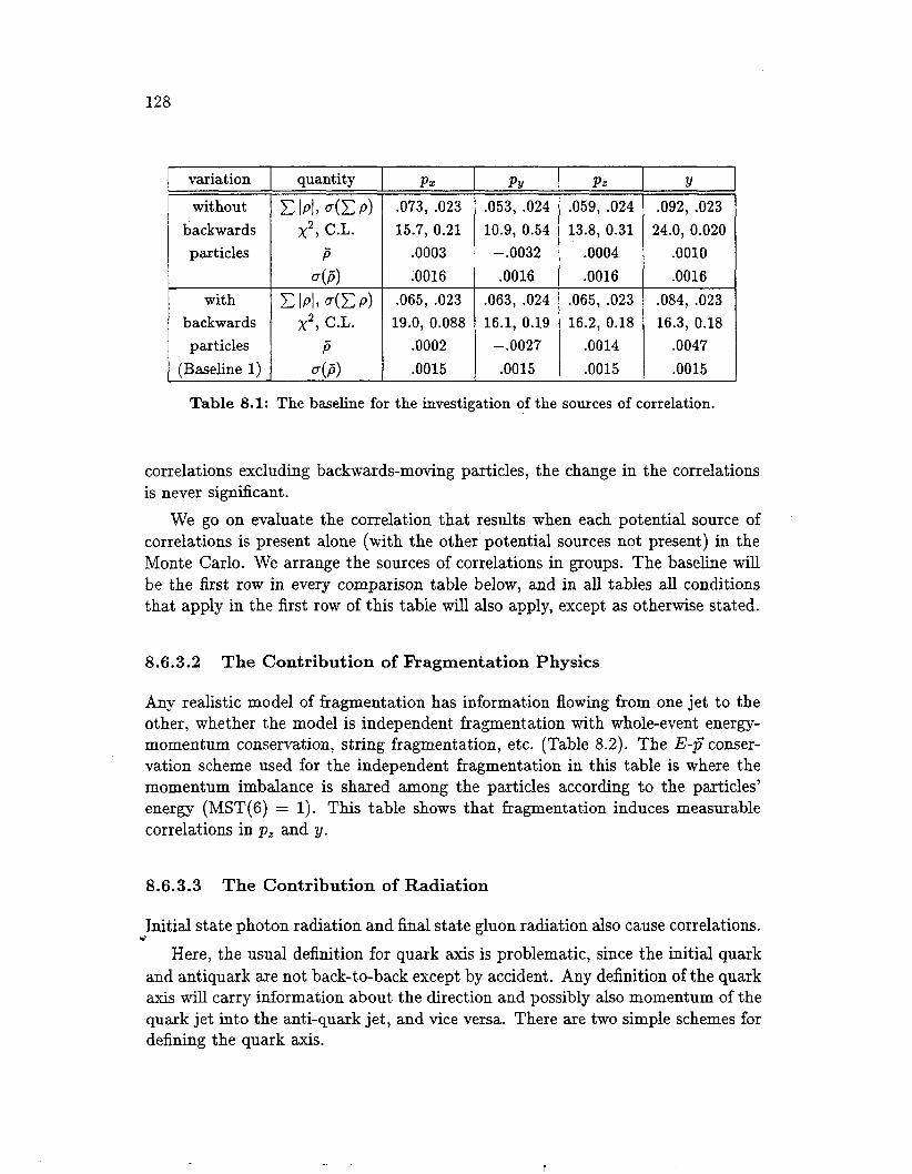
128

quantity

c IPI, 4 2 PI x2, C.L.

r? u(a>

c lPl, 4CP) x2, C.L.

P 4ij>

1 variation

backwards particles

backwards particles

Pz

*073, -023 15.7, 0.21

.0003

.0016 e0657 -023

19.0, 0.088 .0002 -0015

Pz

.059, .024 13.8, 0.31

.0004

.0016 .065, .023 16.2, 0.18

.0014

.0015

PY .053, .024 10.9, 0.54

.0016 - .0032

Y .092, .023

24.0, 0.020 .0010 -0016

.084, .023 16.3, 0.18

.0047

.0015

.063, .024 16.1, 0.19

.0015 - .002?

Table 8.1: The baseline for the investigation of the sources of correlation.

correlations excluding backwards-moving particles, the change in the correlations is never significant.

We go on evaluate the correlation that results when each potential source of correlations is present alone (with the other potential sources not present) in the Monte Carlo. We arrange the sources of correlations in groups. The baseline will be the first row in every comparison table below, and in all tables all conditions that apply in the first row of this table will also apply, except as otherwise stated.

8.6.3.2 The Contribution of Fragmentation Physics

Any realistic model of fragmentation has information flowing from one jet to the other, whether the model is independent fragmentation with whole-event energy- momentum conservation, string fragmentation, etc. (Table 8.2). The E-@ conservation scheme used for the independent fragmentation in this table is where the momentum imbalance is shared among the particles according to the particles’ energy (MST(6) = 1). This table shows that fragmentation induces measurable correlations in p z and y.

8.6.3.3 The Contribution of Radiation

Initial state photon radiation and final state gluon radiation also cause correlations.

Here, the usual definition for quark axis is problematic, since the initial quark and antiquark are not back-to-back except by accident. Any definition of the quark axis will carry information about the direction and possibly also momentum of the quark jet into the anti-quark jet, and vice versa. There are two simpIe schemes for defining the quark axis.

*’

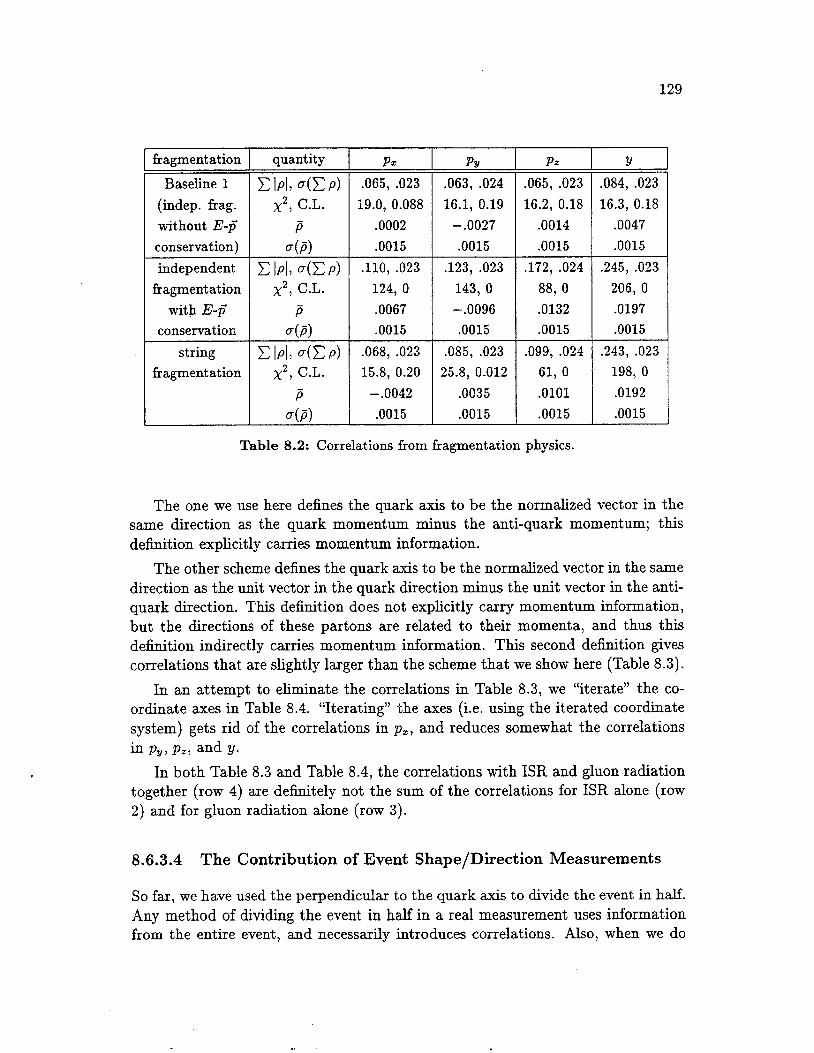
129

Pz

.065, .023 19.0, 0.088

.0002

.0015 .110, .023

124, 0 .0067 .0015

I fragmentation Baseline 1

(indep. hag.

conservation) independent

fragmentation with E-@

conservation string

fragment ation

without E-@

PY P z .063, .024 .065, -023 16.1, 0.19 16.2, 0.18

-.0027 .0014 .0015 .0015

.123, .023 .172, .024 143, 0 88, 0 - .0096 .0132 .0015 -0015

quantity

.068, .023 15.8, 0.20

-.0042 .0015

.085, -023 .099, .024 25.8, 0.012 61, 0

.0035 .0101

.0015 .0015

Table 8.2: Correlations from fragmentation physics.

Y .084, .023 16.3, 0.18

.0047

.0015 .245, .023

206, 0 .0197 .0015

.243, .023 198, 0 .0192 .0015

The one we use here defines the quark axis to be the normalized vector in the same direction as the quark momentum minus the anti-quark momentum; this definition explicitly carries momentum information.

The other scheme defines the quark axis to be the normalized vector in the same direction as the unit vector in the quark direction minus the unit vector in the antiquark direction. This definition does not explicitly carry momentum information, but the directions of these partons are related to their momenta, and thus this definition indirectly carries momentum information. This second definition gives correlations that are slightly larger than the scheme that we show here (Table 8.3).

In an attempt to eliminate the correlations in Table 8.3, we “iterate” the coordinate axes in Table 8.4. “Iterating” the axes (Le. using the iterated coordinate system) gets rid of the correlations in p, , and reduces somewhat the correlations

In both Table 8.3 and Table 8.4, the correlations with ISR and gluon radiation together (row 4) are definitely not the sum of the correlations for ISR alone (row 2) and for gluon radiation alone (row 3).

in P, , P,, and Y.

8.6.3.4 The Contribution of Event S hape/Direct ion Measurements

So far, we have used the perpendicular to the quark axis to divide the event in half. Any method of dividing the event in half in a real measurement uses information from the entire event, and necessarily introduces correlations. Also, when we do

“. .

130

.395, .024 898, 0 .0389 .0016

radiation

4.731, .025 119901, 0

.4679

.0014

Baseline 1

radiation) (no

.659, .023 2480, 0 .0581 -0015

.620, .024 1887, 0 .0561 .0015

ISR

3.926, .023 77704, 0

.3614 -0013

4.776, .022 121494, 0

.4295

.0013

parton showers

ISR and parton showers

Px .065, .023 19.0, 0.088

.0002

.0015 .046, .025 6.4, 0.90

.0016 - .0007

.155, .024 117, 0

-0015 - .On7

.151, .025 123, 0 -.0138 .0016

PY .063, .024 16.1, 0.19

-.0027 -0015

.456, .030 997, 0 .0551 .0020

.222, .026 178, 0 -.0171 .0019

.414, .026 779, 0 .0429 .0016

.0047 .0015 .0015

Table 8.3: Correlations due to ISR and gluon radiation.

131

ISR lpl, a(Cp) .060, .024 x2, C.L. 11.9, 0.45

P .0014 4 3 .0015

parton lpl, a ( C p ) .051, .023 showers x2, C.L. 14.2, 0.29

P -.0001 .0015

ISR and / p i , a(Cp) .044, .024 parton x2, C.L. 6.8 , 0.87

showers P -.0007 .0015

i a ( d

radiation I quantity

x2, C.L. radiation) - .0012

.0015 .472, .023

1219, 0 .0087 .0015

1.298, -022 6343, 0 .1003 .0013

.060, .023 .062, .023 .072, .023 10.9, 0.54 12.7, 0.39 13.3, 0.35

.0010 .0025 .0043 i .0015 .0015 .0015

.420, .023 759, 0 .0360 .0015

.372, .023 568, 0 .0221 ,0014

.120, .019 804, 0 -.0192 .0009

1.861, .023 11373, 0

.1523

.0014 1.483, .023

5960, 0 .1000 .0014

.154, .023 129, 0 .0134 .0015

.163, .021 617, 0 -.0130 .0011

Table 8.4: Correlations due to ISR and gluon radiation, axes “iterated”.

.. .

not “iterate”, we use event the axis to define the coordinate system with respect to which we compute the neural network inputs, and this also introduces correlations (Table 8.5). This is one occasion where removing backwards moving particles is unwise, since doing so would alter the thrust axis direction.

Using a thrust axis that is computed from all of the final-state particles generated by the Monte Carlo definitely induces correlations in p , and p , that can be erased by iterating the axes. Correlations from using a thrust axis that is computed from the tracks simulated in TPCLUND as recorded by the TPC are much larger, and they can not be entirely erased in p , and y by iterating.

One must be careful that in using an algorithm that finds the thrust axis, the jets in an event are not ordered by any kinematic criteria, because this ordering will induce correlations.

8.6.3.5 The Contribution of Detector Acceptance

Detector acceptance results in loss of tracks out the ends of the detector. This will cause the observed characteristics of a jet to vary with the dip of the jet, resulting in correlations (Table 8.6).

In Table 8.6, the quark axis is always used. This is another occasion where removing backwards moving particles is unwise, since the acceptance for backwards tracks is not the same as it is for forwards tracks. We have turned off the simulation of interactions in the TPC.

In Table 8.6, the “standard dip and p cuts” are:

1. Track dip 1x1 < 60”

2. Dip of the event sphericity axis 1x1 < 45”.

3. For tracks in the track block, the momentum extrapolated to the event vertex must be at least 120 MeV/c, and the momentum in the TPC must be at least 100 MeV/c. For particles in the Monte Carlo block, we require p > 120 MeV/c.

Re-entries of tracks into the TPC do not induce correlations (row 2). Limi$ing ourselves to charged particles in computing the network inputs, in conjunction with not cutting backwards tracks, does induce y-correlations (row 3).

]Furthermore, rows 4 and 6 are compatible with being identical, thus correlations from using tracks from the track block that enter the TPC fiducial volume are reproduced by the charged tracks in the Monte Carlo block that pass the dip and p cuts.

The large y correlation in row 5 probably comes from the edges of the TPC’s fiducial volume, where the event acceptance as a function of the dip of the event

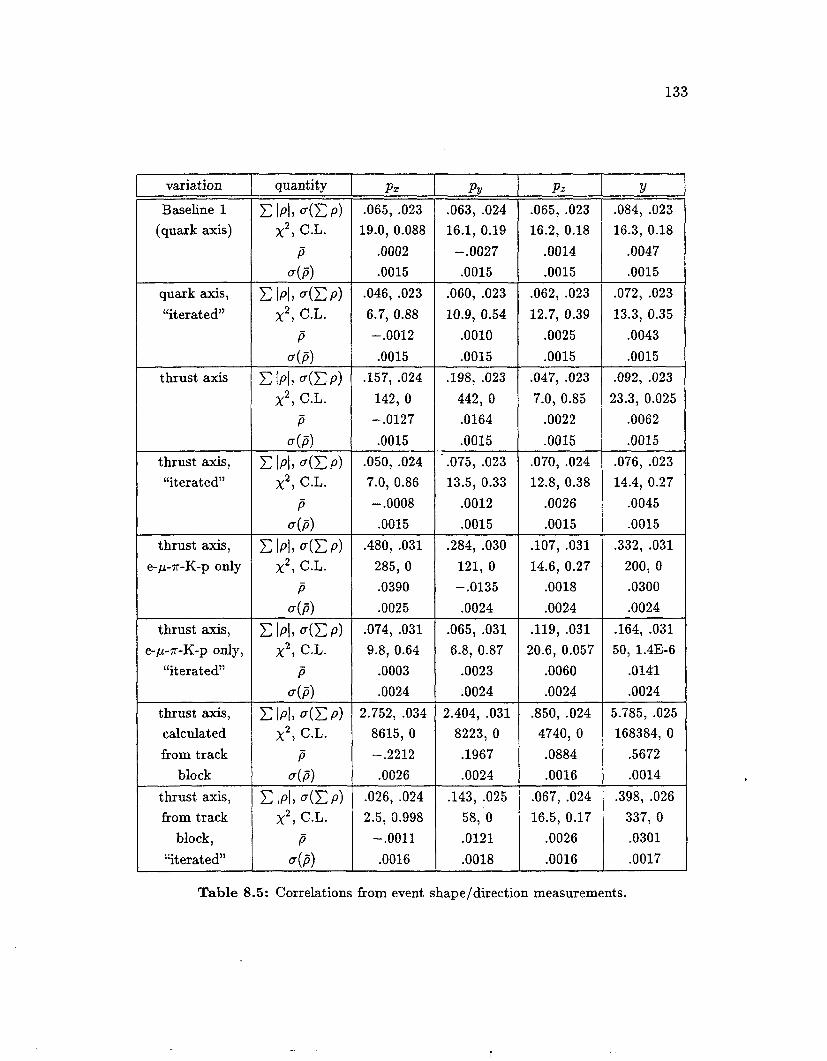
133

p , .063, .024 16.1, 0.19

-.0027 .0015

.060, .023 10.9, 0.54

.0010

.0015 .198, .023

442, 0 .0164 .0015

.075, .023 13.5, 0.33

.0012

.0015

variation P Z

.065, .023 16.2, 0.18

.0014

.0015 .062, .023 12.7, 0.39

.0025

.0015 .047, .023 7.0, 0.85

-0022 .0015

.070, .024 12.8, 0.38

.0026 ,0015

.284, .030 121, 0 -.0135 ,0024

.107, .031 14.6, 0.27

.0018

.0024 .065, .031 6.8, 0.87

.0023

.0024

.119, .031 20.6, 0.057

.0060

.0024 2.404, -031

8223, 0 .1967 .0024

.143, .025 58, 0 .0121 .0018

.850, ,024 4740, 0 .0884 .0016

.067, .024 16.5, 0.17

,0026 .0016

P X

.065, .023 19.8, 0.088

.0002

.0015

Y .084, .023 16.3, 0.18

.0047

.0015

Baseline P (quark axis)

quark axis, “iterated”

.046, .023 6.7, 0.88 -.0012 .0015

.072, .023 13.3, 0.35

.0043

.0015 thrust axis .P57, .024

142, 0

.0015 -.0127

.092, .023 23.3, 0.025

.0062

.0015 thrust axis, “iterated”

.050, .024 7.0, 0.86 -.0008 .0015

.076, .023 14.4, 0.27

.0045

.0015 thrust axis,

e-p-7r-K-p only .480, .031

285, 0 .0390 .0025

.332, .031 200, 0 -0300 .0024

thrust axis, e-p-n--K-p only,

“iterated”

.164, .031 50, 1.4E-6 .0141 .0024

.074, .031 9.8, 0.64

.0003

.0024 2.752, .034

8615, 0 -.2212 .0026

.026, .024 2.5, 0.998

-.0011 .0016

thrust axis, calculated from track

block

5.785, .025 168384, 0

.5672

.0014 thrust axis, from track

block, “iterated”

.398, .026 337, 0 .0301 .0017

Table 8.5: Correlations from event shape/direction measurements.

134

quantity


P 43

2 2 , C.L. P

4 P > c IPI, 4 C PI

2 2 , C.L. P

4 P ) c IPI, 4 C P>

x2, C.L.

di3

c lPl, 4CP)

P

variation P X

-065, -023 19.0, 0.088

.0002

.0015 -066, -023 14.9, 0.25

.0002

.0015 -052, -030 4.7, 0.967

.0009

.0024 J96, -039 10.1, 0.61

.0031 -.8017

Baseline 1 (Monte Carlo

block, all particles)

MC block, all particles plus

tracks that re-enter TPC Monte Carlo

block, e-p-T-K-p only

P Z

.065, -023 16.2, 0.18

.0014

.0015 .065, .023 16.4, 0.17

.0013

.0015 .093, .031 11.0, 0.53

.0044

.0024 -134, .041 14.3, 0.28

.0083

.0031

MC block, e-p-7r-K-p only,

standard dip and p cuts

Y .084, .023 16.3, 0.18

.0047

.0015 .083, .023 15.5, 0.21

.0046

.0015 .143, .031

40, 0.00006 .0126 .0024

.170, .040 34.8, 0.0005

.0111

.0031 track block c IPI, 4CP)

x2, C.L.

d b ) P

track block, standard dip and p cuts

-142, -034 26.2, 0.010

.0026 -.0106

.162, ,032 38, 0.00014

.0065

.0019

.776, ,037 470, 0 .0605 .0030

c lPl, 4 C P> -090, SO38 x2, C.L. 12.7, 0.39 i 4 P ) .0027

-.0012

PY

.063, .024 16.1, 0.19

-.0027 .0015

.049, .024 11.9, 0.45

-.0026 .0015

.log, .031 18.3, 0.11

.0029

.0024 .128, .040 12.8, 0.39

.0013

.0031 .087, .033 10.0, 0.61

-0007 .0023

.138, .040 17.3, 0.14

,0029 -.0018

Table 8.6: Correlations due to detector acceptance.

135

sphericity axis drops off quickly, the track acceptance in p is a function of dip and p , and the track acceptance in dip also is a function of dip and p .

8.6.3.6 The Contribution of Event Selections

In any analysis, various selections must be made to eliminate backgrounds to the desired process QQ 3 hadrons, and to ensure that the bulk of the event enters the fiducial volume of the detector. Any cut that is made on a quantity defined by the entire event, such as charged energy, will introduce correlations (Table 8.7).

One might consider replacing a cut on an event-defined quantity with a cut on each of the event’s two jets, for example on the minimum of the total charged energies of the two jets, but the process of dividing the event in half might introduce correlations through the cut, though the correlations might be drastically reduced by using this alternative.

However, altering the selections is not necessary. The x2 C.L. indicates that the 2-jet event selection and the jet-jet angle cut induce small correlations. The 7.-27 event selection numbers look interesting, but meet none of the criteria we use for deciding that there are significant correlations. With all selections combined, there is no evidence for correlations.

8.6.3.7 The Contribution of Interactions in Detector Material

Interactions with the material of the TPCI2-y detector are dip dependent. Tracks will be ranged out in the material in front of the TPC, multiple scattering will alter track direction, energy loss will change track momentum, and conversions, nuclear interactions, conversions, and bremsstrahlung (in conjunction with conversions) will add tracks to events. This will cause the observed characteristics of a jet to vary with the dip of the jet, causing the correlations in Table 8.8.

Conversions, nuclear interactions, and bremsstrahlung each satisfy 2 of the 3 criteria for deciding there are significant correlations in y, so we consider these to be borderline cases. dE/dz energy loss definitely causes correlations in y, as does the combination of all interactions.

8.6.4 The Relative Importance of the Sources of Corre- lation

We now compare the size of correlations. The numbers in these tables indicate that the following effects are the sources of correlations, ranked in IpI from largest to smallest:

1. ISR and gluon radiation.

136

quantity

lpl, o(C p ) x2, C.L.

5, 44

selections P x PY Pz Y .065, .023 ,063, .024 .065, .023 .084, .023

19.0, 0.088 16.1, 0.19 16.2, 0.18 16.3, 0.18 .0002 -.0027 .0014 .0047 .0015 .0015 .0015 .0015

Baseline 1

selections) (no

/pi, a(C p) x2, C.L.

5, 4i4

lpl, o(C p ) x2, C.L.

P .(A

IpI, o(C p ) x=, C.L.

P 4 4

lpI, a(Cp) x2, C.L.

ij 43

Ip ( , o(x p ) x2, C.L.

P 4 d

IpI, a(C p ) x2, C.L.

P 4)

The r-2y event

selection The Good Hadronic

Event Select ion

2-jet event selection

,090, .028 .057, .029 .097, .028 .091,.028 17.9, 0.12 6.8, 0.87 27.0, 0.0077 16.2, 0.18

.0029 - .0022 -.0058 .0006 -0021 .0021 .0021 .0021

.073, .026 .069, .027 .075, .027 .076, .026 13.4, 0.34 12.3, 0.42 17.0, 0.15 12.2, 0.43

.0015 -.0026 -.0021 .0017

.0019 .8019 ,0019 .0018 .052, .025 .052, .026 .093, .026 .086, .025 9.1, 0.70 9.1, 0.69 41.5, 0.00004 16.5, 0.17

.0021 -.0013 -.0049 -.0001

.0018 ,0018 .0018 .0018 .088, -044 .1P4, -041 .093, .041 .208, .040 6.7, 0.87 10.0, 0.61 8.9, 0.71 40.6, 0.00006 -.0018 -.0033 .0040 .0191 -0034 .0032 -0032 .0033

.104, -044 .098, -045 .108, .045 SO8, .044 9.4, 0.67 6.0, 0.92 10.2, 0.59 10.7, 0.55

.0016 -.0016 .0017 .0056

.0035 AI036 .0036 .0035 .092, .047 -132, .044 .154, .046 .148, .044 6.8, 0.87 ’11.1, 0.52 17.6, 0.13 14.6, 0.26 -.0009 -.0025 .0038 -0037 ,0037 .0036 .0036 .0036

“it era t ed” axes, cut on jet-jet

angle

cut of [dip1 < 60” for

sphericity, jet axes

all selections together

1

137

J p ] , a(c p ) x2, C.L.

ii 4 P )

lpl, a(c p ) x2, C.L.

ii a(al

interactions

Baseline 1 (no

interactions)

.056, -023 -059, .023 .073, .023 10.8, 0.54 14.9, 0.25 20.1, 0.066

-.0021 -.0017 .0017 .0015 .0015 .0015

-048, .023 -053, -023 .080, .023 7.4, 0.83 9.1, 0.69 17.0, 0.15 -.0017 -.0010 .0021 .0015 .0015 .0015

conversions

Ip(, a(C p ) x 2 , C.L.

P 4 P )

Ip1, a(Cp) x2, C.L.

zi

a(C p ) x2, C.L.

P

nuclear interactions

.052, .023 .069, .023 .041, .023 6.6, 0.88 20.4, 0.060 6.4, 0.89

.oooo .0023 .0010

.0015 .0015 .0015 .081, .023 .064, .023 .053, .023 16.8, 0.16 15.7, 0.21 13.2, 0.36 - .0008 -.0001 .0025 .0015 .0015 .0015

.054, .020 .067, .020 .063, .020 16.8, 0.16 16.6, 0.16 20.0, 0.067

-.0004 .0022 -0024 .0013 .0013 .0013

bremsstrahlung

multiple scattering

dE/dx energy loss

all interactions turned on

(179k events)

.0002 -.0027 -0014

.0015 .0015 849, .023 .048, -023 .070, ,023 5.4, 0.94 7.6, 0.82 12.7, 0.39 -.0006 - .0005 .0016 .0015 .0015 .0015

Y .084, .023 16.3, 0.18

.0047

.0015 .086, .024

36.4, 0.00028 .0031 .0015

.084, .024 33.7, 0.00074

.0029

.0015 .081, .024

29.5, 0.0033 .0023 .0015

.056, .023 8.6, 0.74

.0020

.0015 .079, .023

39.8, 0.00008 .0063 .0015

.085, .020 38.7, 0.0001

.0059

.0013

Table 8.8: Correlations caused by interactions in the detector material.

1

138

2. Use of the thrust axis, when only charged tracks are used.

3. Ragmentation physics.

4. Detector acceptance, the jet-jet angle event cut.

5. The 2-jet event selection.

6. dE/dz energy loss, conversions, nuclear interactions, and bremsstrahlung.

Note that the first and third largest sources of correlations are from physics, not from the method used to compute the network inputs, and can not be eliminated. The second-largest source is from the method used to compute the network inputs, but this source can not be eliminated since events must be divided in half.

Factors that do not measurably contribute are:

1. The other event selections:. the Good Hadronic Event Selection, the 7-27 selection, and the cut on the \dip\ of the event axis.

2. Multiple scattering.

3. Tracks entering the TPC volume more than once.

This summary is not absolute, since what we have done is to have only one potential source of correlations present at a time. Correlations do not add linearly: some contributions no doubt cancel and others reinforce each other. It may be that some contributions that are minor or negligible in this ranking make large contributions when combined with other sources of correlations. Or it may happen that some sources of correlations, when combined, do not have measurable correlations, such as when all event selections are combined.

This can be checked by evaluating correlations with all of our supposedly non- contributing candidate sources of correlations present: track re-entries into the TPC, multiple scattering, and the Good Hadronic Event Selection, the 7-27 event selection, and the cut on the \dip[ of the event axis. We call this combination “Baseline 2”. In Table 8.9, we evaluate the correlations in Baseline 2, alone and combined with othei interactions and event selections. The axes are iterated.

There are no correlations, either in Baseline 2 alone or when all interactions and all event selections are included. Therefore, we use Baseline 2 plus all interactions and‘ all event selections as a new baseline. We call this “Baseline 3”.

We can add on to Baseline 3 the contributing sources of correlations, one at a time, and see if the previous ranking still holds (Table 8.10).

When contributing,sources of correlations are combined, one at a time, with all non-contributing potential sources of correlations, their size and ranking change

-. .

139

sources

Baseline 1 (no sources)

Baseline 2

Baseline 2 plus other

event selections Baseline 2 plus other

interactions (179k events)

Baseline 2 + other interactions and event selections

(179k events)

quantity Pz

.065, .023 19.0, 0.088

.0002

.0015

PY .063, .024 16.1, 0.19

-.0027 .0015

.150, .044 .104, .044 15.3, 0.23 9.2, 0.69 - .0028 .0016 .0036 -0035

.155, .045 .107, .044 16.0, 0.19 9.9, 0.63

-.0029 .0018 .0036 .0035

-098, .033 .076, .034 10.5, 0.57 9.6, 0.65

.0006 .0001

.0026 .0026

.0005

Pz Y

.065, .023 .084, .023 16.2, 0.18 16.3, 0.18

.0014 .0047

.0015 .0015 .141, .044 .137, .044 12.3, 0.42 20.1, 0.065

.0027 .0116 -0035 .0036

.135, .044 .138, .044 11.9, 0.45 20.0, 0.068

.0024 .0117

.0035 .0036 .058, .033 ,118, -033 5.4, 0.94 20.1, 0.065 -.0013 .0056 .0026 -0026

-.0013 .0052

Table 8.9: Correlations relative to “Baseline 2”.

140

quantity


P .(a

x2, C.L.

P a>

x2, C.L. P

a m

c lPl, 4CP)

c IPI, 4CP)

sources Px

-134, eo41 18.5, 0.10

-0018 .0030

-116, A47 8.2, 0.?7

-0025 .0029

-130, eo39 13.8, 0.032

.0008

.0025

Baseline 3,

detect or acceD t ance

plus

P Z

.170, -040 44, 0.000018

.0030 .171, .045

29.8, 0.0030 -.0050 .0028

- .0132

Baseline 3,

thrust axis plus

Baseline 3, plus LUND

fragmentation

Y -247, .040

85, 0

.0030 .129, .046 15.1, 0.24

.0004

.0028

-.0213

Baseline 3, plus ISR

.171, .039 35, 0.0004 - .0008 .0025

Baseline 3, plus gluon radiation

.136, .039 27.6, 0.0063

.0097

.0025


ii a m

-106, -048 10.8, 0.54 - .0004 .0029

.208, .048 31.8, 0.0015

.0014

.0029

PY

.101, .041 9.6, 67.65

.0012

.0030 .085, .046 5.1, 0.95 -.0011 .OQ28

.146, .048 32.2, 0.0013

.0016

.0029

.149, .038 20.0, 0.066

-.0016 .0025

c IPI, 0) x2, C.L.

ii 4 3

.115, -049 10.2, 0.60

.0029 -.0038

*I387 -049 15.6, 0.21

.0047

.0029

-165, .052 20.4, 0.059

.0022

.0029

.177, .051 48, 3E-6 - .0136 .0029

.267, .049 69, 0 .0056 .0029

Table 8.10: Correlations relative to “Baseline 3”.

141

uniterated

iterated

drastically. Specifically, the size of the ISR and gluon radiation correlations shrink a lot, the detector acceptance correlation is much bigger, and the thrust axis correlation is larger in p , and smaller in y. The new ranking, from largest to smallest, is as follows.

quantity Pz PY P z Y IpJ, a(C p) .654, .041 1.098, .038 .286, .038 1.560, .039 x2, C.L. 347, 0 1426, 0 98, 0 2994, 0

P .0544 -.lo20 .0171 -1449

4 P ) .0030 .0028 .0022 .0027

IpI, .(E p ) .096, .040 0.127, .040 -227, .038 0.792, -040 x2, C.L. 9.9, 0.62 16.8, 0.16 82, 0 723, 0

P -0023 .0033 .0136 .0720 .0029 .0029 , .0022 .0029

1. Gluon radiation.

2. Detector acceptance.

3. ISR.

4. Use of the thrust axis, with all particles, may not induce significant correlations.

The first and third largest sources of correlations are from physics, and can not be eliminated. The second largest source of correlations is from detector acceptance, which is intrinsic to any experiment and can not be eliminated. We use this last ranking as the ranking of the relative importance of the potential sources of correlations.

8.6.5 Comparing Monte Carlo Correlations to Experi- mental Data Correlations

We can compute the correlations we see in the Monte Carlo we use for simulating the experimental data, with the network inputs computed exactly as we would in a measurement using experimental data. The resulting correlations are listed in Table 8.11.

Table 8.11: The effect of axis “iterating” on correlations.

T

142

~

uniterated Monte Carlo

uniterated Expt 14-18

iterated Monte Carlo

iterated Expt 14-18

There are obvious correlations in all 4 variables with the axes uniterated. Iter- ating the axes helps reduce correlations, as it usually does, but does not eliminate correlations in pz and y.

One would like to compare input correlations for experimental data to the correlations for Monte Carlo. This is not possible with the usual methods used, since they look at the correlations for individual flavors. What can be used for comparison are the correlations for all flavors combined, since this is the only way experimental data comes. Therefore, we compute the analogs of the comparison quantities, with all flavors combined (Table 8.12). These correlations can not be compared to the other correlations listed elsewhere, because they are computed differently: these x2's are for 4 degrees of freedom.

quantity

lpl, a(C p ) x2, C.L.

P 4a

C IpI, a(C p ) x 2 , C.L.

r? 4a

C lpl, a(C P> x2, C.L.

P 4 P )

C IpI, 4 C P> x2, C.L.

P

Pz

.217, .012 335, 0 .0543 .0030

.273, .02P 171, 0 .0688 .0053

.013, .012 2.3, 0.68

.0025

.0029 .028, .021 3.8, 0.43

.0071

.0052

PY .411, .011

1363, 0

.0028 .423, .020

443, 0

-0050 .025, .012 7.1, 0.13

.0036

.0029 .032, .020 3.0, 0.56

.0060

.0051

-.I025

-.lo46

Pz .113, .011

121, 0 .0239 .0026

.141, .024 42, 0 .0319 -0055

.101, .010 108, 0 .0204 .0025

.136, .021 42, 0 .0329 -0053

Y .651, .011 3684, 0 .

.1638

.0027 .677, .019

1270, 0 .1704 .0049

.380, .011 1125, 0 -0953 .0029

.379, .021 343, 0 -0947 .0052

Table 8.12: Correlations in the Jet-Tagging Network Inputs, for Monte Carlo and for experimental data.

For both iterated and uniterated axes, the correlations in experimental data and Monte Carlo are compatible with being the same, using lpl, with estimated error a(C p ) , and p , with estimated error ~ ( f i ) , to do the comparison. In reading this table, remember that the sizes of the data and Monte Carlo samples are quite different, so the errors on the quantities in this table have different sizes.

143

data set Exp t 14- 18

udscb Monte Carlo

We can also test for bias by computing the correlation between the network outputs for the two jets in each event. Networks have been trained with and without iterating, with the usual 15 inputs, one hidden layer with 15 nodes, and 1 output node that is trained to separate b-jets from non-b jets. The resulting correlations, for separated and for combined quark flavors, are listed in Table 8.13. One can see that iterating achieves a statistically si@cant reduction in the correlations for all quark flavors combined and for uds, c separately. Also, the correlations for b-jets are significantly smaller than for the other flavors.

uniterated p iterated p

.180 f .010

.195 i .005 .139 f .010 .160 f ,006

uds Monte Carlo c Monte Carlo b Monte Carlo

.130 f .008

.I51 f .009

.035 f .008

.088 f .008

.117 f .009

.028 f .009

Correlations definitely exist, and the correlations for experimental data and for Monte Carlo agree within statistics.

8.7 Summary

The study we present in this chapter of bias in techniques to measure inclusive Ti, K*, and p/ij production in bottom jets provides a number of results that should be useful for future attempts to tag bottom quark jets using a neural network.

1.

2.

We describe a neural network with 15 inputs that we calculate from the 3- momenta of the observed charged hadrons in the tagging jet. We describe a coordinate system, for each jet, for computing the momentum components of the tracks. This coordinate system minimizes correlations between the tagging and tagged jets in each event.

We demonstrate that the hadron momentum spectra, in Monte Carlo, for the tracks in tagged jets from different quarks depends upon the value of the network output of the tagging jet. This indicates that bias exists in the measurement of the hadron momentum spectra for tagged bottom jets, where the network output is used to identify bottom jets.

144

3. We show that the dependence of the tagged jet’s hadron momentum spectra upon the value of the tagging jet network output is caused by correlations between the two jets in each event (we only use 2-jet events). These correlations exist between the network outputs for the two jets, and between the same network input in each of the two jets.

4. We show that the Monte Carlo simulation described in Section 5.3.1 successfully reproduces the magnitude of the correlations observed in experimental data for the network inputs and output.

5 . We have compiled a list of all possible sources of correlations, and we have carried out a systematic study of the relative importance of these sources of correlation. We show that the largest contributors to the correlations are, in decreasing order of importance,

(a) Gluon radiation.

(b) Detector acceptance.

(c) Initial state photon radiation.

These three sources of correlation are intrinsic to any measurement and can not be eliminated.

145

Chapter 9

Conclusions

We have presented a measurement of the bottom event fraction c(b6) /0(@) in the annihilation process e+e- --+ b8 --+ hadrons at 4 = 29 GeV, corrected for all physics that change this fraction from its value in QED with massless fermions. The fraction we measure is P0.2?:::?22:27% (the first error statistical and the second systematic) = 10.2?;:!%, which is consistent with the value of 1/11 predicted by the Standard Model. The analysis is based on 66 pb-l of data collected between 1984 and 1986 with the TPC/2? detector at PEP. To identify bottom events, we use a neural network with inputs that are computed from the 3-momenta of all of the observed charged hadrons in each event. We have shown that the measured fraction depends upon the value of this fraction in Monte Carlo. We obtain the value of the bottom event fraction we report by noting that since the bottom event fraction is a physical observable, the fraction in Monte Carlo must be the same as the expectation value of the fraction measured in experimental data.

We also presented a study of bias in techniques for measuring inclusive 7r*, K*, and p/p production in the annihilation process e+e- --+ b6 --+ hadrons at & = 29 GeV, using a neural network to identify bottom-quark jets. We described a neural network with 15 inputs, computed from the 3-momenta of all of the observed charged hadrons in each jet, that was designed to minimize correlations between the tagging and tagged jets in each event. We demonstrate that the hadron momentum spectra, in Monte Carlo, for the tracks in the tagged jet depend upon the value of the network output of the tagging jet: an indication of bias. We show that the dependence of the tagged jet’s hadron momentum spectra upon the value of the tagging jet network output is caused by correlations between the two jets in each event, and we demonstrate that Monte Carlo successfully reproduces the magnitude of the correlations observed in experimental data in the network inputs and output. Finally, we have carried out a systematic study of the relative importance of all possible sources of correlation, and we show that the largest contributors to the correlations are, in decreasing order of importance,

146

1. Gluon radiation.

2. Detector acceptance.

3. Initial state photon radiation.

These three sources of correlation are intrinsic to any measurement and can not be eliminated.

147

Appendix A

Remainder of the Proof of the Event Fraction Likelihood Function Optimization Method

A.1 The Case some but not all rnij = 0

In this case, for those values of i for which mij = 0, Equation 7.11 implies

It is now possible for f i j to be zero, for values of i where mij = 0, at the maximum of ( l E ) j - In order for f;j to be zero, u;j < 0 is necessary. Note that u;j < 0 implies Equation 7.13, so this equation always holds whether or not mij = 0.

To find the solution, assume that fij = 0 for those values of i for which mij = 0, use Equation 7.14 to produce an equation for X j , solve for X j using the method described in Reference [117], and use Equation 7.12 to solve for the other f i j . There are two subcases.

1 aM'

A.l . l The Subcase - 1 < -

In this case, the f i j and X j we have obtained maximize follows. Equation A . l and ai 2 0 imply

The proof goes as

for those values of i for whch mij = 0. fij = 0 is thus required. However, Equation 7.12 tells us that mij = 0 implies f i j = 0. Therefore, the solution method for the case mij # 0 for all i can be applied in this subcase.

.. .

148

A.l.2 The Subcase 2 5 - P aM'

In this case, Equation 7.13 is violated for i = M', Since we have restricted mij and fi j SO that they do not have opposite signs, this means that m M ' j = 0 and

Therefore, ( t E ) j can be made larger by making fMtj > 0. The solution can be obtained by setting

and using Equation 7.12 to solve for fij for i # M 9 . Finally, from the definition X j = Ci aifij'

This definition of Xj , when inserted into Equation A.1, implies that U M I ~ = 0. For all other i's with m;j = 0, we get the required condition that f;j = 0 and U;j is negative, since

For all other i's with mij # 0, the corresponding values of f;j were obtained using Equation 7.12, which is equivalent to u;j in Equation 7.11 set equal to zero. The proof that fMlj is positive is complicated and is left to Reference [117].

A.2 The Case mij = 0 for all i The solution is that all f;j are zero, except for i = M' where

This is so because nj > 0 requires that Xj > 0, which in turn implies that least one fij be larger than zero. For these non-zero f i j , uij is zero, implying

( A 4 n . P X j ai 3 - 1 = - .

This equation can hold for only one value of i, for the other values of i Equation 7.13 holds. This one value of i is M', since l / i < 1/M' for i # M', implying that Equation 7.13 must hold for i # M'. Then Equation A.8 and X j = ~ ~ t f ~ t j imply Equation A.7. Of course, if all of the mij and nj are zero, then all of the fij and X j are zero, and Equation A.7 still holds.

149

Appendix B

F for Any Number of Classes

This case is not addressed in References [loo] and [loll .

class index. a, are the corresponding fractions, so CCac = 1. Suppose we have K normalized distributions s,,i, where c = 1 ,2 , . . . , K is the

Neglecting the Monte Carlo statistical error, our x2 is now

Rather than explicitly put the constraint Ccac = 1 into the expression for x2 , eliminate one variable, and ruin the symmetry of x2 in the index c, we choose to use Lagrange multipliers as follows.

First, we create a new variable 2 = x2 + A(C, a, - 1). Then we set to zero the derivatives of 2 with respect to A and with respect to the cy,, and solve for the optimized a, and A. Then, we create the matrix M of f the 2nd derivatives of 2 with respect to a, and A, evaluated at the optimized values of a, and A. Finally, we invert M . The submatrix of M-l, composed of those elements (M-')ij such that M , = aac1aac2 , is the covariance matrix V of the cy, [121].

Evaluating M,

1 022 2 ( 3 x 2

M ( A , A ) = - - - - 0 .

As one can see, M is independent of the a, and A. The algebraic inversion of M in the general case is very complicated except for K = 2, where we get

t

150

M ( a , a ) = M(l -a , 1 -a) = a2(a), and a(a) takes on the value in Equation 6.10, as expected. It turns out that we only need to algebraically invert M for the case that follows.

B.1 K Event Classes with Complete Separation

For the case where there is only one class of events in each bin,

5 2 . Let l/Qc = xi $, then

Most of the non-diagonal elements are zero, therefore it is not hard to invert M for any K . Doing so yields the covariance matrix

B.2 Computing the F’s

For practical cases, it is not hard to compute the values of the sc,i, and then the elements of M. There exist canned routines that we can use to calculate the elements of the inverse of M. We can then pick out those elements of M-’ that are the covariance matrix V, and use the sigmas (the square roots of the diagonal elements) to calculate the significances ac/a(ac).

We know that the diagonal elements of V are *Qc(l - Q,) for the case of complete separation, therefore we know that our calculated elements are &Qc(l - Qc), and we know what 5 Q c ( l - Qc) is, so we can easily obtain m.

151

Bibliography

C. Quigg. Gauge Theories of the Strong, Weak, and Electromagnetic Inter- actions, pages 148-156. Benjamin/Cummings, 1988.

Particle Data Group. Phys. Rev. D45, IX.12-17 (1992). Review of Particle Properties.

N. A. Nicol. Measurement of Tau Lepton Branching Fractions. PhD thesis, University of California, Berkeley, September 1993. LBL-34784.

P. F. Smith. Ann. Rev. Nucl. and Part. Sci. 39, 73 (1989).

C. A. Dominguez and E. de Rafael. Ann. Phys. 174, 372 (1987).

A. Zecca. Phys. Lett. B213, 210 (1988).

F. Abe et al. Evidence for Top Quark Production in Fp Collisions at fi = 1.8 TeV. CDF Note 2561 FERMILAB Pub-94-097-E, Fermilab, Apr 1994. Submitted to Physical Review D.

F. J. Yndurain. Quantum Chromodynamics: an Introduction to the Theory of Quarks and Gluons. Springer, 1983.

Particle Data Group. Phys. Rev. D45, 11.12-18,11.32-33 (1992).

F. Abe et al. Phys. Rev. Lett. 71, 1685 (1993).

D. Buskulic et al. Phys. Lett. B311, 425 (1993).

L. S. Brown. Quantum Field Theory. Cambridge University Press, 1992.

F. Halzen and A. D. Martin. Quarks and Leptons: A n Introductory Course in Modern Particle Physics, page 228. John Wiley and Sons, 1984.

F. Halzen and A. D. Martin. Quarks and Leptons: An Introductory Course in Modern Particle Physics, page 171. John Wiley and Sons, 1984.

152

[15] T. Hebbeker. QCD Studies at LEP. In S. Hegarty, K. Potter, and E. Quer- cigh, editor, Joint Int. Lepton Photon Symposium at High Energies and Eu- ropean Physical Society Conference on High Energy, page 73, 1991.

1161 W. J. Stirling. Short Distance QCD. In W. Bartel and R. Ruckl, editor, Proceedings of the 1987 Int. Symposium on Lepton and Photon Interactions at High Energies, Hamburg, page 715, 1988.

[17] S. G. Gorishny, A. Kataev, and S. A. Larin. Phys. Lett,. B259, 114 (1991).

[as] L. R. Surguladze and M. A. Samuel. Phys. Rev. Lett. 66, 560 (1991).

[19] C. Quigg. Gauge Theories of the Strong, Weak? and Electromagnetic Inter- actions, pages 83-192. Benjamin/Cummings, 1988.

[20] F. Halzen and A. D. Martin. Quarks and Leptons: A n Introductory Course in Modern Particle Physics, pages 238-239. John Wiley and Sons, 1984.

[21] R. D. Field. Applications of Perturbative QCD, pages 57-106. Addison- Wesley, 1989.

[22] G. MartinelIi. Nucl. Phys. A527, 89 (1991).

[23] R. Petronzio. Lattice Gauge Theories. In J. R. Sanford, editor, Proc. of the 26th International Conference in High Energy Physics, page 241, 1992.

[24] R. D. Field and R. P. Feynman. Nucl. Phys. B136, 1 (1978).

[25] G. D. Cowan. Inclusive T*, K", and p , p Production in eSe- Annihilation at f i = 29 GeV. PhD thesis, University of California, Berkeley, January 1988. LBL-24715.

[26] T. Meyer. 2. Phys. C12, 77 (1982).

[27] P. Hoyer et al. Nucl. Phys. B161, 349 (1979).

[28] A. Ali et al. Phys. Lett. 93B, 155 (1980).

[29] B. Andersson et al. Phys. Lett. 94B, 211 (1980).

[30] W. Bartel et al. 2. Phys. C21, 37 (1983).

[31] H. Aihara et al. Phys. Rev. Lett. 54, 27Q (1985)

[32] B. Foster. Electron-Positron Annihilation Physics, pages 62-64. Adam Hilger, 1990.

[33] X. Artru and G. Mennessier. Nuc. Phys. B70, 93 (1974).

153

[34] B. Andersson and G. Gustafson. 2. Phys. C3, 223 (1980).

[35] B. Andersson et al. Nucl. Phys B135, 273 (1978).

[36] B. Andersson et al. Phys. Rep. 97, 31 (1983).

1371 D. H. Perkins. Introduction to High Energy Physics, pages 175-177. Addison- Wesley, 2nd (rev.) edition, 1982.

[38] J. Kogut and L. Susskind. Phys. Rev. D9, 3501 (1974).

[39] E. Eichten et al. Phys. Rev. D17, 3090 (1978).

[40] B. Andersson et al. 2. Phys. C20, 317 (1983).

[41] A. Ali and P. Soding. High Energy Electron-Positron Physics, pages 599-601. World Scientific, 1988.

[42] D. Amati and G. Veneziano. Phys. Lett. 83B, 87 (1979)

[43] S. Wolfram. Parton and Hadron Production in e+e- Annihilation. In J. Tran Thanh Van, editor, Proc. 15th Rencontre de Moriond, page 549, 1980.

[44] B. R. Webber. Nucl. Phys. B238, 492 (1984).

[45] B. Foster. EEectron-Positron Annihilation Physics, page 99. Adam Hilger, 1990.

[46] T. Sjostrand, private communication.

[47] C. Peterson et al. Phys. Rev. D27, 105 (1983).

[48] D. Bortoletto et al. Phys. Rev. D37, 1719 (1988).

[49] J. Chrin. 2. Phys. C36, 163 (1987).

[50] M. Suzuki. Phys. Lett. B71, 139 (1977).

[51] J. D. Bjorken. Phys. Rev. D17, 171 (1978).

[52] B. Foster. Electron-Positron Annihilation Physics, pages 74-76. Adam Hilger, 1990.

[53] M. Althoff et al. Phys. Lett. B135, 243 (1984).

[54] R. Giles et al. Phys. Rev. D30, 2279 (1984).

[55] H. Albrecht et al. 2. Phys. C54, 13 (1992).

154

[56] P. Kesten et al. Phys. Lett. B161, 412 (1985).

[57] M. Sakuda et al. Phys. Lett. B152, 399 (1985).

[58] P. Rowson et al. Phys. Rev. Lett. 54, 2580 (1985).

[59] H. Aihara et al. Phys. Lett. B184, 299 (1987).

[60] Particle Data Group. Phys. Rev. D45, 11.17 (1992).

[61] R. Ong. Measurement of the B Hadron Lifetime. PhD thesis, Stanford University, September 1987. SLAC-320.

[62] Particle Data Group. Phys. Rev. D45, 11.12-13 (1992).

[63] D. W. Ruck et al. IEEE Transactions On Neural Networks 1, 296 (1990).

[64] L. S. Brown. Quantum Field Theory, page 442. Cambridge University Press, 1992.

[65] F. A. Berends and R. Kleiss. NUC. Phys. Bl78, 141 (1981).

I661 F. A. Berends, R. Kleiss, and S. Jadach. Computer Phys. Comm. 29, 185 (1983).

[67] J. J. Eastman. Kaon Content of Three-Prong Decays of the Tau Lepton. PhD thesis, University of California, Berkeley, December 1990. LBL-30035.

[68] H. Aihara et al. Charged Hadron Production in e+e- Annihilation at f i = 29 GeV. LBL Report LBL-23737, Lawrence Berkeley Laboratory, March 1988.

[69] W. Gorn et al. IEEE Trans. Nucl. Sci. NS-26, 68 (1979).

[70] W. Gorn et al. IEEE Trans. Nucl. Sci. NS-30, 153 (1983).

[71] H. Aihara et al. IEEE Trans. Nucl. Sci. NS-30, 63, 76, 162 (1983).

[72] H. Aihara et al.. Nucl. Instr. Meth. 223, 40 (1984).

[73] H. Aihara et al. IEEE Trans. Nucl. Sci. NS-30, 117 (1983).

[74] H. Aihara et al. Nucl. Instr. Meth. 217, 259 (1983).

[75] H. Aihara et al. IEEE Trans. Nucl. Sci. NS-30, 67 (1983).

[76] R. I. Koda. A Test of Quantum Electrodynamics at Small Angles Using the PEP-4 Facility. PhD thesis, University of California, Los Angeles, 1985. UCLA-85-011.

155

[77] M. P. Cain et d. Phys. Lett. B147, 232 (1984).

[78] J. W. Gary. Tests of Models f o r Parton Fragmentation in e+e- Annihilation. PBD thesis, University of California, Berkeley, November 1985. LBL-20638.

[79] M. T. Ronan. The PEP-4 ( T P C ) Trigger System. TPC Note TPC-LBL-87- 12, Lawrence Berkeley Laboratory, May 1987.

[80) L. G. Mathis. A Search for New Leptons with Heavy Neutrinos in e+e- Annihilation at f i = 29 GeV. PhD thesis, University of California, Berkeley, May 1988. LBL-25261.

[81] T. K. Edberg. Inclusive Production of Vector Mesons in e+e- Annihilation at f i = 29 GeV. PhD thesis, University of California, Berkeley, August 1988. LBL-25652.

I821 T. K. Edberg. A Neophyte’s Guide to Track Fitting in the TPC. TPC Note TPC-LBL-87-16, Lawrence Berkeley Laboratory, Feb 1987.

[83] J. D. Jackson. Classical Electrodynamics, pages 618-653. John Wiley and Sons, 1975.

[84] E. Fermi. Phys. Rev. 57, 485 (1940).

[85] A. Crispin and G. Fowler. Rev. Mod. Phys. 42, 290 (1970).

[86] ID. Lambert. dE/dx Corrections for Experiments 19-20, and dE/dx Resolu- tion for Experiments 14-20. TPC Note TPC-LBL-91-01) Lawrence Berkeley Laboratory, Jul 1991.

[87] H. S. Kaye. PEP4 Ofl ine Processing of Experiments 14-18. TPC Note TPC-LBL-87-1, Lawrence Berkeley Laboratory, Jan 1987.

[88] Particle Data Group. Phys. Rev. D45, 11.3 (1992).

[89] H. Yamamoto and N. Toge. Estimates of Backgrounds in Hadronic Event Samples. TPC Note TPC-UT-84-2, University of Tokyo, Jan 1984.

[go] J. Y. Oyang and C. D. Buchanan, private communication.

[91] B. Foster. Electron-Positron Annihilation Physics, page 67. Adam Hilger, 1990.

[92] J. Chrin, private communication.

[93] C. M. Bishop. Rev. Sci. Instrum. 65 , 1803 (1994).

[94] R. Lippman. IEEE ASSP Magazine 4, 1 (1987).

156

1951 J. de V i e r s and E. Barnard. IEEE Transactions On Neural Networks 4, 136 (1992).

[96] E. Lonnblad, C. Peterson, and T. Rognvddsson. Pattern Recognition in High Energy Physics with Artificial Neural Networks - Jetnet 2.0. Comp. Phys. Comrn. 70, 167 (1992).

[97] K. H. Becks et al. Nucl. Inst. Meth. 8329 , 501 (1993).

[98] D.E. Rumelhart and J.L. McClelland (eds.). Parallel Distributed Processing: Explorations in the MicrostTucture of Cognition (Vol. I ) . MIT Press, 1986.

[99] T. D. Gottschalk and R. Nolty. Identification Of Physics Processes Using Neural Network Classifiers. Technical Report CALT-68-1680, California In- stitute of Technology, Nov 1990.

[loo] R. Barlow. J. Phys. G: Nucl. Part. Phys. 17, 1519 (1991).

[ lol l G. Bahan and R. Barlow. Identification of b Jets using Neural Networks. Technical Report MAN-HEP-92-01, Manchester University, Apr 1992.

[lo21 L. Lonnblad, C. Peterson, and T. Rognvaldsson. Nucl. Phys. B349, 675 (1991).

[lo31 F. Seidel et al. B-quark tagging using neural networks and comparison with a classical method. In D. Perret-Gallix, editor, 2nd Int 'I Workshop on Software Engineering, A.I. , and Expert Systems for High-Energy and NUC. Phys., page 425, 1992.

[lo41 L. Bellantoni et al. Nucl. Instr. Meth. A310, 618 (1991).

[lo51 C. Bortolotto, A. De Angelis, and L. Lanceri. Nucl. Instr. Meth. A306, 459 (1991).

[lo61 C. Peterson. Neural Networks and High Energy Physics. Technical Report LU-TP-90-6, University of Lund, Sweden, May 1990.

[lo71 G. Marchesini, G. Nardulli, and G. Pasquariello. QCD Coherence in Tag- ging b Jets b y Neural Networks. Technical Report BARI-TH-92-98, I.N.F.N. Sezione di Parma, Italy, Mar 1992.

[lo81 B. Denby. Tutorial on Neural Networks Applications in High Energy Physics: A 1992 Perspective. In D. Perret-Gallix, editor, 2nd Int'l Workshop on Software Engineering, A.I. , and Expert Systems for High-Energy and NUC. Phys., 1992.

157

[log] B. Denby. The Use of Neural Networks in High Energy Physics. Technical Report Fermilab-PUB-9 2-2 15-E, Fermilab, Aug 199 2.

[110] B. Denby. Neural Networks and Cellular Automata in Experimental High

[lll] D. Cutts et al. The Use of Neural Networks in the DO Data Acquisition

Energy Physics. Comp. Phys. Comm. 49, 429 (1988).

System. In Proc. Real Time '89, 1989.

[112] Babage et al. NucZ. Inst. and Meth. A330, 482 (1993).

[113] V. Innocente, Y. F. Wang, and Z. P. Zhang. Nucl. Inst. and Meth. A330, 482 (1993).

[114] D. Buskulic et al. Phys. Lett. B313, 549 (1993). ALEPH Collab.

[115] 0. Adriani et al. Phys. Lett. B307, 237 (1993). L3 Collab.

[116] P. Abreu et al. Phys. Lett. B295, 383 (1992). DELPHI Collab.

[117] P. Eberhard, G. Lynch, and D. Lambert. Nucl. Inst. Meth. A326, 574-580 (1993).

[118] F. James and M. Roos. Comp. Phys. Comm. 10, 343 (1975).

[119] W. Hofmann. Things You Always Wanted to Know, but Were Afraid To Ask. TPC Note TPC-LBL-83-3, Lawrence Berkeley Laboratory, 1983.

[120] M. G. Kendall and A. Stuart. The Advanced Theory of Statistics, Volume I, page 236. Hafner Press, 1976.

[121] W. T. Eadie et al. Statistical Methods in Experimental Physics, page 160. North Holland, 1971.

I

slac-r-680

Documents