Skull, Stephen David (1998) The ecology of tropical ... · This file is part of the following reference: Skull, Stephen David (1998) The ecology of tropical lowland plant communities

This file is part of the following reference:

Skull, Stephen David (1998) The ecology of tropical lowland plant communities with particular reference to habitat fragmentation and Melaleuca viridiflora Sol. ex

Gaertn. dominated woodlands. PhD thesis, James Cook University

Access to this file is available from:

http://eprints.jcu.edu.au/16652

http://eprints.jcu.edu.au/16652�

CHAPTER ONE - GENERAL INTRODUCTION

In our hands now lies not only our own future, but also that of all other living creatures

with whom we share the earth (Attenborough 1979).

1. GENERAL INTRODUCTION

1.1 Introduction and background

Ongoing clearing and fragmentation of the tropical lowlands in north-eastern Queensland

continue to pose serious threats to the biological diversity of the region (DEST 1995a).

Although it is acknowledged that the ecosystems most at risk from these processes are those

that have already been substantially cleared (Given 1994), no accurate figures with respect

to either clearing or fragmentation are available for the vegetation types of this region. This

lack of information remains apparent today despite:

a long history of clearing in an area widely recognised for its unique biological

values and national ecological importance (Webb 1966; Stanton & Godwin 1989;

QDEH 1995a);

the well known ecological effects of fragmentation on remnant plant communities

including weed invasion, localised species extinction, and alterations to disturbance

regimes (Saunders et al. 1991);

continuing pressure on remnant plant communities from agricultural expansion

(particularly sugar cane), urbanisation, and a range of other ecological impacts typical

of many coastal regions around Australia; and

a commitment from all levels of government to establish a comprehensive, adequate

and representative national conservation reserve system based upon "careful survey

of all Australia's major landscapes" (ACG 1995).

Current assessments of the relative significance of plant communities within the lowlands of

the WTBR rely upon scattered mapping and field survey data (QDEH 1995a). More detailed

baseline data is critical if management agencies are to formulate informed conservation

objectives, and ensure that future development of the tropical lowland environment proceeds

in an ecologically sustainable fashion. The lack of adequate information for the management

Page 1

Chapter 1 - General introduction

of lowland vegetation extends to arguably the most important natural disturbance agent in

these terrestrial ecosystems, fire. This remains a major concern of conservation management

agencies in the region (Mr P. Stanton, pers. comm.).

Gill (1996) and Keith (1996) have recently documented the potentially significant impacts

that fire can have on plant biodiversity, with fire, or its absence over long periods,

responsible for the localised extinction of native plant species in Australia. The use of

prescribed fires by government agencies to achieve specific conservation and management

objectives has increased dramatically in north-eastern Queensland over the past decade.

Many national parks in the region, however, have only had fire management plans drafted

relatively recently (e.g. QNPWS 1991; QDEH 1995b; QDEH 1996a).

These often controversial fire management plans have primarily been introduced as a means

of addressing the massive, rapid habitat changes that have been observed (e.g. Stanton 1992),

which are chiefly responsible for a reduction in habitat diversity. In addition, this increased

use arises from a raised level of recognition and acceptance that many native plant species

require fire to complete critical stages of their life cycle. It is, however, widely

acknowledged that the effects of fire on many of the plant communities in northern Australia

are poorly understood (e.g. Gill et ai. 1996). Similarly, few tropical plant species are listed

on a national register that documents the responses of vascular plant species to fire (Gill &

Bradstock 1992). Furthermore, both the past and present fire regimes (fire intensity, season

and frequency; Gill 1981) affecting lowland plant communities in north-eastern Queensland

remain largely undocumented.

Exotic species invasion is another major threat to biodiversity in Australia (Hobbs &

Humphries 1995). Tropical lowland plant communities are in no way exempt from this

threat, with many exotic species in the region already listed in one of the following

categories:

major environmental weeds of northern Australia (with species classified as either

being capable of destroying, or affecting massive impacts on, terrestrial ecosystems);

significant environmental weeds; or

potentially invasive introduced plants (Humphries et aI. 1991).

Page 2


Adair (1995) documented examples of exotic species contributing to localised and regional

plant extinctions, whilst Fox (1995) discussed the many ways in which exotic species can

alter ecosystem functioning. As with many disciplines of ecological research, the invasion

of tropical plant communities by exotic species (and their subsequent effects on ecosystem

processes) has been poorly studied compared with temperate systems. Species which have

been studied in detail are threatening agricultural productivity (e.g. Rubber vine) or extremely

high profile conservation reserves (e.g. Mimosa pigra L. in Kakadu National Park).

The overall objective of this thesis was, therefore, to document some of these major threats

to biodiversity in the tropical lowland environment of north-eastern Queensland. This has

been achieved by an initial assessment of habitat loss and fragmentation for a selected section

of ecologically significant lowland habitat, followed by more detailed investigations which

have been restricted to a single plant community.

1.2 Scope of thesis

This thesis necessarily had a management focus. During the investigation of several

management issues, a range of ecological concepts and processes were considered. Wherever

possible, every attempt was made to include the appropriate ecological theory literature

(including sampling methodologies, statistical analyses and issues of spatial and temporal

scale) relating to these concepts and processes in each section of the thesis. This inclusion

was, however, rationalised so that lengthy reviews of the many aspects and development of

ecological theory (from their origins to the current "schools of thought") could be avoided.

1.3 Project objectives and stIUcture of the thesis

This thesis had the following more specific objectives:

to provide data on recent (past 50 years) patterns of clearing and fragmentation for

certain vegetation types within the lowland habitat mosaic of north-eastern

Queensland;

to assess the structure of a vulnerable plant community (primarily located within the

same lowland habitat mosaic) at a range of sites between Townsville and Cooktown;

Page 3

Chapter I - General introduction

and

to record the effects of soil moisture, soil type, prescribed fire management and

exotic pine invasion on the same plant community.

Chapter 2 initiates the research component of the thesis with an assessment of habitat loss

and fragmentation. These processes are documented in detail for lowland plant communities

in the Cardwell region between 1942 and 1992. Melaleuca viridiflora Sol. ex Gaertn.

dominated woodlands, one of the plant communities most affected by the clearing process,

then become the focus of the remaining thesis chapters.

The M. viridiflora woodland community was selected for further study for two other reasons.

Firstly, its conservation status in the region is currently considered vulnerable (QDEH 1995a),

and is soon to be upgraded to endangered (Mr G. Morgan, pers. comm.). This suggests its

current level of representation within the existing conservation reserve system is inadequate.

Secondly, the community is relatively simple in structural terms as few other species are

common in either the canopy or the midstorey. The latter makes it comparatively easy to

document and assess changes in community structure associated with ecological disturbance.

The second broad objective of the thesis is addressed in Chapter 3, which outlines the

structure and composition of M. viridifloracommunities at 24 sites between Townsville and

Cooktown. A combination of multi-variate statistical analyses is utilised to produce groups

of sites, which are then tested and discussed in terms of soil types, fire histories and

predicted climate. The effects of soil type and surface soil moisture on woodland structure

are assessed in greater detail in Chapter 4.

Chapter 5 examines some of the ecological responses of M. viridiflora woodlands to single

and repeated prescribed fires. The implications of the research findings are discussed and

recommendations for future fire management initiatives are proposed. The invasion of

plantation pine trees into M. viridiflora woodlands is investigated in Chapter 6. This

ecological problem is a relatively recent addition to a substantial list of management

challenges already associated with lowland remnants of this plant community. The spatial

pattern of invasion is assessed, and the growth rates and germination responses of the native

and pine trees compared. The use of fire as a potential control measure for this invasion

Page 4


process is also documented. Finally, in Chapter 7, the results of the entire thesis are

discussed in a broader context and the possibilities for future research are outlined.

Page 5

CHAPTER 2 - AN ASSESSMENT OF HABITAT FRAGMENTATION:

THE NORm-EASTERN QUEENSLAND TROPICAL LOWLANDS - A CASE STUDY

Only after the last tree has been cut down, only after the last river has been poisoned,

only after the last fish has been caught, only then will you find

that money cannot be eaten (Cree Indian Prophecy).

2.1 INTRODUCTION

2.1.1 Habitat fragmentation and its ecological effects

Habitat fragmentation can be defined as a combination of habitat loss and the subsequent

apportionment of the remaining habitat into smaller patches with increased levels of isolation

(Noss & Csuti 1994). It remains the most serious threat to biological diversity and the

ongoing process of species extinction (Wilcox & Murphy 1985; Harris & Silva-Lopez 1992;

Purdie 1995), with the conservation of regional biota in some areas now depending almost

entirely on the management of habitat fragments (Saunders et al. 1991).

The extent of habitat loss in Australia over the last 50 years is equivalent to all the clearing

that occurred in the previous 150 years (AUSLIG 1990). Australia clears more remnant

vegetation per year than Malaysia or Papua New Guinea, but less than Brazil, Indonesia,

Mexico and Thailand (DEST 1995a). Despite inconsistencies in some Australian clearing

figures because of changing definitions (Young 1996), many estimates of habitat loss are now

available. In the Western Australian wheatbelt, for example, where habitat fragmentation has

been the subject of a large CSIRO research program, some 93% of the original vegetation

has been cleared, with even higher figures in some regions (Saunders et ai. 1991).

In Queensland, clearing over a ten year period (1983-1993) has averaged 300,000 ha yr- I,

more than twice that of NSW and more than 12 times that of the state with the next closest

figure (Western Australia) (DEST 1995a). All lowland « 60 m altitude) plant communities

in south-eastern Queensland have been acutely affected by clearing, with losses averaging

80% (Catterall & Kingston 1993). For the entire south-eastern Queensland area, the annual

clearing rate for the past 160 years has been nearly 7,000 ha yr- I, although in recent times

Page 6

Chapter 2 - Assessment of habitat fragmentation

this figure has risen dramatically to over 40,000 ha yr-] (Catterall & Kingston 1993; Smith

et al. 1994). One of the few figures that exists for northern Queensland is that of the

rainforests of the Atherton Tablelands, which have been reduced to less than 20% of their

original extent (Laurance 1987). House and Moritz (1991) added that clearing "of rainforests

had particularly affected lowland forest types and the upland communities of the Atherton

and Evelyn Tablelands. The only exception to this broad-scale clearing of closed forests,

they noted, was the large tracts of comparatively undisturbed forest in mountainous areas.

Other figures relevant to the study area examined by this thesis are outlined further in Section

2.1.2.

In a comprehensive review of the consequences of fragmentation on terrestrial ecosystems,

Saunders et aI. (1991) report that this process causes both physical and biogeographic

changes in landscapes. Catterall and Kingston (1993) also provide a list of the main

ecological processes affected by habitat loss and fragmentation, and discuss these effects on

various habitat complexes and riparian zones. Ecosystems considered most at risk from

f~agmentation include those that have already been reduced in terms of their occurrence or

size, and those that remain similarly threatened (Given 1994). Noss and Csuti (1994) defined

the various spatial and temporal scales at which habitat fragmentation can operate. These

scales provide important background information for a discussion of the ecological effects

of habitat fragmentation, and include:

a biogeographic scale (tens to hundreds of kilometres) - this type of fragmentation

may take place over a long time scale (hundreds of years) as regions are separated

from others by intensive agriculture and/or urban development;

an intermediate scale (tens of kilometres) - usually the scale at which the effects of

this phenomenon are studied, and may operate on a ten year temporal scale; and

a fine scale « 10 kilometres) - the level at which the internal dynamics of fragments

are most commonly studied over several years.

In addition, it is important to consider that these effects can operate at the level of individual

species, populations or communities, and are influenced by the shape, size and position of

remnants in the landscape (Saunders et aI. 1991). Furthermore, the interaction of these

Page 7


effects drives specific biotic responses.

One of the most immediate effects of habitat loss is the creation of new edges, the primary

effect of which is an increase in the area/perimeter ratio of remnant fragments (House &

Moritz 1991). Changes in plant species composition at the edge of forest remnants have

been documented by several authors (Ranney et aI. 1981; Lovejoy et aI. 1986). Ranney et

aI. (1981) noted a pennanent increase in plant basal area and a transient increase in tree

density. Increased rates of plant growth and animal predation have also been recorded

(Andren & Angelstam 1988; Noss & Csuti 1994), as have changes in edge penneability to

fauna (Stamps et aI. 1987). Noss and Csuti (1994) concluded that the intensity of edge

effects was related to the structural diversity of the adjacent habitats.

The creation of new edges also results in marked changes in the micro-climate of remnant

habitat patches. Saunders et al. (1991) listed three main alterations to micro-climates on the

edges of remnant habitats which can affect at least the outer 50 m of a fragment (Young &

Mitchell 1994). The first of these effects is an increase in solar radiation fluxes, which has

been recorded by Palik and Murphy (1990) in sugar maplelbeech forests, and Hobbs (1993)

in an agricultural landscape. This effect is listed as a serious concern for remnant habitats

by the Australian Conservation Foundation (ACF 1995). Through increased day-time and

decreased night-time temperatures (Saunders et aI. 1991), and subsequent changes in relative

humidities (Noss & Csuti 1994), this change can have flow-on effects including alterations

to seed germination conditions (Hopkins 1990), changes in plant growth rates (Lovejoy et

aI. 1986) and increased reflectivity from bare soils and pastures in agricultural landscapes

(Monteith & Unsworth 1990).

The second of the micro-climate effects is a change in the wind profile of a fragment, which

has been shown to increase tree mortality, wind erosion and windthrows (Lovejoy et ai. 1984;

Laurance 1987; Nulsen 1993; Noss & Csuti 1994). The third effect is changes to water

fluxes which can include altered rates of evapo-transpiration and soil moisture levels (Kapos

1989). On a large scale hydrological patterns are also affected following habitat loss and

fragmentation. Studies in Western Australia have shown that catchment clearing leads to

increased run-off rates (McFarlane et aI. 1993) and a less buffered hydrological cycle (Peck

Page 8

Chapter 2 • Assessment of habitat fragmentation

& Williams 1987). Other hydrological effects that have been recorded in Australia are

increased levels of waterlogging (McFarlane & Wheaton 1990), which can be detrimental to

many terrestrial plant communities, and saHnisation following a rise in the watertable (George

1990). Salinisation continues to be a major land management problem in Australia. As a

result of micro-climate changes, other major ecosystem processes such as nutrient cycling and

decomposition can also be affected (Saunders et al. 1991), although few data are currently

available. Extensive habitat clearing has also been shown to lead to changes in rainfall

patterns (Williams 1991).

Fragmentation also results in the fonnation of new barriers to dispersal. The effect of

barriers on the movement of some faunal groups (Mader 1984; Burnett 1992) and the

dispersal patterns of seed (Hopkins 1990) is well documented. Genetic effects can result,

including reproductive isolation (Myers 1994), reduced heterozygosity (Crome 1988), reduced

popuiation viability (Noss & Csuti 1994; Possingham 1995), and alterations to speciation

processes, the most likely of which is an increase in the rate of extinction (Myers 1994).

Obligate outcrossers can be particularly affected as a result of changing pollinator densities

and/or movements (Crome 1988; Prof. R. Whelan, pers. comm.), and barriers can also result

in changes to species composition (favouring exotic species), habitat structure and

successional development (Johnson et al. 1981). In fact, the inv.asion of exotic species into

remnant habitats is one of the most serious effects of fragmentation (Noss & Csuti 1994;

ACF 1995; Purdie 1995). Somewhat disturbingly, it has also been noted that some species

invasions may not be triggered for some time following fragmentation, hence some ecologists

fear that for Australia the worst may be yet to come (Fox 1995). The issue of exotic species

invasion into remnants is considered further in Chapter 6.

Changes in species richness, including local extinctions that can continue long after isolation,

are some of the most studied effects of habitat fragmentation (Lovejoy et al. 1984; Recher

& Lim 1990). This extinction process will continue even if the area of fragment being

investigated remains constant (Levenson 1981). Island biogeographic theory (MacArthur &

Wilson 1963, 1967) has fonned the basis for much debate on island sizes and their associated

species richness, as has the ensuing discussions centred on optimal reserve configuration.

The pros and cons of this debate have been well documented within the literature (see for

Page 9


example Simberloff & Abele 1982; Wilcox & Murphy 1985) and will not be re-iterated here.

Instead, the results of a range of scientific investigations are presented to illustrate the types

and extent of losses that can occur.

Species relaxation in isolated remnants (reduced species "carrying capacities" of remnants)

is one of the ecological effects predicted by island biogeographic theory (Saunders 1989).

Drayton and Primack (1995) reported that 37% percent of the plant species in an isolated

conservation reserve were lost over a 100 year period, and the proportion of native species

declined from 83% to 74%. In Ecuador, 90 endemic species were lost on a single mountain

ridge subject to broad-scale clearing for agriculture (Dodson & Gentry 1991). The degree

of fragment isolation has also been negatively correlated with floristic richness in eastern

deciduous forests of the United States (Johnson et al. 1981). Long-term vegetation effects,

such as alterations to both the physical and genetic structure of populations, remain relatively

unknown (Noss & Csuti 1994).

Throughout the literature, however, the effects on animal populations are much more widely

documented. From a long-term study of birds on Barra Colorado Island in Panama, Karr

(1994) illustrated that the process of species extinction within a fragment was not random,

and that individual species survival rates were one of the most critical demographic attributes

associated with extinction. Species that cannot adapt to fragmented landscapes are bound for

eventual extinction, and those most at risk include naturally rare species, species with large

home ranges, species with poor dispersal abilities and species with highly variable population

sizes (Noss & Csuti 1994). The decline of small mammal populations and birds are well

documented (e.g. Burbidge & McKenzie 1989; Saunders & Ingram 1995), with amphibians

and reptiles expected to exhibit similar patterns of decline over time (Recher & Lim 1990).

Indeed, clearance and fragmentation of habitat pose the highest threat to the survival of

Australia's bird populations (Gamett 1992) and are the major reasons for the current status

of 64% of Australia's threatened reptile species (ACF 1995). Interestingly, little data are

available relating to natural rates of species extinction in undisturbed landscapes for

comparative purposes.

Page 10


2.1.2 Australian lowlands and those of the north·eastern Queensland tropics

Catterall and Kingston (1993) provided a recent example of the correlation between altitude

and vegetation clearance. The authors provide a list of papers that all record a

disproportionate loss of native vegetation from lowland areas in Australia. This is usually

a result of clearing for either urban areas (on flat, low lying sections of the landscape) or

agriculture (which clears the fertile soils of lowland areas).

Within Queensland, ongoing clearing in the lowlands of the WTBR, as defined by ANCA

(1995), although less extensive than other regions of the State, is focussed on remnant

vegetation and therefore no less significant for biodiversity protection (DEST 1995a).

A recent Commonwealth Government project utilised satellite imagery from 1990 and 1992

to map the type, severity and extent or landcover disturbance across the Australian continent

at an approximate scale of 1: 1,000,000 (DEST 1995b). With an average pixel size of one

hectare, this study classified the vegetation types into landcover classes, based on soil data,

overstorey structural (estimates of projective foliage cover) and floristic attributes. Most of

the vegetation types examined in this thesis could be considered to fall into four of the

landcover types recorded, and the percentage that has been cleared for each of these is

presented in Table 2.1.

Few figures exist as to the precise extent to which Australian tropical lowlands have been

cleared. In his discussion of the ecology of the recently re-discovered Mahogany glider, van

Dyck (1993) estimated that over 80% of the lowland vegetation complex had already been

cleared, and continuing landuse (sugar cane expansion programs, aquaculture, forestry and

urbanisation) in the region further threatened the few intact remnant communities. No

accurate figures specific to each of the actual vegetation types were provided in this paper,

nor a description of the methods utilised to obtain the 80% figure. Lavarack (1994)

concluded that in terms of lowland plant communities, the re-discovery of the Mahogany

glider had been a mixed blessing, as landholders of all tenures accelerated clearing prior to

moratoriums (of clearing) being introduced. Braby (1992) estimated that 60-80% .of the

tropical lowland habitat mosaic had been cleared in the area studied here, but again provided

Page II

Table 2.1


Vegetation clearance (%) figures detennined by three previous studies (DEST 1995b

Entire Austntlian continent, Bianco 1994-Mulgrave Shire of north Queensland and

QDPI 1993-the Tully-Murray catchment).

DEST (1995b) Bianco (1994) QDPI (1993)

Landcover type and % Vegetation type % Vegetation type %

code after Tracey (1982)

Tall, medium & low 37.1 Complex mesophyll 100 Closed forest 19

closed eucalypt forest vine forest (1 c)

(elML3)

Medium open eucalypt 65.3 Mesophyll vine 25 Open eucalypt 14

forest (eM2) forest (2a) forest

Medium open non- 56.7 Mesophyll vine 48.9

eucalypt forest (xM2) forest with palms

(3a)

Low open non- 9.7 Complex notophyll 66.5

eucalypt forest (xL2) vine forest (6)

Notophyll vine 0

forest (7a)

Vine forest with 100

acacia (12a)

Coastal beach ridges 82.3

and swales (17)

Mangroves (22a) 44.4

no account of how these figures had been reached nor any details for specific vegetation

types. In other areas of the WTBR, Braby (1992) estimated that these figures were even

higher (90%) for intensively developed landscapes such as the Tully River delta.

Hamilton and Cocks (1994) also stated that significant losses of native vegetation had

occurred in the Cairns-Townsville region, although no figures were quoted. In analysing

habitat fragmentation in rainforests, Crome (1988) indicated that the tropical lowlands were

the most reduced and fragmented of the wet forest ecosystems. This is also reflected in a

recent assessment by the Queensland Department of Environment (QDE), of the conservation

status of Queensland's bioregional ecosystems, with most lowland habitats for this region

Page 12


considered either endangered or vulnerable (QDEH 1995a). These habitats also often contain

species considered rare and threatened (Thomas & McDonald 1989; Ingram & Raven 1991).

Within the WTBR, a study of the remnant vegetation in the Mulgrave Shire examined habitat

loss (including lowlands) and provided accurate figures for specific vegetation types based

on mapping of vegetation patterns derived from aerial photographs over a 25 year period

(1965-1990) (Bianco 1994). This study was conducted in a more northern section of the

WTBR and therefore included several vegetation types not found in the area examined by

this thesis. A total of 1466 ha was lost in a 25 year period from the shire at an average of

almost 59 ha yr'!. The Queensland Department of Natural Resources (DNR) assessed the

condition of all river catchments in Queensland, and calculated the reductions in some

vegetation types (QDPI 1993). Within the Tully-Murray catchment (which covers the study

area of this investigation), reductions in the total areas of two vegetation types (closed forest

and eucalypt open forest) are estimated. The results from both these studies are presented

in Table 2.1.

The overall conservation status of remnant terrestrial and wetland habitats within the Tully

Murray catchment of the WTBR was also assessed by Tait (1994). This report identified

conservation management issues relevant to proposed expansions of the sugar cane industry

as a result of the Sugar Industry Infrastructure Package (SlIP). Less than 20% of land

systems with high agricultural suitability remain under natural vegetation. The gazettal of

Edmund Kennedy National Park has ensured protection for some habitats which are restricted

to the coastal province (mangroves, mixed dune forests, bulkuru swamps, littoral vine forest,

swampy paperbark forest and marine couch grassland). Only 25% of the park, however,

contains vegetation types that continue to be threatened and further diminished by agricultural

development. These include eucalypt open woodlands, palm swamps, broad-leaved paperbark

woodlands (addressed in detail in the remaining chapters of this thesis), paperbarklbeach

forests and acacia open forests. On the mainland, lowland habitats are also protected to some\

extent within both Lumholtz and Hinchinbrook Island Channel National Parks. Offshore,

some habitats are protected within Hinchinbrook Island National Park (HINP), although these

habitats are not considered typical of those on the adjacent mainland (Mr P. Stanton, pers.

comm.).

Page 13


The QDE is currently conducting the Coastal Lowland Vegetation Mapping Project, which

will result in a Coastal Lowland Conservation Plan for lowland plant communities between

Townsville and Tully (QDEH 1993, 1994, 1996b). The aim of this GIS-based project is to

identify and recommend important remnant patches of lowland habitat for addition to the

existing conservation reserve system. To date no data from this project have been published

in the wider literature.

2.1.3 Indices of landscape pattern

The area and perimeters of remnant vegetation fragments have long been utilised to assess

the shape of habitat "islands" or remnant fragments in terrestrial landscapes. Patton (1975)

developed a diversity index now commonly referred to as the shape index (51). This index

describes the deviation of a fragment from circularity (Laurance & Yensen 1991) and is

determined using the formula:

51 =PI2(TIA)O.5,

where A is the area of a fragment in square metres and P is the perimeter of a fragment in

metres. A perfectly circular fragment will have a 51 value of one and aU other shapes have

higher values (Laurance & Yensen 1991). This index has been used to:

assess the shapes of rainforest fragments (Laurance 1989, 1991), rain clouds

(Lovejoy 1982) and a variety of terrestrial landscapes (Ripple et al. 1991; Bianco

1994);

compare different patterns of habitat reduction (Zipperer 1993); and

formulate designs of nature reserve boundaries (Buechner 1987).

The shape index is still relevant to reserve design in predominantly undisturbed landscapes.

A high SI indicates that most of the fragment will be susceptible to edge effects (and will

therefore be difficult to manage). Wilcove et al. (1986) showed that as a result of edge

effects associated with habitat fragmentation in temperate ecosystems, some habitat patches

below a critical size and shape will have no central core representative of the original habitat.

Page 14


Conversely, a SI value close to one indicates that a fragment may have a relatively large core

area (depending on its size), which is potentially more suitable for conservation. This index

has been shown to be a more robust measure of patch shape compared with simple perimeter

area ratios (Ripple et 01. 1991).

Remnant habitat perimeter and area data have also been used in the development of

algorithms for identifying critical remnant habitats for conservation purposes (e.g. Fensham

submitted). This assessment of remnant vegetation patches in the Darling Downs region of

south-eastern Queensland established the most efficient method of protecting 1% of the

original area of all the mapped vegetation types within additional conservation reserves.

The dispersion of specific vegetation types across a landscape can be calculated using the

formula derived by Clark and Evans (1954):

where R is dispersion, r the mean nearest neighbour distance and p the mean patch density

(number of patches per unit area). The dispersion index indicates whether fragments are

distributed at random (R = 1) or in an aggregated fashion across the landscape (R > 1)

(Ripple et aI. 1991).

The fractal geometry of fragments (particularly fragment perimeters) has also been utilised

to assess spatial landscape patterns. The calculation of fractal dimensions (D) is based on

work by Mandlebrot (1983), and can be used to indicate trends in landscape complexity

(Odum & Turner 1990; Noss & Csuti 1994; van Hees 1994), dispersion (O'Neill eto1. 1988),

diversity (Kienast 1993) and the dominance of different vegetation types (Hulshoff 1995).

Fractals are calculated using regressions of perimeter and area. One fractal dimension

commonly used (e.g. O'Neill et 01. 1988) was considered for use in this study, but a pilot

study produced results not statistically significantly different from the SI described above.

Perimeters and areas of fragments in a landscape can also be used to calculate a

fragmentation index (FI). This index is considered less robust than others such as the SI, but

Page 15


has been used in comparative studies of landscape pattern in conjunction with other indices

(e.g. Ripple et. ai. 1991; Bianco 1994). The index can be calculated using the fonnula:

FI =PIA (symbols as for S1 fonnula above).

An increase in the FI indicates that the vegetation type concerned has become more

fragmented over a particular time period (Bianco 1994).

Recently, a relatively simple yet objective method was utilised for assessing habitat

fragmentation in both undisturbed and cleared landscapes (DEST 1995b). This assessment

sorts patches according to their size, and then plots cumulative area against patch size rank

(from largest to smallest) for each landscape. This produces two curves with shapes that will

be markedly different in a highly disturbed landscape, or conversely, curves with similar

shapes when two undisturbed landscapes are compared (DEST 1995b).

2.1.4 Aims of this investigation

An assessment of habitat reduction and fragmentation was undertaken within the TuUy

Murray catchment of the WTBR near Cardwell, north-eastern Queensland. This assessment

aimed to:

(i) quantify the extent of clearing of each lowland mapping unit between 1942 and

1992;

(ii) compare these findings with the few previous studies that exist; and

(ii) assess changes during this period for each mapping unit in tenns of the total area

remaining, the number of remnant patches present, their shape, perimeter length,

area, dispersion and degree of fragmentation.

Page 16


2.2 METHODS

2.2.1 Study area

Lowland vegetation « 100 m altitude) was mapped between Dallachy Creek (north of

Cardwell) and Sunday Creek (south of Cardwell). The study area (indicated on the final

maps produced, Section 2.3.1) falls within the WTBR of Queensland and is located in the

southern section of the Tully-Murray Catchment Area (QDPI 1993). This catchment has

been subjected to extensive clearing, particularly of open eucalypt forest and closed forest

communities (QDPI 1993). Conservation reserves (state forests and national parks) cover

64% of the catchment (QDPI 1993), although these are predominantly located to the north

of the study area within the Wet Tropics World Heritage Area (WHWTA).

The study area includes several of the study sites investigated in Chapters 3-6, and some of

the most important remnants of tropical lowland forest and woodland communities in the

WTBR. Many of these communities are habitat for the recently re-discovered Mahogany

glider (van Dyck 1993), which is now protected by the Nature Conservation (Mahogany

glider) Plan (QDEH 1995c), a sub-ordinate piece of legislation under the Nature Conservation

Act (1992). The rediscovery of this species lead to a moratorium on further clearing in the

region, both on private property through the issue of Interim Conservation Orders and

through a moratorium placed on the Queensland State Forest Service (QSFS) with respect

to further clearing of remnant vegetation for plantation pine.

2.2.2 Vegetation mapping

The entire study area was mapped to the 100 m contour from 1: 25,000 aerial photographs.

Two sets of photographs were analysed: a black and white set taken in August 1942, and a

colour set taken in September 1992. A total of70 photographs was analysed. Topographic

detail from three 1: 50,000 topographic maps (Mt Graham, Cardwell and Kirrima) was

transferred to four A3 sheets and used as reference data for the transfer of aerial photograph

information. The sheets were then enlarged to enable the transfer of data from the

photographs using a Zoom-Transfer Scope. This technique has been successfully tested by

Page 17


Power and Jackes (1991). Stereo pairs of photographs were then analysed and likely

vegetation boundaries drawn onto the prepared sheets.

The prepared sheets were then utilised in the field verification component (foot and vehicle

traverse) of the mapping process. The field work enabled the mapping units to be classified

structurally according to Walker and Hopkins (1990). Subsequently, the aerial photographs

were re-examined and the vegetation boundaries re-appraised. This structural data allowed

for an extrapolation of unsurveyed areas to produce final vegetation maps for the entire study

area. This extrapolation involved the recognition of similar vegetation patterns, based on the

density and colour of the canopy layer, the shape of certain tree species, vegetation height

and the location of a given area. It should be noted that slight differences in the type

(monochromatic compared with colour) scale and quality of the photographs may have

produced small errors for some vegetation pattern boundaries. In some cases, time and

access constraints have not allowed verification of all boundaries during the field work

component of this investigation.

2.2.3 Digitising

The resultant vegetation maps were digitised using MicroMine V6.6, a graphical package

used primarily for the presentation of geological and geographical data, and a Kurta ISrrhree

AD digitising table. Individual polygons on the map were exported separately as .dxf files,

and imported into MapInfo Professional Version 4.0.

Once imported into MapInfo, polygons were converted to regions and coloured according to

mapping units. Polygons were saved as individual files, and then appended into a single

combined file. Any overlapping boundaries between polygons were erased. A map browser

was added which contained a numerical identification (ID) for each polygon, a mapping unit

ID, the area in hectares for each polygon, the perimeter (km) of each polygon, and the

Australian Metric Grid (AMG) co-ordinates for the centroid of each polygon.

At the completion of the mapping process, the Maplnfo browser table was exported as a

delimited ASCII file for statistical analysis. .It should be noted that because the source

Page 18


material for the map was uncontrolled aerial photos, a certain degree of inaccuracy is inherent

in the final product. This is because of parallax error and the scale of the original map,

making location of accurate control points difficult. At its worst, this inaccuracy is

approximately 0.2 km. As the total length of the map is approximately' 46 km, this

represents an error of about 0.4%.

2.2.4 Data analysis

The following variables were calculated for each mapping unit, time and specific area studied

(Table 2.2); total area (ha), total number of patches, mean patch area (ha), mean perimeter

length (km), and landscape indices relating to patch shape, fragmentation and dispersion.

Where applicable, t-tests were conducted to assess whether observed changes were significant

between time periods.

Table 2.2 Extent of the three areas examined and the associated level of landscape distumance.

Area

Entire area

1

2

Polygon co-ordinates included

All polygons

All those < 18°22'S, 146°03'E (UTM E399636, N7968978)

All those> 18°21.5'S, 146°05'E (UTM E403157, N7969303)

Landscape

disturbance·

Varied

High

Low

Based on an initial assessment of the final vegetation maps (Figures 2.1 and 2.2, Section

2.3.1). Below 18°22'S, landscape disturbance was considered to decrease sufficiently to

warrant investigation as a separate area.

An unbalanced 3-way analysis of variance (ANOVA) was utilised to assess differences in

variables across all areas, mapping time and mapping units. As Area 1 only contained a sub

set of the total number of plant communities (particularly in 1992), higher interactions from

these analyses were suppressed in the computations. This suppression did not, however,

prevent the analysis from providing a simultaneous assessment of the variances of the three

variables examined. A one-way ANOVA was used to investigate the relationship between

Page 19


each variable and mapping unit for both mapping times in each of the three areas examined.

To identify which mapping units had significantly different means, a Tukey's honestly

significant difference (HSD) post-hoc multiple comparison test (SPSS 1993) was used for the

one-way ANOVA. T-tests were then utilised to assess for significant differences between

time periods for individual mapping units within each area.

For specific mapping units of interest (especially Melaleuca open woodlands, Chapters 3-6),

chi-squared heterogeneity tests were used to compare expected (1942) and observed (1992)

patch area size class distributions. Seven equally-sized classes were analysed, the overall

range of which was dependent on the patch sizes of each mapping unit. Expected

frequencies were pooled until all categories except one had values greater than five. Cochran

(1963) has shown this method to be permissible. The distribution of the total number of

patches for each mapping unit was also analysed in this fashion. All statistical analyses were

performed using SPSS 6.0 for Windows (SPSS 1993).

2.3 RESULTS

2.3.1 General

The final vegetation maps produced are presented as Figures 2.1 (1942) and 2.2 (1992). So

that vegetation patterns are more readily identifiable, only main roads have been included on

the final version of these maps. Data associated with the polygons of these maps form the

basis of the subsequent analyses reported in this section. A total of eleven mapping units

(hereafter vegetation types) were recognised by the mapping process (Table 2.3), eight of

which were remnant plant communities.

The total area of remnant vegetation was reduced by nearly 7,000 ha (29%) across the entire

study area (Table 2.4). This clearing occurred predominantly in the north-western section

of the study area (Figure 2.2), and equates to an annual clearing rate of native vegetation of

approximately 140 ha yr- I (0.6%). A large decrease in the number of remnant patches of

vegetation was also recorded, with the highest losses occurring for small «20 ha) patches

(Figure 2.3). The size class results were also significantly different between time periods

(p<O.OS, X2::::42.66, df=S). Average patch area decreased by over 12 ha, whilst mean

Page 20

Figure 2.1


Vegetation map of the entire study area from aerial photographs taken in

1942.

Page 21

Figure 2.3


Patch size class (ha) distribution results for all remnant vegetation types.

Page 25

400

350 I I Entire area 1942_ Entire area 1992

300

250>-uc

200CD:::::l 100C"~

LL 80

60

40

20

0

0-20 21-40 41-60 61-80 81-100 >100

Patch area size class (ha)


perimeter length, shape index and dispersion index all recorded slight increases (Table 2.4).

The fragmentation index decreased slightly over the 50 year period. Of all the variables

tested, only the shape index changed significantly (Table 2.4).

Table 2.3 Mapping units (vegetation types) recognised by this investigation.

Vegetation Description Text

type (after Walker and Hopkins 1990) abbreviation

1 Cleared areas (predominantly urban) CA

2 Mid-high Melaleuca open woodlands MOW

3 Tall closed forests (mangroves) CFM

4 Tall eucalypt woodlands EW

5 Mid-high Melaleuca woodlands MW

6 Tall eucalypt open woodlands EOW

7 Low open woodlands LOW

8 Tall closed forests (non-mangroves) CFNM

9 Sugar cane SC

10 Plantation pine PP

11 Saltmarsh S

2.3.2 Total areas of vegetation types

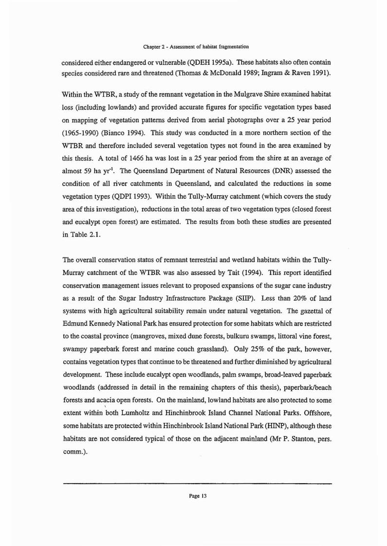
For abbreviations used in the following text see Table 2.3. Over the entire study area the

three disturbed "vegetation types" all exhibited a marked increase in total area over the 50

year period (Figure 2.4a). The single largest increase was recorded for plantation pine (6058

ha). Other large increases included almost 800% for cleared areas (CA) and over 300 ha of

sugar cane (SC). The largest reductions of remnant vegetation types were recorded for tall

eucalypt open woodlands (EOW) (78%) and low open woodlands (LOW) (56%). Melaleuca

woodlands (MW) and Melaleuca open woodlands (MOW) were reduced by 30% and 53%

Page 27

Figure 2.4


Total area (ha) of each vegetation type in 1942 and 1992.

(a) Entire area

(b) Area 1

(c) Area 2

Legend (from Table 2.3):

CA Cleared areas

MOW Melaleuca mid-high open woodlands

CFM Tall closed forests (mangroves)

EW Tall eucalypt woodlands

MW Mid-high M elaleuca woodlands

EOW Tall eucalypt open woodlands

LOW Low open woodlands

CFNM Tall closed forests (non-mangroves)

SC Sugarcane

PP Plantation pine

S Saltmarsh

Page 28

(a) 10000 J6000

4000

2000

o

n[r=:J Entire area-1942~ Entire area-1992

500

1000

(b) 48004400 ~_- -CO

..c-~ 1500coco(5I-

o

c::::J Area 1-1942 I I liii Area 1-1992 y

o~ O~ ~~ <t ~~ O~ O~ ~~ <:;;0 ~~~ (j 0 V cJ

Vegetation type

(c) 5000~ Area 2-1942

4000 Area 2-1992

3000

2000

1000

0


respectively. Relatively small decreases were recorded for mangroves (CFM) and saltmarshes (S)

(14% and 7.5 % respectively). Interestingly, both eucalypt woodlands (EW) and non-mangrove closed

forests (CFNM) exhibited an overall increase over the 50 year period.

Table 2.4 Results of variables describing remnant vegetation for the entire study area. Where

appropriate, standard errors are given in parentheses. Significant t-test results

(p~0.05) are highlighted in bold.

Variable 1942 1992 T-test p

value

Total area (ha) 23,916 17,024

Total no. of patches 515 373

Mean patch area (ha) 58.30 (8.4) 45.65 (5.33)

Mean perimeter length (km) 4.64 (0.47) 4.72 (0.43)

Mean shape index 1.88 (0.04) 2.01 (0.06)

Mean fragmentation index 2.53 (0.08) 2.39 (0.02)

Mean dispersion index 1.19 (0.36) 1.22 (0.52)

nJa

nJa

0.25

0.91

0.05

0.38

0.37

In specific areas the trends were either similar, amplified or diminished when compared with

the entire study area (Figures 2.4b and 2.4c). For example, MW were reduced by

approximately the same relative amount in each of the three areas, whereas MOW were

completely lost from Area 1, and less EOW were lost from Areas 1 and 2 compared with the

entire study area.

2.3.3 Total number of patches of vegetation types

The total number of all vegetation patches (including disturbed types) decreased from 566

to 536 over the 50 year time period. In the majority of cases, the total number of patches

of each vegetation type for each area reflected the changes in total area (Figures 2.5a-c).

Some exceptions to this are noteworthy, including an increase in the number of patches for

CFM and EOW, despite an overall reduction in the total area present. Over the entire study

Page 30

Figure 2.5


Total number of patches of each vegetation type in 1942 and 1992.

(a) Entire area

(b) Area 1

(c) Area 2


CA Cleared areas




MW Mid-high Melaleuca woodlands




SC Sugar cane

PP Plantation pine

S Saltmarsh

Page 31

(a) 120

100

80

60

40

20

o

-- .. Entire area-1942- Entire area-1992

- ~r--

-r--

r--- r--

--

-'-- '--- '-- '-I- _I- -'- '-- '-- llJ- • 1---I

(b)enQ;I.cu.....coc-

O+-oocm.....oI-

706SJ.50

40

30

20

10

o

-

'--

CI Area 2-1942.. Area 2-1992

-

--'--- ~~ _~ ~~ lIl-......n-l--,--r,__

CJ~ O~ ~~ <t ~~ O~ O~ ~~ c:P <l.<l.~ (j ~ '\; c:J-

Vegetation type

90 -r----------;:::::==========;:----..,80 70 60 -50 -40 -30 -

20 10 -0--==

(c)


area, MOW lost the highest relative proportion of patches (61 %), with MW rating second

(39%). The other most affected vegetation types were S (25%) and EW (22%). As for total

area, these figures varied between the areas examined, the most notable of which is the

complete loss of MOW from Area 1, a highly disturbed landscape.

2.3.4 Patch size class distributions of selected vegetation types

The majority of MOW patches fell within either the 0-5 ha or >30 ha size class (Figure 2.6a).

Losses in these categories were 74% and 48% respectively. As indicated above (see Section

2.3.2), MOW were completely cleared in Area 1, so all size classes in this region were lost

(Figure 2.6b). Other classes with lower frequencies lost even higher percentages across the

entire area, e.g. 83% of the 16-20 ha size class, with this class totally removed from Area

2 (Figure 2.6c).

Trends in the patch size class distributions of three other vegetation types (EW, MW and

EOW) are presented in Figures 2.7a-c. Tall eucalypt woodlands (EW) were reduced in a

similar pattern to MOW over the entire area, with the major losses occurring in both the

smallest and largest size classes. Unlike the MOW, the third size class recorded an increase

in frequency. Highest losses for MW occurred in the 41-60 ha category, with large

proportional increases and decreases in the 0~20 and 21-40 ha size classes respectively. Tall

eucalypt open woodlands (EOW) also exhibited a unique pattern of change, with the smallest

category (0-25 ha) recording a 142% increase. The largest losses were rec~rded in the 51-75

ha (57%) and >150 ha categories (70%). As for EW, a slight increase was also recorded in

the second largest patch size class.

Results of the chi-squared analyses of the size class frequency distribution and number of

patches data are presented in Table 2.5. All observed (1992) distributions were significantly

different from the expected (1942) distribution. Chi-squared values were particularly high

for size class distributions over the entire area for MOW, EW and MW. No result is

provided for MOW in Area 1 as all expected frequencies were less than 5, and the vegetation

type was absent in 1992. For the number of patches, chi-squared values were exceptionally

high for Area 1 and the entire study area.

Page 33

Figure 2.6


Patch size class distributions for mid-high Melaleuca open woodlands

(MOW) in 1942 and 1992.

(a) Entire area

(b) Area 1

(c) Area 2


CA Cleared areas

MOW M elaleuca mid-high open woodlands



MW Mid-high M elaleuca woodlands




SC Sugar cane

PP Plantation pine

S Saltmarsh

Page 34

c:J Entire area-1942.. Entire area-1992

(a) 50 -,----------~==================il

45

40

35

25201510

5o ....L.-L._

0-5 6-10 11-15 16-20 21-25 26-30 >30

(b) 4

>. 3(JcQ)

2~

0-~

LL1

0

~ Area 1-1942Area 1-1992- r-- -

- -

- r-- - ,--

I

0-5 6-10 11-15 16-20 21-25 26-30 >30

(c) 20c=J Area 2-1942

15 .. Area 2-1992

10

5

0

0-5 6-10 11-15 16-20 21-25 26-30 >30


Figure 2.7

Chapler 2 - Assessment of habitat fragmentation

Patch size class distributions for three vegetation types within the entire

study area in 1942 and 1992.

(a) Tall eucalypt woodland (EW)

(b) Mid.high Meialeuca woodlands (MW)

(c) Tall eucalypt open woodlands (EOW)

Page 36

(a) 70 ...,-----------------;::===========::;-r

65

40302010o .......L...L..---i

CJ 1942._ 1992

0-20 21-40 41-60 61-80 81-100 101-120 >120

(b) 45

>-()cCD 40~

0- 20(J)"- isu..

1050

0-20

I I 1942_ 1992

21-40 41-60 61-80 81-100 101-120 >120

I I 1942_1992

(c) 30 -r---=~----------;:::::==========:::;I

25

20

15

10

5

o ----'---'--0-25 26-50 51~75 76-100 101-125126-150 >150


Table 2.5


Results of chi-squared (Xz) analyses for different vegetation types in the study areas.

Data also includes analysis for total number of patches in the three areas examined.

All significant differences (p:50.05) are highlighted in bold. The critical 'J} values

for these tests are as follows: df=5, 11.07; df=6, 12.59; and df=8, 16.91.

Vegetation type/Area X2 df P value

MOW - Area 1

MOW - Area 2 12.93 6 0.025<p<0.05

MOW - Entire area 45.19 6 <0.001

EW - Entire area 21.39 6 0.001<p<0.005

MW - Entire area 33.79 6 <0.001

EOW - Entire area 15.91 6 0.01<p<0.025

Total number of

patches

Area 1 15.38 8 <0.001

Area 2 32.75 5 <0.001

Entire area 155.76 8 <0.001

2.3.5 Vegetation types and patch areas

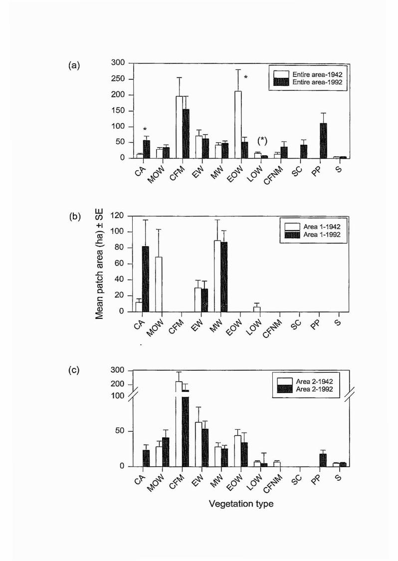
The mean patch areas of each vegetation type in 1942 and 1992, within the three different

areas, are presented in Figures 2.8a-c. Of all the vegetation types in the entire study area,

CFM and EOW (although only in 1942) had relatively high patch areas (Figure 2.8a). In

Area 1, the patch area of cleared areas (CA) had increased to greater than that of the MOW

that were present in the area in 1942 (Figure 2.8b). Melaleuca woodlands (MW) retained

relatively high patch areas here. In Area 2, mangroves (CFM) again had the highest patch

area, similar to those of the entire area recorded for PP, MOW, EW and MW (Figure 2.8c).

Page 38

Figure 2.8


Mean patch area (ha) for each vegetation type in 1942 and 1992.

Significant differences (p~O.05) are indicated with an asterisk * and linear

significant" results (O.05<p<O.1O) are indicated by an asterisk in parentheses

(*).

(a) Entire area

(b) Areal

(c) Area 2


CA Cleared areas








SC Sugar cane

PP Plantation pine

S Saltmarsh

Page 39

(a) 300

250 * ~ Entire area-1942Entire area-1992

200

150

100 *50

0

(b)ill 120C/)

+1..- 100

CO.c...- 80

CO~ 60CO.cu 40+-'

COc.. 20cCOQ.) 0~

.. Area 1-1942- Area 1-1992

-

-

-

~f -- rsI I I I I T I

(;~ o~ ~~ ~ ~~ o~ o~ ~~~ (j ~ V cJ

Vegetation type

(c)3001200100

50

o

Ic=J Area 2-1942 1.. Area 2-1992


Results of the unbalanced 3-way ANOVA indicate that for all records, patch area was

significantly different between areas and vegetation types but not time period (Table 2.6).

Where vegetation types were present in both time periods, a majority (68%) recorded a

decrease in patch area across all areas examined (Figures 2.8a-c).

Table 2.6 Results of unbalanced 3-way ANOVA's of each landscape variable and area,

vegetation type and time period. F ratios and their significance (in parentheses)

are given. Significant results (pS;0.05) are highlighted in bold and near significant

results (0.05<p<0.10) are highlighted in italics.

Variable Area Vegetation type

df 2 10

Patch area 3.06 (0.05) 17.17 (0.00)

Perimeter length 2.49 (0.08) 21.21 (0.00)

Shape index 1.10 (0.33) 26.05 (0.00)

Fragmentation index 3.30 (0.04) 17.38 (0.00)

Dispersion index 4.31 (0.01) 6.14 (0.00)

Time

1.29 (0.26)

0.13 (0.71)

6.03 (0.01)

7.41 (0.01)

1.57 (0.21)

For individual areas and time periods (I-way ANOVA), patch area was significantly different

between vegetation types, except in Area 1 in 1992 (Table 2.7). In Area 1 in 1942, although

a significant result was obtained for all vegetation types (p=O.02), no significant difference

was recorded between any two individual types. In Area 2, a majority of groups were

significantly different to CFM for both time periods (Tables Al and A2, Appendix A). For

the entire area in 1942, Tukey's HSD test indicated many types were significantly different

to CFM and EOW (Table A3, Appendix A). In 1992, however, all types except CFNM and

sugar cane (SC) were significantly different to CFM and, in addition, S and LOW were

significantly different to PP (Table A4, Appendix A).

The only significant differences for individual vegetation types over the 50 year time period

(t-test results) were recorded within the entire study area for CA and EOW, whilst LOW

recorded a "near significant" result with p=O.06 (Table 2.8a). Area I and 2 recorded no

significant differences (Tables 2.8b and 2.8c).

Page 41

Table 2.7

Chapter 2 - Assessment of habitat fragmenlation

Results of one-way ANQVA's of each landscape variable and vegetation type. F

ratios and their significance (in parentheses) are given. For significant results

(p~0.05 and highlighted in bold), multiple comparison test data (Tukey's-HSD) are

presented in Appendix A. Near significant results (O.05<p<0.10) are highlighted in

italics.

Variable Area 1 Area 2 Entire area

1942 1992 1942 1992 1942 1992

df 4 3 7 8 8 10

Patch area 3.15 1.46 9.78 9.89 8.95 4.74

(0.02) (0.24) (0.00) (0.00) (0.00) (0.00)

Perimeter length 2.15 2.22 8.91 10.97 8.22 6.01

(0.09) (0.12) (0.00) (0.00) (0.00) (0.00)

Shape index 0.75 0.80 4.97 16.92 8.26 10.27

(0.56) (0.50) (0.00) (0.00) (0.00) (0.00)

Fragmentation 2.31 0.31 2.63 10.53 23.51 3.03

index (0.07) (0.74) (0.01) (0.00) (0.00) (0.00)

Dispersion index 1.26 2.11 2.94 4.35 4.66 2.25

(0.30) (0.14) (0.01) (0.00) (0.00) (0.01)

2.3.6 Vegetation types and patch perimeter lengths

The average perimeter lengths for each vegetation type over the 50 year time period in each

of the study areas are presented in Figures 2.9a-c. As with patch area, CFM and EOW

initially had high mean perimeter lengths for the entire area. Closed forest (mangroves)

retained this high value in 1992 whereas EOW changed significantly (Figure 2.9a, Table

2.8a). Other significant differences were recorded for both CA and LOW (Table 2.8a). No

significant differences were recorded for any individual vegetation type in either Area 1 or

Page 42

Figure 2.9


Mean perimeter length (krn) for each vegetation type in 1942 and 1992.

Significant differences (p~O.05) are indicated with an asterisk * and "near

significant" results (O.05<p<O.10) are indicated by an asterisk in parentheses

(*).

(a) Entire area

(b) Areal

(c) Area 2


CA Cleared areas








SC Sugar cane

PP Plantation pine

S Saltmarsh

Page 43

(a)15

10

5 *

*

*

Cl Entire area-1942.. Entire area-1992

o

I==:J Area 1-1942l1li Area 1-1992

w(j)

(b) +1 25 ---r---------------;::====:::::=;l.........E~ 20..c.......0> 15c~~

~E

";::Q)0..CcoQ)

~

10

5

o

20 -,----------------;::::=======::::;l(c)

15

10

5

ov~ O~ ~~ <t ~~ O~ O~ ~~~ (J ~ V c:J

Vegetation type

I==:J Area 2-1942~ Area 2-1992

Table 2.8 (b)


Results of the t-tests conducted on individual vegetation types within Area 1 at the

two times examined. Significant results (p$0.05) are highlighted in bold and near

significant results (0.05<p<0.1O) are highlighted in italics. Vegetation types not

recorded in the area for both sampling times were excluded from the analysis.

Vegetation Patch Perimeter Shape Fragmentation Dispersion

type area length index index index

CA 0.15 0.13 0.21 0.21 0.16

EW 0.94 0.74 0.87 0.87 0.16

MW 0.95 0.75 0.29 0.29 0.74

Table 2.8 (c) Results of the t-tests conducted on individual vegetation types within Area 2 at the

two times examined. Significant results (pS;0.05) are highlighted in bold and near

significant results (0.05<p<0.10) are highlighted in italics. Vegetation types CA,

CFNM, SC and PP were excluded as they were only recorded in 1992.

Vegetation Patch Perimeter Shape Fragmentation Dispersion

type area length index index index

MOW 0.36 0.15 0045 0.04 0.19

CFM 0.44 0.92 0.08 0.79· 0.16

EW 0.74 0042 0.02 0.46 0.64

MW 0.74 0.63 0.50 0.31 0040

EOW 0.57 0041 0.04 0.52 0.08

LOW 0.36 0.32 0.27 0.20 0.95

S 0.62 0.92 0.60 0.01 0.62

Perimeter lengths were significantly different between vegetation types for individual areas

and times, except in Area 1 (Table 2.7). Within Area 2, CFM and EW exhibited significant

differences from most other vegetation types, particularly S (Tables A5 and A6, Appendix

A). For the entire area, most types were significantly different from both CFM and EOW

Page 46


in 1942, with S also significantly different from EW (Table A7, Appendix A). In 1992,

however, although most types remained statistically different from CFM (but not EOW),

LOW and EW were also statistically different from PP and EW (Table A8, Appendix A).

2.3.7 Vegetation types and patch shape index

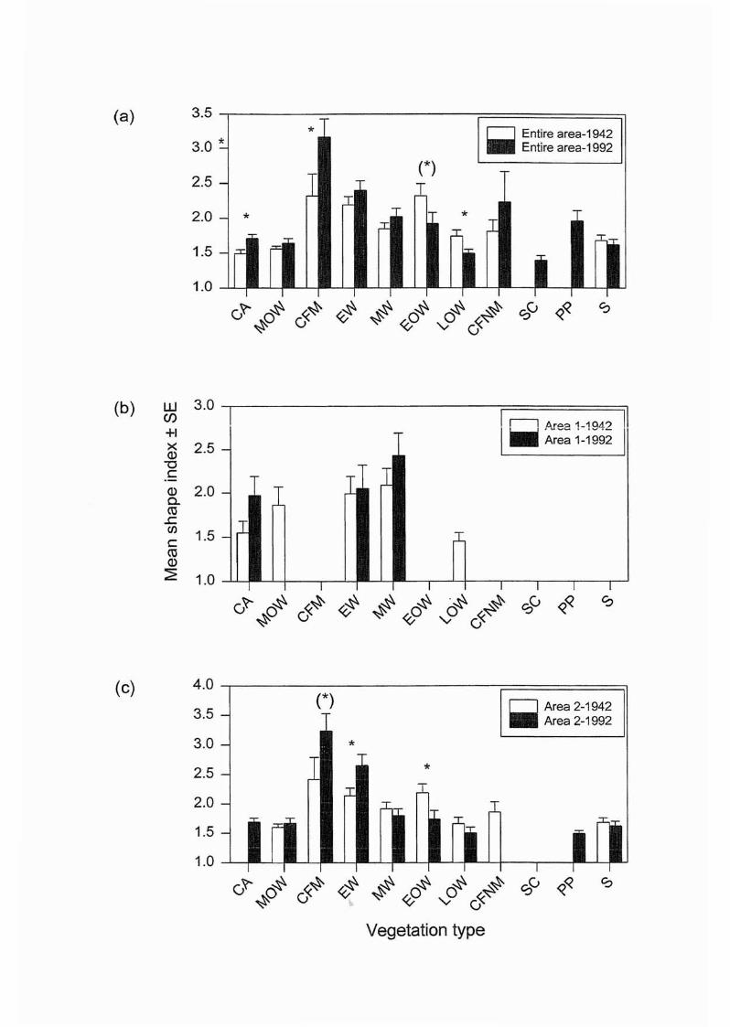
Plots of mean shape index for each vegetation type, area and time are presented in Figures

2.10a-c. Within the entire area, vegetation types with shapes closest to circularity (SI=1)

included CA, MOW, LOW and S (Figure 2.9a). Other types recorded more irregular shapes,

with CA, CFM and LOW exhibiting significant differences between times (Table 2.8a). The

latter recorded a decrease whilst CA and CFM registered an increase. Additionally, EOW

recorded a near significant decrease (p<0.10) (Table 2.8a).

Within Area 1, nearly all vegetation types had a shape index close to two at both times.

Unlike other variables examined thus far, the shape index also produced some statistically

significant results for individual vegetation types in Area 2 (Table 2.8c). These included an

increase in the irregularity of EW and a decrease in EOW. A near significant result was

recorded for the increase in the irregularity of CFM in this area (Table 2.8c). Where

particular vegetation types were present at both times, a majority (63%) across all areas

recorded an increase in the shape index (Figure 2.l0a-c).

For all data combined, the 3-way ANOVA indicated a significant difference for the shape

index between vegetation types and times, but not areas (Table 2.6). In specific areas and

times, Area 2 and the entire area recorded significant differences between vegetation types

in both times (Table 2.7). Within Area 1 for 1942, CFM, EW and EOW were significantly

different from other vegetation types, particularly MOW and S(Table A9, Appendix A). A

larger difference was recorded for CFM and EW in 1992 (Table AlO, Appendix A). These

patterns were essentially repeated over the entire study area (Tables All and AI2, Appendix

A). As with the perimeter length data, no significant results were obtained for Area 1.

Page 47

Figure 2.10


Mean shape index for each vegetation type in 1942 and 1992. Significant

differences (p~O.05) are indicated with an asterisk * and "near significant"

results (O.05<p<O.1O) are indicated by an asterisk in parentheses (*).

(a) Entire area

(b) Area 1

(c) Area 2


CA Cleared areas








SC Sugar cane

PP Plantation pine

S Saltmarsh

Page 48

(a) 3.5* • Entire area-1942

3.0 * Entire area-1992

2.5(*)

2.0 * *

1.5

1.0

(b) w 3.0(j)

+1X 2.5Q.)-ccQ.) 2.0Q..ro

..c.(/) 1.5croQ.)

::?E 1.0

• Area 1-1942

-Area 1-1992

,...

-

- .I

-'-- -'--I I I I I I

c=J Area 2-1942.. Area 2-1992

**

<t ~~ O~ O~ ~~~ V cJ

Vegetation type

4.0 I"---~-------r==========:=:;,(*)

3.5

3.0

2.5

2.0

1.5

1.0

(c)


2.3.8 Vegetation types and the fragmentation index

Results for each vegetation type, time period and area are presented in Figures 2.11a-c. This

index exhibited marked differences from the shape index. In a majority of cases (67%) a

slight decrease in this index was recorded. Five statistically significant differences were

recorded for individual vegetation types, including CA, MOW and S over the entire area

(Table 2.8a) and MOW and S in Area 2 (Table 2.8c). The largest single decrease for the

entire area was recorded for PP. For all data combined, this index is the only variable that

recorded a significant difference across areas, vegetation types and times (Table 2.6).

From the I-way ANOVA results, the dissimilarity of Area 1 (compared with both Area 2 and

the entire study area) is again apparent (Table 2.7). For Area 2 in 1942, the only pairwise

significant difference was between S and MOW (Table AB, Appendix A). In 1992,

however, many vegetation types had significant differences to PP and S, and two statistically

significant differences were recorded between LOW and both MOW and MW (Table A14,

Appendix A). In the entire area the patterns were more similar across the two time periods,

with S most significantly different (Tables A15 and A16, Appendix A). In 1942, LOW

recorded significant differences with three other vegetation types (Table A16, Appendix A).

2.3.9 Vegetation types and the dispersion index

The mean dispersion index for each vegetation type, time period and area is presented in

Figures 2.12a-c. For data combined, this index produced similar patterns to those recorded

for patch areas in that it was significantly different across both area and vegetation type, but

not time (Table 2.6).

Results from the I-way ANOVA were, however, similar to the majority of other variables

examined, i.e. vegetation types in Area 2 and the entire area recorded significant differences

for both times, whereas the vegetation types in Area 1 did not (Table 2.7). Some statistically

significant results were found in Area 2 and the entire area for pairs of vegetation types. In

Area 2 S was most significantly different from both EOW and CFM in 1942 (Table A17,

Appendix A). Fifty years later, however, saltmarsh recorded significant differences from EW

Page 50

Figure 2.11

Chapter 2 . Assessment of habitat fragmentation

Mean fragmentation index for each vegetation type in 1942 and 1992.

Significant differences (p:S;O.05) are indicated with an asterisk * and "near


(*).

(a) Entire area

(b) Areal

(c) Area 2


CA

MOW

CFM

EW

MW

EOW

Cleared areas

Melaleuca mid-high open woodlands

Tall closed forests (mangroves)

Tall eucalypt woodlands

Mid-high Melaleuca woodlands

Tall eucalypt open woodlands



SC Sugar cane

PP Plantation pine

S Saltmarsh

Page 51

*c::J Entire area-1942.. Entire area-1992

5.0 -,-;::=============~--------------,4.5

4.0

3.53.0

2.5

2.0

1.5

1.0 -'-'-~--'--

(a)

wen+1

6(b) .-N

I

0 5~-->< 4Q)"0C 3c0 2:;:;ctl....c 1Q)

E0) 0ctlL.-CctlQ)

~

• Area 1-1942- T Area 1-1992

-

-

- .:c.

- l- - --I I I I T T

*c::J Area 2-19424 - ~ Area 2-1992

(c) 5 -r;:::::============:;--------------,

3 -*

2 -

1 -

0-'- '--- '--- '-'-

Vegetation type

Figure 2.12


Mean dispersion index for each vegetation type in 1942 and 1992.

Significant differences (p~O.05) are indicated with an asterisk * and "near


(*). Values above the dotted line indicate a random distribution, while those

below the line indicate a clumped distribution.

(a) Entire area

(b) Area 1

(c) Area 2


CA Cleared areas





BOW Tall eucalypt open woodlands


CFNM Tall closed forests thon-mangroves)

SC Sugar cane

PP Plantation pine

S Saltmarsh

Page 53

4-,-;========,-----------~(a)

3

o Entire area-1942_ Entire area-1992.. ... .. > random, < clumped

2*)

**

1

o

w(b) C/)

+1 5><(])

4"CC

c 3.QC/)lo.. 2Q)0..C/)

"C 1cro 0Q)

~

c=:J Area 1-1942.. Area 1-1992........ > random, < clumped

1 - ....

o-- ~~ L.Ol~ ~- ~- ~~ -T"I--""-I

(;~ O~ ~~ ~~ ~~ O~ O~ ~~ . 0(; ««~ (j ~ v~6

Vegetation type

-'-


and CA, and CA were also different from MOW and PP (Table A18, Appendix A). For the

entire area, differences were restricted to S, and these differences were most distinct in 1942

(Tables A19 and A20, Appendix A).

The overriding trend for most vegetation types (72% of cases where a type was present in

both times) was a decrease in 1992. Most individual vegetation types retained values close

to the critical value of the dispersion index (DI=I). In the entire area PP changed from a

random to a clumped distribution, whereas EOW recorded the opposite trend (Figure 2.12a).

Both these results were statistically significant at the p~O.05 level (Table 2.8a). Cleared areas

(CA) and EOW recorded near significant results (both decreases) in the entire area and Area

2 respectively (Figures 2.12a and 2.12b, Tables 2.8a and Table 2.8c).

2.4 DISCUSSION

2.4.1 The broad picture

The annual clearing rate of remnant native vegetation recorded during this study is more than

double that found in the only other study available for lowlands in the WTBR (Bianco 1994).

The figures for the Mulgrave Shire study did, however, include upland vegetation types on

relatively steep slopes, which are characteristically cleared at much lower rates than lowland

vegetation (Catterall & Kingston 1993). Both tropical studies fall well short « 2%) of even

the long-term annual clearing rates calculated for south-eastern Queensland. This region

continues to exhibit faster population growth than any other in Australia, which has resulted

in extreme clearing rates, particularly in recent times (Catterall & Kingston 1993).

The changes in the total numbers of patches for each vegetation type across the landscape

suggest that broad-scale clearing has taken place (Figures 2.5a-c). Most types except the

disturbed classes, exhibited decreases in the numbers of patches, which indicated patches

have predominantly been lost rather than split into several new ones. In fact, it is likely that

both processes have occurred, but without a detailed assessment of the fate of individual

patches, the relative contribution of these processes cannot be determined.

For all remnant vegetation types considered collectively across the entire study area, the size

class distribution of patches has altered dramatically. Decreases in the numbers of smaller

Page 55


size class categories were the most pronounced (Figure 2.3). Most other studies (e.g.

Catterall & Kingston 1993; Mladenoff et ai. 1993; Bianco 1994) have recorded an increase

in the smaller patch size classes which may be a result of the type of clearing that has

occurred. Broad-scale clearing for urbanisation or plantation pine (mean patch areas >50 and

100 ha respectively, Figure 2.8a) has been the most common method of clearing in the area

studied during this investigation, which tends to eliminate small patches rather than create

them. The insignificant changes in most patch areas and perimeter lengths for remnant

vegetation types support the broad-scale clearing argument. The main exceptions to this are

Tall eucalypt woodlands (EW) which are discussed in more detail in Section 2.4.3, and low

open woodlands (LOW). Low open woodlands, like Melaieuca open woodlands (MOW),

were completely removed from Area 2, which has left much smaller patches (p=0.06, Table

2.8a) restricted to the southern section of the study area (Figure 2.2).

2.4.2 The landscape indices

The landscape indices for all remnant vegetation combined indicate a reduced number of

smaller patches with slightly higher perimeter lengths and significantly more irregular shapes

(Table 2.4). This is likely to render them more susceptible to edge effects which include

increases in weed invasion (Laurance 1987; Noss & Csuti 1994; Fox 1995), altered micro

climates and changes in a wide range of other ecological processes (Saunders et ai. 1991).

The perceived difference in the three separate areas chosen for closer analysis appear to have

been validated by the results of the chi-squared analysis (Table 2.5), 3-way ANOVA and 1

way ANOVA (Tables 2.6 and 2.7). Differences in landscape variables between vegetation

types (for the same time and area) are much more likely to be significant in an undisturbed

landscape (Area 2), or in a very large area exhibiting both extremes of landscape disturbance

(entire area) (Table 2.7).

The shape index produced the greatest number of significant differences between individual

vegetation types over the 50 year study period. Although a variety of shape indices have

been developed, when used in conjunction with patch size these indices are particularly

useful for studies which seek to investigate edge effects (Ripple et ai. 1991). Furthermore,

to improve the ecological interpretation of shape indices other authors have called for the

development of a shape index that takes into account both the edge to interior ratio and the

Page S6


complexity of the patch perimeter (Hulshoff 1995). Different trends (and strengths of the

trends) were recorded for different vegetation types in this study with respect to the shape

index (a significant increase for CFM and CA yet a decrease for LOW and EOW over the

same area). Increases are of most concern for remnant vegetation as they indicate a further

move from circularity, and thus an increased likelihood of management problems posed by

edge effects.

Saunders et ai. (1991) argued that a circular shape is only really important for small areas,

so it may be that for the preservation of remnants, decision making should be focused on

small areas that have exhibited an increase in the shape index. The suitability of these types

of remnants for conservation purposes would also have to be based on ecological data (i.e.

the integrity of the remnant) and weighed against resource availability as such shapes will

require more energy, time and effort to maintain their internal characteristics (Meffe &

Carroll 1994).

Of all the indices examined, only the fragmentation index (a basic area/perimeter ratio) was

significantly different over the entire area for times, area and vegetation type (Table 2.6).

Interpretation of the results for this index need to be considered carefully, as it is scale

invariant (Ripple et ai. 1991). Other authors have also indicated that simple perimeter/area

ratios should be interpreted with caution, as under some conditions different shapes can

produce similar ratios (Laurance & Yensen 1991). This index produced results very different

to those of the shape index, and was the only variable to record a significant result for

changes observed to S vegetation (Tables 2.8a and 2.8b). All other variables examined

indicate that this vegetation type has remained relatively unchanged over the 50 year time

period. In future studies this index could probably be excluded so long as some attempt to

describe patch shape is undertaken.

Changes in the dispersion index, which were significant in different directions for MOW and

EOW, could have significant ecological ramifications for these plant communities in the

landscape. Alterations to patch dispersion patterns within a landscape could feasibly affect

seed dispersal, an effect of fragmentation that is well documented, particularly for wind

dispersed species (Hopkins 1990). Flow-on effects from this change could include changes

to population heterozygosity, eventual changes in population demographics, and the rates and

types of local extinctions (Wilcox & Murphy 1985). Effects SUCh as these have, however,

Page 57


generally been subject to less research compared with the short-term effects of habitat

fragmentation documented for animal populations.

Other indices used to assess landscape pattern include patch complexity, landscape diversity,

contagion (the positive or negative association between patches) and a range of others based

on fractal geometry. Although these indices have not been investigated in this thesis, they

may provide useful insights into the data set in the future. Relatively simple indices,

however, have repeatedly been shown to adequately describe changes in landscape pattern

(e.g. Hulshoff 1995).

2.4.3 Specific vegetation types of interest

This study has provided the first detailed examination of habitat loss and fragmentation for

the tropical lowlands of north-eastern Queensland. Specific figures for each vegetation type

have enabled the most threatened ecosystems in the study area (in terms of area and shape

alterations) to be identified. Several of these are considered in more detail below.

Tall eucalypt open woodlands (EOW)

In terms of the total area of each vegetation type, EOW were the most affected by clearing

across the entire study area. The loss within this region of tropical lowlands (78%) far

exceeds the 14% estimated by QDPI (1993) for the entire catchment and even the overall

national estimate of 65% (DEST 1995b). The loss is even higher than that calculated for

south-eastern Queensland (36%), where losses of dry eucalypt communities have been second

only to M elaleuca forests (Catterall & Kingston 1993).

Approximately half of the loss (48%) recorded in this study was not actual loss per se via

clearing, but rather conversion of this open woodland to a more mesic type of vegetation.

This occurs through the invasion of vine and rainforest species, and results in a community

that is structurally similar to tall eucalypt woodlands (EW). Tall eucalypt woodlands,

although reduced in terms of total area in Area 1, exhibited an overall increase for the entire

study area, particularly in Area 2 (Figures 2.4a-c).

The process of conversion, which is believed to be the result of altered fire regimes, has long

Page 58


been of concern to national park management in the WTBR (Stanton 1989). Harrington and

Sanderson (1994) have recently quantified similar reductions in wet sclerophyll forest in the

wet tropics of Queensland following rainforest invasion. They also concluded that altered

fire regimes are the primary cause of the invasion and raise concerns regarding loss of

biodiversity from wet sclerophyll ecosystems should the process remain unchecked. No

figures for habitat conversion of lowland plant communities have been documented prior to

this study, despite the process having been observed widely in the field and identified from

vegetation pattern changes from aerial photographs (Mr P. Stanton, pers. comm.). Stanton

(1989) claims that the rapidity «30 years) of this process (which is usually irreversible in

management terms) can have significant impacts on habitat diversity in the tropical lowland

habitat mosaic. It therefore follows that overall biodiversity within the region will also be

affected.

The habitat conversion process, coupled with actual habitat loss and fragmentation (shape

index decreased significantly) has resulted in an increase in the number of smaller patches

(Figure 2.7c) and a significant decrease in patch area (Figure 2.8a). Even in a relatively

undisturbed section of the landscape, significant differences have occurred with respect to the

dispersion of this vegetation type (changing from clumped to random in Area 2, Figure

2.12c), presumably as a result of the loss of a majority of large remnant patches (Figure

2.7c). Unfortunately, no figures are available to compare the recorded extent of the

conversion process with that occurring prior 1942. In addition, it may be possible that this

conversion was exacerbated by logging activities (secondary' regrowth).

Within the WTBR, the communities being lost as a result of the conversion process are

poorly represented in the existing conservation reserve system, and have recently been

classified as vulnerable ecosystems of the region (QDEH 1995a). This assessment, although

based largely on field survey data, estimates that for the entire WTBR only 5-10% of the pre

European extent remains in an intact condition. This is despite the fact that three national

parks are located within the study area. Edmund Kennedy National Park in the north-eastern

section largely protects habitats not covered by this study (coastal beach scrubs, wetlands,

vine forests), except for MOW (Walsh 1994). Two other parks occur in the south-eastern

corner of the study area. Hinchinbrook Channel National Park largely contains mangrove

communities, and although some protection for tall open woodlands is afforded by Lumholtz

National Park, the majority of this park is not located in the coastal 10wJands.

Page 59


Melaleuca open woodlands (MOW) and woodlands (MW)

These two vegetation types have also been severely affected over the last 50 years. In Area

1 the complete loss of MOW was the only total reduction of a vegetation type recorded.

This localised reduction increases the conservation significance of remnants in other areas,

and highlights the value of considering sections of the landscape with high and low levels

of disturbance separately. This type of approach has not been adopted in previous studies,

which have traditionally focused on large areas of landscape, quite often at scales well above

the one chosen for use here. In contrast, MW were one of the least affected vegetation types

in Area 1.

In terms of patch size class distributions, MOW are again unique in that they had the highest

loss of patches in the smallest size class (0-5 ha), the complete loss of a size class in Area

2 and the second largest loss of large patches for the entire area (Figures 2.6a-c). Despite

these massive changes, the only landscape indices to alter significantly were the dispersion

index for the entire area (changing from random to clumped) and a decrease in the

fragmentation index in Area 2. This indicates that apart from distribution across the

landscape, the shape characteristics of this vegetation type have remained essentially

unchanged. No significant changes were recorded for MW for any of the indices used.

Melaleuca open woodlands have recently been classified as a vulnerable ecosystem (QDEH

1995a). Despite preservation in two mainland national parks in the study area (Lumholtz and

Edmund Kennedy National Parks), regional representation of this vegetation type within the

WTBR remains limited (Walsh 1994). These woodlands are the focus of the research

presented in Chapters 3-6 of this thesis.

2.4.4 Management implications for fragmented lands~apes

Fragmented landscapes pose perhaps the greatest challenge to conservation management in

Australia. Without active management small, irregularly shaped remnants prone to edge

effects and external influences have questionable long-term viabilities (House & Moritz

1991), and may not continue to support native plant and animal communities (Saunders et

al. 1993). In fact, the decline and localised extinction of many plant and animal species from

small, isolated remnants has been repeatedly demonstrated both in Austr~lia (e.g. Saunders

Page 60


& Hobbs 1995) and overseas (e.g. Myers 1994).

The relevance of landscape pattern infonnation derived from indices to conservation

questions has not been fully demonstrated (Noss & Csuti 1994). Indeed, it could be argued

that this type of infonnation is only relevant for the design of future nature reserves in

relatively undisturbed landscapes. The ability of indices to facilitate patch selection and edge

design in variously disturbed environments has, however, been demonstrated (Buechner 1987;

Fensham submitted). Results from this investigation also suggest that critical communities

for conservation initiatives can be identified in highly disturbed sections of the landscape.

The powerful nature of the time series approach to landscape analysis for use as a monitoring

tool has also been observed (Noss 1990).

Most conservation planning exercises have been based primarily on the present distribution

of plant communities, with little infonnation on historical patterns available. This is

particularly true in the lowland vegetation mosaic of the north-eastern tropics. Infonnation

gained from studies such as these is essential so that priorities for conservation can be

fonnulated based on a knowledge of past clearing patterns, and therefore an appreciation of

which communities are truly threatened. For example, as a result of this study, arguments

for increased representation of the three communities discussed in Section 2.4.3 within the

conservation reserve system can be fonnulated. In fact, an increasing number of studies are

now illustrating the disappointingly poor results achieved in tenns of overall biodiversity

conservation when reserve selection (as it has traditionally been) is essentially ad hoc

(Lambeck 1994). Ever increasing recognition is also being given to a combination of on

and off-park conservation measures (Taylor 1993; Wells et al. 1994; Fensham submitted),

with the emphasis on planning in an integrated fashion at the landscape scale (Saunders et

al. 1993).

Following a detailed study of remnant bushland in south-eastern Queensland, Catterall and

Kingston (1993) proposed a framework and priorities for conservation of vegetation in

fragmented landscapes. Many management issues are equally important, including altered

hydrological patterns (particularly drainage), changes in fire regimes and the invasion of

exotic species. The effects of the latter two problems are considered in more detail for MOW

in Chapters 3/5 and 6 respectively. These effects may be difficult to differentiate from those

of habitat loss and fragmentation.

Page 61


The mitigation of these external influences and the control of internal patch dynamics is

critical if the long-tenn viabilities of remnants are to be maintained (Saunders et ai. 1991).

Indeed, studying the internal dynamics of isolated remnants can help identify processes that

can act as early warning indicators for the management of larger remnants in the landscape

as they continue to fragment (Given 1994). Management also has to address the various

scales at which these effects operate, from the level of meta-populations right through to the

level of individual species. At the same time, whilst trying to appreciate that the responses

of specific taxa to the many and varied effects of fragmentation can differ considerably,

modern day conservation managers also have to contend with a wide range of constraining

realities including funding (or the lack thereof) for land acquisition, land tenure, development

pressures, clearing guidelines (currently being developed for leasehold land in Queensland,

DoL 1995) and other legislative issues.

Page 62

Skull, Stephen David (1998) The ecology of tropical ... · This file is part of the following reference: Skull, Stephen David (1998) The ecology of tropical lowland plant communities

Documents