S.J.J.M.F. Kokkelmans et al- Resonance Superfluidity: Renormalization of Resonance Scattering Theory

8/3/2019 S.J.J.M.F. Kokkelmans et al- Resonance Superfluidity: Renormalization of Resonance Scattering Theory

http://slidepdf.com/reader/full/sjjmf-kokkelmans-et-al-resonance-superfluidity-renormalization-of-resonance 1/15

a r X i v : c o n d - m a t / 0 1 1 2 2 8 3 v 1

1 5 D e c 2 0 0 1

Resonance Superfluidity: Renormalization of Resonance Scattering Theory

S.J.J.M.F. Kokkelmans1, J.N. Milstein1, M.L. Chiofalo2, R. Walser1, and M.J. Holland11JILA, University of Colorado and National Institute of Standards and Technology, Boulder, Colorado 80309-0440, U.S.A.

2INFM and Classe di Scienze, Scuola Normale Superiore, Piazza dei Cavalieri 7, I-56126, Pisa, Italy

(December 18, 2001)

We derive a theory of superfluidity for a dilute Fermi gas that is valid when scattering resonancesare present. The treatment of a resonance in many-body atomic physics requires a novel mean-

field approach starting from an unconventional microscopic Hamiltonian. The mean-field equationsincorporate the microscopic scattering physics, and the solutions to these equations reproduce theenergy-dependent scattering properties. This theory describes the high-T c behavior of the system,and predicts a value of T c which is a significant fraction of the Fermi temperature. It is shown thatthis novel mean-field approach does not break down for typical experimental circumstances, evenat detunings close to resonance. As an example of the application of our theory we investigate thefeasibility for achieving superfluidity in an ultracold gas of fermionic 6Li.

PACS: 03.75.Fi,67.60.-g,74.20.-z

I. INTRODUCTION

The remarkable accomplishment of reaching the regimeof quantum degeneracy [1] in a variety of ultracold atomicgases enabled the examination of superfluid phenomenain a diverse range of novel quantum systems. Alreadymany elementary aspects of superfluid phenomena havebeen observed in bosonic systems including vortices [2].The challenge of achieving superfluidity in a Fermi gas re-mains, however, although it appears possible that this sit-uation may change in the near future. A number of can-didate systems for realizing superfluidity in a fermionicgas appear very promising and it is currently the goalof several experimental efforts to get into the requiredregime to observe the superfluid phase transition. So farboth fermionic potassium [3] and lithium [4,5] have been

cooled to the microkelvin regime and are well below theFermi temperature by now—a precursor step for super-fluidity.

In order to make the superfluid phase transition exper-imentally accessible, it will likely be necessary to utilizethe rich internal hyperfine structure of atomic collisions.Scattering resonances, in particular, may prove to be ex-tremely important since they potentially allow a signifi-cant enhancement of the strength of the atomic interac-tions. It is anticipated that by utilizing such a scatteringresonance one may dramatically increase the critical tem-perature at which the system becomes unstable towardsthe formation of Cooper pairs, thus bringing the critical

temperature into the experimentally accessible regime.In spite of its promise, this situation poses a numberof fundamental theoretical problems which must be ad-dressed in order to provide an adequate minimal descrip-tion of the critical behavior. The scope of the complex-ities that arise in treating a scattering resonance can beseen by examining the convergence of the quantum ki-netic perturbation theory of the dilute gas. In this theorythe small parameter is known as the gaseous parameter;defined as

√na3 where n is the particle density and a

is the scattering length. Formally, when the scatteringlength is increased to the value at which na3 ≈ 1, conven-tional perturbation theory breaks down [6,7]. This situ-

ation is commonly associated with the theoretical treat-ment of strongly interacting fermionic systems wherehigh-order correlations must be treated explicitly.

In this paper, we show that an unconventional mean-field theory can still be appropriately exploited underthe condition that the characteristic range R of the po-tential is such that nR3 1 (while na3 >∼ 1). The coreissue is that around a resonance, the cross-section be-comes strongly dependent on the scattering energy. Thisoccurs when either a bound state lies just below thresh-old, or when a quasi-bound state lies just above the edgeof the collision continuum. In both cases, the scatteringlength—evaluated by considering the zero energy limit

of the scattering phase shift—does not characterize thefull scattering physics over the complete energy range of interest, even when in practice this may cover a range of only a few microkelvin.

The paper is outlined as follows. In Section II, wepresent a systematic derivation of the renormalized po-tentials for an effective many-body Hamiltonian. Thisrequires a detailed analysis of coupled-channels scatter-ing. In Section III, we derive the resonance mean-fieldtheory. In Section IV, we present the thermodynamicsolutions allowing for resonance superfluidity. We applyour theory to the specific case of 6Li and determine thecritical temperature for the superfluid phase transition.In Section V, we consider the validity of the mean fieldapproach in the case of resonance coupling, and establishthe equivalence with previous diagrammatic calculationsof the crossover regime between fermionic and bosonicsuperconductivity.

1



II. TWO-BODY RESONANCE SCATTERING

The position of the last bound state in the interatomicinteraction potentials generally has a crucial effect onthe scattering properties. In a single-channel system,the scattering process becomes resonant when a boundstate is close to threshold. In a multi-channel system theincoming channel (which is always open) may be cou-

pled during the collision to other open or closed channelscorresponding to different spin configurations. When abound state in a closed channel lies near the zero of thecollision energy continuum, a Feshbach resonance [8] mayoccur, giving rise to scattering properties which are tun-able by an external magnetic field. The tuning depen-dence arises from the magnetic moment difference ∆µmag

between the open and closed channels [9]. This gives riseto a characteristic dispersive behavior of the s-wave scat-tering length at fields close to resonance given by

a = abg

1 − ∆B

B − B0

, (1)

where abg is the background value which may itself de-pend weakly on magnetic field. The field-width of theresonance is given by ∆B, and the bound state crossesthreshold at a field-value B0. The field-detuning canbe converted into an energy-detuning ν by the relationν = (B − B0)∆µmag. An example of such a resonanceis given in Fig. 1, where a coupled channels calculationis shown of the scattering length of 6Li for collisions be-tween atoms in the (f, mf ) = (1/2,−1/2) and (1/2, 1/2)state [10]. The background scattering length changesslowly as a function of magnetic field due to a field-dependent mixing of a second resonance which comesfrom the triplet potential. This full coupled channels

calculation includes the state-of-the-art interatomic po-tentials [11] and the complete internal hyperfine struc-ture [13].

0 200 400 600 800 1000 1200−5000

−2500

0

2500

5000

B (G)

a

( U n i t s o f a 0

)

FIG. 1. Scattering length as a function of magnetic field,for the (f, mf ) = (1/2,−1/2) and (1/2, 1/2) mixed spin chan-nel of 6Li.

The scattering length is often used in many-bodytheory to describe interactions in the s-wave regime.That the scattering length completely encapsulates thecollision physics over relevant energy scales is implic-itly assumed in the derivation of the conventionalBardeen-Cooper-Schrieffer (BCS) theory for degenerategases [14,15], as well as the Gross-Pitaevskii descriptionof Bose-Einstein condensates. However, the scattering

length is only a useful concept in the energy regime wherethe s-wave scattering phase shift δ0 depends linearly onthe wavenumber k, i.e. δ0 = −ka. For a Feshbach reso-nance system at a finite temperature there will always bea magnetic field value where this approximation breaksdown and the scattering properties become strongly en-ergy dependent. In close proximity to a resonance, thescattering process then has to be treated by means of theenergy dependent T -matrix.

Only the exact interatomic interaction will reproducethe full T -matrix over all energy scales. However, sinceonly collision energies in the ultracold regime (of ordermicrokelvin) are relevant, a much simpler description ispossible. If the scattering length does not completelycharacterize the low energy scattering behavior in thepresence of a resonance, what is the minimal set of pa-rameters which do?

As illustrated in Fig. 2, we proceed to systematicallyresolve this question by the following steps. We startfrom a numerical solution of the complete coupled chan-nels scattering problem for a given real physical system.In Section II A we demonstrate that the results of thesefull numerical calculations can be adequately replicatedby giving an analytic description of resonance scatteringprovided by Feshbach’s resonance theory. The point of this connection is to demonstrate that only a few param-eters are necessary to account for all the collision proper-

ties. This implies that the scattering model is not unique.There are many microscopic models which could be de-scribed by the same Feshbach theory. In Section II Bwe show this explicitly by presenting a simple doublewell model for which analytic solutions are accessible.Thereby we derive a limiting model in which the range of the square well potentials and coupling matrix elementsare taken to zero. This leads in Section II C to a scat-tering model of contact potentials. We show that such ascattering solution is able to reproduce well the resultsof the intricate full numerical model we began with. Theutility of this result is that, as will be apparent later, itgreatly simplifies the many-body theoretic description.

2



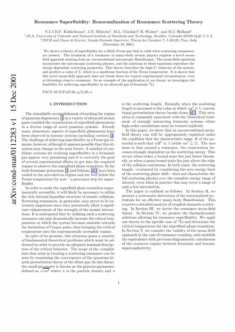
Full CC scattering

Feshbach scattering

Square-well scattering

Contact scattering

FIG. 2. Sequence of theoretical steps involved in formu-

lating a renormalized scattering model of resonance physicsfor low energy scattering. The starting point is a full coupledchannels (CC) calculation, which leads via an equivalent Fes-hbach theory, and an analytic coupled square well theory, toa contact potential scattering theory which gives the renor-malized equations for the resonance system.

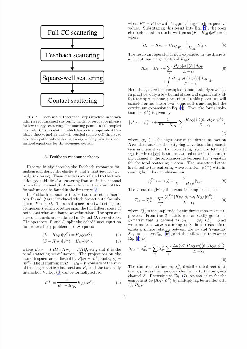
A. Feshbach resonance theory

Here we briefly describe the Feshbach resonance for-malism and derive the elastic S - and T -matrices for two-body scattering. These matrices are related to the tran-sition probabilities for scattering from an initial channelα to a final channel β . A more detailed treatment of thisformalism can be found in the literature [ 8].

In Feshbach resonance theory two projection opera-tors P and Q are introduced which project onto the sub-spaces P and Q. These subspaces are two orthogonalcomponents which together span the full Hilbert space of both scattering and bound wavefunctions. The open andclosed channels are contained in P and Q, respectively.The operators P and Q split the Schrodinger equationfor the two-body problem into two parts:

(E −H P P )|ψP = H P Q|ψQ, (2)

(E

−H QQ)

|ψQ

= H QP

|ψP

, (3)

where H P P = P HP , H P Q = P H Q, etc., and ψ is thetotal scattering wavefunction. The projections on thetwo sub-spaces are indicated by P |ψ = |ψP and Q|ψ =|ψQ. The Hamiltonian H = H 0 + V consists of the sumof the single-particle interactions H 0 and the two-bodyinteraction V . Eq. (3) can be formally solved

|ψQ =1

E + −H QQ

H QP |ψP , (4)

where E + = E +iδ with δ approaching zero from positivevalues. Substituting this result into Eq. (2), the openchannels equation can be written as (E −H eff )|ψP = 0,where

H eff = H P P + H P Q1

E + −H QQ

H QP . (5)

The resolvant operator is now expanded in the discrete

and continuum eigenstates of H QQ:

H eff = H P P +

i

H P Q|φiφi|H QP

E − i

(6)

+

H P Q|φ()φ()|H QP

E + − d.

Here the i’s are the uncoupled bound-state eigenvalues.In practice, only a few bound states will significantly af-fect the open-channel properties. In this paper, we willconsider either one or two bound states and neglect thecontinuum expansion in Eq. (6). Then the formal solu-tion for |ψP is given by

|ψP = |ψP +α +1

E + −H P P

i

H P Q

|φi

φi

|H QP

|ψP

E − i,

(7)

where |ψP +α is the eigenstate of the direct interaction

H P P that satisfies the outgoing wave boundary condi-tion in channel α. By multiplying from the left withχβ|V , where |χβ is an unscattered state in the outgo-ing channel β , the left-hand-side becomes the T -matrixfor the total scattering process. The unscattered stateis related to the scattering wave-function |ψP −

β with in-coming boundary conditions via

|ψP −

β =|χβ

+

V

E − −H P P |χβ

. (8)

The T -matrix giving the transition amplitude is then

T βα = T P βα +

i

ψP −β |H P Q|φiφi|H QP |ψP

E − i

, (9)

where T P βα is the amplitude for the direct (non-resonant)

process. From the T -matrix we can easily go to theS -matrix that is defined as S βα = ψ−

β |ψ+α . Since

we consider s-wave scattering only, in our case thereexists a simple relation between the S - and T -matrix:S βα = 1 − 2πiT βα [16], and this allows us to rewriteEq. (9) as

S βα = S P βα −

γ

S P βγ

i

2πiψ+γ |H P Q|φiφi|H QP |ψP E − i

.

(10)

The non-resonant factors S P βγ describe the direct scat-

tering process from an open channel γ to the outgoingchannel β . Returning to Eq. (7), we can solve for thecomponent φi|H QP |ψP by multiplying both sides withφi|H QP .

3



1. Single resonance

For the case of only one resonant bound state and onlyone open channel, the solution of Eq. (7) gives rise to thefollowing elastic S -matrix element (we will omit now theincoming channel label α):

S = S P

1 −2πi

|ψP +

|H P Q

|φ1

|2

E − 1 − φ1|H QP 1

E+−H PP H P Q|φ1 .

(11)

The non-resonant S -matrix is related to the backgroundscattering length via S P = exp[−2ikabg]. The term inthe numerator gives rise to the energy-width of the res-onance, Γ = 2π|ψP +|H P Q|φ1|2, which is proportionalto the incoming wavenumber k and coupling constant g1[17]. The bracket in the denominator gives rise to a shiftof the bound-state energy, and to an additional widthterm iΓ/2. When we denote the energy-shift betweenthe collision continuum and the bound state by ν 1, and

represent the kinetic energy simply by h

2

k2

/m, the S -matrix element can be rewritten as

S (k) = e−2ikabg

1 − 2ik|g1|2

−4πh2

m(ν 1 − h2k2

m) + ik|g1|2

. (12)

The resulting total scattering length has exactly the dis-persive lineshape for the resonant scattering length whichwe presented originally as Eq. (1).

2. Double resonance

Often more than one resonance may need to be con-sidered. For example, the scattering properties for the(1/2,−1/2) + (1/2, 1/2) channel of 6Li are dominatedby a combination of two resonances: a triplet poten-tial resonance and a Feshbach resonance. This can beclearly seen from Fig. 1, where the residual scatteringlength, which would arise in the absence of the Fesh-bach resonance coupling, would be very large and nega-tive and vary with magnetic field. This can be comparedwith the value of the non-resonant background scatter-ing length for the triplet potential for Li which is only31 a0, which is an accurate measure of the characteristicrange of this potential. An adequate scattering model forthis system therefore requires inclusion of both bound-

state resonances. Since for 6Li the coupling betweenthese two bound states is small, it will be neglected inthe double resonance model presented here. The double-resonance S -matrix, with again only one open channel,follows then from Eq. (10) and includes a summation overtwo bound states. After solving for the two componentsφi|H QP |ψP of wave function |ψP , the S -matrix can bewritten as

S (k) = e−2ikabg

1 − 2ik(|g1|2∆2 + |g2|2∆1)

ik(|g1|2∆2 + |g2|2∆1) −∆1∆2

.

(13)

with ∆1 = (ν 1 − h2k2/m)4πh2/m, where ν 1 and g1 arethe detuning and coupling strengths for state 1. Equiva-lent definitions are used for state 2. Later we will showthat this simple analytic Feshbach scattering model mim-

ics the coupled channels calculation of 6Li. The parame-ters of this model, which are related to the positions andwidths of the last bound states, can be directly foundfrom a plot of the scattering length versus magnetic fieldas given, for example, by Fig. 1. The scattering lengthbehavior should be reproduced by the analytic expressionfor the scattering length following from Eq. (13):

a = abg − m

4πh2

|g1|2ν 1

+|g2|2

ν 2

. (14)

The advantage of a double-pole over a single-pole S -matrix parametrisation is that we can account for the

interplay between a potential resonance and a Feshbachresonance, which in principle can radically change thescattering properties. This interplay is not only im-portant for the description of 6Li interactions, but alsofor other atomic systems which have an almost resonanttriplet potential, such as bosonic 133Cs [18,19] and 85Rb[20].

In the many-body part of this paper, Section III, thescattering properties are represented by a T -matrix in-stead of an S -matrix. We have shown in the above thatin our case there exists a simple relation between the two,however, the definition for T in the many-body theorywill be slightly different in order to give it the conven-tional dimensions of energy per unit density:

T (k) =2πh2i

mk[S (k) − 1] . (15)

4



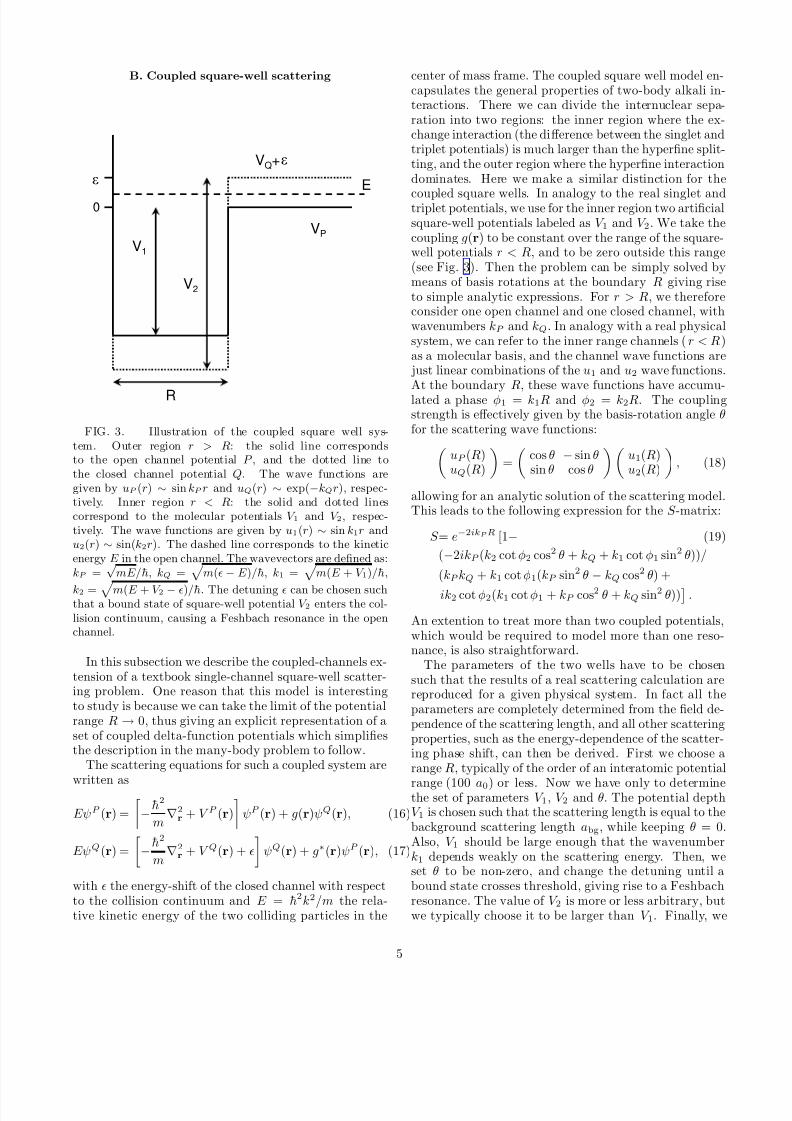
B. Coupled square-well scattering

V1

V2

VQ+

VP

E

0

R

FIG. 3. Illustration of the coupled square well sys-tem. Outer region r > R: the solid line correspondsto the open channel potential P , and the dotted line tothe closed channel potential Q. The wave functions aregiven by uP (r) ∼ sin kP r and uQ(r) ∼ exp(−kQr), respec-tively. Inner region r < R: the solid and dotted linescorrespond to the molecular potentials V 1 and V 2, respec-tively. The wave functions are given by u1(r) ∼ sin k1r andu2(r) ∼ sin(k2r). The dashed line corresponds to the kineticenergy E in the open channel. The wavevectors are defined as:kP =

√mE/h, kQ = m(− E )/h, k1 = m(E + V 1)/h,

k2 =

m(E + V 2 − )/h. The detuning can be chosen suchthat a bound state of square-well potential V 2 enters the col-lision continuum, causing a Feshbach resonance in the openchannel.

In this subsection we describe the coupled-channels ex-tension of a textbook single-channel square-well scatter-ing problem. One reason that this model is interestingto study is because we can take the limit of the potentialrange R → 0, thus giving an explicit representation of aset of coupled delta-function potentials which simplifiesthe description in the many-body problem to follow.

The scattering equations for such a coupled system are

written as

EψP (r) =

− h2

m2r + V P (r)

ψP (r) + g(r)ψQ(r), (16)

EψQ(r) =

− h2

m2r + V Q(r) +

ψQ(r) + g∗(r)ψP (r), (17)

with the energy-shift of the closed channel with respectto the collision continuum and E = h2k2/m the rela-tive kinetic energy of the two colliding particles in the

center of mass frame. The coupled square well model en-capsulates the general properties of two-body alkali in-teractions. There we can divide the internuclear sepa-ration into two regions: the inner region where the ex-change interaction (the difference between the singlet andtriplet potentials) is much larger than the hyperfine split-ting, and the outer region where the hyperfine interactiondominates. Here we make a similar distinction for the

coupled square wells. In analogy to the real singlet andtriplet potentials, we use for the inner region two artificialsquare-well potentials labeled as V 1 and V 2. We take thecoupling g(r) to be constant over the range of the square-well potentials r < R, and to be zero outside this range(see Fig. 3). Then the problem can be simply solved bymeans of basis rotations at the boundary R giving riseto simple analytic expressions. For r > R, we thereforeconsider one open channel and one closed channel, withwavenumbers kP and kQ. In analogy with a real physicalsystem, we can refer to the inner range channels (r < R)as a molecular basis, and the channel wave functions are

just linear combinations of the u1 and u2 wave functions.At the boundary R, these wave functions have accumu-lated a phase φ1 = k1R and φ2 = k2R. The couplingstrength is effectively given by the basis-rotation angle θfor the scattering wave functions:

uP (R)uQ(R)

=

cos θ − sin θsin θ cos θ

u1(R)u2(R)

, (18)

allowing for an analytic solution of the scattering model.This leads to the following expression for the S -matrix:

S = e−2ikP R [1− (19)

(−2ikP (k2 cot φ2 cos2 θ + kQ + k1 cot φ1 sin2 θ))/

(kP kQ + k1 cot φ1(kP sin2 θ

−kQ cos2 θ) +

ik2 cot φ2(k1 cot φ1 + kP cos2 θ + kQ sin2 θ))

.

An extention to treat more than two coupled potentials,which would be required to model more than one reso-nance, is also straightforward.

The parameters of the two wells have to be chosensuch that the results of a real scattering calculation arereproduced for a given physical system. In fact all theparameters are completely determined from the field de-pendence of the scattering length, and all other scatteringproperties, such as the energy-dependence of the scatter-ing phase shift, can then be derived. First we choose arange R, typically of the order of an interatomic potential

range (100 a0) or less. Now we have only to determinethe set of parameters V 1, V 2 and θ. The potential depthV 1 is chosen such that the scattering length is equal to thebackground scattering length abg, while keeping θ = 0.Also, V 1 should be large enough that the wavenumberk1 depends weakly on the scattering energy. Then, weset θ to be non-zero, and change the detuning until abound state crosses threshold, giving rise to a Feshbachresonance. The value of V 2 is more or less arbitrary, butwe typically choose it to be larger than V 1. Finally, we

5



change the value of θ to give the Feshbach resonance thedesired width.

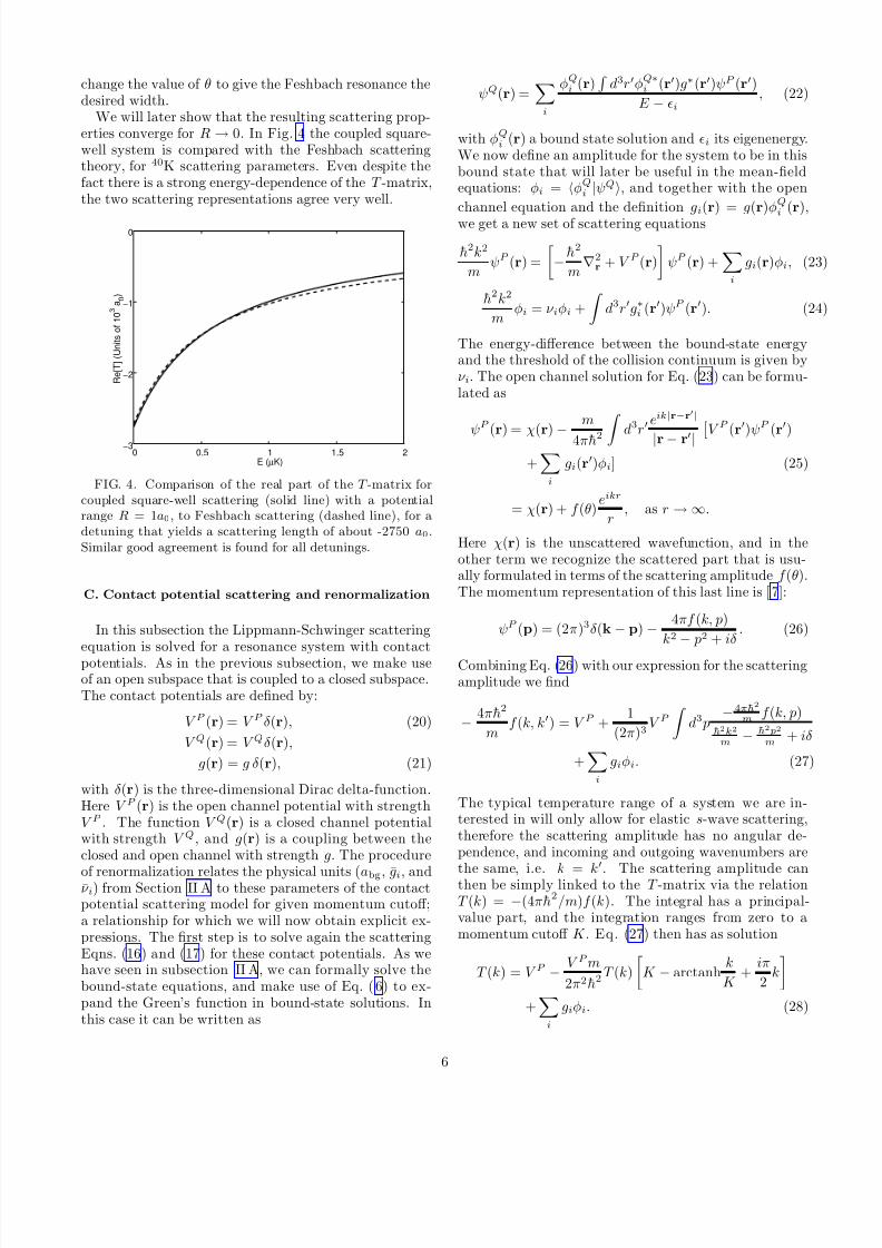
We will later show that the resulting scattering prop-erties converge for R → 0. In Fig. 4 the coupled square-well system is compared with the Feshbach scatteringtheory, for 40K scattering parameters. Even despite thefact there is a strong energy-dependence of the T -matrix,the two scattering representations agree very well.

0 0.5 1 1.5 2−3

−2

−1

0

E (µK)

R e [ T ] ( U n i t s o f 1 0

3 a 0

)

FIG. 4. Comparison of the real part of the T -matrix forcoupled square-well scattering (solid line) with a potentialrange R = 1a0, to Feshbach scattering (dashed line), for adetuning that yields a scattering length of about -2750 a0.Similar good agreement is found for all detunings.

C. Contact potential scattering and renormalization

In this subsection the Lippmann-Schwinger scatteringequation is solved for a resonance system with contactpotentials. As in the previous subsection, we make useof an open subspace that is coupled to a closed subspace.The contact potentials are defined by:

V P (r) = V P δ(r), (20)

V Q(r) = V Qδ(r),

g(r) = g δ(r), (21)

with δ(r) is the three-dimensional Dirac delta-function.Here V P (r) is the open channel potential with strengthV P . The function V Q(r) is a closed channel potentialwith strength V Q, and g(r) is a coupling between theclosed and open channel with strength g. The procedure

of renormalization relates the physical units (abg, gi, andν i) from Section II A to these parameters of the contactpotential scattering model for given momentum cutoff;a relationship for which we will now obtain explicit ex-pressions. The first step is to solve again the scatteringEqns. (16) and (17) for these contact potentials. As wehave seen in subsection II A, we can formally solve thebound-state equations, and make use of Eq. (6) to ex-pand the Green’s function in bound-state solutions. Inthis case it can be written as

ψQ(r) =

i

φQi (r)

d3rφQ∗

i (r)g∗(r)ψP (r)

E − i

, (22)

with φQi (r) a bound state solution and i its eigenenergy.

We now define an amplitude for the system to be in thisbound state that will later be useful in the mean-fieldequations: φi = φQ

i |ψQ, and together with the open

channel equation and the definition gi(r) = g(r)φQi (r),

we get a new set of scattering equations

h2k2

mψP (r) =

− h2

m2r + V P (r)

ψP (r) +

i

gi(r)φi, (23)

h2k2

mφi = ν iφi +

d3rg∗i (r)ψP (r). (24)

The energy-difference between the bound-state energyand the threshold of the collision continuum is given byν i. The open channel solution for Eq. (23) can be formu-lated as

ψP (r) = χ(r)−

m

4πh2 d3r

eik|r−r|

|r− r| V P (r)ψP (r)

+

i

gi(r)φi] (25)

= χ(r) + f (θ)eikr

r, as r →∞.

Here χ(r) is the unscattered wavefunction, and in theother term we recognize the scattered part that is usu-ally formulated in terms of the scattering amplitude f (θ).The momentum representation of this last line is [7]:

ψP (p) = (2π)3δ(k − p) − 4πf (k, p)

k2

− p2 + iδ

. (26)

Combining Eq. (26) with our expression for the scatteringamplitude we find

− 4πh2

mf (k, k) = V P +

1

(2π)3V P

d3 p

−4πh2

mf (k, p)

h2k2

m− h2 p2

m+ iδ

+

i

giφi. (27)

The typical temperature range of a system we are in-terested in will only allow for elastic s-wave scattering,therefore the scattering amplitude has no angular de-pendence, and incoming and outgoing wavenumbers are

the same, i.e. k = k

. The scattering amplitude canthen be simply linked to the T -matrix via the relationT (k) = −(4πh2/m)f (k). The integral has a principal-value part, and the integration ranges from zero to amomentum cutoff K . Eq. (27) then has as solution

T (k) = V P − V P m

2π2h2T (k)

K − arctanh

k

K +

iπ

2k

+

i

giφi. (28)

6



This is a variant of the Lippmann-Schwinger equation.The closed channel scattering solutions are now used toeliminate the amplitude functions φi. In Fourier space,Eq. (24) has the form

h2k2

mφi = ν iφi + g∗i

1

(2π)3

ψP (p)d3 p. (29)

After substitution of Eq. (26) the expression for φi islinked to the T -matrix:

φi =g∗i

1 − m2π2h2

T (k)

K − arctanh kK

+ iπ2

k

h2k2

m− ν i

. (30)

Eliminating φi from Eq. (28) gives a complete expressionfor the Lippmann-Schwinger equation

T (k) = V P − V P m

2π2h2 T (k)

K − arctanh

k

K +

iπ

2k

+

i

|gi|2

1 − 12π2

mh2

T (k)

K − arctanh kK

+ iπ2

k

h2k2

m

−ν i

. (31)

Similar to the Feshbach and coupled square-well prob-lems, the k → 0 behavior of T (k) should reproduce thescattering length, and, the result should not depend onthe arbitrary momentum cutoff K . For an analytic ex-pression of the scattering length, we conveniently use theFeshbach representation. A comparison between the lat-ter and the expression for the scattering length a thatresults from solving Eq. (31), tells us how to relate thecoupling constants for contact-scattering to the Feshbachcoupling constants. By making use of the definitionsΓ = (1−αU )−1, α = mK/(2π2h2), and U = 4πh2abg/m,we find the very concise relations

V P = ΓU, (32)

which is valid also in the case where no resonance ispresent, and in addition

g1 = Γg1, (33)

ν 1 = ν 1 + αg1g1. (34)

for the open channel potential and the first resonance.For the second resonance, if present, we find

g2 =g2

αg21/ν 1 + Γ−1, (35)

ν 2 = ν 2 + αg2g2. (36)

Obviously, our approach an be systematically extendedfurther, order by order, to give an arbitrarily accuraterepresentation of the microscopic scattering physics.

These expressions we refer to as the renormalizingequations of the resonance theory since they remove theultra-violet divergence which would otherwise appear inthe field-equations. Any many-body theory based on con-tact scattering around a Feshbach resonance will need to

apply these expressions in order to renormalize the the-ory. These equations (32)-(36) therefore represent one of the major results of this paper.

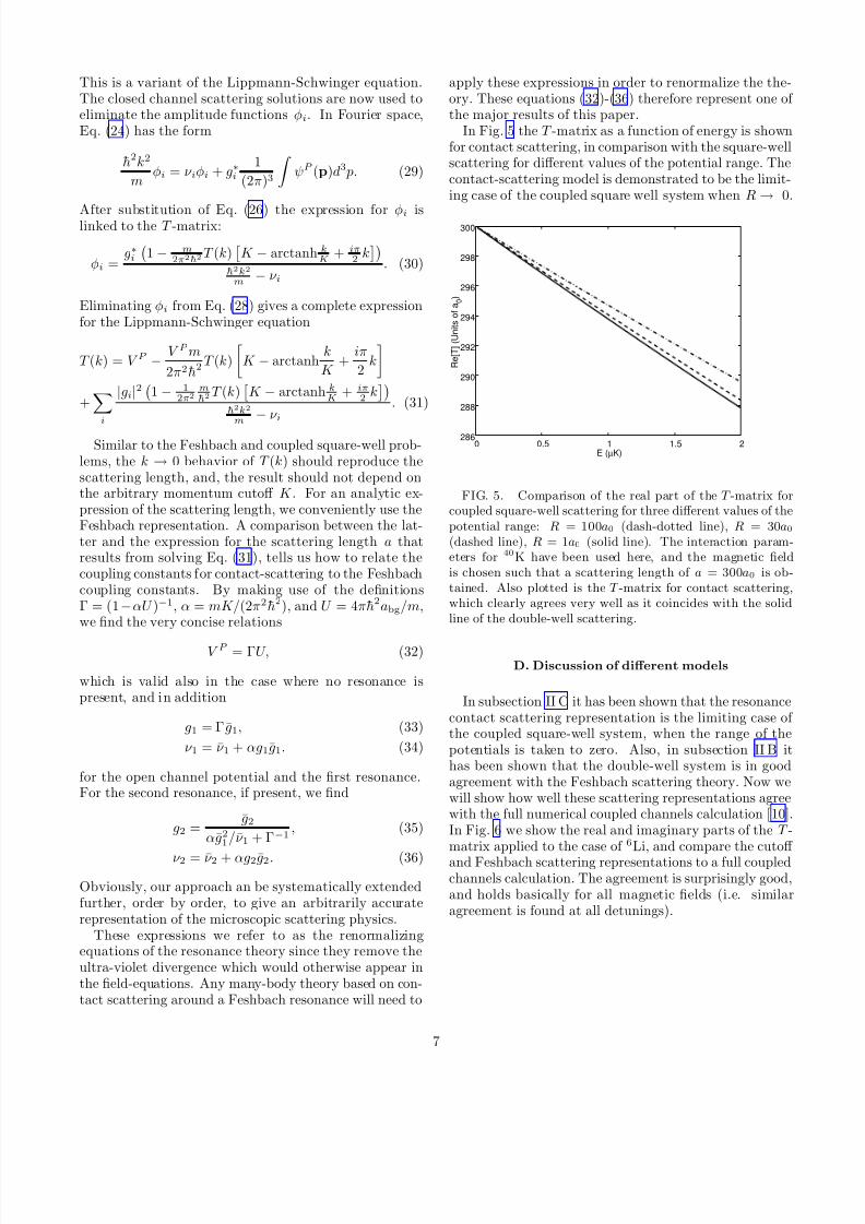
In Fig. 5 the T -matrix as a function of energy is shownfor contact scattering, in comparison with the square-wellscattering for different values of the potential range. Thecontact-scattering model is demonstrated to be the limit-ing case of the coupled square well system when R → 0.

0 0.5 1 1.5 2286

288

290

292

294

296

298

300

E (µK)

R e [ T ] ( U n i t s o f a 0

)

FIG. 5. Comparison of the real part of the T -matrix forcoupled square-well scattering for three different values of thepotential range: R = 100a0 (dash-dotted line), R = 30a0(dashed line), R = 1a0 (solid line). The interaction param-eters for 40K have been used here, and the magnetic fieldis chosen such that a scattering length of a = 300a0 is ob-tained. Also plotted is the T -matrix for contact scattering,which clearly agrees very well as it coincides with the solidline of the double-well scattering.

D. Discussion of different models

In subsection II C it has been shown that the resonancecontact scattering representation is the limiting case of the coupled square-well system, when the range of thepotentials is taken to zero. Also, in subsection II B ithas been shown that the double-well system is in goodagreement with the Feshbach scattering theory. Now wewill show how well these scattering representations agreewith the full numerical coupled channels calculation [10].In Fig. 6 we show the real and imaginary parts of the T -matrix applied to the case of 6Li, and compare the cutoff

and Feshbach scattering representations to a full coupledchannels calculation. The agreement is surprisingly good,and holds basically for all magnetic fields (i.e. similaragreement is found at all detunings).

7



−5

−4

−3

R e [ T ]

( U n i t s o f 1 0

3 a 0

)

0 0.2 0.4 0.6 0.8 1−3

−2

−1

0

E (µK)

I m [ T ] ( U n i t s

o f 1 0

3

a 0

)

FIG. 6. (a) Real part of the T -matrix as a function of col-lision energy, for the Feshbach model and the cutoff model(overlapping solid lines), and for a coupled channels calcula-

tion (dashed line). The atomic species considered is 6Li, foratoms colliding in the (1/2,−1/2) + (1/2, 1/2) channel. (b)Same as (a) for the imaginary part.

In this section we have discovered a remarkable factthat even a complex system including internal structureand resonances can be simply described with contact po-tentials and a few coupling parameters. This was knownfor off resonance scattering where only a single parameter(the scattering length) is required to encapsulate the col-lision physics at very low temperature. However, to ourknowledge this has not been pointed out before for theresonance system, where an analogous parameter set is

required to describe a system where the scattering lengthmay even pass through infinity. We have shown in a veryconcise set of formulas how to derive the resonance pa-rameters associated with contact potentials. This resultis important for the incorporation of the two-body scat-tering in a many-body system, as we will show later inthis paper.

Other papers have also proposed a simple scatteringmodel to reproduce coupled channels calculations [21,22].In these papers real potentials are used, and they give

a fair agreement. Here, however, we use models thatneed input from a coupled channels calculation to giveinformation about the positions of the bound states andthe coupling to the closed channels. All this informationcan be extracted from a plot of the scattering length asa function of magnetic field.

III. MANY-BODY RESONANCE SCATTERING

We will now proceed to a many-body description of res-onance superfluidity and connect it to our theory of thetwo-body scattering problem described earlier. This sec-tion explains in detail the similar approach in our papersdevoted to resonance superfluidity in potassium [23,24].The general methods of non-equilibrium dynamics hasbeen described in [25] and we have applied them in thecontext of condensed bosonic fields [26,27].

In the language of second quantization, we describethe many-body system with fermionic fields ψσ(x) whichremove a single fermionic particle from position x in in-

ternal electronic state σ, and molecular bosonic fieldsφi (x) which annihilate a composite bound two-particleexcitation from space-point x in internal configuration i.These field operators and their adjoints satisfy the usualfermionic anti-commutation rules

ψσ1(x1), ψ†

σ2(x2)

= δ(x1 − x2) δσ1σ2 ≡ δ12,

ψσ1(x1), ψσ2

(x2)

= 0, (37)

and bosonic commutation rules

φi1

(x1), φ†i2

(x2)

= δ(x1 − x2) δi1i2 ≡ δ12,

φi1(x1), φi2(x2)

= 0, (38)

respectively. In here and the following discussion, we willalso try to simplify the notational complexity by adoptingthe notation convention of many-particle physics. Thismeans, we will identify the complete set of quantum num-bers uniquely by its subscript index, i.e., x1, σ1 ≡ 1. If only the position coordinate is involved, we will use boldface x2 ≡ 2.

In the double resonance case of lithium, we have todistinguish only two internal atomic configurations forthe free fermionic single particle states σ = ↑, ↓ andwe need at most two indices i = 1, 2 to differentiate

between the bosonic molecular resonances.The dynamics of the multi-component gas is governedby a total system Hamiltonian H = H 0 + H 1, whichconsists of the free evolution Hamiltonian H 0 and the in-teractions H 1 between atoms and molecules. We assumethat the free dynamics of the atoms and molecules is de-termined by their kinetic and potential energies in thepresence of external traps, which is measured relative tothe energy µ of a co-rotating reference system. Thus, wedefine

8



H σ(x) = − h2

2m2 + V σ(x)− µ, (39)

H mi (x) = − h2

2M 2 + V m

i (x) + ν i − µm. (40)

Here, m denotes the atomic mass as used previously,M = 2 m is the molecular mass, µm = 2 µ is the energyoffset of the molecules with respect to the reference sys-

tem, V σ (x) are external spin-dependent atomic trappingpotentials, and V mi (x) are the external molecular trap-

ping potentials. The molecular single-particle energy hasan additional energy term ν i that accounts for the de-tuning of the molecular state i relative to the thresholdof the collision continuum.

The binary interaction potential V P (x1−x2) accountsfor the non-resonant interaction of spin-up and spin-downfermions, and coupling potentials gi(x1−x2) convert freefermionic particles into bound bosonic molecular excita-tions. Thus, we find for the total system Hamiltonian of the atomic and molecular fields:

H = H 0 + H 1, (41)

where the free H 0 and interaction contributions H 1 aredefined as

H 0 =

d1

σ

ψ†σ(1)H σ(1)ψσ(1)

+

d1

i

φ†i (1)H mi (1)φi (1), (42)

H 1 =

d1d2

ψ†↑(1)ψ†

↓(2)V P (1− 2)ψ↓(2)ψ↑(1)

+iφ†

i (1 + 2

2)g∗i (1− 2)ψ↓(2)ψ↑(1) + H.c. .

(43)

Here, H.c. denotes the Hermitian conjugate. In thepresent picture, we deliberately neglect the interactionsamong the molecules. Several other papers have treateda Feshbach resonance in a related way [28–31].

In order to derive dynamical Hartree-Fock-Bogoliubov(HFB) equations from this Hamiltonian, we also need todefine a generalized density matrix to describe the stateof the fermionic system [32] and an expectation value forthe bosonic molecular field. The elements of the 4 × 4density matrix G are given by

G pq(12) = A†q(x2)A p(x1), (44)

A(x) =

ψ↑(x), ψ↓(x), ψ†↑(x), ψ†

↓(x)

, (45)

and symmetry broken molecular fields are defined as

φi(1) = φi (x1). (46)

As usual, we define the quantum averages of an arbitraryoperator ∧O with respect to a many-body density matrix ρ

by ∧O = Tr[∧Oρ], and we calculate higher order correla-tion functions by a Gaussian factorization approximationknown as Wick’s theorem [32]. The structure of the 4×4density matrix

G(12) =

G N (12) GA(12)−GA(12)∗ δ12 − G N (12)∗

, (47)

is very simple, if one recognizes that it is formed out of a2×2 single particle density matrix G N , a pair correlationmatrix GA and obviously the vacuum fluctuations δ12.The single particle submatrix is given by

G N (12) =

Gn↑(12) Gm(12)Gm(21)∗ Gn↓(12)

, (48)

where Gnσ(12) = ψ†σ(x2)ψσ(x1) is the density of spin-

up and down particles and Gm(12) = ψ†↓(x2)ψ↑(x1)

denotes a cross-level coherence, or “magnetization” be-tween the states. The pair-correlation submatrix GA isdefined analogously as

GA(12) = Ga↑(12) G p(12)−G p(21) Ga↓(12)

, (49)

where Gaσ(12) = ψσ(x2)ψσ(x1) is an anomalous pair-ing field within the same level and the usual cross-level pairing field of BCS theory is defined in here asG p(12) = ψ↓(x2)ψ↑(x1).

A. General dynamic Hartree-Fock-Bogoliubov

equations of motion

From these physical assumptions about the system’s

Hamiltonian Eq. (41) and the postulated mean fields φi

of Eq. (46) and G of Eq. (47), one can now derive kineticequations for the expectation values O for an operatorO by a systematic application of Heisenberg’s equation

ihd

dtO = [O, H ], (50)

and Wick’s theorem.The first order kinetic equation for the Hermitian den-

sity matrix G has the general form of a commutator andthe time-evolution is determined by a Hermitian self-energy matrix Σ = Σ0 + Σ1. In general, one finds

ih ddtG(13) =

d2 [Σ(12)G(23) − G(12)Σ(23)] , (51)

ihd

dtφi(3) = H mi (3) φi(3) (52)

+

d1d2 δ(

1 + 2

2− 3)g∗i (1− 2)G p(12).

First, the free evolution Σ0 is obviously related to thesingle particle Hamiltonians of Eq. (42). In complete

9



analogy to the generalized density matrix, it has a simple4 × 4 structure

Σ0(12) =

Σ0 N (12) 0

0 −Σ0 N (12)∗

, (53)

which can be factorized into 2 × 2 submatrices as

Σ0

N (12) = δ12 H ↑(1) 0

0 H ↓(1)

. (54)

Secondly, one obtains from the interaction Hamiltonianof Eq. (43) the first order self-energy Σ1 as

Σ1(12) =

Σ1 N (12) Σ1

A(12)−Σ1

A(12)∗ −Σ1 N (12)∗

. (55)

The normal potential matrix Σ1 N has the usual structure

of direct contributions [i.e. local Hartree potentials pro-portional to δ12] and exchange terms [i.e. non-local Fockpotentials proportional to V P (1 − 2)]:

Σ1 N (12) =

d4V P (2− 4)

δ12Gn↓(44) −δ14Gm(12)−δ14Gm(21)∗ δ12Gn↑(44)

.

(56)

The zeros that appear in the diagonal of the anomalouscoupling matrix

Σ1A(12) =

0 ∆(12)

−∆(21) 0

, (57)

reflect the fact that there is no low energy (s-wave) in-teraction between same spin particles due to the Pauliexclusion principle. The off-diagonal element defines agap function as

∆(12) = V P (1 − 2)G p(12) +

i

gi(1 − 2) φi(1 + 2

2).

(58)

B. The homogeneous limit and the contact potential

approximation

In this section, we will apply the general HFB equa-tions of motion [Eq. (51)] to the case of a spatially homo-geneous isotropic system. Furthermore, we will approxi-mate the finite range interaction potentials V P (x1−x2)and gi(x1 − x2) by the contact approximation as intro-duced in Eq. (20), and assume equal populations for spin-up and spin-down atoms.

Spatial homogeneity implies that a physical system istranslationally invariant. Thus, any single particle fieldmust be constant in space and any two-particle quantityor pair-correlation function can depend on the coordinatedifference only:

φi(x) = φi(0) ≡ φi, (59)

G(x1,x2) = G(x1 − x2) = G(r). (60)

This assumption implies also that there can be no exter-nal trapping potentials present, i.e. V σ(x) = V mi (x) = 0,as this would break the translational symmetry.

Furthermore, we want to consider a special situationwhen there is no population difference in spin-up and

spin-down particles Gn(r = |r|) = Gnσ(r), there excistsno cross-level coherence or “magnetization” Gm(r) = 0,and the anomalous pairing field Ga(r) = 0. It is impor-tant to note that this special scenario is consistent withthe full evolution equation and, on the other hand, leadsto a greatly simplified sparse density matrix:

G(12) =

Gn(r) 0 0 G p(r)

0 Gn(r) −G p(r) 00 −G∗ p (r) δ(r)− Gn(r) 0

G∗ p (r) 0 0 δ(r) − Gn(r)

,

(61)

where r = |r| = |1 − 2|. Similarly, one finds a transla-tionally invariant self-energy Σ(12) = Σ(1− 2) with

Σ(12) = δ12

Σ(1) 0 0 ∆0 Σ(1) −∆ 00 −∆∗ −Σ(1) 0

∆∗ 0 0 −Σ(1)

, (62)

and Σ(x) = −h2/(2m)2x−µ + V P Gn(0) and a complex

energy gap ∆ = V P G p(0)+

i gi φi. These assumptionslead to a significant simplification of the HFB equations.

The structure of the HFB equations can be elucidatedfurther by separating out the bare two-particle inter-actions from the many-body contributions. One canachieve this by splitting the self-energy into the kineticenergy and mean-field shifts Σ = Σ0 + Σ1, and by sep-arating the density matrix into the vacuum contributionG0 [proportional to δ(r)] and the remaining mean-fieldsG = G0 + G1:

ihd

dtG1 − [Σ0, G1] − [Σ1, G0] = [Σ1,G1], (63)

ihd

dtφi = (ν i − µm) φi + g∗i G p(0). (64)

In this fashion, we can now identify the physics of reso-nance scattering of two particles in vacuo [left hand side

of Eq. (63)] from the many-body corrections due to thepresence of a medium [right hand side of Eq. (63)]In the limit of very low densities, we can ignore many-

body effects and rediscover Eqs. (23) and (24) of subsec-tion II C, but given here in a time-dependent form. Theydescribe the scattering problem that we have solved al-ready:

ihd

dtGn(r) = 0, (65)

10



ihd

dtG p(r) =

− h2

m2r − 2µ + V P (r)

G p(r)

+

i

gi(r) φi, (66)

ihd

dtφi = (ν i − µm) φi + g∗i G p(0). (67)

The scattering solution of Eqs. (66) and (67) is ‘sum-

marized’ by the energy-dependent two-body T -matrix,which we have discussed in the preceeding sections. In or-der to incorporate the full energy-dependence of the scat-tering physics, we propose to upgrade the direct energy-shift V P Gn(r) to T Re(k)Gn(r), where T Re(k) repre-sents the real part of the two-body T -matrix, and . . .denotes two-particle thermal averaging over a Fermi-distribution. A detailed calculation of the proper up-grade procedure will be presented in a forthcoming pub-lication.

The translationally invariant HFB Eqns. (63) and (64)are best analyzed in momentum-space. Thus, we willintroduce the Fourier transformed field-operators akσ by

ψσ (x) =k

e−ikx

√Ω

akσ , (68)

where Ω is the quantization volume. If we define theFourier components of the translationally invariant meanfields as

G(r) = G(x1 − x2) =k

e−ik(x1−x2) G(k), (69)

we obtain the following relations between the real-spacedensity of particles n (the same for both spins) and thereal-space density of particle pairs p

n = Gnσ(r = 0) =k

Gnσ(k) = 1Ω

k

a†kσ a

kσ, (70)

p = G p(r = 0) =k

G p(k) =1

Ω

k

a−k↓ak↑. (71)

The Fourier-transformed HFB equations are now local inmomentum-space

ihd

dtGk) = [Σ(k),G(k)] , (72)

ihd

dtφi = (ν i − µm) φi + g∗i p, (73)

and the self-energy is given by

Σ(k) =

Σk 0 0 ∆0 Σk −∆ 00 −∆∗ −Σk 0

∆∗ 0 0 −Σk

. (74)

In here, the upgraded single particle excitation energyis now Σk = k − µ + T Rek n, k = h2k2/2m denotesthe kinetic energy and the gap energy is still defined as∆ = V P p +

i gi φi.

IV. THERMODYNAMICS

In this paper we focus on the properties of thermo-dynamic equilibrium. Thermodynamic equilibrium canbe reached by demanding that the grand potential Φ G =−kbT ln Ξ at a fixed temperature has a minimal value. Inthis definition kb is Boltzmann’s constant, and Ξ the par-tition function Ξ = Tr[exp(

−H diag/kbT )]. The exponent

containing the diagonalized Hamiltonian reads

0 5 10 15 20 250

5

10

15

20

25

30

Single−particle Energy (µ K)

Q u a s i − p a r t i c l e E n e r g y ( µ K

)

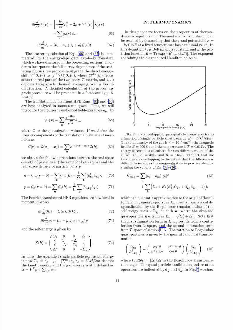
FIG. 7. Two overlapping quasi-particle energy spectra asa function of single-particle kinetic energy E = h2k2/(2m).The total density of the gas is n = 1014 cm−3, the magneticfield is B = 900 G, and the temperature is T = 0.01T F . Theenergy-spectrum is calculated for two different values of thecutoff: i.e. K = 32kF and K = 64kF . The fact that thetwo lines are overlapping to the extent that the difference isdifficult to see shows the renormalization in practice, demon-strating the validity of Eq. (32)-(36).

H diag =

i

(ν i − µm)|φi|2 (75)

+k

Σk + E k

α†k↑α

k↑ + α†k↓α

k↓ − 1

,

which is a quadratic approximation to the original Hamil-tonian. The energy spectrum E k results from a local di-agonalization by the Bogoliubov transformation of theself-energy matrix Σk at each k, where the obtained

quasi-particle spectrum is E k =

Σ2k + ∆2. Note that

the first summation term in H diag results from a contri-bution from Q space, and the second summation term

from P space of section II A. The rotation to Bogoliubovquasi-particles is given by the general canonical transfor-mation

αk↑

α†−k↓

=

cos θ −eiγ sin θ

eiγ sin θ cos θ

ak↑

a†−k↓

, (76)

where tan 2θk = |∆|/Σk is the Bogoliubov transforma-tion angle. The quasi-particle annihilation and creation

operators are indicated by αk

and α†k

. In Fig. 7 we show

11



a typical quasi-particle energy spectrum for 6Li versusthe single-particle kinetic energy, at a magnetic field of B = 900 G and a temperature of T = 0.01T F . Thefigure demonstrates how well the renormalizing equa-tions (32)-(36) work in obtaining a cutoff independentenergy spectrum. This is important because it impliesthat all the thermodynamics which follow will also beK -independent.

For the stationary solution the grand potential, orequivalently, the free energy, has indeed a minimum.This follows easily from setting the partial derivativeof the grand potential with respect to φi to zero:∂ ΦG/∂φi = 0. This gives the solution

φi = − gi p

ν i − µm

, (77)

which is also the stationary solution of Eq. (67). Thisequality is very useful because we can effectively elimi-nate the molecular field from the equations. The quasi-particle states are now populated according to the Fermi-Dirac distribution nk = [exp(E k/kbT ) + 1 ]−1. The mean

fields are then determined by integrating the equilibriumsingle particle density matrix elements, given by

n =1

(2π)2

K

0

dk

(2nk − 1)cos2θk + 1

, (78)

p =1

(2π)2

K

0

dk (2nk − 1)sin2θk , (79)

Since θk depends on n and p, these equations require self-consistent solutions which are found from a numericaliterative method.

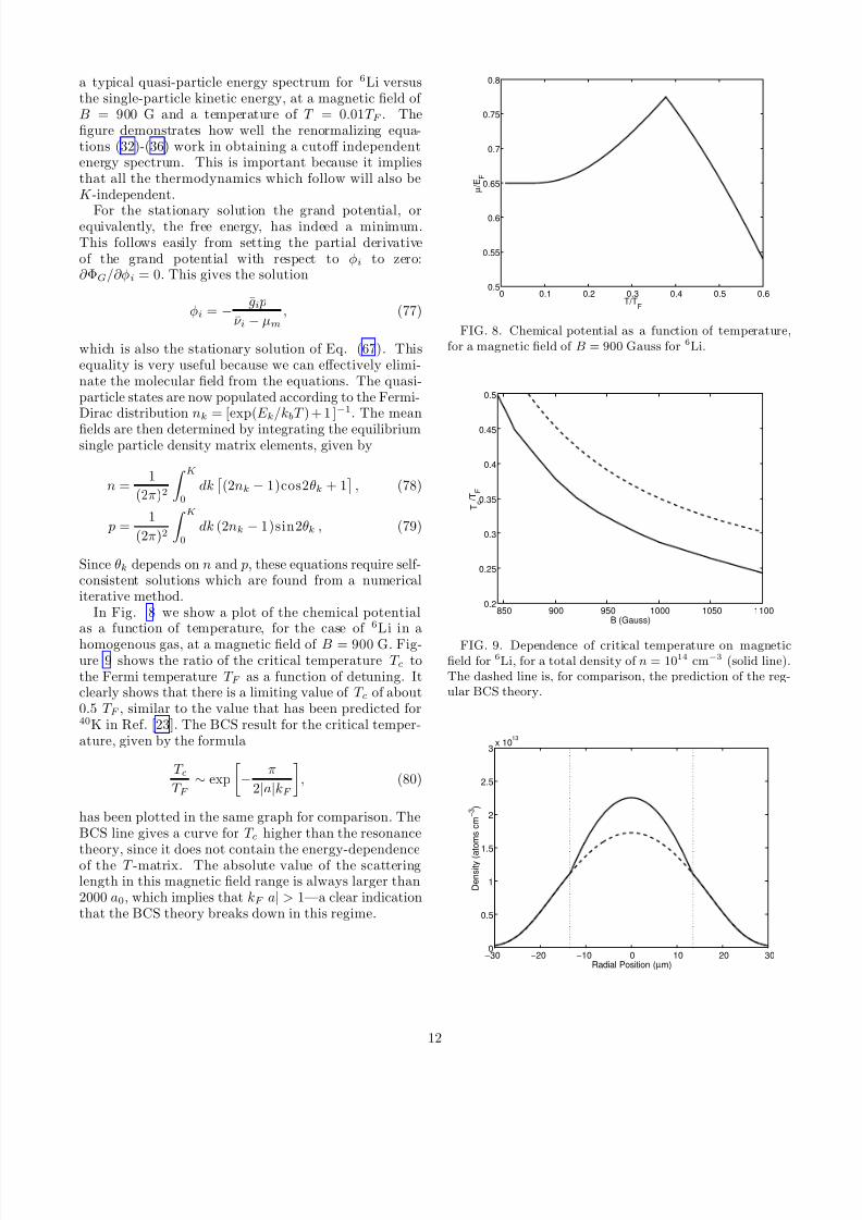
In Fig. 8 we show a plot of the chemical potentialas a function of temperature, for the case of 6Li in a

homogenous gas, at a magnetic field of B = 900 G. Fig-ure 9 shows the ratio of the critical temperature T c tothe Fermi temperature T F as a function of detuning. Itclearly shows that there is a limiting value of T c of about0.5 T F , similar to the value that has been predicted for40K in Ref. [23]. The BCS result for the critical temper-ature, given by the formula

T cT F

∼ exp

− π

2|a|kF

, (80)

has been plotted in the same graph for comparison. TheBCS line gives a curve for T c higher than the resonance

theory, since it does not contain the energy-dependenceof the T -matrix. The absolute value of the scatteringlength in this magnetic field range is always larger than2000 a0, which implies that kF |a| > 1—a clear indicationthat the BCS theory breaks down in this regime.

0 0.1 0.2 0.3 0.4 0.5 0.60.5

0.55

0.6

0.65

0.7

0.75

0.8

T/TF

µ / E F

FIG. 8. Chemical potential as a function of temperature,for a magnetic field of B = 900 Gauss for 6Li.

850 900 950 1000 1050 11000.2

0.25

0.3

0.35

0.4

0.45

0.5

B (Gauss)

T c

/ T F

FIG. 9. Dependence of critical temperature on magneticfield for 6Li, for a total density of n = 1014 cm−3 (solid line).The dashed line is, for comparison, the prediction of the reg-ular BCS theory.

−30 −20 −10 0 10 20 300

0.5

1

1.5

2

2.5

3x 10

13

Radial Position (µm)

D e n s i t y ( a

t o m s c m − 3 )

12



FIG. 10. Density profile for a gas of 6Li atoms (solid line),evenly distributed among the two lowest hyperfine states. Thetemperature is T = 0.2T F at a magnetic field of B = 900 G.The trap-constant is ω = 2π500 s−1, and we have a totalnumber N = 5 × 105 atoms. We compare this with a pro-file resulting from the same µ (but for different total numberN ), where artificially no superfluid is present by setting thepairing field p equal to zero (dashed line).

So far, our calculation has been done for a homoge-neous gas. We will also present results for a trappedlithium gas in a harmonic oscillator potential V (r) witha total number of N = 5 × 105 atoms, similar to whatwe presented for 40K in Ref. [24]. We treat the inhomo-geneity by making use of the semiclassical local-densityapproximation, which involves mainly the replacementof the chemical potential by a spatially-dependent ver-sion µ(r) = µ−V (r). The thermodynamic equations forthe homogeneous system are then solved at each point inspace [24]. As a result, we obtain a spatially-dependentdensity distribution. At zero temperature, for a non-superfluid system, this gives the well-known Thomas-

Fermi solution. For a resonance system, however, a den-sity bulge appears in the center of the trap, which iscaused by a change in compressibility when a superfluidis present. This is shown in Figure 10, for a sphericaltrap with a trap-constant of ω = 2π500 s−1. This bulgeis a signature of superfluidity and could experimentallybe seen by fitting the density distribution in the outherwings to a non-resonant system, and thus obtaining anexcess density in the middle of the trap. For a discussionof the abrupt change in the compressibility see Ref. ??.

V. FLUCTUATIONS IN THE MEAN FIELDS

AND CROSS-OVER MODEL

In this section we make some comments on the connec-tion between the resonance superfluidity theory we havepresented and related mean-field approaches to discussthe cross-over of superconductivity from weak to strongcoupling. In the mean-field theory of BEC, most oftenreflected in the literature by the Gross-Pitaevskii equa-tion or finite temperature derivatives, a small parame-ter is derived to justify the application of the theory.This parameter,

√na3 [6], may be obtained from a study

of higher order corrections to the quasi-particle energyspectrum. It has been suggested that for a fermi sys-tem which exhibits superfluidity the small parameter isgiven by a power of kF a, and that the BCS theory breaksdown when this parameter approaches unity. However,the small parameter in the theory of resonance superflu-idity cannot be simply a function of the scattering lengthfor detunings close to resonance. This can already beseen from the energy-dependence of the T -matrix, whichshows that around the Fermi-energy, the T -matrix mayhave an absolute value much smaller than at zero en-ergy where the scattering length is defined. Moreover,

even right on resonance when ν = 0 and the scatteringlength passes through infinity, the T -matrix remains wellbehaved.

Instead of calculating the small parameter of this sys-tem, we choose a different approach based on cross-overmodels between BCS and BEC, formulated by Nozieres[33], and later expanded upon by Randeria [34]. Inthe regular BCS theory for weakly coupled systems the

value of the critical temperature is given by the expo-nential dependence in Eq. (80), but for strongly coupledsystems this model results in a logarithmically diver-gent prediction for T c. The parameter (kF a)−1 is usu-ally taken to describe the crossover from the weak cou-pling Bose limit((kF a)−1 →−∞) to the strong coupling((kF a)−1 → +∞) BEC limit. The unphysical divergencein T c occurs because the process which dominates thetransition in the weak coupling regime is the dissocia-tion of pairs of fermions. For a strongly coupled sys-tem, however, the fermions are so tightly bound thatthe wave functions of pairs of atoms begin to overlap,and the onset of coherence is signaled by excitations of the condensed state, which occurs at a temperature wellbelow the dissociation temperature of the Cooper pairs.Thus, when moving from weak to strong coupling, thenature of the transition changes from a BCS to a BECtype mechanism. An explicit inclusion of the process of molecule formation, characterized by the detuning, res-onance width, and resonance position, will allow us tomove from one regime to the other.

The lowest order correction which connects betweenBCS and BEC type superconductivity can be made byaugmenting the density equation to account for the for-mation of pairs of atoms. This is done by using the ther-modynamic number equation N = −∂ ΦG

∂µ, with ΦG the

total thermodynamic grand potential

ΦG = Φ0G − kbT Σq,iql lnΓ(q, iql). (81)

The term Φ0G is a grand potential that does not include

the quasi-bound molecules and results from regular BCStheory. Retaining only this term yields a theory whichcan only account for the free and scattered fermionicatoms which contribute to the fermion density, thereforethe theory breaks down if a sizeable number of boundstates are formed. In the extreme limit of strong cou-pling, Φ0

G becomes negligible and equation (81) just re-duces to the thermodynamic potential of an ideal Bosegas. In this regime, the theory predicts the formation

of a condensate of molecules below the BEC transitiontemperature.The function Γ(q, iql), which is a function of momen-

tum q and thermal frequencies iql, is mostly negligible fora weakly coupled system and has little affect on the valueof T c in this regime. It allows for the inclusion of the low-est contributing order of quantum fluctuations [33,34] bymeans of a general inclusion of mechanisms for molecularpair-formation. In the resonance superfluidity model, asimilar term is present due to the formation of bosonic

13



molecular bound states φi, and prevents the critical tem-perature from diverging. When the coupling increases,the formation of molecules adds significantly to the totaldensity equation in both the cross-over models of super-conductivity and in the theory we have presented here.Moreover, the inclusion of the molecular term allows fora smooth interpolation between the BCS and BEC lim-its. This is clearly a substantial topic in its own right,

and will be addressed further in a future publication [35].

VI. CONCLUSIONS

We have shown that it is possible to derive a mean-fieldtheory of resonance superfluidity, which can be applied toultra-cold Fermi gases such as 6Li and 40K. The Hamilto-nian we use treats the resonant states explicitly, and au-tomatically builds the coupled scattering equations intothe many-body theory. With a study of analytical scat-tering we have shown that these scattering equations cancompletely reproduce a full coupled channels calculation

for the relevant energy regime. The energy-dependenceof the s-wave phase shifts can be described by a smallset of parameters which correspond to physical proper-ties, such as the non-resonant background value of thescattering length, and the widths and detunings of theFeshbach resonances. Close to resonance, we predict alarge relative value of 0.5 T F for the critical tempera-ture. The particular resonance under study for 6Li oc-curs in the (1/2, 1/2)+(1/2,−1/2) collision channel, andhas its peak at B0 = 844 G, and a width of about∆B ≈ 185 G [10,11]. This large width translates intoa large magnetic field range where the critical tempera-ture is within a factor of two from its peak value. Thisrange is, for comparison, much larger than for 40K. For6Li there are also two other Feshbach resonances, one inthe (1/2,−1/2) + (3/2,−3/2) state and another in the(1/2, 1/2)+(3/2,−3/2) state. They result from couplingto the same singlet bound state, and occur at field val-ues of about B0 = 823 G and B0 = 705 G, and have asimilar width to the (1/2, 1/2)+ (1/2,−1/2) resonance.The disadvantage of these resonances, however, is thatthe atoms in these channels suffer from dipolar losses,which are also resonantly enhanced. Three-body inter-actions will be largely suppressed, as asymptotic p-wavecollisions will give very little contribution in the tem-perature regime considered (an s-wave collision is alwaysforbidden for at least one of the pairs). From a study

of cross-over models between BCS and BEC we find noindication of break-down effects of the applied mean-fieldtheory.

ACKNOWLEDGEMENTS

We thank J. Cooper, E. Cornell, D. Jin, C. Wieman,B.J. Verhaar and B. DeMarco for very stimulating dis-

cussions. Support is acknowledged for S.K. and J.M.from the U.S. Department of Energy, Office of BasicEnergy Sciences via the Chemical Sciences, Geosciencesand Biosciences Division, and for M.C. from SNS, Pisa(Italy). Support is acknowledged for M.H. and M.C. fromthe National Science Foundation, and for R.W. from theAPART fellowship, Austrian Academy of Sciences.

[1] M. H. Anderson, J. R. Ensher, M. R. Matthews, C. E.Wieman, and E. A. Cornell, Science 269, 198 (1995);K. B. Davis, M.-O. Mewes, M. R. Andrews, N. J. vanDruten, D. S. Durfee, D. M. Kurn, and W. Ketterle,Phys. Rev. Lett. 75, 3969 (1995); C. C. Bradley, C. A.Sackett, J. J. Tollett, and R. G. Hulet, Phys. Rev. Lett.75, 1687 (1995); 79, 1170(E) (1997).

[2] J.E. Williams and M.J. Holland, Nature (London) 401,568 (1999); M.R. Matthews, B. P. Anderson, P.C. Hal-

jan, D.S. Hall, C.E. Wieman, and E. A. Cornell M.R.Matthews et al., Phys. Rev. Lett. 83, 2498 (1999); K.W.Madison, F. Chevy, W. Wohlleben, and J. Dalibard,Phys. Rev. Lett. 84, 806 (2000), P.C. Haljan, I. Cod-dington, P. Engels, and E.A. Cornell, Phys. Rev. Lett.87, 210403 (2001), J.R. Abo-Shaeer, C. Raman, J.M.Vogels, and W. Ketterle, Science 292, 476 (2001).

[3] B. DeMarco and D. S. Jin, Science 285, 1703 (1999).[4] G. Truscott, K. E. Strecker, W. I. McAlexander, G. B.

Partridge, and R. G. Hulet, Science 291, 2570 (2001).[5] F. Schreck, L. Khaykovich, K. L. Corwin, G. Ferrari, T.

Bourdel, J. Cubizolles, and C. Salomon, Phys. Rev. Lett.87, 080403 (2001).

[6] S.T. Beliaev, Sov. Phys. JETP 34, 323 (1958).

[7] A.A. Abrikosov, L.P. Gorkov, and I.E. Dzyaloshinski,Methods of Quantum Field Theory in Statistical Physics,Prentice-Hall Inc., New Jersey, (1963);

[8] H. Feshbach, Ann. Phys. 5, 357 (1958); ibid., Ann. Phys.19, 287 (1962), H. Feshbach, Theoretical Nuclear Physics,(Wiley, New York, 1992).

[9] E. Tiesinga, B. J. Verhaar, and H. T. C. Stoof, Phys.Rev. A 47, 4114 (1993)

[10] S. Kokkelmans and B.J. Verhaar, (private communica-tion). The calculation is based on the analysis of thelithium interactions as described in [11]. An alternativeanalysis has been described in [12].

[11] F. A. van Abeelen, B. J. Verhaar, and A. J. Moerdijk,Phys. Rev. A 55, 4377 (1997).

[12] E. R. I. Abraham et al., Phys. Rev. A 55, R3299 (1997).[13] H.T.C. Stoof, J.M.V.A. Koelman, and B.J. Verhaar,

Phys. Rev. B 38, 4688 (1988).[14] J. Bardeen, L. N. Cooper, and J. R. Schrieffer, Phys.

Rev. 108, 1175 (1957); J. R. Schrieffer, Theory of Su-

perconductivity , Perseus Books, Reading, Massachusetts,(1999).

[15] A. G. Leggett, J. Phys. (Paris) C7, 19 (1980); M. Hou-biers and H. T. C. Stoof, Phys. Rev. A 59, 1556-1561(1999); G. Bruun, Y. Castin, R. Dum et al., Eur. Phys.

14



J. D 7, 433–439 (1999); H. Heiselberg, C. J. Pethick, H.Smith, and L. Viverit, Phys. Rev. Lett. 85, 2418 (2000).

[16] J.R. Taylor, Scattering Theory , (Wiley, New York, 1972).[17] A.J. Moerdijk, B.J. Verhaar, and A. Axelsson, Phys. Rev.

A 51, 4852 (1995).[18] S.J.J.M.F. Kokkelmans, B.J. Verhaar, and K. Gibble,

Phys. Rev. Lett. 81, 951 (1998).[19] P.J Leo, E. Tiesinga, P.S. Julienne, Phys. Rev. Lett. 81,

1389 (1998)[20] E.G.M. van Kempen, S.J.J.M.F. Kokkelmans, D.J.

Heinzen, and B.J. Verhaar, to be published in Phys. Rev.Lett.

[21] M. Houbiers, H.T.C. Stoof, W.I. McAlexander, and R.G.Hulet, Phys. Rev. A 57, R1497 (1998).

[22] J.M. Vogels, B.J. Verhaar, and R.H. Blok, Phys. Rev. A57, 4049 (1998).

[23] M. Holland, S.J.J.M.F. Kokkelmans, M.L. Chiofalo, andR. Walser, Phys. Rev. Lett. 87, 120406 (2001).

[24] M.L. Chiofalo, S.J.J.M.F. Kokkelmans, J.N. Milstein,and M. Holland, submitted to Phys. Rev. Lett.

[25] A. I. Akhiezer and S. V. Peletminskii, Methods of Sta-

tistical Physics, Pergamon Press Ltd., Oxford, England(1981).

[26] R. Walser, J. Williams, J. Cooper, M. Holland, Phys.Rev. A. 59, 3878 (1999).

[27] R. Walser and J. Cooper and M. Holland, Phys. Rev. A63, 013607 (2001).

[28] E. Timmermans et al., Phys. Rev. Lett. 83, 2691 (1999).[29] F.A. van Abeelen and B.J. Verhaar, Phys. Rev. Lett. 83,

1550 (1999).[30] M. Holland, J. Park, and R. Walser, Phys. Rev. Lett. 86,

1915 (2001)[31] S.J.J.M.F. Kokkelmans, H. M. J. Vissers, and B. J. Ver-

haar, Phys. Rev. A 63, 031601 (2001).[32] J. P. Blaizot and G. Ripka, Quantum Theory of Fi-

nite Systems, The MIT Press, Cambridge, Massachusetts

(1986).[33] P. Nozieres and S. Schmitt-Rink, J. Low Temp. Phys. 59,195 (1982).

[34] See M. Randeria in Bose-Einstein condensation , ed. byA. Griffin, D.W. Snoke and S. Stringari, Cambridge Un.Press, Cambridge (1995).

[35] J.N. Milstein, S.J.J.M.F. Kokkelmans, R. Walser, andM.J. Holland, to be published.

15

S.J.J.M.F. Kokkelmans et al- Resonance Superfluidity: Renormalization of Resonance Scattering Theory

Documents