Size Distortions of Tests of the Null Hypothesis of ...fordschool.umich.edu/rsie/workingpapers/Papers426-450/r444.pdfSize Distortions of Tests of the Null Hypothesis of Stationarity:

RESEARCH SEMINAR IN INTERNATIONAL ECONOMICS

School of Public PolicyThe University of Michigan

Ann Arbor, Michigan 48109-1220

Discussion Paper No. 444

Size Distortions ofTests of the Null Hypothesis of Stationarity:

Evidence and Implications for the PPP Debate

Mehmet CanerBilkent University

and

Lutz KilianUniversity of Michigan

July 30, 1999

Recent RSIE Discussion Papers are available on the World Wide Web at:http://www.spp.umich.edu/rsie/workingpapers/wp.html

2

Size Distortions of

Tests of the Null Hypothesis of Stationarity:

Evidence and Implications for the PPP Debate

Mehmet Caner Lutz KilianBilkent University University of Michigan

and CEPR

July 30, 1999

Abstract: Tests of the null hypothesis of stationarity against the unit root alternative play anincreasingly important role in empirical work in macroeconomics and in international finance.We show that the use of conventional asymptotic critical values for stationarity tests may causeextreme size distortions, if the model under the null hypothesis is highly persistent. This factcalls into question the use of these tests in empirical work. We illustrate the practical importanceof this point for tests of long-run purchasing power parity under the recent float. We show thatthe common practice of viewing tests of stationarity as complementary to tests of the unit rootnull will tend to result in contradictions and in spurious rejections of long-run PPP. While thesize distortions may be overcome by the use of finite-sample critical values, the resulting teststend to have low power under economically plausible assumptions about the half-life ofdeviations from PPP. Thus, the fact that stationarity is not rejected cannot be interpreted asconvincing evidence in favor of mean reversion. Only in the rare case that stationarity is rejecteddo size-corrected tests shed light on the question of long-run PPP.

KEY WORDS: Long-run PPP; mean reversion; finite-sample critical values; real exchange rates.

Acknowledgments: We thank Bob Barsky, Bruce Hansen, Bart Hobijn, Jan Kmenta, SteveLeybourne, David Papell and Shaowen Wu for helpful discussions. An earlier version of thispaper circulated under the title “Size Distortions of Tests of the Null Hypothesis of Stationarity:Evidence and Implications for Applied Work”.

Correspondence to: Lutz Kilian, Department of Economics, University of Michigan, Ann Arbor,MI 48109-1220. Fax: (734) 764-2769. Phone: (734) 764-2320. Email: [email protected]

3

1. Introduction

Recently, there has been increasing interest in tests of the null hypothesis of a level stationary

process (or more precisely I(0) process) against the alternative of a difference stationary (or I(1))

process. These tests are widely used in empirical macroeconomics and in international finance

both in their own right and as complements to more traditional tests of the unit root null

hypothesis (see, for example, Choi (1994), Lewbel (1996), Culver and Papell (1997, 1999), Lee

et al. (1997), Collins and Anderson (1998), Wolters et al. (1998), Kuo and Mikkola (1999)).1

We show that there are serious problems with the interpretation of these tests in practice that

applied users need to be aware of and that are of immediate relevance for many questions in

international finance, including tests of long-run purchasing power parity (PPP).

The two most widely used tests of the I(0) null hypothesis are due to Kwiatkowski et al.

(1992), henceforth KPSS test, and to Leybourne and McCabe (1994), henceforth LMC test.

Asymptotic critical values for both tests are given in Kwiatkowski et al. (1992). However, these

critical values make no distinction between a process that is white noise and a highly persistent

stationary process. We provide new evidence that in models with roots close to unity the use of

asymptotic critical values may cause extreme size distortions. The existence of such size

distortions has not been documented in the previous literature. While Kwiatkowski et al. report

some size results for the KPSS test, their data generating processes are of relevance mainly for

annual data. Leybourne and McCabe (1994) report low size distortions for the Leybourne and

McCabe test in a somewhat more realistic setting, but their favorable simulation results appear to

be due to a programming error. In contrast, we provide a comprehensive analysis of the size of

both the KPSS test and the LMC test for the regions in the parameter space that are relevant for

typical quarterly and monthly processes.

4

Our findings of severe size distortions are of immediate practical interest. It is well

known that the processes of interest in empirical macroeconomics and in international finance

tend to be highly persistent even under the null of stationarity (see Rudebusch, 1993; Diebold and

Senhadji, 1996; Lothian and Taylor, 1996). Since for such processes the KPSS and LMC test

have a tendency to reject the null of stationarity whether it is true or not, we conclude that it is all

but impossible to interpret rejections of the stationarity hypothesis in empirical work.

This fact also has important implications for the common practice of testing both the null

hypothesis of a unit root and that of stationarity. Evidence against the stationarity null, but not

the unit root null is typically interpreted as conclusive evidence that the underlying process is

difference stationary (see, for example, Baillie and Pecchenino (1991), Cheung and Chinn

(1997), Ely and Robinson (1997), Moreno (1998)). Our results imply that applied users will tend

to spuriously accept the difference stationary model in practice, given the low power of unit root

tests. Rejections of stationarity in favor of a unit root process are indeed common in applied

work. Moreover, size distortions of stationarity tests may generate contradictory test results with

both null hypotheses being rejected.

We illustrate the practical importance of this point for tests of long-run PPP in the post-

Bretton Woods period. Our empirical analysis extends recent work by Culver and Papell (1999)

who applied the KPSS test to quarterly data under the recent float. We use both the KPSS and

the LMC test, and we include monthly real exchange rate data in our analysis. We find that both

tests are likely to overstate the evidence against long-run PPP under the recent float. Notably the

LMC test rejects the null of stationarity for virtually all countries in favor of a unit root process.

An important question is to what extent the size distortions of stationarity tests may be

mitigated by replacing the asymptotic critical values by size-adjusted finite-sample critical

5

values. Recently, such corrections have been employed by Cheung and Chinn (1997), Rothman

(1997) and Kuo and Mikkola (1999), among others. We derive size-corrected critical values for

the LMC and KPSS test under economically plausible assumptions about the half-life of

deviations from PPP. Using size-adjusted critical values for the KPSS and LMC test instead of

asymptotic critical values, we are unable to reject the stationarity null for any country but Japan.

However, this sharp reversal in results cannot be interpreted as convincing evidence in

favor of long-run PPP. We show that after size corrections the power of the KPSS (LMC) test

falls as low as 20 % (22 %) at the 5 % level for the sample sizes and degrees of persistence of

interest in the PPP literature. This means that tests based on size-adjusted critical values are

unlikely to reject stationarity whether long run PPP holds or not. Thus, we learn very little from

conducting tests with size-corrected critical values except in the rare case of a rejection of

stationarity. Our example of the problems with interpreting results of stationarity tests is

representative for a wide range of applications in macroeconomics and international finance. We

conclude that these tests should not be used without size-adjusting the critical values and will

tend to be of limited usefulness even with size-adjustments unless the sample size is very large.

In section 2, we review the construction of the KPSS and LMC tests of stationarity. In

section 3 we document the size distortions of the KPSS and LMC tests based on asymptotic

critical values. In section 4, we illustrate the practical importance of the size distortions for

applied work in the context of the PPP debate. In section 5, we analyze the size-corrected power

of the LMC and KPSS tests and reexamine the empirical findings. Section 6 concludes.

2. A Review of the Two Leading Examples of Tests of Stationarity

The two most widely used tests of the I(0) null hypothesis are due to Kwiatkowski et al. (1992)

and to Leybourne and McCabe (1994). These two tests differ in how they account for serial

6

correlation under H0 . Whereas the KPSS test uses a nonparametric correction similar to the

Phillips-Perron test, the LMC test allows for additional autoregressive lags similar to the

augmented Dickey-Fuller (ADF) test. Although both tests have the same asymptotic distribution,

the LMC test statistic converges at rate O TP ( ) compared to a rate of only O T lP ( / ) for the

KPSS statistic where l is the autocorrelation truncation lag. Moreover, the LMC test is robust to

the choice of lag order, whereas the KPSS test can be sensitive to the choice of l (see Leybourne

and McCabe (1994), Lee (1996)).

2.1. Leybourne-McCabe Test

Following Leybourne and McCabe (1994), we consider the generalized local levels model

Φ( )L y tt t t= + +α β ε (1)

and

α α ηt t t= +−1 , α α0 = , t T= 1, ... , , (2)

where Φ( ) ...L L L Lpp= − − − −1 1 2

2φ φ φ is a pth-order autoregressive polynomial in the lag

operator L with roots outside the unit circle. We assume that ε t is distributed iid ( , )0 2σ ε andηt is

distributed iid ( , )0 2σ η . We also assume that ε t andηt are mutually independent. Under

regularity conditions, the structural model (1) and (2) can be shown to be second-order

equivalent in moments to the ARIMA(p,1,1) reduced form process:

Φ( ) ( ) ( )L L y Lt t1 1− = + −β θ ζ , (3)

with suitably defined MA coefficient θ and iid innovations ζ t with distribution ( , )0 2σζ . It can

be shown that 0 1< <θ for 0 2< < ∞ση . This specification accounts for the presence of a nonzero

MA(1) component in the growth rates of many economic time series. A test of the null

7

hypothesis that yt follows a trend-stationary ARIMA(p,0,0) process against the alternative of an

ARIMA(p,1,1) model with positive MA coefficient can be stated as H02 0:ση = against

H12 0:ση > in the structural model with β ≠ 0 .

To implement the LMC test we construct the series:

y y yt t i t ii

p* *= − −

=∑φ

1

where the φi* are the maximum likelihood estimates of φi from the fitted ARIMA(p,1,1) model

∆ ∆y yt i t ii

p

t t= + + −−=

−∑β φ ζ θ ζ1

1 (4)

and then calculate the residuals from the least-squares regression of yt* on an intercept and

deterministic time trend. Denoting these residuals $ε t , the test is based on

$ $ $’ $s T Vβ εσ ε ε= − −2 2

where $ $’ $ /σ ε εε2 = T is a consistent estimator of σ ε

2 and V is a T x T matrix with ijth element

equal to the minimum of i and j. We reject the null hypothesis of stationarity if the test statistic

exceeds its critical value under H0 .

If β is known to be zero in population, the residuals $ε t are obtained from regressing yt*

on an intercept alone. The resulting test statistic is:

$ $ $’ $s T Vα εσ ε ε= − −2 2

Asymptotic critical values for both of these statistics are provided in Kwiatkowski et al. (1992).

We follow Leybourne and McCabe in programming the test in GAUSS. A key issue in the

implementation of the LMC test that is not discussed in their paper is the choice of starting

values for the ARIMA(p,1,1) model. Rather than rely on the standard optimization algorithm

8

used by the GAUSS-ARIMA routine, Leybourne and McCabe evaluate the likelihood function

for a grid of initial values for the moving average parameter, θ 0 , ranging from 0 to -1 in

increments of 0.05, with the initial value of the autoregressive parameter(s) fixed at θ 0 01− . . In

particular, for p = 1, the initial guess for the AR parameter is defined as φ θ10 0 01= − . . For p > 1,

the initial guess is φ φ θ10 0 0 01= = = −K p . . The starting value for the drift parameter is set equal

to 0.1. In this paper, we extend Leybourne and McCabe’s procedure by including among the

candidate models the model selected based on the default initial values supplied by the GAUSS-

ARIMA routine. The model that achieves the highest likelihood is selected for the final analysis.

The GAUSS code for our estimation procedure is available upon request.2

2.2. KPSS Test

The KPSS test of stationarity is based on the same model as the LMC test and has the same

general structure. The KPSS test statistic for the model with time trend is computed as

$ $ $’ $d T Vβ εσ ε ε= − −2 2 ,

where $εt is the least-squares residual from a regression of yt* on an intercept and deterministic

time trend. The difference to the LMC test is that the KPSS test relies on a nonparametric

estimator of the long-run variance of εt :

$ $ ’ $ ( , ) $ ’ $σ ε ε ε εε2

1

2= + −=∑t t t t ii

l

T w i l T ,

where w(i,l) = 1- i/(l+1) is the Bartlett kernel. This estimator is consistent if the truncation lag l

increases with the sample size at a suitable rate. We set l T= int[ ( / ) ]/12 100 1 4 where int

denotes the integer part (see Kwiatkowski et. al. (1992), Lee (1996)).3

Similarly, for β = 0, the residuals $ε t are obtained from regressing yt* on an intercept

9

alone. The resulting test statistic is:

$ $ $’ $d T Vα εσ ε ε= − −2 2 ,

where $σε2 is defined as before. The asymptotic critical values for these statistics are identical to

those for the LMC test.

3. Evidence of Size Distortions

This is not the first paper to examine the size of tests of stationarity. For example, Kwiatkowski

et al. (1992) and Lee (1996) have provided size results for a range of sample sizes and values of

ρ. However, their results are limited to the AR(1) model with slope parameter ρ ≤ 0 8. .

Kwiatkowski et. al. make the case that “ρ = 0 8. is a plausible parameter value since, if we take

most series to be stationary, their first-order autocorrelations will often be in this range” (p.

171/172). This view may be plausible for some of the annual Nelson and Plosser (1982) data

analyzed in Kwiatkowski et al., but it is highly unrealistic for most monthly and quarterly data.

In this paper, we make the case that many econometric applications of stationarity tests

involve processes with roots much closer to unity (see Rudebusch (1993), Cheung and Chinn

(1997)). While Leybourne and McCabe (1994) provide some additional small-sample evidence

for the size of the LMC and KPSS tests, the low size distortions they find for the LMC test

appear to be due to a programming error. Moreover, their evidence is limited to processes with

roots between 0 and 0.9. As we will show, there is reason to expect the dominant root of many

stationary processes to be closer to 0.94-0.99 in practice. Thus, the relevant models from an

economic point of view are a highly persistent process under the null of stationarity and a unit

root process under the alternative. There is reason to doubt the finite-sample accuracy of the

asymptotic critical values for such highly persistent processes.4 We illustrate this point by

10

extending the simulation evidence for the KPSS test and the LMC test to processes with larger

roots. We use the critical values compiled by Kwiatkowski et al. (1992) and used in most

applied work.5

The size of the KPSS test is highly sensitive to the choice of the truncation lag l. We

therefore follow the recommendation of Kwiatkowski et al. (1992) and Lee (1996) and choose a

comparatively large value of l such that l T= int[ ( / ) ]/12 100 1 4 . This choice tended to produce

the most accurate test results in previous studies. For the LMC test we set p = 1, since the size

of the test is not sensitive to the lag order used. The data generating process is an AR(1) process

with root ρ and NID(0,1) innovations. The sample size is T ∈{100, 300, 600}. Table 1 shows

the effective size of both the KPSS and the LMC test. Results for the model without trend are

shown in Table 1a and those for the model with trend in Table 1b. We focus on the nominal 5 %

test. Qualitatively similar results are obtained at the nominal 10 % level.

Table 1a shows the rejection rate under the null hypothesis for a range of values of ρ

from 0 to 0.99. It is evident that the size distortions for roots near unity are large and increasing,

unlike the size results reported in Kwiatkowski et al. (1992), Lee (1996) and Leybourne and

McCabe (1994).6 For example, for ρ = 0.9 and T = 100, the rejection rate of the nominal 5 %

LMC test based on conventional asymptotic critical values is 32 %. For ρ = 0.99 and T = 100,

the rejection rate rises to 74 %. Even for T = 600, the rejection rate may be as high as 70 (45, 14,

9) % for ρ = 0.99 (0.98, 0.95, 0.9). Similarly, the KPSS test rejects the null hypothesis in up to

77 % of all trials. Based on this evidence, one would expect both tests to reject the null

hypothesis of stationarity far too often in small samples. Qualitatively similar results hold for the

11

model with trend in Table 1b.

It is of some practical interest to compare the performance of the LMC and the KPSS test.

For the model without trend, the KPSS test tends to be almost uniformly more accurate than the

LMC test for T = 100, for T = 300 the LMC test is more accurate, except for the most persistent

processes, and for T = 600 the LMC test is uniformly more accurate. The size of both tests

improves with larger sample size, but only very slowly. Consistent with the theoretical results

about the rate of convergence of the two tests, the size of the LMC test converges much more

rapidly to its nominal level than that of the KPSS test. However, for the relevant range of ρ ,

severe size distortions persist even for T = 600. For the model with trend in Table 1b, the size

distortions of the LMC test tend to be considerably smaller than in Table 1a. Except for T = 100,

the LMC test almost always is more accurate than the KPSS test, often by a wide margin. The

differences are most pronounced for larger sample sizes. However, even the LMC test has

rejection rates of up to 58 percent for ρ = 0.99 and T = 300.

Table 1 also shows that for highly persistent stationary processes, the convergence of the

size to its nominal level may be non-monotonic. As the sample size increases from T = 100 to T

= 300, the effective size actually worsens in some cases. For T = 600, the effective size

improves relative to T = 300, but may still be higher than for T = 100. The degree of non-

monotonicity is more pronounced for the KPSS test than for the LMC test.

We conclude that both tests have a strong tendency to spuriously reject the null

hypothesis of stationarity for realistic values of ρ and T. The existence of such severe size

distortions has not been previously documented in the literature. In applied work, rejections of

the stationarity hypothesis based on asymptotic critical values have often been welcomed as

strong evidence in favor of a unit root (and as a formal justification for pursuing cointegration

12

tests for linear combinations of I(1) variables). Our results suggest that many of these findings

are likely to have been spurious.

4. Example: Testing for Long-Run PPP in the Post-Bretton Woods Era

4.1. Motivation

More than twenty years after the breakdown of the Bretton Woods exchange rate system there

still is considerable disagreement over the question of whether real exchange rates are mean-

reverting (see Froot and Rogoff, 1995; Rogoff, 1996). While most economists find some version

of long-run purchasing power parity plausible and indeed well nigh indispensable in the

construction of theoretical international macroeconomic models, statistical tests for the absence

of mean reversion to date have yielded at best conflicting results. This makes it appealing to test

directly the null hypothesis that real exchange rates are mean-reverting. A failure to reject this

null hypothesis would not suffice to convince a skeptic of the existence of long-run PPP, but a

rejection would be compelling evidence against long-run PPP. Such PPP tests have been

conducted for example by Baillie and Pecchenino (1991) to assess the validity of the building

blocks of the monetary model of exchange rate determination for the U.K. and the U.S. Kuo and

Mikkola (1999) conduct a similar analysis for long-run US-UK real exchange rates. However,

their analysis has no direct implications for the post-Bretton Woods period. In work more

closely related to ours, Culver and Papell (1999) observe that the failure to reject the null of

stationarity for real exchange rates, together with evidence against the null of stationarity for

nominal exchange rates for the same sample period, would constitute strong evidence of long-run

PPP. Culver and Papell investigate the null hypothesis of stationary real exchange rates in the

post-Bretton Woods era using the KPSS test. For quarterly real exchange rate data, they

conclude that the evidence against long-run PPP is mixed, with the KPSS test at the 5 percent

13

critical value not rejecting the null of stationarity in most cases.

What makes the application of stationarity tests to real exchange rates problematic is the

fact that the mean-reversion in real exchange rates is slow. Slow mean reversion does not

contradict the view that long-run PPP holds. It is well known that theoretical models with

intertemporal smoothing of consumption goods (see Rogoff, 1992) or cross-country wealth

redistribution effects (see Obstfeld and Rogoff, 1995) imply highly persistent but transitory

deviations from PPP. Thus, the relevant comparison involves a highly persistent stationary null

and a unit root alternative, consistent with our claim in section 3. One would expect that the

accuracy of the test depends on the value of the dominant root under the null hypothesis. Since

the extent of the size distortions increases with the persistence of the process under the null

hypothesis, it is essential to obtain a sense of the degree of mean reversion under the null in order

to assess the potential size distortions in applied work. It is useful to reparameterize this problem

in terms of the half-life of the response of the real exchange rate to a shock.

There is a consensus view in the PPP literature about the half-life of the response of the

real exchange rate to a shock. For example, Abuaf and Jorion (1990, p. 173) suggest a half-life

of 3-5 years for the post-Bretton Woods era. Rogoff (1996, pp. 657-658) conjectures that

deviations from PPP dampen out at the rate of about 15 percent per year. Froot and Rogoff

(1995), p. 1645) consider a half-life of 3-5 years quite plausible. Recently, this consensus has

been reaffirmed by Murray and Papell (1999). In what follows, we will exploit the close link

between the half-life and the value of the autoregressive root in an AR(1) model, ρ , to obtain a

benchmark for plausible values of ρ . The half-life of the response of the process to a shock is

defined as h = i/f where f denotes the sampling frequency of the data (1/year for years; 4/year for

quarters; 12/year for months, etc.) and i is defined by ρ i = 05. . Under H0 , the value of the root

14

ρ of the AR(1) model:

y yt t t= + +−α ρ ε1 , (5)

is a function of the half-life. For example, if the half-life of an innovation is 5 years under H0

and the data frequency is monthly, ρ = =0 5 0 98851 60. .( / ) . For quarterly data, under the same

assumptions, ρ = =0 5 1 20. ( / ) 0 9659. , and for annual data ρ = =05 0 87041 5. .( / ) . For the null

hypothesis of a half-life of three years, the corresponding values are ρ = =05 0 98091 36. .( / ) for

monthly data, ρ = =05 0 94391 12. .( / ) for quarterly data, and ρ = =05 0 79371 3. .( / ) for annual data.

Thus, to the extent that the real exchange rate is well approximated by an AR(1) process,

the simulation results in Table 1a suggest that the LMC test will reject the I(0) null with about 70

percent probability for monthly and about 55 percent probability for quarterly data, if real

exchange rates indeed are stationary with half-lives of about 3-5 years. For the KPSS test the

corresponding rejection rates are about 60 percent for the monthly data and 30 percent for the

quarterly data. Thus, it seems all but impossible to determine in practice whether the test

correctly rejects the null in favor of a unit root or whether the rejection is simply due to size

distortions. We will illustrate this point in the next section.

4.2. Empirical Analysis

The real exchange rate data are constructed from the IMF’s International Financial Statistics

data base on CD-ROM. They are based on the end-of-period nominal U.S. dollar spot exchange

rates and the U.S. and foreign consumer price indices. The first data set comprises monthly data

for 1973.1-1997.4 (292) observations for 17 countries including Austria, Belgium, Canada,

Denmark, Finland, France, Germany, Greece, Italy, Japan, The Netherlands, Norway, Portugal,

15

Spain, Sweden, Switzerland, and the United Kingdom. The second data set includes quarterly

data for 1973.I-1997.II (98 observations) for the same 17 countries plus Australia, Ireland, and

New Zealand.

We begin the analysis with the LMC test of the null hypothesis of stationarity. The lag

orders for the ARIMA(p,1,1) model were selected using the Akaike Information Criterion (AIC).

Our results are robust to alternative assumptions about the lag order. Table 2 provides strong

evidence against the null hypothesis of PPP for all countries at the monthly frequency and for all

countries but Australia, New Zealand and Switzerland at the quarterly frequency. The apparent

finding of a unit root in all 17 monthly and 17 of the 20 quarterly series is striking in that no

other test to date has produced such strong results. If correct, these results would imply that

most, if not all, real exchange rate processes contain important permanent components, implying

a sharp reversal of the evidence in the literature and a direct rejection of long-run PPP.

It would be tempting to rationalize this result by appealing to theoretical explanations

such as permanent changes in the relative productivity of the tradables and nontradables sector

(see Baumol and Bowen, 1966), permanent changes in the level of government spending (see

Froot and Rogoff, 1991; Alesina and Perotti, 1995), and systematic bias in CPI measurement (see

Shapiro and Wilcox, 1996). However, we know from Table 1 that such strong rejections are

extremely likely a priori, even if the null hypothesis is true. Thus, the results of the LMC test are

not informative. We cannot tell whether the test correctly rejects the null in favor of a unit root

or whether the rejection is simply due to size distortions. Moreover, this problem is unlikely to

be overcome by waiting for more data to accumulate. The size results in Table 1a suggest that

even doubling the sample size for the monthly real exchange rate to about 600 observations

would do little to improve the accuracy of the test.

16

The second column of Table 2 shows the corresponding results for the KPSS test. Recall

that our size results in Table 1a suggested that the KPSS test will tend to have lower size

distortions than the LMC test for the sample sizes and degrees of persistence of relevance to the

PPP debate. This fact is consistent with the observation that in Table 2 there are far fewer

rejections for the KPSS test than for the LMC test. However, the number of rejections using the

KPSS test is smaller (and that of the LMC test larger) than suggested by the simulation evidence.

It is interesting to compare our findings to the results of previous studies. For our choice

of l, Culver and Papell (1999) reject the null of stationarity at the quarterly frequency for

Australia, Ireland, and Japan.7 Using our updated sample, we obtain the same rejections for the

quarterly data plus Canada and Switzerland. In contrast, at the monthly frequency, the KPSS test

rejects the null of stationarity for 7 of 17 countries (Austria, Canada, Greece, Italy, Portugal,

Spain, Switzerland). This pattern is consistent with the evidence of increasing size distortions, as

ρ and T are increased, for both the LMC and KPSS test (see Table 1a).

As in the case of the LMC test, the observed rejections of the stationarity null by the

KPSS test are not informative, given the size distortions of the KPSS test based on asymptotic

critical values. It is quite possible that the observed rejections are spurious. This view is

supported by test results for the asymptotically efficient DF-GLS test of the unit root hypothesis.

We focus on this test because its power compares favorably to standard ADF tests (see Cheung

and Lai (1998), Elliott et al. (1996)). The DF-GLS test for the case of unknown mean is based on

the following regression:

( ) ( )1 10 11

− = + − +− −=

∑L y y L yt t j t j tj

pµ µ µφ φ ζ

where ytµ , the locally demeaned process under the local alternative of ρ = +1 c T/ , where

17

c < 0, is given by

y y zt t tµ β= − ,

with zt = 1 and β being the least-squares regression coefficient of ~yt on ~zt , the latter being

defined by ~ [ , ( ) , ..., ( ) ]’y y L y L yt T= − −1 21 1ρ ρ and ~ [ , ( ) , ..., ( ) ]’z z L z L zt T= − −1 21 1ρ ρ . The

DF-GLS test statistic is given by the t-ratio for testing H0 0 0: φ = against the one-sided

alternative H0 0 0: .φ < Implementation of the test requires the choice of the parameter c. We

follow Elliott et al.’s recommendation and set c = -7.

Rather than using the asymptotic critical values for the DF-GLS test we rely on

approximate finite-sample critical values. Finite-sample critical values under the unit root null

hypothesis may be obtained by simulation as described in Elliott et al. (1996). We depart from

that procedure in that we allow for some serial correlation under the null hypothesis. We

postulate an ARIMA(0,1,1) model, consistent with the assumptions of the LMC and KPSS tests,

withθ = 0.25. This specification accounts for the presence of a small nonzero MA(1)

component in the growth rates of many economic time series, including real exchange rates (see

Engel and Kim, 1998); Canzoneri et al., 1999; Froot and Rogoff, 1996; Lothian and Taylor,

1996). In fitting the ADF model and in calculating the finite sample critical values, we use

sequential t-tests with upper bounds of 8 autoregressive lags in the quarterly case and 12 lags in

the monthly case. Thus, our critical values allow for lag order uncertainty.

For the same data set, for which the LMC test (and to a lesser extent the KPSS test) find

strong evidence against stationarity, Table 2 shows that the 5 (10) percent DF-GLS test rejects

the unit root null hypothesis for (0) 3 of the 17 countries for which monthly data are available

and for 11 (15) of the 20 countries for which quarterly data are available.8 In fact, for several

18

countries the test results for the DF-GLS test directly contradict those for the stationarity tests.

For example, for Greece and Italy the KPSS test rejects stationarity at the monthly frequency, yet

the DF-GLS test rejects the unit root null hypothesis. No such contradictions occur at the

quarterly frequency. For the LMC test the contradictions are more numerous and include 3

countries for the monthly data and 14 countries for the quarterly data.

Of course, it is possible that some of these contradictions are driven by size distortions of

the DF-GLS test. Investigating that possibility would be beyond the scope of this paper. More

importantly, even if it could be shown that these obvious contradictions disappear, as the critical

values of the DF-GLS test are adjusted, the fact remains that the KPSS test and LMC tests have a

tendency to reject the null of long-run PPP, even when it is true.

Our example of the problems in interpreting the results of stationarity tests is not an

isolated case. The apparent tendency of the KPSS and LMC tests to reject the null hypothesis of

stationarity in empirical work has been noted by other researchers. For example, Cheung and

Chinn (1997, p. 71) reported rejections of the null hypothesis of trend stationarity for quarterly

U.S. GNP at the 1 percent level based on asymptotic critical values. Several other researchers

remarked on the decisive nature of their evidence against stationarity. Our evidence that the

LMC and KPSS tests suffer from severe size distortions provides a plausible explanation of the

source of these “strong” rejections of stationarity. The next section will investigate the extent to

which the use of size-adjusted critical values can overcome the problems of interpreting the

results of stationarity tests.

5. Size-Adjusted Power under Economically Plausible Assumptions

One might conjecture that the size distortions of stationarity tests could be overcome easily by

the use of appropriately adjusted finite sample critical values. Indeed, that strategy has been

19

pursued in recent papers by Cheung and Chinn (1997), Rothman (1997) and Kuo and Mikkola

(1999). However, as the this section will illustrate, such corrections inevitably result in a

dramatic loss of power.

Under the null hypothesis H02 0:ση = , the local levels model underlying the LMC and

KPSS test reduces to a stationary process. Thus, it is straightforward to construct finite-sample

critical values from an approximating stationary AR(p) model. Note that finite-sample critical

values derived from such a parametric model violate the nonparametric spirit of the KPSS test,

but are consistent with the parametric assumptions of the LMC test. We nevertheless will

examine the performance of both tests using size-adjusted critical values.

The power of stationarity tests based on size-adjusted critical values will clearly depend

on the persistence of the process under the null. Thus, we know that power may be arbitrarily

low in general. The only interesting question is what the power of the test will be for models

under the null hypothesis that are economically plausible. One appealing way of parameterizing

the persistence of the process under the null is to appeal to the emerging consensus in the PPP

literature about the value of the half-life of shocks to the real exchange rate. By definition,

models that are consistent with this consensus must be considered economically plausible. As

shown in section 4.1., in the context of the AR(1) model, the half-life consensus translates into

roots between 0.986 and 0.989 for monthly data and between 0.944 and 0.981 for quarterly data.

We therefore calculate size-adjusted critical values under the hypothetical assumption that the

true process is a stationary AR(1) process with degrees of persistence corresponding to the upper

and lower bound of the half-life consensus.

Our approach differs from the usual approach of bootstrapping the model under the null

as implemented for example by Kuo and Mikkola (1999). Note that here we are interested not in

20

finding the statistically most plausible model of the data generating process under the null of

stationarity (which is what the bootstrap approach aims to do), but in assessing the potential

power of the test under economically plausible assumptions about the speed of convergence to

PPP under the null. We focus on T = 100 and T = 300. These are representative sample sizes for

quarterly and monthly real exchange rate data under the recent float. The size-adjusted critical

values for this AR(1) process differ greatly from their asymptotic counterparts. For example, for

a half-life of 3 years and quarterly data the 5 % critical value for the KPSS (LMC) test is 0.698

(5.893) compared with the asymptotic critical value of 0.463. For monthly data these values rise

to 1.438 and 17.210, respectively. For a half-life of 5 years and quarterly data the size-adjusted

critical values are 0.749 for the KPSS test and 7.271 for the LMC test; for monthly data and a

half-life of 5 years we obtain critical values of 1.590 for the KPSS test and 21.426 for the LMC

test.9

In Table 3, we use our critical values to compute the size-adjusted power of the KPSS

and LMC tests against the ARIMA(0,1,1) alternative with θ = 0 25. . The latter process is the

same process used to construct the critical values for the DF-GLS test. Table 3 suggests three

conclusions. First, the size-adjusted power may be as low as 20 % for the KPSS test and as low

as 22 % for the LMC test. This means that only in the rare case of a rejection of the null

hypothesis will the test shed light on the question of whether long-run PPP holds or not. In the

absence of a rejection, test results based on finite-sample critical values are not going to be

informative. Second, for a given test, size-adjusted power is generally higher for monthly data

than for quarterly data. Third, the LMC test tends to have higher size-adjusted power than the

KPSS test for the same process. For example, for monthly data and a half-life of 5 (3) years

under the null, the LMC test detects the unit root process probability 26.8 % (42.5 %) compared

21

with 21.7 % (31.7 %) for the KPSS test. Of course, this result may be an artifact of the

parametric nature of the data generating process which favors the LMC test.

Clearly, if the true process for the real exchange rate is stationary, it need not follow an

AR(1) process. Nevertheless, the size-corrected critical values based on the AR(1) model

provide a useful benchmark. For example, if we had used these finite-sample critical values for a

half-life of 5 years in Table 2, none of the test statistics for the monthly data would have been

significant and only the Japanese test statistic for the quarterly data. For a half-life of 3 years,

both tests would have rejected stationarity for the Japanese quarterly data, but only the LMC test

for the Japanese monthly data. For no other country stationarity would have been rejected. Of

course, given the low power of the test for economically plausible models this outcome is not

unexpected.

Since stationarity tests are almost as likely not to reject the null because of low power as

they are likely not to reject because stationarity indeed holds, the fact that rejections rarely occur

cannot be interpreted as convincing evidence in favor of long-run PPP. Thus, there is little value

added from conducting stationarity tests with size-adjusted critical values, except in rare cases

like Japan, for which there is some evidence against long-run PPP. This thought experiment

suggests that tests of the null hypothesis of stationarity will tend to be useful only for sample

sizes much larger than those used in the PPP debate. While the further theoretical development

of such tests continues at a rapid pace, their usefulness for applied work is open to question.

6. Conclusion

It is common in empirical work to test the null hypothesis of stationarity against the alternative of

a unit root process. We showed that the use of conventional asymptotic critical values for

stationarity tests may cause extreme size distortions, if the model under the null hypothesis is

22

highly persistent. This finding is important because in most applications of stationarity tests in

empirical macroeconomics and in international finance the process under the null hypothesis will

be highly persistent. Given our simulation evidence, one would expect stationarity tests to reject

the null hypothesis of stationarity far too often, even if the true model is stationary. Thus, the

common practice of viewing tests of the null hypothesis of stationarity as complementary to tests

of the unit root null must be regarded as questionable. Our size evidence suggests that this

practice will tend to result in contradictions or in spurious acceptances of the unit root

hypothesis.

We illustrated the practical importance of this point for tests of long-run purchasing

power parity (PPP) under the recent float. The results of stationarity tests based on asymptotic

critical values were shown to be potentially very misleading and difficult to interpret in practice.

Consistent with our simulation evidence, we found stronger evidence against long-run PPP based

on the LMC test than based on the KPSS test. However, we showed that both tests are likely to

overstate the evidence against long-run PPP. We also showed that if the same test is used with

size-corrected critical values based on economically plausible models, the size-adjusted power of

the test drops sharply, and the observed failures to reject stationarity cannot be interpreted as

convincing evidence in favor of mean reversion in real exchange rates. Only in the rare case that

stationarity is rejected after size adjustments do these tests shed light on the PPP question. We

concluded that tests of the null hypothesis of stationarity (and by extension tests of the null

hypothesis of cointegration) are of limited usefulness for the PPP debate and by extension for

other empirical work with monthly and quarterly data based on small samples.

23

References

Alesina, A., and R. Perotti (1995), “Taxation and Redistribution in an Open Economy,”European Economic Review, 39, 961-979.

Baillie, R.T., and R.A. Pecchenino (1991), “The Search for Equilibrium Relationships inInternational Finance: The Case of the Monetary Model,” Journal of InternationalMoney and Finance,10, 582-593.

Baumol, W.J., and W.G. Bowen (1966), Performing Arts: The Economic Dilemma, TheTwentieth Century Fund, New York.

Caner, M. (1998), “A Locally Optimal Seasonal Unit Root Test,” Journal of Business andEconomic Statistics, 16, 349-356.

Canzoneri, M.B., R.E. Cumby, and B. Diba (1999), “Relative Labor Productivity and the RealExchange Rate in the Long-Run: Evidence from a Panel of OECD Countries,” Journal ofInternational Economics, 47, 245-266.

Cheung, Y.-W., and M. Chinn (1997), “Further Investigation of the Uncertain Unit Root inGNP,” Journal of Business and Economic Statistics, 15, 68-72.

Cheung, Y.-W., and K. S. Lai (1998), “Parity Reversion in Real Exchange Rates During the Post-Bretton Woods Period,” Journal of International Money and Finance, 17, 597-614.

Choi, I. (1994), “Residual-Based Tests for the Null of Stationarity with Applications to U.S.Macroeconomic Time Series, Econometric Theory, 10, 720-746.

Collins, S., and R. Anderson (1998), “Modeling U.S. Households’ Demands for Liquid Wealthin an Era of Financial Change,” Journal of Money, Credit, and Banking, 30, 83-101.

Culver, S.E., and D.H. Papell (1997), “Is There a Unit Root in the Inflation Rate? Evidencefrom Sequential Break and Panel Data Models,” Journal of Applied Econometrics, 12,435-444.

Culver, S.E., and D.H. Papell (1999), “Long-Run Purchasing Power Parity with Short-RunData: Evidence with a Null Hypothesis of Stationarity,” forthcoming: Journal ofInternational Money and Finance.

Diebold, F.X., and A.S. Senhadji (1996), “The Uncertain Unit Root in Real GNP: Comment,”American Economic Review, 86, 1291-1298.

Ely, D.P., and K.J. Robinson (1997), ”Are Stocks a Hedge Against Inflation? InternationalEvidence using a Long-Run Approach,” Journal of International Money and Finance, 16,141-167.

Engel, C. and C.-J. Kim (1998), “The Long-Run U.S.-U.K. Real Exchange Rate,” forthcoming:Journal of Money, Credit, and Banking.

Elliott, G., T.J. Rothenberg, and J.H. Stock (1996), “Efficient Tests for an Autoregressive UnitRoot,” Econometrica, 64, 813-836.

24

Harris, D., and B. Inder (1994), “A Test of the Null Hypothesis of Cointegration,” in C.P.Hargreaves (ed.), Nonstationary Time Series Analysis and Cointegration, OxfordUniversity Press, Oxford.

Hobijn, B., P.H. Franses, and M. Ooms (1998), “Generalizations of the KPSS-Test forStationarity,” Report 9802/A, Econometric Institute, Erasmus University Rotterdam.

Kwiatkowski, D., P.C.B. Phillips, P. Schmidt, and Y. Shin (1992), “Testing the Null ofStationarity Against the Alternative of a Unit Root: How Sure Are We That EconomicTime Series Have a Unit Root?” Journal of Econometrics, 54, 159-178.

Kuo, B.-S., and A. Mikkola (1999), “Re-Examining Long-Run Purchasing Power Parity,”Journal of International Money and Finance, 18, 251-266.

Lee, J. (1996), “On the Power of Stationarity Tests Using Optimal Bandwidth Estimates,”Economics Letters, 51, 131-137.

Lee, K., M.H. Pesaran, and R. Smith (1997), “Growth and Convergence in a Multi-CountryEmpirical Stochastic Solow Model,” Journal of Applied Econometrics, 12, 357-392.

Lewbel, A. (1996), “Aggregation without Separability: A Generalized Composite CommodityTheorem,” American Economic Review, 86, 524-543.

Leybourne, S.J., and B.P.M. McCabe (1994), “A Consistent Test for a Unit Root,” Journal ofBusiness and Economic Statistics, 12, 157-166.

Lothian, J.R., and M.P. Taylor (1996), “Real Exchange Rate Behavior: The Recent Float fromthe Perspective of the Past Two Centuries,” Journal of Political Economy, 104, 488-510.

McCabe, P.B.M., S.J. Leybourne, and Y. Shin (1997), “A Parametric Approach to Testing theNull of Cointegration,” Journal of Time Series Analysis, 18, 396-413.

Moreno, R. (1997), ”Saving-Investment Dynamics and Capital Mobility in the U.S. and Japan,”Journal of International Money and Finance, 16, 837-863.

Murray, C.J., and D.H. Papell (1999), “The Purchasing Power Parity Persistence Paradigm,”manuscript, Department of Economics, University of Houston.

Nelson, C., and C. Plosser (1982), “Trends and Random Walks in Macroeconomic Time Series:Some Evidence and Implications,” Journal of Monetary Economics, 10, 130-162.

Rudebusch, G. D. (1993), “The Uncertain Unit Root in Real GNP,” American Economic Review,83(1), 264-272.

Rothman, P. (1997), “More Uncertainty about the Unit Root in U.S. Real GNP,” Journal ofMacroeconomics, 19, 771-780.

Sephton, P.S. (1995), “Response-Surface Estimates of the KPSS Stationarity Test,” EconomicsLetters, 47, 255-261.

Shapiro, M.D., and D.W. Wilcox (1997), “Mismeasurement in the Consumer Price Index: AnEvaluation,” NBER Macroeconomics Annual 1996, 11, 93-142.

25

Shin, Y. (1994), “A Residual-Based Test of the Null of Cointegration Against the Alternative ofNo Cointegration,” Econometric Theory, 10, 91-115.

Wolters, J., T. Teräsvirta, and H. Lütkepohl (1998), “Modeling the Demand for M3 in theUnified Germany,” Review of Economics and Statistics, 80, 399-409.

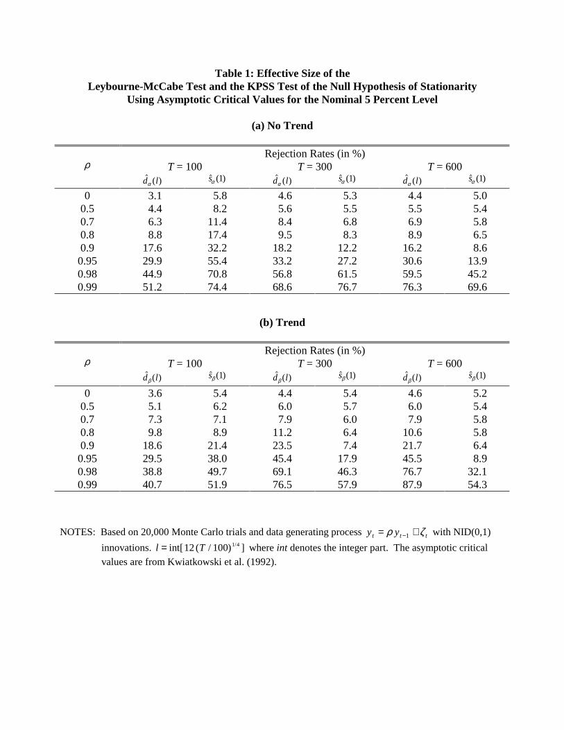
Table 1: Effective Size of theLeybourne-McCabe Test and the KPSS Test of the Null Hypothesis of Stationarity

Using Asymptotic Critical Values for the Nominal 5 Percent Level

(a) No Trend

Rejection Rates (in %)ρ T = 100 T = 300 T = 600

$ ( )d lα$ ( )sα 1 $ ( )d lα

$ ( )sα 1 $ ( )d lα$ ( )sα 1

0 3.1 5.8 4.6 5.3 4.4 5.00.5 4.4 8.2 5.6 5.5 5.5 5.40.7 6.3 11.4 8.4 6.8 6.9 5.80.8 8.8 17.4 9.5 8.3 8.9 6.50.9 17.6 32.2 18.2 12.2 16.2 8.60.95 29.9 55.4 33.2 27.2 30.6 13.90.98 44.9 70.8 56.8 61.5 59.5 45.20.99 51.2 74.4 68.6 76.7 76.3 69.6

(b) Trend

Rejection Rates (in %)ρ T = 100 T = 300 T = 600

$ ( )d lβ$ ( )sβ 1 $ ( )d lβ

$ ( )sβ 1 $ ( )d lβ$ ( )sβ 1

0 3.6 5.4 4.4 5.4 4.6 5.20.5 5.1 6.2 6.0 5.7 6.0 5.40.7 7.3 7.1 7.9 6.0 7.9 5.80.8 9.8 8.9 11.2 6.4 10.6 5.80.9 18.6 21.4 23.5 7.4 21.7 6.40.95 29.5 38.0 45.4 17.9 45.5 8.90.98 38.8 49.7 69.1 46.3 76.7 32.10.99 40.7 51.9 76.5 57.9 87.9 54.3

NOTES: Based on 20,000 Monte Carlo trials and data generating process y yt t t= +−ρ ζ1 with NID(0,1)

innovations. l T= int[ ( / ) ]12 100 1/4 where int denotes the integer part. The asymptotic criticalvalues are from Kwiatkowski et al. (1992).

Table 2: Testing for Long-Run Purchasing Power Parity in the Post-Bretton Woods Era

(a) Monthly Data

LMC KPSS DF-GLSCountry $p $ ( $)s pα $ ( )d lα

$ ( )t pφ0

Austria 1 6.026 ** 0.498 ** -0.948Belgium 7 2.045 ** 0.248 -1.581Canada 1 9.591 ** 0.670 ** -0.581Denmark 3 4.212 ** 0.299 -1.426Finland 1 0.550 ** 0.181 -1.501France 1 1.663 ** 0.223 -1.742Germany 3 3.959 ** 0.277 -1.598Greece 2 5.032 ** 0.349 * -1.850 *

Italy 3 6.320 ** 0.454 * -1.882 *

Japan 1 17.313 ** 1.324 -0.866Netherlands 3 3.238 ** 0.225 -1.570Norway 4 2.759 ** 0.197 -1.404Portugal 7 4.681 ** 0.487 ** -1.441Spain 1 1.229 ** 0.479 ** -1.170Sweden 1 4.227 ** 0.295 -2.067 *

Switzerland 1 8.906 ** 0.654 ** -0.998United Kingdom 1 4.054 ** 0.315 -1.650

Notes: All real exchange rates are constructed from IFS CD-ROM data on consumer price and end-of-period U.S.$ exchange rates. Monthly data are for 1973.1-1997.4 (292 observations). $p refers tothe Akaike Information Criterion (AIC) lag order estimate of the ARIMA(p,1,1) model. Lagorders are constrained to lie between 0 and 8. l T= int[ ( / ) ]12 100 1/4 where int denotes theinteger part. For the DF-GLS test the lag order is selected using a sequential t-test with an upperbound of p = 12. At the 5 (10) percent significance level, the asymptotic critical value for theLMC and the KPSS test is 0.463 (0.347). The finite-sample critical values for the DF-GLS testare -2.086 (-1.760). ** (*) denotes a rejection at the 5 (10) percent level.

(b) Quarterly Data

LMC KPSS DF-GLS$p $ ( $)s pα $ ( )d lα

$ ( )t pφ0

Australia 1 0.134 0.472 ** -1.311Austria 1 2.324 ** 0.265 -2.060 *

Belgium 3 0.981 ** 0.134 -2.424 **

Canada 3 2.673 ** 0.365 * -1.206Denmark 3 1.305 ** 0.166 -2.010 *

Finland 3 0.539 ** 0.100 -2.327 **

France 2 1.100 ** 0.127 -2.581 **

Germany 1 1.355 ** 0.152 -2.521 **

Greece 1 1.751 ** 0.190 -2.270 *

Ireland 2 3.697 ** 0.457 * -1.459Italy 1 2.114 ** 0.252 -2.543 **

Japan 1 6.383 ** 0.681 ** -0.734Netherlands 3 0.898 ** 0.126 -2.531 **

Norway 2 0.989 ** 0.110 -2.369 **

New Zealand 1 0.165 0.194 -2.455 **

Portugal 1 2.540 ** 0.258 -2.079 *

Spain 1 1.304 ** 0.259 -2.319 **

Sweden 3 1.203 ** 0.165 -2.741 **

Switzerland 1 0.081 0.354 * -1.857United Kingdom 1 1.536 ** 0.205 -2.367 **

Notes: All real exchange rates are constructed from IFS CD-ROM data on consumer price and end-of-period U.S.$ exchange rates. Quarterly data are for 1973.I-1997.II (98 observations). $p refers tothe Akaike Information Criterion (AIC) lag order estimate of the ARIMA(p,1,1) model. Lagorders are constrained to lie between 0 and 3 for the quarterly data. l T= int[ ( / ) ]12 100 1/4 whereint denotes the integer part. For the DF-GLS test the lag order is selected using a sequential t-testwith an upper bound of p = 8. At the 5 (10) percent significance level, the asymptotic criticalvalue for the LMC and the KPSS test is 0.463 (0.347). The finite-sample critical values for theDF-GLS test are -2.308 (-1.964). ** (*) denotes a rejection at the 5 (10) percent level.

Table 3: Power (in %) of theLMC and KPSS Tests of the Null Hypothesis of Level Stationarity

Based on Size-Adjusted Critical Values

H0: Half-Life of 3 Years H0: Half-life of 5 YearsD = 0.9439

T = 100D = 0.9809

T = 300D = 0.9659

T = 100D = 0.9885

T = 300KPSS 28.5 31.7 19.8 21.7LMC 36.7 42.5 22.2 26.8

NOTES: Based on 20,000 trials from Φ( ) ( ) ( )L L y Lt t1 1− = − θ ζ with θ = 0.25 and NID errors. Power is calculated using size-corrected critical values under the hypothesized AR(1) null.

Endnotes

1 Stationarity tests also have been modified for the purpose of testing the null of cointegration (see Harris and Inder,1994; Shin, 1994; McCabe, Leybourne, and Shin, 1997). In related work, Caner (1998) discusses applications ofstationarity tests at seasonal frequencies.2 It can be shown that this modified algorithm results in considerably lower size distortions than use of the initialvalues supplied by the GAUSS-ARIMA routine, if the test is based on asymptotic critical values. Hobijn et al.(1998) uses yet another procedure for initializing the GAUSS-ARIMA routine based on Yule-Walker estimates ofthe model under the null hypothesis. This choice of starting values has no theoretical justification under thealternative hypothesis. In this paper, we therefore rely on the procedure originally proposed by Leybourne andMcCabe.3 Lee (1996) shows that some slight improvements may be possible if we use data-based selection procedures for l,but the differences tend to be small in practice.4 After the first version of this paper was written, we became aware of a related paper by Rothman (1997) that makesa similar point. However, Rothman does not actually provide estimates of the size of the test. Moreover, his studywas limited to the KPSS test with trend, and he narrowly focused on one AR(2) DGP with a root of 0.927, T = 175and l ≤ 10.5 Sephton (1995) provides slightly more accurate critical values, but the differences are negligible for sample sizes inexcess of 100.6 We were unable to replicate the size results for the LMC test reported in Leybourne and McCabe (1994) even usingthe GAUSS code provided to us by Steve Leybourne. Even for processes with low persistence, we find much highersize distortions for the LMC test than originally reported.7 Using smaller values of l, they reject the null of stationarity for 10 of their 17 countries. This result is consistentwith evidence in Kwiatkowski et al. (1992) and Lee (1996) that small values of l tend to result in spurious rejectionsof the null hypothesis.8 Cheung and Lai (1998) analyze 3 of the 17 monthly real exchange rates used in our study using the same DF-GLStest. They are able to reject the unit root hypothesis for the U.K., France, and Germany. We obtain similar resultsfor France and Germany, but not for the U.K. The difference in the results is driven by the sample period.9 It is important to note that these size-adjusted critical values differ from the conventional finite-sample criticalvalues used for example by Culver and Papell. The latter are derived under the counterfactual assumption that thedata generating process is white noise. While they allow for the estimation of higher-order models and adjust thecritical values for the sample size, they do not adjust for the persistence of the process under the stationarity null.Thus, they are closer in spirit to the asymptotic critical values suggested by Kwiatkowski et al. (1992) than to ourcritical values.