IN THE NAME OF ALLAH, THE MOST BENEFICENT THE MOST MERCIFUL READ: In the name of your LORD Who created, created man from a clot Read: and your lord is most Bounteous Who taught by the pen Taught man that which he did not know. Taught man that which he did not know. Surah Al-Alaq (Al-Quran) Verse # (1-4) Chapter # 30

Six Phase Power Transmission System
Nov 28, 2015
A complete introduction to Six-Phase Transmission System, Components and modifications required to construct a new Six-phase line or Converting the Existing Structures of three-phase double circuit transmission lines to six-phase system. Each of the merit and demerit of Six-Phase transmission is explained by simulations and data from the actual experiments. Cost analysis is performed for New construction as well as conversion. Further research topics related to Six-phase system are also proposed
Welcome message from author
This document is posted to help you gain knowledge. Please leave a comment to let me know what you think about it! Share it to your friends and learn new things together.
Transcript

IN THE NAME OF ALLAH, THE MOST BENEFICENT THE MOST MERCIFUL
READ: In the name of your LORD Who created, created man from a clot Read: and your lord is most Bounteous
Who taught by the pen Taught man that which he did not know. Taught man that which he did not know.
Surah Al-Alaq (Al-Quran) Verse # (1-4) Chapter # 30
i
Simulation and Analysis of Six-phase Power
Transmission System
Session 2008-2012
Group Members
Safdar Rasool 2008-RCET-ELECT-02
Muhammad Kashif Nadeem 2008-RCET-ELECT-06
Muhammad Awais Rafique 2008-RCET-ELECT-16
Aamar Iqbal 2008-RCET-ELECT-22
Project Supervisor
Engr. Rehan Arif
Department of Electrical Engineering
Rachna College of Engineering and Technology, Gujranwala
(A Constituent College of University of Engineering & Technology, Lahore)
ii
Simulation and Analysis of Six-phase Power
Transmission System
Submitted to the faculty of the Electrical Engineering Department of
the University of Engineering and Technology Lahore in partial
fulfillment of the requirements for the Degree of Bachelor of Science
in
Electrical Engineering
Approval on _________________
External Examiner External Examiner
External Examiner Internal Examiner
Department of Electrical Engineering
Rachna College of Engineering and Technology, Gujranwala
(A Constituent College of University of Engineering & Technology, Lahore)

iii
Declaration
We declare that the work obtained in this report is our own, except where explicitly
stated otherwise. In addition this work has not been submitted to obtain another
degree or professional qualification.
Safdar Rasool 2008-RCET-ELECT-02 _______________________
M. Kashif Nadeem 2008-RCET-ELECT-06 _______________________
M. Awais Rafique 2008-RCET-ELECT-16 _______________________
Aamar Iqbal 2008-RCET-ELECT-22 _______________________

iv
Acknowledgment
All glory to Almighty Allah, the creator of this universe, The Gracious and
compassionate whose bounteous blessings gave us potential thoughts, talented
teachers, helping friends, loving parents, co-operative sisters and brothers and
opportunity to make this humble contribution and all praises to, respect and
‘Darood-O-Salam’ are due to His Holy Prophet(P.B.U.H) Whose blessings and
exaltations flourished our thoughts and thrived our ambition to have cherished fruit
of our modest effort in form of this write-up.
We express our most sincere gratitude, hearty sentiments and thanks to our
project advisor Engr. Rehan Arif for his excellent supervision, encouragement,
knowledge delivering. We would not have been able to complete our project
without his supervision. His sweet behavior, keen interest, personal involvement
and criticism for the betterment were all the real source of courage, inspiration and
strength during the completion of this project.

v
Dedicated to…
GREATEST REFORMER HAZRAT MUHAMMAD (PBUH) OUR
PARENTS WHO‟S PRAYERS ARE FOR US OUR TEACHERS
WHO ENCOURAGED US AT EVERY POINT OUR BROTHERS
AND SISTERS WHO’S INNOCENT SMILES ARE FUEL FOR
OUR LIFE.
vi
Table of Contents
Declaration.................................................................................................................. iii
Acknowledgment ........................................................................................................ iv
Dedicated to… ............................................................................................................. v
List of Figures .............................................................................................................. x
List of Table .............................................................................................................. xiv
List of Symbols and Acronyms ................................................................................ xv
Abstract .................................................................................................................... xvii
Chapter 1
Introduction ................................................................................................................. 1
1.1 Research Background .................................................................................... 1
1.2 Literature Assessments .................................................................................. 2
1.4 Objectives and Scope ..................................................................................... 4
1.5 Thesis structure .............................................................................................. 5
Chapter 2
Six-phase Power .......................................................................................................... 6
2.1 Introduction .................................................................................................... 6
2.2 Voltages in Six Phase System ....................................................................... 7
2.3 Phasor relationships ....................................................................................... 8
2.3.1 Phasor Relationship in Three-Phase System .......................................... 8
2.3.2 Phasor Relationship in Six-Phase System .............................................. 9
2.3.3 Phase-to-Phase Voltage ........................................................................ 10
2.3.4 Phase-to-Group Voltage ....................................................................... 11
2.3.5 Phase-to-Cross phase Voltage .............................................................. 12
2.4 Power in Six Phase System.......................................................................... 12
2.5 Advantages of Six Phase Power Transmission ........................................... 13
2.5.1 Higher Power Transfer Capability ....................................................... 13
vii
2.5.2 Increased Utilization of Right-of-Way ................................................. 14
2.5.3 Smaller Structure .................................................................................. 14
2.5.4 Lower Insulation Requirement ............................................................. 15
2.5.5 Better Stability Margin ......................................................................... 15
2.5.6 Lower Corona and Field Effects .......................................................... 15
2.5.7 Lightning Performance ......................................................................... 15
2.6 Feasibility ..................................................................................................... 16
2.7 Summary ...................................................................................................... 16
Chapter 3
Production of Six Phase Power and System components ..................................... 17
3.1 Production of Six phase ............................................................................... 18
3.1.1 Direct Six-phase Generation ................................................................ 18
3.1.2 Three-phase to Six-phase conversion .................................................. 19
3.2 Power Transformer ...................................................................................... 19
3.3 Three-Phase Transformer Connections ....................................................... 21
3.3.1 Y-Y Connection ................................................................................... 22
3.3.2 Y-∆ Connection .................................................................................... 23
3.3.3 ∆-Y Connection .................................................................................... 24
3.3.4 ∆-∆ Connection .................................................................................... 25
3.4 Six-Phase Transformer Connections............................................................ 25
3.4.1 Y-Y and Y-Inverted Y ......................................................................... 26
3.4.2 ∆-Y and ∆-Inverted Y .......................................................................... 27
3.4.3 Diametrical ........................................................................................... 28
3.4.4 Double-Delta ........................................................................................ 29
3.4.5 Double-Wye ......................................................................................... 31
3.5 Power Transmission Line ............................................................................ 31
3.5.1 Surge Impedance .................................................................................. 33
3.5.2 Surge Impedance Loading .................................................................... 33

viii
3.5.3 Line Loadability ................................................................................... 34
3.5.4 Stability Performance ........................................................................... 35
3.6 Summary ...................................................................................................... 35
Chapter 4
Modeling of six-phase Transmission System in MATLAB® ............................... 36
4.1 The Role of Simulation in Design ............................................................... 36
4.2 SimPowerSystems ....................................................................................... 36
4.3 Overview of SimPowerSystems Libraries ................................................. 38
4.4 Modeling of Three-phase double circuit line on Simulink ......................... 40
4.5 Modelling of Six-phase Transmission System ............................................ 44
4.5.1 Transformation block for wye-wye wye-inverted-wye ......................... 46
4.5.2 Delta-wye Delta Inverted wye configuration ......................................... 50
4.6 Voltage Drop Comparison ........................................................................... 55
4.7 Summary ...................................................................................................... 56
Chapter 5
Electromagnetic Field Gradients ............................................................................ 57
5.1 Magnetic Field Basics .................................................................................. 57
5.1.1 Basic Concepts: .................................................................................... 58
5.1.2 Application of Ampere’s Law to infinitely long, current carrying
conductor ............................................................................................................ 58
5.1.3 Application to Transmission Lines ...................................................... 59
5.1.4 Computer Program for calculation of Magnetic Fields ....................... 59
5.2 Magnetic field strength for Six-phase Line ................................................. 62
5.2.1 Magnetic Field of Three-Phase Double Circuit Line ........................... 62
5.2.2 Magnetic Field of Six-phase Line with same load .............................. 63
5.2.3 Magnetic Field of Six-phase Line with Increased load ....................... 64
5.2.4 Results and Conclusion ........................................................................ 65
ix
5.3 Analysis of transmission line conductor surface voltage gradients
computations ........................................................................................................... 66
5.3.2 Basic Equations .................................................................................... 67
5.3.4 Computer Program for calculation of Electric Fields .......................... 76
5.4 Corona .......................................................................................................... 78
5.4.1 Corona loss Calculations ...................................................................... 79
5.4.2 Corona Precautions for Compact Lines ................................................ 80
5.4.3 Results .................................................................................................. 82
5.5 Summary ...................................................................................................... 82
Chapter 6
System Modifications and Cost Analysis ................................................................ 83
6.1 System Modifications .................................................................................. 84
6.1.1 Six-Phase Conversion Transformers .................................................... 84
6.1.2 Six Phase Positioning ........................................................................... 84
6.1.3 Six-phase Bays ..................................................................................... 85
6.1.4 Protection .............................................................................................. 85
6.1.5 Transmission line Modifications .......................................................... 86
6.1.6 Insulation Requirements ....................................................................... 86
6.1.7 Tower Structures .................................................................................. 86
6.1.8 Right of Ways ....................................................................................... 87
6.2 Cost Analysis ............................................................................................... 87
6.3 Summary ...................................................................................................... 90
Chapter 7
Conclusions and Future Recommendations .......................................................... 91
7.1 Results and Conclusions .............................................................................. 91
7.2 Project Limitations and Future Recommendations ..................................... 93
References .................................................................................................................. 95
Appendices ............................................................................................................. 98

x
List of Figures
Chapter 2
Figure 2.1:Phasor Diagram of Six-Phase System…………………………………..7
Figure 2.2: DGC Triangle representing relationship between Vphase and Vline…..8
Figure 2.3 Phasor diagram of three phase system………………………..…………9
Figure 2.4: Potential between phase A and phase B………………………..……..11
Figure 2.5: Potential between phase A and phase C………………………………11
Figure 2.6: Potential between phase A and phase…………………………………12
Figure 2.7: Determining power density…………………………………………...14
Chapter 3
Figure 3.1: Machine Power Vs No. of Phases…………………………………….17
Figure 3.2: Six-Phase double wye Synchronous Generator……………….………18
Figure 3.3: 20 MVA three-phase transformers………………………..….……….20
Figure 3.4:Y-Y connected three-phase transformer………………………….……22
Figure 3.5: Schematic diagram of Y-Y connected three-phase transformer….…...22
Figure 3.6: Y-∆ connected three-phase transformer………………………………23
Figure 3.7: Schematic diagram of Y-∆ connected three-phase transformer……....23
Figure 3.8: ∆-Y connected three-phase transformer………………………………24
Figure 3.9: Schematic diagram of ∆-Y connected three-phase transformer………24
Figure 3.10: ∆-∆ connected three-phase transformer……………………………...25
Figure 3.11: Schematic diagram of ∆-∆ connected three-phase transformer….......25
Figure 3.12: Y-Y and Y-Inverted Y connected three-to-six-phase conversion
Transformer……………………………………………………………………….26
Figure 3.13: Schematic diagram of Y-Y and Y-Inverted Y connected three-to-six-
phase conversion transformer...................................................................................27
Figure 3.14: ∆-Y and ∆-Inverted Y connected three-to-six-phase conversion
Transformer……………………………………………………………………….27
Figure 3.15: Schematic diagram of ∆-Y and ∆-Inverted Y connected three-to-six-
phase conversion transformer……………………………………………………..28
Figure 3.16: Diametrical connected three-to-six-phase conversion
transformer………………………………………………………………………...28

xi
Figure 3.17: Schematic diagram of Diametrical connected three-to-six-phase
conversion transformer……………………………………………………………29
Figure 3.18: Double-Delta connected three-to-six-phase conversion
transformer………………………………………………………………………...29
Figure 3.19: Schematic diagram of Double-Delta connected three-to-six-phase
conversion transformer……………………………………………………………30
Figure 3.20: Double-Wye connected three-to-six-phase conversion
transformer………………………………………………………………………...30
Figure 3.21: Schematic diagram of Double-Wye connected three-to-six-phase
conversion transformer……………………………………………………………31
Figure 3.22: Lossless line terminated by its surge impedance.................................33
Figure 3.23: Surge impedance loading characteristic curve………………………34
Chapter 4
Figure 4.1: Nonlinear Simulink Blocks for SimPowerSystems Models…………..39
Figure 4.2: Simulink Library Browser…………………………………………….39
Figure 4.3: Display block for numeric display of input values……………………40
Figure 4.4: Block diagram of Three phase transformer …………………………..40
Figure 4.5: Block Diagram and Connection Diagram of Three Phase T/F……..…41
Figure 4.6: Transmission Line…………………………………………………….41
Figure 4.7: Waveform of Phase Voltages………………………………………....42
Figure 4.8: Waveform of Line Voltages………………………………………..…42
Figure 4.9: Hierarchy of Measurement blocks for Phase Voltages…………….….43
Figure 4.10: Hierarchy of Measurement blocks for Line Voltages………………..43
Figure 4.11: Complete model of Three Phase double circuit Transmission
System.......................................................................................................................44
Figure 4.12: Three-Phase RLC load………………………………………………44
Figure 4.13: Y-Y Y-Inverted Y Configuration of Transformers………………….46
Figure 4.14: Waveform of Phase voltages………………………………………...47
Figure 4.15: Waveform of Line Voltages…………………………………………47
Figure 4.16: Source Voltages………..…………………………………………….48
Figure 4.17: Voltages across Load……………………………………………...…49
Figure 4.18: Complete System for Six Phase Transmission Using Y-Y, Y-Inverted
Y Transformer configuration……………………………………………………...49
xii
Figure 4.19: Hierarchy of Delta-Wye Delta-Inverted Wye Transformation
block………………………………………………………………………………50
Figure 4.20: Waveform of Phase Voltages………………………………………..51
Figure 4.21: Waveform of Line Voltages………………………………………....51
Figure 4.22: Three-Phase RLC Load……………………………………………...52
Figure 4.23: Six Phase Transmission System using Delta-Wye Delta-Inverted Wye
Configuration of Transformer……………………………………………………..53
Figure 4.24: Diametrical Configurations……………………………………….…53
Figure 4.25: Block Diagrams………………………..……………………….........54
Figure 4.26: The connection diagram of Diametrical conversion transformer……54
Figure 4.27: Input parameter of transmission line………………………………...55
Chapter 5
Figure 5.1: The BiotSavart Law…………………………………………………...58
Figure 5.2: Magnetic field of aconductor along Z-axis carrying current I………...59
Figure 5.3: Magnetic Field of a single conductor…………………………………59
Figure 5.4: Magnetic field of a multi-conductor line……………………………...60
Figure 5.5: Relation between the lengths and Tower Geometry……………..........61
Figure 5.6: Magnetic Field Profile of Three-phase Double Circuit Transmission
Line…………………………………………………………………..……………62
Figure 5.7: Magnetic field of three-phase double circuit transmission line….........63
Figure 5.8: Magnetic field Profile of Six-phase line with same Load…………….64
Figure 5.9: Magnetic Field Profile of Six-Phase with increased load……………..65
Figure 5.10: Plot of Magnetic field of six-phase line……………………………...65
Figure 5.11: Vector addition of field due to two charges…………………….........68
Figure 5.12: Potential difference between two points a and b…………………….69
Figure 5.13:Linear path in nonunform electric field……………………………....69
Figure 5.14: Transmission line of n-conductors…………………………………..71
Figure 5.15: Electric fireld produced by source and image conductor……………73
Figure 5.16 n-conductor system………….………………………………………..75
Figure 5.17: Electric field profiles………………………………………………...77
Figure 5.18: Plot of Electric Field versus Distance for Three-Phase……………...77
Figure 5.19: Plot of Electric Field versus Distance for Six-Phase………………...78

xiii
Chapter 6
Figure 6.1: Plot of Total Line Costs for Six-phase and three-phase double circuit
lines. ……………………………………………………………………………....89

xiv
List of Tables
Chapter 2
Table 2.1 Goudy-Oakdale lightning performance flashovers per year for 2.4 km of
line ………………………………………………………………………………..16
Chapter 4
Table 4.1 Transformer configuration ………………………………..……………46
Table 4.2 Voltage Drop across the length of transmission lines for three-phase and
six-phase with 73% extra load.…………………………………………………....56
Table 4.3 Voltage drops across the length of transmission line for Six phase with
same load as three-phase…………………………………………………………..56
Chapter 5
Table 5.1: Input data for three-phase Double Circuit Transmission Line………...62
Table 5.2: Input Data for Six-phase line with same load………………….………63
Table 5.3: Input Data for Six-phase line with 73% increase in load………………64
Table 5.4: Line Configuration and Conductor Data……………………………….79
Table 5.5: Results for corona loss…………………………………………………80
Chapter 6
Table 6.1: Cost for the Equipment to be installed in Six-Phase line………………88
Table 6.2: Cost of the equipment for upgrading of three-phase double circuit line.89
xv
List of Symbols and Acronyms
α - Angular acceleration, radians/second²
δ - Angle difference between the voltages, degree
θ - Angular displacement, radians
π - 3.1416 radians or 180°
ω - Angular velocity, radians/second
a - Transformer turn ratio or 1 ∠ 120° in polar number
AC - Asynchronous current
APS - Allegheny Power Services Corporation
C - Capacitance, μF
DC - Direct current
DOE - Department of Energy
E - Excitation voltage
EHV - Extra-high voltage
f - Frequency, Hz
G - Machine rating in, MVA
GSU - Generator step-up
H - Inertia constant or Height, m
HPO - High phase order
HVDC-High-voltage DC
I - Current
L - Inductance, mH
M - Angular momentum, joule-sec/radian
MATLAB - Matrix laboratory software
MATPOWER - A MATLAB™ Power System Simulation Package
N - Number (of phases/phase conductors, turns, etc.) or Neutral
n – Speed
NTDC- National Transmission and Dispatch Company
WAPDA-Water And Power Development Authority
NYSEG - New York State Electric and Gas Corporation
NYSERDA - New York State Energy Research and Development Authority
TPDC- Three Phase double Circuit
P - Real power

xvi
Pa - Accelerating power
Pe - Electrical output of machine
Pm - Mechanical power input of machine
PSCAD/EMTDC- Power System Computer Aided Design/ Electromagnetic
Transient for Direct Current
PTI - Power Technologies Incorporated
SKVA-Three-phase apparent power, kVA
SIL - Surge Impedance Loading
Ta - Torque, Nm
UHV - Ultra-high voltages
V - Voltage
VP - Phase-to-neutral voltage
VL - Phase-to-phase voltage
VLP - Phase-to-phase voltage at primary side
VLS - Phase-to-phase voltage at secondary side
VPP - Phase-to-neutral voltage at primary side
VPS - Phase-to-neutral voltage at secondary side
W - Wide, m
x - Positive-sequence impedance, Ω
xe - System reactance, Ω
xs - Generator synchronous reactance, Ω
XL - Leakage Reactance as seen from winding 1, Ω
y - Admittance, mho
Y-Y - Wye-Wye connection of the transformer winding
Y-Δ - Wye-Delta connection of the transformer winding
Δ-Y - Delta-Wye connection of the transformer winding
Δ-Δ - Delta-Delta connection of the transformer winding
z - Impedance, Ω
Zc - Positive-sequence surge impedance of the line, Ω
xvii
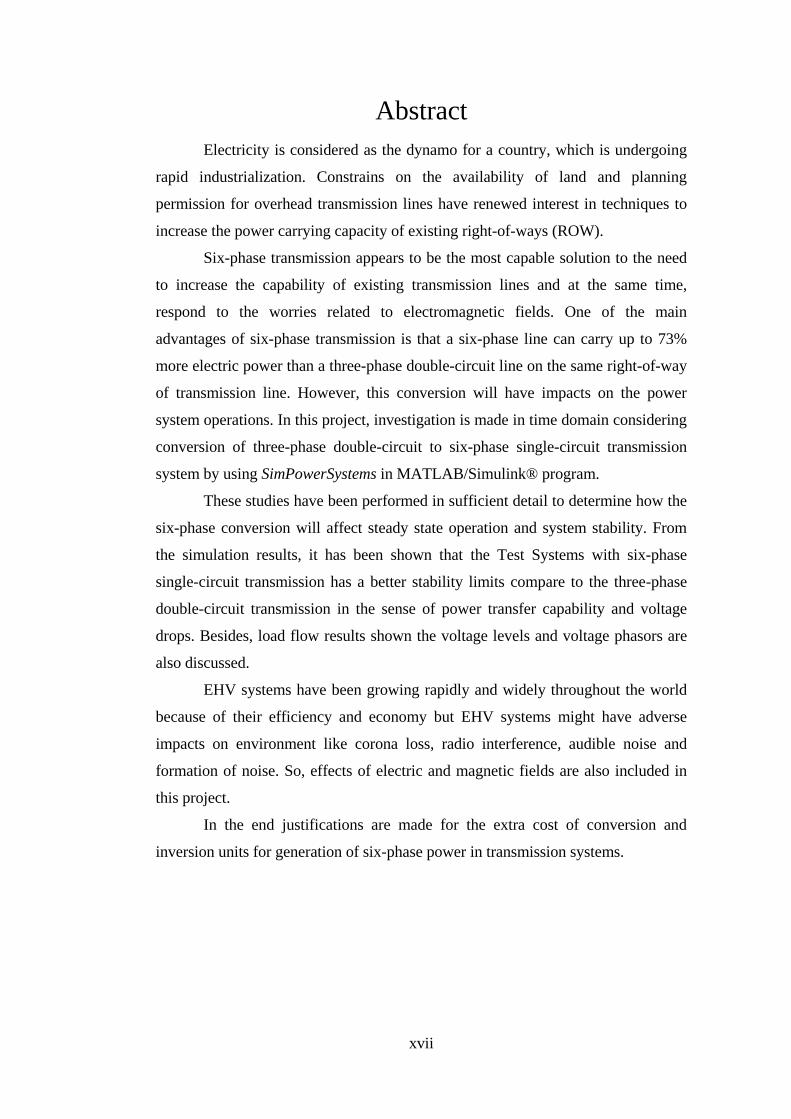
Abstract
Electricity is considered as the dynamo for a country, which is undergoing
rapid industrialization. Constrains on the availability of land and planning
permission for overhead transmission lines have renewed interest in techniques to
increase the power carrying capacity of existing right-of-ways (ROW).
Six-phase transmission appears to be the most capable solution to the need
to increase the capability of existing transmission lines and at the same time,
respond to the worries related to electromagnetic fields. One of the main
advantages of six-phase transmission is that a six-phase line can carry up to 73%
more electric power than a three-phase double-circuit line on the same right-of-way
of transmission line. However, this conversion will have impacts on the power
system operations. In this project, investigation is made in time domain considering
conversion of three-phase double-circuit to six-phase single-circuit transmission
system by using SimPowerSystems in MATLAB/Simulink® program.
These studies have been performed in sufficient detail to determine how the
six-phase conversion will affect steady state operation and system stability. From
the simulation results, it has been shown that the Test Systems with six-phase
single-circuit transmission has a better stability limits compare to the three-phase
double-circuit transmission in the sense of power transfer capability and voltage
drops. Besides, load flow results shown the voltage levels and voltage phasors are
also discussed.
EHV systems have been growing rapidly and widely throughout the world
because of their efficiency and economy but EHV systems might have adverse
impacts on environment like corona loss, radio interference, audible noise and
formation of noise. So, effects of electric and magnetic fields are also included in
this project.
In the end justifications are made for the extra cost of conversion and
inversion units for generation of six-phase power in transmission systems.
Chapter 1 Introduction
1
Chapter 1
Introduction
1.1 Research Background
Electric power has become a basic need of humanity. Its need for industrial use is
increasing day by day. That requires new generators and transmission systems to be
installed. Due to the high costs involved in the installation of new transmission
lines, engineers are looking for some alternative i.e. to enhance the power transfer
capability in the existing system. With the increase of energy demand as rapid
growth of World’s economy has caused an increased on the demand of electricity
supply and load currents of transmission lines. In the past, increase in power
transmission capability has been accomplished by increasing system voltages.
However, increasing of transmission operating voltage will produce strong electric
and magnetic fields at ground level with possible biological aspect and
environmental effects which necessitate large Right-of-Way (ROW).
In high phase order, the enhanced power system capability with the increase in 73%
load was discussed by A.S. Pandya, R.B. Kelkar [1]. The increased interest in HPO
electric power transmission over past thirty years can be traced on a CIGRE paper
published by L. D. Barthold and H.C. Barnes. Since then, the concept of HPO
transmission has become vast and it is being described in several papers and
reports.
Among the HPO techniques, 6-Φ transmission is proved to be most reliable for
increasing the capability of existing transmission lines and at the same time it deals
with electromagnetic fields as well.
One of the main advantages of 6-Φ transmission is that a 6-Φ line can carry up to
73% more electric power than a 3-Φ double-circuit line on the same transmission
Chapter 1 Introduction
2
[2]. For this reason, the current research results to have a better picture and clearer
understanding of the 6-Φ power transmission system.
In this research, study of the analysis of six phases is accomplished during normal
operating conditions for electric power system considering 3-Φ-to-6-Φ conversions
of selected transmission lines in an electric energy system.
Following analysis will be performed to know, how much 6-Φ conversion will
affect steady state operation, fault current duties, and system stability.
1. Power transmission capacity
2. Magnetic fields
3. Right of ways
4. Cost effectiveness
5. six phase transformers
These analyses will be performed on various test systems which include IEEE Test
Systems in detail using simulation program like MATLAB.
1.2 Literature Assessments
A lot of work is done on high phase order as during 1981-83 Dr P.S.Subramanyam,
S.S.Venkatetal., investigated and found different methods of 6Φ systems,
mathematical modeling of 3Φ/6Φ transformers, and calculations of inductance and
capacitance values for 6Φ lines. During 1993-94 Mr.A.K.Mishra,
Mr.Chandraserkharanetal, carried transient stability analysis of a 6Φ line using the
standard Byrd & Pichard equation which yields closed form expressions and lacks
the generality, as they are applicable to a particular simple system.
Six phase transmission is conceived as a technique to increase the power transfer
capability of existing ROW space. It was found that conversion of an existing 3-ɸ
double circuit to 6-ɸ single transmission line results in line inductance increment
and capacitance decrement. Also, it is found that voltage stability as a recent
challenging subject was analyzed. 6-ɸ single line conversion, for the length about
higher then 160KM, maximum power at the receiving end will progressively
enhance maintain the voltage stability at various power factors of load. However
the minimum line length at which power transfer capability is limited by voltage
stability concern is dramatically decreased in 6-ɸ single line compared to 3-ɸ
double circuit due to conversion transformers reactance effect. Moreover, reactive
power limit in 6 phase is increased at each point of receiving end voltage [3].
Chapter 1 Introduction
3
The incentives for increasing transmission voltages have been:
1. Reduction in ROW
2. Smaller line-voltage drops
3. Reduction in line losses
4. Lower capital and operating costs of transmission.
5. Increment in transmission distance and transmission capacity
For the purpose of transmitting power over very long distances; it may be
economical to convert the EHV AC to EHV DC, using converters we first convert
AC to DC and invert it back to AC at the other end. This is based on the fact that,
the EHV DC has lower losses in transmission line and also has no skin effect [4]. In
1954, the first modern High-Voltage DC (HVDC) transmission line was put into
operation in Sweden between Vastervik and the island of Gotland in the Baltic Sea.
HVDC lines have no reactance and are capable of transferring more power for the
same conductor size than AC lines. DC transmission is especially advantageous
when two remotely located large systems are to be connected. The DC transmission
tie line acts as an asynchronous link between the two rigid systems eliminating the
instability problem inherent in the AC links. The main disadvantage of the DC is
the production of harmonics which requires filtering, and a large amount of reactive
power compensation required at both ends of the line.
One variable which relates to that efficiency is the number of phases. The work had
focused the industry on the practical aspect of concepts that were first explained by
Fostesque [5] in 1918 and E. Clark[6] in 1943. Since this corner stone work, much
has been added to the available knowledge base on HPO transmission primarily in
the areas of feasibility considerations, analysis of system characteristics and system
protection. In the late 1970s, W. C. Guyker [7] extended the transmission concept
by describing fault analysis methodologies and symmetrical component theory.
They also assessed the feasibility of upgrading an existing 138kV line to 6-Φ to
increase the power transmission capability by 73% while reducing conductor field
gradients and improving system stability which potentially could obtain public
acceptance the nominal voltage of the line would remain unchanged.
Allegheny Power Services Corporation (APS) in cooperation with West Virginia
University began seriously investigating the details of an HPO designed in1976.
Their studies, funded partly by the National Science Foundation, showed that the
HPO transmission should be considered as a viable alternative to the conventional
Chapter 1 Introduction
4
3-Φ transmission system. They completed detailed analysis of HPO designs and
protection philosophies, but stopped short of actually demonstrating the
technologies on an operating line. Load projections for their service area were
reduced, thus eliminating the incentive to pursue increased power transfer
capabilities. The project was abandoned, however through their initiative; APS
covered the way for future research. According to new idea the feasibility of 6-Φ
transmission system is represented in terms of insulation performance, corona and
field effects, and load flow and system stability.
This study has given verification to available methods for the calculation of electric
and magnetic fields, radio noise and audio noise from the 6-Φ overhead lines. it has
been shown that the 6-Φ transmission system can provide the same power transfer
capability with lower ROW or can transfer 73% more power for the same ROW as
compared to the 3-Φ double-circuit system. Some of the advantages of using the 6-
Φ transmission system are increased transmission capability, increased utilization
of ROW, lower corona effects, lower insulation8 requirements and better voltage
regulation. Experiences with the use of the PSCAD/MATLAB software have been
positive and have enhanced the quality of research and teaching. Besides, the
simulation based approaches proved to be very effective.
1.4 Objectives and Scope
The objective of this project is to provide a solution for the limited Power
Transmission Capability of existing transmission lines and to eliminate the legal
and environmental constraints involved in the construction of new transmission
lines in the form of Electric and Magnetic field Gradients and Right of Ways
respectively. Six-phase transmission, in addition to enhanced power transmission
capability, provides low voltage gradients. Further, smaller tower structures reduce
the right of way requirements.
In this project the models of 3-Φ double-circuit transmission and 6-Φ single-circuit
transmission models by has been developed using MATALB program. Simulation
has been performed on these two transmission lines. Comparative studies for 3-Φ
double-circuit and 6-Φ single-circuit transmission lines have been implemented to
get better one out of the two for future projects.
Chapter 1 Introduction
5
1.5 Thesis structure
This thesis is primarily concerned with the understanding, modeling, and analysis
of simulation of 3-ɸ to 6-ɸ conversion of selected transmission line in electric
power system. All the work is this research is presented in chapter 4 , 5 and 6th
.
In this chapter 2 we have discussed the six-phase power system in detail. Here we
have established the definitions for system Voltages, Power and Phasor
Relationships.
In chapter 3, we establish the methods of production of Six phase power and
components used Six phase power Transmission system that include six phase
generator, six phase transformer and six phase transmission line.
In chapter 4 modeling and comparison of three-phase double circuit and six-phase
single circuit are performed in Simulink /MATLAB®. Load flow analysis and
power transfer capability comparisons are also performed.
Chapter 5 states that size of insulator required in six phase transmission towers will
be less as compared to the three-phase double circuit and size of tower will also be
compact as ground clearances and mid span clearances will be reduced. Eventually,
corona loss, radio interference, TV interference and formation of ozone due to
corona will also reduce as electric field strengths are diminished. Also it is
concluded that electric field is less for 6-ɸ than 3-ɸ.
In this chapter 6, we first discuss the modifications required in conversion of a
three-phase double circuit transmission line to a six-phase line and discussing the
savings/expenses in terms of cost in all the equipment. Later a cost analysis is
performed in which a 500kV six-phase line is compared for relative economics
with a 500 kV three-phase double circuit design.
Chapter 2 Six-phase Power
6
Chapter 2
Six-phase Power
2.1 Introduction
In recent years, rapid growth of World’s economy has caused an increase on the
demand of electricity supply. Availability of power at generation stations has
caused an increase in load currents of transmission lines to supply the growing
load. In the past, increase in power transmission capability has been accomplished
by increasing system voltages. [8] However, increasing of transmission operating
voltage will produce strong electric and magnetic field at ground level with
possible biological aspect and environmental effects which necessitate large Right-
of-Way (ROW). In consideration of the fundamental limits on power transfer
capability in a restricted ROW led to the concept of increasing the number of
phases in a transmission line system circuit also known as Multiphase system or
High Phase Order (HPO) Transmission system.
HPO is defined by number of phases of having equal magnitude of voltage but
equally spaced in time. [9] For three phase system, this means three equal
magnitude voltage vectors spaced 120o from each other. For a Six-phase this
becomes six equal magnitude voltage vectors spaced 60o between adjacent phases
and so on. Six phases have attained more importance than other HPO systems
because of its feasibility in application on existing system that is a Three Phase
Double Circuit (TPDC) Transmission Line can be converted into a six phase line
without making extraordinary modifications. As discussed earlier, the key to the
benefits of HPO transmission system lie in the Line and Phase voltage
relationships. In this chapter we have discussed the six-phase power system in
detail. Here we have established the definitions for system Voltages, Power and
Phasor Relationships.
Chapter 2 Six-phase Power
7
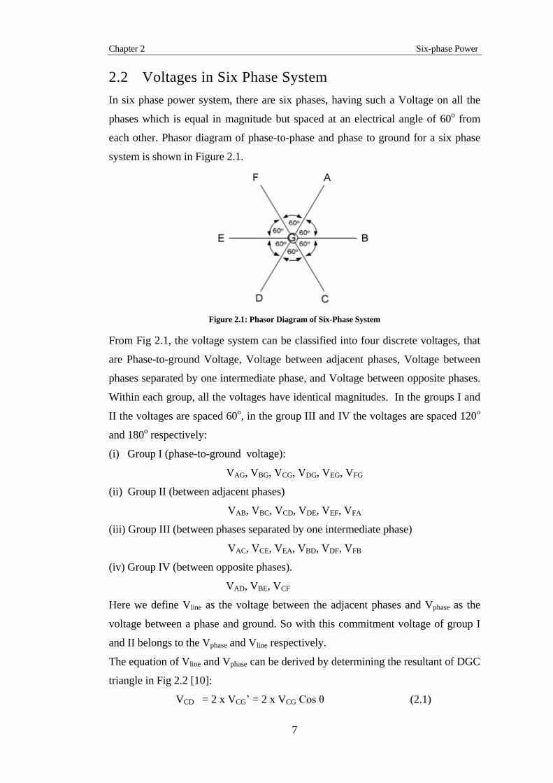
2.2 Voltages in Six Phase System
In six phase power system, there are six phases, having such a Voltage on all the
phases which is equal in magnitude but spaced at an electrical angle of 60o from
each other. Phasor diagram of phase-to-phase and phase to ground for a six phase
system is shown in Figure 2.1.
Figure 2.1: Phasor Diagram of Six-Phase System
From Fig 2.1, the voltage system can be classified into four discrete voltages, that
are Phase-to-ground Voltage, Voltage between adjacent phases, Voltage between
phases separated by one intermediate phase, and Voltage between opposite phases.
Within each group, all the voltages have identical magnitudes. In the groups I and
II the voltages are spaced 60o, in the group III and IV the voltages are spaced 120
o
and 180o respectively:
(i) Group I (phase-to-ground voltage):
VAG, VBG, VCG, VDG, VEG, VFG
(ii) Group II (between adjacent phases)
VAB, VBC, VCD, VDE, VEF, VFA
(iii) Group III (between phases separated by one intermediate phase)
VAC, VCE, VEA, VBD, VDF, VFB
(iv) Group IV (between opposite phases).
VAD, VBE, VCF
Here we define Vline as the voltage between the adjacent phases and Vphase as the
voltage between a phase and ground. So with this commitment voltage of group I
and II belongs to the Vphase and Vline respectively.
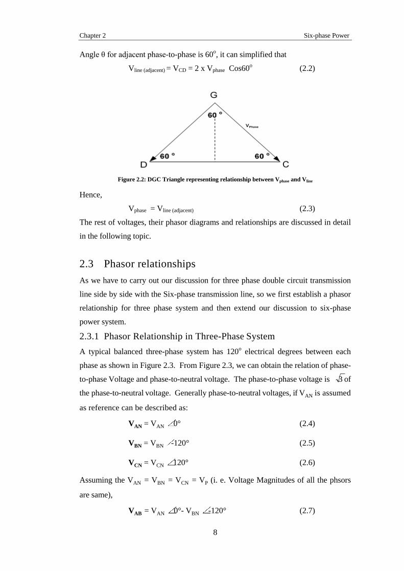
The equation of Vline and Vphase can be derived by determining the resultant of DGC
triangle in Fig 2.2 [10]:
VCD = 2 x VCG’ = 2 x VCG Cos θ (2.1)
Chapter 2 Six-phase Power
8
Angle θ for adjacent phase-to-phase is 60o, it can simplified that
Vline (adjacent) = VCD = 2 x Vphase Cos60o (2.2)
Figure 2.2: DGC Triangle representing relationship between Vphase and Vline
Hence,
Vphase = Vline (adjacent) (2.3)
The rest of voltages, their phasor diagrams and relationships are discussed in detail
in the following topic.
2.3 Phasor relationships
As we have to carry out our discussion for three phase double circuit transmission
line side by side with the Six-phase transmission line, so we first establish a phasor
relationship for three phase system and then extend our discussion to six-phase
power system.
2.3.1 Phasor Relationship in Three-Phase System
A typical balanced three-phase system has 120o electrical degrees between each
phase as shown in Figure 2.3. From Figure 2.3, we can obtain the relation of phase-
to-phase Voltage and phase-to-neutral voltage. The phase-to-phase voltage is 3 of
the phase-to-neutral voltage. Generally phase-to-neutral voltages, if VAN is assumed
as reference can be described as:
VAN = VAN 0° (2.4)
VBN = VBN -120° (2.5)
VCN = VCN 120° (2.6)
Assuming the VAN = VBN = VCN = VP (i. e. Voltage Magnitudes of all the phsors
are same),
VAB = VAN 0°- VBN -120° (2.7)
Chapter 2 Six-phase Power
9
= VP (1 0°- 1 -120°)
= VP (1+j0 - (-0.5 - j0.866))
= VP (1.5 + j0.866)
= 3 VP 30° (2.8)
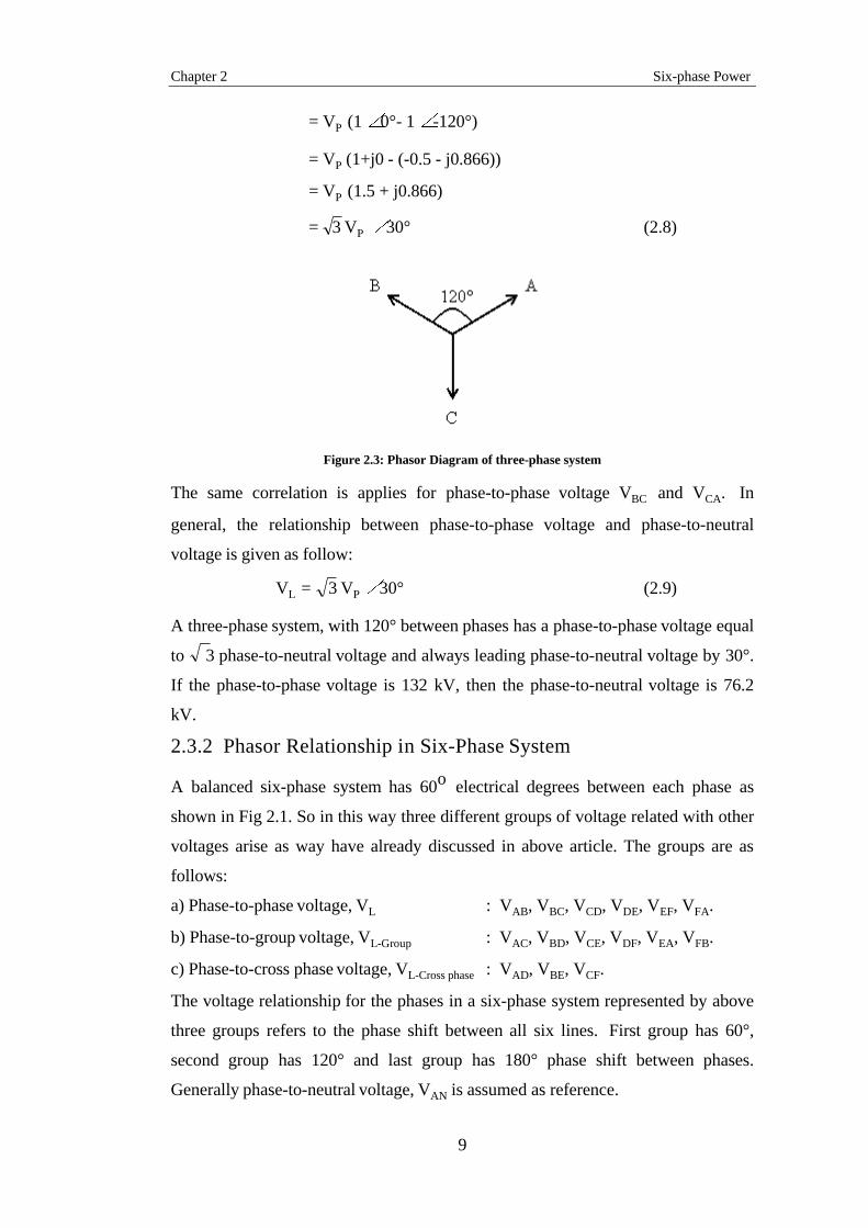
Figure 2.3: Phasor Diagram of three-phase system
The same correlation is applies for phase-to-phase voltage VBC and VCA. In
general, the relationship between phase-to-phase voltage and phase-to-neutral
voltage is given as follow:
VL = 3 VP 30° (2.9)
A three-phase system, with 120° between phases has a phase-to-phase voltage equal
to 3 phase-to-neutral voltage and always leading phase-to-neutral voltage by 30°.
If the phase-to-phase voltage is 132 kV, then the phase-to-neutral voltage is 76.2
kV.
2.3.2 Phasor Relationship in Six-Phase System
A balanced six-phase system has 60o
electrical degrees between each phase as
shown in Fig 2.1. So in this way three different groups of voltage related with other
voltages arise as way have already discussed in above article. The groups are as
follows:
a) Phase-to-phase voltage, VL : VAB, VBC, VCD, VDE, VEF, VFA.
b) Phase-to-group voltage, VL-Group : VAC, VBD, VCE, VDF, VEA, VFB.
c) Phase-to-cross phase voltage, VL-Cross phase : VAD, VBE, VCF.
The voltage relationship for the phases in a six-phase system represented by above
three groups refers to the phase shift between all six lines. First group has 60°,
second group has 120° and last group has 180° phase shift between phases.
Generally phase-to-neutral voltage, VAN is assumed as reference.
Chapter 2 Six-phase Power
10
VAN = VAN 0°
VBN = VBN -60°
VCN = VCN -120°
VDN = VDN -180°
VEN = VEN -240°
VFN = VFN -300°
2.3.3 Phase-to-Phase Voltage
We have already obtained a relationship between phase-to-phase voltage and phase-
to-neutral voltage for a six-phase system mathematically. Now we obtain the same
using an alternate method.
Phase-to-phase voltage is a potential between adjacent phases where their phase
difference is 60°. Fig 2.4 shows the potential between phase A and phase B.
Assuming the VAN = VBN = VCN = VDN = VEN = VFN =VP,
VAB = VAN 0°- VBN -60°
= VP (1 0°- 1 -60°)
= VP (1+j0 - (0.5 - j0.866))
= VP (0.5 + j0.866)
= VP 60° (2.10)
The same correlation is applied for phase-to-phase voltages VAB, VBC, VCD, VDE,
VEF and VFA. For a six-phase system, the magnitude of phase-to-phase voltage is
equal to the magnitude of the phase-to-neutral voltage and phase-to-phase voltage
always leading the phase-to-neutral voltage by 60°. In general, the relationship
between phase-to-phase voltage and phase-to-neutral voltage is given as follow:
VL = V
P 60° (2.11)

Chapter 2 Six-phase Power
11
Figure 2.4: Potential between phase A and phase B
2.3.4 Phase-to-Group Voltage
Phase-to-group voltage is a potential between phases where the phase difference is
120°. Fig 2.5 shows the potential between phase A and phase C.
VAC = VAN 0°- VCN ∠ -120°
= VP (1 0°- 1 -120°)
= VP (1+j0 - (-0.5 - j0.866))
= VP (1.5 + j0.866)
= 3 VP 30° (2.12)
The same correlation is applies for phase-to-phase voltages VAC, VBD, VCE, VDF,
VEA and VFB. The magnitude of phase-to-group voltage is 3 times the magnitude
of the phase-to-neutral voltage and phase-to-phase voltage always leading the
phase-to- neutral voltage by 30°. In general, the relationship between phase-to-
group voltage and phase-to-neutral voltage is given as follow:
VL-Group = 3 V
P 30° (2.13)
Figure 2.5: Potential between phase A and phase C

Chapter 2 Six-phase Power
12
2.3.5 Phase-to-Cross phase Voltage
Phase-to-crossphase voltage is a potential between phases where the phase
difference is 180°. Fig 2.6 shows the potential between phase A and phase D.
VAD = VAN 0°- VDN -180°
= VP (1 0°- 1 -180°)
= VP (1+j0 - (-1.0 + j0))
= VP (2)
= 2VP 0° (2.14)
The same correlation is applies for phase-to-phase voltages VAD, VBE and VCF. The
magnitude of phase-to-cross phase voltage is two times the magnitude of the phase-
to-neutral voltage. In general, the relationship between phase-to-crossphase voltage
and phase-to-neutral voltage is given as follow:
VL-Crossphase = 2V
P 0° (2.15)
Figure 2.6: Potential between phase A and phase
2.4 Power in Six Phase System
Assuming unity power factor power in a three phase double circuit transmission
line can be calculated using following formula.
Pthree-phase-double-circuit = 2 (3 Vphase-to-neutral Iline) (2.16)
= 6 Vphase to neutral (3 phase) Iline
Whereas power in Six-phase line can be calculated as:
PSix-phase = 6 Vphase to neutral (6 phase) Iline (2.17)
If a three-phase double circuit line is upgraded to a six phase line, keeping Vphase to
neutral (3 phase) equal to Vphase to neutral (6 phase), there is no increase in power, but the
Chapter 2 Six-phase Power
13
increase is in power density. That is, the Right of Way (ROW) requirement is
reduced due to the reduction in electric and magnetic field gradients. This also
results in smaller supporting structures, less conductor spacing and low insulation
requirement.
On the other hand, if a Vphase to neutral (6 phase) is increased to Vline-to-line (3 phase), there is
73% increase in power, consuming the same ROW and having same electric and
magnetic field strengths. Increase in power can be evaluated as:
Since,
Vphase to neutral (6 phase) = Vline to line = 3 Vphase to neutral (3 phase)
So, from equation 2.16 can be written for six phase power as:
PSix-phase = 6 Vphase to neutral (6 phase) Iline
= 6( 3 Vphase to neutral (3 phase) ) Iline
= 3 (6Vphase to neutral (3 phase) Iline )
= 3 Pthree-phase-double-circuit
= 1.73 Pthree-phase-double-circuit
Because Vphase to neutral (6 phase) is 3 (or 1.73) times higher than Vphase to neautral (3 phase),
hence, the main advantage of a six-phase transmission line is that it can carry it can
carry up to 73% more electric power transfer capability compare to a three-
phase system at the same operating voltage.
2.5 Advantages of Six Phase Power Transmission
With the growing concern over the environmental effects of power system, six-
phase transmission offers several advantages over conventional three-phase double-
circuit networks. The following subtitles show the advantages of six-phase
transmission line. These benefits are among the reasons why power system
engineers are consistently pursues knowledge on the power system technology.
2.5.1 Higher Power Transfer Capability
Power transmission capability is directly proportional to phase-to-phase voltage. As
seen by the phasor relationship, for the same phase-to-phase voltage as in the three-
phase system, a six-phase system has a 73% increase in phase-to-neutral voltage.
Therefore, it can be observed that, when a three-phase double-circuit line is
converted to six-phase line, the power capability is increased by 73%. This
Chapter 2 Six-phase Power
14
phenomenon has already been proved in article 2.4 that power in six-phase is 1.73
times that of three-phase double circuit transmission line.
2.5.2 Increased Utilization of Right-of-Way
Six-phase transmission increases power density. Power density refers to the amount
of power that can be transmitted down a given window of ROW assuming there are
environmental and technical constraints that limit size of ROW. Thus, these lines
can transfer more power over a given ROW than equivalently loaded three-phase
lines [12].
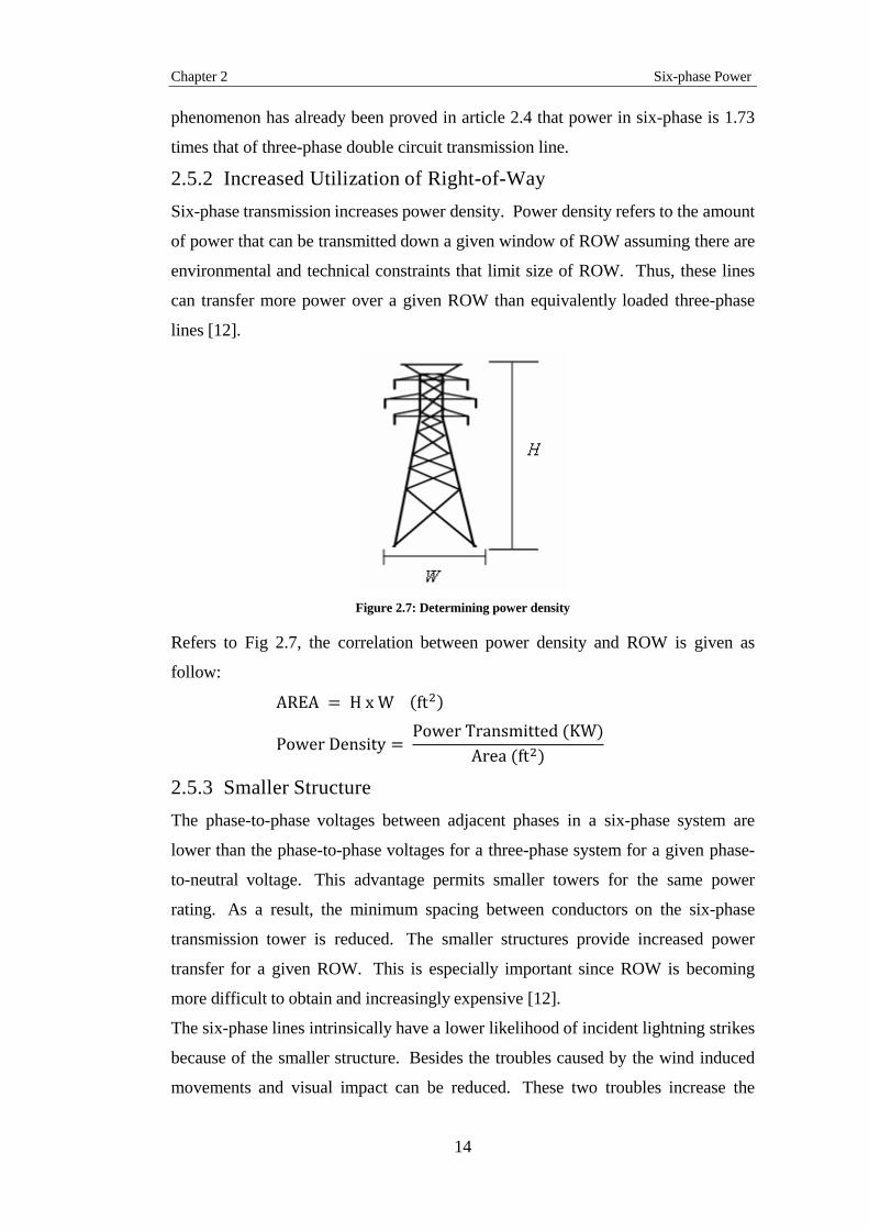
Figure 2.7: Determining power density
Refers to Fig 2.7, the correlation between power density and ROW is given as
follow:
( )
( )
( )
2.5.3 Smaller Structure
The phase-to-phase voltages between adjacent phases in a six-phase system are
lower than the phase-to-phase voltages for a three-phase system for a given phase-
to-neutral voltage. This advantage permits smaller towers for the same power
rating. As a result, the minimum spacing between conductors on the six-phase
transmission tower is reduced. The smaller structures provide increased power
transfer for a given ROW. This is especially important since ROW is becoming
more difficult to obtain and increasingly expensive [12].
The six-phase lines intrinsically have a lower likelihood of incident lightning strikes
because of the smaller structure. Besides the troubles caused by the wind induced
movements and visual impact can be reduced. These two troubles increase the
Chapter 2 Six-phase Power
15
cause of maintenance for the structures of the transmission line and which,
sometimes may cause the danger of life [12].
2.5.4 Lower Insulation Requirement
For a six-phase system, the insulation required to support one phase from an
adjacent phase is equal to that required to support a phase from the zero potential
point. Thus, utilities can save on various insulating materials for various
components of transmission system [13].
2.5.5 Better Stability Margin
A six-phase line can be operated at a smaller power angle than a three-phase line.
This means that the six-phase line offers better stability margin than its three- phase
counterpart [11].
2.5.6 Lower Corona and Field Effects
Conversion from three-phase double-circuit to six-phase single-circuit has the effect
of reducing electric field at the conductor surface for the same phase-to-neutral
voltage. Conductor gradients decrease as the number of phases increases for a
given conductor size and tower configuration. Thus, radio and audio noise can be
reduced which in turn leads to lesser television and radio interference. The
reduction in electric field can be utilized in either of two ways:
a) Increase the phase-to-neutral voltage until the conductor surface electric field is
a maximum for corona thus increasing the power handling capacity of the line.
b) Maintain the same phase-to-neutral voltage and decrease the conductor spacing
until the conductor surface electric field is a maximum for corona, thus making
the line more compact.
2.5.7 Lightning Performance
When the line is converted to six-phase operation, there is an increase in the
shielding failure rate and a reduction in the back flash rate, resulting in a net
reduction in the trip out rate. However, the total flashovers are so close before and
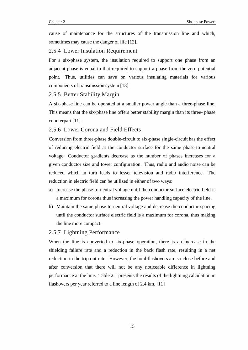
after conversion that there will not be any noticeable difference in lightning
performance at the line. Table 2.1 presents the results of the lightning calculation in
flashovers per year referred to a line length of 2.4 km. [11]
Chapter 2 Six-phase Power
16
Table 2.1: Goudey-Oakdale lightning performance flashovers per year for 2.4 km of line [11]
2.6 Feasibility
The aim of improving efficiency of transmission network is indeed the driving
factor for electrical utility engineers to consider the six-phase transmission. Six-
phase transmission system offers the opportunity to meet the increasing demands
for power yet at the same time meet the environmental and regulatory constraints.
However, the economy factors have to be considered. Terminal expenses can be
quite high for six-phase lines. A six-phase line would require conversion
transformers that would cause the terminals to be more costly. The high cost of
terminals is offset by reduced tower and lower foundation costs, ROW cost and
losses.
2.7 Summary
This chapter describes the basics about six phase power and also gives an insight to
its advantages and benefits. Basic idea in six phase power transmission is
introduced. Complexities in voltage in six-phase are discussed. Moreover, the
phasors relationship for both three-phase and six-phase system is discussed in
detail. For a three-phase system, phase-to-phase voltage is equal to 3 phase-to-
neutral voltage. The phase-to-phase voltages always lead the phase-to-neutral
voltage by 30°. In a six-phase system, the phasors relationship can be divided into
three categories. They are categorized depends to the phase difference between
phases which is 60°, 120° and 180°. These categories are phase-to-phase voltages,
phase-to-group voltages and phase-to-cross phase voltages. As proves that
discussed in this chapter, six-phase have a great deal of advantages over three-
phase transmission system.
Configuration Shielding Failures Back flashes Total
115 kV three-phase 0.029 0.126 0.155
93 kV six-phase 0.049 0.077 0.127

Chapter 3 Production of Six Phase Power and System Components
17
Chapter 3
Production of Six Phase Power
and System components
Bulk power transmission systems in world are majorly utilizing AC transmission to
transfer power do so via three phases. Historically this came about because three-
phase AC is the most efficient way to generate power. Generating power with
electrical angles less than 120 degrees between phases does not result in a
corresponding increase in power output (see Fig 3.1). With AC power being
generated at 3 phase it was logical to transfer that power in a similar manner and
hence the three phase power transmission system was born. . [12]
Figure 3.1: Machine Power Vs No. of Phases
The concept of using transmission systems that carry power with more than three
phases is a relatively new idea. As stated earlier, it was first proposed as part of an
international electrical committee study in 1973. The idea was relatively straight
Chapter 3 Production of Six Phase Power and System Components
18
forward. Instead of transmitting power with the same number of phases as it was
generated, Six-phase transmission would alter the power generated into 6 phases.
This process would allow for some unique benefits that are described in previous
chapter.
Before moving on the modeling and detailed analysis, the devices/components to
be used in Six Phase power system should be analyzed. In this chapter, the methods
of production of Six phase power and components used Six phase power
Transmission system are analyzed that include six phase generator, six phase
transformer and six phase transmission line.
3.1 Production of Six phase
Six phase power can be produced in multiple ways. Two major methods for the
production of Six phase are:
i) Direct Six-phase Generation
ii) 3-phase to 6-phase conversion
Detail of each method is given below.
3.1.1 Direct Six-phase Generation
As discussed earlier, the generation in three-phase is the most efficient way to
generate electric power [12]. However, six-phase power can be directly generated
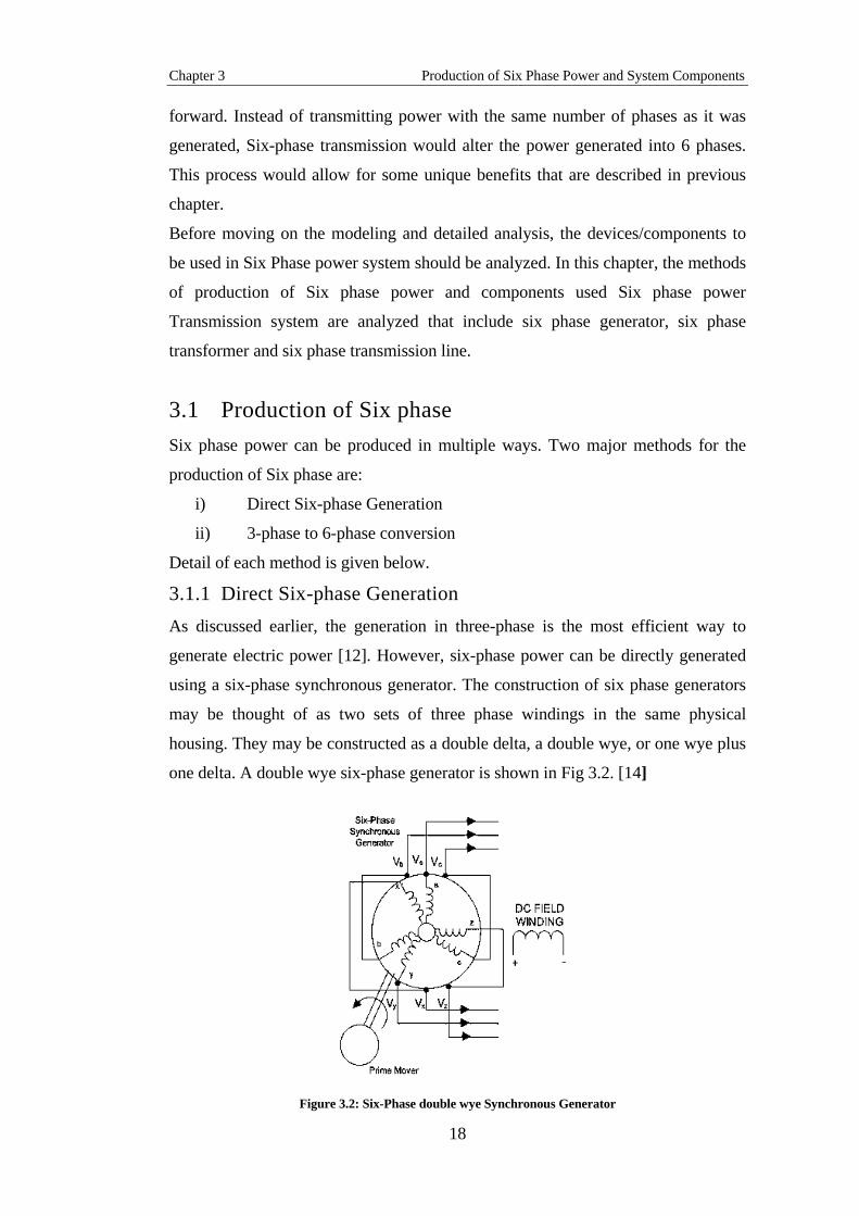
using a six-phase synchronous generator. The construction of six phase generators
may be thought of as two sets of three phase windings in the same physical
housing. They may be constructed as a double delta, a double wye, or one wye plus
one delta. A double wye six-phase generator is shown in Fig 3.2. [14]
Figure 3.2: Six-Phase double wye Synchronous Generator
Chapter 3 Production of Six Phase Power and System Components
19
However, six-phase generator does not have its practical applications for power
generation in bulk due to its higher complexity and less efficiency than three-phase
generation machines. It finds its application in speed control of drives and
renewable energy generation.
3.1.2 Three-phase to Six-phase conversion
The other and most feasible method for the production of six phase is by using
three phase to six phase conversion transformer bank. A six-phase to three-phase or
three-phase to six-phase conversion transformer can be constructed by two
techniques.
First, six identical single phase two winding transformers may be connected to form
three to six-phase transformer bank. Secondly, three identical single phase three
winding transformers may be connected together to form three to six-phase
transformer bank. Voltage and current magnitude depends on the windings
connections. The details about transformer connections and their characteristics are
discussed in the next articles.
Following article deals with the Power Transformer to be used in Six-phase
Transmission. It establishes the definition of transformer, discussed three-phase
transformer and then leads to the six-phase transformer and its connection.
3.2 Power Transformer
A transformer is defined as a static electrical device, involving no continuously
moving parts, used in electric power systems to transfer power between circuits
through the use of electromagnetic induction. The term power transformer is used
to refer to those transformers used between the generator and the distribution
circuits and are usually rated at 500 kVA and above. The power transformer is a
major power system component that permits economic power transmission with
high efficiency and low series-voltage drops. Since electric power is proportional to
the product of voltage and current, low current levels (and therefore low I²R losses
and low IZ voltage drops) can be maintained for given power levels at the expense
of high voltages. Power systems typically consist of a large number of generation
locations, distribution points, and interconnections within the system or with nearby
systems, such as a neighboring utility. Power transformers are selected based on
the application, with the emphasis towards custom design being more apparent the
larger the unit. Power transformers are available for step-up operation, primarily
Chapter 3 Production of Six Phase Power and System Components
20
used at the generator and referred to as step-up transformers (SUT), and for step-
down operation, mainly used to feed distribution circuits. Power transformers are
available as a single-phase or three-phase apparatus. The construction of a
transformer depends upon the application, with transformers intended for indoor use
primarily dry-type but also as liquid immersed transformers are used and for outdoor
use usually liquid immersed transformers are used. The example of outdoor liquid-
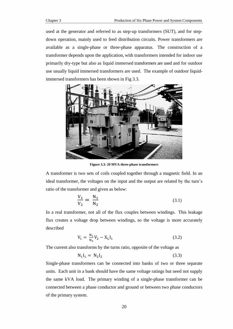
immersed transformers has been shown in Fig 3.3.
Figure 3.3: 20 MVA three-phase transformers
A transformer is two sets of coils coupled together through a magnetic field. In an
ideal transformer, the voltages on the input and the output are related by the turn’s
ratio of the transformer and given as below:
(3.1)
In a real transformer, not all of the flux couples between windings. This leakage
flux creates a voltage drop between windings, so the voltage is more accurately
described
(3.2)
The current also transforms by the turns ratio, opposite of the voltage as
(3.3)
Single-phase transformers can be connected into banks of two or three separate
units. Each unit in a bank should have the same voltage ratings but need not supply
the same kVA load. The primary winding of a single-phase transformer can be
connected between a phase conductor and ground or between two phase conductors
of the primary system.
Chapter 3 Production of Six Phase Power and System Components
21
3.3 Three-Phase Transformer Connections
Three-phase transformers have one coaxial coil for each phase encircling a vertical
leg of the core structure. Stacked cores have three or possibly four vertical legs,
while wound cores have a total of four loops creating five legs or vertical paths:
three down through the center of the three coils and one on the end of each outside
coil. The use of three versus four or five legs in the core structure has a bearing on
which electrical connections and loads can be used by a particular transformer. The
advantage of three-phase electrical systems in general is the economy gained by
having the phases share common conductors and other components. This is
especially true of three-phase transformers using common core structures. Three-
phase transmission line terminal transformer services are normally constructed from
three single- phase units. Three-phase transformers for underground service (either
pad mounted, direct buried, or in a vault or building or manhole) are normally single
units, usually on a three- or five-legged core. The kVA rating for a three-phase
bank is the total of all three phases. The full-load current in amps in each phase of a
three-phase unit or bank is:
√ (3.4)
There are two ways that can be used to construct a three-phase transformer. First,
three identical single-phase two-winding transformers may be connected to form
three-phase bank. Secondly, a three-phase transformer can be constructed by
winding three single-phase transformers on a single core. Voltage and current
magnitude depends on the windings connection used at the primary and the
secondary sides of that three-phase transformer. The primary or secondary sides of
the three-phase transformer may be connected by using either Wye (Y) or Delta (∆)
connections. There are four common combinations used in three-phase transformer
which is, Y-Y, Y-∆, ∆-Y, ∆-∆.
i. Wye-Wye, (Y-Y)
ii. Wye-Delta (Y-∆)
iii. Delta-Wye (∆-Y)
iv. Delta-Delta (∆-∆)
3.3.1 Y-Y Connection
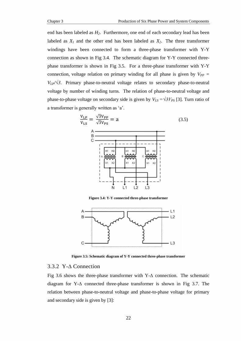
The three transformer windings in Fig 3.4 have been labeled as A, B and C
respectively. One end of each primary lead has been labeled as H1 and the other
Chapter 3 Production of Six Phase Power and System Components
22
end has been labeled as H2. Furthermore, one end of each secondary lead has been
labeled as X1 and the other end has been labeled as X2. The three transformer
windings have been connected to form a three-phase transformer with Y-Y
connection as shown in Fig 3.4. The schematic diagram for Y-Y connected three-
phase transformer is shown in Fig 3.5. For a three-phase transformer with Y-Y
connection, voltage relation on primary winding for all phase is given by VPP =
VLP/√3. Primary phase-to-neutral voltage relates to secondary phase-to-neutral
voltage by number of winding turns. The relation of phase-to-neutral voltage and
phase-to-phase voltage on secondary side is given by VLS =√3VPS [3]. Turn ratio of
a transformer is generally written as ‘a’.
√
√ (3.5)
Figure 3.4: Y-Y connected three-phase transformer
Figure 3.5: Schematic diagram of Y-Y connected three-phase transformer
3.3.2 Y-∆ Connection
Fig 3.6 shows the three-phase transformer with Y-∆ connection. The schematic
diagram for Y-∆ connected three-phase transformer is shown in Fig 3.7. The
relation between phase-to-neutral voltage and phase-to-phase voltage for primary
and secondary side is given by [3]:
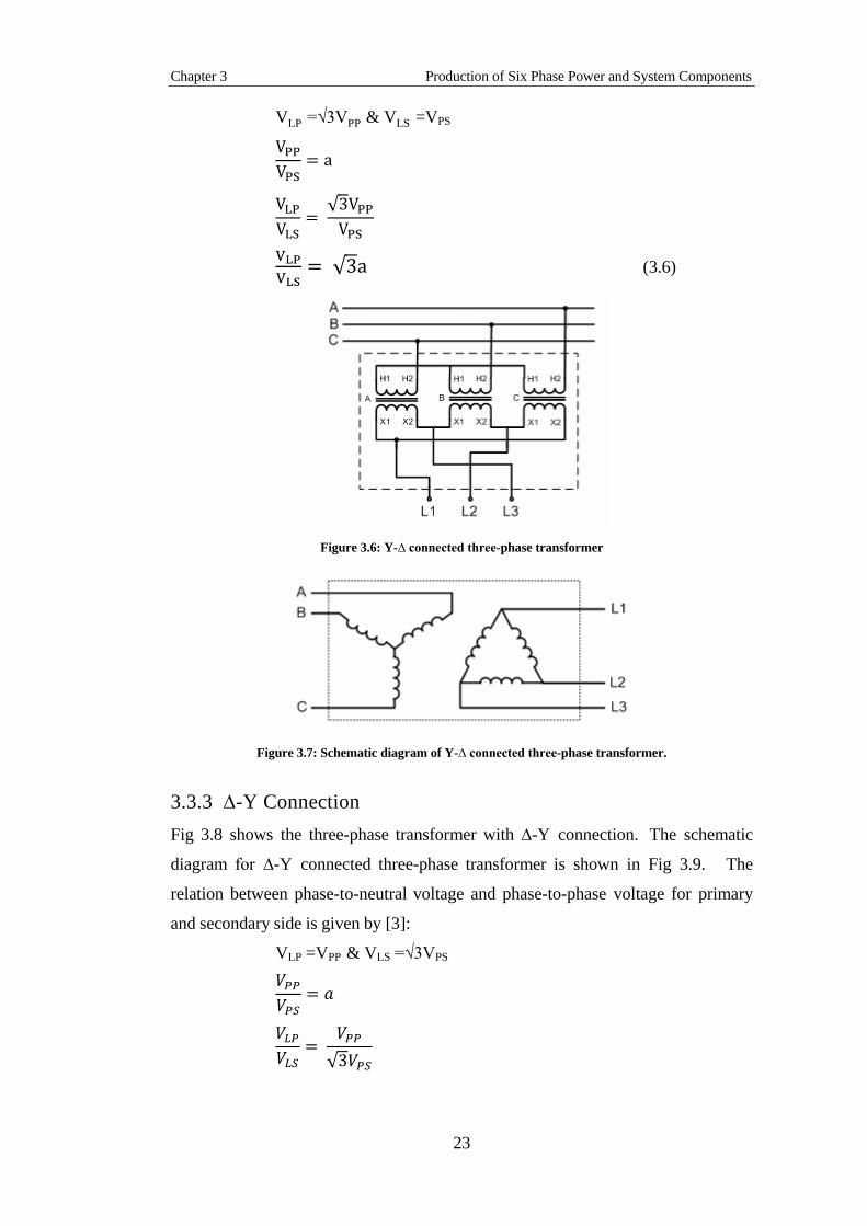
Chapter 3 Production of Six Phase Power and System Components
23
VLP =√3VPP & VLS =VPS
√
√ (3.6)
Figure 3.6: Y-∆ connected three-phase transformer
Figure 3.7: Schematic diagram of Y-∆ connected three-phase transformer.
3.3.3 ∆-Y Connection
Fig 3.8 shows the three-phase transformer with ∆-Y connection. The schematic
diagram for ∆-Y connected three-phase transformer is shown in Fig 3.9. The
relation between phase-to-neutral voltage and phase-to-phase voltage for primary
and secondary side is given by [3]:
VLP =VPP & VLS =√3VPS
√
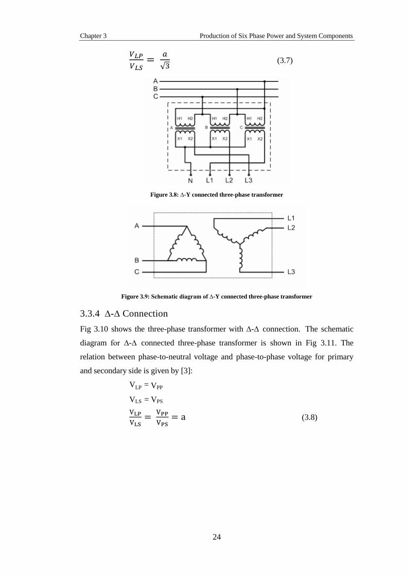
Chapter 3 Production of Six Phase Power and System Components
24
√ (3.7)
Figure 3.8: ∆-Y connected three-phase transformer
Figure 3.9: Schematic diagram of ∆-Y connected three-phase transformer
3.3.4 ∆-∆ Connection
Fig 3.10 shows the three-phase transformer with ∆-∆ connection. The schematic
diagram for ∆-∆ connected three-phase transformer is shown in Fig 3.11. The
relation between phase-to-neutral voltage and phase-to-phase voltage for primary
and secondary side is given by [3]:
VLP = VPP
VLS = VPS
(3.8)
Chapter 3 Production of Six Phase Power and System Components
25
Figure 3.10: ∆-∆ connected three-phase transformer
Figure 3.11: Schematic diagram of ∆-∆ connected three-phase transformer.
3.4 Six-Phase Transformer Connections
As discussed earlier, there are two types of single-phase transformers that can be
used to build a three-to-six-phase conversion transformer. First, six identical single-
phase two-winding transformers may be connected to form three-to-six-phase bank.
Secondly, three identical single-phase three-winding transformers may be connected
together to form three-to-six-phase bank. Voltage and current magnitude depends
on the windings connection used on the primary and the secondary sides of the
three-to-six-phase conversion transformer. The primary or secondary side of the
three-to-six-phase conversion transformer may be connected by using any
combinations of either Wye (Y) or Delta (∆) connections. There are five common
connections and combinations that can be used to form a three-to-six-phase
conversion transformer which is Y-Y and Y-Inverted Y, ∆-Y & ∆-Inverted Y,
Diametrical, Double-Delta and Double- Wye.
3.4.1 Y-Y and Y-Inverted Y
The six transformer windings in Fig 3.12 have been labeled as A, B, C, D, E and F
respectively. One end of each primary lead has been labeled as H1 and the other
end has been labeled as H2. Furthermore, one end of each secondary lead has been
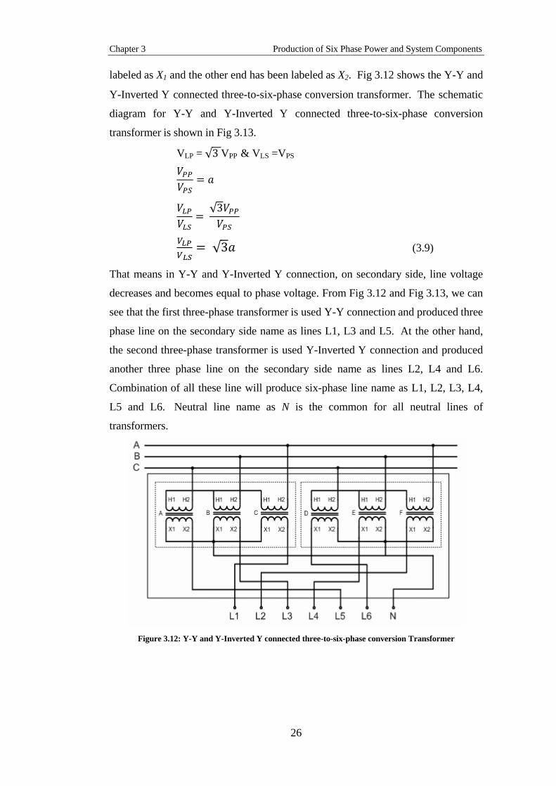
Chapter 3 Production of Six Phase Power and System Components
26
labeled as X1 and the other end has been labeled as X2. Fig 3.12 shows the Y-Y and
Y-Inverted Y connected three-to-six-phase conversion transformer. The schematic
diagram for Y-Y and Y-Inverted Y connected three-to-six-phase conversion
transformer is shown in Fig 3.13.
VLP = √ VPP & VLS =VPS
√
√ (3.9)
That means in Y-Y and Y-Inverted Y connection, on secondary side, line voltage
decreases and becomes equal to phase voltage. From Fig 3.12 and Fig 3.13, we can
see that the first three-phase transformer is used Y-Y connection and produced three
phase line on the secondary side name as lines L1, L3 and L5. At the other hand,
the second three-phase transformer is used Y-Inverted Y connection and produced
another three phase line on the secondary side name as lines L2, L4 and L6.
Combination of all these line will produce six-phase line name as L1, L2, L3, L4,
L5 and L6. Neutral line name as N is the common for all neutral lines of
transformers.
Figure 3.12: Y-Y and Y-Inverted Y connected three-to-six-phase conversion Transformer
Chapter 3 Production of Six Phase Power and System Components
27
Figure 3.13: Schematic diagram of Y-Y and Y-Inverted Y connected three-to-six- phase conversion
transformer.
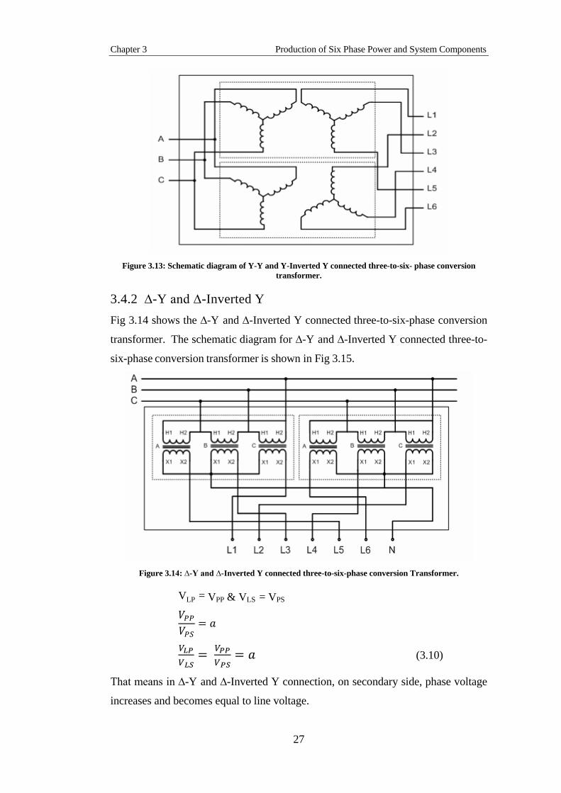
3.4.2 ∆-Y and ∆-Inverted Y
Fig 3.14 shows the ∆-Y and ∆-Inverted Y connected three-to-six-phase conversion
transformer. The schematic diagram for ∆-Y and ∆-Inverted Y connected three-to-
six-phase conversion transformer is shown in Fig 3.15.
Figure 3.14: ∆-Y and ∆-Inverted Y connected three-to-six-phase conversion Transformer.
VLP = VPP & VLS = VPS
(3.10)
That means in ∆-Y and ∆-Inverted Y connection, on secondary side, phase voltage
increases and becomes equal to line voltage.

Chapter 3 Production of Six Phase Power and System Components
28
Figure 3.15: Schematic diagram of ∆-Y and ∆-Inverted Y connected three-to-six- phase conversion
transformer.
3.4.3 Diametrical
Fig 3.16 shows the Diametrical connected three-to-six-phase conversion
transformer. The schematic diagram for Diametrical connected three-to-six-phase
conversion transformer is shown in Fig 3.17.
Figure 3.16: Diametrical connected three-to-six-phase conversion transformer
VLP = VPP & VLS = VPS
(3.11)

Chapter 3 Production of Six Phase Power and System Components
29
That means in diametrical connection, on secondary side, phase voltage increases
and becomes equal to line voltage.
Figure 3.17: Schematic diagram of Diametrical connected three-to-six-phase conversion transformer.
3.4.4 Double-Delta
Fig 3.18 shows the Double-Delta connected three-to-six-phase conversion
transformer. The schematic diagram for Double-Delta connected three-to-six-phase
conversion transformer is shown in Fig 3.19.
Figure 3.18: Double-Delta connected three-to-six-phase conversion transformer
VLP = √ VPP & VLS =VPS
√
Chapter 3 Production of Six Phase Power and System Components
30
√ (3.12)
That means in Double Delta connection, on secondary side, line voltage decreases
and becomes equal to phase voltage.
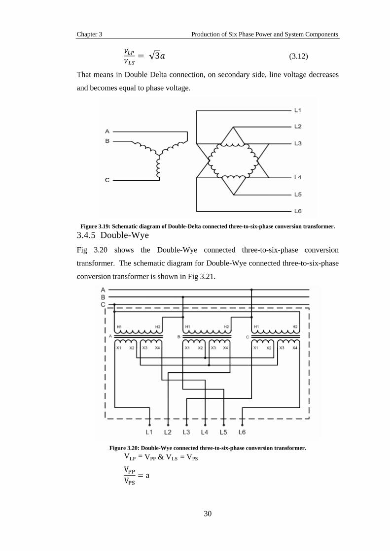
Figure 3.19: Schematic diagram of Double-Delta connected three-to-six-phase conversion transformer.
3.4.5 Double-Wye
Fig 3.20 shows the Double-Wye connected three-to-six-phase conversion
transformer. The schematic diagram for Double-Wye connected three-to-six-phase
conversion transformer is shown in Fig 3.21.
Figure 3.20: Double-Wye connected three-to-six-phase conversion transformer.
VLP = VPP & VLS = VPS
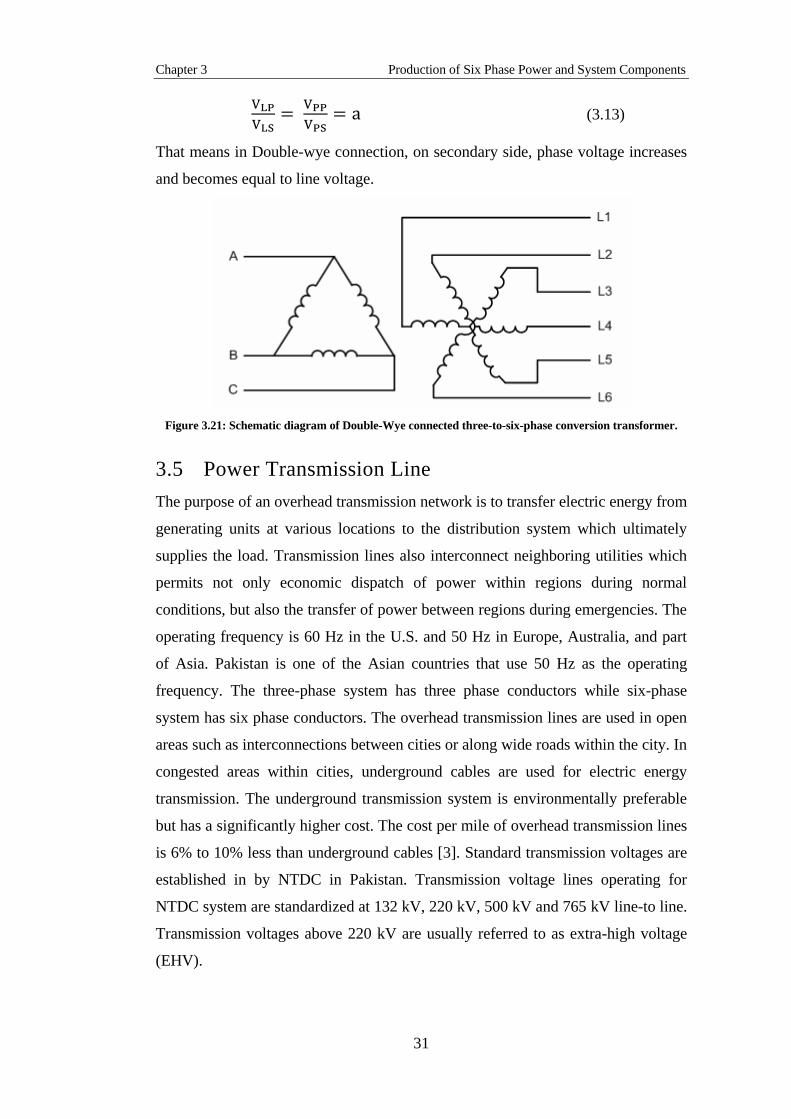
Chapter 3 Production of Six Phase Power and System Components
31
(3.13)
That means in Double-wye connection, on secondary side, phase voltage increases
and becomes equal to line voltage.
Figure 3.21: Schematic diagram of Double-Wye connected three-to-six-phase conversion transformer.
3.5 Power Transmission Line
The purpose of an overhead transmission network is to transfer electric energy from
generating units at various locations to the distribution system which ultimately
supplies the load. Transmission lines also interconnect neighboring utilities which
permits not only economic dispatch of power within regions during normal
conditions, but also the transfer of power between regions during emergencies. The
operating frequency is 60 Hz in the U.S. and 50 Hz in Europe, Australia, and part
of Asia. Pakistan is one of the Asian countries that use 50 Hz as the operating
frequency. The three-phase system has three phase conductors while six-phase
system has six phase conductors. The overhead transmission lines are used in open
areas such as interconnections between cities or along wide roads within the city. In
congested areas within cities, underground cables are used for electric energy
transmission. The underground transmission system is environmentally preferable
but has a significantly higher cost. The cost per mile of overhead transmission lines
is 6% to 10% less than underground cables [3]. Standard transmission voltages are
established in by NTDC in Pakistan. Transmission voltage lines operating for
NTDC system are standardized at 132 kV, 220 kV, 500 kV and 765 kV line-to line.
Transmission voltages above 220 kV are usually referred to as extra-high voltage
(EHV).
Chapter 3 Production of Six Phase Power and System Components
32
A three-phase double-circuit AC system is used for most transmission lines. This
will make the idea of transmitting power using six-phase transmission system much
easier because six conductors of three-phase double-circuit transmission line can be
converted to six-phase transmission line. Conversion of an existing three-phase
double-circuit overhead transmission line to a six-phase operation needed phase
conversion transformers to obtain the 60° phase shift between adjacent phases. A
three-phase double-circuit transmission line can be easily converted to a six-phase
transmission line by using three-to-six-phase conversion transformer. There are
several combinations of identical three-phase transformers that can be used to form
three-to-six-phase and six-to-three-phase conversion transformers. However, the
most suitable one is by using two pairs of identical delta-wye three-phase
transformers. One of each pair of transformers has reverse polarity to obtain the
required 60° phase shift. This combination were selected as appropriate for
determining short circuit currents because the delta open circuits the zero sequence
network and simplifies the fault analysis [15]. For the reason of this fact, three-to-
six- phase and six-to-three-phase conversion transformers that forms by using this
combination has been used throughout this study.
This section will discuss the concepts of surge impedance and surge impedance
loading for lossless lines. When line losses are neglected, simpler expression for the
line parameters are obtained and above concepts are more easily understood. Since
transmission and distribution lines for power transfer generally are designed to have
low losses, the equations and concepts shows here can be used for quick and
reasonably accurate hand calculations leading to initial designs. More accurate
calculations can then be made with computer programs for follow-up analysis and
design.
3.5.1 Surge Impedance
System limitations on power flow include among other considerations voltage drop
and stability. A rule of thumb estimate of power-handling capacity of a
transmission line is given by line-surge-impedance loading. For a lossless line, R =
G = 0. Moreover, these will give the impedance and admittance as follows [3]:
z = jωL Ω/m (3.14)
y = jωC Ω/m (3.15)
Characteristic impedance Zc is given by [3]:
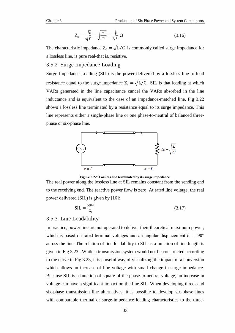
Chapter 3 Production of Six Phase Power and System Components
33
√
√
√
(3.16)
The characteristic impedance √ ⁄ is commonly called surge impedance for
a lossless line, is pure real-that is, resistive.
3.5.2 Surge Impedance Loading
Surge Impedance Loading (SIL) is the power delivered by a lossless line to load
resistance equal to the surge impedance √ ⁄ . SIL is that loading at which
VARs generated in the line capacitance cancel the VARs absorbed in the line
inductance and is equivalent to the case of an impedance-matched line. Fig 3.22
shows a lossless line terminated by a resistance equal to its surge impedance. This
line represents either a single-phase line or one phase-to-neutral of balanced three-
phase or six-phase line.
Figure 3.22: Lossless line terminated by its surge impedance.
The real power along the lossless line at SIL remains constant from the sending end
to the receiving end. The reactive power flow is zero. At rated line voltage, the real
power delivered (SIL) is given by [16]:
(3.17)
3.5.3 Line Loadability
In practice, power line are not operated to deliver their theoretical maximum power,
which is based on rated terminal voltages and an angular displacement δ = 90°
across the line. The relation of line loadability to SIL as a function of line length is
given in Fig 3.23. While a transmission system would not be constructed according
to the curve in Fig 3.23, it is a useful way of visualizing the impact of a conversion
which allows an increase of line voltage with small change in surge impedance.
Because SIL is a function of square of the phase-to-neutral voltage, an increase in
voltage can have a significant impact on the line SIL. When developing three- and
six-phase transmission line alternatives, it is possible to develop six-phase lines
with comparable thermal or surge-impedance loading characteristics to the three-
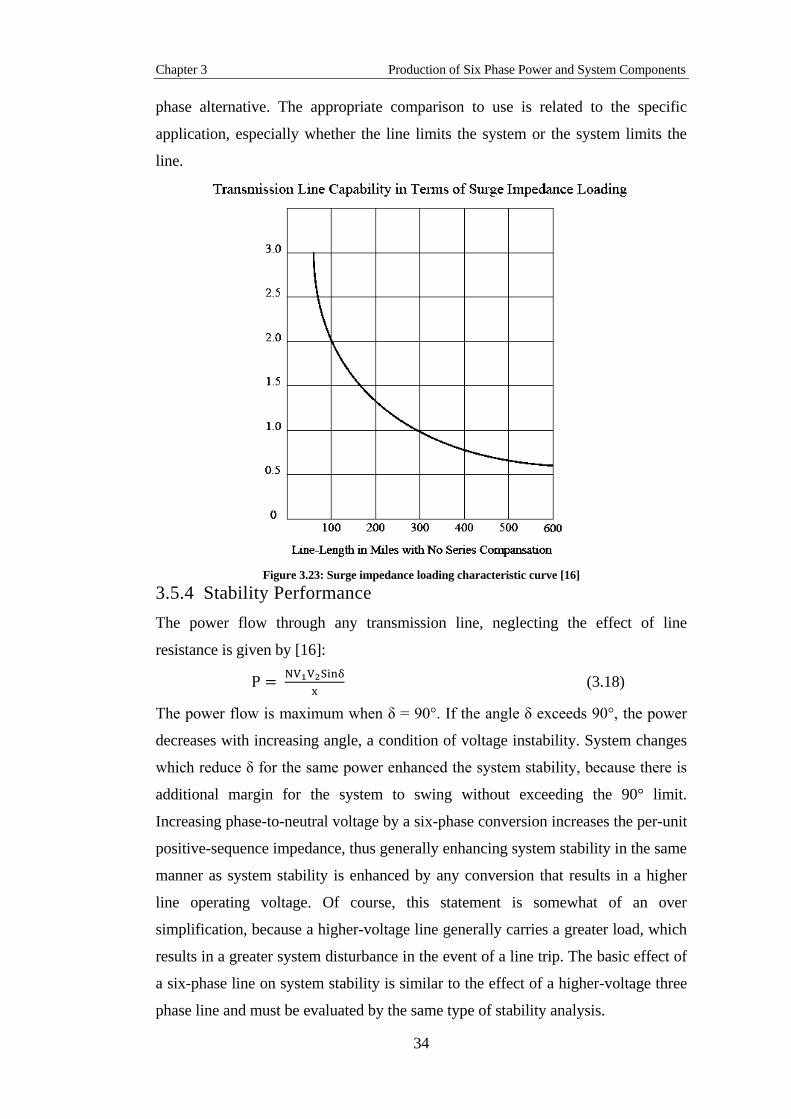
Chapter 3 Production of Six Phase Power and System Components
34
phase alternative. The appropriate comparison to use is related to the specific
application, especially whether the line limits the system or the system limits the
line.
Figure 3.23: Surge impedance loading characteristic curve [16]
3.5.4 Stability Performance
The power flow through any transmission line, neglecting the effect of line
resistance is given by [16]:
(3.18)
The power flow is maximum when δ = 90°. If the angle δ exceeds 90°, the power
decreases with increasing angle, a condition of voltage instability. System changes
which reduce δ for the same power enhanced the system stability, because there is
additional margin for the system to swing without exceeding the 90° limit.
Increasing phase-to-neutral voltage by a six-phase conversion increases the per-unit
positive-sequence impedance, thus generally enhancing system stability in the same
manner as system stability is enhanced by any conversion that results in a higher
line operating voltage. Of course, this statement is somewhat of an over
simplification, because a higher-voltage line generally carries a greater load, which
results in a greater system disturbance in the event of a line trip. The basic effect of
a six-phase line on system stability is similar to the effect of a higher-voltage three
phase line and must be evaluated by the same type of stability analysis.

Chapter 3 Production of Six Phase Power and System Components
35
3.6 Summary
This chapter deal with the components in involved in Six-phase transmission
system. Methods of production of six-phase have been discussed followed by a
detailed analysis of three to six-phase conversion transformers. Voltage
relationships of primary (three-phase side) and secondary (six-phase side) of the
conversion transformers are also derived. In the end, the theoretical aspects
involved in the conversion of a three-phase transmission line to a six-phase
transmission line have been viewed.
Chapter 4 Modeling of six-phase Transmission System in MATLAB®
36
Chapter 4
Modeling of six-phase Transmission
System in MATLAB®
4.1 The Role of Simulation in Design
Electrical power systems are combinations of electrical circuits and
electromechanical devices like motors and generators. Engineers working in this
discipline are constantly improving the performance of the systems. Requirements
for drastically increased efficiency have forced power system designers to use
power electronic devices and sophisticated control system concepts that tax
traditional analysis tools and techniques. Further complicating the analyst's role is
the fact that the system is often so nonlinear that the only way to understand it is
through simulation.
Land-based power generation from hydroelectric, steam, or other devices is not the
only use of power systems. A common attribute of these systems is their use of
power electronics and control systems to achieve their performance objectives.
4.2 SimPowerSystems
SimPowerSystems software is a modern design tool that allows scientists and
engineers to rapidly and easily build models that simulate power systems. It uses
the Simulink environment, allowing you to build a model using simple click and
drag procedures. Not only can you draw the circuit topology rapidly, but your
analysis of the circuit can include its interactions with mechanical, thermal, control,
and other disciplines. This is possible because all the electrical parts of the
simulation interact with the extensive Simulink modeling library. Since Simulink
uses the MATLAB® computational engine, designers can also use MATLAB®
Chapter 4 Modeling of six-phase Transmission System in MATLAB®
37
toolboxes and Simulink block-sets. SimPowerSystems software belongs to the
Physical Modeling product family and uses similar block and connection line
interface.
4.2.1 Simulation and Model-Based Design
Simulink® is an environment for multi domain simulation and Model-Based
Design for dynamic and embedded systems. It provides an interactive graphical
environment and a customizable set of block libraries that let you design, simulate,
implement, and test a variety of time-varying systems, including communications,
controls, signal processing, video processing, and image processing.
Following are the Key Features of Simulink®:
Extensive and expandable libraries of predefined blocks
Interactive graphical editor for assembling and managing intuitive block
diagrams
Ability to manage complex designs by segmenting models into hierarchies
of design components
Model Explorer to navigate, create, configure, and search all signals,
parameters, properties, and generated code associated with your model
Application programming interfaces (APIs) that let you connect with other
simulation programs and incorporate hand-written code
MATLAB® Function blocks for bringing MATLAB algorithms into
Simulink and embedded system implementations
Graphical debugger and profiler to examine simulation results and then
diagnose performance and unexpected behavior in your design
4.2.2 Model and simulate electrical power systems
SimPowerSystems provides component libraries for modeling and simulating
electrical power systems. It includes models of three-phase machines, electric
drives, flexible AC transmission systems (FACTS), and wind power generators.
Abstracted models of power electronics components are also included, enabling
you to assess the impact of switching events on system-level behavior. You can use
these components to model the generation, transmission, distribution, and
consumption of electrical power.
Chapter 4 Modeling of six-phase Transmission System in MATLAB®
38
Harmonic analysis, calculation of total harmonic distortion (THD), load flow, and
other key electrical power system analyses are automated. SimPowerSystems
models can be discretized to speed up simulations and configured for phasor
simulation, which helps you determine the transient stability of electrical power
systems.
Key Features of SimPowerSystems are [17]:
Application-specific models, including common AC and DC electric drives,
flexible AC transmission systems, and wind-power generators
Ideal switching algorithm for fast simulation of power electronic devices
Functions for obtaining equivalent state-space representations of circuits
Tools for computing load flow and for initializing models of three-phase
networks with machines
Demonstration models of key electrical technologies
4.3 Overview of SimPowerSystems Libraries
SimPowerSystems libraries contain models of typical power equipment such as
transformers, lines, machines, and power electronics. These models are proven ones
coming from textbooks, and their validity is based on the experience of the Power
Systems Testing and Simulation Laboratory of Hydro-Québec, a large North
American utility located in Canada, and also on the experience of École de
Technologie Supérieure and Université Laval. The capabilities of
SimPowerSystems software for modeling a typical electrical system are illustrated
in demonstration files. And for users who want to refresh their knowledge of power
system theory, there are also self-learning case studies. [17]
The SimPowerSystems main library, powerlib, organizes its blocks into libraries
according to their behavior. To open this library, type powerlib in the MATLAB®
Command Window. The powerlib library window displays the block library icons
and names. Double-click a library icon to open the library and access the blocks.
The main powerlib library window also contains the Powergui block that opens a
graphical user interface for the steady-state analysis of electrical circuits.
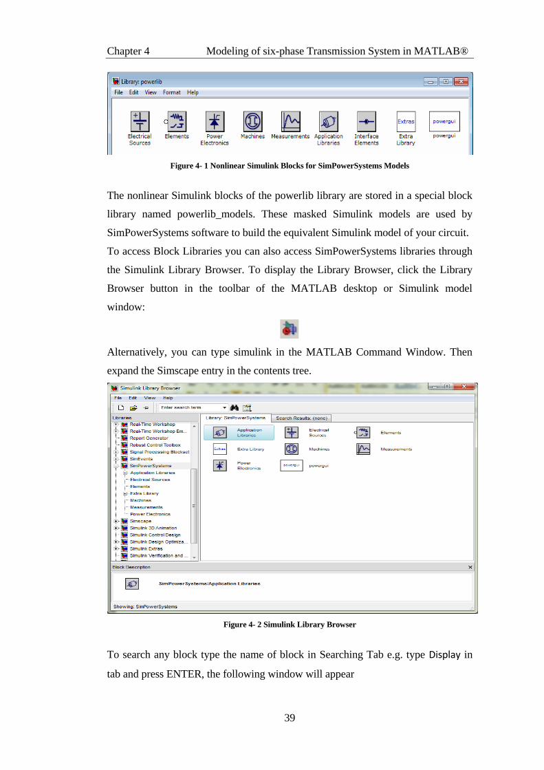
Chapter 4 Modeling of six-phase Transmission System in MATLAB®
39
Figure 4- 1 Nonlinear Simulink Blocks for SimPowerSystems Models
The nonlinear Simulink blocks of the powerlib library are stored in a special block
library named powerlib_models. These masked Simulink models are used by
SimPowerSystems software to build the equivalent Simulink model of your circuit.
To access Block Libraries you can also access SimPowerSystems libraries through
the Simulink Library Browser. To display the Library Browser, click the Library
Browser button in the toolbar of the MATLAB desktop or Simulink model
window:
Alternatively, you can type simulink in the MATLAB Command Window. Then
expand the Simscape entry in the contents tree.
Figure 4- 2 Simulink Library Browser
To search any block type the name of block in Searching Tab e.g. type Display in
tab and press ENTER, the following window will appear

Chapter 4 Modeling of six-phase Transmission System in MATLAB®
40
Figure 4- 3 Display block for numeric display of input values
Select your desired element and connect it in the system.
4.4 Modeling of Three-phase double circuit line on
Simulink
First of all, a model of three-phase double circuit line was built in Simulink. A three
phase source at voltage level of 220kV was taken and then it was stepped up, up to
500kV and also converting it to double circuit line by using transformation block as
shown in fig.4.4. Fig.4.5 shows the internal connections of the transformation
block.
Figure 4-4 Block diagram of Three phase transformer
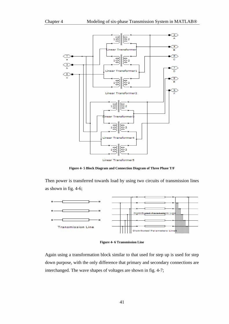
Chapter 4 Modeling of six-phase Transmission System in MATLAB®
41
Figure 4- 5 Block Diagram and Connection Diagram of Three Phase T/F
Then power is transferred towards load by using two circuits of transmission lines
as shown in fig. 4-6;
Figure 4- 6 Transmission Line
Again using a transformation block similar to that used for step up is used for step
down purpose, with the only difference that primary and secondary connections are
interchanged. The wave shapes of voltages are shown in fig. 4-7;
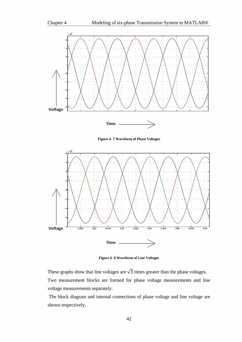
Chapter 4 Modeling of six-phase Transmission System in MATLAB®
42
Figure 4- 7 Waveform of Phase Voltages
Figure 4- 8 Waveform of Line Voltages
These graphs show that line voltages are √ times greater than the phase voltages.
Two measurement blocks are formed for phase voltage measurements and line
voltage measurements separately.
The block diagram and internal connections of phase voltage and line voltage are
shown respectively.
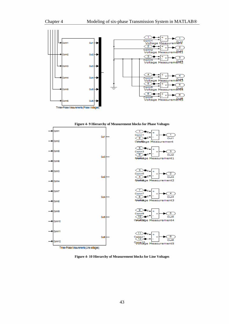
Chapter 4 Modeling of six-phase Transmission System in MATLAB®
43
Figure 4- 9 Hierarchy of Measurement blocks for Phase Voltages
Figure 4- 10 Hierarchy of Measurement blocks for Line Voltages

Chapter 4 Modeling of six-phase Transmission System in MATLAB®
44
Figure 4- 11 Complete model of Three Phase double circuit Transmission System
The line current is almost 156A. For this modal of power system a Three-Phase
RLC load of following settings is used
Figure 4- 12 Three-Phase RLC load
4.5 Modeling of six phase transmission system

Chapter 4 Modeling of six-phase Transmission System in MATLAB®
45
Power system model for six phase transmission lines is similar to that shown in
figure 4-10 but the only difference here is that connections of transformers in
transformation blocks are such that three phase voltages of source are stepped up
and are also converted into six phase and all the phases are equally displaced from
each other i.e. at an angle of 60°.
There are different transformer configurations used for this type of conversion and
these configurations are shown in the table 4.1 [18].
Type of Connection Schematic Diagram
Wye-Wye
Wye-Inverted-Y
Delta-Wye
Delta Inverted-Y
Diametrical

Chapter 4 Modeling of six-phase Transmission System in MATLAB®
46
Double Delta
Double Wye
Table 4.1
4.5.1 Transformation block for wye-wye wye-inverted-wye
The internal configuration of six single phase transformers in transformation block
of power system is shown in fig. 4-13
Figure 4- 13 Y-Y Y-Inverted Y Configuration of Transformers
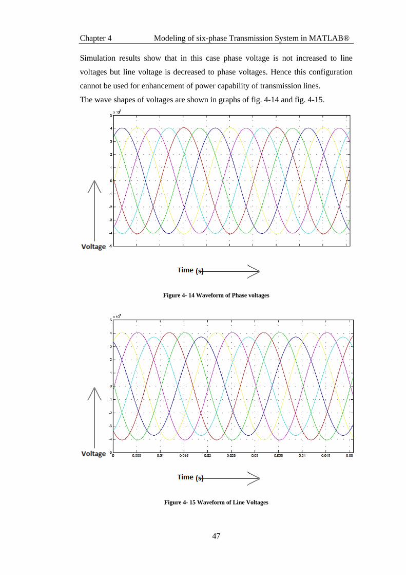
Chapter 4 Modeling of six-phase Transmission System in MATLAB®
47
Simulation results show that in this case phase voltage is not increased to line
voltages but line voltage is decreased to phase voltages. Hence this configuration
cannot be used for enhancement of power capability of transmission lines.
The wave shapes of voltages are shown in graphs of fig. 4-14 and fig. 4-15.
Figure 4- 14 Waveform of Phase voltages
Figure 4- 15 Waveform of Line Voltages
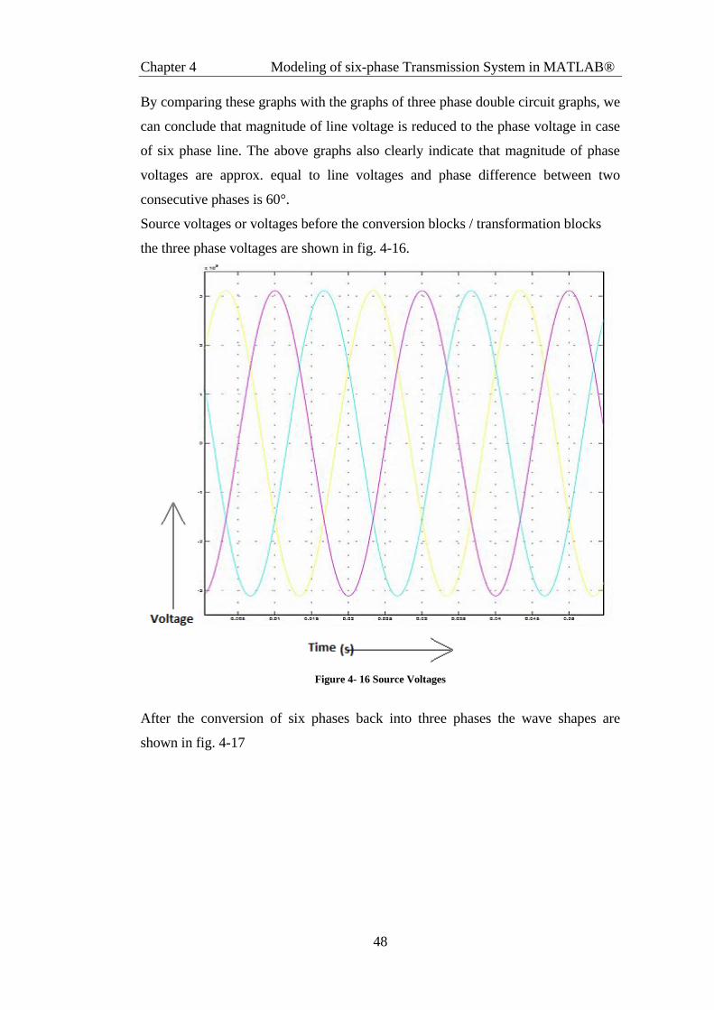
Chapter 4 Modeling of six-phase Transmission System in MATLAB®
48
By comparing these graphs with the graphs of three phase double circuit graphs, we
can conclude that magnitude of line voltage is reduced to the phase voltage in case
of six phase line. The above graphs also clearly indicate that magnitude of phase
voltages are approx. equal to line voltages and phase difference between two
consecutive phases is 60°.
Source voltages or voltages before the conversion blocks / transformation blocks
the three phase voltages are shown in fig. 4-16.
Figure 4- 16 Source Voltages
After the conversion of six phases back into three phases the wave shapes are
shown in fig. 4-17

Chapter 4 Modeling of six-phase Transmission System in MATLAB®
49
Figure 4- 17 Voltages across Load
The overall power system modeling is shown in fig. 4-18.
Figure 4-18 Complete System for Six Phase Transmission Using Y-Y, Y-Inverted Y Transformer
configuration
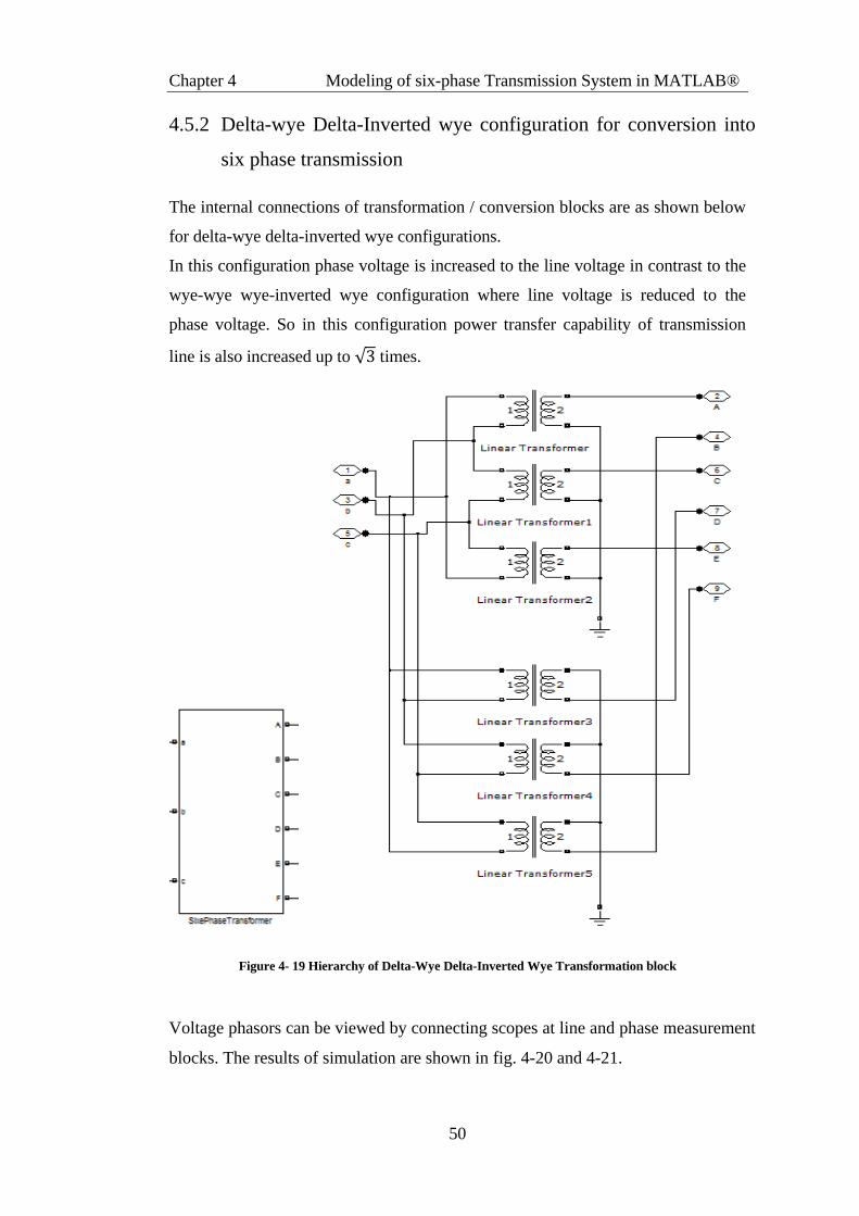
Chapter 4 Modeling of six-phase Transmission System in MATLAB®
50
4.5.2 Delta-wye Delta-Inverted wye configuration for conversion into
six phase transmission
The internal connections of transformation / conversion blocks are as shown below
for delta-wye delta-inverted wye configurations.
In this configuration phase voltage is increased to the line voltage in contrast to the
wye-wye wye-inverted wye configuration where line voltage is reduced to the
phase voltage. So in this configuration power transfer capability of transmission
line is also increased up to √ times.
Figure 4- 19 Hierarchy of Delta-Wye Delta-Inverted Wye Transformation block
Voltage phasors can be viewed by connecting scopes at line and phase measurement
blocks. The results of simulation are shown in fig. 4-20 and 4-21.
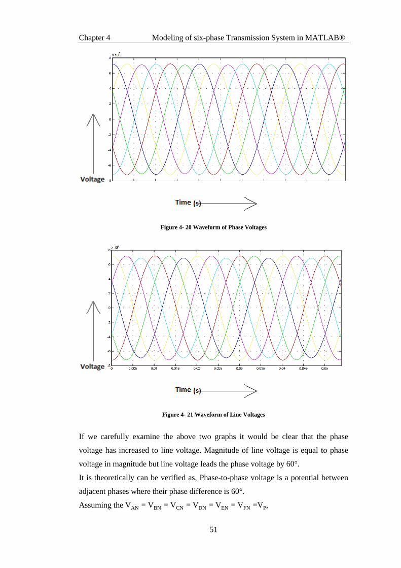
Chapter 4 Modeling of six-phase Transmission System in MATLAB®
51
Figure 4- 20 Waveform of Phase Voltages
Figure 4- 21 Waveform of Line Voltages
If we carefully examine the above two graphs it would be clear that the phase
voltage has increased to line voltage. Magnitude of line voltage is equal to phase
voltage in magnitude but line voltage leads the phase voltage by 60°.
It is theoretically can be verified as, Phase-to-phase voltage is a potential between
adjacent phases where their phase difference is 60°.
Assuming the VAN = VBN = VCN = VDN = VEN = VFN =VP,
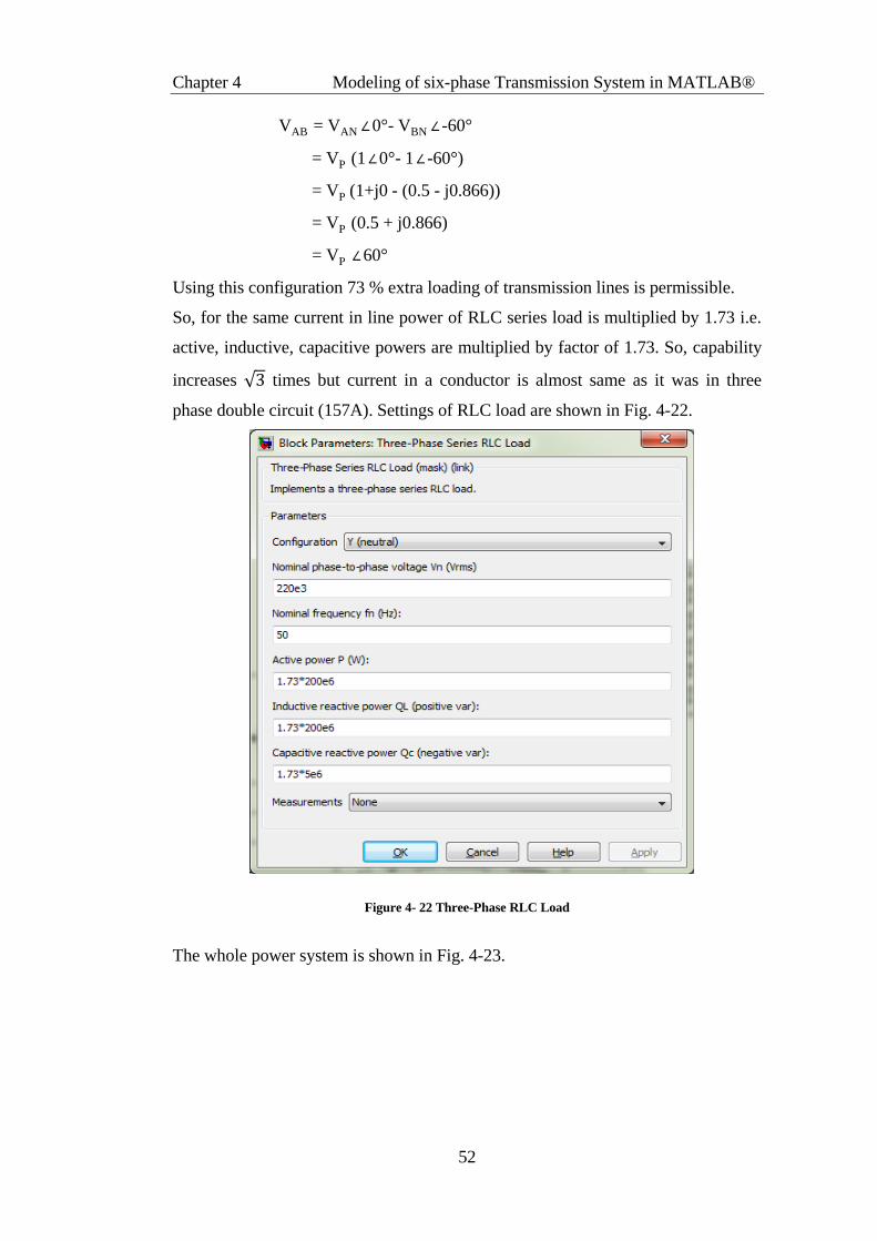
Chapter 4 Modeling of six-phase Transmission System in MATLAB®
52
VAB = VAN ∠ 0°- VBN ∠ -60°
= VP (1 ∠ 0°- 1 ∠ -60°)
= VP (1+j0 - (0.5 - j0.866))
= VP (0.5 + j0.866)
= VP ∠ 60°
Using this configuration 73 % extra loading of transmission lines is permissible.
So, for the same current in line power of RLC series load is multiplied by 1.73 i.e.
active, inductive, capacitive powers are multiplied by factor of 1.73. So, capability
increases √ times but current in a conductor is almost same as it was in three
phase double circuit (157A). Settings of RLC load are shown in Fig. 4-22.
Figure 4- 22 Three-Phase RLC Load
The whole power system is shown in Fig. 4-23.
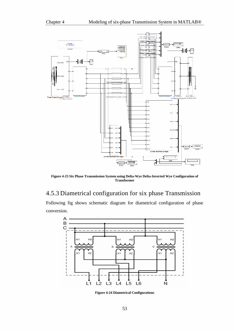
Chapter 4 Modeling of six-phase Transmission System in MATLAB®
53
Figure 4-23 Six Phase Transmission System using Delta-Wye Delta-Inverted Wye Configuration of
Transformer
4.5.3 Diametrical configuration for six phase Transmission
Following fig shows schematic diagram for diametrical configuration of phase
conversion.
Figure 4-24 Diametrical Configurations
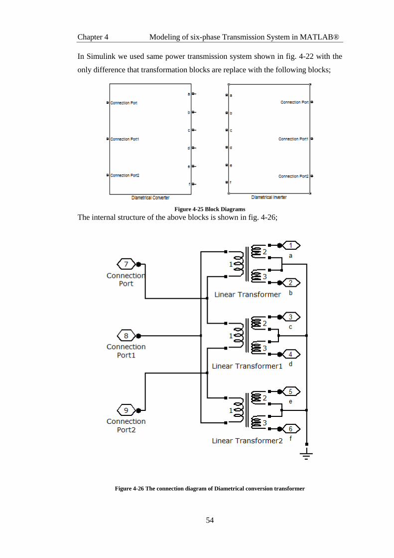
Chapter 4 Modeling of six-phase Transmission System in MATLAB®
54
In Simulink we used same power transmission system shown in fig. 4-22 with the
only difference that transformation blocks are replace with the following blocks;
Figure 4-25 Block Diagrams
The internal structure of the above blocks is shown in fig. 4-26;
Figure 4-26 The connection diagram of Diametrical conversion transformer
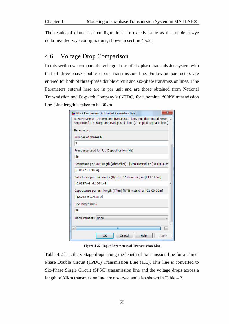
Chapter 4 Modeling of six-phase Transmission System in MATLAB®
55
The results of diametrical configurations are exactly same as that of delta-wye
delta-inverted-wye configurations, shown in section 4.5.2.
4.6 Voltage Drop Comparison
In this section we compare the voltage drops of six-phase transmission system with
that of three-phase double circuit transmission line. Following parameters are
entered for both of three-phase double circuit and six-phase transmission lines. Line
Parameters entered here are in per unit and are those obtained from National
Transmission and Dispatch Company’s (NTDC) for a nominal 500kV transmission
line. Line length is taken to be 30km.
Figure 4-27: Input Parameters of Transmission Line
Table 4.2 lists the voltage drops along the length of transmission line for a Three-
Phase Double Circuit (TPDC) Transmission Line (T.L). This line is converted to
Six-Phase Single Circuit (SPSC) transmission line and the voltage drops across a
length of 30km transmission line are observed and also shown in Table 4.3.
Chapter 4 Modeling of six-phase Transmission System in MATLAB®
56
Table 4.2: Voltage Drop across the length of transmission lines for three-phase and six-phase with 73%
extra load.
Sr. No. Phase SPSC T.L Voltage Drop TPDC T.L Voltage Drop
1 A/A 3342 Vrms 1249 Vrms
2 B/B 4177 Vrms 1249 Vrms
3 C/C 3961 Vrms 1249 Vrms
4 D/A’ 3342 Vrms 1249 Vrms
5 E/B’ 4177 Vrms 1249 Vrms
6 F/C’ 3961 Vrms 1249 Vrms
It is quite easily observable that the voltage drops in six-phase transmission line are
greater than those in three-phase double circuit transmission line. This may be due
to the increased load i.e 1.73 times that of three phase double circuit transmission
line. To verify, we have again listed the voltage drops in six-phase transmission line
that are due the line with same load as that of three-phase double circuit line.
Table 4.3 lists the voltage drops across a 30km long 500kV three phase double
circuit and six-phase transmission line for the same load.
This table verifies that the voltage drop across the six-phase transmission line is
greater than that of three-phase double circuit transmission line that is a demerit of
six phase transmission line.
Table 4.3: Voltage drops across the length of transmission line for Six phase with same load as three-
phase.
Sr. No. Phase SPSC T.L Voltage Drop TPDC T.L Voltage Drop
1 A/A 1862 Vrms 1249 Vrms
2 B/B 2366 Vrms 1249 Vrms
3 C/C 2261 Vrms 1249 Vrms
4 D/A’ 1862 Vrms 1249 Vrms
5 E/B’ 2366 Vrms 1249 Vrms
6 F/C’ 2261 Vrms 1249 Vrms
So we note here that the six-phase power transmission line has poor voltage
regulation than that of three-phase double circuit transmission line.
4.7 Summary
In this chapter modeling and comparison of three-phase double circuit and six-
phase single circuit transmission lines are performed in Simulink/MATLAB®.
Quantity of power flow or power transfer capability and voltage drops for both the
transmission line is compared.
Chapter 5 Electromagnetic Field Gradients
57
Chapter 5
Electromagnetic Field Gradients
In the recent era the, construction of new electrical power transmission lines are
strongly constrained by the Right of Way Requirement. Increasing cost of land and
legal issues involved in the acquiring land have compelled electric design engineers
to look for alternatives to transmit power to the distribution stations.
One of the major advantages of six-phase transmission is less ROW requirement.
The up-gradation of existing three-phase double circuit transmission line to six-
phase transmission line eliminates the construction of new line and hence ROW
requirement. Moreover, the construction of new six-phase transmission line using
compact structures requires less land for its construction. ROW requirement
directly depends upon the size of tower structures and electromagnetic field limits
imposed by the Environment Safety Authorities. Both of these elements directly
depend on the electric and magnetic field gradients around a transmission line.
In this chapter we analyze the Electric and Magnetic field across a Six-phase
transmission line and compare it with the three-phase double circuit transmission
line under same tower structures. A MATLAB program has been developed for the
calculation and plotting of Six-phase transmission line electric and magnetic field.
Now we start from calculating the magnetic field. Basic definitions and equations
are described first followed by the case study of six-phase transmission line.
5.1 Magnetic Field Basics
An electric charge has an electric field, while an electric current produces a
magnetic field. The magnetic field is considered as static in case of DC
transmission and quasi-static in the case of AC transmission lines. In the calculation
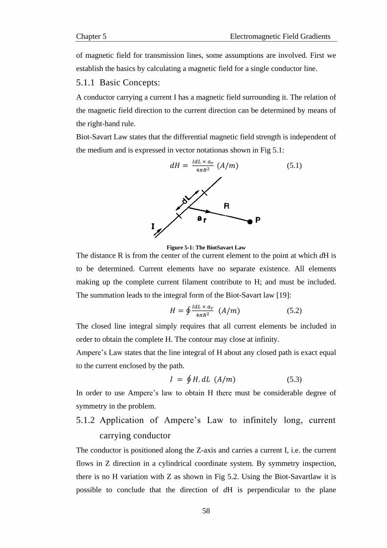
Chapter 5 Electromagnetic Field Gradients
58
of magnetic field for transmission lines, some assumptions are involved. First we
establish the basics by calculating a magnetic field for a single conductor line.
5.1.1 Basic Concepts:
A conductor carrying a current I has a magnetic field surrounding it. The relation of
the magnetic field direction to the current direction can be determined by means of
the right-hand rule.
Biot-Savart Law states that the differential magnetic field strength is independent of
the medium and is expressed in vector notationas shown in Fig 5.1:
(5.1)
Figure 5-1: The BiotSavart Law
The distance R is from the center of the current element to the point at which dH is
to be determined. Current elements have no separate existence. All elements
making up the complete current filament contribute to H; and must be included.
The summation leads to the integral form of the Biot-Savart law [19]:
∮
(5.2)
The closed line integral simply requires that all current elements be included in
order to obtain the complete H. The contour may close at infinity.
Ampere’s Law states that the line integral of H about any closed path is exact equal
to the current enclosed by the path.
∮ (5.3)
In order to use Ampere’s law to obtain H there must be considerable degree of
symmetry in the problem.
5.1.2 Application of Ampere’s Law to infinitely long, current
carrying conductor
The conductor is positioned along the Z-axis and carries a current I, i.e. the current
flows in Z direction in a cylindrical coordinate system. By symmetry inspection,
there is no H variation with Z as shown in Fig 5.2. Using the Biot-Savartlaw it is
possible to conclude that the direction of dH is perpendicular to the plane
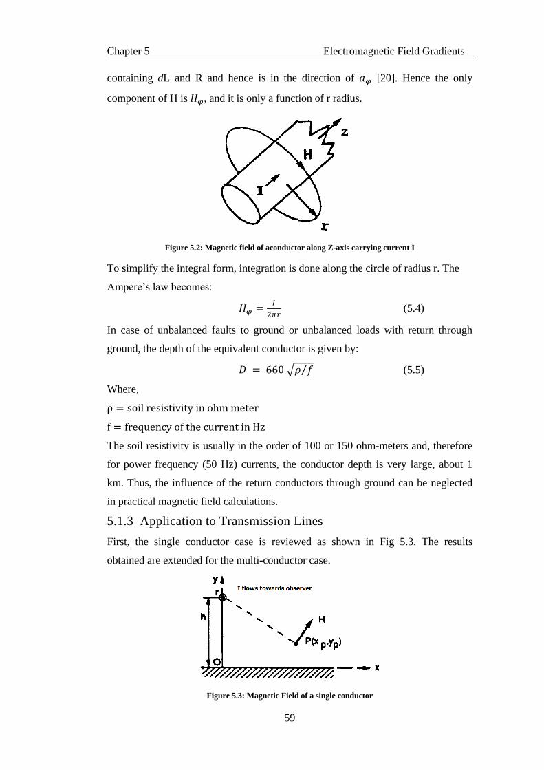
Chapter 5 Electromagnetic Field Gradients
59
containing dL and R and hence is in the direction of [20]. Hence the only
component of H is , and it is only a function of r radius.
Figure 5.2: Magnetic field of aconductor along Z-axis carrying current I
To simplify the integral form, integration is done along the circle of radius r. The
Ampere’s law becomes:
(5.4)
In case of unbalanced faults to ground or unbalanced loads with return through
ground, the depth of the equivalent conductor is given by:
√ ⁄ (5.5)
Where,
The soil resistivity is usually in the order of 100 or 150 ohm-meters and, therefore
for power frequency (50 Hz) currents, the conductor depth is very large, about 1
km. Thus, the influence of the return conductors through ground can be neglected
in practical magnetic field calculations.
5.1.3 Application to Transmission Lines
First, the single conductor case is reviewed as shown in Fig 5.3. The results
obtained are extended for the multi-conductor case.
Figure 5.3: Magnetic Field of a single conductor

Chapter 5 Electromagnetic Field Gradients
60
If current I is given as a phasor, then Eq. 5.4 can be used:
| |
(5.6)
√
(5.7)
| |
(5.8)
| |
(5.9)
In case of a multi-conductor line, i represents the conductor number and Iirepresents
the current in conductor i as a phasor as shown in Fig 5.4.[19]
Figure 5.4: Magnetic field of a multi-conductor line
∑
(5.10)
∑
√
(5.11)
∑
∑
(5.12)
∑
∑
(5.13)
| | √
(5.14)
Eq. 5.14 gives the magnitude of the electric field strength vector. This equation can
be plotted against the points (xp,yp) to have a graphical picture of the magnetic
field.
5.1.4 Computer Program for calculation of Magnetic Fields
A program in MATLAB is written for the calculation of magnetic field. The input
to the program is the geometry of the tower, current magnitudes with phasors and
the space (set of points) in which the magnetic field is to be evaluated. The output
of the program is the value of magnetic field strength, a plot of magnetic field
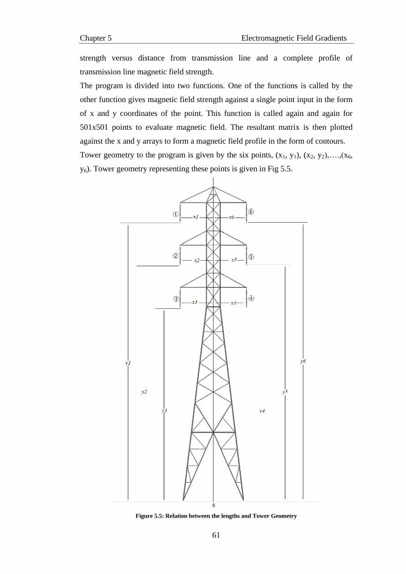
Chapter 5 Electromagnetic Field Gradients
61
strength versus distance from transmission line and a complete profile of
transmission line magnetic field strength.
The program is divided into two functions. One of the functions is called by the
other function gives magnetic field strength against a single point input in the form
of x and y coordinates of the point. This function is called again and again for
501x501 points to evaluate magnetic field. The resultant matrix is then plotted
against the x and y arrays to form a magnetic field profile in the form of contours.
Tower geometry to the program is given by the six points, (x1, y1), (x2, y2),….,(x6,
y6). Tower geometry representing these points is given in Fig 5.5.
Figure 5.5: Relation between the lengths and Tower Geometry
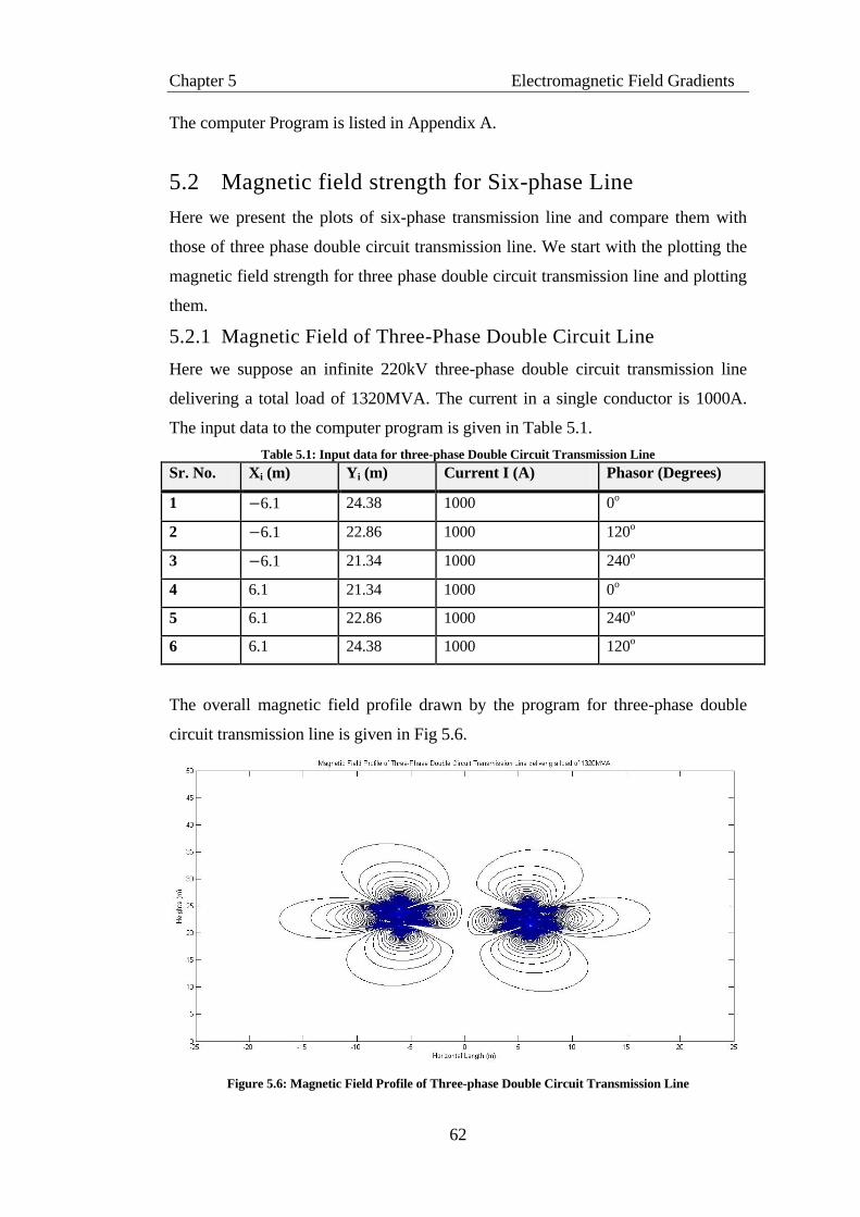
Chapter 5 Electromagnetic Field Gradients
62
The computer Program is listed in Appendix A.
5.2 Magnetic field strength for Six-phase Line
Here we present the plots of six-phase transmission line and compare them with
those of three phase double circuit transmission line. We start with the plotting the
magnetic field strength for three phase double circuit transmission line and plotting
them.
5.2.1 Magnetic Field of Three-Phase Double Circuit Line
Here we suppose an infinite 220kV three-phase double circuit transmission line
delivering a total load of 1320MVA. The current in a single conductor is 1000A.
The input data to the computer program is given in Table 5.1.
Table 5.1: Input data for three-phase Double Circuit Transmission Line
Sr. No. Xi (m) Yi (m) Current I (A) Phasor (Degrees)
1 6.1 24.38 1000 0o
2 6.1 22.86 1000 120o
3 6.1 21.34 1000 240o
4 6.1 21.34 1000 0o
5 6.1 22.86 1000 240o
6 6.1 24.38 1000 120o
The overall magnetic field profile drawn by the program for three-phase double
circuit transmission line is given in Fig 5.6.
Figure 5.6: Magnetic Field Profile of Three-phase Double Circuit Transmission Line
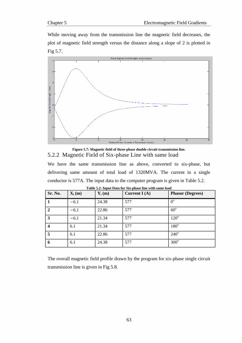
Chapter 5 Electromagnetic Field Gradients
63
While moving away from the transmission line the magnetic field decreases, the
plot of magnetic field strength versus the distance along a slope of 2 is plotted in
Fig 5.7.
Figure 5.7: Magnetic field of three-phase double circuit transmission line.
5.2.2 Magnetic Field of Six-phase Line with same load
We have the same transmission line as above, converted to six-phase, but
delivering same amount of total load of 1320MVA. The current in a single
conductor is 577A. The input data to the computer program is given in Table 5.2.
Table 5.2: Input Data for Six-phase line with same load
Sr. No. Xi (m) Yi (m) Current I (A) Phasor (Degrees)
1 6.1 24.38 577 0o
2 6.1 22.86 577 60o
3 6.1 21.34 577 120o
4 6.1 21.34 577 180o
5 6.1 22.86 577 240o
6 6.1 24.38 577 300o
The overall magnetic field profile drawn by the program for six-phase single circuit
transmission line is given in Fig 5.8.
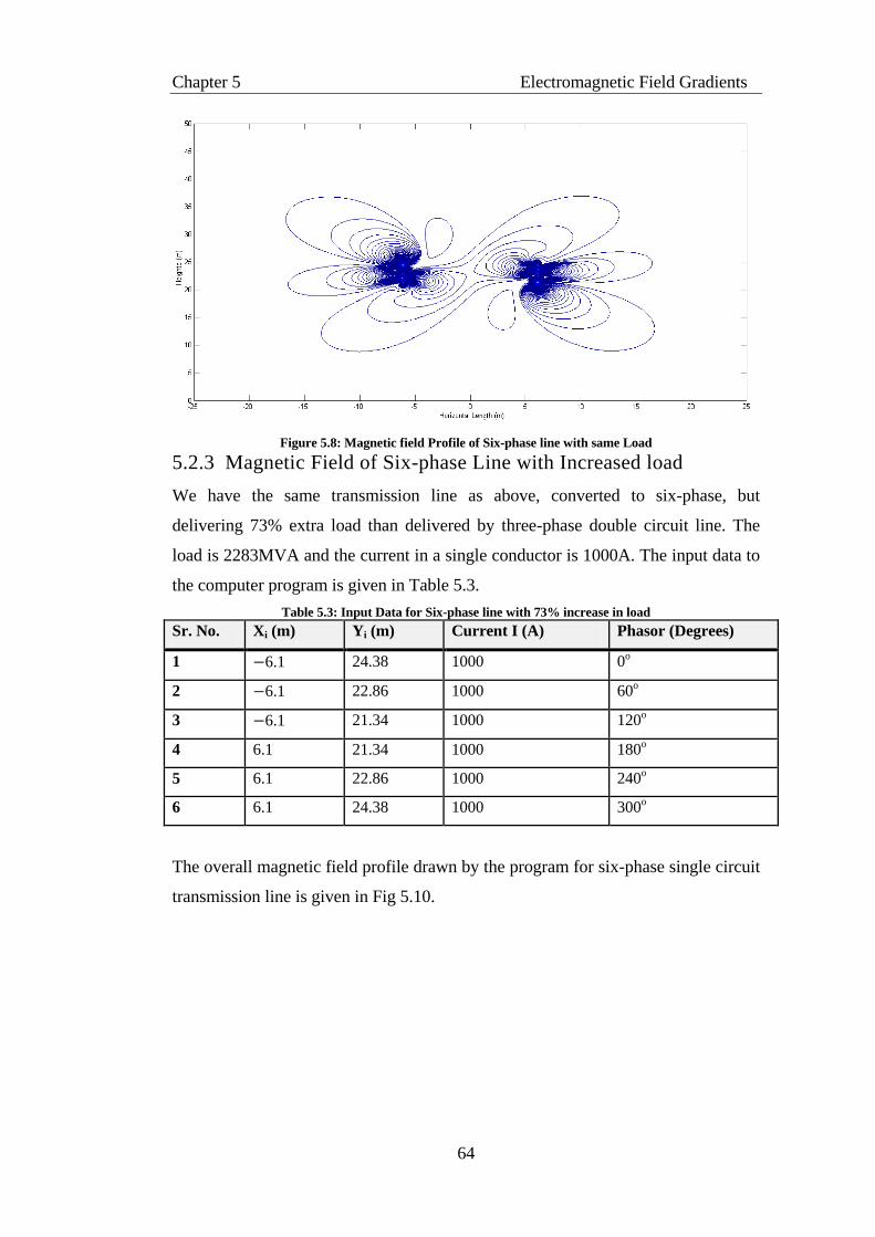
Chapter 5 Electromagnetic Field Gradients
64
Figure 5.8: Magnetic field Profile of Six-phase line with same Load
5.2.3 Magnetic Field of Six-phase Line with Increased load
We have the same transmission line as above, converted to six-phase, but
delivering 73% extra load than delivered by three-phase double circuit line. The
load is 2283MVA and the current in a single conductor is 1000A. The input data to
the computer program is given in Table 5.3.
Table 5.3: Input Data for Six-phase line with 73% increase in load
Sr. No. Xi (m) Yi (m) Current I (A) Phasor (Degrees)
1 6.1 24.38 1000 0o
2 6.1 22.86 1000 60o
3 6.1 21.34 1000 120o
4 6.1 21.34 1000 180o
5 6.1 22.86 1000 240o
6 6.1 24.38 1000 300o
The overall magnetic field profile drawn by the program for six-phase single circuit
transmission line is given in Fig 5.10.

Chapter 5 Electromagnetic Field Gradients
65
Figure 5.9: Magnetic Field Profile of Six-Phase with increased load
While moving away from the transmission line the magnetic field decreases, the
plot of magnetic field strength versus the distance along a slope of 2 is plotted in
Figure 5.10.
Figure 5-10: Plot of Magnetic field of six-phase line
5.2.4 Results and Conclusion
From above plots, following results are obvious:
1. Magnetic field of three-phase double circuit transmission line is
concentrated near the conductors and has greater strength between the
conductors.
2. Magnetic field around six-phase transmission line with same load is less
than three-phase double circuit transmission line.
Chapter 5 Electromagnetic Field Gradients
66
3. Magnetic field strength between the conductors is less for a six-phase
transmission line as compared to that of three-phase double circuit
transmission line.
4. Magnetic Field of a six-phase line with increased load is greater than
magnetic field in three-phase double circuit line. But its strength between
conductors in less than that of three-phase double circuit line.
5. Magnetic field around three-phase double circuit transmission line vanishes
rapidly and disappears completely after a distance of 20m from line.
6. Magnetic field around six-phase line is decreases rapidly in start, and then it
decays slowly, even after 20m from the center of the line it sustains a little
amount of magnetic field strength.
7. Six-phase line magnetic field is less concentrated but sustains long as we
move away from transmission line.
From above statements following conclusions can be made:
1. Magnetic field strength between the conductors of six-phase line is less than
that of three-phase line, so less conductor spacing is required in six-phase
conductors.
2. Magnetic field of the six-phase line sustains a very small value, even after
20m distance from the center of line, but the value is less than 2A/m which
is environmentally safe.
3. So, six-phase transmission line have no trouble in feasibility regarding
magnetic field concerns, but it has a benefit that compact structures can be
made that require less conductor spacing.
5.3 Analysis of transmission line conductor surface
voltage gradients computations
5.3.1 Introduction of Electric fields
The voltage applied to the conductor of a transmission line produce electric field in
the region around the conductor and of course between the conductor and ground.
For DC transmission line the electric field is purely static field in case of AC
transmission line, the electric field is considered as quasi static although they vary
sinusoidally with time at power frequency. Thus the frequency of variation of the
field is sufficiently low to permit the consideration of the electric field

Chapter 5 Electromagnetic Field Gradients
67
independently of each other and calculation on the basis of static field concepts.
The analysis of transmission line conductor surface voltage gradients requires an
understanding of the basic assumption and theorems. Before beginning the study of
electromagnetic fields by investigating those fields that originate from stationary
electric charges, let’s start with coulomb’s law for electrostatic forces because it is
fundamental.
It is used then to derive Laplace’s equation which makes it possible to calculate the
electric field strength and voltage produced by transmission lines one of the most
useful tools used in these. The calculation of the electric field produced by
transmission lines is a complex problem because of the following practical aspects:
conductor sag, proximity of towers, uneven conductor and ground surface, finite
ground conductivity etc. certain basic assumptions are involved in all existing
methods for calculating the electric field in the vicinity of transmission line
conductors.
The ground is assumed to be an infinite, horizontal, conducting plane surface. The
conductors are assumed to be smooth, infinitely long circular cylinders parallel to
each other and to the ground plane. The influence of the conductor support
structures and of any objects in the vicinity of the conductors is neglected. The
horizontal spacing between the conductors remains constant at a specified value
and the height above ground of each conductor is an average value equal to H + 2/3
s, where H is the height above ground at the support point and S is the conductor
sag corresponding to the mean annual temperature.
5.3.2 Basic Equations
It has been found experimentally that the force between two stationary electric
point charges Qa and Qb
a) acts along the line joining the two charges,
b) is proportional to the product Qa*Qb
c) is inversely proportional to the square of the distance ‘’r’’ separating
the charges. The results of this experiment are described by
coulomb’s law and given by:
(5.15)
Where F = force, Newton
= unit vector pointing in direction
Qa, Qb = charges, coulombs

Chapter 5 Electromagnetic Field Gradients
68
= permittivity of the medium, farads/meter
r = distance between charges, meters
The interaction between point charges and in coulomb’s law can be
consiered as an interaction between and the field of or vice versa.The
electric filed intensity E is defined to be the force per unit charge exerted on a test
charge in the field. Thus the electric filed intensity due to the point charge is
⁄ (5.16)
If the electric field is produced by more than one charge each one produces its own
filed, and resultant E is simply the vector sum of the entire individual E’s by the
principle of superposition. Thus
∑
(5.17)
Where is distance from i to a test point where is measured. The direction of E
is defined as pointing away from a positive charge and towards a negative charge as
shown
Figure 5.11: Vector addition of fields due to two charges.
The total field E is the vector addition of field due to individual charges. Consider a
test point charge Q that can be moved from a to b in an electric field E. The electric
potential is defined as the work required moving it per unit charge. It is
proportional to the electric field strength E and to the distance the charge is moved
parallel to the field. That is
∫ ∫ ∫
(5.17)
Referring to the Fig 5.3 is angle between E and
Chapter 5 Electromagnetic Field Gradients
69
In case of a nonuniform field,the electric field E is radial and is inversaly
propotional to squre of the distance r from the source charge.As shown in Fig ,a test
charge is moved from radius r2 to radius r1,from a positive point charge.The
potential difference between the points is given by inseritng Equation (5.16) into
(5.17).
∫
(5.18)
Figure 5.13:Linear path in nonunform electric field
The potential at r1 can be calculated from Equation 5.15 by placing r2 at
infinity.This gives a zero potential at r2 and Equation 5.15 become
(5.19)
This is called the absolute potential of the point due to the charge Q.it was
pointed out in Equation (5.14) that the electric field E is given by the negative rate
Figure 5.12: Potential difference between two points a and b

Chapter 5 Electromagnetic Field Gradients
70
of charge or the negative gradient of potential reduces most rapidly. This statement
is abbreviated to expression E=-grad V or V,
And is called either electric field strength or voltage gradient. The del operator is
then defined as a vector operation. In rectangular coordinates
(5.20)
(5.21)
In cylindrical coordinates
(5.22)
(5.23)
According to gauss’s law the flux of E through a closed surface equals the total
charge enclosed within the surface. Gauss’s law provides us with a powerful
method for calculating the electric field intensity E of simple charge distribution.
Gauss’s law stated in integral form is written as
∫ ∫ (5.24)
Where charge density is is the volume enclosed by the surface S, and D is flux
density. Since
Equation 5.24 can be rewritten as
∮
∮ (5.25)
Applying the divergence theorem
if we replace E by in above equation the,
(5.26)
This is Poisson’s equation. The Laplace operator gives
(5.27)
In the region of field where the charge density 𝝆 is zero
(5.28)
This is Laplace’s Equation. The general problem of finding the electrical potential
V corresponding to a given charge distribution amounts to finding a solution of
either Laplace’s or Poisson’s equation that will satisfy the given boundary
condition. When Laplace’s equation is applied to a transmission line, it can be
Chapter 5 Electromagnetic Field Gradients
71
solved either directly or numerically to give the voltage near line. The
simplification used because virtually no loss of accuracy and computational
difficulty is reduced greatly [20].
5.3.3 Conductor Surface Electric field strength
Considering now a n-conductor transmission line. It can be represented by n
infinitely-long cylindrical conductors or radii r1 r2…. Rn, placed parallel to and at
heights of h1, h2,….hn above the ground plane, as shown in figure 2.8. by using the
ground plane for imaging, the problem is transformed into that of solving the
electric field of pairs of parallel cylindrical conductors in finite space with equal
and opposite voltage applied to them. The analysis shows that the charge
distribution on each conductor can be represented by means of a line charge located
at a small distance away from the center of the conductor. The distance is a direct
function of H/r. for large values of H/r, as in the case of practical transmission line
configuration the line charge is located very close to the center of the conductor.
( ) ( )
Here
V = column vector of n complex line-to-line voltages, volts
Q = column vector of n complex line charges,
P = n x matrix of potential coefficients,
Figure 5.14: Transmission line of n-conductors
Chapter 5 Electromagnetic Field Gradients
72
In order to simplify the inherently complex problem of calculating the electric field
1. The ground is assumed to be infinite horizontal
2. Conductor are assumed to be equipotential
Generally, a practical high voltage transmission line conductor can consist of
several sub conductors. In this case, each conductor bundle is replaced by a single
conductor with an equivalent capacitance the radius of the equivalent conductor for
a regular bundle of n sub conductors is
Where
n = number of sub conductors
r = sub conductor radius, meter
R = bundle radius, meter
The simplification will not affect the accuracy of results at or near ground level,
even though accurate calculation of voltage gradients at the conductor surface
cannot be made using this model.
As we have discussed is the previous section the electric field strength at radius r
from an infinite line.
∫
∫
(5.29)
Considering the system in fig based on the theory of images the ground plane may
be replaced by an image conductor of radius r located at a distance H below the
ground. The heights of conductor above ground as well as the distance between the
individual conductors are very large compared to radii of conductors. Therefore the
charge on each conductor is then represented by a line charge located at its center.
The potential at a point on the surface of conductor in Fig is expressed as that
produced by the line charge Q and its image charge –Q.

Chapter 5 Electromagnetic Field Gradients
73
Figure 5.15: Electric fireld produced by source and image conductor
The electric strength at any point p (Xp,Yp) near the ground plane can be
determined as that produced by the line charge Q and its image –Q. From equation
the electric field component E1 produced by +Q is directed along the line joining
the centre of conductor and point P and has a magnitude
| |
(5.30)
(5.31)
Where
(5.32)
X and Y components of E1 are obtained as
| |
(5.33)
| |
(5.34)
Similarly the electric field components is E2 produced by the image charge –Q and
has magnitude
| |
(5.35)
Where,

Chapter 5 Electromagnetic Field Gradients
74
√
(5.36)
| |
(5.37)
| |
(5.38)
Thus the resulting electric field Ep at point P is obtained by adding the X and Y
components.
(5.39)
(5.40)
And the magnitude and direction of are
| | √
;
For the DC line the potential V is contents and the electric field at any point is
defined by a space vector having a constants magnitude and direction as given
below .in case of AC line the voltage varies with time
(5.41)
Where effective value of voltage and w is is angular velocity.
Now we expand the system in Fig 5.9 to n conductor of radii R1,R2,…..Rn and
placed parallel at heights of H1,H2,……..Hn, above the ground plane as shown.
With reference to arbitrary coordinate system the coordinate of n conductor are
represented by (X1,Y1), (X2,Y2),…….. (Xn,Yn). Let V1,V2,…..Vn be voltage
applied and Q1,Q2,………Qn be line charges representing and located at the
center of conductor, applying theory of image the ground plane is replaced by
image conductor located at (X1,-Y1), (X2,-Y2),…………….. (Xn,-Yn) and having
potential of –V1,-V2,……-Vn. The image conductor are expressed by line charges
of –Q1,-Q2,…..-Qn. Using the principle of superposition and equation (5.31) we
can write equation for conductor potential.
(
) (5.42)
√( ) ( )
(5.43)
Where,
√( ) ( )
(5.44)
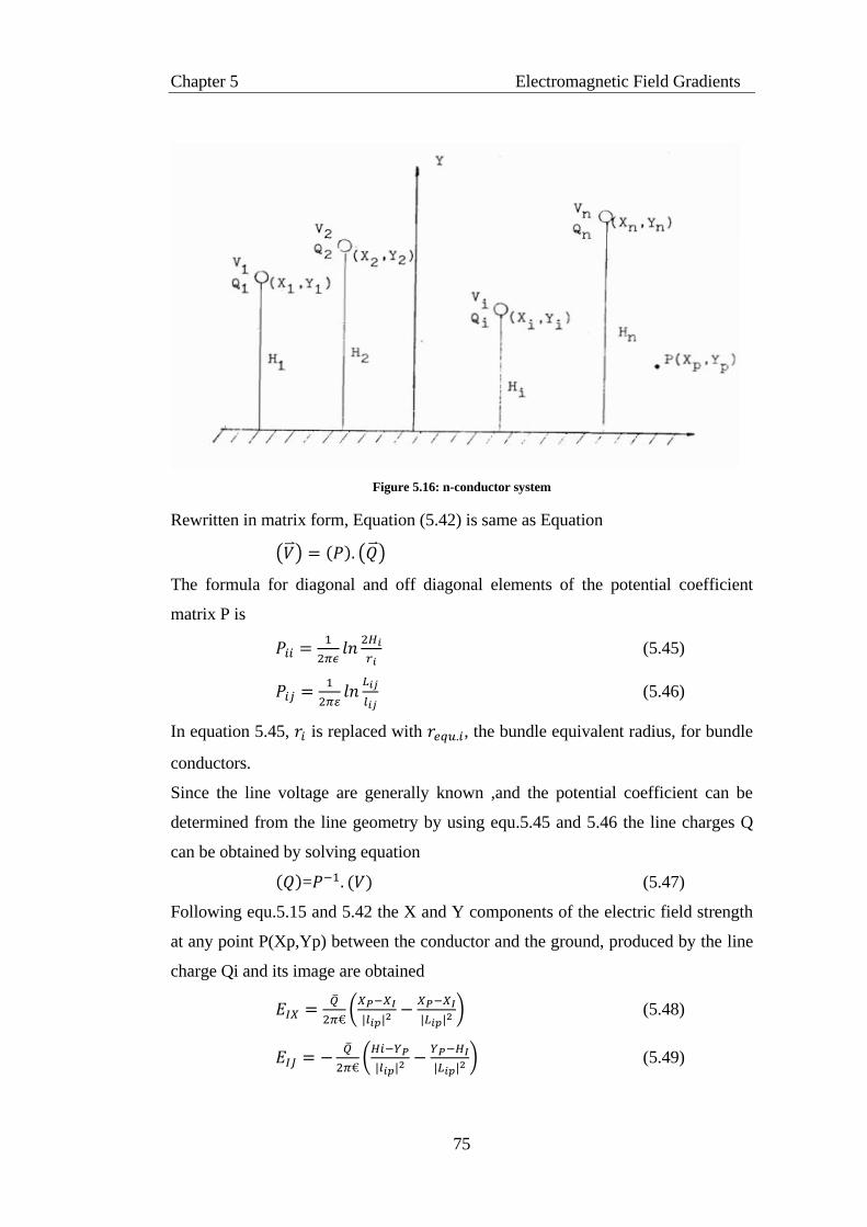
Chapter 5 Electromagnetic Field Gradients
75
Figure 5.16: n-conductor system
Rewritten in matrix form, Equation (5.42) is same as Equation
( ) ( )
The formula for diagonal and off diagonal elements of the potential coefficient
matrix P is
(5.45)
(5.46)
In equation 5.45, is replaced with , the bundle equivalent radius, for bundle
conductors.
Since the line voltage are generally known ,and the potential coefficient can be
determined from the line geometry by using equ.5.45 and 5.46 the line charges Q
can be obtained by solving equation
= (5.47)
Following equ.5.15 and 5.42 the X and Y components of the electric field strength
at any point P(Xp,Yp) between the conductor and the ground, produced by the line
charge Qi and its image are obtained
(
| |
| | ) (5.48)
(
| |
| | ) (5.49)

Chapter 5 Electromagnetic Field Gradients
76
Where are defined as in Equation 5.42.
For n conductor the resultant X and Y components of the electric field strength at P
are then obtained as
∑
∑ (
| |
| | )
(5.50)
∑
∑ (
| |
| | )
(5.51)
Finally, the resultent potential and electric field strength at P are
∑
(5.52)
√
∑ (
| |
| | )
(5.53)
Equation 5.53 is the required equation for calculation of electric field at a pont P.
5.3.4 Computer Program for calculation of Electric Fields
A program in MATLAB is written for the calculation of electric field. The input to
the program is the geometry of the tower, voltage magnitudes and the space (set of
points) in which the electric field is to be evaluated. The output of the program is
the value of electric field strengths, a plot of magnetic field strength versus distance
from transmission line and a complete profile of transmission line magnetic field
strength.
The program is divided into two functions. One of the functions is called by the
other function gives magnetic field strength against a single point input in the form
of x and y coordinates of the point. This function is called again and again for
501x501 points to evaluate magnetic field. The resultant matrix is then plotted
against the x and y arrays to form a magnetic field profile in the form of contours.
Tower geometry to the program is given by the six points, (x1, y1), (x2,
y2),….,(x6, y6). Tower geometry representing these points is given in Figure 5.5.
The computer Program is listed in Appendix B.
The overall electric field profile drawn by the program for three-phase double
circuit transmission line and six-phase single circuit line is given in Fig. 5.17
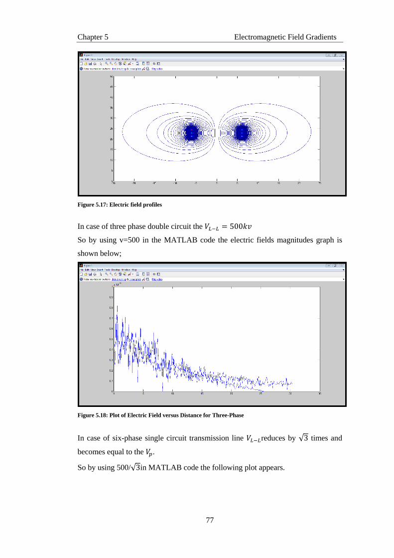
Chapter 5 Electromagnetic Field Gradients
77
Figure 5.17: Electric field profiles
In case of three phase double circuit the
So by using v=500 in the MATLAB code the electric fields magnitudes graph is
shown below;
Figure 5.18: Plot of Electric Field versus Distance for Three-Phase
In case of six-phase single circuit transmission line reduces by √ times and
becomes equal to the .
So by using 500/√ in MATLAB code the following plot appears.

Chapter 5 Electromagnetic Field Gradients
78
Figure 5.19: Plot of Electric Field versus Distance for Six-Phase
The geometry of the tower is same as it is given in Table 5.1 that has also been used
for the calculations of magnetic fields.
5.4 Corona
One of problem associated with HVDC and HVAC transmission lines is corona
power loss. Many attempts were made to solve ionized field using Charge
Simulation Method (CSM), Boundary Element Method, and Finite Element
Method.
But none of them has been taken in account the effect of the diffusion coefficient as
function of electric field and climate temperature and air density, etc.
The present method implements the potentials and electric field at conductor
surface as boundary conditions, however; in previous method deal only with the
potentials in conductor and ground plane and check the field on conductor surface
later.
The latest method for corona power loss calculation is FEM method that is used in
this paper, but some innovations, such as using new updating space charge densities
along electric field lines, instead of using flux-tube and writing continuity current
equation along it. In previous method programming calls for two loops to
convergence, one for convergence of potentials and another for convergence of
electric field at conductor surface. In this method only one loop is needed for
convergence of space charge density, this of course reduces the complexity if
computation and leads to reduction of the number of iterations, for updating space

Chapter 5 Electromagnetic Field Gradients
79
charge densities around the conductor, the rung-kutta integration method is used to
calculate charge densities along electric field lines, whereas previous method, using
flux-tubes along electric field lines [21].
5.4.1 Corona loss Calculations
The corona loss in a six-phase line can be obtained using the following empirical
formula, which is valid for three-phase lines also.
=
(f+25) √
(
kW/mile/conductor
where f = system frequency (Hz)
GMD = Geometric mean distance (cm)
= 15th root of all fifteen combinations of distance between the conductors of a six-
phase line
E = Maximum surface gradient (kV/cm)
𝛿 = Relative air density given by (a)
r = outside radius of conductor (cm)
= Corona initiation gradient (kV/cm) given by (b)
Now, 𝛿=
(a)
where b = atmospheric pressure (cm of mercury)
T = atmospheric temperature (°C)
The equation for = (
√ ) m (1+
√ ) (b)
where m = conductor surface factor, varying between 0.12 (wet) to 0.96 (dry).
Basic System Description Data:
SYSTEM VOLTAGE= 138.00 KV
NO. OF PHASES= 6
NO. OF CIRCULTS= 1
NO. OF SUBCONDUCTORS PER PHASE= I
TOTAL NO. OF GROUND WIRES= 2
EARTH RESISTIVITY= 100.00 OHM-METERS
FREQUENCY= 60.00 HZ
BASE POWER= 100.00 MVA
BASE VOLTAGE= 138.00 KV
Table 5.4: Line Configuration and Conductor Data
CONDUCTOR
DESIGNATION
Horizontal
Spacing
(FT)
Height
at
Tower
(FT)
Mid-Span
Clearance
(FT)
Radius
(FT)
GMR
(FT)
A - 68. 56. 0. 0.
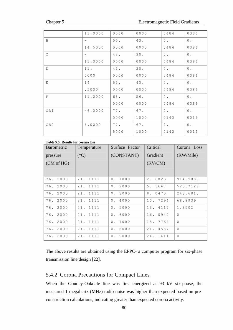
Chapter 5 Electromagnetic Field Gradients
80
11.0000 0000 0000 0484 0386
B -
14.5000
55.
0000
43.
0000
0.
0484
0.
0386
C -
11.0000
42.
0000
30.
0000
0.
0484
0.
0386
D 11.
0000
42.
0000
30.
0000
0.
0484
0.
0386
E 14
.5000
55.
0000
43.
0000
0.
0484
0.
0386
F 11.0000 68.
0000
56.
0000
0.
0484
0.
0386
GR1 -6.0000 77.
5000
67.
1000
0.
0143
0.
0019
GR2 6.0000 77.
5000
67.
1000
0.
0143
0.
0019
Table 5.5: Results for corona loss
Barometric
pressure
(CM of HG)
Temperature
(°C)
Surface Factor
(CONSTANT)
Critical
Gradient
(KV/CM)
Corona Loss
(KW/Mile)
76. 2000 21. 1111 0. 1000 2. 6823 914.9880
76. 2000 21. 1111 0. 2000 5. 3647 525.7129
76. 2000 21. 1111 0. 3000 8. 0470 243.6815
76. 2000 21. 1111 0. 4000 10. 7294 68.8939
76. 2000 21. 1111 0. 5000 13. 4117 1.3502
76. 2000 21. 1111 0. 6000 16. 0940 0
76. 2000 21. 1111 0. 7000 18. 7764 0
76. 2000 21. 1111 0. 8000 21. 4587 0
76. 2000 21. 1111 0. 9000 24. 1411 0
The above results are obtained using the EPPC- a computer program for six-phase
transmission line design [22].
5.4.2 Corona Precautions for Compact Lines
When the Goudey-Oakdale line was first energized at 93 kV six-phase, the
measured 1 megahertz (MHz) radio noise was higher than expected based on pre-
construction calculations, indicating greater than expected corona activity.
Chapter 5 Electromagnetic Field Gradients
81
Corona is a function of the electric field at the surface of the conductor and
hardware. Traditional laboratory tests for corona acceptability involve setting up a
specimen in a laboratory and energizing at some percentage above normal
operating voltage to check for corona inception. This method has worked well for
many years. However, it is not a complete test, because it is based on voltage, not
electric field. When conductors are more closely spaced than conventional design,
the electric field is greater for the same voltage. Thus, a piece of hardware may test
successfully in the laboratory, but may have excessive corona in actual operation. It
is frequently necessary to specify EHV-type corona free hardware for use on
compact 115 kV lines, because the electric field stress is actually more typical of a
345 kV line than a 115 kV line I ' The conductor shoes used on the original W-
shaped spacers installed in the compact section were of the standard design with
screw threads and nuts protruding from the bottom of the clamps, instead of the
corona-free variety. Also, fiber optic cable was initially wrapped on the bottom two
phases the entire length from Goudey to Oakdale. These were suspected of
contributing to the elevated radio noise levels.
An ultrasonic sound detector and VHF radio receiver were used to verify that the
spacer hardware and fiber optic cable were contributing to the elevated noise levels.
Measurements with these types of instruments taken in the compact section
revealed the following:
The ultrasonic detector revealed a raspy sound from the bottom two phases
similar to gap discharges. The bottom two phases clearly manifested
significantly greater electrical discharge of a different type than the other
four phases. These tests were performed from a bucket at approximately 45
feet above the ground. At this elevation unaided audible noise could be
heard in fair weather coming off the line. It was not possible to determine
which conductors were primarily contributing to the sound heard by ear.
Using the ultrasonic detector from the bucket between the tower and the
first in-span spacer, the noise was greater pointing at the spacer than at the
tower.
With the bucket alongside the spacer, the ultrasonic noise was greatest off
the bottom phases, with the maximum at the spacers. There was also a little
noise off the upper four phases which seemed to be coming from the ends of
Chapter 5 Electromagnetic Field Gradients
82
the conductor clamps of the spacers. No noise was detected from the ends of
the armor rods.
245 MHz noise peaked with a directional antenna pointed at the in-span
spacers from the bucket located between the tower and the first spacer. It
was not possible to distinguish the relative level of noise from the different
phases [23].
5.4.3 Results
Fig. 5.17 and fig. 5.18 clearly indicates that magnitude of electric field in case of
six-phase transmission is relatively smaller in magnitude. From this it can be
concluded that size of insulator required in six phase transmission towers will be
less as compared to the three-phase double circuit and size of tower will also be
compact as ground clearances and mid span clearances will be reduced. Eventually,
corona loss, radio interference, TV interference and formation of ozone due to
corona will also reduce as electric field strengths are diminished.
5.5 Summary
In this chapter electromagnetic field gradients of a transmission line have been
discussed. Computer programs are written in MATLAB and are used for plotting
the profiles of electric and magnetic fields in both three and six-phase transmission
lines. Finally, on the basis of electric field, corona loss in the transmission line is
determined. The results are in favor of six-phase transmission line. That is, six-
phase line has lower electromagnetic fields and corona loss.
Chapter 6 System Modifications and Cost Analysis
83
Chapter 6
System Modifications and Cost
Analysis
High phase order, the use of more than three phases for power transmission, has
been extensively studied in the last ten years. A number of papers and reports have
presented technical characteristics and benefits to be obtained by the use of more
than three phases. Increased power transfer over existing rights of way and reduced
electrical environmental impact are two of these benefits. However, for a
technology to be applied, it must be economically as well as technically beneficial.
After power transmission been analyzed by using the six phase system, it can be
concluded that, the six phase system is one an alternative to replace double three
phase circuit. Studies performed prove that transmission line with six phase system
has several advantages as high phase transmission line. Six phase transmission line
system get enhance the capability delivery as many 73% over with double circuit
three-phase system. Number phase increase will cause reduction gradient conductor
surface. For reduction of corona effect, audio noise, television and radio
interference and magnetic field giving good impact to the environmental. By
implement small development structure on the system use, it found affordable to
enhance the capability overhead line space on it system advantages.
Six-phase has already been shown to be an economic uprating tool for double
circuit lines. In this chapter, the modifications required in conversion of a three-
phase double circuit transmission line to a six-phase lines are discussed and
discussing the savings/expenses in terms of cost in all the equipment. Later a cost
analysis is performed in which a 500kV six-phase line is compared for relative
economics with a 500 kV three-phase double circuit design.
Chapter 6 System Modifications and Cost Analysis
84
6.1 System Modifications
In this section major modifications required in the power transmission system in
conversion of a three-phase double circuit transmission line to a six-phase
transmission line are discussed.
6.1.1 Six-Phase Conversion Transformers
As discussed in chapter 3, the most suitable way for the production of six-phase is
by using three-phase to six-phase conversion transformer. It can either be
constructed by using two three-phase transformers or six single phase transformers.
In practical conversion of three-phase double circuit transmission line to six-phase
line requires the installation of new six-phase transformers. [18] However
depending upon the life, the existing transformers can be used in forming a
transformer conversion bank. At high voltage levels usually three-single phase
transformers are used to form the three-phase transformer, so in six-phase
conversion, three more transformers need to be installed. In case a three phase
transformer is installed, then another three-phase need to be purchased. So in using
the existing transformers in forming the six-phase conversion bank there is saving
of three single phases (or a three phase) transformers.
Further, the installation of new three-phase transformers is justifiable. As the power
transmission capacity is being enhanced, the transformer required must be of higher
rating to meet the enhanced power flow. So, the transformers of higher rating are
always needed even if the method of power transfer capability enhancement is
other than six-phase transmission.
6.1.2 Six Phase Positioning
Design of Substation modifications for six phase transmission requires careful
attention to detail regarding the phasing arrangement, since it will have greater than
normal impact on the physical arrangements. Since the six-phase configuration is
mostly achieved through the use of two three-phase transformers using Delta-Wye
and Delta-Inverted Wye configurations, the phasing arrangement of the six phase
system (1-2-3-4-5-6) can be visualized as being built with subsets of two three
phase systems, one set comprised of phase 1-3-5 and the second comprised of
phase 2-4-6. In vector the two sets are 180o out of phase, but when electrically
configured into a six phase system, it will result in vector displacement of 60
degrees between adjacent phases.[24] Proper phasing is exercised to ensure that
each three phase conductor subset of the six-phase system is connected to the
Chapter 6 System Modifications and Cost Analysis
85
appropriate transformer terminals at each end of the line. In addition, adequate
clearances are maintained during phase transposition of conductors at the
secondaries of transformers since the voltage difference between adjacent phases
conductors could be 1 pu or 1.73 pu or 2 pu as discussed in chapter 2. This was a
critical issue for the conductor connections between the transformer take-off
structure and first tower of transmission line. So it requires space and structures for
the said purpose at the substation with extension is the ground grid that ultimately
appears in the form of increase in cost.
Phase transposition from the transformers to the first transmission tower of the six
phase line could have been achieved in one of two ways:
1. Provision of phase transposition buses on top of the takeoff structure.
2. Phase transposition at the transmission tower itself utilizing additional
insulator strings and cross over jumpers to achieve the designated vector
configuration.
6.1.3 Six-phase Bays
Apart from the need for the positioning structures transformer and switching bays
are required for six-phase at high voltages. [25] These bays provide housing for the
six-phase transformers and circuit breakers respectively. These structures are
similar to that of the phase positioning structures and also have a similar impact on
cost.
6.1.4 Protection
The concept of protection in six-phase is entirely different from that of three-phase
transmission system. Faults in six-phase transmission lines are much more
complicated than that of three-phase transmission lines, and the types of short-
circuit faults are as many as 120 in species that is only 11 in three-phase system.
Further, the number of significant faults in six-phase is 23 whereas in three-phase
are only 5.
Currently, foreign scholars have conducted some research on the six-phase
transmission system faults. Reference [26] accurately expressed the symmetrical
arrangement electromagnetic coupling sequence and derived the fault current
expression based on the analysis of various fault types of six-phase system.
Seeking the complexity of protection in six-phase transmission system it must be
given attention. So, it requires the installation of intelligent and sophisticated
protection equipment for current differential line protection and appropriate
Chapter 6 System Modifications and Cost Analysis
86
transformer protection. Also requires specially modified auto reclosing and
synchronizing relays, breaker failure protection for each line breaker, pole
disagreement protection, and metering. This is a costing factor in six-phase system.
6.1.5 Transmission line Modifications
In uprating three-phase double circuit transmission line to six-phase transmission
line, 73% power enhancement is achieved. That is the power transferring is under
the same structures. It is proved in chapter 4, that even after converting a three-
phase double circuit transmission line to six-phase single circuit transmission line,
there is no change in the line currents. The currents in each phase have the same
magnitudes as before in three-phase double circuit transmission line conductors.
So, there is no need of re-conductoring, which is the major cost saving in six-phase
transmission system.
6.1.6 Insulation Requirements
We know that in six-phase transmission line, the phase to ground voltage increases
to line to line voltage. Thus the system voltage is again the same as in three-phase
double circuit transmission line. Calculations done in chapter 2 showed that the
maximum potential that exists between any two phases in a six-phase transmission
system is not more than 2 p.u. Research shows that if proper [27] positioning of all
the six-phases is done on an existing three-phase double circuit transmission tower,
there is no need to provide extra insulators on transmission line. This is again
saving in terms of cost.
If the load is not increased in conversion from three-phase double circuit
transmission line to six-phase transmission line, that is the line to line voltage is
reduced to phase to ground voltages, the insulation requirements considerably
reduce due to reduction in the system voltage.
6.1.7 Tower Structures
Transmission towers are priced according to their weight. Thus, tower weight is a
primary parameter in the economic analysis. Each tower was fully designed and all
members properly sized. Three-phase double circuit transmission line to six-phase
transmission line reduces the requirements of supporting structures. [28]
Transmission towers are designed to carry the load of the conductors hanged with
the insulators. As in three-phase to six phase conversion, there is no need to
reconductoring nor are the excessive insulators required. So, as a result the steel
structures required to carry the conductor and insulators reduced. Further, due to

Chapter 6 System Modifications and Cost Analysis
87
lesser electric field in six-phase power transmission, the less spacing requirement
between the six-phase conductors results in the smaller arms of transmission tower.
So, in constructing a new transmission six-phase line in comparison to three-phase
double circuit line has a lot of saving in terms of capital required.
6.1.8 Right of Ways
The required width of Right of Way is based on electrical system parameters. As
discussed in previous chapters that electric and magnetic field gradients of a three-
phase to six-phase converted transmission line are within the limits governed by the
health authorities. So, the Right of Way span required for six-phase power
transmission line is not greater than that of three-phase transmission line. Further,
reduced electromagnetic field gradients results in compact structures allow a lot of
saving in constructing a new six-phase transmission line.
While there is a minimum required width for any transmission line, it would not be
correct to assume that all utilities would use the minimum. Also, the cost of ROW
varies widely for different locations and areas, making it difficult to assign a
meaningful dollar-per-acre ROW cost. For these reasons, cost differences for the
candidate lines studied are presented only as a single illustration, and are not
included in the general case. The ROW requirements of EHV high phase order
lines are less than those of three-phase double circuit transmission lines, and can
result in a significant cost advantage [29].
6.2 Cost Analysis
In this section we introduce a transmission line carrying a specific amount of load.
Which is to be uprated to carry some extra load, the options considered are the six-
phase conversion and other cheapest possible i.e. the re-conductoring of existing
line with a conductor having greater thermal capacity. For this Economic Analysis,
it is assumed that there is a double circuit 500 kV line between two substations
which requires an increase in power flow capability. The existing line was assumed
to be constructed with 795 kcmil ACSR (Drake) conductors, with combined
capability for the two circuits of 1400 MVA. The existing substation was assumed
to be a 500 kV breaker and a half arrangement with 1200 ampere rated equipment.
The system was assumed to require uprating to carry an additional 900 MVA.
One option to obtain a rating increase would be to reconductor the line with 795
kcmil ACSR conductor by bundling with the existing conductor. For the assumed
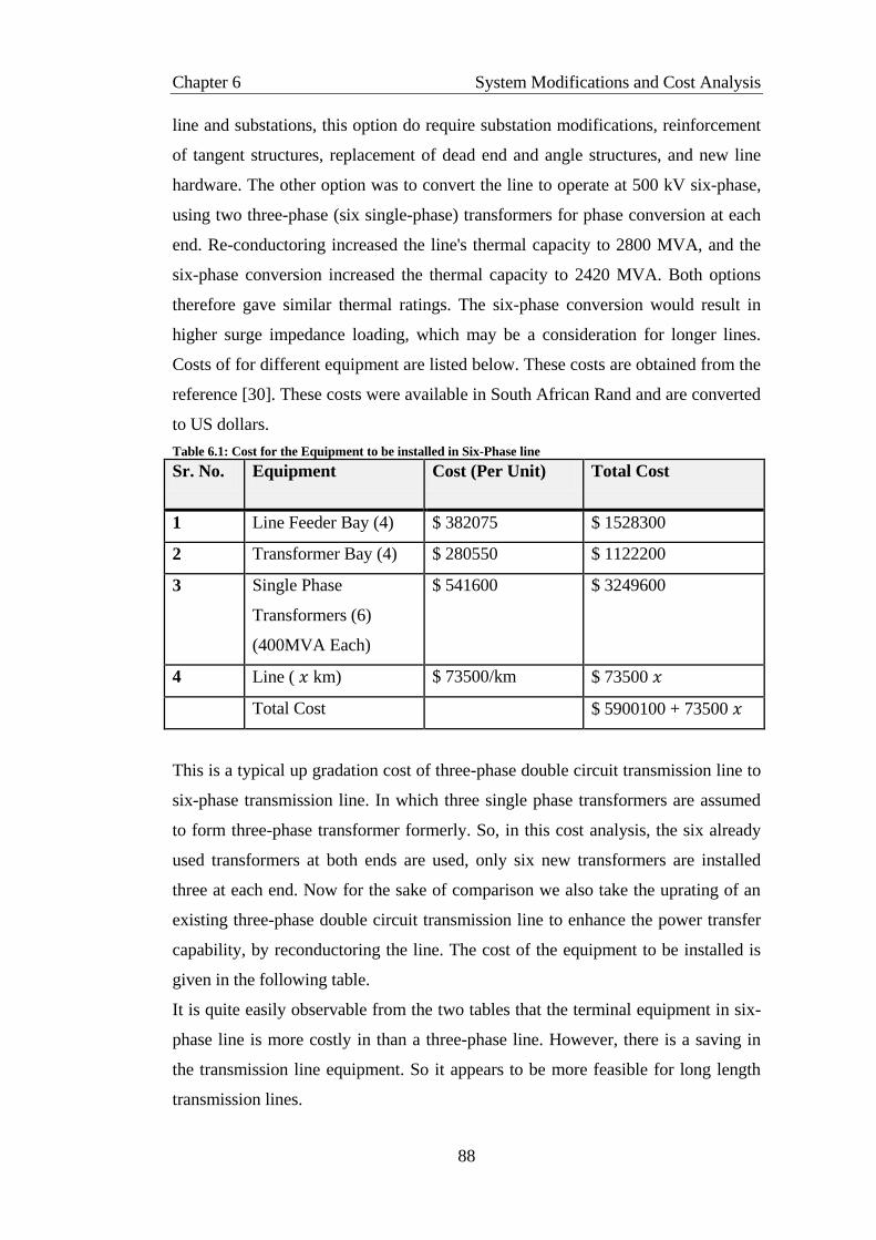
Chapter 6 System Modifications and Cost Analysis
88
line and substations, this option do require substation modifications, reinforcement
of tangent structures, replacement of dead end and angle structures, and new line
hardware. The other option was to convert the line to operate at 500 kV six-phase,
using two three-phase (six single-phase) transformers for phase conversion at each
end. Re-conductoring increased the line's thermal capacity to 2800 MVA, and the
six-phase conversion increased the thermal capacity to 2420 MVA. Both options
therefore gave similar thermal ratings. The six-phase conversion would result in
higher surge impedance loading, which may be a consideration for longer lines.
Costs of for different equipment are listed below. These costs are obtained from the
reference [30]. These costs were available in South African Rand and are converted
to US dollars.
Table 6.1: Cost for the Equipment to be installed in Six-Phase line
Sr. No. Equipment Cost (Per Unit) Total Cost
1 Line Feeder Bay (4) $ 382075 $ 1528300
2 Transformer Bay (4) $ 280550 $ 1122200
3 Single Phase
Transformers (6)
(400MVA Each)
$ 541600 $ 3249600
4 Line ( km) $ 73500/km $ 73500
Total Cost $ 5900100 + 73500
This is a typical up gradation cost of three-phase double circuit transmission line to
six-phase transmission line. In which three single phase transformers are assumed
to form three-phase transformer formerly. So, in this cost analysis, the six already
used transformers at both ends are used, only six new transformers are installed
three at each end. Now for the sake of comparison we also take the uprating of an
existing three-phase double circuit transmission line to enhance the power transfer
capability, by reconductoring the line. The cost of the equipment to be installed is
given in the following table.
It is quite easily observable from the two tables that the terminal equipment in six-
phase line is more costly in than a three-phase line. However, there is a saving in
the transmission line equipment. So it appears to be more feasible for long length
transmission lines.

Chapter 6 System Modifications and Cost Analysis
89
Table 6.2: Cost of the equipment for uprating of three-phase double circuit line.
Sr.
No.
Equipment Cost (Per Unit) Total Cost
1 Line Feeder Bay (2) $ 520150 $ 1040300
2 Transformer Bay (2) $ 376584 $ 735168
3 Three- Phase
Transformers (2)
(400MVA Each)
$ 1992700 $ 3985400
4 Line ( km) $ 90780/km $ 90780
Total Cost $ 5760868 + 90780
At the end of the two tables above, the total cost equation for six-phase and three-
phase double circuit transmission line is given. These equations are equated to give
the breakeven distance, i.e. the length of line where the cost of six-phase line is
equal to that of three-phase double circuit transmission line. This is the minimum
length for which the six-phase line is beneficial.
Figure 6.1: Plot of Total Line Costs for Six-phase and three-phase double circuit lines.
Figure shows that breakeven distance occurs at 9km. So, for this particular line the
six-phase configuration of transmission line capability is enhanced only if the line
has a length greater than 9km.

Chapter 6 System Modifications and Cost Analysis
90
6.3 Summary
In this chapter various system modifications are discussed that are needed in
uprating an existing three-phase double circuit transmission line. Saving and costs
in substation equipment, protection equipment and lines are discussed. At the end a
cost comparison of six-phase transmission line made with a three-phase
transmission line and it was found that a 500kV transmission line has a benefit is
uprating to six-phase line in terms of cost if the line length is more than 6 km.
Chapter 7 Conclusions and Future Recommendations
91
Chapter 7
Conclusions and Future
Recommendations
This thesis provides a base for the six-phase transmission system and it explains
some basic rules about the six phase power, where the complexity in different
voltages in six-phase system is discussed in detail. Moreover, methods have been
established for the production of six-phase power and analysis has been performed
on the three-phase to six-phase conversion transformers. After establishing basics,
six-phase transmission line is modeled in MATLAB Simulink and
SimPowerSystems. Where analyses have been performed for the power
enhancement capability, checked and verified the voltage and phasor relationships
developed earlier. The voltage drop along the length of a six-phase transmission
line is also discussed as a comparison with three-phase double circuit transmission
line. Later on, Electric and Magnetic Field Gradients in a transmission line are
discussed and analyzed. A comparison of three-phase double circuit transmission
line with six-phase transmission line is done.
In this chapter the results of all the analysis performed are summarized and
discussed. The conclusions are made and limitations of this study are discussed and
finally recommendations are made for further study in this field.
7.1 Results and Conclusions
Following results and conclusions can be made from the calculations, analyses and
simulation performed in this project.
1. In three phase to six-phase conversion, line to line voltage can be made
equal to phase to ground voltage or alternatively phase to ground voltage
Chapter 7 Conclusions and Future Recommendations
92
can be increased to line to line voltage. This voltage level transform
depends upon conversion transformers. Four different types of voltages
exist in Six-phase system those are phase-to-ground voltage, between
adjacent phases, between phases separated by one intermediate phase and
between opposite phases.
2. Out of five common transformer configurations, Double Delta and Y-Y &
Y-Inverted Y configuration decrease line to line voltage to make equal to
phase to neutral voltage, whereas in ∆-Y & ∆-Inverted Y, Diametrical and
Double Y configuration phase to neutral voltage is increased to line to line
voltage.
3. Six-phase transmission line parameters such as SIL, Line Loadibility and
stability can be computed by using the same techniques as used for three-
phase transmission line.
4. Six-phase transmission have several advantages over the three-phase
transmission that include higher power transfer capability, increased
utilization of right of way, increased power density, smaller line structures,
less insulation requirements, better stability margins, lower corona and field
effects and better lighting performance.
5. Simulation results show that power transfer capability is enhanced in six-
phase transmission in comparison to three-phase by 73% with the same line
current and same line-to line voltage.
6. Voltage Drops across the six-phase transmission line are greater than three-
phase transmission line and has poor voltage regulation and poor voltage
stability with increase in distance and power flow respectively. This is a
drawback of six-phase power transmission line.
7. Magnetic field plots of six-phase line show that under the same loads of as
of a three-phase double circuit transmission line, magnetic fields are less
than three-phase double circuit transmission line. But with 73% power
enhancement magnetic fields are a bit increased but are far less than the
limits set by the Environment and Health Authorities.
8. Electric field plots of six-phase transmission line are also less than those of
three-phase double circuit transmission line, that gives a room for the
compaction of transmission structures and also provide cost saving for
insulators.
Chapter 7 Conclusions and Future Recommendations
93
9. Corona Loss in Six-phase is also less due to low electric field profiles.
10. Seeking these benefits, a three-phase double circuit transmission line can be
converted to six-phase line on the existing transmission structures, only
modifications required are to be made at terminals.
11. Cost comparison of power capability enhancement of three-phase double
circuit transmission line by reconductoring to that converting to six-phase
show that six-phase is more economical if line length is more than 9
kilometers.
So it is concluded that six-phase transmission is a solution to the limitations offered
in three-phase power transfer capability enhancement due to unavailability of right
of ways, electric and magnetic fields constraints due to health hazards and provides
a cost effective solution of upgrading existing transmission lines to six-phase lines.
So 73% more power can be transferred by the existing transmission lines without
any modifications in transmission lines but the modifications are made at sending
and receiving end of transmission line in the form of conversion and inversion
transformer. For the same load, corona loss, radio interference, TV interference etc.
are reduced due to which clearances required from the tower or in other sense size
of tower is reduced to much extent. All these results have been verified with the
help of simulations performed on Simulink® and MATLAB™ programs.
7.2 Project Limitations and Future Recommendations
Following are the project limitations and future recommendations for six phase
power transmission system:
1. In this project, the simulation of six-phase power transmission line is
performed on MATLAB Simulink and SimPowerSystems. The accuracy of
MATLAB is limited. Professional power software should be used in future
for more accurate results like PSCAD, PSSE etc.
2. For the calculations of magnetic and electric fields, dedicated tools are
developed in MATLAB by our own that provide the two dimensional
profile of the fields. In future research can be performed on the professional
tools that give three dimensional plots of field gradients with more accurate
results such as EMF WORKSTATION.
3. In this project transformer connections and their primary and secondary
voltage levels are analyzed for six-phase conversion banks. A more detailed

Chapter 7 Conclusions and Future Recommendations
94
studied is needed for six-phase transformers and its characteristic under six-
phase operation.
4. Research should be done at practical level by the Transmission companies
by implementing hardware on a long length of transmission line e.g. NTDC
should consider six-phase transmission lines for future transmission line
construction.

References
95
References
[1] A.S. Pandya, R.B Kelkar, „‟An Innovative Transmission Alternate-High
phase order Transmission system” A Paradigm to Enhance Power System
Capability Proc. National Conference on recent trends in power system at
S.N. Institute of Science and Technology, Hyderabad, Nov-2005.
[2] M. W. Mustafa, M. R. Ahmad and H. Shareef, “Fault analysis on double
three-phase to six-phase converted transmission line”, IEEE power engg.
Conference IPBC 2005.
[3] M.A. Golkar,Reza Shariatinasab, Mohsen Akbari “Voltage Stability
Analysis in Conversion of Double Three phase to Six phase Transmission”
Kuala Lumpur, Malaysia Nov 2010.
[4] Glover, J. D., and Sarma, M. S., “Power System Analysis and Design” USA:
Brooks/Cole Thomson Learning Companies. 3rd Ed. 2002.
[5] Fostescue, C. L., “Method of Symmetrical Coordinates Applied to the
Solution of Poly-phase Networks”. AIEE Transactions.1918.Vol. 37. 1027
1140, Oct 2004.
[6] Clark, E., “Circuit Analysis of AC Power System” John Wiley & Sons, Vol.
I. Inc.New York. Edition 2009.
[7] Ammar A. Hajjar, M.M. Mansour, H.E.A.Talaat, S.O.Faried, “Distance
protection for six-phase transmission lines based on fault induced high
frequency transients and wavelets”, Proceedings of the 2002 IEEE Canadian
Conference on Electrical & Computer Engineering, 2002.
[8] Billinton, R., Faried, S. O., and Firuzabad, M. F., “Composite System
Reliability Evaluation Incorporating a Six-Phase Transmission Line”. IEE
Proc.-Generation Transmission Distribution. Vol. 150. 413-419. 2003.
[9] James. R. S and Thomas L. H, “138kV 12-Phase as an Alternative to 345kV
3-Phase”. IEEE Transaction on Power Delivery, Vol.13, No.4, October
1998.
[10] Hussein Ahmad and Jambak, M. I., “Advanced Laboratory Scale Model of
High Phase Conversion Power Transmission Line” 2nd IEEE International
References
96
Conference on Power and Energy (PECon 08), Johor Baharu, Malaysia,
December 1-3, 2008.
[11] Venkata, S. S., “Reliability and Economics Analysis of Higher Phase Order
Electric Transmission System”. Final Report on Grant No. 74 ENGR 10400,
1997.
[12] Dorazio, T. F., “High Phase Order Transmission”. IEEE No. 90TH0313-7.
NYSEG. Binghamton, New York, 1990.
[13] Stewart, J. R., Oppel, L.J., Thomann, G. C., Dorazio, T. F., and Brown, M.
T., “Insulation Coordination, Environmental and System Analysis of
Existing Double Circuit Line Reconfigured to Six-Phase Operation” IEEE
Transaction on Power Delivery. Vol. 7, No. 3. 1628-1633, 1992.
[14] W. L. Tucker, NSWC Caderock Division, “Analysis and Simulation of a
Six-Phase Generator/Rectifier System” IEEE power engg. Conference IPBC
2005.
[15] Zimmerman, R. D., Carlos, E. M., and Gan, D. MATPOWER- A
MATLAB™ Power System Simulation Package. Power Systems
Engineering Research Center (PSERC), School of Electrical Engineering,
Cornell University, Ithaca, NY. User‟s Manual, Version 3.0b1. 2004.
[16] Mustafa, M. W., and Ahmad, M. R., “Transient Stability Analysis of Power
System with Six-Phase Converted Transmission Line”. PECon 2006, First
International Power and Energy Conference, Putra Jaya, Malaysia. Vol.1.
262-266. 2006.
[17] http://www.mathworks.com/
[18] Siti Amely Binti Jumaat, Prof Madya Dr. Mohd, “Analysis Of Six-Phase
System For Transmission Line” The 2nd International Power Engineering
and Optimization Conference (PEOCO2008), Shah Alam, Selangor,
MALAYSIA. 4-5 June 2008.
[19] S.Y. king, “Improved solution for the field near bundle conductors”, Proc.
IEE (London), Vol. 110, No. 6, pp. 1044-1050, 2006.
[20] Jong Sen Hsu, “Transmission Line Conductor Surface Voltage Gradient and
Magnetic Flux Denrity Computations”, M. Sc. Thesis, the Ohio State
University, Columbus, 1980.
[21] M. Mohammadi, R.Ebrahimi, “Corona Losses Calculation in HVAC
Transmission Lines Using FEM and Comparison with HVDC Corona
References
97
Losses”, Australian Journal of Basic and Applied Sciences, 5(5): 833-843,
ISSN 1991-8178, 2011.
[22] S.S. Venkata, W.C. Guyker, J. Kondragunta, “EPPC - A computer program
for six-phase transmission line design” IEEE Transactions on Power
Apparatus and Systems, Vol. PAS-101, No. 7 July 1982.
[23] J.R. Stewart, L.J. Oppel, R.J. Richeda, “Corona and Field Effects Experience
on an Operating Utility Six-Phase Transmission Line” IEEE Transactions on
Power Delivery, Vol. 13, No. 4, October 1998.
[24] M.T. Brown, R.V. Rebbapragada “Design Modification and Layout of
Utility Substations for Six Phase Transmission” IEEE Transactions on Power
Delivery, Vol. 8, No. 1, January 2003.
[25] Kundur. P., “Power System Stability and Control”. McGraw-Hill, Inc. New
York.2001.
[26] Badawy, E. H., El-Sherbiny, M. K., and Ibrahim, A. A., “A Method of
Analyzing Unsymmetrical Faults on Six-Phase Power Systems” IEEE
Transaction on Power Delivery. Vol. 6, No.3. 1139-1145, 1992.
[27] Stewart, J. R., and Wilson, D. D., “High Phase Order Transmission – A
Feasibility Analysis: Part II – Overvoltages and Insulation Requirements”
IEEE Transaction on Power Apparatus and System. Vol. PAS-97, No. 6.
2308-2317. 2007.
[28] I. S. Grant, J. R. Stewart, “Mechanical And Electrical Characteristics of
EHV High Phase Order Overhead Transmission” IEEE Transaction on
Power Apparatus and Systems, Vol. PAS-103, No. 11, November 1984.
[29] J. R. Stewart, E. Kallaur, “Economics Of EHV High Phase Order
Transmission” Transaction on Power Apparatus and Systems, Vol. PAS-103,
No. 11, November 2004.
[30] Jacob Bortnik, “Transmission Line Compaction using High Phase Order
Transmission” University of Witwatersrand, Johannesburg, M.Sc Student
Thesis, Juhannesburg, 1998.

Appendix A MATLAB Function for magnetic field calculation
98
Appendix A
MATLAB function for
magnetic field calculations
A.1 Function for magnetic fields
xp=0;
yp=0;
x1=-6.1; x2=-6.1; x3=-6.1; x4=6.1; x5=6.1; x6=6.1;
y1=24.38; y2=22.86; y3=21.34; y6=24.38; y5=22.86; y4=21.34;
a=1/2; b=sqrt(3)/2; I=1000;
R1= sqrt(power((xp-x1),2)+ power((y1-yp), 2) ); R2= sqrt(power((xp-x2),2)+ power((y2-yp), 2) ); R3= sqrt(power((xp-x3),2)+ power((y3-yp), 2) ); R4= sqrt(power((xp-x4),2)+ power((y4-yp), 2) ); R5= sqrt(power((xp-x5),2)+ power((y5-yp), 2) ); R6= sqrt(power((xp-x6),2)+ power((y6-yp), 2) );
Ir1 = I*1; Ii1=0*I; Ir2 = I*a; Ii2=-b*I; Ir3 = -a*I; Ii3=-b*I; Ir4 = -1*I; Ii4=0*I; Ir5 = -a*I; Ii5=b*I; Ir6 = a*I; Ii6=b*I;

Appendix A MATLAB Function for magnetic field calculation
99
Hpxr1 = Ir1*(y1-yp)/(2*pi*power(R1, 2)); Hpxr2 = Ir2*(y2-yp)/(2*pi*power(R2, 2)); Hpxr3 = Ir3*(y3-yp)/(2*pi*power(R3, 2)); Hpxr4 = Ir4*(y4-yp)/(2*pi*power(R4, 2)); Hpxr5 = Ir5*(y5-yp)/(2*pi*power(R5, 2)); Hpxr6 = Ir6*(y6-yp)/(2*pi*power(R6, 2));
Hpxr = Hpxr1 + Hpxr2 + Hpxr3 + Hpxr4 + Hpxr5 + Hpxr6 ;
Hpxi1 = Ii1*(y1-yp)/(2*pi*power(R1, 2)); Hpxi2 = Ii2*(y2-yp)/(2*pi*power(R2, 2)); Hpxi3 = Ii3*(y3-yp)/(2*pi*power(R3, 2)); Hpxi4 = Ii4*(y4-yp)/(2*pi*power(R4, 2)); Hpxi5 = Ii5*(y5-yp)/(2*pi*power(R5, 2)); Hpxi6 = Ii6*(y6-yp)/(2*pi*power(R6, 2));
Hpxi = Hpxi1 + Hpxi2 + Hpxi3 + Hpxi4 + Hpxi5 + Hpxi6 ;
Hpyr1 = Ir1*(xp-x1)/(2*pi*power(R1, 2)); Hpyr2 = Ir2*(xp-x2)/(2*pi*power(R2, 2)); Hpyr3 = Ir3*(xp-x3)/(2*pi*power(R3, 2)); Hpyr4 = Ir4*(xp-x4)/(2*pi*power(R4, 2)); Hpyr5 = Ir5*(xp-x5)/(2*pi*power(R5, 2)); Hpyr6 = Ir6*(xp-x6)/(2*pi*power(R6, 2));
Hpyr = Hpyr1 + Hpyr2 + Hpyr3 + Hpyr4 + Hpyr5 + Hpyr6;
Hpyi1 = Ii1*(xp-x1)/(2*pi*power(R1, 2)); Hpyi2 = Ii2*(xp-x2)/(2*pi*power(R2, 2)); Hpyi3 = Ii3*(xp-x3)/(2*pi*power(R3, 2)); Hpyi4 = Ii4*(xp-x4)/(2*pi*power(R4, 2)); Hpyi5 = Ii5*(xp-x5)/(2*pi*power(R5, 2)); Hpyi6 = Ii6*(xp-x6)/(2*pi*power(R6, 2));
Hpyi = Hpyi1 + Hpyi2 + Hpyi3 + Hpyi4 + Hpyi5 + Hpyi6;
Hpx = Hpxr + j*Hpxi Hpy = Hpxr + j*Hpyi
Hx=[Hpx Hpy]
A.2 Function for Plotting Profiles
x=-25:0.1:25; y=0:0.1:50; H=zeros(501,501); for d=1:501 for e=1:501 H(d,e)= magnet14 (x(1,e), y(1,d)); end end H figure contour(x,y,H,2000);
1. Function for Plotting Characteristics y=0:0.1:50 x=(y-22.86*(ones(size(y))))/(-2);

Appendix A MATLAB Function for magnetic field calculation
100
R=zeros(size(x)) H=zeros(501,1) for d=1:501 H(d,1) = abs(magnet14 (x(1,d), y(1,d))); R(1,d)=sqrt(power(x(1,d),2)+ power((22.86-y(1,d)), 2)
);
end H
plot(R,H);
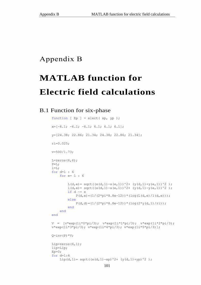
Appendix B MATLAB function for electric field calculations
101
Appendix B
MATLAB function for
Electric field calculations
B.1 Function for six-phase function [ Ep ] = elect( xp, yp );
x=[-6.1; -6.1; -6.1; 6.1; 6.1; 6.1];
y=[24.38; 22.86; 21.34; 24.38; 22.86; 21.34];
ri=0.025;
v=500/1.73;
L=zeros(6,6); P=L; l=L; for d=1 : 6 for e= 1 : 6
L(d,e)= sqrt((x(d,1)-x(e,1))^2+ (y(d,1)+y(e,1))^2 ); l(d,e)= sqrt((x(d,1)-x(e,1))^2+ (y(d,1)-y(e,1))^2 ); if d ~= e P(d,e)=(1/(2*pi*8.8e-12))*(log(L(d,e)/l(d,e))); else P(d,d)=(1/(2*pi*8.8e-12))*(log(2*y(d,1)/ri)); end end end
V = [v*exp(1i*0*pi/3); v*exp(1i*1*pi/3); v*exp(1i*2*pi/3);
v*exp(1i*3*pi/3); v*exp(1i*4*pi/3); v*exp(1i*5*pi/3)];
Q=inv(P)*V;
Lip=zeros(6,1); lip=Lip; Ep=0; for d=1:6 Lip(d,1)= sqrt((x(d,1)-xp)^2+ (y(d,1)+yp)^2 );

Appendix B MATLAB function for electric field calculations
102
lip(d,1)= sqrt((x(d,1)-xp)^2+ (y(d,1)-yp)^2 ); Ep = Ep + (-1/(2*pi*8.8e-
12))*Q(d,1)*((lip(d,1))/((abs(lip(d,1)))^2) -
(Lip(d,1)/((abs(Lip(d,1)))^2))); end Ep=abs(Ep); End
B.2 Function for three-phase
function [ Ep ] = elect( xp, yp );
x=[-6.1; -6.1; -6.1; 6.1; 6.1; 6.1];
y=[24.38; 22.86; 21.34; 24.38; 22.86; 21.34];
ri=0.025;
v=500;
L=zeros(6,6); P=L; l=L; for d=1 : 6 for e= 1 : 6
L(d,e)= sqrt((x(d,1)-x(e,1))^2+ (y(d,1)+y(e,1))^2 ); l(d,e)= sqrt((x(d,1)-x(e,1))^2+ (y(d,1)-y(e,1))^2 ); if d ~= e P(d,e)=(1/(2*pi*8.8e-12))*(log(L(d,e)/l(d,e))); else P(d,d)=(1/(2*pi*8.8e-12))*(log(2*y(d,1)/ri)); end end end
V = [v*exp(1i*0*pi/3); v*exp(1i*1*pi/3); v*exp(1i*2*pi/3);
v*exp(1i*3*pi/3); v*exp(1i*4*pi/3); v*exp(1i*5*pi/3)];
Q=inv(P)*V;
Lip=zeros(6,1); lip=Lip; Ep=0; for d=1:6 Lip(d,1)= sqrt((x(d,1)-xp)^2+ (y(d,1)+yp)^2 ); lip(d,1)= sqrt((x(d,1)-xp)^2+ (y(d,1)-yp)^2 ); Ep = Ep + (-1/(2*pi*8.8e-
12))*Q(d,1)*((lip(d,1))/((abs(lip(d,1)))^2) -
(Lip(d,1)/((abs(Lip(d,1)))^2))); end Ep=abs(Ep); end
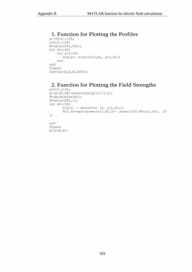
Appendix B MATLAB function for electric field calculations
103
1. Function for Plotting the Profiles x=-25:0.1:25; y=0:0.1:50; H=zeros(501,501); for d=1:501 for e=1:501 H(d,e)= elect(x(1,e), y(1,d)); end end figure contour(x,y,H,2000);
2. Function for Plotting the Field Strengths y=0:0.1:50; x=(y-22.86*(ones(size(y))))/(-2); R=zeros(size(x)); H=zeros(501,1); for d=1:501 H(d,1) = abs(elect (0, y(1,d))); R(1,d)=sqrt(power(x(1,d),2)+ power((22.86-y(1,d)), 2)
);
end figure plot(R,H);
Related Documents