SISMID Spatial Statistics in Epidemiology and Public Health 2015 R Notes: Cluster Detection and Clustering for Count Data Jon Wakefield Departments of Statistics and Biostatistics, University of Washington 2015-07-21

Welcome message from author
This document is posted to help you gain knowledge. Please leave a comment to let me know what you think about it! Share it to your friends and learn new things together.
Transcript

SISMID Spatial Statistics in Epidemiology andPublic Health
2015 R Notes: Cluster Detection and Clusteringfor Count Data
Jon WakefieldDepartments of Statistics and Biostatistics, University of
Washington
2015-07-21

North Carolina SIDS Data
The nc.sids data frame has 100 rows and 21 columns and can befound in the spdep library.
It contains data given in Cressie (1991, pp. 386-9), Cressie andRead (1985) and Cressie and Chan (1989) on sudden infant deathsin North Carolina for 1974–78 and 1979–84.
The data set also contains the neighbour list given by Cressie andChan (1989) omitting self-neighbours (ncCC89.nb), and theneighbour list given by Cressie and Read (1985) for contiguities(ncCR85.nb).
Data is available on the numbers of cases and on the number ofbirths, both dichotomized by a binary indicator of race.
The data are ordered by county ID number, not alphabetically as inthe source tables.

North Carolina SIDS DataThe code below plots the county boundaries along with theobserved SMRs.
The expected numbers are based on internal standardization with asingle stratum.
library(maptools)library(spdep)nc.sids <- readShapePoly(system.file("etc/shapes/sids.shp",
package = "spdep")[1], ID = "FIPSNO",proj4string = CRS("+proj=longlat +ellps=clrk66"))
nc.sids2 <- nc.sids # Create a copy, to add toY <- nc.sids$SID74E <- nc.sids$BIR74 * sum(Y)/sum(nc.sids$BIR74)nc.sids2$SMR74 <- Y/Enc.sids2$EXP74 <- Ebrks <- seq(0, 5, 1)rm(nc.sids) # We load another version of this later, so tidy up here

SMR PlotWe map the SMRs, and see a number of counties with high relativerisks.
spplot(nc.sids2, "SMR74", at = brks,col.regions = grey.colors(5, start = 0.9,
end = 0.1))
0
1
2
3
4
5
Figure 1: Map of SMRs for SIDS in 1974 in North Carolina

OverdispersionExamine κ, the overdispersion statistic, and use a Monte Carlo testto examine significance.
library(spdep)kappaval <- function(Y, fitted, df) {
sum((Y - fitted)^2/fitted)/df}mod <- glm(Y ~ 1, offset = log(E), family = "quasipoisson")kappaest <- kappaval(Y, mod$fitted, mod$df.resid)nMC <- 1000ncts <- length(E)yMC <- matrix(rpois(n = nMC * ncts, lambda = E),
nrow = ncts, ncol = nMC)kappaMC <- NULLfor (i in 1:nMC) {
modMC <- glm(yMC[, i] ~ 1, offset = log(E),family = "quasipoisson")
kappaMC[i] <- kappaval(yMC[, i], modMC$fitted,modMC$df.resid)
}

Overdispersionhist(kappaMC, xlim = c(min(kappaMC),
max(kappaMC, kappaest)), main = "",xlab = expression(kappa))
abline(v = kappaest, col = "red")
κ
Fre
quen
cy
1.0 1.5 2.0
050
150
250
Figure 2:

Disease Mapping
We first fit a non-spatial random effects model:
Yi |α,Vi ∼iid Poisson(Eieα+Vi ),
Vi |σ2v ∼iid N(0, σ2
v )
library(INLA)nc.sids2$ID <- 1:100m0 <- inla(SID74 ~ f(ID, model = "iid"),
family = "poisson", E = EXP74, data = as.data.frame(nc.sids2),control.predictor = list(compute = TRUE))

Disease Mapping
Examine the first few “fitted values”, summaries of the posteriordistribution of exp(α+ Vi), i = 1, . . . , n.
head(m0$summary.fitted.values)## mean sd 0.025quant 0.5quant 0.975quant## fitted.predictor.001 1.2515021 0.2930181 0.7548490 1.2250844 1.899824## fitted.predictor.002 0.7665958 0.2700582 0.3481650 0.7299039 1.397177## fitted.predictor.003 0.9149708 0.3494437 0.3989681 0.8598644 1.751025## fitted.predictor.004 2.7309425 0.7626511 1.5074088 2.6400575 4.470065## fitted.predictor.005 0.9027425 0.3177245 0.4165809 0.8575336 1.650257## fitted.predictor.006 0.8544442 0.3152039 0.3789292 0.8076757 1.601193## mode## fitted.predictor.001 1.1747221## fitted.predictor.002 0.6631748## fitted.predictor.003 0.7637463## fitted.predictor.004 2.4583333## fitted.predictor.005 0.7763712## fitted.predictor.006 0.7245109

Disease Mapping
Create two interesting inferential summaries:
I the posterior mean of the relative riskI a binary indicator of whether posterior median is greater than
1.5 (an epidemiologically significant value)
nc.sids2$RRpmean0 <- m0$summary.fitted.values[,1]
nc.sids2$RRind0 <- m0$summary.fitted.values[,4] > 1.5

Disease Mapping
# Display relative risk estimatesspplot(nc.sids2, "RRpmean0")
0.5
1.0
1.5
2.0
2.5

Disease Mapping
# Display indicators of whether 0.5# points above 1.5spplot(nc.sids2, "RRind0")
0.0
0.2
0.4
0.6
0.8
1.0

Disease Mapping
We now fit a model with non-spatial and spatial random effects.
nc.sids2$ID2 <- 1:100m1 <- inla(SID74 ~ 1 + f(ID, model = "iid") + f(ID2,
model = "besag", graph = "examples/NC.graph"),family = "poisson", E = EXP74, data = as.data.frame(nc.sids2),control.predictor = list(compute = TRUE))
# Define summary quantities of intertestnc.sids2$RRpmean1 <- m1$summary.fitted.values[, 1]nc.sids2$RRind1 <- m1$summary.fitted.values[, 4] >
1.5

Disease Mapping
If we wanted to create a neighbour list based on regions withcontiguous boundaries we can use the poly2nb function in thespdep library.
nc.sids <- readShapePoly(system.file("etc/shapes/sids.shp",package = "spdep")[1])
# Create adjacency matrixnc.nb <- poly2nb(nc.sids)nb2INLA("inlanc.graph", nc.nb) # Slighty different to NC.graph (islands?)rm(nc.sids)
Disease Mapping
Display relative risk estimates
spplot(nc.sids2, "RRpmean1")
0.5
1.0
1.5
2.0
2.5

Disease Mapping
Display areas with medians above 1.5, ie those areas with greaterthan 50% chance of exceedence of 1.5.
spplot(nc.sids2, "RRind1")
0.0
0.2
0.4
0.6
0.8
1.0

Disease Mapping: Comparison of posterior meansplot(nc.sids2$RRpmean1 ~ nc.sids2$RRpmean0,
type = "n", xlab = "Non-spatial model",ylab = "Spatial model")
text(nc.sids2$RRpmean1 ~ nc.sids2$RRpmean0)abline(0, 1)
0.5 1.0 1.5 2.0 2.5
1.0
2.0
Non−spatial model
Spa
tial m
odel
1
23
4
56
7
8910
11121314151617
181920
21
2223
24
25262728
2930
3132
33
34
3536
37
3839
40
41
42
434445
4647
48
4950515253
5455565758
59
6061
62636465
66
6768
697071
727374
757677
78
79
80
8182
83
848586
878889
9091
92
9394
95
96
97
98
99100

Disease mapping
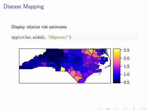
We now examine the variances of the spatial and non-spatialrandom effects.
Recall that the ICAR model variance has a conditionalinterpretation.
To obtain a rough estimate of the marginal variance we obtain theposterior median of the Ui ’s and evaluate their variance.
From the output below, we conclude that the spatial random effectsdominate for the SIDS data so that we conclude there is clusteringof cases in neighboring areas.
Disease mapping
# Extract spatial random effects and calculate# varianceU <- m1$summary.random$ID2[5]var(U)## 0.5quant## 0.5quant 0.1098423# variance of non-spatialm1$summary.hyperpar## mean sd 0.025quant 0.5quant## Precision for ID 17946.354826 1.751483e+04 1204.781841 12805.63061## Precision for ID2 2.299427 8.843653e-01 1.091817 2.12514## 0.975quant mode## Precision for ID 64499.89990 3275.258473## Precision for ID2 4.50051 1.8233581/m1$summary.hyperpar[1, 4]## [1] 7.809065e-05
Virtually all residual variation is spatial.

Clustering via Moran’s I
We evaluate Moran’s test for spatial autocorrelation using the “W”style weight function: this standardizes the weights so that for eacharea the weights sum to 1. Also define the “B” style for later.
To obtain a variable with approximately constant variance we formresiduals from an intercept only model.
library(spdep)# Note the nc.sids loaded from the data() command# is in a different order to that obtained from the# shapefiledata(nc.sids)col.W <- nb2listw(ncCR85.nb, style = "W", zero.policy = TRUE)col.B <- nb2listw(ncCR85.nb, style = "B", zero.policy = TRUE)rm(nc.sids)quasipmod <- glm(SID74 ~ 1, offset = log(EXP74), data = nc.sids2,
family = quasipoisson())sidsres <- residuals(quasipmod, type = "pearson")

Clustering via Moran’s I
moran.test(sidsres, col.W)#### Moran's I test under randomisation#### data: sidsres## weights: col.W#### Moran I statistic standard deviate = 2.4351, p-value = 0.007444## alternative hypothesis: greater## sample estimates:## Moran I statistic Expectation Variance## 0.147531140 -0.010101010 0.004190361
Clustering via Moran’s I
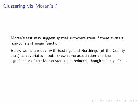
Moran’s test may suggest spatial autocorrelation if there exists anon-constant mean function.
Below we fit a model with Eastings and Northings (of the Countyseat) as covariates – both show some association and thesignificance of the Moran statistic is reduced, though still significant.

Clustering via Moran’s Iquasipmod2 <- glm(SID74 ~ east + north, offset = log(EXP74),
data = nc.sids2, family = quasipoisson())summary(quasipmod2)#### Call:## glm(formula = SID74 ~ east + north, family = quasipoisson(),## data = nc.sids2, offset = log(EXP74))#### Deviance Residuals:## Min 1Q Median 3Q Max## -2.7961 -1.0249 -0.3475 0.6043 4.7261#### Coefficients:## Estimate Std. Error t value Pr(>|t|)## (Intercept) -0.2465437 0.2680159 -0.920 0.35992## east 0.0020105 0.0006469 3.108 0.00247 **## north -0.0028032 0.0014545 -1.927 0.05687 .## ---## Signif. codes: 0 '***' 0.001 '**' 0.01 '*' 0.05 '.' 0.1 ' ' 1#### (Dispersion parameter for quasipoisson family taken to be 2.039456)#### Null deviance: 203.34 on 99 degrees of freedom## Residual deviance: 171.80 on 97 degrees of freedom## AIC: NA#### Number of Fisher Scoring iterations: 4sidsres2 <- residuals(quasipmod2, type = "pearson")nc.sids2$res <- sidsres2

North Carolina SIDS Data: Disease Mapping
par(mar = c(0.1, 0.1, 0.1, 0.1))spplot(nc.sids2, "res")
−2
0
2
4
6
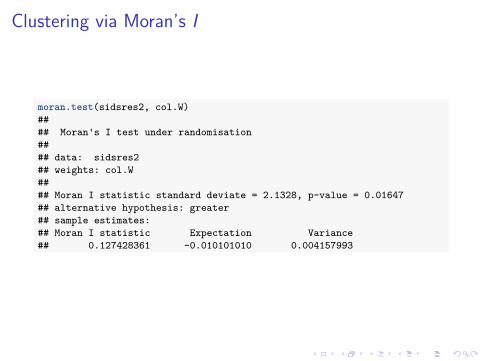
Clustering via Moran’s I
moran.test(sidsres2, col.W)#### Moran's I test under randomisation#### data: sidsres2## weights: col.W#### Moran I statistic standard deviate = 2.1328, p-value = 0.01647## alternative hypothesis: greater## sample estimates:## Moran I statistic Expectation Variance## 0.127428361 -0.010101010 0.004157993
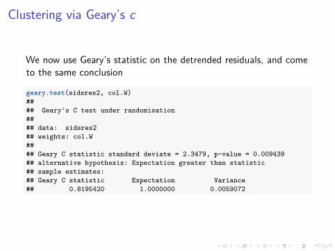
Clustering via Geary’s c
We now use Geary’s statistic on the detrended residuals, and cometo the same conclusion
geary.test(sidsres2, col.W)#### Geary's C test under randomisation#### data: sidsres2## weights: col.W#### Geary C statistic standard deviate = 2.3479, p-value = 0.009439## alternative hypothesis: Expectation greater than statistic## sample estimates:## Geary C statistic Expectation Variance## 0.8195420 1.0000000 0.0059072

Clustering via Moran’s IWe now use Moran’s statistic on the detrended residuals, but withthe binary “B" weight option.
This option has unstandardized weights.
Note the asymmetry in the “W" weights option in the figure below.
The conclusion, evidence of spatial autocorrelation, is the same aswith the standardized weights option.
moran.test(sidsres2, col.B)#### Moran's I test under randomisation#### data: sidsres2## weights: col.B#### Moran I statistic standard deviate = 2.2357, p-value = 0.01269## alternative hypothesis: greater## sample estimates:## Moran I statistic Expectation Variance## 0.125344196 -0.010101010 0.003670354

Clustering via Moran’s IWe now use Moran’s statistic on the detrended residuals, but withthe binary “B" weight option.
This option has unstandardized weights, i.e. weights are all 0 or 1.
Note the asymmetry in the “W" weights option in the figure below.
The conclusion, evidence of spatial autocorrelation, is the same aswith the standardized weights option.
moran.test(sidsres2, col.B)#### Moran's I test under randomisation#### data: sidsres2## weights: col.B#### Moran I statistic standard deviate = 2.2357, p-value = 0.01269## alternative hypothesis: greater## sample estimates:## Moran I statistic Expectation Variance## 0.125344196 -0.010101010 0.003670354

Neighborhood Options
library(RColorBrewer)pal <- brewer.pal(9, "Reds")z <- t(listw2mat(col.W))brks <- c(0, 0.1, 0.143, 0.167, 0.2, 0.5, 1)nbr3 <- length(brks) - 3image(1:100, 1:100, z[, ncol(z):1], breaks = brks,
col = pal[c(1, (9 - nbr3):9)], main = "W style",axes = FALSE)
box()z <- t(listw2mat(col.B))brks <- c(0, 0.1, 0.143, 0.167, 0.2, 0.5, 1)nbr3 <- length(brks) - 3image(1:100, 1:100, z[, ncol(z):1], breaks = brks,
col = pal[c(1, (9 - nbr3):9)], main = "B style",axes = FALSE)
box()

Neighborhood OptionsW style
1:100
1:10
0
Figure 3:

Neighborhood OptionsB style
1:100
1:10
0
Figure 4:

North Carolina SIDS Data: Clustering Conclusions
Both of the Moran’s I and Geary’s c methods suggest that there isevidence of clustering in these data.
The disease mapping model shows that almost all of residualvariation is spatial.

Cluster detection: Openshaw
We implement Openshaw’s method using the centroids of the areasin data.
Circles of radius 30 are used and the centers are placed on a grid ofsize 10.
For multiple radii, multiple calls are required.
The significance level for calling a cluster is 0.002.
library(spdep)data(nc.sids)sids <- data.frame(Observed = nc.sids$SID74)sids <- cbind(sids, Expected = nc.sids$BIR74 * sum(nc.sids$SID74)/sum(nc.sids$BIR74))sids <- cbind(sids, x = nc.sids$x, y = nc.sids$y)# GAMlibrary(DCluster)sidsgam <- opgam(data = sids, radius = 30, step = 10,
alpha = 0.002)

Cluster detection: Openshawplot(sids$x, sids$y, xlab = "Easting", ylab = "Northing")# Plot points marked as clusterspoints(sidsgam$x, sidsgam$y, col = "red", pch = "*")
−200 0 200 400
3750
3900
4050
Easting
Nor
thin
g
************************************************* *******************
**************************************
rm(nc.sids)

Clustering via OpenshawOpenshaw results.sidsgam## x y statistic cluster pvalue size## 1 151.96 3776.92 15 1 1.743356e-03 1## 2 161.96 3776.92 15 1 1.743356e-03 1## 3 171.96 3776.92 15 1 1.743356e-03 1## 4 141.96 3786.92 15 1 1.743356e-03 1## 5 151.96 3786.92 15 1 1.743356e-03 1## 6 161.96 3786.92 15 1 1.743356e-03 1## 7 171.96 3786.92 15 1 1.743356e-03 1## 8 181.96 3786.92 15 1 1.743356e-03 1## 9 131.96 3796.92 15 1 1.743356e-03 1## 10 141.96 3796.92 15 1 1.743356e-03 1## 11 151.96 3796.92 15 1 1.743356e-03 1## 12 161.96 3796.92 15 1 1.743356e-03 1## 13 171.96 3796.92 15 1 1.743356e-03 1## 14 181.96 3796.92 15 1 1.743356e-03 1## 15 131.96 3806.92 46 1 5.531787e-06 2## 16 141.96 3806.92 46 1 5.531787e-06 2## 17 151.96 3806.92 46 1 5.531787e-06 2## 18 161.96 3806.92 23 1 2.042224e-04 2## 19 171.96 3806.92 23 1 2.042224e-04 2## 20 181.96 3806.92 15 1 1.743356e-03 1## 21 121.96 3816.92 31 1 2.612008e-04 1## 22 131.96 3816.92 31 1 2.612008e-04 1## 23 141.96 3816.92 46 1 5.531787e-06 2## 24 151.96 3816.92 54 1 7.116023e-07 3## 25 161.96 3816.92 54 1 7.116023e-07 3## 26 171.96 3816.92 23 1 2.042224e-04 2## 27 181.96 3816.92 23 1 2.042224e-04 2## 28 111.96 3826.92 39 1 8.908653e-05 2## 29 121.96 3826.92 31 1 2.612008e-04 1## 30 131.96 3826.92 31 1 2.612008e-04 1## 31 141.96 3826.92 39 1 3.289935e-05 2## 32 151.96 3826.92 54 1 7.116023e-07 3## 33 161.96 3826.92 54 1 7.116023e-07 3## 34 171.96 3826.92 23 1 2.042224e-04 2## 35 111.96 3836.92 39 1 8.908653e-05 2## 36 121.96 3836.92 39 1 8.908653e-05 2## 37 131.96 3836.92 31 1 2.612008e-04 1## 38 141.96 3836.92 39 1 3.289935e-05 2## 39 151.96 3836.92 39 1 3.289935e-05 2## 40 161.96 3836.92 39 1 3.289935e-05 2## 41 121.96 3846.92 46 1 1.311821e-05 3## 42 131.96 3846.92 38 1 3.687198e-05 2## 43 141.96 3846.92 31 1 2.612008e-04 1## 44 151.96 3846.92 39 1 3.289935e-05 2## 45 161.96 3846.92 39 1 3.289935e-05 2## 46 21.96 3856.92 15 1 2.597729e-07 1## 47 31.96 3856.92 15 1 2.597729e-07 1## 48 41.96 3856.92 19 1 7.521274e-04 2## 49 51.96 3856.92 19 1 7.521274e-04 2## 50 121.96 3856.92 46 1 1.311821e-05 3## 51 131.96 3856.92 38 1 3.687198e-05 2## 52 21.96 3866.92 15 1 2.597729e-07 1## 53 31.96 3866.92 15 1 2.597729e-07 1## 54 41.96 3866.92 19 1 7.521274e-04 2## 55 51.96 3866.92 19 1 7.521274e-04 2## 56 61.96 3866.92 19 1 7.521274e-04 2## 57 31.96 3876.92 15 1 2.597729e-07 1## 58 41.96 3876.92 19 1 7.521274e-04 2## 59 51.96 3876.92 19 1 7.521274e-04 2## 60 61.96 3876.92 19 1 7.521274e-04 2## 61 31.96 3886.92 15 1 2.597729e-07 1## 62 41.96 3886.92 15 1 2.597729e-07 1## 63 51.96 3886.92 19 1 7.521274e-04 2## 64 61.96 3886.92 19 1 7.521274e-04 2## 65 21.96 3896.92 20 1 8.429667e-05 2## 66 31.96 3896.92 20 1 8.429667e-05 2## 67 41.96 3896.92 23 1 2.357357e-04 3## 68 51.96 3896.92 18 1 9.141815e-06 2## 69 261.96 3996.92 28 1 6.259866e-04 2## 70 271.96 3996.92 28 1 6.259866e-04 2## 71 281.96 3996.92 28 1 6.259866e-04 2## 72 251.96 4006.92 18 1 2.157989e-04 1## 73 261.96 4006.92 27 1 3.051285e-06 2## 74 271.96 4006.92 27 1 3.051285e-06 2## 75 281.96 4006.92 27 1 3.051285e-06 2## 76 291.96 4006.92 9 1 7.992992e-04 1## 77 241.96 4016.92 18 1 2.157989e-04 1## 78 251.96 4016.92 18 1 2.157989e-04 1## 79 261.96 4016.92 27 1 3.051285e-06 2## 80 271.96 4016.92 27 1 3.051285e-06 2## 81 281.96 4016.92 27 1 3.051285e-06 2## 82 291.96 4016.92 27 1 3.051285e-06 2## 83 301.96 4016.92 16 1 1.200079e-04 2## 84 241.96 4026.92 22 1 9.930536e-05 2## 85 251.96 4026.92 27 1 3.051285e-06 2## 86 261.96 4026.92 27 1 3.051285e-06 2## 87 271.96 4026.92 27 1 3.051285e-06 2## 88 281.96 4026.92 27 1 3.051285e-06 2## 89 291.96 4026.92 27 1 3.051285e-06 2## 90 301.96 4026.92 16 1 1.200079e-04 2## 91 241.96 4036.92 22 1 9.930536e-05 2## 92 251.96 4036.92 18 1 2.157989e-04 1## 93 261.96 4036.92 27 1 3.051285e-06 2## 94 271.96 4036.92 27 1 3.051285e-06 2## 95 281.96 4036.92 27 1 3.051285e-06 2## 96 291.96 4036.92 27 1 3.051285e-06 2## 97 301.96 4036.92 16 1 1.200079e-04 2## 98 251.96 4046.92 18 1 2.157989e-04 1## 99 261.96 4046.92 27 1 3.051285e-06 2## 100 271.96 4046.92 27 1 3.051285e-06 2## 101 281.96 4046.92 27 1 3.051285e-06 2## 102 291.96 4046.92 9 1 7.992992e-04 1## 103 301.96 4046.92 16 1 1.200079e-04 2## 104 271.96 4056.92 9 1 7.992992e-04 1## 105 281.96 4056.92 9 1 7.992992e-04 1## 106 291.96 4056.92 9 1 7.992992e-04 1

Cluster detection: Besag and Newell k = 20
devtools::install_github("rudeboybert/SpatialEpi")library(SpatialEpi)library(maptools)library(maps)library(ggplot2)library(sp)nc.sids <- readShapePoly(system.file("etc/shapes/sids.shp",
package = "spdep")[1], ID = "FIPSNO", proj4string = CRS("+proj=longlat +ellps=clrk66"))referencep <- sum(nc.sids$SID74)/sum(nc.sids$BIR74)population <- nc.sids$BIR74cases <- nc.sids$SID74E <- nc.sids$BIR74 * referencepSMR <- cases/En <- length(cases)

Cluster detection: Besag and Newell k = 20
getLabelPoint <- function(county) {Polygon(county[c("long", "lat")])@labpt
}df <- map_data("county", "north carolina") # NC region county datacentNC <- by(df, df$subregion, getLabelPoint) # Returns listcentNC <- do.call("rbind.data.frame", centNC) # Convert to Data Framenames(centNC) <- c("long", "lat") # Appropriate Headercentroids <- matrix(0, nrow = n, ncol = 2)for (i in 1:n) {
centroids[i, ] <- c(centNC$lat[i], centNC$long[i])}colnames(centroids) <- c("x", "y")rownames(centroids) <- 1:n

Cluster detection: Besag and Newell k = 20
NCTemp <- map("county", "north carolina", fill = TRUE,plot = FALSE)
NCIDs <- substr(NCTemp$names, 1 + nchar("north carolina,"),nchar(NCTemp$names))
NC <- map2SpatialPolygons(NCTemp, IDs = NCIDs, proj4string = CRS("+proj=longlat"))# Fix currituck county which is 3 islandsindex <- match(c("currituck:knotts", "currituck:main",
"currituck:spit"), NCIDs)currituck <- list()for (i in c(27:29)) currituck <- c(currituck, list(Polygon(NC@polygons[[i]]@Polygons[[1]]@coords)))currituck <- Polygons(currituck, ID = "currituck")

Cluster detection: Besag and Newell k = 20
# make new spatial polygons objectNC.new <- NC@polygons[1:(index[1] - 1)]NC.new <- c(NC.new, currituck)NC.new <- c(NC.new, NC@polygons[(index[3] + 1):length(NC@polygons)])NC.new <- SpatialPolygons(NC.new, proj4string = CRS("+proj=longlat"))NCIDs <- c(NCIDs[1:(index[1] - 1)], "currituck", NCIDs[(index[3] +
1):length(NC@polygons)])NC <- NC.new

Cluster detection: Besag and Newell k = 20
# SANITY CHECK: Reorder Spatial Polygons of list to# match order of countynames <- rep("", 100)for (i in 1:length(NC@polygons)) names[i] <- NC@polygons[[i]]@IDidentical(names, NCIDs)## [1] FALSE
index <- match(NCIDs, names)NC@polygons <- NC@polygons[index]rm(index)
names <- rep("", 100)for (i in 1:length(NC@polygons)) names[i] <- NC@polygons[[i]]@IDidentical(names, NCIDs)## [1] TRUE
Cluster detection: Besag and Newell k = 20
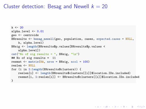
k <- 20alpha.level <- 0.01geo <- centroidsBNresults <- besag_newell(geo, population, cases, expected.cases = NULL,
k, alpha.level)BNsig <- length(BNresults$p.values[BNresults$p.values <
alpha.level])cat("No of sig results = ", BNsig, "\n")## No of sig results = 11resmat <- matrix(NA, nrow = BNsig, ncol = 100)reslen <- NULLfor (i in 1:length(BNresults$clusters)) {
reslen[i] <- length(BNresults$clusters[[i]]$location.IDs.included)resmat[i, 1:reslen[i]] <- BNresults$clusters[[i]]$location.IDs.included
}

Cluster detection: Besag and Newell k = 20
par(mfrow = c(3, 3), mar = c(0.1, 0.1, 0.1, 0.1))for (i in 1:6) {
plot(NC.new)plot(NC.new[resmat[i, c(1:reslen[i])]], col = "red",
add = T)}
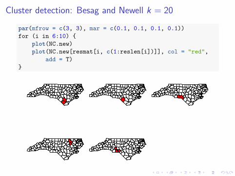
Cluster detection: Besag and Newell k = 20
par(mfrow = c(3, 3), mar = c(0.1, 0.1, 0.1, 0.1))for (i in 6:10) {
plot(NC.new)plot(NC.new[resmat[i, c(1:reslen[i])]], col = "red",
add = T)}

Cluster detection: SatScan
# Kulldorffpop.upper.bound <- 0.2n.simulations <- 999alpha.level <- 0.05Kpoisson <- kulldorff(geo, cases, population, expected.cases = NULL,
pop.upper.bound, n.simulations, alpha.level, plot = T)Kcluster <- Kpoisson$most.likely.cluster$location.IDs.included

Cluster detection: SatScanMonte Carlo Distribution of Lambda
log(λ)
Fre
quen
cy
2 4 6 8 10 12 14
010
020
030
0 Obs. log(Lambda) = 13.661p−value = 0.001
Figure 5:

Cluster detection: SatScanplot(NC.new, axes = TRUE)plot(NC.new[Kcluster], add = TRUE, col = "red")title("Most Likely Cluster")
84°W 82°W 80°W 78°W 76°W
33°N
34°N
35°N
36°N
37°N
Most Likely Cluster
Figure 6:

Cluster detection: SatScan
Now look at secondary clusters.
Two are significant, and indicated in Figures below
K2cluster <- Kpoisson$secondary.clusters[[1]]$location.IDs.includedplot(NC.new, axes = TRUE)plot(NC.new[K2cluster], add = TRUE, col = "red")title("Second Most Likely Cluster")

Cluster detection: SatScan
84°W 82°W 80°W 78°W 76°W
33°N
34°N
35°N
36°N
37°N
Second Most Likely Cluster
Figure 7:

Bayes cluster model
# Load NC map and obtain geographic centroidslibrary(maptools)sp.obj <- readShapePoly(system.file("etc/shapes/sids.shp",
package = "spdep")[1], ID = "FIPSNO", proj4string = CRS("+proj=longlat +ellps=clrk66"))centroids <- latlong2grid(coordinates(sp.obj))

Bayes cluster model
y <- sp.obj$SID74population <- sp.obj$BIR74E <- expected(population, y, 1)max.prop <- 0.15k <- 5e-05shape <- c(2976.3, 2.31)rate <- c(2977.3, 1.31)J <- 7pi0 <- 0.95n.sim.lambda <- 0.5 * 10^4n.sim.prior <- 0.5 * 10^4n.sim.post <- 0.5 * 10^5output <- bayes_cluster(y, E, population, sp.obj, centroids,
max.prop, shape, rate, J, pi0, n.sim.lambda, n.sim.prior,n.sim.post)
## [1] "Algorithm started on: Tue Jul 21 10:42:33 2015"## [1] "Geographic objects creation complete on: Tue Jul 21 10:42:33 2015"## [1] "Importance sampling of lambda complete on: Tue Jul 21 10:42:35 2015"## [1] "Prior map MCMC complete on: Tue Jul 21 10:42:37 2015"## [1] "Posterior estimation complete on: Tue Jul 21 10:43:55 2015"

Bayes cluster model
SMR <- y/Eplotmap(SMR, sp.obj, nclr = 6, location = "bottomleft",
leg.cex = 0.5)plotmap(output$prior.map$high.area, sp.obj, nclr = 6,
location = "bottomleft", leg.cex = 0.5)plotmap(output$post.map$high.area, sp.obj, nclr = 6,
location = "bottomleft", leg.cex = 0.5)barplot(output$pj.y, names.arg = 0:J, xlab = "j", ylab = "P(j|y)")plotmap(output$post.map$RR.est.area, sp.obj, log = TRUE,
nclr = 6, location = "bottomleft", leg.cex = 0.5)

Bayes cluster model
84°W 82°W 80°W 78°W 76°W
33°N
34°N
35°N
36°N
37°N
0 − 0.7880.788 − 1.581.58 − 2.362.36 − 3.153.15 − 3.943.94 − 4.73
Figure 8: SMRs

Bayes cluster model
84°W 82°W 80°W 78°W 76°W
33°N
34°N
35°N
36°N
37°N
0.000153 − 0.001810.00181 − 0.003470.00347 − 0.005130.00513 − 0.006790.00679 − 0.008450.00845 − 0.0101
Figure 9: Prior probabilities of lying in a cluster

Bayes cluster model
84°W 82°W 80°W 78°W 76°W
33°N
34°N
35°N
36°N
37°N
4.83e−08 − 0.1650.165 − 0.330.33 − 0.4960.496 − 0.6610.661 − 0.8260.826 − 0.991
Figure 10: Posterior probability of a cluster

Bayes cluster model
0 1 2 3 4 5 6 7
j
P(j|
y)
0.0
0.2
0.4
0.6
Figure 11: Posterior on the number of clusters

Bayes cluster model
84°W 82°W 80°W 78°W 76°W
33°N
34°N
35°N
36°N
37°N
0.489 − 0.6720.672 − 0.9230.923 − 1.271.27 − 1.741.74 − 2.42.4 − 3.3
Figure 12: Posterior relative risk estimates
Related Documents