Sir! I’d Rather Go to School, Sir!

Sir! I’d Rather Go to School, Sir!∗

Mahdi Majbouri†

Babson College

Abstract

Would the fear of conscription entice the youth to get more education despite their

will? This paper uses a discontinuity in the military service law in Iran to answer this

question. Iranian males become eligible for military service when they reach 18. But,

between 2000 and 2010, sole sons whose fathers’ age was over 58, at the time of son’s

eligibility, were exempted from the service. Sole sons whose fathers’ age is a bit below

the threshold may stay in school until their father reaches (or passes) 59, in order to

get exemption after leaving school. This study shows that, as a result of this, there is a

discontinuity in education levels of sole sons at the father’s age of 59. Sole sons whose

fathers’ age was below the threshold are 13 percentage points (20 percents) more likely

to attend college than those whose fathers’ age was above it. This exogenous increase

is used to estimate returns to college education in Iran.

JEL Code: J31, J47

Keywords: Conscription, Coercive labor market, Natural experiment, Regression dis-

continuity, Higher-educational attainment

∗For their comments and suggestions on an earlier version of this paper, the author wishes to thankKristin Butcher, Patrick J. Ewan, Pinar Keskin-Bonatti, and other attendants of the Wellesley CollegeEconomics department brown-bag lunch series, as well as Erica Field, Jacob Shapiro, Thomas Pepinsky,and the participants of the AALIMS 2015 conference at Princeton University, and the UNU-WIDER 2015conference on Human Capital and Growth, at Helsinki. Sincere thanks go to Claire S. Jacobs and SigridSommerfeldt, for reviewing this manuscript. All the remaining errors are mine.†Correspondence to: Mahdi Majbouri, Babson College, Economics Division, 231 Forest St., Wellesley,

MA 02457, USA; [email protected]; phone: 781-239-5549

1

1 Introduction

96 out of 99 countries that experienced internal armed conflict between 1946 and 2014 are

developing countries.1 Moreover, at least one side of all 122 interstate armed conflicts in

the same period has been a developing country.2 These show that in developing countries,

having a strong and yet relatively inexpensive army is critical for the state. Military service,

which is mandatory in over 60 countries around the world (Chartsbin, 2011), is a relatively

inexpensive way that governments use to recruit for their armed forces. Yet, its compulsory

nature remains controversial.

Despite the prevalence and importance of conscription, its different aspects and con-

sequences, particularly in developing countries and at the time of peace, have remained

under-researched.3 As one of the few studies on this topic, this paper uses a novel natural

experimental setting to document whether and how much (if any) the compulsory nature

of military service is abhorred in a developing country, at the time of peace. The results

draw on some of the fundamental pillars of economic science, incentives, decision making,

and inefficiency and use data from one of the most understudied developing countries, Iran.

In Iran, military service for males 18 and above is compulsory. But in some cases exemp-

tion is possible. For instance, certain disabilities and chronic conditions make one eligible for

permanent exemption. College and graduate students are also exempted (temporarily) from

the service during their studies. But, one particular case of exemption is that of a sole son.

Between 2000 and 2011, a sole son could get exemption to take care of his elderly father,

if his father was 59 or older (over 58) when he had reached his 18th birthday and became

1The three developed countries are France, Spain and United Kingdom. Source is author’s calculationfrom UCDP/PRIO Armed Conflict Dataset, Version 4-2015. The dataset is provided by Uppsala ConflictData Program (UCDP) and Center for the Study of Civil Wars, International Peace Research Institute,Oslo (PRIO). See Gleditsch et al. (2002), Pettersson and Wallensteen (2015), and Themner (2015) for thedescription of the dataset. In this dataset, an armed conflict (internal or interstate) is defined as “a contestedincompatibility that concerns government and/or territory where the use of armed force between two parties,of which at least one is the government of a state, results in at least 25 battle-related deaths.” For a morein-depth discussion on definitions, see http://www.pcr.uu.se/research/ucdp/definitions/.

2Source is author’s calculation from UCDP/PRIO Armed Conflict Dataset, Version 4-2015. For a defini-tion of conflict, as well as information on data, see footnote 1.

3As will be discussed, most of the literature is about developed countries and draft at the time of war.

2

eligible for the military service.4 This means those sole sons whose fathers are younger may

miss this opportunity. But they have a way to benefit from this exemption as well. An 18

year-old sole son whose father’s age is below but close to 59, can get temporary exemption

(like everyone else) by going to school (i.e. college) for a few years, and postpone his con-

scription. In the meantime, his father will reach (or pass) the age of 59, as a result of which

he can get exemption. Therefore, those 18 year-old sole sons whose fathers’ age is above 58

(59 or older) have less incentive to continue their education than those whose father is 58 or

younger.

This study establishes that, in Iran, there is a discontinuity in college attainment rate of

sole sons, whose fathers’ age was over 58 when they were 18 years old, relative to the sole sons

with slightly younger fathers. The size of this discontinuity is at least about 13 percentage

points (20 percent). As a robustness check, this study shows that there is no discontinuity in

college attainment among the sisters of sole sons, or the sons and daughters of multiple-son

households. Since the military exemption law should not affect any of these groups except

the sole sons, the results provide strong evidence that military exemption law created such

discontinuity. In other words, fear of conscription entices sole sons to gain more education

despite their will. If there had not been such an exemption law, sole sons of younger fathers

would not have attended college. This exogenous increase in college attendance may be used

to estimate returns of college on various outcomes, such as wages. But, because of data

limitations this exogenous increase turns out to be a weak instrument and the IV estimates

are not reliable.

By showing that individuals are willing to get education despite their will to avoid con-

scription, this study provides evidence for the inefficiency of conscription. But, moreover, it

offers a lower bound (minimum) for the size of these inefficiencies.

There have been many studies on the impact of conscription in developed countries, and

4The required age of father has increased to 65 in 2012 and then to 70 in 2014. Later, the age requirementwas abrogated and replaced with a father’s disability that impedes him from working. This has remainedthe law until now that this paper is written.

3

almost all during the war time. Angrist (1990) is a seminal work that uses Vietnam draft

lottery as a natural experiment since draft-eligible individuals were conscripted based on

randomly chosen birth-days. Most studies that come later (and all cited here) use the same

natural experiment. Angrist (1990) studies the effect of conscription at war time on earnings

of US veterans later in life. He finds 15% lower earnings for veterans vs. non-veterans

in 1970s and 80s. Angrist et al. (2011), however, revisit the question 20 years later and

surprisingly find that the gap between veterans and non-veterans earnings disappeared by

the early 1990s. Angrist and Chen (2011) attribute this to flattening of wages in mid-life and

increase in schooling of veterans due to Vietnam War GI Bill. Autor et al. (2011), on the

other hand, find a decline in employment and a rise in disability receipts by Vietnam War

Veterans (particularly for Post-Traumatic Stress Disorder) in 2000s. This is while Angrist

et al. (2010) found no evidence of either one in 1990s. Conley and Heerwig (2012) find that

interestingly, there is no impact of draft on post war mortality of veterans vs. non-veterans

in the long-run. Siminski and Ville (2011) find the same results for Australian veterans who

were drafted during the Vietnam War. All studies on various impacts of the Vietnam-era

draft (and there are many5), inevitable use this draft which was during a war. Therefore,

it is hard to disentangle the effect of the war vs. the effect of conscription in these studies.

They remain silent about the effect of conscription during peacetime.

There is very little research on the impacts of conscription in peacetime on various out-

comes and markets, such as human capital accumulation (cognitive and non-cognitive skills,

educational attainment, and health), earnings, hours worked, labor markets, and marriage

markets. Two studies that stand out are Bauer et al. (2012) and Card and Cardoso (2012).

Using regression discontinuity, Bauer et al. (2012) compare cohorts who were born before

July 1, 1937 in Germany and hence exempted from service in 1950s with those who were

5For example, Schmitz and Conley (2016) find that “veterans with a high genetic predisposition forsmoking were more likely to have been smokers, smoke heavily, and are at a higher risk of being diagnosedwith cancer or hypertension at older ages.” They also find that the effect is smaller among those who went tocollege after the war. Conley and Heerwig (2011) study the impact of the same draft on residential stability,housing tenure, and extended family residence after the War and find mixed results.

4

born right after (who had to serve in 1950s). They find no effect of conscription on wages

later in life. Interestingly, in a different design, Card and Cardoso (2012) also find no effect

of conscription on Portuguese with more than primary education, although they find positive

impact on less educated individuals.

These studies are about developed countries. Nevertheless, one wonders if conscription

has no effect on earnings (in those countries) or positive effect in the case of less educated

Portuguese, how much people are willing to avoid it. This study embarks to answer this

question. Card and Lemieux (2001) answer a similar question: whether people were willing

to go to college to avoid draft during the Vietnam War. But, they again look at a draft

during a war, while this paper is about draft during peacetime. It is not very surprising to

see people were willing to go to college to avoid a war. But, it is interesting to know whether

people do that in peacetime, in a developing country where supply of college education is

limited and entering college is very competitive and costly. Moreover, as Card and Lemieux

(2001) explain, they “find a strong correlation between the risk of induction faced by a cohort

and the relative enrollment and completed education of men.” This study, however, finds a

causation.

The rest of the paper is structured as follows. Section 2 explains the military service

and its exemption laws in Iran. It also explains the identification strategy. The data are

discussed in Section 3 after which the estimation and results are depicted in Section 4. The

conclusion discusses policy implications for countries with military service laws.

2 Military Service in Iran

Conscription, in its modern form, was first introduced by the French Republic in the wars

after the French Revolution6 to protect the country from the attacks of other European pow-

ers. Later, however, it made the French army one of the most powerful military in the early

6Britannica Academic, s.v. “Conscription,” accessed August 13, 2016,http://academic.eb.com.ezproxy.babson.edu/levels/collegiate/article/25932#.

5

1800s. With the rise of nationalism in Europe and the rest of the world in the 19th century,

this system became popular with the governments around the world to create and maintain

an army.7 In recent decades, however, criticism from various angles (religious, philosophical,

economic8, political, and human rights grounds9) made conscription controversial. Moreover,

after the end of the cold war and with the advances in military technology, which reduced the

need for large armies10, many states abandoned this system and began to rely on professional

armies and volunteers.11

In Iran, mandatory military service for men was first introduced in 1924 by Reza Shah,

the king at the time, to the Parliament and, despite some opposition, became the law.12

After the Islamic Revolution of 1979, this law was modified in 1984 (in the middle of Iran-

Iraq War), and stated that conscription consists of 30 years and is divided into four periods:

First, a two-year period in which every male whose 18th year of life is completed (aged 18 and

in his 19th year of life) has to participate in military training and activities.13 The training

7Interestingly, the Prussian system of conscription, developed during the Napoleonic wars, became themodel for other European nations. France which abandoned conscription after Napoleon’s defeat in 1815,re-instituted it later with some restrictions. But, it reverted back to universal conscription after the defeatfrom the large conscripted German army, in the Franco-German War (1870-71). Russia, and later the SovietUnion, have had some form of conscription for most of the last two centuries. United States and Britainare two Western powers that tried to avoid conscription for most of the 19th and 20th centuries, except atthe time of the US Civil War, and the two World Wars (Britannica Academic, s.v. “Conscription,” accessedAugust 13, 2016, http://academic.eb.com.ezproxy.babson.edu/levels/collegiate/article/25932#.) One of theearly examples of conscription in developing countries is its introduction by Muhammad Ali (the OttomanAlbanian ruler of Egypt) in early 19th century in Egypt.

8For a thorough discussion of economics of conscription vs. all-volunteer force, see Warner and Asch(2001). They also offer empirical evidence that the arguments for all-volunteer force in the US are substan-tially stronger in 2001 than they were in 1973, when conscription was abolished.

9One may challenge military service on other dimensions as well. For instance, using draft lottery inArgentina, Galiani et al. (2011) show that conscription increased the chance of development of criminalrecord.

10There has been a complementarity between capital and labor in military in all human history even withsome modern technologies. For instance, guns need soldiers and tanks need drivers and gunners and viceversa. The advanced military technologies, such as smart drones, make capital more of a substitute for laborrather than a complement. This reduces the need for labor in the armies. Moreover, some military tech-nology that have considerable destructive capabilities cannot be confronted with armies of regular soldiers.Therefore, return to regular soldiers has been declining over time, which has reduced the need for largestanding armies.

11For a review of studies on recruitment, retention, military experience and productivity in the All-Volunteer Force (AVF) era in the United States, see Warner and Asch (1995).

12From 1906 to the Islamic Revolution of 1979, Iran had been a constitutional monarchy with a parliament.13The two-year training and service period has recently changed to 21 months.

6

lasted for three months and the other twenty one months were spent in service to the armed

forces (military and police). After that, there are three consecutive “reserve” periods: an

eight-year period, called “priority reserve” followed by two ten-year periods, “first reserve”

and “second reserve”. In these reserve periods, those who finished the two-year military

training and service are on reserve and would be called to service if needs arise (for example,

if the country goes to war). The priority would be given to those who are on the priority

reserve, and then the first and second reserves respectively.

According to law, those who are medically unfit for the service (those with some dis-

abilities and chronic illnesses) are exempted. Tertiary level students are also exempted from

military service as long as they are in school. Students cannot stay in school more than a

certain number of years depending on the degree they pursue (Bachelor, Master, and Ph.D.).

Upon leaving the tertiary level institutions, they need to go to military service. Another

form of exemption, which is a basis of this paper, is given to the only sons whose fathers are

59 or older14 at the time of conscription. The argument is that the elderly father may need

his sole son’s assistance in the old age.15

2.1 Exemption and Education

This paper uses a combination of the sole son and student exemptions laws to identify a

discontinuity in educational attainment. Consider a male who is 18 years old and is the only

son but his father is 55 to 58 years old. He is just one to four years short of the threshold

needed for exemption by the law. But he can take advantage of the student exemption law

and go to college for four years so that he gets (temporary) student exemption in those years.

After he finishes his college (or even in the middle of it), his father is over 58 and he becomes

1459 was the threshold for father’s age until 2012. It has changed to 65 in 2012 and then to 70 in 2014.15There are other exemptions as well: 1) men who are the sole child of their parents, 2) men who are the

sole caregiver of a physically or mentally disabled parent, sibling, or second line family members, 3) doc-tors, firefighters, and other emergency workers whose military service may jeopardize health and emergencyservices, 4) employees of important governmental agencies that directly or indirectly assist the military areexempt at the time of war, 5) employees of businesses that work with the military are exempt from serviceat the time of war, 6) prisoners.

7

eligible for the sole son exemption. Compare him with someone who is 18 years old and is

the only son of a father who is 59 and older. This second man does not need to go to college

to get exemption. Therefore, those sole sons whose fathers’ age is below the threshold, when

they are 18, have more incentive to go to college or grad school and those whose fathers’

age is above have less. This may provide a discontinuity in educational attainment for the

sole sons whose fathers are younger and older than 58. Therefore, we can use regression

discontinuity method to estimate the effect of exemption law on educational attainment.

3 Data

In this study and for the reasons explained below, I use the 2% random and nationally

representative sample of the 2011 Census of Iran. Statistical Center of Iran (SCI) is the

main organization in charge of gathering micro datasets in Iran. It has been collecting the

national census every ten years starting in 1956 and every five years since 2006.16 The

latest one available to me is the 2011 census. The military exemption law for age 59 was

implemented between 2001 and 2011. The 2011 census has individuals that were affected

throughout the whole period. This is one advantage of this dataset.

The 2011 census provides basic demographic data on age, education, labor market par-

ticipation, marital status, employment status, relationships within the household, as well as

the number of children ever born, and pregnancy in the 12 months prior to the survey. It also

contains information on the household’s dwelling and its amenities. It does not, however,

have information on the labor market outcome such as income and hours worked.

Education, which is the most important variable in this study, is reported with codes.

Unfortunately, often times than not, each code represents more than one grade. For example,

there is one code assigned to several grades of high school. Therefore, it is not possible to

find the years of education attained from these codes. But it is possible to identify the level

of education, i.e. primary, middle school, high school, and college and above. Hence, in

16The censuses are 1956, 1966, 1976, 1986, 1996, 2006, and 2011.

8

this study, only a dummy, that is equal to one when an individual attained college or above

and zero otherwise, is defined and used as the main dependent variable. The number of

years of college or graduate school attended is not observed. Education code is not reported

for individuals who are illiterate. But whether an individual is literate or not is observed

in the census.17 When one defines the college dummy variable, she should make sure that

the dummy for college education is zero for the illiterate even though the education code is

missing for them.

Age is another important variable in this study which is measured in years. I use the age

of father when the sole son was 18 to identify whether the exemption law would apply to the

sole son or not. If the father is younger than 59 (i.e. 58 or younger), the law applies to his

sole son.18 In other words, the discontinuity in the exemption law starts at the end of age 58,

just when the father becomes 59. In this study, sole sons whose father’s age was in a range

around 5919 when they were 18 are studied. This is a very small sample of the population.

Therefore, one needs a dataset with many observations to be able to have enough number

of sole sons with fathers in that age range. The fact that the 2011 has over 1.5 million

observations is another advantage of this dataset over other Iranian datasets.

One may argue that age is a variable for which “bunching” at certain values happens.

That is people are more likely to round their age to the closest multiple of 5. For example,

people aged 58, 59, or 61 are likely to report their age as 60. Therefore, usually in surveys,

the number of observations with ages that are multiples of 5 (like 40, 45, 50, etc.) is

larger than the number of observations with ages around those multiples. For example, the

number of observations with age 60 is larger than those with age 58, 59, or 61. But, here,

we are considering the age of father when the child was 18 not the age of father reported in

the survey. Therefore, bunching should not happen, particularly around the discontinuity

17A dummy variable is in the census that is one for the literate and zero otherwise.18Unless the son goes to college and postpone his illegibility for military service until his father becomes

older than 58 (59 or older).19The main age range used is 49 to 68 (±10 years around the threshold). Other age ranges used for

robustness check are 53 to 64 (±6), 51 to 66 (±8), 47 to 70 (±12), and 44 to 73 (±15).

9

threshold. Moreover, the distribution of father’s age when the child was 18 changes smoothly

in the sample and there is no evidence of bunching.

From the discussion on age, it is clear that we need to be able to identify fathers and

sole sons. This is not easy to achieve, since the demographic information in the data set

is very basic. None of the Iranian datasets identify a child’s father in the household. The

best variables that can be used to identify fathers (and other household members) are the

relationship to the head, and gender. The relationship to the head variable helps us identify,

the head’s spouse, the children of the head, the other relatives of the head who live with

the household including in-laws, and non-relatives. Using this variable, we can identify

households that only consist of a male head, his spouse, and his children. Obviously, male

heads in those households are fathers of individuals reported as their children. In the rare

case that the head of the household is reported as female and her spouse is male (0.2% of the

households), the spouse can be both the father or step-father. Therefore, those households

are not considered. In households that have extended family members, particularly multiple

generational households (households with grandfathers their children and grand children), it

is not possible to accurately identify fathers .

One issue with all Iranian datasets is that only the children present in the household are

recorded in the data and those who left the household for any reason (studying in another

place or marriage) are not in the data. This makes identifying the only sons difficult. For

example, a household who seems to have one son in the data, may actually have two or

more. The other son(s) left the household after marriage or to go to college in the city.

The 2011 census, however, asks for the number of children ever born by a mother (this is

another advantage of the 2011 census over other Iranian data sets.) It also asks who each

person’s mother is in the household. Using these two questions one can restrict the sample

to households whose children are all present. In order to do that, first, I restrict the sample

to households that only consist of a male head and his spouse and the children of the head.

In these households, only one mother is present. Then, we identify the number of children

10

who are present in the household and belong to the mother. We also know the number

of children the mother has ever born. Only households for which these two numbers are

the same are considered. These are the households that do not have children who left the

household. Therefore, it is possible to identify sole sons in them with accuracy. We focus on

these households. Table 1 shows the number of different types of households in the census

data including the final sample that is used.

It is unlikely that this algorithm identifies individuals who are not sole sons as sole sons.

But if that happens, this inaccurate identification of sole sons happens on both sides of

the threshold and hence does not bias the regression discontinuity results in favor of the

hypothesis. In other words, it does not create an effect when there is no effect. In fact,

measurement error in identification of sole sons creates a noisy estimate (larger standard

errors) and an under-estimation of the true effect of the military service law.

In rural areas, the size of the sample of sole sons (identified by the way that was explained

above) is quite small and inadequate to get statistical power. This is because of two reasons:

1) we need to identify sole sons, aged 19 and over, from the sample of households whose

all children are present. But, rural children (especially in this age range) are substantially

more likely not to be present in the household or have siblings who are not present in the

household, than their urban counterparts. They leave the household to migrate (temporarily

or permanently) to urban areas.They also marry earlier. 2) In 2011, less than 30% of the

population was living in rural areas. This means the size of the urban population was more

than twice the size of the rural population. As a result of these two reasons, fewer sole sons

can be identified in rural areas.

Even if we have enough number of sole sons in rural areas to get statistical power, we still

cannot identify the true effect of exemption law on college attainment rates in rural areas.

This is because almost all college-educated (or college-enrolled) rural children went (or go)

to college in a city (not in the village) and usually stay there after graduation. In other

words, most the college-educated or college student sole sons have already left the household

11

and are not part of the sample. As a result, we do not observe them to be able to measure

the impact of policies on the college attainment rates in rural areas. For all these reasons,

in this study, we only focus on urban areas.20

Another concern that one may have is measurement error in father’s age. Since we are

interested in discontinuity close to a threshold of father’s age, measurement error in age close

to the threshold can easily take an observation from one side to the other side. This can

happen on both sides of the threshold but it only increases the standard error of the estimate

and produces an under-estimation of the true effect.

Table 2 reports the summary statistics of the variables in six samples: 1) Sole sons

(top-left panel), 2) Sisters of sole sons (top-right panel), 3) Sons in multiple-son households

(mid-left panel), 4) Daughters in multiple-son households (mid-right panel), 5) All men aged

19 to 28 (bottom-left panel), 6) All women aged 19 to 28 (bottom-right panel). Since the

military exemption law was applied between 2001 and 2010, in the 2011 census, the sole

sons are 19 to 28 years old. Therefore, all samples used in this study and reported in Table

2 are in the same age range. As can be seen the sample of sole sons and their sisters are

different from the general population (the bottom panel). They are slightly younger but

substantially more educated. Therefore, the results found in this study are Local Average

Treatment Effects (LATE) and may not be generalized to the population.

4 Estimations and Robustness Checks

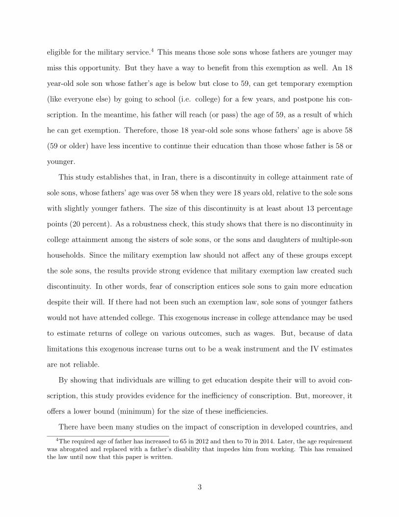
As explained in Section 2.1, because of the exemption law, we expect that sole sons whose

fathers were 58 or younger (when they were 18) attend college more than those whose fathers

were older than 58. This means that there should be a discontinuity in the college attainment

rate right after the father’s age of 58. This section documents this discontinuity and discusses

its consequences. Figure 1 documents the discontinuity in college attainment of the sole sons

20The results for rural areas are mostly statistically insignificant.

12

whose father’s age was between 49 and 68 when they were 18 years old, in urban areas21.

The figure has three sub-figures showing linear, quadratic, and polynomial fit of the data.

The horizontal axis shows the age of father when his sole son was 18 and the vertical axis

is the share of sole sons who attended college and above. The solid lines are the fitted lines

and the light gray lines show the 95% confidence interval. The dots represent the average

college attendance rate at each father’s age. The discontinuous decline in college attendance

rate right after age 58, in all specifications in Figure 1, is evidence for the impact of the

exemption law.

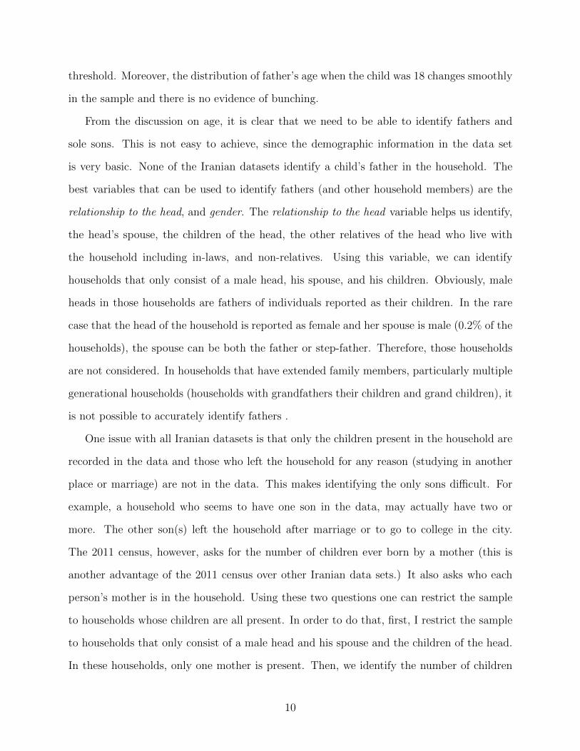
We do not expect the exemption law to affect girls. So for robustness check, we can draw

a similar figure as Figure 1 for sisters of sole sons. Since sisters of sole sons are living in the

same household (have the same parents and face a somewhat similar environment), they are

a good comparison group. Figure 2 is drawn similar to Figure 1, but for these sisters. The

horizontal axis is the age of a father who has a sole son when his daughter (sole son’s sister)

was 18 and the vertical axis is the share of sole sons’ sisters who attended college and above.

The figure does not show any discontinuity in college attainment rate for sisters of sole sons

right after the father’s age of 58. This provides further evidence that it was the exemption

law that affected college attainment of sole sons at father’s age of 58 or less, and not any

other factor (particularly those that could have affected their sisters too).

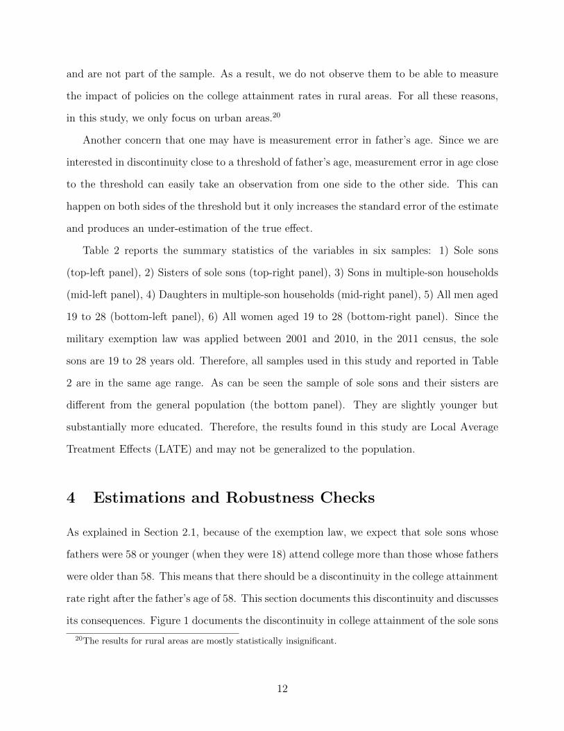
To further strengthen the result we can also check to see if the exemption law had any

impact on sons in households who have multiple sons. The law should not affect college

attainment rates of these sons. Figure 3 shows that this is the case. Although it may seem

that there was a decline, there is no statistically significant discontinuity in college attendance

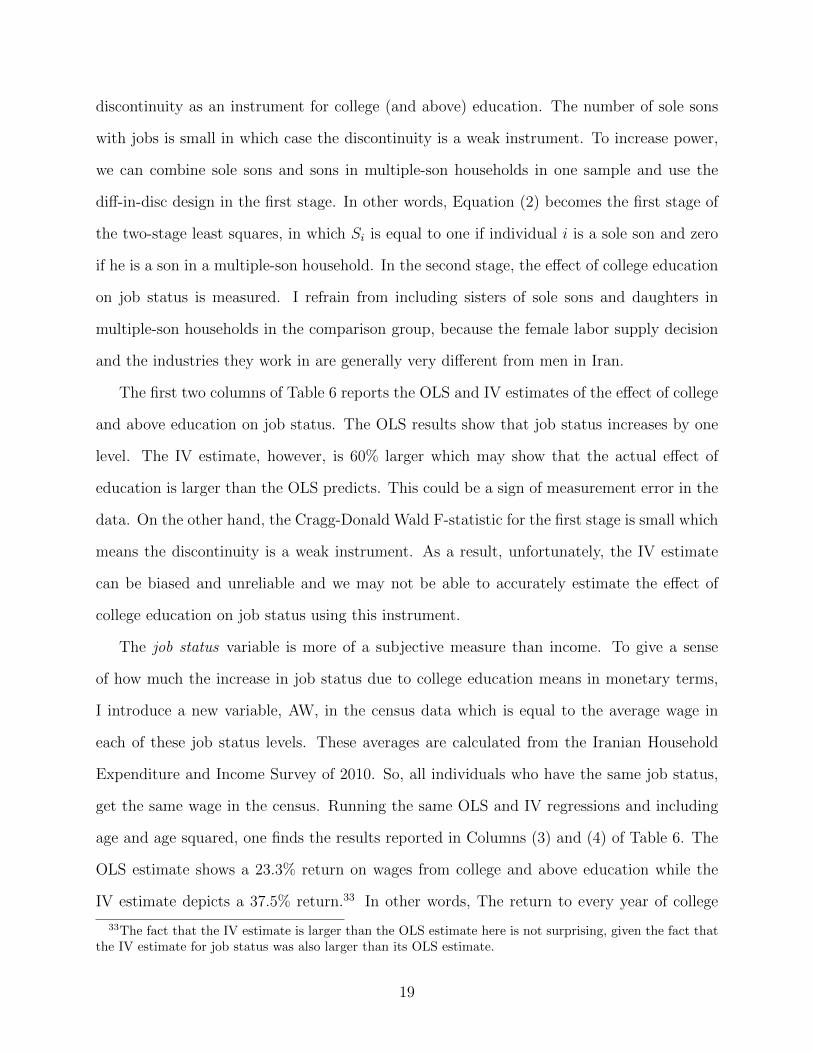
rate for this group just after age 58. Similarly, one expects that the exemption law does not

affect daughters in households with multiple sons. Figure 4 is indeed the evidence for that.

The fact that only sole sons (and not the other three groups) have a discontinuity in college

attainment at the threshold is a strong evidence that military service exemption law caused

21As explained in Section 3, we only focus on the urban areas, because the sample of sole sons for ruralareas is small and selected.

13

it.

We can formalize these figures in regressions as follows:

Yi = α + τDi +l∑

k=1

γk(pi − 58)k +l∑

k=1

δkDi(pi − 58)k + ui, l = 1, 2, 3 (1)

in which Yi is the college attendance for individual i. It is a dummy equal to one if the

individual attended (or is attending) college or higher levels of education and zero otherwise.

Di is a dummy equal to one if individual i’s father was 58 and younger when he/she was

18 and zero if the father’s age was 59 and more.22 The running variable in this regression

discontinuity setting is father’s age when individual i was 18 and it is represented by pi.23

The regressions contain a polynomial of (pi− 58) with degree l.24 l is equal to one, two, and

three. The Local Average Treatment Effect (LATE) is τ .

Table 3 reports the results for Sole sons (left panel), sisters of sole sons (middle panel)

and sons in multiple-son households (right panel).25 The running variable, pi, in the sample

extends from 49 to 58 (i.e. ±10 years from the threshold). In other words, the samples

include individuals whose fathers were between the age of 49 and 68 when they were 18.26 pi

is a discrete rather than a continuous variable. Lee and Card (2008) and Lee and Lemieux

(2010) argue that when the running variable is discrete, correlation in standard errors should

be “clustered” at values of the discrete running variable. Therefore, all regressions correct

for robust heteroskedastic standard errors and correlation inside those clusters. The first

column of Table 3 explores college attendance for sole sons in a linear setting (l = 1 in

Equation (1)). The coefficient of D is positive and significant showing that sole sons whose

fathers’ age was 58 and slightly below when they were 18, have about 13 percentage points

22Other age ranges were analyzed as well and their results reported in Table 3. See footnote 19 .23p is chosen to denote this variable since it is the first letter of the Latin word pater and the Persian word

pedar , both meaning father.24The effect is the difference between actual and counterfactual at the threshold. Since the law affected

sole sons with father’s age of 58 not 59, we are interested in finding the counterfactual at the father’s age of58. This is why pi is subtracted from 58 in the regression.

25The results for daughters in multiple-son households are not reported because of limited space but areavailable upon the request.

26We change the range of the sample in Table 4 and get similar results.

14

more chance of attending college than those whose fathers’ age was 59 and slightly more.

Since the average college attainment rate for the sample of sole sons is 66% (see Table 2),

the effect translates as a 20 percent increase.

Columns (2) and (3) report the quadratic and third-degree polynomial settings. The

coefficient of D remains statistically significant in those settings. It also increases in size

to 0.23 and 0.33 which translate into the LATE of 23 and 33 percentage points (35 and 50

percents respectively). For robustness check, one can run similar regressions for sole sons’

sisters. The results are reported in the middle panel of Table 3. All showing that there is no

evidence of discontinuity in college attendance for them (as the coefficient of D is statistically

insignificant). This indeed confirms that the discontinuity is something attributed to boys

and therefore related to the compulsory military service exemption. As another robustness

check, we can estimate the effect of military exemption law on sons living in households

with multiple sons. The right panel in Table 3, that is Columns (7), (8), and (9), report the

result of such estimation. The coefficient of D, which is the effect of the military exemption

law, is statistically insignificant, supporting the fact that this law should not affect college

attainment of sons in multiple-son households. For further robustness check, one can estimate

the same regressions for daughters living in multiple-son households. As expected and similar

to Figure 4, the effect of military service on this group is also statistically not different from

zero.27 All these results show that the discontinuity in college attainment rate only exists

for the sole sons, the only group that can benefit from the exemption law. Therefore, this

discontinuity at such a particular age of the father is evidence for the causal impact of the

law. Sole sons preferred to go to college rather than the military service and the exemption

law provided the incentive.

Since the discontinuity in college attainment for sole sons does not exit for their sisters

as well as sons and daughters of households with multiple sons, one can use the difference-

in-discontinuities design, as another robustness check to estimate the effect of the exemp-

27The results are not reported in Table 3, but are available upon request.

15

tion law. The difference-in-discontinuities (diff-in-disc) design, introduced by Grembi et al.

(2016), is a quasi-experimental method to identify effect of an intervention (especially if the

the observations on the two sides of threshold are inherently different).28 It estimates the

difference between two discontinuities in the outcomes, at the same threshold. By taking the

difference between the two discontinuities, it removes any selection that may exist around

the threshold and is common between the two discontinuities. In our case, we can practi-

cally take the difference between the discontinuity in college attainment for sole sons and the

discontinuity in college attainment for sisters of sole sons. This is essentially the difference

between Figures 1 and 2. Since there is no discontinuity for sisters of sole sons, we can con-

sider the difference between these two discontinuities as the effect of the exemption law on

sole sons. Instead of using the sisters of sole sons to compare with sole sons, one can consider

sons in multiple-son households or daughters in multiple-son households or a combination of

these groups. One advantage of this method is that it creates more power, since we include

sole sons and their sisters in the same regression. Moreover, if the observations (in both the

sole sons sample and the comparison group sample) before and after the father’s age of 58

are inherently different from each other, under mild assumptions, the diff-in-disc can remove

this difference and give an unbiased result. It is hardly the case that there would be an

inherent difference between the observations on the two sides of the threshold (father’s age

of 58), but we can employ this method as a robustness check.

The difference-in-discontinuities design takes the shape of the following regression:

Yi = α + βDi +l∑

k=1

γk(pi − 58)k +l∑

k=1

δkDi(pi − 58)k +

Si{αs + τDi +l∑

k=1

γks(pi − 58)k +l∑

k=1

δksDi(pi − 58)k}+ ui, l = 1, 2, 3 (2)

28Grembi et al. (2016) call the estimated effect, Neighborhood Average Treatment Effect (NATE) andNeighborhood Average explain the

16

in which Si is a dummy variable equal to one if individual i is a sole son and zero if she/he

belongs to a comparison group that was not affected by the exemption law. τ represents the

Neighborhood Average Treatment Effect (NATE), which in our case is the effect of the law

on sole sons’ college attainment rate at father’s age of 58.

We potentially can have three comparison groups: sisters of sole sons, sons in multiple-son

households and daughters in multiple-son households. We can run three separate diff-in-disc

using these groups, or combine these groups in various ways into a single comparison group.

Here, I estimate diff-in-disc between sole sons and their sisters first, and then gradually

add the sons and daughters in multiple-son households to the comparison group. Table 5

shows the estimated effects. The right panel reports τ using the sample of sole sisters as the

comparison group. This is referred to Sample I in the table. When we use this sample, Si in

Equation (2) is one for sole sons and zero for their sisters. Columns (1), (2), and (3) show

the estimates for this sample using linear, quadratic, and third-degree polynomial settings,

respectively. In Columns (4), (5), and (6), the sample of sons in multiple-son households

is added to the sample of sole sisters as the comparison group to form Sample II. In other

words, Si in Equation (2) is one for sole sons and zero for sisters of sole sons and sons

in multiple-son households. Finally, one can add the sample of daughters in multiple-son

households to the comparison group and form Sample III. In this sample, Si is zero for sisters

of sole sons as well as sons and daughters in multiple-son households. Columns (7), (8), and

(9) report the effect of the exemption law on sole sons using Sample III.

Interestingly, the size of the effects for the diff-in-disc design (particularly Samples II and

III) resembles the simple regression discontinuity estimates for sole sons reported in Table

3. The coefficients of D × S in linear, quadratic, and third-degree polynomials for Samples

I, II and III seem to be in the following ranges 0.11-0.13, 0.23-0.3, and 0.31-0.37 . These are

very close to the estimates reported in Columns (1), (2), and (3) of Table 3.29 This further

strengthens the results found previously in Table 3.

29In fact, except the estimate in Column (2), all the estimates in Table 5 are (statistically) identical tothe ones reported in the first three columns of Table 3.

17

The results of this paper are strongly in line with anecdotal evidence. In fact, one reason

that was officially mentioned in 2011 for raising the father’s age threshold for this law from

59 to 65 (and later to 70) was that non-eligible sole sons were going to college so that they

get exemption when their fathers reach 59.30

This discontinuity is an exogenous factor to college attainment and potentially can be

used as an instrument to estimate various returns to college education such as the return on

wages. The census does not have data on earnings, wages, or hours worked.31 It, however,

contains the job the individual has. One can use the job status or skill-level required for

the job as the labor market outcome variable. In the data, jobs are divided into 9 cat-

egories: 1) legislators, senior officials and managers, 2) scientists, engineers, lawyers and

other professionals, 3) technicians and associate professionals, 4) office workers, 5) sellers,

and semi-technical service workers, 6) semi-technical agricultural workers, 7) semi-technical

construction and industrial workers, 8) machine operators and drivers, 9) laborers and un-

skilled workers. Based on this, I define a variable to represent the status of the job or skills

it requires and call it job status. It takes a larger value the more skill or status a job has:

five for the first job category (legislators, senior officials, and managers), four for the second,

three for the third job category, two for the fourth to eighth job categories, and one for

the last category. The results are robust to different definitions of the job status variable.

For example, one may define this variable to take nine values, each associated with a job

category. It can start at 1 for the ninth category and increase by one for each category until

it reaches 9 for legislators, senior officials and managers. The results are similar to what

follows.32

We can estimate the effect of college attainment on the job status variable using the

30Interview of Khabar-online with General Kamali, vice president of human resources for armedforces, on changes to military service conscription laws, (January 12, 2012), accessed October 17, 2015,http://khabaronline.ir/detail/193772/.

31Moreover, efforts in using other datasets, for which it was harder and problematic to identify sole sons,revealed that the discontinuity is a weak instrumental variable for college education. Therefore, any estimatesof returns to college education is biased. Results with the description of datasets used and the explanationof how sole sons were identified in those datasets are in the online appendix of the paper.

32The results can be found in the online appendix.

18

discontinuity as an instrument for college (and above) education. The number of sole sons

with jobs is small in which case the discontinuity is a weak instrument. To increase power,

we can combine sole sons and sons in multiple-son households in one sample and use the

diff-in-disc design in the first stage. In other words, Equation (2) becomes the first stage of

the two-stage least squares, in which Si is equal to one if individual i is a sole son and zero

if he is a son in a multiple-son household. In the second stage, the effect of college education

on job status is measured. I refrain from including sisters of sole sons and daughters in

multiple-son households in the comparison group, because the female labor supply decision

and the industries they work in are generally very different from men in Iran.

The first two columns of Table 6 reports the OLS and IV estimates of the effect of college

and above education on job status. The OLS results show that job status increases by one

level. The IV estimate, however, is 60% larger which may show that the actual effect of

education is larger than the OLS predicts. This could be a sign of measurement error in the

data. On the other hand, the Cragg-Donald Wald F-statistic for the first stage is small which

means the discontinuity is a weak instrument. As a result, unfortunately, the IV estimate

can be biased and unreliable and we may not be able to accurately estimate the effect of

college education on job status using this instrument.

The job status variable is more of a subjective measure than income. To give a sense

of how much the increase in job status due to college education means in monetary terms,

I introduce a new variable, AW, in the census data which is equal to the average wage in

each of these job status levels. These averages are calculated from the Iranian Household

Expenditure and Income Survey of 2010. So, all individuals who have the same job status,

get the same wage in the census. Running the same OLS and IV regressions and including

age and age squared, one finds the results reported in Columns (3) and (4) of Table 6. The

OLS estimate shows a 23.3% return on wages from college and above education while the

IV estimate depicts a 37.5% return.33 In other words, The return to every year of college

33The fact that the IV estimate is larger than the OLS estimate here is not surprising, given the fact thatthe IV estimate for job status was also larger than its OLS estimate.

19

education is between 5 to 10 percent. Interestingly, these estimates are in the same range as

the estimates of returns for the United States and European countries. But one should note

that these are the returns for a young sample (19 to 28 year-olds). As one ages, returns may

become larger because of complementarities between education and experience.34 In both

OLS and IV regressions, the coefficients of age profile variables, age and age squared, are

insignificant. This could be because the age range is small and individuals are early in their

career.

One may wonder how much the estimated returns in Columns (3) and (4) are different

from the OLS estimates of the return for the general population, when one uses individual

level wages, W, rather than aggregate averages, AW. Using Household Expenditure and

Income Survey (HEIS) of 2010, Column (5) reports the return to college and above education

on wages. The dependent variable is the natural log of wages, ln(W). The return is estimated

to be 28%. An individual with college and above education on average earns 28% more wages.

This estimate is similar to the estimate in Column (4) for the smaller sample of sole sons and

sons in multiple-son households (who still live with their parents.) Column (6) reports the

same OLS regression but the dependent variable is the average wage of the job status level

the individual has, AW. The estimated return is 25.5% which is even closer to the estimated

return in Column (4). This means that the average return for the specific sample we used

in this study is not different from the general population.

Unfortunately, it is not possible to use the Household Expenditure and Income Surveys

to estimate the return to college education using the discontinuity. This is because these

surveys do not contain the number of children ever born and as non-present members of the

household are not recorded in the data, it is not possible to identify hosueholds with sole

sons in these datasets.

34These complementarities cannot be captured by the age profile variables.

20

5 Conclusion

This study, for the first time, documents that a discontinuity in law for military service

exemption has created a wedge in education levels of sole sons. Sole sons whose father was

58 or slightly younger, when they were 18, were 20% more likely to go to college only to

get exemption from the service. In other words, if the military exemption law did not exist,

they would not have gone to college as much. Military service is not favored by sole sons

and they were willing to go to college despite their will to avoid it.

This is while entering college especially until late 2000s has been very competitive and

challenging as the supply of college seats has been a fraction of demand. It required the

individual to be ranked at the top 30% in the national college entrance examination, known

as Konkoor 35. It was estimated that in 2011 alone, households spent about 4.3 billion USD36

on supplemental educational sources beyond school, such as supplemental test taking books

and tutoring, to help their children get an edge in Konkoor.37 Interestingly, this amounts

to nearly half of the Ministry of Education’s budget in that year. According to the census

data, 2.52% of households have someone who is planning to go to college. This amounts to

about 520,000 households in 2011. Assuming that all these households spent on supplemental

educational sources beyond school, every household spent about 8,000 USD in 2011 which

was roughly about 1.15 times the GDP per capita of Iran in that year. In other words, an

average urban household is willing to spend more than the income of one year to increase the

chance of their child going to college. Anecdotal evidence supports the fact that households

start saving early to be able to afford such expenses, especially that college education can

be free if the students gets into public universities (which have a higher quality as well.)

In this market for higher education, sole sons face an intense competition and a chal-

35It is based on the French word concours meaning contest.3670,000 billion Iranian Rials.37Source of data is Ali Abbaspour Tehrani, vice-chairman of the parliamentary committee on education

and research, who mentioned it in an interview with Aseman Weekly (A Persian periodical in Iran), inDecember 2012. The Weekly is out of print but this part of the interview is reported on other websites,particularly, The Iranian Student News Agency (ISNA) on December 25, 2012, accessed August 23, 2016http://www.isna.ir/news/91100503204/.

21

lenging task to enter college. But they are willing to go through this ordeal and come out

successfully just to avoid conscription (even) at peace times. Using this exogenous increase

in education, there is some evidence that this quest for education is beneficial to sole sons

in the labor market, but the problem of weak instrument makes the results unreliable. If

we had a larger sample of sole sons, the discontinuity could be a strong instrument for col-

lege attainment. More information on various outcomes of the individuals such as cognitive

and non-cognitive skills, health, or basic labor market outcomes such as wages and hours

worked, could help us identify the many impacts of college education and conscription in

Iran. Further research may open horizons to do so.

References

Angrist, J. D. (1990). Lifetime earnings and the Vietnam era draft lottery: Evidence from

social security administrative records. The American Economic Review 80 (3), pp. 313–

336.

Angrist, J. D. and S. H. Chen (2011). Schooling and the Vietnam-era GI bill: Evidence from

the draft lottery. American Economic Journal: Applied Economics 3 (2), 96–118.

Angrist, J. D., S. H. Chen, and B. R. Frandsen (2010). Did vietnam veterans get sicker in

the 1990s? the complicated effects of military service on self-reported health. Journal of

Public Economics 94 (11-12), 824 – 837.

Angrist, J. D., S. H. Chen, and J. Song (2011). Long-term consequences of Vietnam-era con-

scription: New estimates using social security data. American Economic Review 101 (3),

334–38.

Autor, D. H., M. G. Duggan, and D. S. Lyle (2011, May). Battle scars? the puzzling

decline in employment and rise in disability receipt among vietnam era veterans. American

Economic Review 101 (3), 339–44.

22

Bauer, T. K., S. Bender, A. R. Paloyo, and C. M. Schmidt (2012). Evaluating the labor-

market effects of compulsory military service. European Economic Review 56 (4), 814 –

829.

Card, D. and A. R. Cardoso (2012). Can compulsory military service raise civilian wages?

evidence from the peacetime draft in Portugal. American Economic Journal: Applied

Economics 4 (4), 57–93.

Card, D. and T. Lemieux (2001, May). Going to college to avoid the draft: The unintended

legacy of the vietnam war. American Economic Review 91 (2), 97–102.

Chartsbin (2011). Military conscription policy by country. http://chartsbin.com/view/1887.

viewed 4th August, 2014.

Conley, D. and J. Heerwig (2011). The war at home: Effects of Vietnam-era military service

on postwar household stability. American Economic Review 101 (3), 350–54.

Conley, D. and J. Heerwig (2012). The long-term effects of military conscription on mortality:

Estimates from the vietnam-era draft lottery. Demography 49 (3), 841–855.

Galiani, S., M. A. Rossi, and E. Schargrodsky (2011). Conscription and crime: Evidence

from the Argentine draft lottery. American Economic Journal: Applied Economics 3 (2),

119–36.

Gleditsch, N. P., P. Wallensteen, M. Eriksson, M. Sollenberg, and H. Strand (2002). Armed

conflict 1946-2001: A new dataset. Journal of Peace Research 39 (5), 615–637.

Grembi, V., T. Nannicini, and U. Troiano (2016, July). Do fiscal rules matter? American

Economic Journal: Applied Economics 8 (3), 1–30.

Lee, D. S. and D. Card (2008). Regression discontinuity inference with specification error.

Journal of Econometrics 142 (2), 655 – 674. The regression discontinuity design: Theory

and applications.

23

Lee, D. S. and T. Lemieux (2010, June). Regression discontinuity designs in economics.

Journal of Economic Literature 48 (2), 281–355.

Pettersson, T. and P. Wallensteen (2015). Armed conflicts, 1946-2014. Journal of Peace

Research 52 (4), 536–550.

Schmitz, L. and D. Conley (2016). The long-term consequences of vietnam-era conscription

and genotype on smoking behavior and health. Behavior Genetics 46 (1), 43–58.

Siminski, P. and S. Ville (2011). Long-run mortality effects of vietnam-era army service:

Evidence from Australia’s conscription lotteries. American Economic Review 101 (3),

345–49.

Themner, L. (2015). UCDP/PRIO armed conflict dataset codebook: Version 4-2015. Tech-

nical report, Uppsala Conflict Data Program (UCDP) and Centre for the Study of Civil

Wars, International Peace Research Institute, Oslo (PRIO).

Warner, J. T. and B. J. Asch (1995). Handbook of Defense Economics Volume I, Chapter

The Economics of Military Manpower, pp. 348–98. New York: Elsevier.

Warner, J. T. and B. J. Asch (2001). The record and prospects of the all-volunteer military

in the United States. Journal of Economic Perspectives 15 (2), 169–192.

24

Figure 1: Discontinuity in College Attendance of Sole Sons

0.2

.4.6

.81

Col

lege

atte

ndan

ce

50 55 60 65 70Age of the Sole Son's Father

Linear fit

0.2

.4.6

.81

Col

lege

atte

ndan

ce


Quadratic fit

0.2

.4.6

.81

Col

lege

atte

ndan

ce


Polynomial fit

Figure 2: Discontinuity in College Attendance of Sole Sons’ Sisters

0.5

11.

5C

olle

ge a

ttend

ance

50 55 60 65 70Age of the Sisters' Father

Linear fit

0.5

11.

5C

olle

ge a

ttend

ance


Quadratic fit

0.5

11.

5C

olle

ge a

ttend

ance


Polynomial fit

25

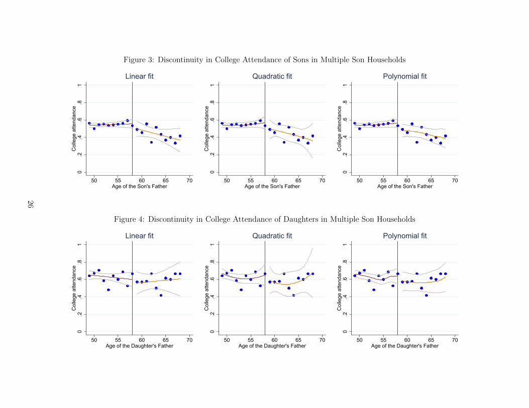
Figure 3: Discontinuity in College Attendance of Sons in Multiple Son Households

0.2

.4.6

.81

Col

lege

atte

ndan

ce

50 55 60 65 70Age of the Son's Father

Linear fit

0.2

.4.6

.81

Col

lege

atte

ndan

ce


Quadratic fit

0.2

.4.6

.81

Col

lege

atte

ndan

ce


Polynomial fit

Figure 4: Discontinuity in College Attendance of Daughters in Multiple Son Households

0.2

.4.6

.81

Col

lege

atte

ndan

ce

50 55 60 65 70Age of the Daughter's Father

Linear fit

0.2

.4.6

.81

Col

lege

atte

ndan

ce

50 55 60 65 70Age of the Daughter's Father

Quadratic fit

0.2

.4.6

.81

Col

lege

atte

ndan

ce50 55 60 65 70

Age of the Daughter's Father

Polynomial fit

26

Table 1: Types and Number of Households in the 2011 Census

Share out of allNumber Households with

head (in %)

All Households 423,637

without head 1,303

with head 422,334 100.0

but no spouse 68,341 16.2

and one spouse 353,001 83.6

and more than one spouse 992 0.2

Households with head living with

sons or daughter-in-laws of the head 6,312 1.5

parents of head or spouse 10,329 2.5

siblings of head or spouse 5,904 1.4

other relatives and non-relatives 2,542 0.6

Households with a mother and her husband 274,382 65.0

with all children present* 129,619 30.7

Sample of this study† 1,431 0.3

Note: This table contains the number of households in the census based on the

composition of the household. There are 1,481,586 individuals in the data.

Only 0.4 percent of them (5,840) are living in households without head. This study

only focuses on households that have a head and one spouse but do not have

any other member except children. These households may not have children at all.

* The households in this sample are identified using two rules: 1) The households

only consist of a male head, his spouse, and their children (no step-child,

another spouse, or any extended family member), 2) the number of father’s

children present in the household is equal to the number of children ever born by

the mother. Table 2 contains summary statistics of these mothers.† This is the sample of sole sons whose fathers age was between 49 and

68 when they were 18.

27

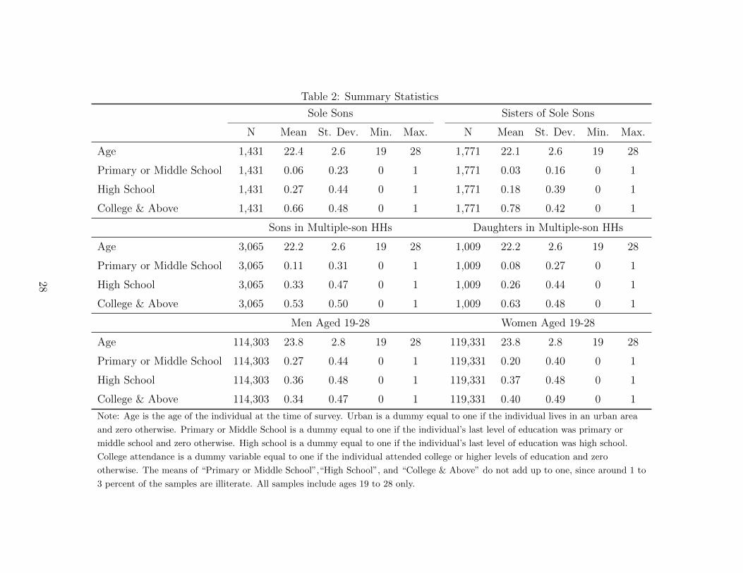
Table 2: Summary Statistics

Sole Sons Sisters of Sole Sons

N Mean St. Dev. Min. Max. N Mean St. Dev. Min. Max.

Age 1,431 22.4 2.6 19 28 1,771 22.1 2.6 19 28

Primary or Middle School 1,431 0.06 0.23 0 1 1,771 0.03 0.16 0 1

High School 1,431 0.27 0.44 0 1 1,771 0.18 0.39 0 1

College & Above 1,431 0.66 0.48 0 1 1,771 0.78 0.42 0 1

Sons in Multiple-son HHs Daughters in Multiple-son HHs

Age 3,065 22.2 2.6 19 28 1,009 22.2 2.6 19 28


High School 3,065 0.33 0.47 0 1 1,009 0.26 0.44 0 1

College & Above 3,065 0.53 0.50 0 1 1,009 0.63 0.48 0 1

Men Aged 19-28 Women Aged 19-28

Age 114,303 23.8 2.8 19 28 119,331 23.8 2.8 19 28


High School 114,303 0.36 0.48 0 1 119,331 0.37 0.48 0 1

College & Above 114,303 0.34 0.47 0 1 119,331 0.40 0.49 0 1

Note: Age is the age of the individual at the time of survey. Urban is a dummy equal to one if the individual lives in an urban area

and zero otherwise. Primary or Middle School is a dummy equal to one if the individual’s last level of education was primary or

middle school and zero otherwise. High school is a dummy equal to one if the individual’s last level of education was high school.

College attendance is a dummy variable equal to one if the individual attended college or higher levels of education and zero

otherwise. The means of “Primary or Middle School”,“High School”, and “College & Above” do not add up to one, since around 1 to

3 percent of the samples are illiterate. All samples include ages 19 to 28 only.

28

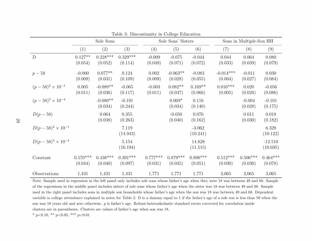
Table 3: Discontinuity in College Education

Sole Sons Sole Sons’ Sisters Sons in Multiple-Son HH

(1) (2) (3) (4) (5) (6) (7) (8) (9)

D 0.127** 0.228*** 0.329*** -0.009 -0.075 -0.044 0.044 0.064 0.080(0.054) (0.052) (0.114) (0.049) (0.071) (0.072) (0.033) (0.039) (0.079)

p− 58 -0.000 0.077** 0.124 0.002 -0.063** -0.083 -0.014*** -0.011 0.030(0.009) (0.031) (0.109) (0.009) (0.028) (0.055) (0.004) (0.027) (0.084)

(p− 58)2 × 10−1 0.005 -0.089** -0.065 -0.003 0.082** 0.169** 0.016*** 0.020 -0.056(0.011) (0.036) (0.117) (0.011) (0.037) (0.066) (0.005) (0.028) (0.086)

(p− 58)3 × 10−4 -0.080** -0.191 0.069* 0.116 -0.004 -0.101(0.034) (0.244) (0.034) (0.140) (0.028) (0.175)

D(p− 58) 0.064 0.355 -0.050 0.076 0.011 0.018(0.038) (0.263) (0.040) (0.162) (0.030) (0.182)

D(p− 58)2 × 10−1 7.119 -3.062 6.328(14.943) (10.241) (10.122)

D(p− 58)3 × 10−4 5.154 14.828 -12.510(16.194) (11.515) (10.695)

Constant 0.570*** 0.438*** 0.391*** 0.777*** 0.879*** 0.898*** 0.512*** 0.506*** 0.464***(0.044) (0.040) (0.097) (0.031) (0.035) (0.051) (0.030) (0.030) (0.078)

Observations 1,431 1,431 1,431 1,771 1,771 1,771 3,065 3,065 3,065

Note: Sample used in regression in the left panel only includes sole sons whose father’s age when they were 18 was between 49 and 68. Sample

of the regressions in the middle panel includes sisters of sole sons whose father’s age when the sister was 18 was between 49 and 68. Sample

used in the right panel includes sons in multiple son households whose father’s age when the son was 18 was between 49 and 68. Dependent

variable is college attendance explained in notes for Table 2. D is a dummy equal to 1 if the father’s age of a sole son is less than 59 when the

son was 18 years old and zero otherwise. p is father’s age. Robust-heteroskedastic standard errors corrected for correlation inside

clusters are in parentheses. Clusters are values of father’s age when son was 18.

* p<0.10, ** p<0.05, *** p<0.01

29

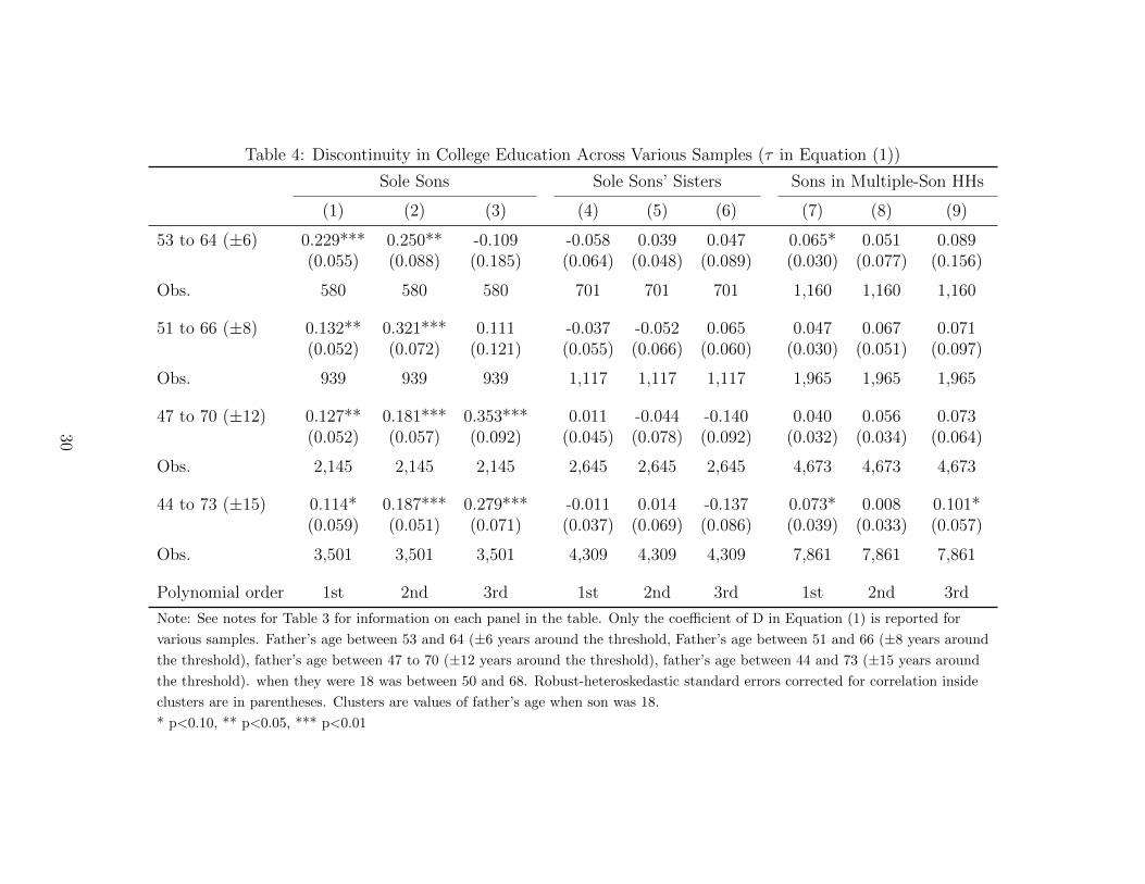
Table 4: Discontinuity in College Education Across Various Samples (τ in Equation (1))

Sole Sons Sole Sons’ Sisters Sons in Multiple-Son HHs

(1) (2) (3) (4) (5) (6) (7) (8) (9)

53 to 64 (±6) 0.229*** 0.250** -0.109 -0.058 0.039 0.047 0.065* 0.051 0.089(0.055) (0.088) (0.185) (0.064) (0.048) (0.089) (0.030) (0.077) (0.156)

Obs. 580 580 580 701 701 701 1,160 1,160 1,160

51 to 66 (±8) 0.132** 0.321*** 0.111 -0.037 -0.052 0.065 0.047 0.067 0.071(0.052) (0.072) (0.121) (0.055) (0.066) (0.060) (0.030) (0.051) (0.097)

Obs. 939 939 939 1,117 1,117 1,117 1,965 1,965 1,965

47 to 70 (±12) 0.127** 0.181*** 0.353*** 0.011 -0.044 -0.140 0.040 0.056 0.073(0.052) (0.057) (0.092) (0.045) (0.078) (0.092) (0.032) (0.034) (0.064)

Obs. 2,145 2,145 2,145 2,645 2,645 2,645 4,673 4,673 4,673

44 to 73 (±15) 0.114* 0.187*** 0.279*** -0.011 0.014 -0.137 0.073* 0.008 0.101*(0.059) (0.051) (0.071) (0.037) (0.069) (0.086) (0.039) (0.033) (0.057)

Obs. 3,501 3,501 3,501 4,309 4,309 4,309 7,861 7,861 7,861

Polynomial order 1st 2nd 3rd 1st 2nd 3rd 1st 2nd 3rd

Note: See notes for Table 3 for information on each panel in the table. Only the coefficient of D in Equation (1) is reported for

various samples. Father’s age between 53 and 64 (±6 years around the threshold, Father’s age between 51 and 66 (±8 years around

the threshold), father’s age between 47 to 70 (±12 years around the threshold), father’s age between 44 and 73 (±15 years around

the threshold). when they were 18 was between 50 and 68. Robust-heteroskedastic standard errors corrected for correlation inside

clusters are in parentheses. Clusters are values of father’s age when son was 18.

* p<0.10, ** p<0.05, *** p<0.01

30

Table 5: Discontinuity in College Attendance of Sole Sons (τ in Equation (2))

Sample I Sample II Sample III

(1) (2) (3) (4) (5) (6) (7) (8) (9)

D × S 0.136* 0.303*** 0.372** 0.118* 0.232*** 0.341** 0.107* 0.225*** 0.307**(0.076) (0.091) (0.147) (0.059) (0.056) (0.130) (0.058) (0.056) (0.122)

Polynomial order 1st 2nd 3rd 1st 2nd 3rd 1st 2nd 3rd

Observations 3,202 3,202 3,202 6,267 6,267 6,267 7,276 7,276 7,276

Note: Regressions are based on Equation (2). See notes for Table 3 for more information on variables. Coefficient of D × S shows

the Neighborhood Average Treatment Effect from a Diff-in-Disc regression. Sample I includes sole sons and sisters of sole sons.

Sample II adds sons in multiple-son households to Sample I. Sample III adds daughters in multiple-son households to Sample II.

Robust-heteroskedastic corrected for correlation inside clusters are in parentheses. Clusters are father’s age of the individual when

s/he was 18.

* p<0.10, ** p<0.05, *** p<0.01

31

Table 6: OLS and IV Estimates of Return to College Education on Job Status and Wages

Job Status ln(AW) OLS HEIS†

OLS IV OLS IV ln(W) ln(AW)(1) (2) (3) (4) (5) (6)

College & above 1.009*** 1.633*** 0.233*** 0.375*** 0.281*** 0.252***(0.088) (0.315) (0.021) (0.084) (0.038) (0.010)

Age -0.039 -0.041 0.141 -0.015(0.044) (0.048) (0.107) (0.016)

Age2 × 10−2 0.096 0.080 -0.001 0.000(0.096) (0.103) (0.002) (0.000)

Constant 1.954*** 1.802*** 13.571*** 13.663*** 10.480*** 13.272***(0.024) (0.083) (0.494) (0.570) (1.287) (0.191)

F-statistic† 2.658 2.466Observations 774 774 774 774 2,978 3,387Adj. R-squared 0.227 0.140 0.242 0.177 0.100 0.358

Note: Job Status is a variable that is one if the individual is an unskilled worker, two for semi-technical

workers, three for technicians and associate professionals, four for scientists, doctors, lawyers, and engineers,

and five for managers, and top government officials. ln(AW) is the natural log of the average wage for the

job status an individual has. ln(W) is the natural log of individual’s wage. IV estimates are 2SLS estimates

with Equation (2) as the first stage and the discontinuity as an instrument for college education. Robust-

heteroskedastic standard errors in parentheses.† OLS estimates using HEIS 2010 is the Household Expenditure and Income Survey of 2010.

* p<0.10, ** p<0.05, *** p<0.01

32

Sir! I’d Rather Go to School, Sir!

Documents