Singularly Perturbed Monotone Systems and an Application to Double Phosphorylation Cycles

arX

iv:m

ath/

0701

575v

2 [

mat

h.D

S] 7

Mar

200

7

Singularly Perturbed Monotone Systems and an Application to Double

Phosphorylation Cycles

Liming Wang and Eduardo Sontag∗†

February 2, 2008

Abstract

The theory of monotone dynamical systems has been found very useful in the modeling of somegene, protein, and signaling networks. In monotone systems, every net feedback loop is positive. Onthe other hand, negative feedback loops are important features of many systems, since they are requiredfor adaptation and precision. This paper shows that, provided that these negative loops act at acomparatively fast time scale, the main dynamical property of (strongly) monotone systems, convergenceto steady states, is still valid. An application is worked out to a double-phosphorylation “futile cycle”motif which plays a central role in eukaryotic cell signaling.

1 Introduction

Monotone dynamical systems constitute a rich class of models, for which global and almost-global con-vergence properties can be established. They are particularly useful in biochemical applications and alsoappear in areas like coordination [28] and other problems in control [7]. One of the fundamental resultsin monotone systems theory is Hirsch’s Generic Convergence Theorem [17, 18, 19, 37]. Informally stated,Hirsch’s result says that almost every bounded solution of a strongly monotone system converges to theset of equilibria. There is a rich literature regarding the application of this powerful theorem, as well asof other results dealing with everywhere convergence when equilibria are unique ([9, 22, 37]), to models ofbiochemical systems. See for instance [39, 40] for expositions and many references.

Unfortunately, many models in biology are not monotone, at least with respect to any standard orthantorder. This is because in monotone systems (with respect to orthant orders) every net feedback loop shouldbe positive, but, on the other hand, in many systems negative feedback loops often appear as well, as theyare required for adaptation and precision. However, intuitively, negative loops that act at a comparativelyfast time scale should not affect the main characteristics of monotone behavior. The main purpose of thispaper is to show that this is indeed the case, in the sense that singularly perturbed strongly monotonesystems inherit generic convergence properties. A system that is not monotone may become monotone oncethat fast variables are replaced by their steady-state values. In order to prove a precise time-separationresult, we employ tools from geometric singular perturbation theory.

This point of view is of special interest in the context of biochemical systems; for example, MichaelisMenten kinetics are mathematically justified as singularly perturbed versions of mass action kinetics [11,29]. One particular example of great interest in view of current systems biology research is that of “futilecycle” motifs, as illustrated in Figure 1. As discussed in [34], futile cycles (with any number of intermediate

∗L. Wang is with the Rutgers University, Department of Mathematics, [email protected].†E. Sontag is with the Rutgers University, Department of Mathematics, [email protected].

1

F

E

F

E

S S0 2S1

Figure 1: Dual futile cycle. A substrate S0 is ultimately converted into a product P , in an “activation”reaction triggered or facilitated by an enzyme E, and, conversely, P is transformed back (or “deactivated”)into the original S0, helped on by the action of a second enzyme F .

steps, and also called substrate cycles, enzymatic cycles, or enzymatic interconversions) underlie signal-ing processes such as GTPase cycles [10], bacterial two-component systems and phosphorelays [3, 15] actintreadmilling [6]), and glucose mobilization [24], as well as metabolic control [41] and cell division and apop-tosis [42] and cell-cycle checkpoint control [26]. A most important instance is that of Mitogen-ActivatedProtein Kinase (“MAPK”) cascades, which regulate primary cellular activities such as proliferation, differ-entiation, and apoptosis [2, 5, 20, 46] in eukaryotes from yeast to humans. MAPK cascades usually consistof three tiers of similar structures with multiple feedbacks [4], [13], [47]. Here we focus on one individuallevel of a MAPK cascade, which is a futile cycle as depicted in Figure 1. The precise mathematical model isdescribed later. Numerical simulations of this model have suggested that the system may be monostable orbistable, see [27]. The later will give rise to switch-like behavior, which is ubiquitous in cellular pathways([14, 32, 35, 36]). In either case, the system under meaningful biological parameters shows convergence,not other dynamical properties such as periodic behavior or even chaotic behavior. Analytical studies donefor the quasi-steady-state version of the model (slow dynamics), which is a monotone system, indicate thatthe reduced system is indeed monostable or bistable, see [31]. Thus, it is of great interest to show that,at least in certain parameter ranges (as required by singular perturbation theory), the full system inheritsconvergence properties from the reduced system, and this is what we do as an application of our results.

A feature of our approach, as in other control problems [1], [21], is the use of geometric invariantmanifold theory [12, 23, 30]. There is a manifold Mε, invariant for the full dynamics of a singularlyperturbed system, which attracts all near-enough solutions. However, we need to exploit the full power ofthe theory, and especially the fibration structure and an asymptotic phase property. The system restrictedto the invariant manifold Mε is a regular perturbation of the slow (ε=0) system. As remarked in Theorem1.2 in Hirsch’s early paper [17], a C1 regular perturbation of a flow with eventually positive derivativesalso has generic convergence properties. So, solutions in the manifold will generally be well-behaved, andasymptotic phase implies that solutions nearMε track solutions inMε, and hence also converge to equilibriaif solutions on Mε do. A key technical detail is to establish that the tracking solutions also start from the“good” set of initial conditions, for generic solutions of the large system.

A preliminary version of these results was presented at the 2006 Conference on Decision and Control,and dealt with the special case of singularly perturbed systems of the form:

x =f(x, y)

εy =Ay + h(x)

on a product domain, where A is a constant Hurwitz matrix and the reduced system x = f(x,−A−1h(x))is strongly monotone. However, for the application to the above futile cycle, there are two major problemswith that formulation: first, the dynamics of the fast system have to be allowed to be nonlinear in y, andsecond, it is crucial to allow for an ε-dependence on the right-hand side as well as to allow the domain tobe a polytope depending on ε. We provide a much more general formulation here.

We note that no assumptions are imposed regarding global convergence of the reduced system, which

2

is essential because of the intended application to multi-stable systems. This seems to rule out the appli-cability of Lyapunov-theoretic and ISS tools [8, 43].

This paper is organized as follows. The main result is stated in Section 2. In Section 3, we reviewsome basic definitions and theorems about monotone systems. The detailed proof of the main theoremcan be found in Section 4, and applications to the MAPK system and another set of ordinary differentialequations are discussed in Section 5. Finally, in Section 6, we summarize the key points of this paper.

2 Statement of the Main Theorem

In this paper, we focus on the dynamics of the following prototypical system in singularly perturbed form:

dx

dt= f0(x, y, ε) (1)

εdy

dt= g0(x, y, ε).

We will be interested in the dynamics of this system on a time-varying domain Dε. For 0 < ε ≪ 1, thevariable x changes much slower than y. As long as ε 6= 0, one may also change the time scale to τ = t/ε,and study the equivalent form:

dx

dτ= εf0(x, y, ε) (2)

dy

dτ= g0(x, y, ε).

Within this general framework, we will make the following assumptions (some technical terms will bedefined later), where the integer r > 1 and the positive number ε0 are fixed from now on:

A1 Let U ⊂ Rn and V ⊂ R

m be open and bounded. The functions

f0 : U × V × [0, ε0] → Rn

g0 : U × V × [0, ε0] → Rm

are both of class Crb , where a function f is in Cr

b if it is in Cr and its derivatives up to order r aswell as f itself are bounded.

A2 There is a functionm0 : U → V

of class Crb , such that g0(x,m0(x), 0) = 0 for all x in U .

It is often helpful to consider z = y −m0(x), and the fast system (2) in the new coordinates becomes:

dx

dτ= εf1(x, z, ε) (3)

dz

dτ= g1(x, z, ε),

3

where

f1(x, z, ε) = f0(x, z +m0(x), ε),

g1(x, z, ε) = g0(x, z +m0(x), ε) − ε[Dxm0(x)]f1(x, z, ε).

When ε = 0, the system (3) degenerates to

dz

dτ= g1(x, z, 0), x(τ) ≡ x0 ∈ U, (4)

seen as equations on z | z +m0(x0) ∈ V .

A3 The steady state z = 0 of (4) is globally asymptotically stable on z | z +m0(x0) ∈ V for all x0 ∈ U .

A4 All eigenvalues of the matrix Dyg0(x,m0(x), 0) have negative real parts for every x ∈ U , i.e. thematrix Dyg0(x,m0(x), 0) is Hurwitz on U .

A5 There exists a family of convex compact sets Dε ⊂ U × V , which depend continuously on ε ∈ [0, ε0],such that (1) is positively invariant on Dε for ε ∈ (0, ε0].

A6 The flow ψ0t of the limiting system (set ε = 0 in (1)):

dx

dt= f0(x,m0(x), 0) (5)

has eventually positive derivatives on K0, where K0 is the projection of

D0

⋂

(x, y) | y = m0(x), x ∈ U

onto the x-axis.

A7 The set of equilibria of (1) on Dε is totally disconnected.

Remark 1 Assumption A3 implies that y = m0(x) is a unique solution of g0(x, y, 0) = 0 on U .

Continuity in A5 is understood with respect to the Hausdorff metric.

In mass-action chemical kinetics, the vector fields are polynomials. So, A1 follows naturally.

Our main theorem is:

Theorem 1 Under assumptions A1 to A7, there exists a positive constant ε∗ < ε0 such that for each ε ∈(0, ε∗), the forward trajectory of (1) starting from almost every point in Dε converges to some equilibrium.

3 Monotone Systems of Ordinary Differential Equations

In this section, we review several useful definitions and theorems regarding monotone systems. As wewish to provide results valid for arbitrary orders, not merely orthants, and some of these results, thoughwell-known, are not readily available in a form needed for reference, we provide some technical proofs.

Definition 1 A nonempty, closed set C ⊂ RN is a cone if

4

1. C + C ⊂ C,

2. R+C ⊂ C,

3. C⋂

(−C) = 0.

We always assume C 6= 0. Associated to a cone C is a partial order on RN . For any x, y ∈ R

N , wedefine:

x ≥ y ⇔ x− y ∈ C

x > y ⇔ x− y ∈ C, x 6= y.

When IntC is not empty, we can define

x≫ y ⇔ x− y ∈ IntC.

Definition 2 The dual cone of C is defined as

C∗ = λ ∈ (RN )∗ |λ(C) ≥ 0.

An immediate consequence is

x ∈ C ⇔ λ(x) ≥ 0,∀λ ∈ C∗

x ∈ IntC ⇔ λ(x) > 0,∀λ ∈ C∗ \ 0.

With this partial ordering on RN , we analyze certain features of the dynamics of an ordinary differential

equation:

dz

dt= F (z), (6)

where F : RN → R

N is a C1 vector field. We are interested in a special class of equations which preservethe ordering along the trajectories. For simplicity, the solutions of (6) are assumed to exist for all t ≥ 0 inthe sets considered below.

Definition 3 The flow φt of (6) is said to have (eventually) positive derivatives on a set V ⊆ RN , if

[Dzφt(z)]x ∈ IntC for all x ∈ C \ 0, z ∈ V , and t ≥ 0 (t ≥ t0 for some t0 > 0).

It is worth noticing that [Dzφt(z)]x ∈ IntC is equivalent to λ([Dzφt(z)]x) > 0 for all λ ∈ C∗ with normone. We will use this fact in the proof of the next lemma, which deals with “regular” perturbations in thedynamics. The proof is in the same spirit as in Theorem 1.2 of [18], but generalized to the arbitrary coneC.

Lemma 1 Assume V ⊂ RN is a compact set in which the flow φt of (6) has eventually positive derivatives.

Then there exists δ > 0 with the following property. Let ψt denote the flow of a C1 vector field G such thatthe C1 norm of F (z) −G(z) is less than δ for all z in V . Then there exists t∗ > 0 such that if ψs(z) ∈ Vfor all s ∈ [0, t] where t ≥ t∗, then [Dzψt(z)]x ∈ IntC for all z ∈ V and x ∈ C \ 0.

5

Proof. Pick t0 > 0 so that λ([Dzφt(z)]x) > 0 for all t ≥ t0, z ∈ V, λ ∈ C∗, x ∈ C with |λ| = 1, |x| = 1.Then there exists δ > 0 with the property that when the C1 norm of F (z) −G(z) is less than δ, we haveλ([Dzψt(z)]x) > 0 for t0 ≤ t ≤ 2t0.

When t > 2t0, we write t = r + kt0, where t0 ≤ r < 2t0 and k ∈ N. If ψs(z) ∈ V for all s ∈ [0, t], wecan define zj := ψjt0(z) for j = 0, . . . , k. For any x ∈ C \ 0, using the chain rule, we have:

[Dzψt(z)]x = [Dzψr(zk)][Dzψt0(zk−1)] · · · [Dzψt0(z0)]x.

By induction, it is easy to see that [Dzψt(z)]x ∈ IntC.

Corollary 1 If V is positively invariant under the flow ψt, then ψt has eventually positive derivatives inV .

Proof. If V is positively invariant under the flow ψt, then for any z ∈ V the condition ψs(z) ∈ V fors ∈ [0, t] is satisfied for all t ≥ 0. By the previous lemma, ψt has eventually positive derivatives in V .

Definition 4 The system (6) or the flow φt of (6) is called monotone (resp. strongly monotone) in a setW ⊆ R

N , if for all t ≥ 0 and z1, z2 ∈W ,

z1 ≥ z2 ⇒φt(z1) ≥ φt(z2)

(resp. φt(z1) ≫ φt(z2) when z1 6= z2).

It is eventually (strongly) monotone if there exists t0 ≥ 0 such that φt is (strongly) monotone for all t ≥ t0.

Definition 5 An set W ⊆ RN is called p-convex, if W contains the entire line segment joining x and y

whenever x ≤ y, x, y ∈W .

The next two propositions discuss the relations between the two definitions, (eventually) positive derivativesand (eventually) strongly monotone.

Proposition 1 Let W ⊆ RN be p-convex. If the flow φt has (eventually) positive derivatives in W , then

it is (eventually) strongly monotone in W .

Proof. For any z1 > z2 ∈W,λ ∈ C∗\0 and t ≥ 0 (t ≥ t0 for some t0 > 0), we have that λ(φt(z1)−φt(z2))equals

∫ 1

0λ(

[Dzφt(sz1 + (1 − s)z2)](z1 − z2))

ds > 0.

Therefore, φt is (eventually) strongly monotone in W .

Proposition 2 Suppose φt is (eventually) strongly monotone on an open set U ⊆ RN . Then φt has

(eventually) positive derivatives in U .

Proof. Fix t > 0 such that φt as a function from U to RN is strongly monotone (i.e. φt(z1) ≫ φt(z2),

whenever z1 ≥ z2, z1 6= z2 in U).

For any λ ∈ C∗ \ 0, x ∈ C \ 0, and z ∈ U ,

λ([Dzφt(z)]x) = limh→0

h−1λ(φt(z + hx) − φt(z)).

If h > 0 is small enough such that z+hx ∈ U , then we have λ(

φt(z+hx)−φt(z))

> 0. Thus λ([Dzφt(z)]x) >0, and [Dzφt(z)]x ∈ IntC.

6

Lemma 2 Suppose that the flow φt of (6) has compact closure and eventually positive derivatives in ap-convex set W ⊆ R

N . If the set of equilibria is totally disconnected (e.g. countable), then the forwardtrajectory starting from almost every point in W converges to an equilibrium.

Proof. By Proposition 1, φt is eventually strongly monotone. The result easily follows from Hirsch’sGeneric Convergence Theorem ([19], [37]).

4 Details of the Proof

Our approach to solve the varying domain problem is motivated by Nipp [30]. The idea is to extend thevector field from U × V × [0, ε] to Rn × Rm × [0, ε0], then apply geometric singular perturbation theorems([33]) on R

n × Rm × [0, ε0], and finally restrict the flows to Dε for the generic convergence result.

4.1 Extensions of the vector field

For a given compact set K ⊂ Rn (K0 ⊆ K ⊂ U), the following procedure is adopted from [30] to extend

a Crb function with respect to the x coordinate from U to R

n, such that the extended function is Crb and

agrees with the old one on K. This is a routine “smooth patching” argument.

Let U1 be an open subset of U with Cr boundary and such that K ⊂ U1 ⊆ U . For Θ0 > 0 sufficientlysmall, define

UΘ0

1 := x ∈ U1 |Θ(x) ≥ Θ0, where Θ(x) := minu∈∂U1

|x− u|,

such that K is contained in UΘ0

1 . Consider the scalar C∞ function ρ:

ρ(a) :=

0 a ≤ 0exp(1 − exp(a− 1)/a) 0 < a < 11 a ≥ 1.

Define

Θ(x) :=

0 x ∈ Rn \ U1

Θ(x) x ∈ U1 \ UΘ0

1

Θ0 x ∈ UΘ0

1 ,

and

Θ(x) := ρ(Θ(x)

Θ0

)

.

For any q ∈ Crb (U), let

¯q(x) :=

q(x) x ∈ U1

0 x ∈ Rn \ U1,

and q(x) := Θ(x)¯q(x).

Then q(x) ∈ Crb (Rn) and q(x) ≡ q(x) on K.

We fix some d0 > 0 such that

Dd0:= z ∈ R

m | |z| ≤ d0 ⊂⋂

x∈K

z | z +m0(x) ∈ V .

7

Then we extend the functions f1 and m0 to f1 and m0 respectively with respect to x in the above way. Toextend g1, let us first rewrite the differential equation for z as:

dz

dτ=[B(x) + C(x, z)]z + εH(x, z, ε) − ε[Dxm0(x)]f1(x, z, ε),

whereB(x) = Dyg0(x,m0(x), 0) and C(x, 0) = 0.

Following the above procedures, we extend the functions C and H to C and H, but the extension of B isdefined as

B(x) := Θ(x) ¯B(x) − µ(1 − Θ(x))In,

where µ is the positive constant such that the real parts of all eigenvalues of B(x) is less than −µ for everyx ∈ K. According to the definition of B(x), all eigenvalues of B(x) will have negative real parts less than−µ for every x ∈ R

n. The extension g1, defined as:

[B(x) + C(x, z)]z + εH(x, z, ε) − ε[Dxm0(x)]f1(x, z, ε),

is then Cr−1b (Rn ×Dd0

× [0, ε0]) and agrees with g1 on K ×Dd0× [0, ε0].

To extend functions f1 and g1 in the z direction from Dd0to R

m, we use the same extension techniquebut with respect to z. Let us denote the extensions of f1, C, H and the function z = z by f1, C, H and zrespectively, then define g1 as:

[B(x) + C(x, z)]z(z) + εH(x, z, ε) − ε[Dxm0(x)]f1(x, z, ε),

which is now Cr−1b (Rn ×R

m × [0, ε0]) and agrees with g1 on K ×Dd1× [0, ε0] for some d1 slightly less than

d0. Notice that z = 0 is a solution of g1(x, z, 0) = 0, which guarantees that for the extended system in(x, y) coordinates (y = z + m0(x)):

dx

dτ= εf(x, y, ε) (7)

dy

dτ= g(x, y, ε),

y = m0(x) is the solution of g(x, y, 0) = 0. To summarize, (7) satisfies

E1 The functionsf ∈ Cr

b (Rn × Rm × [0, ε0]),

g ∈ Cr−1b (Rn × R

m × [0, ε0]),

m0 ∈ Crb (Rn), g(x, m0(x), 0) = 0, ∀x ∈ R

n.

E2 All eigenvalues of the matrix Dyg(x, m0(x), 0) have negative real parts less than −µ for every x ∈ Rn.

E3 The function m0 coincides with m0 on K, and the functions f and g coincide with f0 and g0 respectivelyon

Ωd1:= (x, y) |x ∈ K, |y −m0(x)| ≤ d1.

Conditions E1 and E2 are the assumptions for geometric singular perturbation theorems, and conditionE3 ensures that on Ωd1

the flow of (2) coincides with the flow of (7). If we apply geometric singularperturbation theorems to (7) on R

n × Rm × [0, ε0], the exact same results are true for (2) on Ωd1

. For therest of the paper, we identify the flow of (7) and the flow of (2) on Ωd1

without further mentioning thisfact.(Later, in Lemmas 4-7, when globalizing the results, we consider again the original system.)

8

4.2 Geometric singular perturbation theory

The theory of geometric singular perturbation can be traced back to the work of Fenichel [12], which firstrevealed the geometric aspects of singular perturbation problems. Later on, the works by Knobloch andAulbach [25], Nipp [30], and Sakamoto [33] also presented results similar to [12]. By now, the theoryis fairly standard, and there have been enormous applications to traveling waves of partial differentialequations, see [23] and the references there. For control theoretic applications, see [1, 21].

To apply geometric singular perturbation theorems to the vector field on Rn × R

m × [0, ε0], we use thetheorems stated in [33]. The following lemma is a restatement of the theorems in [33], and we refer to [33]for the proof.

Lemma 3 Under conditions E1 and E2, there exists a positive ε1 < ε0 such that for every ε ∈ (0, ε1]:

1. There is a Cr−1b function

m : Rn × [0, ε1] → R

m

such that the set Mε defined by

Mε := (

x,m(x, ε))

|x ∈ Rn

is invariant under the flow generated by (7). Moreover,

supx∈Rn

|m(x, ε) − m0(x)| = O(ε), as ε→ 0.

In particular, we have m(x, 0) = m0(x) for all x ∈ Rn.

2. The set consisting of all the points (x0, y0) such that

supτ≥0

|y(τ ;x0, y0) −m(

x(τ ;x0, y0), ε)

|eµτ

4 <∞,

where(

x(τ ;x0, y0), y(τ ;x0, y0))

is the solution of (7) passing through (x0, y0) at τ = 0, is a Cr−1-immersed submanifold in R

n × Rm of dimension n+m, denoted by W s(Mε).

3. There is a positive constant δ0 such that if

supτ≥0

|y(τ ;x0, y0) −m(

x(τ ;x0, y0), ε)

| < δ0,

then (x0, y0) ∈W s(Mε).

4. The manifold W s(Mε) is a disjoint union of Cr−1-immersed manifolds W sε (ξ) of dimension m:

W s(Mε) =⋃

ξ∈Rn

W sε (ξ).

For each ξ ∈ Rn, let Hε(ξ)(τ) be the solution for τ ≥ 0 of

dx

dτ= εf(x,m(x, ε), ε), x(0) = ξ ∈ R

n.

Then, the manifold W sε (ξ) is the set

(x0, y0) | supτ≥0

|x(τ)|eµτ

4 <∞, supτ≥0

|y(τ)|eµτ

4 <∞,

9

where

x(τ) = x(τ ;x0, y0) −Hε(ξ)(τ),

y(τ) = y(τ ;x0, y0) −m(

Hε(ξ)(τ), ε)

.

5. The fibers are “positively invariant” in the sense that W sε (Hε(ξ)(τ)) is the set

(

x(τ ;x0, y0), y(τ ;x0, y0))

| (x0, y0) ∈W sε (ξ)

for each τ ≥ 0, see Figure 2.

6. The fibers restricted to the δ0 neighborhood of Mε, denoted by W sε,δ0

, can be parametrized as follows.

There are two Cr−1b functions

Pε,δ0 : Rn ×Dδ0 → R

n

Qε,δ0 : Rm ×Dδ0 → R

m,

and a mapTε,δ0 : R

n ×Dδ0 → Rn × R

m

mapping (ξ, η) to (x, y), where

x = ξ + Pε,δ0(ξ, η), y = m(x, ε) +Qε,δ0(ξ, η)

such thatW s

ε,δ0(ξ) = Tε,δ0(ξ,Dδ0).

Remark 2 The δ0 in property 3 can be chosen uniformly for ε ∈ (0, ε0]. Without loss of generality, weassume that δ0 < d1.

Notice that property 4 insures that for each (x0, y0) ∈W s(Mε), there exists a ξ such that

|x(τ ;x0, y0) −Hε(ξ)(τ)| → 0,

|y(τ ;x0, y0) −m(

Hε(ξ)(τ), ε)

| → 0.

as t→ 0. This is often referred as the “asymptotic phase” property, see Figure 2.

4.3 Further analysis of the dynamics

The first property of Lemma 3 concludes the existence of an invariant manifold Mε. There are two reasonsto introduce Mε. First, on Mε the x-equation is decoupled from the y-equation:

dx

dt= f(x,m(x, ε), ε) (8)

y(t) = m(x(t), ε).

This reduction allows us to analyze a lower dimensional system, whose dynamics may have been wellstudied. Second, when ε approaches zero, the limit of (8) is (5) on K0. If (5) has some desirable property,it is natural to expect that this property is inherited by (8). An example of this principle is provided bythe following Lemma:

10

Mε

qqq

pp

01

1

22

0p

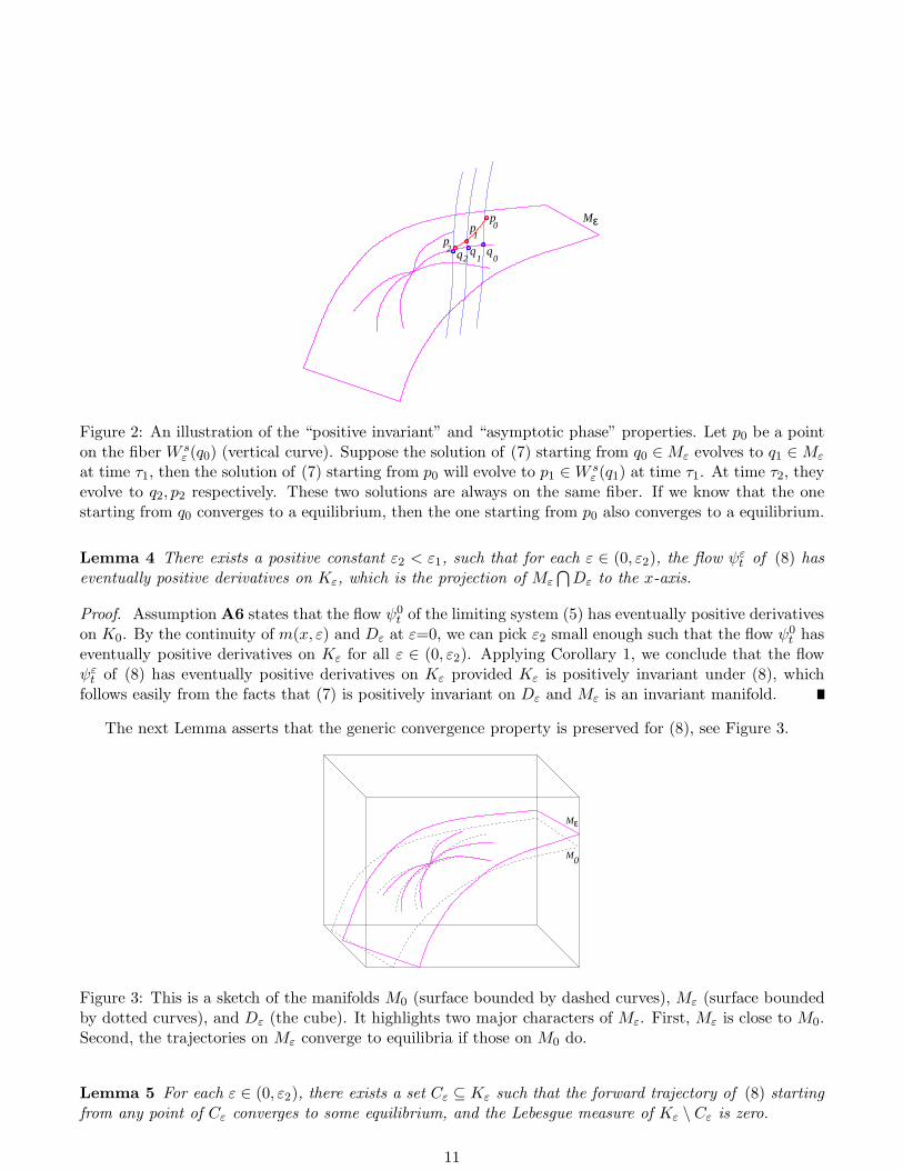
Figure 2: An illustration of the “positive invariant” and “asymptotic phase” properties. Let p0 be a pointon the fiber W s

ε (q0) (vertical curve). Suppose the solution of (7) starting from q0 ∈Mε evolves to q1 ∈Mε

at time τ1, then the solution of (7) starting from p0 will evolve to p1 ∈W sε (q1) at time τ1. At time τ2, they

evolve to q2, p2 respectively. These two solutions are always on the same fiber. If we know that the onestarting from q0 converges to a equilibrium, then the one starting from p0 also converges to a equilibrium.

Lemma 4 There exists a positive constant ε2 < ε1, such that for each ε ∈ (0, ε2), the flow ψεt of (8) has

eventually positive derivatives on Kε, which is the projection of Mε

⋂

Dε to the x-axis.

Proof. Assumption A6 states that the flow ψ0t of the limiting system (5) has eventually positive derivatives

on K0. By the continuity of m(x, ε) and Dε at ε=0, we can pick ε2 small enough such that the flow ψ0t has

eventually positive derivatives on Kε for all ε ∈ (0, ε2). Applying Corollary 1, we conclude that the flowψε

t of (8) has eventually positive derivatives on Kε provided Kε is positively invariant under (8), whichfollows easily from the facts that (7) is positively invariant on Dε and Mε is an invariant manifold.

The next Lemma asserts that the generic convergence property is preserved for (8), see Figure 3.

M

Mε

0

Figure 3: This is a sketch of the manifolds M0 (surface bounded by dashed curves), Mε (surface boundedby dotted curves), and Dε (the cube). It highlights two major characters of Mε. First, Mε is close to M0.Second, the trajectories on Mε converge to equilibria if those on M0 do.

Lemma 5 For each ε ∈ (0, ε2), there exists a set Cε ⊆ Kε such that the forward trajectory of (8) startingfrom any point of Cε converges to some equilibrium, and the Lebesgue measure of Kε \ Cε is zero.

11

Proof. Apply Lemma 2 and Lemma 4 under assumptions A5 and A7.

By now, we have discussed flows restricted to the invariant manifold Mε. Next, we will explore theconditions for a point to be on W s(Mε), the stable manifold of Mε. Property 3 of Lemma 3 provides asufficient condition, namely, any point (x0, y0) such that

supτ≥0

|y(τ ;x0, y0) −m(

x(τ ;x0, y0), ε)

| < δ0 (9)

is on W s(Mε). In fact, if we know that the difference between y0 and m(x0, ε) is sufficiently small, thenthe above condition is always satisfied. More precisely, we have:

Lemma 6 There exists ε3 > 0, δ0 > d > 0, such that for each ε ∈ (0, ε3), if the initial condition satisfies|y0 −m(x0, ε)| < d, then (9) holds, i.e. (x0, y0) ∈W s(Mε).

Proof. Follows from the proof of Claim 1 in [30].

Before we get further into the technical details, let us give an outline of the proof of the main theorem.The proof can be decomposed into three steps. First, we show that almost every trajectory on Dε

⋂

Mε

converges to some equilibrium. This is precisely Lemma 5. Second, we show that almost every trajectorystarting from W s(Mε) converges to some equilibrium. This follows from Lemma 5 and the “asymptoticphase” property in Lemma 3, but we still need to show that the set of non-convergent initial conditions isof measure zero. The last step is to show that all trajectories in Dε will eventually stay in W s(Mε), whichis our next lemma:

Lemma 7 There exist positive τ0 and ε4 < ε3, such that (x(τ0), y(τ0)) ∈W s(Mε) for all ε ∈ (0, ε4), where(x(τ), y(τ)) is the solution to (2) with the initial condition (x0, y0) ∈ Dε.

Proof. It is convenient to consider the problem in (x, z) coordinates. Let (x(τ), z(τ)) be the solution to(3) with initial condition (x0, z0), where z0 = y0 −m(x0, 0). We first show that there exists a τ0 such that|z(τ0)| ≤ d/2.

Expanding g1(x, z, ε) at the point (x0, z, 0), the equation of z becomes

dz

dτ= g1(x0, z, 0) +

∂g1∂x

(ξ, z, 0)(x − x0) + εR(x, z, ε)

for some ξ(τ) between x0 and x(τ) (where ξ(τ) can be picked continuously in τ). Let us write

z(τ) = z0(τ) + w(τ),

where z0(τ) is the solution to (4) with initial the condition z0(0) = z0, and w(τ) satisfies

dw

dτ= g1(x0, z, 0) − g1(x0, z

0, 0) +∂g1∂x

(ξ, z, 0)(x − x0) + εR(x, z, ε) (10)

=∂g1∂z

(x0, ζ, 0)w + ε∂g1∂x

(ξ, z, 0)

∫ τ

0f1(x(s), z(s), ε) ds + εR(x, z, ε),

with the initial condition w(0) = 0 and some ζ(τ) between z0(τ) and z(τ) (where ζ(τ) can be pickedcontinuously in τ).

By assumption A3, there exist a positive τ0 such that |z0(τ)| ≤ d/4 for all τ ≥ τ0. Notice that we areworking on the compact set Dε, so τ0 can be chosen uniformly for all initial conditions in Dε.

12

We write the solution of (10) as:

w(τ) =

∫ τ

0

∂g1∂z

(x0, ζ, 0)w ds+ ε

∫ τ

0

(∂g1∂x

(ξ, z, 0)

∫ s′

0f1(x, z, ε) ds

′ +R(x, z, ε))

ds.

Since the functions f1, R and the derivatives of g1 are bounded on Dε, we have:

|w(τ)| ≤

∫ τ

0L|w| ds + ε

∫ τ

0

(

M1

∫ s′

0M2 ds

′ +M3

)

ds,

for some positive constants L,Mi, i = 1, 2, 3. The notation |w| means the Euclidean norm of w ∈ Rm.

Moreover, if we define

α(τ) =

∫ τ

0

(

M1

∫ s′

0M2 ds

′ +M3

)

ds,

then

|w(τ)| ≤

∫ τ

0L|w| ds + εα(τ0),

for all τ ∈ [0, τ0] as α is increasing in τ . Applying Gronwall’s inequality ([38]), we have:

|w(τ)| ≤ εα(τ0)eLτ ,

which holds in particular at τ = τ0. Finally, we choose ε4 small enough such that εα(τ0)eLτ0 < d/4 and

|m(x, ε) −m(x, 0)| < d/2 for all ε ∈ (0, ε4). Then we have:

|y(τ0) −m(x(τ0), ε)| ≤ |y(τ0) −m(x(τ0), 0)| + |m(x(τ0), ε) −m(x(τ0), 0)|

< |z(τ0)| + d/2

< d/2 + d/2 = d.

That is, (x(τ0), y(τ0)) ∈W s(Mε) by Lemma 6.

By now, we have completed all these three steps, and are ready to prove Theorem 1.

4.4 Proof of Theorem 1

Proof. Let ε∗ = minε2, ε4. For ε ∈ (0, ε∗), it is equivalent to prove the result for the fast system (2).Pick an arbitrary point (x0, y0) in Dε, and there are three cases:

1. y0 = m(x0, ε), that is, (x0, y0) ∈ Mε

⋂

Dε. By Lemma 5, the forward trajectory converges to anequilibrium except for a set of measure zero.

2. 0 < |y0 − m(x0, ε)| < d. By Lemma 6, we know that (x0, y0) is in W s(Mε). Then, property 4 ofLemma 3 guarantees that the point (x0, y0) is on some fiber W s

ε,d(ξ), where ξ ∈ Kε. If ξ ∈ Cε, that is,the forward trajectory of ξ converges to some equilibrium, then by the “asymptotic phase” propertyof Lemma 3, the forward trajectory of (x0, y0) also converges to an equilibrium. To deal with thecase when ξ is not in Cε, it is enough to show that the set

Bε,d =⋃

ξ∈Kε\Cε

W sε,d(ξ)

13

has measure zero in Rm+n. Define

Sε,d = (Kε \ Cε) ×Dd.

By Lemma 5, Kε \Cε has measure zero in Rn, thus Sε,d has measure zero in R

n ×Rm. On the other

hand, property 6 in Lemma 3 implies Bε,d = Tε,d(Sε,d). Since Lipschitz maps send measure zero setsto measure zero sets, Bε,d is of measure zero.

3. |y0 −m(x0, ε)| ≥ d. By Lemma 7, the point(

x(τ0), y(τ0))

is in W s(Mε) and we are back to case 2.The proof is completed if the set φε

−τ0(Bε,d) has measure zero, where φε

τ is the flow of (2). This istrue because φε

τ is a diffeomorphism for any finite τ .

5 Applications

5.1 An application to the dual futile cycle

We assume that the reactions in Figure 1 follow the usual enzymatic mechanism ([13]):

S0 + Ek1−→←−k−1

C1k2→ S1 + E

k3−→←−k−3

C2k4→ S2 + E

S2 + Fh1−→←−h−1

C3h2→ S1 + F

h3−→←−h−3

C4h4→ S0 + F.

There are three conservation relations:

Stot = [S0] + [S1] + [S2] + [C1] + [C2] + [C4] + [C3],

Etot = [E] + [C1] + [C2],

Ftot = [F ] + [C4] + [C3],

where brackets indicate concentrations. Based on mass action kinetics, we have the following set of ordinarydifferential equations:

d[S0]

dτ= h4[C4] − k1[S0][E] + k−1[C1]

d[S2]

dτ= k4[C2] − h1[S2][F ] + h−1[C3]

d[C1]

dτ= k1[S0][E] − (k−1 + k2)[C1] (11)

d[C2]

dτ= k3[S1][E] − (k−3 + k4)[C2]

d[C4]

dτ= h3[S1][F ] − (h−3 + h4)[C4]

d[C3]

dτ= h1[S2][F ] − (h−1 + h2)[C3].

14

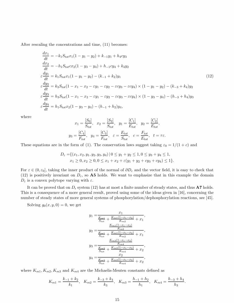
After rescaling the concentrations and time, (11) becomes:

dx1

dt= −k1Stotx1(1 − y1 − y2) + k−1y1 + h4cy3

dx2

dt= −h1Stotcx2(1 − y3 − y4) + h−1cy4 + k4y2

εdy1

dt= k1Stotx1(1 − y1 − y2) − (k−1 + k2)y1 (12)

εdy2

dt= k3Stot(1 − x1 − x2 − εy1 − εy2 − εcy3 − εcy4) × (1 − y1 − y2) − (k−3 + k4)y2

εdy3

dt= h3Stot(1 − x1 − x2 − εy1 − εy2 − εcy3 − εcy4) × (1 − y3 − y4) − (h−3 + h4)y3

εdy4

dt= h1Stotx2(1 − y3 − y4) − (h−1 + h2)y4,

where

x1 =[S0]

Stot, x2 =

[S2]

Stot, y1 =

[C1]

Etot, y2 =

[C2]

Etot,

y3 =[C4]

Ftot, y4 =

[C3]

Ftot, ε =

Etot

Stot, c =

Ftot

Etot, t = τε.

These equations are in the form of (1). The conservation laws suggest taking ε0 = 1/(1 + c) and

Dε =(x1, x2, y1, y2, y3, y4) | 0 ≤ y1 + y2 ≤ 1, 0 ≤ y3 + y4 ≤ 1,

x1 ≥ 0, x2 ≥ 0, 0 ≤ x1 + x2 + ε(y1 + y2 + cy3 + cy4) ≤ 1.

For ε ∈ (0, ε0], taking the inner product of the normal of ∂Dε and the vector field, it is easy to check that(12) is positively invariant on Dε, so A5 holds. We want to emphasize that in this example the domainDε is a convex polytope varying with ε.

It can be proved that on Dǫ system (12) has at most a finite number of steady states, and thus A7 holds.This is a consequence of a more general result, proved using some of the ideas given in [16], concerning thenumber of steady states of more general systems of phosphorylation/dephosphorylation reactions, see [45].

Solving g0(x, y, 0) = 0, we get

y1 =x1

Km1

Stot+ Km1(1−x1−x2)

Km2+ x1

,

y2 =

Km1(1−x1−x2)Km2

Km1

Stot+ Km1(1−x1−x2)

Km2+ x1

,

y3 =

Km3(1−x1−x2)Km4

Km3

Stot+ Km3(1−x1−x2)

Km4+ x2

,

y4 =x2

Km3

Stot+ Km3(1−x1−x2)

Km4+ x2

,

where Km1,Km2,Km3 and Km4 are the Michaelis-Menten constants defined as

Km1 =k−1 + k2

k1, Km2 =

k−3 + k4

k3, Km3 =

h−1 + h2

h1, Km4 =

h−3 + h4

h3.

15

Now, we need to find a proper set U ⊂ R2 satisfying assumptions A1-A4. Suppose that U has the

formU = (x1, x2) |x1 > −σ, x2 > −σ, x1 + x2 < 1 + σ,

for some positive σ, and V is any bounded open set such that Dε is contained in U × V , then A1 followsnaturally. Moreover, if

σ ≤ σ0 := min

Km1Km2

Stot(Km1 +Km2),

Km3Km4

Stot(Km3 +Km4)

,

A2 also holds. To check A4, let us look at the matrix:

B(x) := Dyg0(x,m0(x), 0) =

(

B1(x) 00 B2(x)

)

,

where

B1(x) =

(

−k1Stotx1 − (k−1 + k2) −k1Stotx1

−k3Stot(1 − x1 − x2) −k3Stot(1 − x1 − x2) − (k−3 + k4)

)

,

and

B2(x) =

(

−h3Stot(1 − x1 − x2) − (h−3 + h4) −h3Stot(1 − x1 − x2)−h1Stotx2 −h1Stotx2 − (h−1 + h2

)

.

If both matrices B1 and B2 have negative traces and positive determinants, then A4 holds.

Let us consider B1 first. The trace of B1 is

−k1Stotx1 − (k−1 + k2) − k3Stot(1 − x1 − x2) − (k−3 + k4).

It is negative provided that

σ ≤k−1 + k2 + k−3 + k4

Stot(k1 + k3).

The determinant of B1 is

k1(k−3 + k4)Stotx1 + k3(k−1 + k2)Stot(1 − x1 − x2) + (k−1 + k2)(k−3 + k4).

It is positive if

σ ≤(k−1 + k2)(k−3 + k4)

Stot

(

k1(k−3 + k4) + k3(k−1 + k2)) .

The condition for B2 can be derived similarly. To summarize, if we take

σ = min

σ0,k−1 + k2 + k−3 + k4

Stot(k1 + k3),

(k−1 + k2)(k−3 + k4)

Stot

(

k1(k−3 + k4) + k3(k−1 + k2)) ,

h−1 + h2 + h−3 + h4

Stot(h1 + h3),

(h−1 + h2)(h−3 + h4)

Stot

(

h1(h−3 + h4) + h3(h−1 + h2))

,

then the assumptions A1, A2 and A4 will hold.

Notice that y in (12) is linear in y when ε = 0, so g1 (defined as in (3)) is linear in z, and hence theequation for z can be written as:

dz

dτ= B(x0)z, x0 ∈ U,

where the matrix B(x0) is Hurwitz for every x0 ∈ U . Therefore, A3 also holds.

16

To check A6, let us look at the reduced system (ε = 0 in (12)):

dx1

dt= −

k2x1

Km1

Stot+ Km1(1−x1−x2)

Km2+ x1

+h4c

Km3(1−x1−x2)Km4

Km3

Stot+ Km3(1−x1−x2)

Km4+ x2

:= F1(x1, x2) (13)

dx2

dt= −

h2cx2

Km3

Stot+ Km3(1−x1−x2)

Km4+ x2

+k4

Km1(1−x1−x2)Km2

Km1

Stot+ Km1(1−x1−x2)

Km2+ x1

:= F2(x1, x2).

It is easy to see that F1 is strictly decreasing in x2, and F2 is strictly decreasing in x1 on

K0 = (x1, x2) |x1 ≥ 0, x2 ≥ 0, x1 + x2 ≤ 1.

So, (13) is strongly monotone on some open set W containing K0 with respect to the cone

(x1, x2) |x1 ≤ 0, x2 ≥ 0.

Applying Lemma 2, the flow of (13) has eventually positive derivatives on K0 (⊂W ), and A6 is valid.

So the system formulated in the form of (12) satisfies all assumptions A1 to A7. Applying Theorem1, we have:

Theorem 2 There exist a positive ε∗ < ε0 such that for each ε ∈ (0, ε∗), the forward trajectory of (12)starting from almost every point in Dε converges to some equilibrium.

In fact, since the reduced system is of dimension two, we know that every trajectory in Dε, instead ofalmost every trajectory in Dε, converges to some equilibrium ([19]).

It is worth pointing out that the conclusion we obtained from the above theorem is only valid forsmall enough ε; that is, the concentration of the enzyme should be much smaller than the concentrationof the substrate. Unfortunately, this is not always true in biological systems, especially when feedbacksare present. However, if the sum of the Michaelis-Menten constants and the total concentration of thesubstrate are much larger than the concentration of enzyme, a different scaling:

x1 =[S0]

A, x2 =

[S2]

A, ε′ =

Etot

A, t = τε′,

where A = Stot +Km1 +Km2 +Km3 +Km4 will allow us to obtain the same convergence result.

5.2 Another example

The following example demonstrates the importance of the smallness of ε. Consider an m+ 1 dimensionalsystem:

dx

dt=γ(y1, . . . , ym) − β(x) (14)

εdyi

dt= − diyi − αi(x), di > 0, i = 1, . . . ,m.

under the following assumptions:

1. There exists an integer r > 1 such that the derivatives of γ, β, and αi are of class Crb for sufficiently

large bounded sets.

17

2. The function β(x) is odd, and it approaches infinity as x approaches infinity.

3. The function αi(x) (i = 1, . . . ,m) is bounded by positive constant Mi for all x ∈ R.

4. The number of roots to the equation

γ(α1(x), . . . , αm(x)) = β(x)

is countable.

We are going to show that on any large enough region, and provided that ε is sufficiently small, almostevery trajectory converges to an equilibrium. To emphasize the need for small ε, we also show that whenε > 1, limit cycles may appear.

Assumption 4 implies A7, and because of the form of (14), A3 and A4 follow naturally. A6 also holds,as every one dimensional system is strongly monotone. For A5, we take

Dε = (x, y) | |x| ≤ a, |yi| ≤ bi, i = 1, . . . ,m,

where bi is an arbitrary positive number greater than Mi

diand a can be any positive number such that

β(a) > Nb := max|yi|≤bi

γ(y1, . . . , ym).

Picking such bi and a assures

xdx

dt< 0, yi

dyi

dt< 0,

i.e. the vector field points transversely inside on the boundary of Dε. Let U and V be some bounded opensets such that Dε ⊂ U × V , and assumption 1 holds on U and V . Then A1 and A2 follow naturally. Byour main theorem, for sufficiently small ε, the forward trajectory of (14) starting from almost every pointin Dε converges to some equilibrium.

On the other hand, convergence does not hold for large ε. Let

β(x) =x3

3− x, α1(x) = 2 tanhx, m = 1, γ(y1) = y1, d1 = 1.

It is easy to verify that (0, 0) is the only equilibrium, and the Jacobian matrix at (0, 0) is(

1 1−2/ε −1/ε

)

.

When ε > 1, the trace of the above matrix is 1 − 1/ε > 0, its determinant is 1/ε > 0, so the (only)equilibrium in D is repelling. By the Poincare-Bendixson Theorem, there exists a limit cycle in D.

6 Conclusions

Singular perturbation techniques are routinely used in the analysis of biological systems. The geometricapproach is a powerful tool for global analysis, since it permits one to study the behavior for finite εon a manifold in which the dynamics is “close” to the slow dynamics. Moreover, and most relevant tous, a suitable fibration structure allows the “tracking” of trajectories and hence the lifting to the fullsystem of the exceptional set of non-convergent trajectories, if the slow system satisfies the conditions ofHirsch’s Theorem. Using the geometric approach, we were able to provide a global convergence theoremfor singularly perturbed strongly monotone systems, in a form that makes it applicable to the study ofdouble futile cycles.

18

Acknowledgment

We have benefited greatly from correspondence with Christopher Jones and Kaspar Nipp about geometricsingular perturbation theory. We also wish to thank Alexander van Oudenaarden for questions thattriggered much of this research, and David Angeli, Thomas Gedeon, and Hal Smith for helpful discussions.

This work was supported in part by NSF Grant DMS-0614371.

References

[1] Abed, E.H., “Singularly perturbed Hopf bifurcation,” IEEE Trans. Circuits & Systems 32 (1985), pp.1270–1280.

[2] Asthagiri, A.R., Lauffenburger, D.A., “A computational study of feedback effects on signal dynamicsin a mitogen-activated protein kinase (MAPK) pathway model,” Biotechnol. Prog. 17 (2001), pp.227–239.

[3] Bijlsma, J.J., Groisman, E.A., “Making informed decisions: regulatory interactions between two-component systems,” Trends Microbiol 11 (2003), pp. 359-366.

[4] Burack, W.R., Sturgill, T.W., “The Activating dual phosphorylation of MAPK by MEK is nonpro-cessive,” Biochemistry 36 (1997), pp. 5929–5933.

[5] Chang, L., Karin, M., “Mammalian MAP kinase signaling cascades,” Nature 410 (2001), pp. 37–40.

[6] Chen, H., Bernstein, B.W., Bamburg, J.R., “Regulating actin filament dynamics in vivo,” TrendsBiochem. Sci. 25 (2000), pp. 19-23.

[7] Chisci, L., Falugi, P., “Asymptotic tracking for state-constrained monotone systems,” Proc. 44th IEEEConf. Decision and Control Seville, 2005, paper ThC17.5.

[8] Christofides, P.D., Teel, A.R., “Singular perturbations and input-to-state stability,” IEEE Trans.Automat. Contr 41 (1996), pp. 1645-1650.

[9] Dancer, E.N., “Some remarks on a boundedness assumption for monotone dynamical systems,” Proc.of the AMS 126(1998), pp. 801–807.

[10] Donovan, S., Shannon, K.M., Bollag, G., “GTPase activating proteins: critical regulators of intracel-lular signaling,” Biochim. Biophys Acta 1602 (2002), pp. 23-45.

[11] Edelstein-Keshet, L., Mathematical Models in Biology , McGraw-Hill, 1988

[12] Fenichel, N., “Geometric singular perturbation theory for ordinary differential equations,” J. of Dif-ferential Equations 31(1979), pp. 53–98.

[13] Ferrell, J.E., Bhatt, R.R., “Mechanistic studies of the dual phosphorylation of mitogen-activatedprotein kinase,” J. Biol. Chem. 272(1997), pp. 19008–19016.

[14] Gardner, T.S., Cantor, C.R., Collins, J.J., “Construction of a genetic toggle switch in Escherichiacoli.,” Nature 403 (2000), pp. 339–342

[15] Grossman, A.D., “Genetic networks controlling the initiation of sporulation and the development ofgenetic competence in Bacillus subtilis,” Annu Rev Genet. 29 (1995), pp. 477-508.

19

[16] Gunawardena, J., “Multisite protein phosphorylation makes a good threshold but can be a poorswitch,” Proc. Natl. Acad. Sci. 102 (2005), pp. 14617-14622.

[17] Hirsch, M., “Systems of differential equations that are competitive or cooperative II: Convergencealmost everywhere,” SIAM J. Mathematical Analysis 16(1985), pp. 423–439.

[18] Hirsch, M., “Differential equations and convergence almost everywhere in strongly monotone flows,”Contemporary Mathematics 17(1983), pp. 267–285.

[19] Hirsch, M., Smith, H.L., “Monotone dynamical systems,” in Handbook of Differential Equations,Ordinary Differential Equations: Volume 2 , Elsevier, Amsterdam, 2005.

[20] Huang, C.-Y.F., Ferrell, J.E., “Ultrasensitivity in the mitogen-activated protein kinase cascade,” Proc.Natl. Acad. Sci. USA 93 (1996), pp. 10078–10083.

[21] Isidori, A., Nonlinear Control Systems: An Introduction, Springer-Verlag, London, Third Edition,1995.

[22] Jiang, J.F., “On the global stability of cooperative systems,” Bulletin of the London Math Soc 6(1994),pp. 455–458.

[23] Jones, C.K.R.T., “Geometric singular perturbation theory,” in Dynamical Systems (Montecatini.Terme, 1994), Lect. Notes in Math. 1609 , Springer-Verlag, Berlin.

[24] Karp, G., Cell and Molecular Biology, Wiley, New York 2002.

[25] Knobloch, K.W., Aulbach, B., “Singular perturbations and integral manifolds,” J. Math. Phys. Sci.13 (1984), pp. 415–424.

[26] Lew, D.J., Burke, D.J., “The spindle assembly and spindle position checkpoints,” Annu Rev Genet.37 (2003), pp. 251–282.

[27] Markevich, N.I., Hoek, J.B., Kholodenko, B.N., “Signaling switches and bistability arising from mul-tisite phosphorylation in protein kinase cascades,” J. Cell Biol. (2004), 164 pp. 353–359.

[28] Moreau, L., Stability of continuous-time distributed consensus algorithms, Proc. 43rd IEEE Conf.Decision and Control, Paradise Island, Bahamas, 2004, paper ThC10.4.

[29] Murray, J.D., Mathematical Biology, 3rd Edition, Springer, New York, 2002.

[30] Nipp, K., “Smooth attractive invariant manifolds of singularly perturbed ODE’s,” Research Report,No. 92-13 (1992),

[31] Ortega, F., Garces, J., Mas, F., Kholodenko, B.N., Cascante, M., “Bistability from double phos-phorylation in signal transduction: Kinetic and structural requirements,” FEBS J 273 (2006), pp.3915–3926.

[32] Pomerening, J.R., Sontag, E.D., Ferrell Jr., J.E., “Building a cell cycle oscillator: hysteresis andbistability in the activation of Cdc2,” Nature Cell Biology 5(2003), pp. 346–351.

[33] Sakamoto, K., “Invariant manifolds in singular perturbation problems for ordinary differential equa-tions,” Proceedings of the Royal Society of Edinburgh 116A (1990), pp. 45–78.

20

[34] Samoilov, M., Plyasunov, S., Arkin, A.P., “Stochastic amplification and signaling in enzymatic futilecycles through noise-induced bistability with oscillations,” Proc Natl Acad Sci USA 102 (2005), pp.2310-2315.

[35] Sel’kov, E.E., “Stabilization of energy charge, generation of oscillation and multiple steady states inenergy metabolism as a result of purely stoichiometric regulation,” Eur. J. Biochem 59(1) (1975),pp. 151–157.

[36] Sha, W., Moore, J., Chen, K., Lassaletta, A.D., Yi, C.S., Tyson, J.J., Sible, J.C., “Hysteresis drivescell-cycle transitions in Xenopus laevis egg extracts,” Proc. Natl. Acad. Sci. 100 (2003), pp. 975–980.

[37] Smith, H.L., Monotone dynamical systems: An introduction to the theory of competitive and coopera-tive systems, Mathematical Surveys and Monographs, vol. 41 , (AMS, Providence, RI, 1995).

[38] Sontag, E.D., Mathematical Control Theory: Deterministic Finite Dimensional Systems, Springer,New York, 1990. Second Edition, 1998.

[39] Sontag, E.D., “Some new directions in control theory inspired by systems biology,” Systems Biology1(2004), pp. 9–18.

[40] Sontag, E.D., “Molecular systems biology and control,” European J. Control 11 (2005), pp. 396-435.

[41] Stryer, L., Biochemistry , Freeman, New York 1995.

[42] Sulis, M.L., Parsons, R., “PTEN: from pathology to biology,” Trends Cell Biol. 13 (2003), pp. 478-483.

[43] Teel, A.R., Moreau, L., Nesic, D., “A unification of time-scale methods for systems with disturbances,”IEEE Trans. Automat. Contr 48 (2003), pp. 1526-1544.

[44] Wang, L., Sontag, E.D., “A Remark on Singular Perturbations of Strongly Monotone Systems,” Proc.IEEE Conf. Decision and Control San Diego, Dec. 2006, pages WeB10.5.

[45] Wang, L., Sontag, E.D., “On the number of steady states in phosphorylation/dephosphorylationcycles,” in preparation.

[46] Widmann, C., Spencer, G., Jarpe, M.B., Johnson, G.L., “Mitogen-activated protein kinase: Conser-vation of a three-kinase module from yeast to human,” Physiol. Rev. 79 (1999),, pp. 143–180.

[47] Zhao, Y., Zhang, Z.Y., “The mechanism of dephosphorylation of extracellular signal-regulated kinase2 by mitogen-activated protein kinase phosphatase 3,” J. Biol. Chem. 276 (2001), pp. 32382–32391.

21