Single Polaron Properties in Different Electron Phonon Models

Single Polaron Properties in Different ElectronPhonon Models

V. Cataudella1, G. De Filippis2, and C.A. Perroni3

1 CNR-INFM Coherentia and University of Napoli, V. Cintia 80126 Napoli, [email protected]

2 CNR-INFM Coherentia and University of Napoli, V. Cintia 80126 Napoli, [email protected]

3 Institut fur Festkorperforschung (IFF), Forschungszentrum Julich, 52425 Julich,Germany [email protected]

1 Introduction

One of the most studied problems in condensed matter physics is the behav-ior of an electron coupled to a quantum bosonic field. It is well known that,under specific conditions, the electron can form a composite quasi-particleconsisting of the bare electron dressed by a cloud of field excitations. In thecase of lattice excitations the quasi-particle takes the name of “polaron”. Theidea that an electron can bind itself to the lattice excitations (phonons) goesback to the pioneering work by Landau [1] who first introduced the concept ofthe polaron in a condensed matter context. This concept has since been usedextensively to describe the behavior of electrons in ionic solids (KCl,KBr),III-V semiconductors (PbTe), doped oxides (TiO2) and, more recently, per-ovskites, to mention only a few examples. One of the most interesting aspectsof this problem, that has attracted the attention of many researchers, is thebehavior of the system in the so-called intermediate coupling regime wherethe asymptotic (strong and weak couplings) perturbative descriptions are nolonger able to describe the system and non perturbative methods of quantumfield theory or numerical approaches have to be used. This was, for instance,the motivation behind the famous all coupling polaron theory by Feynman[2] who restarted, after Landau’s intuition, the interest in the polaron prob-lem. Furthermore, in recent years, a large amount of experimental evidencehas been accumulating that shows the important role played by polarons innew materials of possible technological impact as manganites [3], cuprates[4], nichelates [5] and one-dimensional organic compounds [6]. More interest-ingly the electron-phonon (e-ph) intermediate coupling regime seems to be therelevant regime for many of these materials. Indeed the e-ph effects in suchmaterials do not follow the traditional solid state paradigms: Migdal approxi-mation in metallic compounds and polaronic self-trapping in ionic insulators.

150 V. Cataudella, G. De Filippis, and C.A. Perroni

Perovskites such as high-Tc superconductors and colossal magneto-resistancemanganites are examples of those compounds where the intermediate couplingdominates their behavior.

In this chapter we will address the problem of polaron formation in dif-ferent e-ph coupling models from a unifying variational point of view. Thisapproach has the advantage of giving direct access to the ground state wave-function making the understanding of the physical properties in the differ-ent regimes more transparent. Furthermore it allows us to study in a singleframework the crossover between the weak coupling, where the electron movescoherently dragging a phonon cloud characterized by small lattice deforma-tions involving a large area around the electron itself, and the strong couplingregime where the electron is self-trapped in the potential well created by thelattice deformations. It is worth noting that the use of strong and weak cou-pling is somehow not rigorous in the sense that, in different models, it canacquire different meanings. However, in this context, it is used in order toindividuate the two asymptotic regimes that characterize the polaron physics.All the e-ph models discussed in this chapter are characterized by a linear cou-pling between the electron and the lattice displacements that are describedby dispersion-less longitudinal optical phonons of frequency ω0. We will studymodels where the lattice displacement is coupled either to the electron den-sity (Frohlich and Holstein-like models) or to the electron hopping (SSH-likemodels) trying to emphasize the common points and investigating the role ofthe coupling range on the polaron properties.

The first part is mainly dedicated to the ground state properties of thesemodels. We will systematically compare our results with the best results avail-able in literature with the aim to show that the variational approach can in-deed reproduce at best more accurate numerical results giving, at the sametime, a more physical view of the basic mechanisms involved in the polaronformation. In this way we give also an overview, necessarily incomplete, ofsome of the approaches used.

The second part of the chapter will be devoted to the calculation of polaronproperties involving excited states. In particular we will focus our attention onthe optical conductivity and the spectral function in two of the most studiedpolaron models: Holstein and Frohlich models. This effort is quite importantsince it can allow a systematic comparison with experimental measurementsleading to a validation of different e-ph models.

2 Ground State Properties

2.1 The Frohlich Model.

The Frohlich Hamiltonian [7] was introduced a long time ago to describe ionicsolids and it has the form

Single Polaron Properties ... 151

HF =p2

2m+∑

q

ω0a†qaq +

∑q

(Mqeiq·raq + h.c.). (1)

In (1) m is the band mass of the electron, ω0 is the longitudinal opticalphonon energy, r and p are the position and momentum operators of theelectron, a†

q represents the creation operator for phonons with wave numberq and Mq indicates the e-ph matrix element that takes the form:

Mq = iω0R

1/2p

q

√4παV

,

where α = e2/(2Rpω0ε) is the dimensionless e-ph coupling constant, Rp =√1

2mω0is the typical polaron length, 1

ε = (ε0 − ε∞)/ε0ε∞ is the inverseof the effective dielectric constant and V is the system’s volume. The unitsare such that � = 1 as throughout the chapter. The electron is treated inthe effective mass approximation that is reasonable for ionic solids and polarsemiconductors. The coupling function contains a q−1 term that is related tothe electrostatic long range nature of the coupling in these materials. It isworth noting that, if we measure energy in units of ω0 and lengths in units ofRp, the Frohlich Hamiltonian depends on a single dimensionless parameter,α, that controls both the e-ph coupling strength and the adiabaticity regime.

The problem of finding the ground state energy of the Frohlich Hamilto-nian in all the coupling regimes attracted the interest of a lot of researchersmainly in the period 1950-1955, even if numerical approaches have only beendeveloped recently. Numerous mathematical techniques have been used tosolve this problem: from the perturbation theory in the weak coupling regime[8] to the strong coupling theory [9], from the linked cluster theory [10] to vari-ational [11] and Monte Carlo approaches [12–14]. Among these approaches theFeynman approach [2] plays a special role for two reasons: first of all it gavethe first understanding of the polaron properties in the crossover regime be-tween weak and strong couplings and, secondly, it represents a very beautifulproof of how the path-integral formulation of the field theory can providepowerful non perturbative solutions [15]. In view of its importance and since,in the following, we will use some of the ideas contained in this formulation,we will recover some of Feynman’s results from a Hamiltonian point of view.

Feynman Polaron Model Revisited

The main ideas behind this approach are to use the Feynman-Jensen inequal-ity and the identification of a variational trial action that is able to catch thepolaron properties both in the weak and strong coupling regimes. The trialaction introduced by Feynman corresponds to a simple model made by anelectron bound to an effective mass by means of a spring, the so-called Feyn-man polaron model (FPM). Both the effective mass and the spring constant


are variational parameters. This simple model has the advantage of preserv-ing the translational invariance of the system and provides a very appealingdescription of the polaron concept even if, somehow, oversimplified. In orderto incorporate these ideas in a Hamiltonian formalism we add to the FrohlichHamiltonian an extra degree of freedom (the effective mass of Feynman’smodel) coupled harmonically with the electron:

H+ = HF +P 2

2M+

12k(r −R)2 −A (2)

where P and R are the momentum and the position of the effective mass, M ,

and k is the spring constant. The constant A takes the form A = 32

√kM . By

introducing creation and annihilation operators for the effective mass, M , theHamiltonian (2) becomes

H+ = HF + wb† · b +2cw

r2 −√

2cr · (b† + b) (3)

where b ≡ (bx, by, bz), w =√

kM and c = 1

4

√k3

M . Of course, the ground state(GS) energy of the Frohlich model is related to the GS energy, E(c, α), of thismore general problem by:

EFr = E(0, α) = E(c, α)−c∫

0

dE(c′, α)dc′ dc′

At this point we can use the Ritz principle to get an upper bound for theGS energy of the Hamiltonian (2). Guided by Feynman’s approach we choosethe following trial function:

|Ψ〉 =1√V

exp

[−i∑

q

(q ·RCM ) a†qaq

]exp

[∑q

(hq(r −R)aq − h.c.)

]|0〉a |0〉b |ϕ0〉

(4)where |ϕ0〉 is the GS of the FPM (electron + effective mass), RCM = (mr +MR)/(m + M) is its center of mass and hq(r −R) takes the form

hq(r −R) =

∞∫0

{Mq exp

[−iq · (R− r)

v2 − w2

v2 e−vτ]

exp[−τ

(ω0 +

q2

2(m + M)

)]exp

[− q2

4mv

(1− e2vτ) v2 − w2

v2

]}dτ,

where we have introduced v =√

w2 + 4cmw .


It is useful to give a physical interpretation of the wave-function (4). If weexpand the second exponential in (4) to the first order we get the GS wave-function of Feynman’s model corrected by the scattering with the phononstaken into account at the first order. In other words we first solve exactly theFeynman polaron model and we then consider the effects due to the phononscattering on the composite-particle made by the electron and the effectivemass M neglecting the correlations between the emission of successive virtualphonons. The expectation value of the extended Hamiltonian (2) on the wave-function (4) can be calculated in a closed form and gives the following upperbound:

E(c, α) ≤ 32(v − w)− αω2

0

√v

πω0

∞∫0

e−ω0τdτ√w2

v τ + (1− e−vτ )(v2−w2

v2

) .Denoting the previous expression as E and using the previous inequality,

we get:

EFr ≤ E −c∫

0

dE(c′, α)dc′ dc′ ≤ E − c

dE(c′, α)dc′

∣∣∣∣c′=c

(5)

where the last inequality follows by direct inspection after eliminating boththe phonon degree of freedom and the effective mass in the Hamiltonian (3).Unfortunately, the inequality (5) cannot be used to give an upper bound forEFr since it still requires the true GS energy of the extended model at anyc. However, Feynman showed that if we calculate the last term in (5) byusing the Feynman-Helmann theorem and replacing the exact GS functionwith the ansatz of (4) the inequality is still valid. The present derivation ofthe Feynman result allows us to identify a wave-function that is somehowrelated to the Feynman approach and has the advantage that it can be easilyextended to study the excited states.

The Feynman approximation provides a very good GS energy both at weakand strong coupling (see Table I) and gives a very satisfactory description ofthe polaron GS energy at all couplings.

Table 1. Comparison between the GS Energy in the Feynman approach and asymp-totic perturbation theory: weak and strong coupling limits.

Feynman approach Best asymptotic approaches

α << 1 EFr = ω0(−α− 0.0123α2) EFr = ω0(−α− 0.0159α2)[22]α >> 1 EFr = ω0(−2.83 − 0.106α2) EFr = ω0(−2.836 − 0.1085α2)[18]


All Coupling Variational Approach

In this section we will report a variational approach that we have recentlyintroduced [16]. This approach is based on a simple idea. We start from thebest trial wave-functions available for strong and weak couplings and we thenconstruct, keeping the translational invariance, a new trial function that isa linear superposition of the asymptotic wave functions. This method givesfor all e-ph couplings a ground state energy better than that obtained withinthe Feynman approach presented in the previous section and it allows us todiscuss and compare the many variational approaches proposed so far.

Strong Coupling

When the value of α is very large (α� 1) the electron can follow adiabaticallythe lattice polarization and it becomes self-trapped in the induced polariza-tion field. This idea goes back to the pioneering work by Landau and Pekar[17], where they propose a trial wave function, valid in the strong couplinglimit, made as a product of normalized variational wave functions depending,respectively, on the electron and phonon coordinates:

|ψ〉 = |ϕ〉|f〉. (6)

The expectation value of the Hamiltonian (1) on the state (6) gives:

〈ψ|H|ψ〉 = 〈ϕ| p2

2m|ϕ〉+ 〈f |

∑q

[ω0a

†qaq + ρqaq + ρ∗

qa†q

]|f〉 (7)

withρq = Mq〈ϕ|eiq·r|ϕ〉. (8)

The variational problem with respect to |f > leads to the following lowestenergy phonon state:

|f >= exp

[∑q

ρq

ω0aq − h.c.

]|0 > . (9)

The minimization of the corresponding energy with respect to |ϕ〉 leads to anon-linear integro-differential equation that has been solved numerically byMiyake [18]. The result for the polaron ground state energy in the strongcoupling limit is:

E = −0.108513α2ω0. (10)

The simpler Landau-Pekar [17] Gaussian ansatz for |ϕ〉:

|ϕlp〉 = e−(mω)2 r22

(mω

π

)3/4, (11)

provides a slightly higher estimate of the ground state energy:


E = −α2

3πω0 � −0.106103α2ω0 (12)

that is very close to the exact result (10). The best value for ω turns out as:

ω =4α2

9πω0. (13)

An excellent approximation for the true energy is obtained by using a trialwave function similar to that one introduced by Pekar [17]:

|ϕp〉 = Ne−γr[1 + b (2γr) + c (2γr)2

], (14)

with N the normalization constant and b, c and γ variational parameters. Theminimization of 〈ϕp|H|ϕp〉 leads to:

E = −0.108507α2ω0. (15)

This upper bound for the energy differs from the exact value by less than0.01%.

Following this suggestion and exploiting what we learned from the dis-cussion of the Feynman approach, we have proposed as trial wave-function acoherent state of this type:

|ψ〉 = exp

[∑q

[(sqe

iq·r + lqeiq·rη) aq − h.c.

]]|0〉|ϕp〉. (16)

where the variational parameters (b, c, γ, η) and the functions lq and sq

have to be determined by minimizing the expectation value of the FrohlichHamiltonian on this state. The function sqe

iq·r + lqeiq·rη at the exponent of

the coherent state controls the lattice deformation. It is worth noting that forsq = 0 and η = 0 (16) returns the Landau-Pekar suggestion that takes intoaccount correctly the adiabatic contributions. On the contrary, in the generalcase, the choice (16) introduces a dependence on the electron position, r, inthe function that controls the lattice deformation. This behavior allows usto include a non-adiabatic contribution where the lattice deformation tendsto follow the electron position. This is, indeed, what we can learn from theanalysis of the Feynman ansatz (4). The expectation value of (1) on the wave-function (16) gives:

〈ψ|H|ψ〉 = 〈ϕp|p2

2m|ϕp〉+

∑q

[ω0(|lq|2 + |sq|2

)+

q2

2m(η2|lq|2 + |sq|2

)]+

+∑

q

[(ω0 +

q2

2mη

)(rqsql

∗q + h.c.

)−(Mqs

∗q + Mqrql

∗q + h.c.

)](17)


withrq = 〈ϕp|eiq·r(1−η)|ϕp〉. (18)

Making 〈ψ|H|ψ〉 stationary with respect to arbitrary variations of thefunctions lq and sq, we obtain two, easily solvable, algebraic equations. Theminimization and the asymptotic expansion of the ground state energy pro-vide, for α→∞,

E =[−0.108507α2 − 1.89

]ω0. (19)

The electron self-energy shows the exact dependence on α2 typical of thestrong coupling regime [18] together with a good estimate of the constant termdue to the lattice fluctuations. This allows us to obtain, for α ≥ 8.7, an upperbound for the polaron ground state energy better than that obtained in theFeynman approach. However, for lower α the method gets worse and worseshowing a non-physical discontinuity in the transition from strong to weakcoupling regimes. This behavior is due to the lack of translational invariance inthe proposed trial wave-function. To overcome this difficulty we construct aneigenstate of the total wave number by taking a superposition of the localizedstates (16):

|ψ(sc)〉 =∫

ψ(r −R)d3R . (20)

The minimization, with respect to the variational parameters, of the expec-tation value of the Frohlich Hamiltonian on this state, that accounts for thetranslational symmetry, provides in the α→∞ limit:

E =[−0.108507α2 − 2.67

]ω0. (21)

This upper bound is lower than the best variational Feynman estimate whichfor large values of α assumes the form [2]:

E =[−α2

3π− 3 log 2− 3

4

]ω0. (22)

It is worth noting that the proposed ansatz, (16), collects together boththe old proposal by Landau-Pekar and the Feynman approximation [2, 16]. Inthis sense our ansatz contains all the wave-functions proposed to describe thestrong coupling regime and generalizes them.

Weak Coupling

A similar procedure can be adopted for the opposite weak-coupling regime.In this case the reference wave-function is given by the Lee-Low-Pines (LLP)variational coherent state [19]. Starting from this suggestion we choose a wave-function with the following structure:


|ψwc〉 = exp

[∑q

−i(q · r)a†qaq

]· exp

[∑q

(gqaq − h.c.)

]

·[1 +

∑q1,q2

dq1,q2a†q1a†

q2

]|0〉. (23)

where the first exponential takes into account the translational invariance, thesecond one is related to the LLP ansatz and controls the lattice deformationand the third term introduces the correlation between the emission of pairsof virtual phonons [20] that are completely neglected in the coherent states.In particular, by following the suggestion contained in the LLP approach, wewill choose:

gq =Mq(

ω0 + q2

2mε2) (24)

anddq1,q2 =

γω0

2mq1 · q2

Mq1(ω0 + q21

2mδ2) Mq2(

ω0 + q222mδ2

) . (25)

As discussed in [16], the presence of a dependence on the electron spectrum inthe energy denominators is able to take into account the recoil effects on theelectron at least on average. In (24) and (25) γ, δ and ε are three variationalparameters that have to be determined by minimizing the expectation valueof the Hamiltonian (1) on the state (23). This procedure provides as upperbound for the polaron ground state energy at small values of α:

E = −αω0 − 0.0123α2ω0, α→ 0 , (26)

i.e. the same result, at α2 order, of the Feynman approach [2]. We stress that,at the same order, the correct result for the electron self-energy is:

E = −αω0 − 0.0159α2ω0 (27)

as found by Larsen [20], Hohler [21], and Roseler [22].

Intermediate Coupling

A careful inspection of the wave function (20) shows that, even if it is able tointerpolate between strong and weak coupling regimes, the approximation isnot very satisfying for small values of α. In this regime a much better descrip-tion of the polaron ground state features is provided by the wave function(23). Moreover, in the weak and intermediate e-ph coupling, α ≤ 7, these twosolutions are not orthogonal and have non-zero off diagonal matrix elements.This suggests that a better description of the lowest state of the system ismade of a mixture of the two wave functions. Then, our best ansatz is a linearsuperposition of the two previously discussed wave functions. The minimiza-tion procedure can be performed in two steps. First, the expectation values


Fig. 1. (a) The polaron ground state energy, E, is reported as function of α in unitsof ω0. The data (solid line), obtained within the approach discussed in this section,are compared with the results (diamonds) of the Feynman approach, EF , and theresults (stars) of the diagrammatic Quantum Monte-Carlo method, EMC , kindlyprovided by A.S. Mishchenko [13]. For comparison we also report the weak (dashed)and strong (dotted) coupling GS energies. (b) differences: E − EF (diamonds) andE − EMC (stars) are reported as function of α.

of the Frohlich Hamiltonian on the two trial wave functions in (20) and (23)are minimized and the variational parameters are determined. Then, the twoconstants A and B that provide the relative weight of the two components inthe ground state of the system are obtained with a further minimization. Thisway to proceed simplifies the computational effort and makes all the describedcalculations accessible on a personal computer.

In Fig. 1 we plot the polaron ground state energy, obtained within ourapproach, as a function of the e-ph coupling constant α. The data are com-pared with the results of the variational treatments due to Lee, Low and Pines[19], Pekar [17], Feynman [2] and with the energies calculated within a dia-grammatic Quantum Monte-Carlo method [12]. As is clear from the plots, ourvariational proposal recovers the asymptotic result of the Feynman approachin the weak coupling regime, improves the Feynman data particularly in theopposite regime, characterized by values of the e-ph coupling constant α� 1,and is in very good agreement with the best available results in the literature,obtained with the Quantum Monte Carlo calculation [12].

In order to get a better understanding of the wave-function associated tothe GS we show in Fig.2 its spectral weight:

Z = |〈ψ|c†k=0|0〉|2, (28)

where |0〉 is the electronic vacuum state containing no phonons and c†k is the

electron creator operator in the momentum space. Z represents the renormal-ization coefficient of the one-electron Green’s function and gives the fractionof the bare electron state in the polaron trial wave function. This quantity


Fig. 2. The ground state spectral weight, Z, is plotted as a function of α. The data(solid line), obtained within the approach discussed in this paper, are comparedwith the results (stars) of the diagrammatic Quantum Monte-Carlo method [13].The result of the weak coupling perturbation theory (dashed line) is also indicated.In the inset is reported the inverse of the polaron mass in the Feynman approach.

is compared with the one obtained in the diagrammatic Quantum MonteCarlo method [12, 13]. The agreement is again very good confirming that theproposed variational wave-function represents a very good approximation ofthe Frohlich GS. The result of the weak coupling perturbation theory is alsoindicated: Z = 1 − α/2. For small values of α the main part of the spec-tral weight is located at energies that correspond approximatively to the bareelectronic levels. Increasing the e-ph interaction, the spectral weight decreasesvery fast and becomes very small in the strong coupling regime. Here mostof the spectral weight is transferred to excited states. At the same time thepolaron effective mass (see inset of Fig.2) increases with a similar behavior.As soon as the quasi-particle peak loses its spectral weight the polaron ac-quires a larger and larger mass and, eventually, gets trapped. A more detaileddiscussion on the link between the GS spectral weight and effective polaronmass will be given in Sect. (2.4) where we will stress the importance of therange of the e-ph interactions.

The diagrammatic Quantum Monte Carlo study [12, 13] of the Frohlichpolaron has pointed out that there are no stable excited states in the energygap between the ground state energy and the continuum. There are, instead,several many–phonon unstable states at fixed energies: Ef − E0 � 1, 3.5 and8.5ω0. The nature of the excited states and the optical absorption of polaronsin the Frohlich model require further study and we postpone this discussionto the second part of this chapter.

We conclude this section emphasizing that we can think of the Frohlich GSas a linear combination of two different components characterized by differ-ent deformations. The strong coupling component is dominated by adiabaticcontributions and the non-adiabatic terms enter as corrections while, in the


second component, the anti-adiabatic terms are very important and the cor-rections are due to correlations in the virtual phonon emission.

2.2 The Holstein Model

The large amount of experimental data on oxide perovskites has renewed theinterest in studying the Holstein molecular crystal model that, for its relativesimplicity, is the most considered model for the interaction of a single tight-binding electron coupled to an optical local phonon mode [23]. The HolsteinHamiltonian takes the following form:

H = −t∑<i,j>

c†i cj + ω0

∑q

a†qaq +

∑i,q

c†i ci

[Meiq·Riaq + h.c.

](29)

where the electron operators are in the site representation while the phononones describe excitations in Fourier space. In (29) Ri indicates the positionof the lattice site i, M indicates the e-ph matrix element and lengths aremeasured in units of a, as in the rest of the chapter. In the Holstein modelthe e-ph interaction is considered short range and, in fact, the local phononmode at site i is coupled to the electron density at the same site and M doesnot depend on q:

M =g√N

ω0. (30)

Here N is the number of lattice sites. It is worth emphasizing that the Holsteinmodel is controlled by two dimensionless parameters: the adiabaticity param-eter γ = ω0

t and the e-ph coupling constant g (we measure the energy in unitsof ω0). This makes the Holstein model richer when compared to the Frohlichmodel where only one parameter controls the different model regimes. For in-stance, in the Holstein model, the strong coupling region, where the electrongets self-trapped, is not uniformly reached with increasing g but it depends,crucially, on the value of γ. For this reason, in the adiabatic regime (γ < 1),it is better to use, instead of g, the effective e-ph coupling constant λ = g2ω0

2dt(d is the system dimensionality) that represents the ratio between the smallpolaron binding energy and the energy gain of an itinerant electron on a rigidlattice and that, as we will see, roughly signals the electron self-trapping.

The Holstein model has been studied by many techniques. Beside the weak-coupling perturbative theory [24] an analytical approach is known for thestrong coupling limit in the nonadiabatic regime (small polaron)[25, 26]. Itis based on the Lang-Firsov canonical transformation and on expansion inpowers of 1/λ. It is well known that both these analytical techniques fail todescribe the region, of greatest physical interest, characterized by intermedi-ate couplings and by electronic and phononic energy scales not well separated.This regime has been analyzed in several works based on Monte Carlo simula-tions [27], numerical exact diagonalization of small clusters [28, 29], dynamicalmean field theory [30], density matrix renormalization group [31] and varia-tional approaches [32–35]. The general conclusion is that the ground state


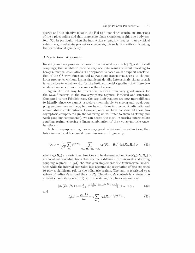
energy and the effective mass in the Holstein model are continuous functionsof the e-ph coupling and that there is no phase transition in this one-body sys-tem [36]. In particular when the interaction strength is greater than a criticalvalue the ground state properties change significantly but without breakingthe translational symmetry.

A Variational Approach

Recently we have proposed a powerful variational approach [37], valid for allcouplings, that is able to provide very accurate results without resorting toheavy numerical calculations. The approach is based on the explicit construc-tion of the GS wave-function and allows more transparent access to the po-laron properties without losing significant details. Interestingly the approachis very close to what we did for the Frohlich model signaling that these twomodels have much more in common than believed.

Again the best way to proceed is to start from very good ansatz forthe wave-functions in the two asymptotic regimes: localized and itinerant.Compared to the Frohlich case, the two limit regimes are now more difficultto identify since we cannot associate them simply to strong and weak cou-pling regimes, respectively, but we have to take into account adiabatic andnon-adiabatic contributions. However, once we have constructed these twoasymptotic components (in the following we will refer to them as strong andweak coupling components), we can access the most interesting intermediatecoupling regime choosing a linear combination of the two asymptotic wave-functions.

In both asymptotic regimes a very good variational wave-function, thattakes into account the translational invariance, is given by

|ψk >=1√N

∑Ri

eik·Ri

∑Rn,|Ri−Rn|≤d0

ηk(Ri −Rn)|φk(Ri,Rn) > (31)

where ηk(Rn) are variational functions to be determined and the |φk(Ri,Rn) >are localized wave-functions that assume a different form in weak and strongcoupling regimes. In (31) the first sum implements the translational invari-ance while the internal sum takes into account the retardation effects expectedto play a significant role in the adiabatic regime. The sum is restricted to asphere of radius d0 around the site Ri. Therefore, d0 controls how strong theadiabatic contribution in (31) is. In the strong coupling case we take

|φk(Ri,Rn) >= c†n+ie

∑q[fq(k)aqe

iq·Ri+h.c.]|0 >ph |0 >el (32)

and

fq(k) =ρq(k)ω0

= g∑Rm

|ηk(Rm)|2eiq·Rm . (33)


It is worth noting that the wave-function (31) is made by a linear com-bination of phonon coherent states (32) that, in general, describe a latticedeformation that is not centered at the electron position. Only when i = n in(32) the center of the lattice deformation and the electron position coincide.These contributions are needed to describe the electron fluctuations in thepotential well created by the lattice deformation. As already mentioned, thisfreedom in the wave-function is able to handle the adiabatic regime (γ < 1).

The wave-function (31) has been first introduced in the pioneering work byToyozawa [38] and then applied to the Holstein model in [32, 37]. If one is notinterested in the very adiabatic regime (γ � 1), it is sufficient to take threecoherent states corresponding to on site, nearest and next nearest neighbors(d0 = 2a, a being the lattice constant) to get a very good estimation ofthe GS energy. Finally we note that the form chosen for fq(k) (33) has thesame structure used in the Pekar approach for the Frohlich model [17](strongcoupling adiabatic limit). This makes the analogies between the two modelsstronger.

In the weak coupling regime we make a different choice for |φk(Ri,Rn) >.We still start from a coherent state but we only consider deformations centeredwhere the electron is sitting (d0 = 0). In this regime the polaron formation iscontrolled by the non adiabatic term. Since recoil effects are important andhave to be taken into account, we use a coherent state similar to that usedin the LLP approach for the Frohlich model. Summarizing, our choice for theweak coupling limit is:

|φk(Ri,Ri)〉 = c†i

[exp

∑q

(hq(k)aqe

iq·Ri − h.c.)]

·[1 +

∑q

d∗q(k)e−iq·Ria†

q

]|0 >ph |0 >el (34)

andhq(k) =

Mq

ω0 + Eb(q)− Eb(q = 0). (35)

Here Eb(q) is the free electron band energy:

Eb(q) = −2td∑i=1

cos(qia) (36)

where dq(k) is a variational function that has to be determined by minimizingthe expectation value of the Hamiltonian (29). We note that the term in thesquare brackets of (34) allows a considerable advantage over the independentphonon LLP approximation. In the LLP ansatz an important physical ingre-dient is missing: it does not take into account the fact that the polaron energy


Fig. 3. The polaron ground-state energy (E), the polaron kinetic energy in unitsof the bare kinetic energy (K), the average number of phonons (N) and the e-phlocal correlation function (S) are plotted as a function of g for different values of theadiabatic parameter ω0/t: ω0/t = 2.5 (solid line), ω0/t = 1 (dashed line), ω0/t = 0.5(dotted line), ω0/t = 0.25 (dashed-dotted line). The data reported are for the onedimensional case. In (a) the circles indicate the “global local variational method”data, kindly provided by A. Romero [32], and, in (b) and (d) the circles representthe DMRG data, kindly provided by E. Jeckelmann [31]. The energies are given inunits of ω0.

can approach ω0. On the contrary the wave function (34) contains this physi-cal information [39]. In particular when the polaron excitation energy becomesequal to the energy of the longitudinal optical phonon, the band dispersionflattens. For these values of k the polaron band has the bare phonon-likebehavior with very small spectral weight.

For any particular value of t there is a value of the e-ph coupling constant(gc) where the ground state energies of the two previously discussed solutionsbecome equal. Nevertheless the two solutions exhibit very different polaronfeatures. In particular when the coupling constant is smaller than gc the stablesolution (the one with lowest energy) is characterized by small lattice deforma-tions that involve many lattice sites around the electron (large polaron) whilefor g > gc it is characterized by very strong and localized lattice deformationsthat are able to trap the electron (small polaron). Crossing gc the mass of thepolaronic quasi-particle increases in a discontinuous way. A more careful in-spection shows that in this range of g values the wave functions describingthe two solutions of large and small polarons are not orthogonal and havenon-zero off diagonal matrix elements. This suggests that the lowest state ofthe system is made of a mixture of the large and small polaron solutions [40].Then the idea is to use a variational method to determine the ground state

energy of the Hamiltonian (29) by considering as trial state a linear superpo-sition of the wave functions describing the two types of previously discussedpolarons.

As in the case of the Frohlich polaron the agreement with the most ad-vanced numerical approaches is excellent (see Fig. 3).


2.3 The Su–Schrieffer–Heeger Model

In order to explain the anomalous transport properties of non-local polaronsin various 1D systems [41–44] many models have been introduced. In partic-ular the tight-binding Su–Schrieffer–Heeger (SSH) model [41] was introducedto explain the transport properties of quasi one-dimensional polymers suchas polyacetylene where the CH monomers form chains of alternating doubleand single bonds. In this case the localization is due to large shrinkage of twoparticular bonds and the corresponding large hopping integral between thesites. As a result, the hopping between the two occupied sites and the sur-rounding ones is reduced resulting in a tendency towards localization. Thisclass of models has been successfully applied to a very large number of 1Dsystems ranging from carbon nanotubes [45] to DNA [46].

Our purpose here is to examine the single polaron formation in a modelwhere non-local e-ph interactions are present (SSH model) and the phononspectrum is dispersionless. Also for this model we will use all the variationalmachinery that we discussed for the Frohlich and Holstein model showingthat, starting from a good description of the lattice deformations on the leftand right bonds of the polaron, it is possible to get a very accurate variationalGS wave-function.

If we consider only the 1D case, which is the most interesting for this classof Hamiltonians, the model takes the form

H = −t∑i

(c†i ci+1 + c†

i+1ci) + ω0

∑i

a†iai + Hint, (37)

where Hint is

Hint = gω0

∑i

(c†i ci+1 + c†

i+1ci)(a†i+1 + ai+1 − a†

i − ai), (38)

with a†i (ai) the site phonon creation (destruction) operator. The quantity g

is the dimensionless SSH coupling constant that is proportional to 4√M where

M is the ion mass. The difference with the model discussed so far is clear.The lattice deformation (xi ∼ a†

i + ai) is not coupled to the electron densitybut to the electron hopping [c†

i ci+1(xi+1−xi)] such that the electron hoppingis directly influenced by the lattice dynamics. The non-local nature of theinteraction is also clear. We study the coupling of a single electron to latticedeformations.

Variational Approach vs. Exact Diagonalization

In this section we discuss a variational approach based on the same ideasintroduced for the previous models and compare our results to exact diago-nalization of small clusters. First we introduce the variational wave function.We consider translation-invariant Bloch states obtained by superposition of


localized states centered on different lattice sites of the same type introducedin the previous section for the Holstein model. Here we extend those kind ofwave-functions to the SSH interaction model. Due to the asymmetry of theSSH coupling (shrinking of the bond on which the electron is localized andstretching of the neighboring bonds), we have to define two wave-functionsthat provide the correct description of the lattice deformations on the leftand right bonds of the polaron. Naturally the left and right directions arerelative to the site where the presence of the electron is more probable. Weassume:

|ψ(s)k 〉 =

1√N

∑i

eik·i∑n

η(s)k (n− i)|φ(s)

k (i, n)〉. (39)

where the apex s can assume the values L and R indicating the Left (L) andRight (R) polaron wave-function, respectively. In (39) we have introduced

|φ(s)k (i, n)〉 = c†

i+n exp[U

(s)k (i) + U

(s)k (i− 1) + U

(s)k (i + 1)

]|0〉ph|0〉el, (40)

with the quantity U(s)k (j) given by

U(s)k (j) =

g√N

∑q

[f (s)k,j (q)aqe

iq·Rj − h.c.]. (41)

The phonon distribution function f(s)k,j (q) is chosen as

f(s)k,j (q) =

α(s)k,j

1 + 2γβ

(s)k,j [cos(k)− cos(k + q)]

, (42)

with α(s)k,j and β

(s)k,j variational parameters. In (40), |0〉ph and |0〉el denote the

phonon and electron vacuum state, respectively, and the variational functionsφ

(s)k (i, n) are assumed to be not zero up to the fifth neighbors (|i− n| = 5). It is

worth noting that traditional variational approaches for the Holstein polaronproblem use the localized state (40) where only the on-site operator U

(s)k (i)

is applied. Thus we introduce in the expression of the trial wave-function thenearest-neighbor displacement operators U

(s)k (i + 1) and U

(s)k (i− 1), in order

to take into account the dependence of the hopping integral on the relativedistance between two adjacent ions.

The wave-functions L and R are related as follows

f(R)k,n (q) = −f (L)

k,n (q) < 0

f(R)k,n−1(q) = −f (L)

k,n−1(q) > 0

f(R)k,n+1(q) = −f (L)

k,n+1(q) > 0

φ(R)k (m) = φ

(L)k (−m). (43)


All the variational parameters are determined by minimizing the expectationvalue of the Hamiltonian (37) on the states (40). Even though the wave-functions L and R describe the different lattice deformations of the left andright side of the polaron, respectively, the mean values of the Hamiltonian onthese states are equal.

Of course the set of approximations proposed can be systematically im-proved by increasing the extension of the phonon contributions in (40) andthe number of neighbors. Furthermore, they are not orthogonal and the off-diagonal matrix elements of the Hamiltonian between these two states are notzero. This allows us to determine the ground-state energy by considering astrial state the linear superposition of the wave-functions R and L

|ψk〉 =Ak|Φ(R)

k 〉+ Bk|Φ(L)k 〉√

A2k + B2

k + 2AkBkSk. (44)

In (44) |Φ(L)k 〉 and |Φ(R)

k 〉 are the wave-functions of (39) after normalization,the coefficients Ak and Bk are the weights to be found variationally and

Sk = 〈Φ(L)k |Φ(R)

k 〉 (45)

is the overlap factor. The wave-function (44) correctly describes the propertiesof the lattice deformations on both sides of the polaron and we will find thatit is in very good agreement with the results derived by the exact diagonaliza-tions on a chain of 6 sites (see Fig. 4). Furthermore the variational approachinvolves a number of variational parameters that do not depend on the chainlength, so it allows study of the thermodynamic limit of the system.

The minimization procedure is performed in two steps. First the en-ergies of the left and right wave-functions are separately minimized, thenthese wave-functions are used in the minimization procedure of the quantityEk = 〈ψk|H|ψk〉/〈ψk|ψk〉 with respect to Ak and Bk defined in (44). Exploit-ing the equality

〈ψ(L)k |H|ψ(L)

k 〉 = 〈ψ(R)k |H|ψ(R)

k 〉 = εk, (46)

we obtain

Ek =εk − SkEkc − |Ekc − Skεk|

1− S2k

, (47)

where Ekc = 〈Φ(L)k |H|Φ(R)

k 〉 is the off-diagonal matrix element, and |Ak| =|Bk|. The matrix elements between the states ψ

(R)k and ψ

(L)k contained in (47)

are reported in [47].The results of the minimization are reported in Fig. 4 for a six-site lattice

and γ = 0.4. We also study the thermodynamic limit and find energy curvesvery close to those of the finite system. In order to test the validity of ourvariational approach, exact numerical calculations on small clusters are per-formed by means of the Lanczos algorithm. The agreement between numerical


0 0.2 0.4 0.6 0.8 1g

−3

−2.8

−2.6

−2.4

−2.2

−2

E(0

)

PT6 sites VA6 sites ED

t/ω0=1

Fig. 4. Ground state energy E(0) as a function of the SSH e-ph coupling g forγ = 0.4. Solid and dotted lines are obtained from the variational approach andthe Lanczos data for a six-site lattice, respectively; perturbative curves (dot–dashedlines) are plotted for comparison. Symbols mark the kink values of the energy.

data and variational approach is very good up to g values close to the so-calledunphysical transition. The presence of this “unphysical” transition, which issignaled by a kink in the GS energy as a function of g, deserves a brief com-ment. Indeed it has been shown [48] that the strong-coupling solution is char-acterized by an unphysical sign change of the effective next-nearest-neighborhopping which is missing when acoustical phonons are considered [43]. Forthis reason a real strong coupling regime is never reached in this model wherewe find evidence of a crossover from the weak to the intermediate couplingregime. Consequently the wave-function does not contain a strong couplingcomponent as in the models previously discussed.

As for the Frohlich model it is useful to investigate the behavior of thequasiparticle spectral weight Z(0) that signals the crossover from weak tointermediate coupling regime. We find that increasing the e-ph coupling forfixed values of γ, the spectral weight starts to drop but it never reaches areally small value before the unphysical sign change of the hopping occurs.Nevertheless we observe distinct signatures of the tendency towards local-ization. On the basis of these calculations we are able to build up a phasediagram that summarizes information on the weak to intermediate couplingand on the location of the “unphysical region” (see Fig. 5). The latter is cal-culated from the position of the kink in the ground state energy obtainedby means of the variational approach (diamonds) and exact diagonalization(triangles). The agreement between the two methods improves moving to-wards the adiabatic limit. In analogy with the phase diagram obtained forthe Holstein polaron [37], we mark a crossover region defined as the range ofparameters for which Z(0) is less than 0.9. As shown in Fig. 5, we find thatthe considered SSH model does not present any marked mixing of electronicand phononic degrees of freedom, being the strongly coupled state preventedfrom the unphysical behavior of the model. As far as the fully adiabatic limit,ω0 = 0, is concerned, we verify that the crossover line joins onto the line for


0 0.1 0.2 0.3 0.4 0.5 0.6 0.7λ

0.5

1.5

2.5

3.5

4.5

t/ωο

Unphysicalregion

Crossoverregion

Fig. 5. Phase diagram for one electron in a six-site lattice. Triangles and diamondscorrespond, respectively, to the couplings where the exact numerical ground stateenergy and the variational result have a kink. The dashed line indicates the boundaryof the crossover region, where the spectral weight Z(0) is less than 0.9.

the transition to the unphysical region at the critical value λ = 0.25, confirm-ing the discussion in [48]. We finally notice that, as discussed in [48], both thecrossover region boundary, and the instability line obtained by exact diago-nalization are only weakly dependent on the adiabatic ratio, and that λ is therelevant e-ph coupling regardless of the value of γ. This is a peculiarity of theSSH coupling with respect to the Holstein one, where the polaron crossovermoves to large values of λ as the phonon frequency increases [30, 48–50].

2.4 Intermediate and Long Range Models

The increasing interest in the effect of e-ph interaction in new materials ofpotential technological impact has not only renewed interest in studying sim-plified e-ph coupled systems such as Holstein or Frohlich models but has alsopushed researchers to propose more realistic interaction models [51, 52].

Recently a quite general e-ph lattice Hamiltonian with a “density dis-placement” type interaction has been introduced in order to understand therole of long-range (LR) coupling on polaron formation [51, 53]. The model isdescribed by the Hamiltonian

H = −t∑<i,j>

c†i cj + ω0

∑i

(a†iai +

12

)+ gω0

∑i,j

f(|Ri −Rj |)c†i ci

(aj + a†

j

).

(48)where f(|Ri − Rj |) is the interacting force between an electron on the sitei and an ion displacement on the site j and the symbol <> denotes nearestneighbors (nn) linked through the transfer integral t.

The Hamiltonian (48) reduces to the short range (SR) Holstein model iff(|Ri −Rj |) = δRi,Rj , while in general it contains longer range interaction.In particular when one attempts to mimic the non-screened coupling between


doped holes and apical oxygen in some cuprates [51], a reasonable LR expres-sion for the interaction force is given by

f(|Ri −Rj |) =(|Ri −Rj |2 + 1

)− 32 , (49)

if the distance |Ri−Rj | is measured in units of lattice constant. The expression(49) can be viewed as the natural extension of the Frohlich model to the tight-binding approximation for the electron. In addition to the SR and LR cases,we wish to analyze also intermediate coupling regimes (IR) where the electroncouples with local and nn lattice displacements. In this case the interactionfunction becomes

f(|Ri −Rj |) = δRi,Rj+

g1

g

∑δ

δRi+δ,Rj, (50)

where δ indicates the nn sites and g1 controls the corresponding couplingstrength. For all the couplings of (49,50) it is useful to define the e-ph matrixelement in the momentum space Mq as

Mq =gω0√N

∑m

f(|Rm|)eiq·Rm , (51)

and the polaronic shift Ep

Ep =∑

q

M2q

ω0. (52)

Then the coupling constant λ = Ep/zt, with z lattice coordination num-ber, represents a natural measure of the strength of the e-ph interaction inboth SR and LR cases. Clearly, for LR interactions, the matrix element Mq

peaks around q = 0. Since it has been claimed that the enhancement of theforward direction in the e-ph scattering could play a role in explaining severalanomalous properties of cuprates as the linear temperature behavior of theresistivity and the d -wave symmetry of the superconducting gap [54, 55], thestudy of lattice polaron features for LR interactions is important in order toclarify the role of the e-ph coupling in complex systems.

When the interaction force is given by (49), the model has been first inves-tigated applying a path-integral Monte-Carlo (PIMC) algorithm [51, 53] thatis able to reach the thermodynamic limit. The first investigations have beenmainly limited to the determination of the polaron effective mass pointingout that, due to the LR coupling, the polaron is much lighter than in theHolstein model with the same binding energy in the strong coupling regime.Furthermore it has been found that this effect, due to the weaker band renor-malization, becomes smaller in the antiadiabatic regime. The quasi-particleproperties have been studied by an exact Lanczos diagonalization method [56]on finite one-dimensional lattices (up to 10 sites) making a close comparisonwith the corresponding properties of the Holstein model. As a result of the

https://www.researchgate.net/publication/235499959_Lattice_polaron_formation_Effects_of_nonscreened_electron-phonon_interaction?el=1_x_8&enrichId=rgreq-5bd6b03e-52c5-4597-b1c2-df0911ce1720&enrichSource=Y292ZXJQYWdlOzIyNjgxOTg3MjtBUzoxMDExNjU5ODc1MzI4MTFAMTQwMTEzMTI2MDkxNQ==


LR interaction, the lattice deformation induced by the electron is spread overmany lattice sites in the strong coupling region giving rise to the formationof a large polaron (LP) as in the weak coupling regime. All numerical andanalytical results have been mainly obtained in the antiadiabatic and non-adiabatic regime. The behavior of the effective mass of a two-site system [57]in the adiabatic regime has been studied within the nearest-neighbor approx-imation for the e-ph interaction confirming that the LP is lighter than in theHolstein model at strong coupling. Recently we have introduced a variationalsolution [58] showing that there is a range of intermediate values of the e-phcoupling constant, in the adiabatic regime, where the GS has lost spectralweight but the polaron mass is only weakly renormalized. In the same regime,a further increase of the e-ph coupling leads to a smooth increase of the effec-tive mass associated to an average kinetic energy not strongly reduced. Thepeculiar properties of this LR model suggest investigation of the crossoverbetween short and long range coupling (intermediate coupling (IR)). This hasbeen discussed in [59] where it has been shown that for large values of thecoupling with nearest neighbor sites, most physical quantities show a strongresemblance with those obtained for the long range e-ph interaction. However,this limit is reached in a non monotonic way and, at intermediate values ofthe interaction strength, the correlation function between electron and nearestneighbor lattice displacements is characterized by an upturn as a function ofthe e-ph coupling constant.

Variational Approach

Also for this class of models (LR and IR) we can show that the variationalscheme adopted in the previous cases can be applied successfully. We consideras trial wave functions translational invariant Bloch states of the same typeof those used for the Holstein model (31). Both the weak and strong couplingcomponents can be chosen as follows:

|φ(a)k (Ri,Rn) >= c†

n+ie∑

q[f(a)q (k)aqe

iq·Ri+h.c.]|0 >ph |0 >el, (53)

where the apex a = w, s indicates the weak and strong coupling wave func-tion, respectively. Following the procedure discussed for the Holstein case, thephonon distribution functions h

(a)q (k) are chosen in order to describe polaron

features in the two asymptotic limits [37]:

h(w)q (k) =

Mq

ω0 + Eb(k + q)− Eb(k), (54)

where Eb(k) is the free electron band energy for the weak coupling case andphonon distribution function h

(s)q (k) as

h(s)q (k) =

Mq

ω0

∑Rm

|η(s)k (Rm)|2eiq·Rm (55)


Fig. 6. The ground state energy E0 in units of ω0 (a), the spectral weight Z (b), theaverage kinetic energy K (c) and the average phonon number N (d) as a functionof the coupling constant g for different values of the adiabatic ratio: ω0/t = 2 (solidline), ω0/t = 1 (dashed line), ω0/t = 0.5 (dotted line) and ω0/t = 0.25 (dash-dottedline). The diamonds in (a) indicate the PIMC data for the energy kindly providedby P. E. Kornilovitch at ω0/t = 1, and the squares on the dash-dotted line in (b)denote the ratio m/m∗ obtained within the variational approach at ω0/t = 0.25.

for the strong coupling case.Again the complete variational wave function is chosen as a superposi-

tion of weak and strong coupling components, Ak and Bk being the relativeweights.

We perform the minimization procedure with respect to the parametersη(w)k (Rm), η(s)

k (Rm), Ak and Bk, limiting the sum in (31) to third neighbors.The ground state energies obtained with this choice are slightly higher thanPIMC mean energies, the difference being less than 0.5% in the worst case ofthe intermediate regime. We note that these wave functions can, in principle,be improved extending the sum in (31) further.

In Figs. 6,7 and 8 we show some of the polaron GS properties in the one-dimensional case for LR and IR cases, respectively. We have checked thatour variational proposal recovers the asymptotic perturbative results and im-proves significantly these asymptotic estimates in the intermediate region. Inparticular, in the LR case our data for the ground-state energy in the interme-diate region are successfully compared with the results of the PIMC approach[51] shown as diamonds in Fig. 6a. The consistency of the results with a nu-merically more sophisticated approach indicates that the true wave functionis very close to a superposition of weak and strong coupling states.


Long Range Case

A specific property of the long range model is the fact that the reduction ofthe GS spectral weight is not always accompanied by an equal increase of thepolaron effective mass. This is a peculiar behavior of the LR coupling thatis completely absent in the SR Holstein model. In Fig. 6b we show that theincrease of the e-ph coupling strength induces a decrease of the spectral weightthat is smooth also in the adiabatic regime. The reduction of Z is closelyrelated to the decrease of the Drude weight obtained by exact diagonalizations[56] pointing out a gradual suppression of coherent motion. We note that thebehavior of Z is different from that of the local Holstein model. In fact, forthe latter, Z results to be very close to the ratio m/m∗, with m and m∗ bareelectron and effective polaron mass [56], respectively, while for LR couplingsZ < m/m∗ in the intermediate to strong coupling adiabatic regime. Thisrelation is confirmed by the results shown in Fig. 6b, where the dash-dottedline and the squares on a similar line indicate the spectral weight Z andthe ratio m/m∗ obtained within the variational approach, respectively, as afunction of the coupling constant g at ω0/t = 0.25 [53]. Actually there is alarge region of the parameters in the adiabatic regime where the ground stateis well described by a particle with a weakly renormalized mass but a spectralweight Z much smaller than unity. In the adiabatic case, with increasing e-phcoupling, a band collapse occurs in the SR case, while the particle undergoesa weaker band renormalization in the case of LR interactions. Therefore inthe LR case the polaron results lighter than in the SR Holstein model bothin the intermediate and strong coupling adiabatic regimes.

Insight about the electron state is obtained by calculating its kinetic energyK in units of the bare kinetic energy. Since the average kinetic energy givesthe total weight of the optical conductivity, K includes both coherent andincoherent transport processes [56]. At the same time, in the strong couplingadiabatic region before the electron self-trapping (K � 1), the average kineticenergy and the ratio m/m∗ are weakly renormalized (Figs. 6b and 6c) and,therefore, the optical conductivity is dominated by the coherent motion of thepolaron.

Another quantity associated to the polaron formation is the correlationfunction S(Rl)

S(Rl) = Sk=0(Rl) =

∑n < ψk=0|c†

ncn

(a†n+l + an+l

)|ψk=0 >

< ψk=0|ψk=0 >(56)

or equivalently the normalized correlation function χ(Rl) = S(Rl)/N , withN =

∑l S(Rl). In Fig. 7a we report the correlation function S(Rl) at ω0/t = 1

for several values of the e-ph interaction. The lattice deformation is spread overmany lattice sites giving rise to the formation of LP also in the strong couplingregime where really the correlation function assumes the largest values. In theinset of Fig. 7a the normalized electron-lattice correlation function χ shows





0 1 2 3 4 5l

-4

-3

-2

-1

0

S

0 1 2 3 4 5 λ0

0.1

0.2

0.3

0.4

0.5

χ

0 1 2 3 4 5 l

-4

-3

-2

-1

0

S

0.01 0.1 1 λ

0.1

1

ω0/t

ω0/t=1

g=2

(a) (b) (c)

Quasi-Free

Crossover

Strong

Coupling

Electron

Fig. 7. (a) The electron–lattice correlation function S(Rl) at ω0/t = 1 for differentvalues of the coupling: λ = 0.5 (circles), λ = 1.25 (squares), λ = 2.0 (diamonds),λ = 2.75 (triangles up), and λ = 3.5 (triangles down). In the inset the normalizedcorrelation function χ(Rl) at ω0/t = 1 for λ = 0.5 (circles) and λ = 2.75 (squares).(b) The electron-lattice correlation function S(Rl) at g=2 for several values of theadiabatic parameterγ = ω0: γ = 2 (circles), γ = 1 (squares), γ = 0.5 (diamonds),and γ = 0.25 (triangles up). (c) Polaron “phase diagram” for long-range (solid line)and Holstein (dashed line) e− ph interaction

consistency with the corresponding quantity calculated in a previous work[56]. While in the weak coupling regime the amplitude χ is smaller than thequantum lattice fluctuations, increasing the strength of the interaction, itbecomes stronger and the lattice deformation is able to generate an attractivepotential that can trap the charge carrier. Of course, even if the correlationsbetween electron and lattice are large, the resulting polaron is delocalized overthe lattice due to the translational invariance. Finally the variation of thelattice deformation as a function of ω0/t shown in Fig. 7b can be understoodas a retardation effect. In fact, for small ω0/t, the fewer phonons excited bythe passage of the electron take a long time to relax, therefore the latticedeformation increases far away from the current position of the electron.

On the basis of the previous discussion, in Fig. 7c, we propose a “phasediagram” based on the values assumed by the spectral weight in analogy withthe Holstein polaron. Analyzing the behavior of Z it is possible to distinguishthree different regimes: (1) quasi-free-electron regime (0.9 < Z < 1) wherethe electron has a weakly renormalized mass and the motion is coherent; (2)crossover regime (0.1 < Z < 0.9) characterized by intermediate values ofspectral weight and a mass not strongly enhanced; (3) strong coupling regime(Z < 0.1) where the spectral weight is negligible and the mass is large butnot enormous. We note that for LR interactions in the adiabatic case thereis strong mixing of electronic and phononic degrees of freedom for valuesof the coupling constant λ (solid lines) smaller than those characteristic oflocal Holstein interaction (dashed lines). Furthermore in this case, entering



the strong coupling regime, the charge carrier does not undergo any abruptlocalization, on the contrary, as indicated also by the behavior of the averagekinetic energy K, it is quite mobile.

Intermediate Range Coupling

In Fig. 8 we report some properties of the polaron ground state as a func-tion of the e-ph constant coupling λ for different g1 values that control thecoupling range. One interesting property that gives a qualitative differenceamong SR and LR models is reported in Fig. 8b. With increasing range ofcoupling, the overlapping of the two components (weak and strong) becomesmore important. Actually, as shown in Fig. 8b, there are marked differences inthe ratio B/A, that is the weight of the strong coupling solution with respectto the weak coupling one. In the SR case the strong coupling solution pro-vides almost all of the contribution. However, by increasing the range of theinteraction, the weight of the weak coupling function increases and the pola-ronic crossover becomes smoother. Another quantity that gives insight aboutthe properties of the electron state is the average kinetic energy K reportedin Fig. 8c (in units of the bare electron energy). While in the SR case K isstrongly reduced, in the LR case it is only weakly renormalized stressing thatthe self-trapping of the electron occurs for larger couplings with increasingthe range of the interaction. Finally the mean number of phonons is plottedin Fig. 8d. In the weak-coupling regime the interaction of the electron withdisplacements on different sites is able to excite more phonons. However, inthe strong coupling regime there is an inversion in the roles played by SR andIR interaction. Indeed the Holstein small polaron is strongly localized on thesite allowing a larger number of local phonons to be excited.

In addition to the quantities discussed in Fig. 8, other properties changeremarkably with increase of the ratio g1/g. An interesting property is theground state spectral weight Z. The increase of the e-ph coupling strengthinduces a decrease of the spectral weight that is more evident with increasingrange of e-ph coupling. Only in the strong coupling regime the spectral weightscalculated for different ranges assume similar small values. While for the localHolstein model Z = m/m∗, as the IR case is considered, Z becomes progres-sively smaller than m/m∗ in analogy with the behavior identified for the LRinteraction. We have found that for the ratio g1/g = 0.3 there is a regionof intermediate values of λ where the ground state is described by a particlewith a weakly renormalized mass but a spectral weight Z much smaller thanunity. Finally, we mention that, following the same criteria discussed in theprevious section it is possible to build up a phase diagram that identifies threedifferent regimes as in the case of LR coupling [59].


0 1 2 3 4 5 6 λ

0

20

40

60

80

100

B/A

0 1 2 3 4 5 6 λ

-12

-10

-8

-6

-4

-2

E0

0 1 2 3 4 5 6 λ

0

0.2

0.4

0.6

0.8

1

K

0 1 2 3 4 5 6 λ

0

4

8

12

N p

hon

(a)

(c)

(b)

(d)

Fig. 8. The ground state energy E0 in units of ω0 (a), the ratio B/A at k=0 (b),the average kinetic energy K in units of the bare kinetic energy (c) and the averagephonon number N (d) for t = ω0 as a function of the coupling constant λ for differentranges of the e− ph interaction: SR (solid line), IR with g1/g = 0.05 (dash line), IRwith g1/g = 0.1 (dot line), IR with g1/g = 0.2 (dash-dot line), IR with g1/g = 0.3(dash-double dot line), LR (double dash-dot line).

3 Excited States: Optical Conductivity and SpectralFunctions

It is well known that infrared spectroscopy is an excellent probe to investigatee-ph effects and, indeed, it was the attempt to explain the optical featuresof alkali halides by polaron absorption that motivated Landau [1] in 1933 tointroduce the notion of the self-trapped carrier. More recently, the effort inunderstanding the non-conventional properties of complex materials such astransition metal oxides and the role played by e-ph interaction, has favoreda growing interest in experimental data in such materials [60] and reliablecalculations on the optical conductivity of e-ph models.

3.1 The Frohlich Model

Although this model has attracted over the years the interest of many re-searchers [61], a complete understanding of its optical absorption has beenobtained only recently [62] by integrating many different analytical and nu-merical approaches. For a long time the understanding of this problem hasbeen mainly based on the response formalism developed by Feynman for pathintegrals [63] that, successively, has been shown to be equivalent to the mem-ory function formalism associated with the Feynman polaron model that we


Photon

Phonon

�Mq�2

Electron

Polarization

Fig. 9. The Feynman diagram used in the MFF approach eq.(58)

have discussed in Sect. (2.1)[64]. For a review of all the results obtained withinthese formalisms and, more generally, for a comprehensive account of the lit-erature on optical conductivity we refer to [65]. This approach predicts in thestrong coupling regime a sharp peak in the optical conductivity. The idea isthat, for large values of α, there is a quasi-stable state, the relaxed excitedstate (RES), characterized by lattice distortion adapted to the excited elec-tronic state. In addition to this narrow peak, a band at higher energies waspredicted. Following the interpretation of [63, 64, 66], it is due to the transi-tions to the unstable FC state. Recently, results based on the DiagrammaticQuantum Monte Carlo (DQMC) methods [62, 67] have shown that there is noindication of any sharp resonance in the infrared spectra. From this analysisit is clear that going beyond the approximations used so far is crucial in orderto clarify the different aspects of the problem [62].

From Weak to Intermediate Coupling Optical Conductivity

A description of the infrared absorption, able to reproduce the main structureof DQMC data up to α � 8, can be obtained by using the memory functionformalism (MFF)[68]. Within this approach the real part of the conductivity,in the limit of a vanishing electron density n, and treating the interactionbetween the charge carriers and the phonons at the lowest order, can bewritten as [63, 64]

Re [σxx(ω)] = −ne2

m

Im [Σxx(ω)](ω − Re [Σxx(ω)])2 + (Im [Σxx(ω)])2

(57)

where

Im [Σxx(ω)] =1

mω

∑q

|Mq|2 q2xIm [χ(q, ω − ω0)] (58)

and


χ(q, t) = −iθ(t)⟨eiq·r(t)e−iq·r(0)

⟩. (59)

In term of Feynman diagrams (58) corresponds to the phononic renormal-ization of the electron polarization bubble (Fig. 9). Of course, the key role inthe MFF is played by the calculation of the Fourier transform of the electrondensity-density correlation function: χ(q, t). At the lowest level it can be cal-culated assuming that the electron does not interact with phonons and givesχ(q, t) = −iθ(t) exp

[−iq2t/(2m)

]. This approximation returns the perturba-

tive result (α� 1)

Im [Σxx(ω)] = −23αω

3/20

ω

√ω − ω0θ(ω − ω0).

This quantity has been traditionally evaluated (see [63]) by using the FPMin which the electron is coupled via a harmonic force to a fictitious particlesimulating the phonon degrees of freedom. The result is

χ(q, t) = −iθ(t)e−i q2t2Me e− q2R

2Me(1−e−ivt) (60)

where Me = m v2

w2 is the total mass of FPM and R = v2−w2

vw2 . v and w arerelated to the mass and the elastic constant of the model and are determinedvariationally (see Sect. (2.1)). Consequently Im [Σxx(ω)] becomes:

Im [Σxx(ω)] = −2αv3ω3/20

3ωw3

∞∑n=0

θ(ωn)n!

exp

[−ωn

(v2 − w2

)vw2

] (v2 − w2

)nvnw2n ωn+1/2

n

(61)where ωn = ω − ω0 − nv. As already mentioned, the majority of the work onoptical conductivity, given by (57), is based on (61). However, it contains twoimportant limitations. The first one is that the exact sum rule

∞∫−∞

dω

πω2Im [χ(q, ω)] = −

(q2

2m

)2

− 23q2

m

⟨p2

2m

⟩(62)

is not satisfied and the other one is that this approximation does not containdissipative effects. Both limitations can be removed introducing a finite life-time in (60) in such a way that the sum rule (62) is fulfilled. Lifetime effectsare expected to play a strong role since the FPM is only an effective modelthat only partially takes into account the phonon bath and a residual cou-pling with the original bath should still have important effects. If we replacethe term e−ivt in (60) with (1 + it/τ)−vτ we allow the FPM to scatter withthe phonon bath attributing finite lifetimes to the states of the FPM. Thequantity τ is determined making use of the sum rule (62) where

⟨p2

2m

⟩is es-

timated by using Feynman approach for the polaron ground state. We stress


Fig. 10. The OC for different values of α calculated within the EMFF (solid line).Our EMFF data are compared with weak coupling perturbation theory (dotted line),MFF (dashed line) and DQMC data (open circles).

here the difference between Feynman approach and FPM. In the former thescattering among the FPM and the residual e-ph interaction is included. Itis worthwhile noting that for τ −→ ∞ we recover the expression (60). Wewill call this approximation extended memory function formalism (EMFF).As expected, τ turns out to be of the order of ω−1

0 . In Fig. 10 we comparethe results with DQMC and with the theory based on (61). In the weak e-phcoupling regime, the memory function formalism, with or without damping τ ,is in good agreement with DQMC data, indicating that the phonon assistedintra-band transitions are dominant in this regime (Fig. 10a). In any case theresults shown (Figs. 10b,10c) exhibit a significant improvement with respectto weak coupling perturbation approach [69]. The latter of these, which isrecovered within the memory function formalism, provides a good descrip-tion of the infrared spectra only for very small values of α. As the plots inFig. 10d show, the introduction of the damping becomes crucial already atα = 4.5. Here the agreement with DQMC data is still complete while theresults obtained neglecting the damping provide a sharper peak in the opticalconductivity that is not present in the DQMC data. On the other hand, atα = 6 the optical conductivity calculated within DQMC starts to present asmall shoulder that is not present in our EMFF. In the next section we willtry to understand this new structure starting from the opposite limit of strongadiabatic coupling.

Strong Coupling Optical Conductivity: Franck-Condon Regime

For α >> 1, as discussed in Sect. 2.1, the GS of the Frohlich model is welldescribed by the adiabatic approximation and, therefore, we expect that inthis regime, the OC is dominated by the Franck-Condon (FC) principle [70]that rests on the adiabatic decoupling of electron and lattice degrees of free-dom. We present, here, a derivation of OC in the FC limit that includes

https://www.researchgate.net/publication/253758048_Optical_Process_in_Solids?el=1_x_8&enrichId=rgreq-5bd6b03e-52c5-4597-b1c2-df0911ce1720&enrichSource=Y292ZXJQYWdlOzIyNjgxOTg3MjtBUzoxMDExNjU5ODc1MzI4MTFAMTQwMTEzMTI2MDkxNQ==


phonon replica. As we will see this approach is able to reproduce correctly theapproximation-free results of DQMC for large enough α.

Following the Landau-Pekar approach (6)-(15), we first apply the canonicaltransformation U = exp

[−∑

q((ρq/ω0) aq − h.c.)]

to the Frohlich Hamilto-nian and obtain

H =p2

2m+∑

q

ω0a†qaq +

∑q

[(Mqe

iq·r − ρq)aq + h.c.]

(63)

−∑

q

[ρ∗q

ω0(Mqe

iq·r − ρq) + h.c

]−∑

q

|ρq|2

ω0

where ρq = Mq〈ϕ|eiq·r|ϕ〉 (8) is related to the GS electron wave-function|ϕ〉. It has to be emphasized that the use of the canonical transformation,U , breaks the translational invariance, but this is not a severe limitation inthe strong coupling limit. The Hamiltonian (63) can be viewed as a FrohlichHamiltonian with a modified e-ph coupling function in an external potentialgiven by the last two terms. In order to proceed further in the OC calculationwe have to make a further approximation replacing in (63) the true potentialwith an harmonic one (see (11)). This allows us to identify in (63) a part thatcan be solved exactly (the sum of a harmonic oscillator and free phonons)and the part that we wish to treat perturbatively. Summarizing, we obtainH → H = H0 +

∑q ω0a

†qaq +W where:

H0 =p2

2m+

mω2

2r2 − 3

4ω; and W =

∑q

[(Mqe

iq·r − ρq)aq + h.c.]. (64)

ω = (4α2ω0)/(9π) is the Landau-Pekar variational estimation (13). It is worthnoting that the estimation of the energy difference between the GS and thefirst adiabatic excited state can be improved exploiting the derivation of theFeynman approach presented in Sect. 2.1. In that formalism we can choose atrial wave-function like that of (4) where the GS of FPM is replaced with thefirst electronic excited state. Actually we keep the phonon potential well fixedat the value found for the GS, but we put the electron in the first excitedstate. This gives the following value for ω = (4α2ω0)/(9π)− 3.8ω0.

Since the real part of the OC in the limit of vanishing electron density canbe written in terms of the position operator

Re [σxx(ω)] = ne2ωRe

∞∫0

dtei(ω+iδ)t 〈x(t)x(0)〉

we have to evaluate 〈x(t)x(0)〉 by using the Hamiltonian of (64). Within thisset of approximations it is possible to eliminate exactly the phonon degreesof freedom showing that


〈x(t)x(0)〉 =1

2mωe−iωt 〈f1,0,0f |Teχ| f1,0,0〉

where |f1,0,0〉 is the first excited state of H0, T is the time ordering operatorand

χ(t) = −t∫

0

dτ

τ∫0

dτ ′e−iω0(τ−τ ′)∑

q

wq(τ)w∗q (τ

′). (65)

In (65) wq(s) = exp[iH0s

](Mqe

iq·r − ρq) exp[−iH0s

]. At this stage of the

calculation, if we completely neglect χ, we recover the extreme FC regime inthe Landau-Pekar approximation:

Re [σxx(ω)] =ne2π

2mδ(ω − ω).

In order to include higher order contributions we make two further ap-proximations. First we neglect the time correlations:

〈f1,0,0f |Teχ| f1,0,0〉 → exp 〈f1,0,0 |χ| f1,0,0〉

and then retain in⟨f1,0,0

∣∣wq(s)w∗q (s

′)∣∣ f1,0,0

⟩only those terms that do not

depend on (s− s′). While the first approximation is motivated by a real com-putational difficulty (even if we do not expect that time correlations are im-portant at α >> 1) , the second one is based on the fact that ω0 � ω. Theinclusion of the terms proportional to (s− s′) can be done exactly and shouldtake into account the first non-adiabatic contributions. We get


2mω

ω

∞∑n=0

exp[−ωsω0

](ωsω0

)n 1n!

δ (ω − ω + ωs − nω0) ,

where ωs = α√

ωω30/(4

√π). This expression is very close to that expected for

the exactly solvable independent oscillators model [71]. The OC contains a setof delta function peaks starting from (ω−ωs) and separated by ω0. However,for α >> 1, the maximum spectral weight is attributed to the peak closest toω, the FC frequency. The effect of the residual e-ph scattering does not changethe peak maximum, but introduces phonon sidebands that concur to define aneffective peak width. This becomes clearer for large enough coupling strengths(or, equivalently, for ω0 → 0) when the envelope of the Poisson distributioncan be described by the Gaussian


2mω

ω

1√2πω0ωs

exp{− (ω − ω)2

2ω0ωs

}. (66)

The frequency (ω−ωs) deserves a comment. Indeed, it can be interpretedas the RES introduced by Devreese [61], but, at the strong coupling regime


Fig. 11. The OC for different values of α calculated within the SC approach (solidline). Our SC data are compared with MFF (dashed line) and DQMC data (opencircles).

where the present derivation is valid it has only a marginal spectral weight.Within this approximate scheme we cannot judge if in the intermediate cou-pling regime RES could play some role.

In Fig. 11 the very good agreement between the adiabatic SC approach andthe DQMC data clearly shows that the broad peak observed in the DQMCdata at α >> 1 is due to FC processes. We have also reported the MFFresult for comparison. In this regime, it reduces to a delta function locatedat the FC energy and to a very small structure at higher energy. Both thesestructures follow the α2 dependence characteristic of the FC transition. Thisbehavior suggests that the MFF, even if it completely misses the correct OCpeak shape, is able to reproduce the FC energy.

We end this section mentioning that the results obtained both in the weakto intermediate coupling and in the strong coupling regime are in very goodagreement with DQMC data [62]. We refer to the chapter by Mishchenko andNagaosa [72] for a specific account of those data. Here, we wish to stress thatfrom the analysis outlined here and from DQMC data a clear scenario comesout. We find that different regimes, characterized by different excitations, canbe recognized. i) For large values of α, α ≥ 11, the main contribution to thereal part of the optical conductivity comes from the transition to the firstexcited state in the potential well characteristic of the polaron ground state.In this regime the spectral weight of the RES turns out to be negligible. Fur-thermore, the maximum of the optical conductivity follows the characteristicdependence predicted for the energy gap between the ground and FC states,i.e. it is proportional to 4α2/9π; ii) in the opposite regime (α ≤ 1), as shown bythe perturbation theory, the maximum of the optical conductivity is relatedto the phonon assisted intra-band transitions. The spectral weight of theseoptical transitions decreases with increasing strength of the e-ph interaction;iii) for 1 ≤ α ≤ 6, in addition to the phonon assisted intra-band transitions,which still survive, the main contribution to the real part of the conductivity


Fig. 12. (a) and (b). The OC for different values of α calculated within the EMFF(solid line) and SC approach (dotted line). Our data are compared with MFF(dashed line) and DQMC data (open circles). (c) The polaron effective mass asfunction of α [13].

comes from the electron transitions between the damped levels of the FPM.Here the interaction with free lattice oscillations is treated at the lowest orderand the dynamic lattice effects are dominant. In any case we can say that,for these values of α, the FPM captures also the physics of the excited statesof the Frohlich model; iv) at α = 7 a new excitation is present in the opticalabsorption. The DQMC data [67] exhibit a shoulder at ω � 4ω0. At α = 8.5two structures appear in the infrared spectra with almost the same spectralweight. This new excitation is due to the FC transitions, i.e. the lattice con-figuration does not change during the radiation absorption process. At thisvalue of α static and dynamic lattice effects coexist (see Fig. 12). We endthis section showing that the previous scenario is confirmed by the effectivepolaron mass behavior (see Fig. 12). Also for this quantity we can identifythree regimes that correspond to the different OC regions: i) α < 6 where thepolaron mass enhancement is not very strong and the lattice is still able topartially follow the electrons; ii) α > 9 where the lattice is completely staticand the mass is huge; iii) 6 < α < 9 where the mass makes its rapid crossoverbetween small and very large values and static and dynamic features coexistsin the OC.

3.2 The Holstein Model

Spectral Function in the Coherent State Basis

Knowledge of the spectral function is crucial to get information on the ex-cited states of any system and is directly related to photoemission experi-ments. In particular, the great importance played by this class of experimentsin cuprates has renewed the interest in non perturbative calculation for thespectral function of the Holstein model. The open question is whether or notsome spectroscopic features can be attributed to e-ph interaction [4, 73].


Recently a large number of numerically exact methods have been intro-duced. These approaches are based on different algorithms for exact diagonal-ization [28], but all need some kind of truncation in the phonon space. Theintroduction of an optimized phonon approach based on the analysis of thedensity matrix [31, 74] has produced an important improvement in this field.The idea is to exploit the knowledge of the largest eigenvalues and eigenvectorsof the site density matrix to select the phonon linear combinations that, at thebest, can describe the system: the so-called optimized phonon basis (OPB).Unfortunately, the density matrix of the target states is not available a priori :it must be calculated in a self-consistent way together with the OPB. To thisaim different strategies have been discussed. Recently, we have introduced avariational technique, based on an expansion of coherent states (CS) that verymuch simplifies the selection of an optimized phonon basis and that does notrequire any truncation in the number of phonons [75, 76]. This method is ableto provide accurate results for any e-ph coupling regime and for any value ofthe adiabatic ratio. In the Holstein model, the proposed expansion providesstates surprisingly close to the eigenvectors of the site density matrix corre-sponding to the highest probabilities. Although the method requires a smallerphonon basis with respect to previous proposals, it has been applied so far torelatively small clusters. The idea is to replace the “natural” phonon basis ateach site i |µi〉 with a coherent state |h, i〉:

|µi〉 → |h, i〉 = egh(bi−b†i ) |0〉(ph)

i = e− g2h2

2

∞∑n=0

(−gh)n√n!

|n〉i . (67)

This substitution does not introduce any truncation in the Hilbert space since,varying h in the complex plane, the local basis (67) is over-complete. In par-ticular, for h = 0, the CS |h = 0, i〉 is the phonon vacuum at site i, i.e. thephonon ground state at site i when g = 0 (absence of e-ph interaction). Onthe other hand, for h = 1, the CS |h = 1, i〉, multiplied by the product of thephonon vacuum on the remainder of the sites,

∏j �=i |0〉

(ph)j , gives the ground

state of the Holstein Hamiltonian when t = 0, i being the site which theelectron occupies.

However, in order to perform a numerical diagonalization of the HolsteinHamiltonian, we need to work with a finite number of coherent states. To thisaim the second step is to choose a finite number M of CS, characterized bythe corresponding values hα (α = 0, ...,M − 1), that we choose to be realand assume to be independent on the site index i. Then we consider only thephonon states

∏Ni=1 |hαi

, i〉, with∑N

i=1 αi ≤ (M − 1). Taking into accountthat the coherent state |h, i〉 is a linear superposition of states with fixednumber of phonons (see (67)) distributed according to the Poisson functionwith a maximum at n � (hg)2 and variance σ2 = (hg)2, it easy to recognizethat the previous procedure does not introduce any truncation in energy andin the phonon number. In particular the mean value and the variance increaseby increasing the values of h and g. Then, when the e-ph interaction is strong


Fig. 13. The spectral weight function A(k, ω)/ (2π) at t/ω0 = 2.5 and k = 0 forthree different values of the e-ph coupling constant. In Fig. 3c, for comparison, theLang-Firsov [26] spectral function is reported (dotted line). The arrows indicatethe ground state energy. The energies are in units of ω0. The value of the cutoff isM = 16 and the number of sites is N=8.

and h is of the order of one, the CS |h, i〉 represents a state with a largeenergy and phonon number dispersion and then it is the ideal candidate todescribe small–polaron physics. In this case the presence, in the chosen basis,of coherent states with a small value of h allows us to take into account alsothe quantum fluctuations and the retardation effects of the e-ph interaction.

The ground state is obtained by using the modified Lanczos method [77].We obtain a systematic improvement of the approximation adding more andmore CS and this allows us to estimate the error introduced by a specifictruncation. The variational calculation always provides values of h such that0 ≤ h ≤ 1. In particular, when the value of the cutoff M is about or greaterthan 10 the variationally chosen values of h turn out to be equally distributedwithin the interval [0, 1]. The main advantage of this approach is that theconvergence of the ground state energy is very rapid so that we obtain thebest subspace in which to find the target state with a little numerical effort,independently of the value of the e-ph coupling constant. This behavior can beunderstood by studying the site density matrix. In fact, we have shown in [75]that for a two-site one-electron system the eigenvectors corresponding to thelargest eigenvalues of the exact site density matrix are in excellent agreementwith those obtained in our approach, already with two CS per site.

In order to appreciate the computational improvement that can be ob-tained by using the coherent state basis we show in Fig. 13 the spectral weightfor different values of the coupling constant in the moderate adiabatic regime.


Optical Conductivity

Following the analysis presented for the Frohlich model we can calculate,also for the Holstein model, the OC in two limiting cases by using the MFFand the adiabatic FC approximation, respectively. Once again it is worthnoting that that Frohlich and Holstein models have many more similaritiesthan expected. As discussed for the Frohlich model, for the Holstein modelwe can also individuate a weak coupling regime dominated by intra-bandexcitations (Sect. 3.1) where dynamic phonon processes are relevant and anadiabatic strong coupling limit where only Franck-Condon processes betweenlocalized electron states contribute to the OC [78]. In the former case the MFFprovides an excellent description of the relevant processes. Following closelythe procedure outlined in Sect. 3.1 it is possible to obtain the OC that, in the1D case, takes the closed form:

Re [σ(ω)] = −2te2

N

Im [Σ(ω)](ω − Re [Σ(ω)])2 + (Im [Σ(ω)])2

,

where

Im [Σ(ω)] = −g2ω20

ω

√1− (ω − ω0 − 2t)2

4t2θ(ω − ω0)θ(ω0 − ω + 4t).

The real and imaginary parts of Σ(ω) are related by the usual Kramers-Kroning relations. In the adiabatic strong coupling limit we can proceed as inSect. 2.2. Within the same set of approximations we get the following expres-sion for the OC:

Re [σxx(ω)] =e2π

Nωβ2

∞∑n=0

exp[−ωsω0

](ωsω0

)n 1n!

δ (ω − ω + ωs − nω0)

where ωs = 3g2ω0α4/2, and ω = E1 − E0. The quantity E1 − E0 is the

energy difference between ground and first adiabatic excited states that can becalculated, for instance, with the variational approaches discussed in Sect. 2.2and β =

⟨f

(0)el

∣∣∣Px ∣∣∣f (1)el

⟩is the matrix element of the x component of the

electron position in the tight-binding approximation between the ground state(∣∣∣f (0)el

⟩) and the first adiabatic excited state (

∣∣∣f (1)el

⟩). Finally α is related

to β via the normalization condition |α|2 + d |β|2 = 1, d being the systemdimensionality.

While those two limiting cases are well established in the literature thequestion of the Holstein OC in the intermediate coupling is still open. Howdoes the crossover proceed between these limits? One possibility is that inthe Holstein case the crossover regime is also characterized by the presence ofboth types of processes making the Frohlich and Holstein models even more


similar. Another possibility is that the crossover regime is characterized bynew processes that are not relevant in the asymptotic limits. One proposalin this sense is given in [79] where adiabatic photoemission processes areconsidered responsible for the OC in the regime characterized by gω0 � 4dt.We end this section mentioning that such process has been already proposedby Emin [80] for the OC of Frohlich model, even if there is no evidence forthem in the error free DQMC data [62].

4 Conclusion

In this chapter we have discussed the polaron formation and some of its prop-erties in a number of e-ph models by using a unifying variational point ofview. We have shown how variational semi-analytical approaches can give avery accurate description of these systems without resorting to heavy numeri-cal calculations. These are crucial in order to have a reference point in the nonperturbative regimes, but semi-analytical approaches have the advantage ofgiving direct access to the ground state wave-function making the understand-ing of the physical properties more transparent. A paradigmatic example ofthis statement is the case of Frohlich OC where the joint effort of DQMC andsemi-analytical results has been crucial in disentangling the complex physicsof that model. We firmly believe that the merger of these different approacheswill produce new and important improvements in the polaron field.

Acknowledgement. Let us finish by thanking G. Iadonisi, V. Marigliano Ramaglia,M. Capone, E. Piegari, S.A. Mishchenko and J. Devreese, for discussions and col-laborations.

References

1. L.D. Landau: Phys. Z. Sowjetunion 3, 664 (1933) [English translation: CollectedPapers (Gordon and Breach New York, 1965), pp.67-68];

2. R.P. Feynman: Phys. Rev. 97,660 (1955).3. D.M. Edwards: Adv. Phys. 51, 1259 (2002); E. Dagotto, Nanoscale phase sep-

aration and colossal magnetoresistance: the physics of manganites and relatedcompounds (Springer, Heidelberg New York 2003).

4. Lattice effects in High Temperature Superconductors ed by Y. Bar.Yam, J. Mus-tre de Leon, and A. R. Bishop (World Scientific, Singapore, 1992); A. Damas-celli, Z. Hussain, and Zhi-Xun Shen, Rev. Mod. Phys. 75, 473 (2003); P.A. Lee,N. Nagaosa, and X.-G. Wen: Rev. Mod. Phys. 78, 17 (2006).

5. J. Zaanen and P.B. Littlewood: Phys. Rev. B 50, 7222 (1994); G. Wu and J.J.Neumeier: Phys. Rev. B 67, 125116 (2003); Hotta Takashi and E. Dagotto:Phys. Rev. Lett. 92, 227201 (2004). .

6. J.W. Bray, L.V. Interrante, L.S. Jacobs, and J.C. Bonner in Extended lin-ear Chain Compounds, ed by J.S. Miller (Plenum, New York, 1985), p. 353;


S. Kagoshima, H. Nagasawa, and T. Sambongi One-Dimensional Conductors(Springer-Verlag, New York, 1988).

7. H. Frohlich, H. Pelzer, and S. Zienau: Philos. Mag. 41, 221 (1950).8. G. Hohler and A.M. Mullensiefen: Z. Physik 157, 159 (1959); D.M. Larsen:

Phys. Rev. 144, 697 (1966); G.D. Mahan: in Polarons in Ionic Crystalsand Polar Semiconductors (North-Holland, Amsterdam, 1972), p. 553; M.A.Smondyrev: Teor. Mat. Fiz. 68, 29 (1986).

9. N.N. Bogoliubov and S.V. Tiablikov: Zh. Eksp. i Theor. Fiz., 19, 256 (1949);S.V. Tiablikov: Zh. Eksp. i Theor. Fiz., 21, 377 (1951); S.V. Tiablikov Abhandl.Sowj. Phys., 4, 54 (1954); G.R. Allcock: Advances in Physics 5, 412 (1956); G.Hohler in Field Theory and the Many Body Problem, ed. E.R. Caianiello (Acca-demic Press), pp.285; E.P. Solodovnikova, A.N. Tavkhelidze, O.A. Khrustalev:Teor. Mat. Fiz. 11, 217 (1972); V.D. Lakhno and G.N. Chuev: Physics-Uspekhi38, 273 (1995).

10. D. Dunn: Can. J. Phys., 53, 321 (1975).11. T.D. Lee, F. Low, and D. Pines: Phys. Rev. 90, 297 (1953); M. Gurari: Phil.

Mag., 44, 329 (1953); E.P. Gross: Phys. Rev., 100, 1571 (1955); G. Hohler:Z. Physik, 140, 192 (1955); G. Hohler: Z. Physik, 146, 372 (1956); Y. Osaka:Prog. Theor. Phys., 22, 437 (1959); T.D. Schultz: Phys. Rev., 116, 526 (1959);D.M. Larsen: Phys. Rev., 172, 967 (1968); J. Roseler: Phys. Stat. Sol., 25, 311(1968).

12. N.V. Prokof’ev and B. V. Svistunov: Phys. Rev. Lett. 81, 2514 (1998).13. A.S. Mishchenko, N.V. Prokof’ev, A. Sakamoto, and B.V. Svistunov: Phys.

Rev. B 62,6317 (2000).14. John T. Titantah, Carlo Pierleoni, and Sergio Ciuchi: Phys. Rev. Lett., 87,

206406 (2001).15. An interesting discussion on the accuracy of Feynman’s polaron model can be

found in J.T. Devreese and R. Evrard: Phys. Lett. 11, 278 (1964).16. G. De Filippis, V. Cataudella, V.M. Ramaglia, C.A. Perroni and D. Bercioux:

Eur. Phys. J B 36, 65 (2003).17. L.D. Landau and S.I. Pekar: J. Exptl. Theor. Phys. 18, 419 (1948); S.I. Pekar:

Research in Electron Theory of Crystals, Moscow, Gostekhizdat (1951) [Englishtranslation: Research in Electron Theory of Crystals, US AEC Report AEC-tr-5575 (1963)].

18. S.J. Miyake: J. Phys. Soc. Jap. 38, 181 (1975); 41, 747 (1976).19. T.D. Lee, F. Low, and D. Pines: Phys. Rev. 90, 297 (1953).20. D.N. Larsen: Phys. Rev. 172,967 (1968).21. G. Hohler and A.M. Mullensiefen: Z. Physik 157,159 (1959).22. J. Roseler: Phys. Stat. Sol. 25, 311 (1968).23. T. Holstein: Ann. Phys. (Leipzig) 8, 325 (1959).24. A. B. Migdal: Sov. Phys. JETP 7, 996 (1958).25. A. A. Gogolin: Phys. Status Solidi 109, 95 (1982); F. Marsiglio: Physica C 244,

21 (1995); W. Stephan: Phys. Rev. B 54, 8981 (1996).26. I.J. Lang, and Yu. Firsov: Sov. Phys. JEPT 16, 1301 (1963).27. H. de Raedt and Ad Lagendijk: Phys. Rev. B 27, 6097 (1983) and Phys. Rev.

B 30, 1671 (1984); P. E. Kornilovitch: Phys. Rev. Lett. 81, 5382 (1998); M.Hohenadler, H.G. Evertz, and W. von Linden: Phys Rev. 69, 24301 (2004).

28. For a review see: E. Jeckelmann and H. Fehske:Exact numerical methods forelectron phonon problems. In: Polarons in Bulk Materials and Systems with


Reduced Dimensionality, ed. by G. Iadonisi, J. Ranninger and G. De Filippis(IOS Press Amsterdam, Oxford, Tokio, Washington DC, 2006), p.247.

29. A. Kongeter and M. Wagner: J. Chem. Phys. 92, 4003 (1990); J. Ranninger andU. Thibblin: Phys. Rev. B 45, 7730 (1992); A. S. Alexandrov, V. V. Kabanovand D. K. Ray: Phys. Rev. B 49, 9915 (1994); E. de Mello and J. Ranninger:Phys. Rev. B 55, 14872 (1997); M. Capone, W. Stephan, and M. Grilli: Phys.Rev. B 56, 4484 (1997); G. Wellein and H. Fehske: Phys. Rev. B 56, 4513(1997); H. Fehske, J. Loos, and G. Wellein: Z. Phys. B 104, 619 (1997).

30. S. Ciuchi, F. de Pasquale, S. Fratini, and D. Feinberg: Phys. Rev. B 56, 4494(1997); S. Ciuchi, F. de Pasquale, and D. Feinberg: Physica C 235-240, 2389(1994).

31. S. R. White: Phys. Rev. B 48, 10345 (1993); E. Jeckelmann and S. R. White:Phys. Rev. B 57, 6376 (1998).

32. A. H. Romero, D. W. Brown, and K. Lindenberg: Phys. Rev. B 59, 13728(1999); 60, 14080 (1999); 62, 1496 2000; J. Comp. Phys. 109, 6540 (1998).

33. G. Iadonisi, V. Cataudella, G. De Filippis, and D. Ninno: Europhys. Lett. 41,309 (1998); G. Iadonisi, V. Cataudella and D. Ninno: Phys. Sta. Sol. (b) 203,411 (1997); Y. Lepine and Y. Frongillo: Phys. Rev. B 46, 14510 (1992).

34. J. Bonca, S.A. Trugman and I. Batistic: Phys. Rev. B 60, 1633 (1999); L.C.Ku, S.A. Trugman, and J. Bonca; Phys. Rev. B 65, 174306 (2002).

35. O.S. Barisic: Phys. Rev B 65, 144301 (2002).36. H. Lowen: Phys. Rev. B 37, 8661 (1988); B. Gerlach and H. Lowen: Rev. Mod.

Phys. 63, 63 (1991).37. V. Cataudella, G. De Filippis and G. Iadonisi: Phys. Rev. B 60, 15163 (1999);

62, 1496 (2000).38. Y. Toyozawa: Prog. Theor. Phys. 26, 29 (1961).39. D.N. Larsen: Phys. Rev. 144, 697 (1966).40. D.N. Eagles: Phys. Rev. B, 145,645 (1966).41. W. P. Su, J. R. Schrieffer, and A. J. Heeger: Phys. Rev. Lett. 42, 1698 (1979);

Phys. Rev. B 22, 2099 (1980).42. Solitons and Polarons in Conducting Polymers, ed by Y. Lu (World Scientific,

Singapore 1988).43. A. La Magna and R. Pucci: Phys. Rev. B, 55, 6296 (1997).44. M. Zoli: Phys. Rev. B 66, 012303 (2002); 67, 195102 (2003).45. M. Verissimo-Alves, R. B. Capaz, B. Koiller, E. Artacho, and H. Chacham:

Phys. Rev. Lett. 86, 3372 (2001); E. Piegari, V. Cataudella, V. Marigliano,and G. Iadonisi: Phys. Rev. Lett. 89, 49701 (2002); Yu N. Gartstein, A. A.Zakhidov, and R. H. Baughman: Phys. Rev. Lett. 89, 045503 (2002).

46. S. S. Alexandre, E. Artacho, J. M. Soler, and H. Chacham: Phys. Rev. Lett.91, 108105 (2003).

47. CA Perroni, E. Piegari, M. Capone and V. Cataudella: Phys. Rev. B 69, 174301(2004).

48. M. Capone, W. Stephan, and M. Grilli: Phys. Rev. B 56, 4484 (1997).49. M. Capone, S. Ciuchi, and C. Grimaldi: Europhys. Lett. 42, 523 (1998).50. M. Capone and S. Ciuchi: Phys. Rev. Lett. 91, 186405 (2003).51. A. S. Alexandrov and P. E. Kornilovitch: Phys. Rev. Lett. 82, 807 (1999).52. A. W. Sandvik, D. J. Scalapino, and N. E. Bickers: Phys. Rev. 69, 94523 (2004).53. A. S. Alexandrov: Phys. Rev. B 61, 12315 (2000); A. S. Alexandrov and C.

Sricheewin: Europhys. Lett. 51, 188 (2000).


54. E. Cappelluti and L. Pietronero: Europhys. Lett. 36, 619 (1996).55. M. L. Kulic: Phys. Rep. 338, 1 (2000).56. H. Fehske, J. Loos, and G. Wellein: Phys. Rev. B 61, 8016 (2000).57. A. S. Alexandrov and B. Ya. Yavidov: Phys. Rev. B 69, 73101 (2004).58. C.A. Perroni, V. Cataudella, G. De Filippis: J. Phys.: Condens. Matter 16,

1593 (2004).59. C.A. Perroni, V. Cataudella, G. De Filippis: Phys. Rev. B 71, 54301 (2005).60. For a recent review see P. Calvani: Effects of strong charge-lattice coupling on

the optical conductivity of transition-metal oxides. In Polarons in Bulk Materi-als and Systems with Reduced Dimensionality, ed. by G. Iadonisi, J. Ranningerand G. De Filippis (IOS Press Amsterdam, Oxford, Tokio, Washington DC,2006), p.53.

61. For a review see J.T. Devreese: Polarons. In Encyclopedia of Applied physics,edited by G.L. Trigg (VCH, New Jork, 1996), Vol. 14, p. 383.

62. G. De Filippis, V. Cataudella, A. Mishchenko, C.A. Perroni, and J. Devreese:Phys.Rev. Lett. 96, 136405 (2006).

63. J.T. Devreese, J. De Sitter, and M. Govaerts: Phys. Rev. B 5, 2367 (1972);see also J.T. Devreese: Internal structure of the free Frohlich Polaron, opticalabsorption and cyclotronic resonance. In Polarons in ionic crystals and polarsemiconductors (North-Holland, Amsterdam 1972) p. 83

64. F.M. Peeters and J.T. Devreese: Phys. Rev. B 28, 6051 (1983).65. J.T. Devreese, this volume66. E. Kartheuser, R. Evrard, and J. Devreese: Phys. Rev. Lett. 22, 94 (1969).67. A.S. Mishchenko, N. Nagaosa, N.V. Prokofev, A. Sakamoto, and B.V. Svis-

tunov: Phys. Rev. Lett. 91, 236401 (2003).68. H. Mori: Prog. Theor. Phys. 33, 423 (1965); 34, 399 (1965); W. Gotze, and P.

Wolfle: Phys. Rev. B 6, 1226 (1972).69. V.L. Gurevich, I.E. Lang, and Yu A. Firsov: Fiz. Tverd. Tela: 4, 1252 (1962)

[Sov.Phys. Solid State 4, 918 (1962)]; G.D. Mahan: Many-Particle Physics,(Plenum, New Jork, 1981), Chap. 8.

70. Y. Toyozawa, Optical Processes in Solids, (Cambridge: University Press, 2003).71. G.D. Mahan: Many-Particle Physics, (Plenum, New Jork, 1981), Chap. 4, pag.

282.72. A.S. Mishchenko and N. Nagaosa, this volume.73. K.M. Shen, F. Ronning, D.H. Lu, W.S. Lee, N.J.C. Ingle, W. Meevasana,

F. Baumberger, A. Damascelli, N.P. Armitage, L.L. Milelr, Y. Kohaska, M.Azuma, M. Takano, H. Takagi, and Z.-X. Shen: Phys. Rev. Lett. 93, 267002(2004).

74. G. Wellein and H. Fehske: Phys. Rev. B 58,6280 (1998); A. Weisse, H. Fehske,G. Wellein, and A. R. Bishop: Phys. Rev. B 62 R747 (2000).

75. V. Cataudella, G. De Filippis, F. Martone and C.A. Perroni: Phys. Rev. B 70,193105 (2004).

76. G. De Filippis, V. Cataudella, V.M. Ramaglia and C.A. Perroni: Phys. Rev. B72, 14307 (2005).

77. E.R. Gagliano, E. Dagotto, A. Moreo and F.C. Alcaraz: Phys. Rev. B 70, 1677(1986).

78. H.G. Reik: Phys. Lett. 5, 5 236 (1963); Z. Phys. 203, 346 (1967).79. S. Fratini and S. Ciuchi: Cond-Mat/0512202.80. D. Emin: Phys. Rev. B 48, 13691 (1993).


https://www.researchgate.net/publication/253758048_Optical_Process_in_Solids?el=1_x_8&enrichId=rgreq-5bd6b03e-52c5-4597-b1c2-df0911ce1720&enrichSource=Y292ZXJQYWdlOzIyNjgxOTg3MjtBUzoxMDExNjU5ODc1MzI4MTFAMTQwMTEzMTI2MDkxNQ==

Single Polaron Properties in Different Electron Phonon Models

Documents