Single Pendulum Gantry (SPG) 2013.4.17

Single Pendulum Gantry (SPG)

Group 14: Feng Xu(#62), Hao Wu(#61), Wei Wei(#56), Zezhang Cao(#8).

Control and Mechatronics

Apr. 17.2013

Prof. Jalili

Introduction

The experiment presents a single pendulum rod which is suspended in front of an

IP02 linear cart. In this experiment, we need to learn how to design a

full-state-feedback controller by using pole displacement. Our group worked together

pretty well, and everyone attain some new knowledge. Such as, we learn how to use

QuaRC to control and monitor IP02 in real time, and use Simulink to design a

controller of QuaRC. The design of controller based on full-state-feedback and poles

displacement (to place the system's closed-loop eigenvalues at user-specified

locations). The priority is to find the K (to minimize the swing of the single suspended

pendulum). Our most work in the next is to try different K, and find a good K. All

calculations of our experiment have to meet some requirement from the experiment

instruction (percent of overshoot less than is 5%; 2% settling time response to x-axial

should be less than 2.2s; steady-state error equal to zero; percent undershoot is less

than 10%).

Before the experiment, we calculate system`s equations of motion, liberalized

EOM (by using small angle approximation), and represent state-space. From those

equations, we get A, B, C, D, we will illustrate how can we get A, B, C, D in this

report, then we use them to find controllability matrix (B, AB, A^2B, A^3B). We will

determinate if the system is controllable and observable with the matrix. Simply, we

need to use A, B, C, D to calculate K (place order), and then we use our K to

determinate p1, p2, p3, p4. A lot of our work will focus on how to get a good K, and

get the related p1, p2, p3, p4.

The experiment is implemented after we get everything we need (the A B C D,

matrix, K, critical). In the lab, we follow all the instructions of experiment manual,

and our experiment has three parts: the first one is to investigate the properties of the

SPG-plus-IP02 open-loop model like, for example, its pole-zero structure.; To set the

locations of the two remaining closed-loop poles, p3 and p4, in order to meet the

design specifications; And to investigate the properties of the SPG-plus-IP02

closed-loop model. More specifically, the pole-zero structure and step response will

be looked at.

The second part of experiment is to implement in a Simulink diagram the

open-loop model of the SPG-plus-IP02 system with a full-state feedback. To

investigate, by means of the model simulation, the closed-loop performance and

corresponding control effort, as a result from the chosen assignment for the poles.

Refine/tune the chosen locations of the two remaining closed-loop poles, p3 and p4,

meeting the design specifications as well as respecting the system's physical

limitations (e.g. saturation limits). And to infer and comprehend the basic principles

involved in the pole placement design technique.

The third part is to implement with QuaRC a real-time state-feedback controller

for your actual SPG-plus-IP02 plant, then refine the chosen placements of closed-loop

poles so that the actual system meets the desired design specifications. We also run

the state-feedback closed-loop system simulation in parallel and simultaneously, at

every sampling period, in order to compare the actual and simulated responses. And

eliminate any steady-state error present in the actual responses by introducing an

integral control action. Finally we get tune on-the-fly the integral gain Ki, and

investigate the effect of partial state-feedback on the closed-loop responses.

Non-Linear Equations Of Motion (EOM)

1. System Representation and Notations

A schematic of the Single Pendulum Gantry (SPG) mounted on an IP02 linear

cart is represented in Figure 1. The SPG-plus-IP02 system's nomenclature is provided

in Appendix A. As illustrated in Figure 1, the positive sense of rotation is defined

to be counter-clockwise (CCW), when facing the linear cart. Also, the zero angle,

modulus 2ð, (i.e. α = 0 rad [2ð]) corresponds to a suspended pendulum perfectly

vertical and pointing straight down. Lastly, the positive direction of linear

displacement is to the right when facing the cart, as indicated by the global Cartesian

frame of coordinates represented in Figure 1.

Figure 1 Schematic of the SPG Mounted in Front of the IP02 Servo Plant

2. Determination of the System's Equations Of Motion

The determination of the SPG-plus-IP02 system's equations of motion is derived

in the next step. If the solution has not been supplied with this handout, derive the

system's equations of motion following the system's schematic and notations

previously defined and illustrated in Figure 1. Also, put the resulting EOM under the

following format:

To carry out the Lagrange's approach, the Lagrangian of the system needs to be

determined. This is done through the calculation of the system's total potential and

kinetic energies. According to the reference frame definition, illustrated in Figure1,

the absolute Cartesian coordinates of the pendulum's centre of gravity are

characterized by:

and

Let us first calculate the system's total potential energy VT. The potential energy

in a system is the amount of energy that that system, or system element, has due to

some kind of work being, or having been, done to it. It is usually caused by its vertical

displacement from normality (gravitational potential energy) or by a spring-related

sort of displacement (elastic potential energy).

Here, there is no elastic potential energy in the system. The system's potential

energy is only due to gravity. The cart linear motion is horizontal, and as such, never

has vertical displacement. Therefore, the total potential energy is fully expressed by

the pendulum's gravitational potential energy, as characterized below:

It can be seen from Equation [3] that the total potential energy can be expressed

in terms of the generalized coordinate(s) alone. Let us now determine the system's

total kinetic energy TT. The kinetic energy measures the amount of energy in a system

due to its motion. Here, the total kinetic energy is the sum of the translational and

rotational kinetic energies arising from both the cart (since the cart's direction of

translation is orthogonal to that of the rotor's rotation) and its mounted gantry

pendulum (since the SPG's translation is orthogonal to its rotation).

First, the translational kinetic energy of the motorized cart, Tct, is expressed as

follows:

Second, the rotational kinetic energy due to the cart's DC motor, Tct, can be

characterized by:

Therefore, as a result of Equations [4] and [5], Tc, the cart's total kinetic energy,

can be written as shown below:

where

the mass of the single pendulum is assumed concentrated at its Centre Of Gravity

(COG). Therefore, the pendulum's translational kinetic energy, Tpt, can be expressed

as a function of its centre of gravity's linear velocity, as shown by the following

equation:

Where, the linear velocity's x-coordinate of the pendulum's centre of gravity is

determined by:

And the linear velocity's y-coordinate of the pendulum's centre of gravity is expressed

by:

In addition, the pendulum's rotational kinetic energy, Tpr, can be characterized

by:

Thus, the total kinetic energy of the system is the sum of the four individual

kinetic energies, as previously characterized in Equations [6], [7], [8], [9], and [10].

By expanding, collecting terms, and rearranging, the system's total kinetic energy, TT,

results to be such as:

It can be seen from Equation [11] that the total kinetic energy can be expressed in

terms of both the generalized coordinates and of their first-time derivatives. Let us

now consider the Lagrange's equations for our system. By definition, the two

Lagrange's equations, resulting from the previously-defined two generalized

coordinates, xc and α, have the following formal formulations:

and

In Equations [12] and [13], L is called the Lagrangian and is defined to be such

that:

In Equation [12], Qxc is the generalized force applied on the generalized

coordinatexc. Likewise in Equation [13], Qα is the generalized force applied on the

generalized coordinate α. Our system's generalized forces can be defined as follows:

and

It should be noted that the (nonlinear) Coulomb friction applied to the linear cart

has been neglected. Moreover, the force on the linear cart due to the pendulum's

action has also been neglected in the presently developed model.

Calculating Equation [12] results in a more explicit expression for the first

Lagrange's equation 1, such that:

Likewise, calculating Equation [13] also results in a more explicit form for the

second Lagrange's equation 2, as shown below:

Finally, solving the set of the two Lagrange's equations, as previously expressed

in Equations [16] and [17], for the second-order time derivative of the two Lagrangian

coordinates results in the following two non-linear equations:

And

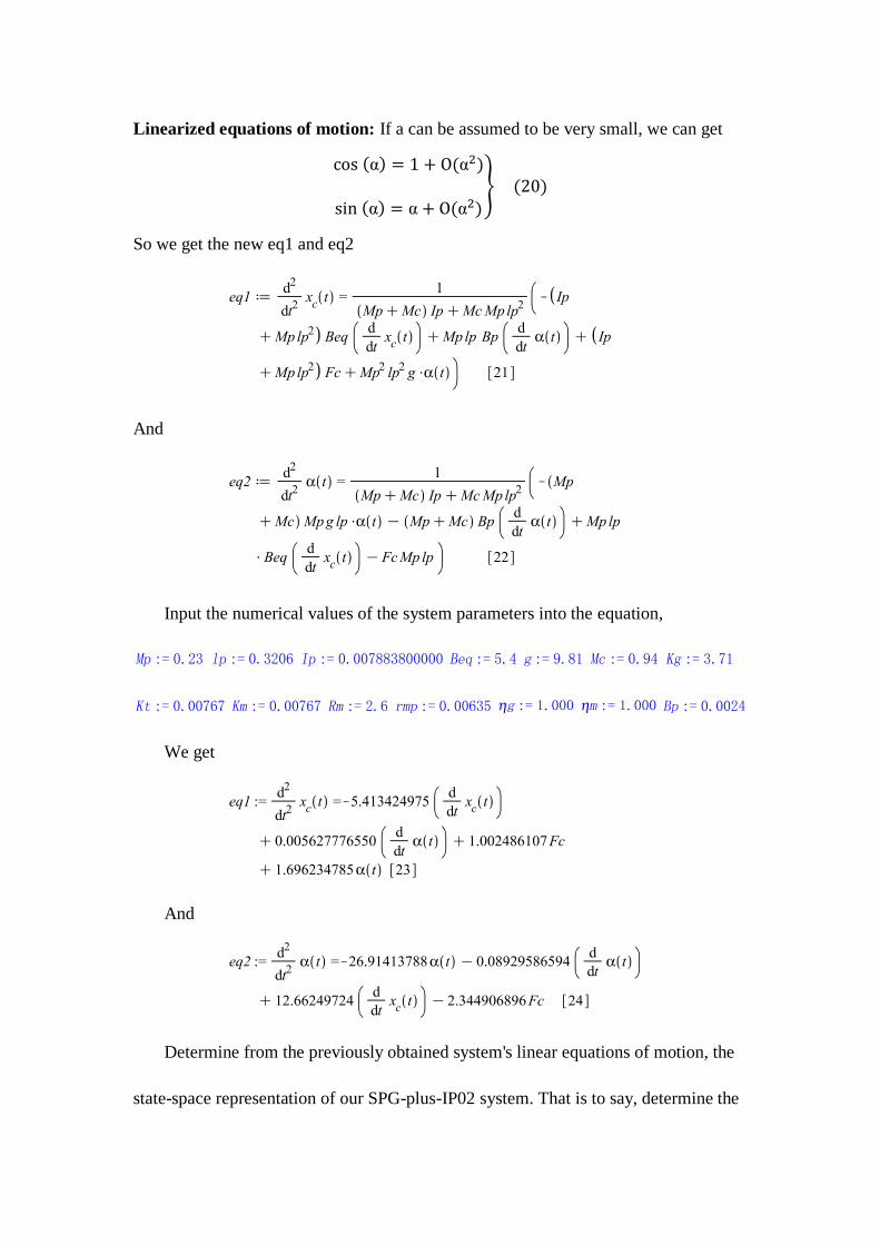
Linearized equations of motion: If a can be assumed to be very small, we can get

cos (α) = 1 + O(α2)

sin (α) = α + O(α2)} (20)

So we get the new eq1 and eq2

And

Input the numerical values of the system parameters into the equation,

We get

And

Determine from the previously obtained system's linear equations of motion, the

state-space representation of our SPG-plus-IP02 system. That is to say, determine the

state-space matrices A and B verifying the following relationship:

Where X is the system's state vector. In practice, X is often chosen to include the

generalized coordinates as well as their first-order time derivatives. In our case, X is

defined such that its transpose is as follows

Also in Equation [25], the input U is set in a first time to be Fc, the linear cart

driving force. Thus we have:

Final, we get the matrix A and B

From the system's state-space representation previously found, evaluate the

matrices A and B in case the system's input U is equal to the cart's DC motor voltage,

as expressed below:

In order to transform the previous matrices A and B, it is reminded that the

driving force, Fc, generated by the DC motor and acting on the cart through the motor

pinion has already been determined in previous laboratories. As shown for example

in Equation [10], it can be expressed as:

We will get the new matrix A and B

The characteristic equation of the open-loop system can be expressed as shown

below:

det (sI −A ) =0 [30]

Where det() is the determinant function, s is the Laplace operator, and I the

identity matrix. Therefore, the system's open-loop poles can be seen as the

eigenvalues of the state-space matrix A.

We get the characteristic equation

And the four open loop poles is

The open-loop transfunction can be expressed as shown below:

Pole Placement Design

In order to meet the design specifications previously stated, our system's

closed-loop poles need to be placed judiciously. This section shows one methodology

to do so. From here on, let us name the system's closed-loop poles (a.k.a. eigenvalues)

as follows: p1, p2, p3, p4.

The pole placement method used in this laboratory consists of locating a

dominating pair of complex and conjugate poles, p1 and p2 as illustrated in Figure 2

below, that satisfy the desired damping (i.e. PO) and bandwidth (i.e. ts) requirements.

The remaining closed-loop poles, here p3 and p4, are then assigned on the real axis to

the left of this pair, as seen in Figure 2. The dominating pair of poles p1 and p2, as

shown in Figure 2, can be expressed by the following equations:

p1=-ζωn + jβωn and p2=-ζωn − jβωn [33]

Where â is defined as:

β = √1 − ζ2 [34]

Since:

ζ= cos (φ) and β=sin (φ) [35]

Figure 2 Closed-Loop Pole Locations in the S-Plane

For our application, the suspended pendulum response performance should

satisfy the following design requirements:

1.The Percent Overshoot (PO) of the pendulum tip response along the x-coordinate,

xt, should be less than 5%, i.e.:

PO ≤ 5 %

2. The 2% settling time of the pendulum tip response along the x-coordinate, xt,

should be less than 2.2 seconds, i.e.:

ts≤2.2 [s]

Our group chooses overshoot as 1%, and it is less than 5%. The settling time is

equal to 2.2 seconds.

From the equation [36]

We get the ζ ,

And ts ,

So the characteristic equation

The solution is

40892958659.077353568.3091413788.260

500056277765.015619056.13696234785.10

1000

0100

A

0 4 1 5 4 8 5 8 6.4

7 2 7 8 2 8 2 1 9.1

0

0

B

0001C

0

0

0

0

D

From A, B, C, and D, we can find matrix Co, and we can identity if the system is

controllable and observable from matrix Co.

7.62325962.00535.0004.0

3.7648-2928.00228.00017.0

5962.00535.0004.00

2928.00228.00017.00

,,, 32 BABAABBCo

By using Matlab, we can find this matrix is rank 4, so it is controllable. We also

find

0000

0000

0000

0001

Do so, it is not observable.

Matlab Simulation of the Pole-Placement-Based

Controller

Matlab simulation from the previous derivation, we can get matrix A, B, C, and D

as following

A=

40892958659.077353568.3091413788.260

500056277765.015619056.13696234785.10

1000

0100

B=

041548586.4

727828219.1

0

0

C= 0001

D=

0

0

0

0

By using Matlab command “ss2zp”, we can get pole-zero locations of the SISO

system previously determined

i

iZ

7901.40381.0

7901.40381.0

i

iP

8352.41747.0

8352.41747.0

8960.12

0

K=1.7278

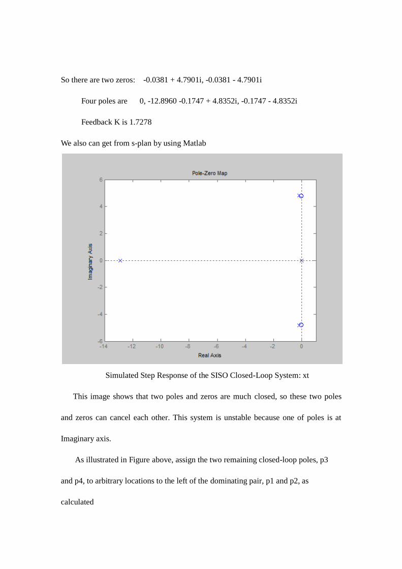
So there are two zeros: -0.0381 + 4.7901i, -0.0381 - 4.7901i

Four poles are 0, -12.8960 -0.1747 + 4.8352i, -0.1747 - 4.8352i

Feedback K is 1.7278

We also can get from s-plan by using Matlab

Simulated Step Response of the SISO Closed-Loop System: xt

This image shows that two poles and zeros are much closed, so these two poles

and zeros can cancel each other. This system is unstable because one of poles is at

Imaginary axis.

As illustrated in Figure above, assign the two remaining closed-loop poles, p3

and p4, to arbitrary locations to the left of the dominating pair, p1 and p2, as

calculated

The last p3 and p4 may be on the real axis since the desired damping requirement

should already be achieved by the designed p1 and p2.

p1= -1.818181819+1.2403663037i p2= -1.818181819-1.2403663037i

p3= -20 p4= -40

From these poles we can calculate the state-feedback gain vector, K, required

obtaining the four closed-loop pole locations.

6405.187661.720632.2027470.97 K

K1=97.7470

K2= -202.0632

K3=72.7661

K4=18.6405

In order to check my result, calculate the closed-loop poles of the obtained

state-feedback system. Firstly, we calculated the closed-loop state-space matrix can be

expressed as follows: A-B*K, then determine the eigenvalues of this matrix.

2472.758614.3245625.8430494.395

2020.328836.1388268.3508901.168

1000

0100

* KBA

From the matrix A-B*K, we attain poles below P1, P2, P3, and P4.

P1=-1.8182+1.2404i P2=-1.8182-1.2404i

P3=-20 P4=-40

We first assume p1, p2, p3 and p4, and get K from them by calculation in Matlab.

Then, we calculate P1, P2, P3, and P4 from the K. Finally, we find the P1, P2, P3, and

P4 match to p1, p2, p3 and p4 we assume before.

We also can get the closed-loop pole-zero location of the SISO system in the S-plane

from Matlab.

This image figure out the location of P1, P2, P3, and P4 we get from K. We can

find their S-plane from Matlab; and we can see the difference between the location of

P1, P2, P3, P4 and p1, p2, p3, p4.

006413.01C

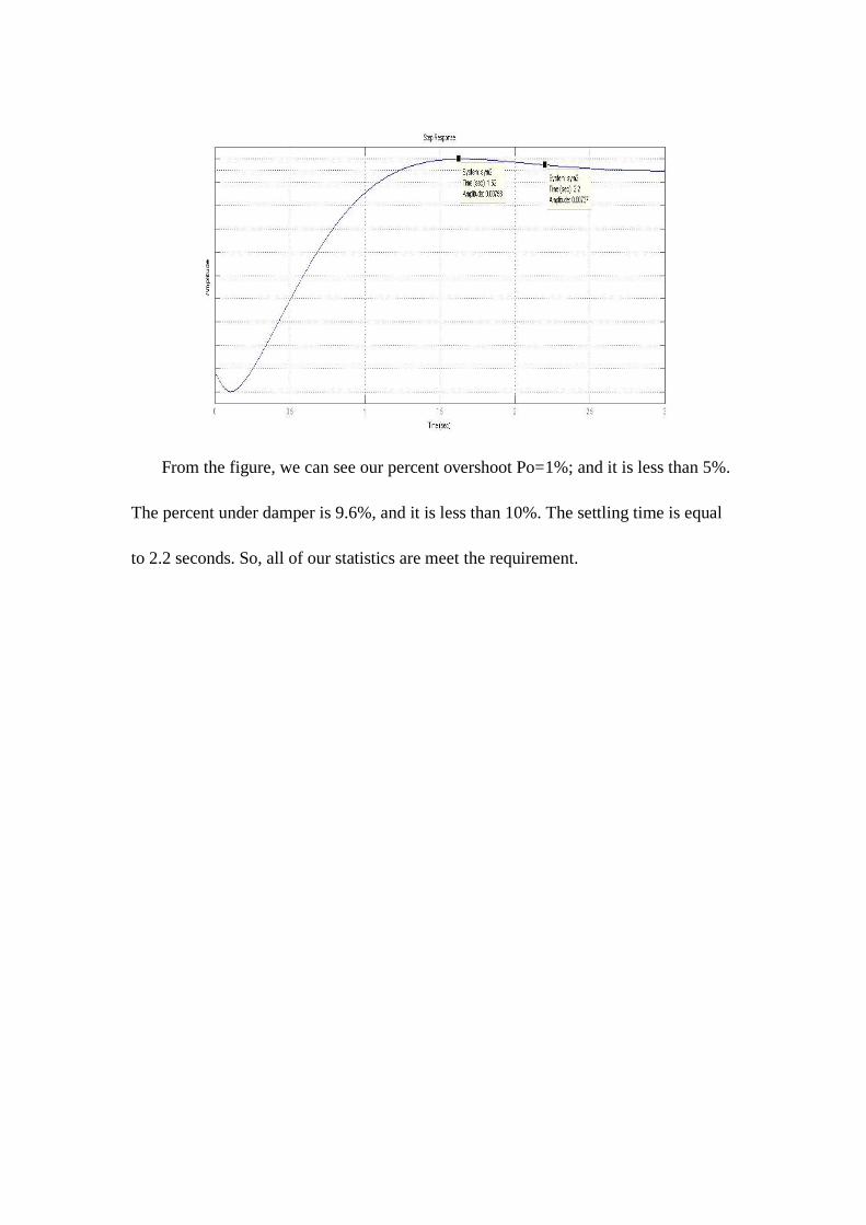
From the figure, we can see our percent overshoot Po=1%; and it is less than 5%.

The percent under damper is 9.6%, and it is less than 10%. The settling time is equal

to 2.2 seconds. So, all of our statistics are meet the requirement.

Simulink Simulation and Design of the

Pole-Placement-Based Controller

Simulink:

Step 1.Open the Simulink model file q_spg_pp_ip02. We obtain a diagram shown

in Figure 3. The model has 2 parallel and independent control loops: one runs a pure

simulation of the state-feedback-controller-plus-SPG-plus-IP02 system, using the

plant's state-space representation. Since full-state feedback is used, ensure that the C

state-space matrix is a 4-by-4 identity matrix; so C=eye(4). The other loop directly

interfaces with your hardware and runs your actual suspended pendulum mounted in

front of your IP02 linear servo plant. Open both subsystems to get a better idea of

their composing blocks as well as take note of the I/O connections.

Figure 3 Iinterfaces to the IP02 Plant

Interface to the actual SPG+IP02 System

And from previous state-space matrixs, we get:

A=

40892958659.077353568.3091413788.260

500056277765.015619056.13696234785.10

1000

0100

B=

041548586.4

727828219.1

0

0

C=

1000

0100

0010

0001

D=

0

0

0

0

Step 2. Check that the position set point generated for the cart and pendulum tip

x-coordinate to follow is a square wave of amplitude 30 mm and frequency 0.1 Hz.

Lastly, set the model sampling time to 1 ms, i.e. Ts = 10−3 s.

Step 3.Configure DAQ: Double-click on the HIL Initialize block inside the

SPG+IP02Actual Plant\IP02 subsystem and ensure it is configured for the DAQ

device that is installed in the system.

Step 4.Ensure that your feedback gain vector K satisfying the system

specifications .

K can be re-calculated in the Matlab workspace using the following command line:

>> K = place( A, B, [ p1 p2 p3 p4 ] )

Step 5. build the real-time code corresponding to our diagram

Step 6.Single Pendulum Gantry starting procedure

Step 7.Position the IP02 cart around the mid-track position and wait for the

suspended pendulum to come to complete rest.

Step 8.Start the real-time controller

Step 9.Open the Scopes/Pend Tip Pos (mm) sink. For more insight on the actual

system's behavior, also open the two sinks named Scopes/xc (mm) and Scopes/Pend

Angle (deg). Finally, check the system's control effort with regard to saturation, as

mentioned in the design specifications. Do so by opening the V Command (V) scope

located in the subsystem SPG + IP02: Actual Plant\IP02. On the Pend Tip Pos (mm)

scope, and monitor on-line, as the cart and pendulum move, the actual pendulum end

position as it tracks the re-defined reference input, and compare it to the simulation

result produced by the SPG-plus-IP02 state-space model. Such a response is shown as

below.

Step 10.Analyze the system response at this point, as shown on the Pend Tip Pos

(mm) scope, in terms of PO, ts, and steady-state error. by observing the Scopes/xc

(mm) and Scopes/Pend Angle (deg) scopes, showing. Also the corresponding control

effort spent, by monitoring the V Command (V) scope.

Step 11. refining your two real poles' positions, p3 and p4. Re-calculate (using the

Matlab 'place' function) the gain vector K and to apply it to the real-time code.

The effect of the P3 and P4.

We change different combination of pole 3 and pole 4, then we can calculate different

K.

1. For the Poles: p3=-20 p4=-40

-1.818181818+1.206796242i -1.818181818-1.206796242i -20 -40

Use Matlab we can get feedback vector K

we get Pend tip position , Pending angle, Xc and Vm.

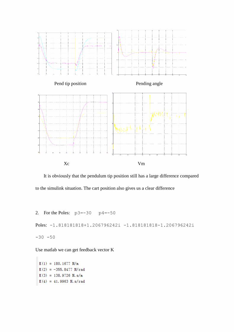
Pend tip position Pending angle

Xc Vm

It is obviously that the pendulum tip position still has a large difference compared

to the simulink situation. The cart position also gives us a clear difference

2. For the Poles: p3=-30 p4=-50

Poles: -1.818181818+1.206796242i -1.818181818-1.206796242i

-30 -50

Use matlab we can get feedback vector K

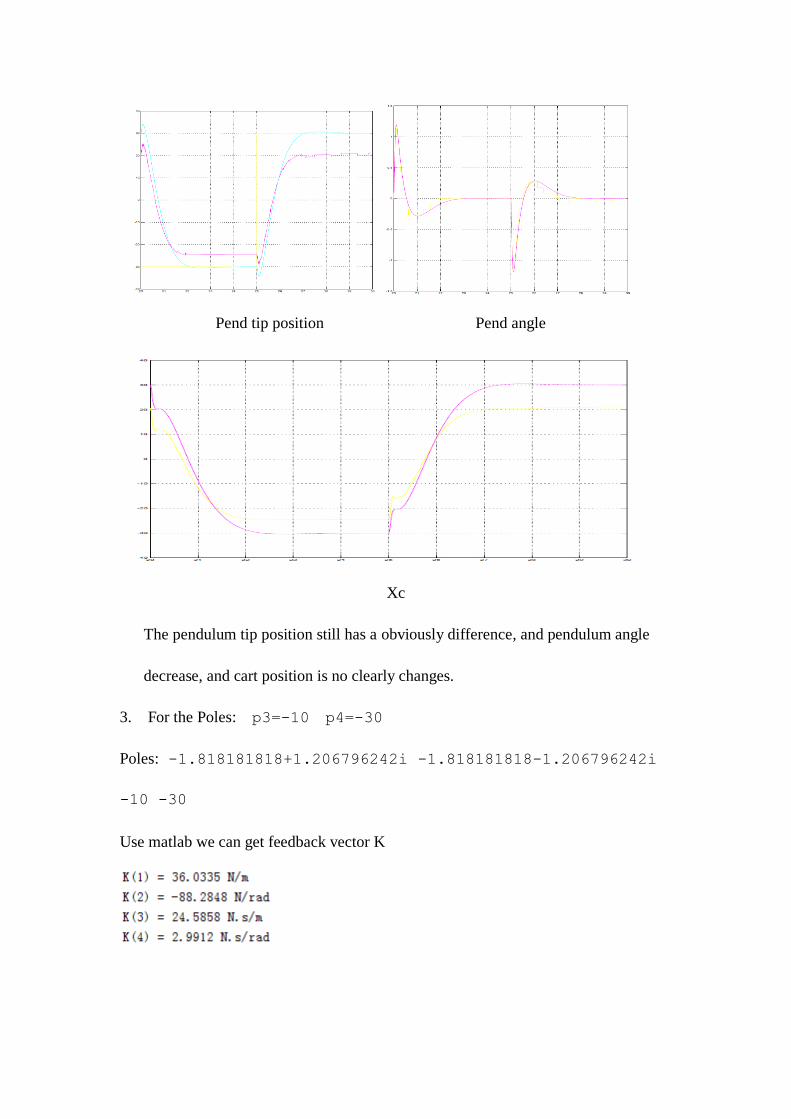
Pend tip position Pend angle

Xc

The pendulum tip position still has a obviously difference, and pendulum angle

decrease, and cart position is no clearly changes.

3. For the Poles: p3=-10 p4=-30

Poles: -1.818181818+1.206796242i -1.818181818-1.206796242i

-10 -30

Use matlab we can get feedback vector K

pend tip position pend angle

xc

The pendulum tip position has a huger distance compared the simulink. The

pendulum angle also increase obviously, the cart position still has no difference.

Compared different combination poles, it is obviously to conclude that at a

certain range, the poles is more big, the pendulum position is more close the simulink

position. But the pendulum angle is less and less. The cart position is very closed.

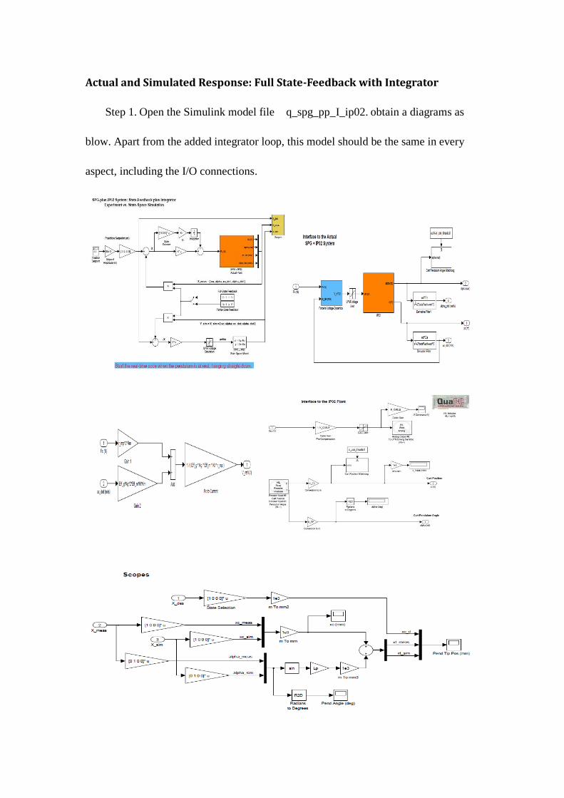
Actual and Simulated Response: Full State-Feedback with Integrator

Step 1. Open the Simulink model file q_spg_pp_I_ip02. obtain a diagrams as

blow. Apart from the added integrator loop, this model should be the same in every

aspect, including the I/O connections.

Step 2.The integral gain is named Ki. First set Ki to zero in the Matlab

workspace. Then, compile and run your state-feedback controller with integral action

on xc . Re-open the previous Scopes of interest. Monitoring the system actual

response plotted in the Scopes/Pend Tip Pos (mm) Scope, change the Ki to eliminate

the steady-state error.

(Actual and Simulated Response: Full State-Feedback with Integrator. In the top

plot, the green dash-dot line is the setpoint, the blue dot trace is the simulation, and

the solid red trace is the measured pendulum position. The bottom plot is the motor

input voltage.)

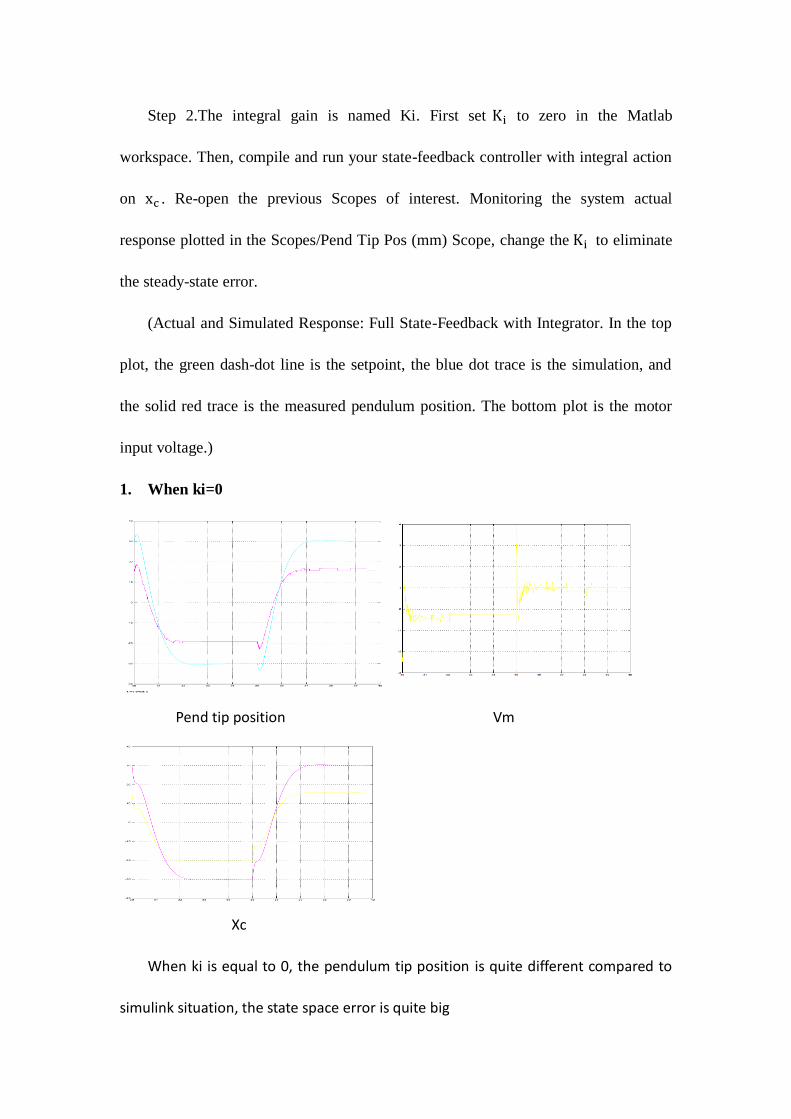
1. When ki=0

Pend tip position Vm

Xc

When ki is equal to 0, the pendulum tip position is quite different compared to

simulink situation, the state space error is quite big

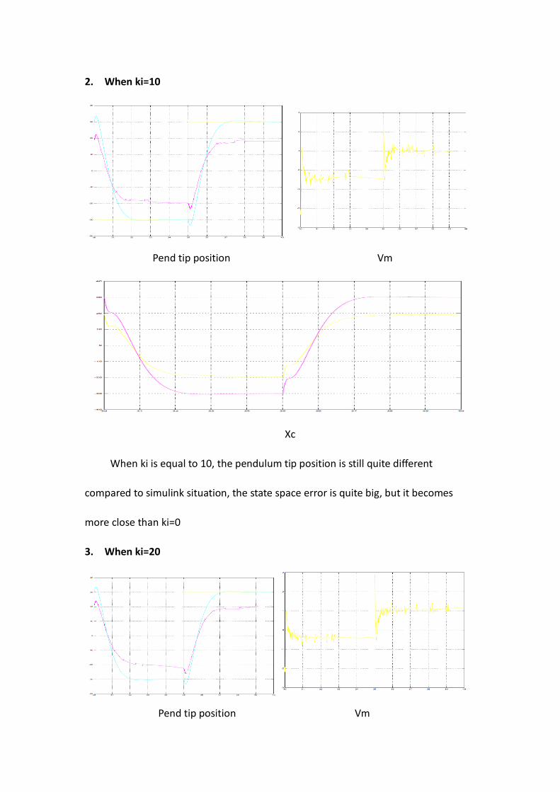
2. When ki=10

Pend tip position Vm

Xc

When ki is equal to 10, the pendulum tip position is still quite different

compared to simulink situation, the state space error is quite big, but it becomes

more close than ki=0

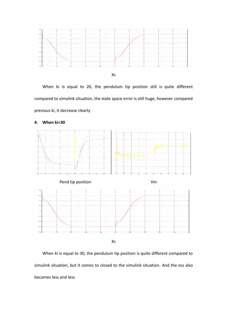
3. When ki=20

Pend tip position Vm

Xc

When ki is equal to 20, the pendulum tip position still is quite different

compared to simulink situation, the state space error is still huge, however compared

previous ki, it decrease clearly

4. When ki=30

Pend tip position Vm

Xc

When ki is equal to 30, the pendulum tip position is quite different compared to

simulink situation, but it comes to closed to the simulink situation. And the ess also

becames less and less

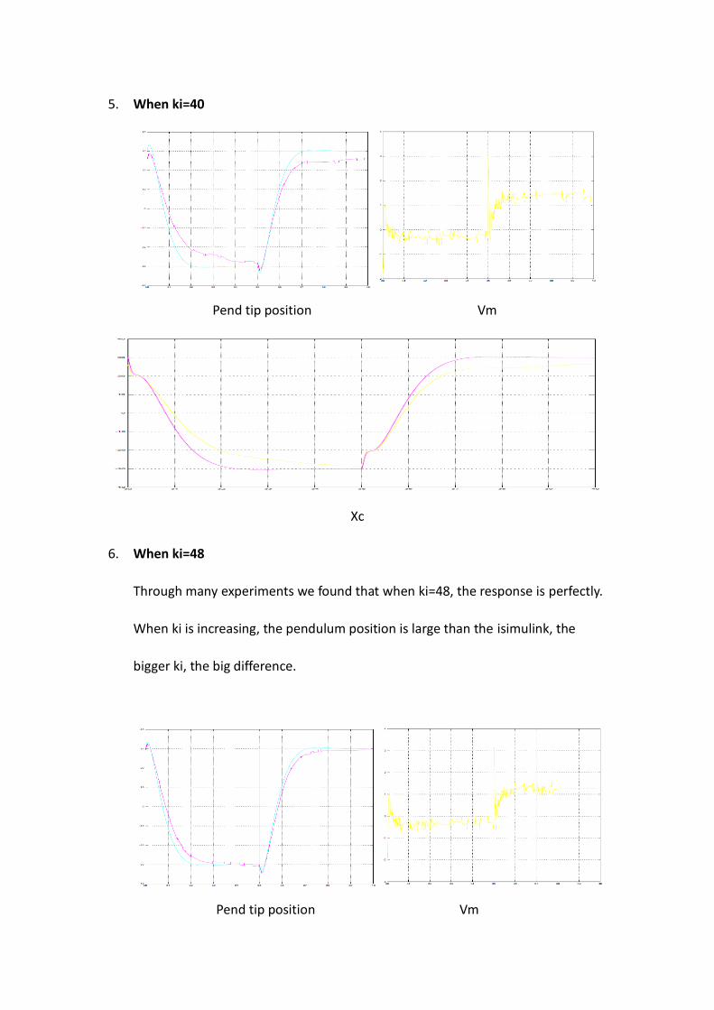
5. When ki=40

Pend tip position Vm

Xc

6. When ki=48

Through many experiments we found that when ki=48, the response is perfectly.

When ki is increasing, the pendulum position is large than the isimulink, the

bigger ki, the big difference.

Pend tip position Vm

Xc Pend angle

It is obvious that the pendulum tip position is almost the same compare to Simulink,

the input Vm are also not saturation. The cat position is also the closed.

According to the experiment, we should change the different combination of the third

and forth poles. We still choose the previous poles combination

Change p3,p4 into -30 -50

We get the response as blow.

Pend tip position Vm

Xc

It is obviously that when we change the poles, the pendulum tip position begun

to make some changes. It is not so closed to simulink line, and the input Vm has a

more seriously vibration.

When p3,p4 =-10 -30

Pend tip position Vm

Xc

When choose another combination of poles, it is easily found that the pendulum

position is quite difference, the error became bigger and bigger, the input vm increase

more obviously.

According to the experiment required, we should, on a side note, double-click on the

manual switch located around the centre of our diagram. This should move the switch

from the "up" to the "down" position. In the down position, some of the fed-back state

vector elements (i.e. states) are multiplied by zero, therefore canceling their feedback:

your closed-loop becomes then with partial-state feedback

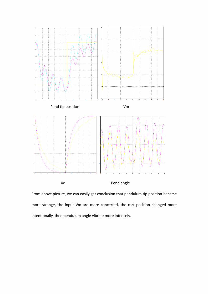
Pend tip position Vm

Xc Pend angle

From above picture, we can easily get conclusion that pendulum tip position became

more strange, the input Vm are more concerted, the cart position changed more

intentionally, then pendulum angle vibrate more intensely.