I Single-molecule Nanoscopy of RNA Polymerase II Transcription at a Single Gene in Live Cells by Ankun Dong Submitted in partial fulfillment of the requirements for the Degree of Doctor of Philosophy in the Department of Physics at Brown University Providence, Rhode Island May 2017

Welcome message from author
This document is posted to help you gain knowledge. Please leave a comment to let me know what you think about it! Share it to your friends and learn new things together.
Transcript

I
Single-molecule Nanoscopy of RNA
Polymerase II Transcription at a Single
Gene in Live Cells
by
Ankun Dong
Submitted in partial fulfillment of the requirements
for the Degree of Doctor of Philosophy in the
Department of Physics at Brown University
Providence, Rhode Island
May 2017

II
@Copyright 2017 by Ankun Dong

III
This dissertation by Ankun Dong is accepted in its present form
by the Department of Physics as satisfying the
dissertation requirement for the degree of Doctor of Philosophy.
Date_____________ _________________________________
Professor Xinsheng Sean Ling, Advisor
Recommended to the Graduate Council
Date_____________ _________________________________
Professor J. Michael Kosterlitz, Reader
Date_____________ _________________________________
Professor Gerald J.Diebold, Reader
Approved by the Graduate Council
Date_____________ _________________________________
Andrew G. Campbell
Dean of the Graduate School

IV
Acknowledgements
Life is a journey, the six-year PhD study will definitely be an extremely valuable
experience for me.
Firstly, I would like to thank Dr. Alexandros Pertsinidis for providing the
opportunity to conduct the cutting edge research at Memorial Sloan Kettering Cancer
Center. I am grateful for the financial support and academic guidance. I also thank
him for initiating me into the cult of single molecule imaging, and for answering my
questions - usually in 10 seconds or less. I admire his tireless pursuit of knowledge
and full commitment in science even at the expense of sleep and repast.
Secondly, I am forever indebted to my advisor at Brown University Professor
Xinsheng Sean Ling for his professional advice and valuable suggestions. His
enthusiasm for science, how he helped other people and how he loved his family, have
made huge impact on me and set me a good example. I still remember his
encouraging and incentive conversations with me in his office.
Thirdly, I thank Professor John Michael Kosterlitz for taking interests in my
research and listening to my presentation right after his medical procedure on Mar,
27th
, 2017. I thank Prof Gerald. J. Diebold for inviting me to give a talk in the
Department of Chemistry as a practice of my thesis defense. It is a great honor for

V
me to have them on my defense committees. I thank them for reading my Ph.D.
dissertation and providing valuable advices.
Then I thank all my friends around for their companionship, the sharing and
mental support.
Last but not least, I am especially grateful to my parents. They supported me
when I was under a mountain (either literally or figuratively) and shared with me all
the happy moments.

VI
Abstract of “Single-molecule Nanoscopy of RNA Polymerase II Transcription at a
Single Gene in Live Cells” by Ankun Dong, Ph.D., Brown University, May 2017
Single-molecule approaches enable us to follow the movement, interactions and
conformational dynamics of individual molecules in real-time, thus providing novel
insights in complex biochemical systems that have remained masked in the ensemble
averaging of traditional bulk biochemical approaches. Recent advances in
single-molecule tracking, fluorescence spectroscopy and subdiffraction optical
microscopy have unveiled unprecedented views of molecular processes in live cells.
To extract quantitative information from individual molecules in the high background
noise, these techniques are often based on in vitro reconstituted systems with either
surface-immobilized or freely-diffusing biomolecules in dilute conditions. Live cell,
real-time imaging, tracking and counting biomolecules in their native, crowded
intracellular environment currently remain an extremely challenging task.
Based on the numerical simulation, I built the real time tracking 3D STED nanoscopy
enabling single molecule detection. With the new technique, I perform
oligo-nucleotide hybridization detection experiment in vitro as well as study the
mechanism of RNA Polymerase II transcription in living cells at single molecule level.
Basically, I reveal the accumulation of Pol II molecules and quantified nearly 10 Pol
II molecules in the cluster during active transcription at a tagged mini-gene in the
native environment. In addition, mini-gene transcription does not involve transient Pol

VII
II clustering at pre-initiation by kinetic analysis enabled by target-locking over
multiple transcription rounds, arguing against the persistence of accumulated Pol IIs
in the absence of transcription or extensive Pol II recycling-related spatial
compartmentalization. What’s more, I find that single Pol II molecules are
stochastically recruited from the nucleoplasm, enter into productive elongation and
are predominantly released instead of recycled upon termination. The results set up a
quantitative framework for investigating Pol II dynamics at single genes at single
molecule level, and also demonstrate that the potential and powerful use of real time
tracking 3D STED nanoscopy in elucidating the complex biological mechanisms in
vivo.

VIII
List of Acronyms
FWHM Full Width with Half Maximum
STED Stimulated Emission Depletion
TIR Total Internal Reflection
SIM Structured Illumination Microscopy
STORM Stochastic Optical Reconstruction Microscopy
NSOM Near-field Scanning Optical Microscopy
Epi Epifluorescence
PALM Photoactivated Localization Microscopy
pcPALM Pair-correlation PALM
GFP Green Fluorescent Protein
mRNA message RNA
Pol II polymerase II
NTP Nucleoside triphosphate
TBP TATA-binding protein
TFB transcription factor B
TFE Transcription factor E
TFIIA Transcription factor II A
TFIIB Transcription factor IIB
TFIID Transcription factor IID
TFIIE Transcription factor IIE
IX
TFIIF Transcription factor IIF
TFIIH Transcription factor IIH
CTD C-terminal domain
BrUTP bromouridine triphosphate
CHO Chinese hamster ovary
TMR Tetramethylrhodamine
RPB1 RNA polymerase II large subunit
NSF N-ethylmaleimide sensitive fusion proteins
SNAP Soluble NSF Attachment Protein
SiR Silicon Rhodamine
3D 3 dimensional
PSF Point Spread Function
PBS Polarized Beam Splitter
SLM Spatial Light Modulator
LCOS-SLM Liquid Crystal on Silicon-Spatial Light Modulator
APD Avalanche photodiode
CCD charge coupled device
PMT Photomultiplier
BNC Bayonet Neill–Concelman
PEG Poly-ethylene-glycol
CW Continuous Wave
OPO Optical Parametric Oscillator
X
SNR Signal to Noise Ratio
BSA Bovine serum albumin
FRET Förster resonance energy transfer
ROI Region of Interest
KD Dissociation constant
CMV-IE Cytomegalovirus immediate-early
BFP Blue Fluorescent Protein
FCS Fluorescence correlation spectroscopy
PID Proportional–integral–derivative
SD Standard Deviation
fps Frame per second
DMSO Dimethyl sulfoxide

Contents
1. Introduction 1
1.1 Super Resolution Fluorescent microscope in life science 2
1.1.1 Introduction 2
1.1.2 Near field 3
1.1.3 TIR 5
1.1.4 Confocal 6
1.1.5 Two Photon Excitation 8
1.1.6 SIM 11
1.1.7 STED 13
1.1.8 TORM/PALM 15
1.1.9 Summary 16
1.2 Gene Expression 18
1.2.1 Mechanism: Transcription, RNA processing, Non-coding RNA
maturation, RNA export, Translation, Folding, Translocation, Protein
transport
18
1.2.2 Transcription of Eukaryotic Protein-Coding Genes: Initiation,
Promoter escape, Elon1gation, Termination
19
1.2.3 RNA Polymerase II in transcription 19
1.2.3.1 RNA Polymerase II and initiation cofactors 20
1.2.3.2 RNA Polymerase II and elongation cofactors 21
1.2.4 Polymerase II Clustering 21
2. Simulation of single molecule detection using STED 30
2.1 Numerical Simulation Theory 31
2.2 Excitation beam 32
2.3 Vortex doughnut 35
2.4 Z doughnut 36
2.4.1 Central intensity with different phase modulation 36
2.4.2 Z doughnut with the optimal phase modulation 38
2.5 Emission of a dipole 38
2.6 Resolution with different combinations of xy and z doughnut 40
3. Setup 42
3.1 Schematic 43
3.2 Setup components(excitation lasers ,STED lasers, Objectives, Filters,
Detectors, piezo Stage, vortex plate, SLM)
43
3.3 Align the setup 45
3.3.1 Coarse alignment based on the reflected images on the CCD camera 45
3.3.2 Calibrate the beams using gold nanoparticle (PMT used) 46
3.3.2.1 xz scanning 46

3.3.2.2 xy scanning 47
3.3.3 Quarter wave plate adjustment 48
3.3.4 Optimal collar position for Silicon oil and regular oil objective 48
3.3.5 Optimize z doughnut by changing the collimation and phase
modulation
49
3.3.6 Overlap all the beams 50
3.4 Resolution vs power 50
3.4.1 Immobile molecules sample preparation 50
3.4.2 Later resolution vs STED power 51
3.4.3 Axial resolution vs STED power 53
3.5 Time gating 55
3.5.1 Take data with APD detector and Picoharp (T2 mode and T3 mode) 55
3.5.2 Lifetime of the fluorescence 56
3.5.3 STED changes the lifetime 57
3.5.4 Time gating improves the resolution 58
3.6 CW laser vs pulsed mode laser 59
3.6.1 Pulsed mode properties 59
3.6.2 Optimize the phase to achieve the highest depletion 60
3.6.3 Compare the two modes 60
4. STED improves SNR and enable single molecule
detection in vivo
61
4.1 STED principle 62
4.2 The reversible depletion of STED on single fluorophore 63
4.3. The general Background properties 64
4.3.1 Closed system 64
4.3.2 Open system 65
4.4 The STED depletion in the Atto647N solution at different concentration 65
4.4.1 Background and noise from the solution and surface 65
4.4.2 Background and noise with different excitation power 66
4.4.3 Background and noise with different excitation power Background
and noise with and without STED of the Atto647N solution at different
concentration
67
4.5 Detection of immobile single molecules at elevated concentrations 72
4.5.1 Experiment design 72
4.5.2 Cy3-Atto647N duplex preparation 73
4.5.3 Map the yellow channel and red channel 73
4.5.4 Scan the regions with yellow, red and red with sted at elevated
concentrations (100nM, 300nM, 600nM)
74
4.5.5 Construct and compare the images 75
4.5.6 Quantify the SNR with and without STED (The distribution of the
signal from the Cy3 colocalized regions and random regions)
77
4.6 DNA hybridization on off binding detection 78

4.6.1 Experiment design 78
4.6.2 The on off rate optimization 79
4.6.2.1 Kd of different oligos (10nt, 9nt, 8nt) 79
4.6.2.2 Adjust the Kd with NaCl at different concentrations 81
4.6.3 Map the yellow channel and red channel 81
4.6.4 Interlace the yellow laser and red laser 81
4.6.5 Take time traces with the interlaced yellow and red laser w/wo STED 82
4.6.6 Data analysis 82
4.6.6.1 Separate the direct red excitation and FRET traces 82
4.6.6.2 SNR of the direct excitation traces with/without STED 83
5. Single molecule detection for RNA Polymerase II
transcription
85
5.1 Mini gene 86
5.2 Sample preparation (Rpb1 and Rpb9) 87
5.3 Background and noise in living Rpb9 cells 88
5.3.1 FCS experiment 88
5.3.2 Background and noise reduction with STED 88
5.4 Pol II accumulates at sites of active nascent transcription(wide field
imaging)
91
5.5 Studying the Pol II using STED setup (methods) 92
5.5.1 STED alignment 92
5.5.2 Quad-view camera registration 93
5.5.3 GFP tracking 94
5.5.4 Data analysis (extracting the time traces) 96
5.6 Colocalization of Pol II and mRNA 96
5.6.1 Check the Colocalization using the initial images with the
background subtracted from the quad-view camera
96
5.6.2 Check the Colocalization by direct 3D scanning images 98
5.6.2.1 Find the GFP spots and roughly center the spots 98
5.6.2.2 3D real time imaging using FPGA 98
5.7 Bleaching traces for counting Pol II numbers 100
5.7.1 Calibrate the step size of the bleaching time traces using less stained
sample
101
5.7.2 Count Pol II numbers using fully stained sample 103
5.7.3 Compare the bleaching traces with\without STED (2 fold SNR
improvement)
104
5.8 Quantification of Pol II at transcription sites 106
5.8.1 The initial peak of the traces at transcription sites and 536nm away 107
5.8.2 The decay time of the traces at transcription sites and 536nm away 108
5.8.3 The images of the Polymerase 0.536um away from transcription sites 109
5.8.4 The actual Pol II numbers involved in transcription 111
5.9 Size of the Pol II spots at transcription sites 112

5.9.1 Measure the sizes of the initial images with the background
subtracted from the quad-view camera referring to nanoparticle size
calibration
113
5.9.1.1 Calibrate the image sizes on the quad-view camera using
100,200,500nm nanoparticles without z tracking
114
5.9.1.2 Calibrate the image sizes on the quad-view camera using
100,200,500nm nanoparticles with z tracking
117
5.9.1.3 Compare the sizes of the Pol II images with that of the
nanoparticles
119
5.9.2 Check the sizes of the initial images with the background subtracted
from the quad-view camera with xy doughnut of different power
122
5.9.2.1 Resolution, Signal remaining with different power xy doughnut 123
5.9.2.2 Fit the size with calibrated data 123
5.9.3 Measure the Pol II sizes by 3D scanning 125
5.10 Dynamics of the Pol II transcription cycle at the CMV mini-gene 126
5.10.1 Pol II recovery experiment 126
5.10.1.1Bleaching the Pol II and retake the bleaching traces after certain
minutes
126
5.10.1.2 10-minute recovery time trace with low duty cycle excitation 128
5.10.1.3 3D scanning images before and after bleaching as well as after
10-minute recovery
130
5.10.2 SiR-Rpb1 FRAP experiments from wide field imaging 131
5.10.2.1 Take bleaching traces with time information recorded from
many cells using high excitation power
132
5.10.2.2 Take the 8-minute trace with low excitation power from each
cells
133
5.10.2.3 Data analysis and Conclusion 134
Bibliography 135

1
Chapter One
Introduction

2
1. Introduction
1.1 Super Resolution Fluorescent microscope in life science
1.1.1 Introduction
The 2014 Nobel Prize in Chemistry was awarded to Eric Betzig, W.E Moerner
and Stefan Hell for the development of super-resolved fluorescence microscopy.
Fluorescence microscopy has become an essential and powerful tool in biology. It
is widely used in imaging protein expression, localization, and activity in living cells.
Due to the diffraction limit, the resolution of conventional microscopy is
characterized by the excitation wavelength, first stated by Ernst Abbe in 1873 [1]. The
resolution of the microscopy is usually denoted by the full width at half
maximum (FWHM) of the point spread function, and a typical wide field microscope
with a high numerical aperture [2] reaches a resolution of roughly half the excitation
wavelength. This makes sharp point-like objects to appear blurry under the
microscope and many fine cellular structures unresolvable.
In biological systems, people often need to deal with densely packed, brightly
labeled diffraction limited structures. Over the past several decades, people have
developed several super-resolution techniques for breaking the diffraction barrier. In
this chapter, I will briefly summarize near-field super-resolution microscopy. TIR,
Confocal, Two Photon excitation, SIM, STED and STORM microscopy which are
now most widely used have great impact on biological research. I am not going into
particularly some other microscopy that are developed from these ones.
3
1.1.2 Near field
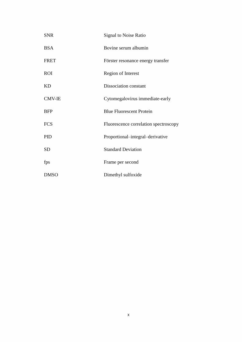
Near-field scanning optical microscopy (NSOM), by its name, breaks the far
field resolution limit by taking advantage of the properties of evanescent waves. As
the diffraction limit is for the far field description, in the evanescent region, which is
near the surface of the object, the intensities drop off exponentially with distance from
the object [3].
Figure 1.1: Diagram illustrating near field optics
To realize this, the detector is placed very close to the sample, and actually the
distance between the detector and the specimen need to be much smaller than the
excitation wavelength λ. In this way, the resolution of the image is limited by the size
of the aperture instead of the wavelength of the excitation beam. NSOM can be easily
used to study different properties, such as refractive index, chemical structure and
local stress. Dynamic properties can also be studied at a sub-wavelength scale. In
particular, lateral resolution of 20 nm and vertical resolution of 2–5 nm have been
demonstrated. Step and terrace structure has been observed in the 1mm by 1 mm area
on the cleaved surface of KCl–KBr solid-solution single crystal using NSOM. In the
experiment, a small sphere probe of 500 nm diameter is used [4].

4
Figure 1.2: The magnified SNOM image of the small area in a river pattern existing on the cleaved surface of KCl–KBr solid-solution single crystal [4].
As the detector is very close to the sample, NSOM has some limitations: The
working distance need be very low, so this technique could only work for surface
study. It is not conducive for studying soft materials. What‟s more, long scan time is
needed for large sample areas for high resolution imaging.

5
1.1.3 TIR
In molecular biology, in the case of studying a large
number of molecular events in cellular surfaces such
as cell adhesion, the surfaces attached molecules as well
as much more non-bound molecules in the medium will
be excited using conventional microscopy. The
non-bound molecules will lead to very high background
and make it changeling to observe the molecules bound
to the surface. A TIRFM uses an evanescent wave to
selectively illuminate and excite fluorophores in a
restricted region close to the glass-water interface,
making it a perfect method for the above surface
experiment.
Figure 1.4: Diagram showing the internal totally reflection
According to Snell‟s law [5],
where n1,n2 are the refractive index of the glass and water.
When is 90 degree,
θ1
θ2
n1
n2
Evanescent wave
range
Figure 1.3: Human skin fibroblasts labeled with dil and viewed at (a) TIRF, (b) Epi fluorescence of the same field. (c) Phase contrast of the same field [6].
6
= arcsin(n2/n1)
If , the incident beam will be totally reflected at the glass-water
interface. The electromagnetic field decays exponentially from the glass-water
interface, the penetration depth of nearly 100 nm into the medium is under the
diffraction limit.
Comparison of the labeled human skin fibroblasts images from TIRF, Epic
fluoresce and Phase contrast in Figure 1.3 [6] demonstrate that for TIRF only the
fluorophores near the surface would be excited, thus the TIRFM enables a selective
visualization of surface regions and have potential applications, including
visualization of the membrane and underlying cytoplasmic structures at cell-substrate
contacts, mapping of membrane topography, and visualization of reversibly bound
fluorescent ligands at membrane receptors.
1.1.4 Confocal
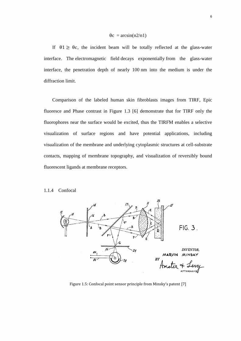
Figure 1.5: Confocal point sensor principle from Minsky's patent [7]

7
Confocal microscopy aims to overcome the limitations of traditional
wide-field fluorescence microscopes. In wide field microscopy, a large part of the
sample is illuminated at the same time and all the fluorescent light is collected.
Confocal microscopy increases the resolution and contrast of the images by adding
a spatial pinhole at the confocal plane of the lens before the detector to cut the
out-of-focus light. The first confocal scanning microscope was built by Marvin
Minsky in 1955, as seen in Figure 1.5 [7]. It enables the reconstruction of
three-dimensional structures from the obtained images by optical sectioning for a
thick object. Confocal laser scanning microscopes utilize multiple mirrors to scan the
laser across the sample or move the sample while keeping the beam. This technique is
widely used in life sciences, semiconductor inspection and materials science.
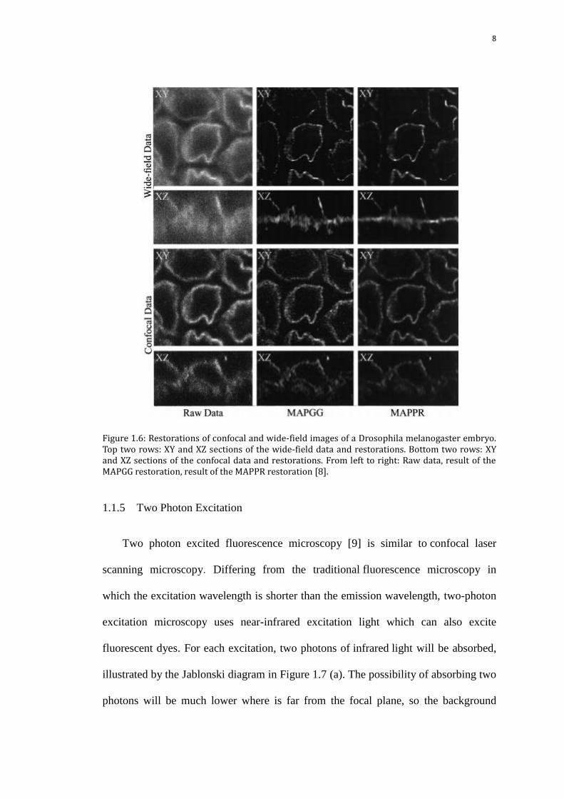
In Figure 1.6, restorations of confocal and wide-field images of a Drosophila
melanogaster embryo are compared. The confocal images show high resolution and
the images look more similar to the raw data [8].
8
Figure 1.6: Restorations of confocal and wide-field images of a Drosophila melanogaster embryo. Top two rows: XY and XZ sections of the wide-field data and restorations. Bottom two rows: XY and XZ sections of the confocal data and restorations. From left to right: Raw data, result of the MAPGG restoration, result of the MAPPR restoration [8].
1.1.5 Two Photon Excitation
Two photon excited fluorescence microscopy [9] is similar to confocal laser
scanning microscopy. Differing from the traditional fluorescence microscopy in
which the excitation wavelength is shorter than the emission wavelength, two-photon
excitation microscopy uses near-infrared excitation light which can also excite
fluorescent dyes. For each excitation, two photons of infrared light will be absorbed,
illustrated by the Jablonski diagram in Figure 1.7 (a). The possibility of absorbing two
photons will be much lower where is far from the focal plane, so the background
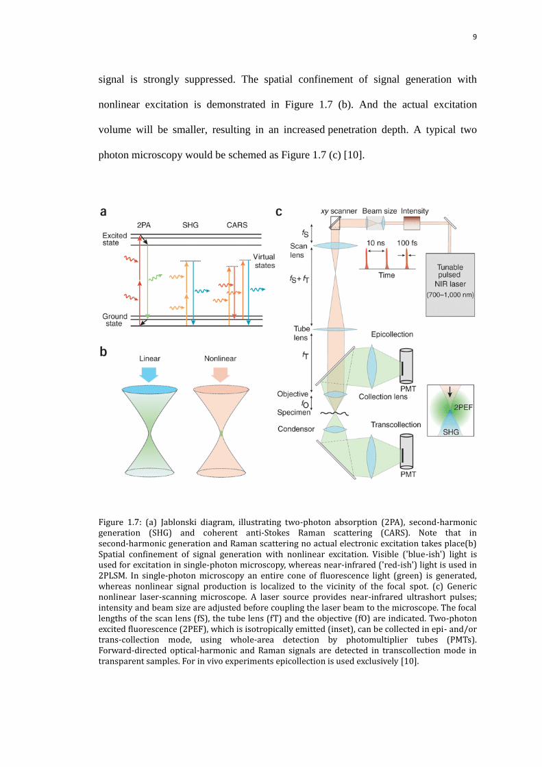
9
signal is strongly suppressed. The spatial confinement of signal generation with
nonlinear excitation is demonstrated in Figure 1.7 (b). And the actual excitation
volume will be smaller, resulting in an increased penetration depth. A typical two
photon microscopy would be schemed as Figure 1.7 (c) [10].
Figure 1.7: (a) Jablonski diagram, illustrating two-photon absorption (2PA), second-harmonic generation (SHG) and coherent anti-Stokes Raman scattering (CARS). Note that in second-harmonic generation and Raman scattering no actual electronic excitation takes place(b) Spatial confinement of signal generation with nonlinear excitation. Visible ('blue-ish') light is used for excitation in single-photon microscopy, whereas near-infrared ('red-ish') light is used in 2PLSM. In single-photon microscopy an entire cone of fluorescence light (green) is generated, whereas nonlinear signal production is localized to the vicinity of the focal spot. (c) Generic nonlinear laser-scanning microscope. A laser source provides near-infrared ultrashort pulses; intensity and beam size are adjusted before coupling the laser beam to the microscope. The focal lengths of the scan lens (fS), the tube lens (fT) and the objective (fO) are indicated. Two-photon excited fluorescence (2PEF), which is isotropically emitted (inset), can be collected in epi- and/or trans-collection mode, using whole-area detection by photomultiplier tubes (PMTs). Forward-directed optical-harmonic and Raman signals are detected in transcollection mode in transparent samples. For in vivo experiments epicollection is used exclusively [10].
10
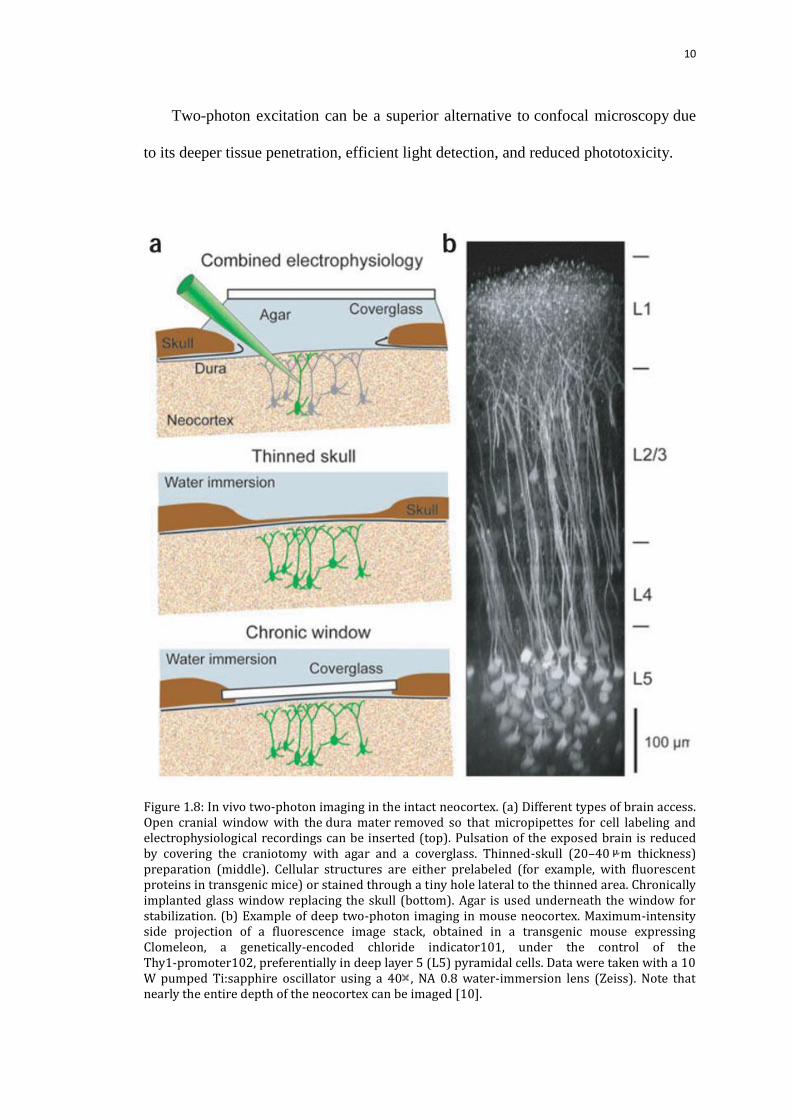
Two-photon excitation can be a superior alternative to confocal microscopy due
to its deeper tissue penetration, efficient light detection, and reduced phototoxicity.
Figure 1.8: In vivo two-photon imaging in the intact neocortex. (a) Different types of brain access. Open cranial window with the dura mater removed so that micropipettes for cell labeling and electrophysiological recordings can be inserted (top). Pulsation of the exposed brain is reduced by covering the craniotomy with agar and a coverglass. Thinned-skull (20–40 m thickness) preparation (middle). Cellular structures are either prelabeled (for example, with fluorescent proteins in transgenic mice) or stained through a tiny hole lateral to the thinned area. Chronically implanted glass window replacing the skull (bottom). Agar is used underneath the window for stabilization. (b) Example of deep two-photon imaging in mouse neocortex. Maximum-intensity side projection of a fluorescence image stack, obtained in a transgenic mouse expressing Clomeleon, a genetically-encoded chloride indicator101, under the control of the Thy1-promoter102, preferentially in deep layer 5 (L5) pyramidal cells. Data were taken with a 10 W pumped Ti:sapphire oscillator using a 40 , NA 0.8 water-immersion lens (Zeiss). Note that nearly the entire depth of the neocortex can be imaged [10].

11
The Two Photon Excitation microscopy has been used for high-resolution
imaging in various organs of living animals for its great advantages of imaging deep
within intact tissue. Figure 1.8 [10] demonstrates the cellular and subcellular imaging
in the intact brain.
1.1.6 SIM
Structured illumination is a wide field technique. Instead of the whole sample is
excited laterally, a grid pattern is generated through interference of diffraction orders
and superimposed on the sample, which cause normally inaccessible high-resolution
information to be encoded into the observed image. Most information for
reconstructing the image of a small object is mainly from the high-intensity
component. In reciprocal space from Fourier transformation, high-frequency
information can be extracted from the raw data to produce a reconstructed image
having a lateral resolution approximately twice that of diffraction-limited instruments
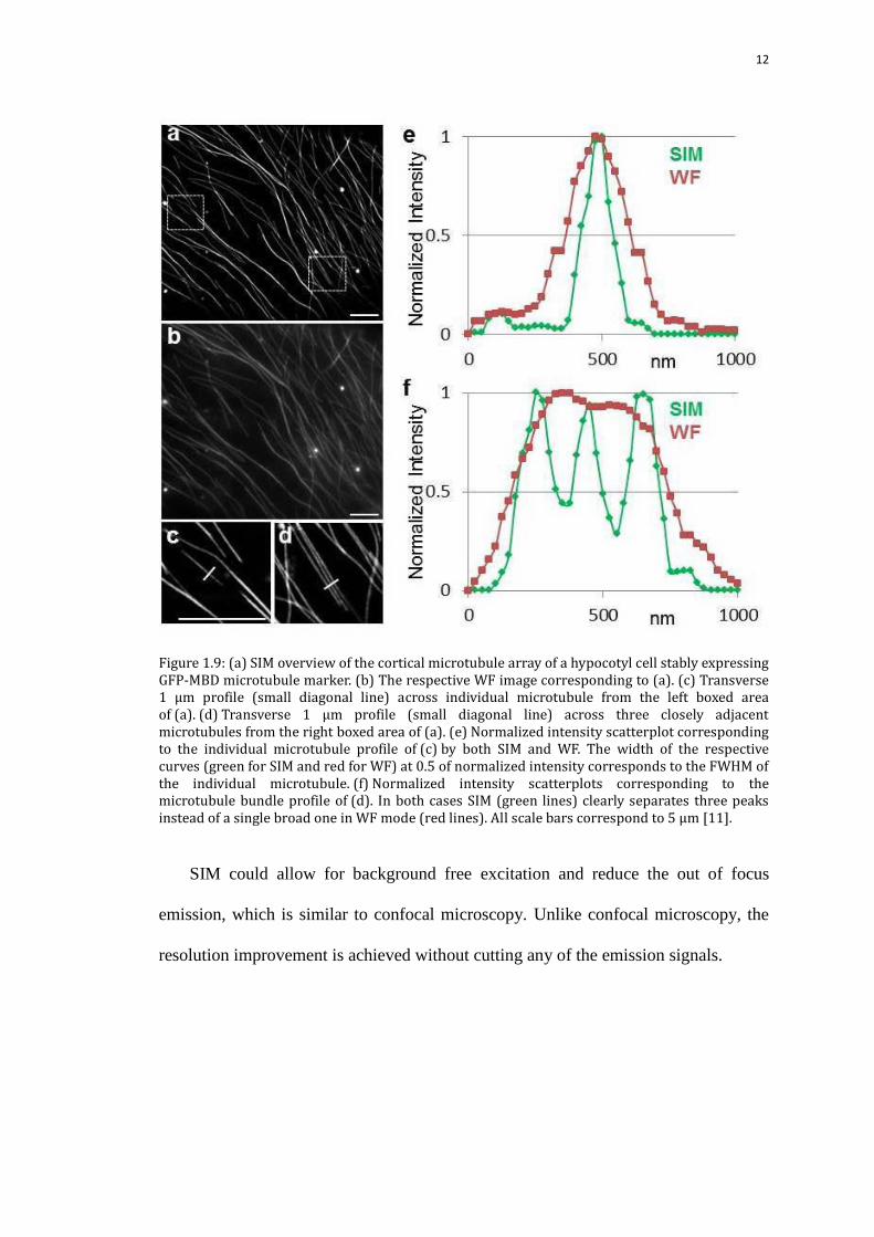
and an axial resolution reaching 120 nm, seen from Figure 1.9 [11].
12
Figure 1.9: (a) SIM overview of the cortical microtubule array of a hypocotyl cell stably expressing GFP-MBD microtubule marker. (b) The respective WF image corresponding to (a). (c) Transverse 1 μm profile (small diagonal line) across individual microtubule from the left boxed area of (a). (d) Transverse 1 μm profile (small diagonal line) across three closely adjacent microtubules from the right boxed area of (a). (e) Normalized intensity scatterplot corresponding to the individual microtubule profile of (c) by both SIM and WF. The width of the respective curves (green for SIM and red for WF) at 0.5 of normalized intensity corresponds to the FWHM of the individual microtubule. (f) Normalized intensity scatterplots corresponding to the microtubule bundle profile of (d). In both cases SIM (green lines) clearly separates three peaks instead of a single broad one in WF mode (red lines). All scale bars correspond to 5 μm [11].
SIM could allow for background free excitation and reduce the out of focus
emission, which is similar to confocal microscopy. Unlike confocal microscopy, the
resolution improvement is achieved without cutting any of the emission signals.

13
1.1.7 STED
STED microscopy improves the resolution by the selective deactivation of
fluorophores, minimizing the active emission area at the focal point [12]. When the
fluorophore is excited by the laser beam, the electron will be excited to the excitation
state and it will drop to the ground state and emit the photon through spontaneous
decay. No such photon will be emitted if an addition STED is introduced to pull the
electron to the ground state via stimulated emission. The STED microscopy utilizes
the STED to deplete the emission. The shape of the STED beam is engineered as
doughnut, and the minimum of the doughnut is overlapped with the excitation beam,
thus it could deplete the emission in the periphery and keep the signal in the central
part. In this way, the lateral and axial resolution could be improved using the 3D
doughnut.
The xy doughnut can be obtained through a vortex plate which is a twisted light
beam with an orbital angular momentum, causing a zero point at the center. The step
plate of which the central part has a pi phase difference with the outer part, provides a
doughnut in axis.
Ideally, the doughnut with a perfect zero overlapping with the excitation beam
could make the resolution infinitesimal with high STED power. The FWHM can be
described as
√
Where, I, Isat are the STED intensity and saturation intensity [13].
14
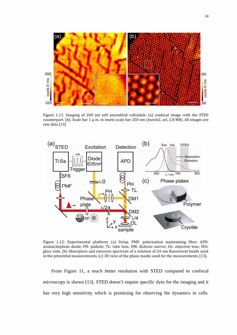
Figure 1.11: Imaging of 200 nm self assembled colloidals: (a) confocal image with the STED counterpart. (b). Scale bar 1 μ m, in insets scale bar 250 nm (movie2, avi, 2.8 MB). All images are raw data [13]
Figure 1.12: Experimental platform; (a) Setup. PMF: polarisation maintaining fibre; APD: avalanchephoto diode; PH: pinhole; TL: tube lens; DM: dichroic mirror; OL: objective lens; SF6: glass rods. (b) Absorption and emission spectrum of a solution of 24 nm fluorescent beads used in the presented measurements. (c) 3D view of the phase masks used for the measurements [13].
From Figure 11, a much better resolution with STED compared to confocal
microscopy is shown [13]. STED doesn‟t require specific dyes for the imaging and it
has very high sensitivity which is promising for observing the dynamics in cells.

15
While it remains a concern since the high power of STED may cause damage to the
sample, especially for the living cells.
1.1.8 STORM/PALM
Storm microscopy is based on high-accuracy localization of photo switchable
fluorophores. The storm imaging consists of a series of cycles. In each cycle, only a
small fraction of fluorophores is switched on, in other words, these fluorophores are
not overlapping, so their localizations could be obtained by 2D Gaussian fitting. The
localization accuracy is determined by the emitted photon numbers and usually in
nanometer scale. Repeating this for many cycles, each causing a stochastically
different subset of fluorophores to be switched on allows the positions of many
fluorophores to be determined and thus an overall image to be reconstructed [14].
The development of PALM [15] was quite prompted by the discovery of new
species and the engineering of mutants of fluorescent proteins displaying a
controllable photochromism, such as photo-activatable GFP. Similarly, STORM uses
paired cyanine dyes. Both techniques have been widely used and taken great
developments, in particular allowing multicolor imaging and the extension to three
dimensions, with the best current axial resolution of 10 nm in the third dimension
obtained using an interferometric approach [16].
These technique could enhance the resolution greatly, while the duty cycle is
really low, which limits its application in observing the dynamic in cell imaging.
16
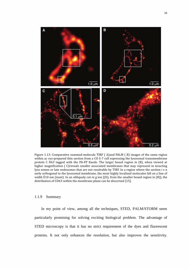
Figure 1.13: Comparative summed-molecule TIRF ( A)and PALM ( B) images of the same region within ac ryo-prepared thin section from a CO S-7 cell expressing the lysosomal transmembrane protein C D63 tagged with the PA-FP Kaede. The larger boxed region in (B), when viewed at higher magnification ( C)reveals smaller associated membranes that may represent in teracting lyso somes or late endosomes that are not resolvable by TIRF. In a region where the section i s n early orthogonal to the lysosomal membrane, the most highly localized molecules fall on a line of width È10 nm (inset). In an obliquely cut re g ion [(D), from the smaller boxed region in (B)], the distribution of CD63 within the membrane plane can be discerned [15].
1.1.9 Summary
In my point of view, among all the techniques, STED, PALM/STORM seem
particularly promising for solving exciting biological problem. The advantage of
STED microscopy is that it has no strict requirement of the dyes and fluorescent
proteins. It not only enhances the resolution, but also improves the sensitivity.

17
Furthermore, it enables direct observation of the dynamic at native environment in
cells. The disadvantage is that STED is technically complicated and the photon
toxicity remains a concern. On the other hand, PALM/ STORM are technically easier
to implement and a resolution of 20nm is possible to achieve, making it a very
powerful tool for studying the biological problem at single molecule level. However,
PALM / STORM require special photoactivatable or photoswitchable dyes [17], and
the low time duty will restrict the use of detecting the single molecules dynamically.
Over the last few decades, the super-resolution techniques have already had a
great impact on modern cell biology. These microscopy show great advance over
conventional microscopy, they also have their specific strengths and weaknesses as
discussed above. Among, I want to emphasis that as for photon statistics that create a
trade-off between spatial and temporal resolution [18], there still could be
improvement. And all these techniques would also depend on the rapid development
of more sensitive detectors, stable dyes and flexible lasers together with steady
electronic device. It is firmly believed that better techniques would continue showing
up. Another promising direction is the combinations of these super-resolution
techniques, such as the combination of 4pi with STED. With these techniques, many
new insights into cellular structure and function are to be expected in the near future.

18
1.2 Gene Expression
1.2.1 Mechanism: Transcription, RNA processing, Non-coding RNA maturation,
RNA export, Translation, Folding, Translocation, Protein transport
Gene is located on chromosomes and is the fundamental unit of heredity that
encodes genetic characteristics. Gene regulation controls the structure and function of
the cells, and is the basis for cellular differentiation, morphogenesis and the versatility
and adaptability of any organism [19]. Gene expression is the process by which the
information stored in a gene is used in the synthesis of a functional gene product,
typically proteins or functional RNAs. The process is tightly regulated so that a cell
could respond to its changing environment. Several steps featuring gene expression
may be modulated, including the transcription, RNA processing, Non-coding RNA
maturation, RNA export, Translation, Folding, Translocation, Protein transport.
Among them the two key steps in gene expression are transcription and translation.
Figure 1.13: an overview of the flow of information from DNA to protein in a eukaryote [20].

19
1.2.2 Transcription of Eukaryotic Protein-Coding Genes: Initiation, Promoter escape,
Elongation, Termination
Transcription is the first phase of gene expression, in which the encoded gene
information is copied into message RNA (mRNA) with the help of the RNA
polymerase and other transcription factors. The mRNA will function as the template
for the protein product during the translation process. The transcription consists of
Initiation, Promoter escape, Elongation and Termination.
1.2.3 RNA Polymerase II in transcription
In the thesis, I mainly focus on the role and properties of RNA polymerase II in
transcription. RNA polymerase is an enzyme that remarkably signatures transcription.
In the bacteria, RNA polymerase carries out the transcription of DNA into RNA in
which RNA polymerase initiates transcription at a promoter, synthesizes the RNA by
chain elongation, stops transcription at a terminator, and releases both the DNA
template and the completed mRNA molecule [21]. In eukaryotic cells, the process of
transcription is much more complicated, and there are three RNA polymerases:
polymerase I, II, and III among which RNA polymerase II plays the most important
role in synthesizing eukaryotic mRNA [22]. RNA polymerase II requires several
additional proteins and the general transcription factors to initiate transcription on a
purified DNA template, and still more proteins to initiate transcription on its
chromatin templates inside the cell.
20
1.2.3.1 RNA Polymerase II and initiation cofactors
First, with the transcription factor, the polymerase binds to the specific DNA
sequence called promoter to form a closed complex [23, 24]. The RNA polymerase
II–containing transcription initiation apparatus to promoters of protein-coding genes
is recruited by transcriptional activators. The assembled apparatus contains the
12-subunit RNA polymerase II core enzyme, the general transcription factors, and one
or more multisubunit complexes called coactivators or mediators. Second, assisted by
one or more general transcription factors, the polymerase unwinds the 14 nucleotides
of DNA to form open complex. Then polymerase finds the start site in the
transcription bubble, binds to an initiating NTP and an extending NTP complementary
to the sequence, and catalyzes bond formation to yield an initial RNA product.
In bacteria, RNA polymerase core enzyme consists of five subunits [25]: 2 α
subunits, 1 β subunit, 1 β' subunit, and 1 ω subunit and one general RNA transcription
factor: sigma. RNA polymerase core enzyme associate to sigma factor to form
holoenzyme and then binds to a promoter. In archaea and eukaryotes, RNA
polymerase contains additional subunits in addition to the five RNA polymerase
subunits in bacteria [26]. In archaea and eukaryotes, the functions performed by the
bacterial general transcription factor sigma are performed by multiple general
transcription factors that work together. In archaea, there are three general
transcription factors: TBP, TFB, and TFE. In eukaryotes, in RNA polymerase
II-dependent transcription, there are six general transcription
factors: TFIIA, TFIIB , TFIID , TFIIE , TFIIF, and TFIIH. Additional protein,
activators and repressors also take part in regulating the initiation.

21
1.2.3.2 RNA Polymerase II and elongation cofactors
One strand of DNA is used as a template for RNA synthesis [27]. As transcription
proceeds, RNA polymerase traverses the template strand and uses base pairing
complementary with the DNA template to create an RNA copy. The switch from
initiation to elongation involves phosphorylation of the RNA polymerase II CTD and
an exchange of cofactors associated with the polymerase. RNA polymerase II
molecules found in initiation complexes lack phosphate on their CTDs, while
elongating polymerase molecules contain heavily phosphorylated CTDs. The
Mediator complex is tightly associated with RNA polymerase II molecules that lack
phosphate on their CTDs in the holoenzyme. In contrast, the elongation complex and
various RNA processing factors become associated with RNA polymerase II
molecules with hyperphosphorylated CTDs. CTD phosphorylation must occur during
the transition from transcription initiation to elongation, because the phosphorylated
CTD has a role in recruiting the 1mRNA capping enzyme to the nascent transcript,
and mRNA capping occurs soon after promoter clearance. The exact mechanisms that
control the switch from initiation to elongation remain unknown.
1.2.4 Polymerase II Clustering
RNA polymerase II plays a significant role in gene expression, especially
transcription. Most related investigations are based on in vitro biochemical
experiments. The mechanism and properties of the RNA polymerase II in vivo is not
very clearly understood. In fact, a series of experiments regarding RNA polymerase
II in transcription argue on the existence of clustered Polymerase II [28, 29]. In higher
eukaryotes, messenger RNA (mRNA) synthesis is believed to involve foci of
22
clustered RNA polymerase II called transcription factories. However, clustered Pol II
has not yet been resolved in living cells, raising the debate about their existence in
vivo and what role, if any, they play in nuclear organization and regulation of gene
expression.
Different experiments have been performed to investigate the existence of the
accumulation of RNA polymerase II in living cells. Brief descriptions of some
classical experiments holding different views are listed below.
The first evidence suggesting that several transcription units cluster together dates
to the visualization of focal sites of transcription within human nuclei experiment [30].
The cells were permeabilized and the engaged polymerases were allowed to extedn
their transcripts in BrUTP (bromouridine triphosphate). And nascent BrRNA was
seen in a few discrete foci, basically the factories. From these fixed cells studies
emerged theories interpreting the Pol II clusters as static pre-assemblies termed
“transcription factories.” However, attempts to directly visualize Pol II clusters in
living cells had been initially unsuccessful, raising a debate over their existence in
vivo [31, 32].
Quantitative analysis [33] suggested that a typical transcription factory in the
nucleoplasm of a HeLa cell contains nearly 8 Polymerases, each involved a different
unit.
Two theoretical arguments suggest that components of the transcriptional
machinery are likely to cluster and so form factories [34]. First, many transcription
factors dimerize [35], and if they also bind to two sites on DNA that are a few kb
apart, they will inevitably loop the intervening DNA when they come together. As
GFP (green fluorescent protein)-tagging shows that many transcription factors remain
23
bound to DNA for only a second or so, such ties would be transient. Secondly, two
polymerases engaged several kb apart on one template are likely to come together
spontaneously in the crowded nucleus through what physicists call the
„depletion-attraction‟ [36, 37]. Loops formed in this way would last for as long as the
polymerases remain engaged, which can be for many hours in humans.
Based on the fact [32] that the largest catalytic subunit of the polymerase bears a
temperature-sensitive mutation in the CHO cell line, tsTM4 and the wild-type subunit
from human cells was tagged with GFP and expressed in tsTM4; this construct
complemented the defect at the restrictive temperature, enabling the mutant cells to
grow normally . This indicates that the tagged polymerase must be functional. As
these cells contain both endogenous and tagged polymerases, then they estimated their
relative contributions to the total polymerizing activity as follows: during elongation,
the COOH-terminal domain of the largest catalytic subunit becomes
hyperphosphorylated and reactive to the H5 antibody. As a result, this
hyperphosphorylated form is widely used as a marker for the active enzyme. Under
this growth conditions, immunoblotting indicates that most of the H5-reactive form in
the cell is the GFP-polymerase (GFP-pol) instead of the endogenous enzym. They use
these cells to analyze the mobility of the GFP-pol, concentrating on changes occurring
over the minutes required to complete a transcription cycle. Determining whether
GFP-pol diffuses as a core enzyme of nearly 500 kD or a larger complex of 1,000–
2,000 kD requires analysis over fractions of a second and the development of
fluorescent standards of appropriate size. However, no larger complexes involved in
repair have been detected. The kinetics are consistent with the result that roughly75%
of the GFP-polymerases are able to move rapidly, with the remainder being
transiently immobile (association t1/2 ≈ 20 min). No fraction immobilized in an
24
inactive preinitiation complex could be detected. They also used a conventional
biochemical approach of radiolabeling nascent transcripts with [3H]uridine to confirm
that the endogenous enzyme in wild-type cells completes a transcription cycle with
roughly similar kinetics. By estimating the length of a typical gene and the rate of
elongation, they calculate that a polymerase would be engaged for only one half to
five sixths of a transcription cycle; then, a typical expressed transcription unit would
actually be transcribed for only a minority of the time. In this paper, they didn‟t detect
the immobilized but in active polymerases, arguing against the existence of
polymerase clustering.
Sunney Xie‟s paper [38] argues against the existence of transcription factories in the
mammalian nucleaus. Combining reflected light-sheet illumination with
superresolution microscopy (PALM), they were able to image inside mammalian
nuclei at subdiffration limit resolution. With superior signal-to-background ratio as
well as molecular counting with single-copy accuracy, they probed the spatial
organization of transcription by RNA polymerase II (RNAP II) molecules and
quantified their global extent of clustering inside the mammalian nucleus. Knowing
that the photoblinking events of TMR tend to be clustered temporally, they developed
a reliable density-based clustering algorithm that pools multiple localizations based on
their proximity in space as well as in time. In this way, they could accurately assign
localizations to spatiotemporal clusters. Applying this technique to the one on one
labeled RNA polymerase II fixed RPB1 cells, they found that nearly 70% of the foci
consist of only 1 st-cluster, corresponding to only one RNAP II molecule, whereas the
fraction with 4 or more st-clusters is minimal (<10%).

25
Figure 1.14: Spatial organization of RNAP II molecules shows no significant clustering. (A) Distribution of SNAP-RPB1 molecules in a thin optical section of the nucleus of a fixed U2OS cell labeled with TMR. (Inset) Zoomed-in area where individual transcription foci are discernible; yellow crosses indicate the centroid position of the st-clusters identified. (Scale bar, 2 μm; Inset, 500 nm.) (B) Distribution of the number of st-clusters in transcription foci indicates that at least 70% of the foci consist of only one RNAP II molecule (n = 4,465). (C) Distribution of spatial NND for transcription foci shows that the majority of the RNAP II molecules do not associate with each other within the reported diameter of transcription factories (40–130 nm). Dotted line indicates the mean [38].
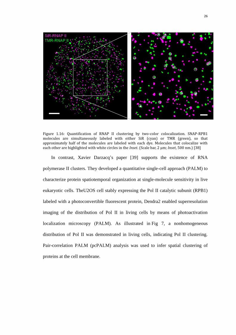
In addition, they quantified the polymerase II clustering using two color
colocalization. They labeled the SNAP-RPB1 molecules simultaneously with SiR and
TMR dyes approximately equally under the fine-tuned labeling conditions. If there is
clustering of two or more RNAP II molecules, at least half of them will be revealed as
colocalized signals of the two dyes. Two-color superresolution imaging and
colocalization analysis detected 17.9 ± 1.0% (n = 8,929 in six cells) of the molecules
that colocalize with each other, thus yielding a maximum of 35.8 ± 2.0% of the
clusters with more than one RNAP II molecule, supporting the conclusion that most
of the foci contains only 1 polymerase II.
26
Figure 1.16: Quantification of RNAP II clustering by two-color colocalization. SNAP-RPB1 molecules are simultaneously labeled with either SiR (cyan) or TMR (green), so that approximately half of the molecules are labeled with each dye. Molecules that colocalize with each other are highlighted with white circles in the Inset. (Scale bar, 2 μm; Inset, 500 nm.) [38]
In contrast, Xavier Darzacq‟s paper [39] supports the existence of RNA
polymerase II clusters. They developed a quantitative single-cell approach (PALM) to
characterize protein spatiotemporal organization at single-molecule sensitivity in live
eukaryotic cells. TheU2OS cell stably expressing the Pol II catalytic subunit (RPB1)
labeled with a photoconvertible fluorescent protein, Dendra2 enabled superresolution
imaging of the distribution of Pol II in living cells by means of photoactivation
localization microscopy (PALM). As illustrated in Fig 7, a nonhomogeneous
distribution of Pol II was demonstrated in living cells, indicating Pol II clustering.
Pair-correlation PALM (pcPALM) analysis was used to infer spatial clustering of
proteins at the cell membrane.

27
Figure 1.15: Fig. 1Live-cell superresolution imaging reveals spatial Pol II clustering. (A)
Preconverted (Dendra2-RPB1 green emission) fluorescence image shows Pol II primarily
localized in nucleus [compare (A) and (B)]. (B) Two-dimensional superresolution reconstruction
reveals nonhomogeneous distribution of detected Pol II (red). Nuclear contour (white outline) is
approximated from preconverted fluorescence in (A). (C) A pair-correlation analysis was
implemented as previously described (12) to quantitatively analyze the spatial distribution.
Represented is the pair-correlation function computed from the spatial coordinates of the raw
PALM detections (black), fitted to a general function (orange) that accounts for contributing
factors from the protein clusters and single-molecule stochastic effects as detailed in
supplementary text and fig. S3. The corrected spatial correlation function for the protein (green)
is decoupled from the fluorophore stochastic contributions (blue). The corrected protein
correlation function shows statistically significant clustering, above the theoreticalg(r) = 1 (gray
dashes) with a fit parameter of rprotein ~ 220 (± 17) nm, distinct from the single-molecule
stochastic fit parameter of rstoch ~ 45 (± 1) nm. Errors (in parentheses) represent standard
error of the fitted value [39].
TcPALM, namely combining time-correlated detection counting and PALM as
28
time-correlated PALM, revealed that the time series representing the rate of detection
of Dendra2Pol II fluorescence are not uniformly distributed and these temporal
clustering events are more evident in the cumulative count of detections, where they
appear as large steps.
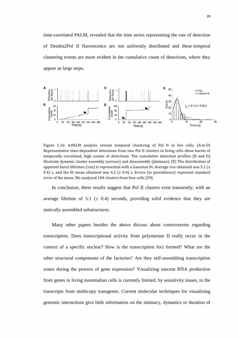
Figure 1.16: tcPALM analysis reveals temporal clustering of Pol II in live cells. (A to D)
Representative time-dependent detections from two Pol II clusters in living cells show bursts of
temporally correlated, high counts of detections. The cumulative detection profiles (B and D)
illustrate dynamic cluster assembly (arrows) and disassembly (plateaus). (E) The distribution of
apparent burst lifetimes (τon) is represented with a Gaussian fit. Average τon obtained was 5.1 (±
0.4) s, and the fit mean obtained was 4.2 (± 0.4) s. Errors (in parentheses) represent standard
error of the mean. We analyzed 104 clusters from four cells [39].
In conclusion, these results suggest that Pol II clusters exist transiently, with an
average lifetime of 5.1 (± 0.4) seconds, providing solid evidence that they are
statically assembled substructures.
Many other papers besides the above discuss about controversies regarding
transcription. Does transcriptional activity from polymerase II really occur in the
context of a specific nuclear? How is the transcription foci formed? What are the
other structural components of the factories? Are they self-assembling transcription
zones during the process of gene expression? Visualizing nascent RNA production
from genes in living mammalian cells is currently limited, by sensitivity issues, to the
transcripts from multicopy transgenes. Current molecular techniques for visualizing
genomic interactions give little information on the intimacy, dynamics or duration of

29
interactions. Development of techniques to better visualize chromosomal interactions
over time would greatly enhance our understanding of these processes.
In this thesis, I demonstrate a real-time tracking, ultra-sensitive optical nanoscopy
system that enables single-molecule detection in addressable sub-diffraction volumes,
at high background concentrations within crowded intracellular environments.
Basically, the STED beam could deplete the emission and we engineer the STED
beam like a 3D doughnut and overlap the beam with the excitation beam, so that the
STED beam would deplete the background in the periphery and keep the central
signal. By spatial on off control of the fluorescence, the signal to noise ratio is
enhanced and sensitivity is improved. This idea is initially brought up by my advisor
Dr. Alexandros Pertsinidis. To investigate the properties of polymerase II as well as
other transcriptional units, a tracking system is built to restrain the units of interest at
the minimum of the STED beam. The proof of principle experiments in vivo
proposed by Dr. Alexandros Pertsinidis show that the nanoscopy could greatly
increase the sensitivity and enable single molecule detection at hundreds of
nanomolar, which is close to the endogenous environment of living cells. To image
Pol II dynamics in relation to transcription from a defined promoter, a “mini-gene”
system is designed by Dr. Alexandros Pertsinidis and my labmate Jieru Li to
visualize the position of the genomic locus in the nucleus and track production of
nascent RNA simultaneously in real-time. The clustered polymerase II is observed and
the properties are quantified.
30
Chapter Two
Numerical simulation of single molecule
detection using STED

31
2. Numerical Simulation of single molecule detection using STED
Prior to building the STED nanoscopy, I conducted some numerical simulation in
order to have a better understanding of the mechanism and choose the optimal and
practical optical setup. Basically there are 4 parts in the simulation: excitation, STED,
Emission and Detection.
The 642nm red excitation and the 780nm STED beam are used for the simulation.
The xy doughnut is from a vortex plate with a helical ramp which leads to the
continuous phase change from 0 to 2π in the azimuthal direction. The light will cancel
each other at the center thus leading to a zero intensity there. For the z doughnut, the
step plate with a π phase shift in the central circle would give a z doughnut by
adjusting the relative size of the inner circle of step plate.
2.1 Numerical Simulation Theory
As we know, not all integrals can be computed. However, we could always
estimate values of definite integrals by regarding the integral as an area problem and
using simply shapes to approximate the area under the curve. In my simulation, I did
the numerical calculations using the Midpoint Rule [40].
To estimate the integral,
∫
We divide the interval [a, b] into n subintervals of equal width,

32
Let us denote each of the intervals as follows,
[ , ], [ , ],……, [ , ], where = a and = b
Next let be the midpoint of the interval. We can easily find the area for each could
be approximated by the area of a collection of rectangles whose heights are
determined by
∫
∑
2.2 Excitation beam
According to the theory by Wolf and Richards [41], I numerically investigated the
vectorial electric field near the focus point.
Figure 2.1: The meridional plane of a ray. The axis Ox is in the direction of the electric vector e𝑜 in the object space. From the paper of Wolf and Richards [41]
The equations describing the x, y, z components of the electric field are derived by
Wolf and Richards.

33
After numerically calculating the values of e , e , e , we further computed the
intensity distribution in the focal volume using the relationship that
e e +e e e e
With the calculated intensity distribution, I quantified the lateral and axial full width
at half maximum (FWHM) using Gaussian fitting.
The FWHMs were investigated on the conditions with different numerical
aperture values ranging from 0.3 to 1.35. Next, I studied how FWHM would vary
with NA with all the other parameters fixed.
In lateral, I got the fitting result as
. ( = 642nm, n =1.33)
e e e e
√
No surprisingly, and behaved the same way on NA as
circularly polarized light was used for the simulation. As a matter of fact, the intensity
distribution in xy plane is isotropic.

34
Figure 2.2: FWHM(nm) vs NA in x direction
Figure 2.3: FWHM(nm) vs NA in y direction
Figure 2.4: FWHM(nm) vs NA in z direction

35
2.3 Vortex doughnut
The vortex plate shown in Figure 2.5 [42] introduces continuous phase change
from 0 to 2Mπ in the azimuthal direction. Here M is a positive integer and the so
called charge. Mathematically, an additional term shall be multiplied by the
integrand for calculating the electric field for excitation beam.
Figure 2.5: Vortex plate [42]
Without any calculation, I derived analytically that at the very center (0, 0, 0), the
intensity is perfect zero. If I focus on the integrations on , we can get the following
conclusions as well (M is the charge of the vortex):
a. M = 1,
For left-handed circularly polarized light, I (0, 0, 0) = (0, 0, 0);
For right-handed circularly polarized light, I (0, 0, 0) = (0, 0, a), (a ! =0)
b. M >= 2,
For both left-handed and right-handed circularly polarized light,
I (0, 0, 0) = (0, 0, 0)
The numerical approximation provided us with the intensity distribution of the xy
doughnut sometimes called vortex doughnut. Figure 2.6 and 2.7 illustrates the nice

36
looking xy doughnut in focal plane and in xz plane respectively. The zero in the
center is vital since no depletion is desired in the center.
Figure 2.6: The intensity of the donut on the focal plane, the wavelength of the beam is 780nm
Figure 2.7: The intensity of the donut on xz plane (y=0), the wavelength of the beam is 780nm
2.4 Z doughnut
2.4.1 Central intensity with different phase modulation
To realize 3D super resolution imaging, I utilized z depletion pattern with step
plate z-beam depletion [43]. The extra Pi phase shift in the center could result in
37
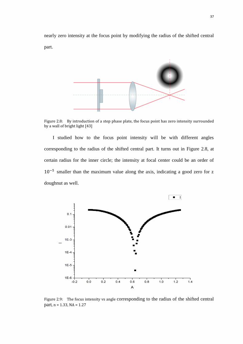
nearly zero intensity at the focus point by modifying the radius of the shifted central
part.
Figure 2.8: By introduction of a step phase plate, the focus point has zero intensity surrounded by a wall of bright light [43]
I studied how to the focus point intensity will be with different angles
corresponding to the radius of the shifted central part. It turns out in Figure 2.8, at
certain radius for the inner circle; the intensity at focal center could be an order of
smaller than the maximum value along the axis, indicating a good zero for z
doughnut as well.
Figure 2.9: The focus intensity vs angle corresponding to the radius of the shifted central
part, n = 1.33, NA = 1.27
38
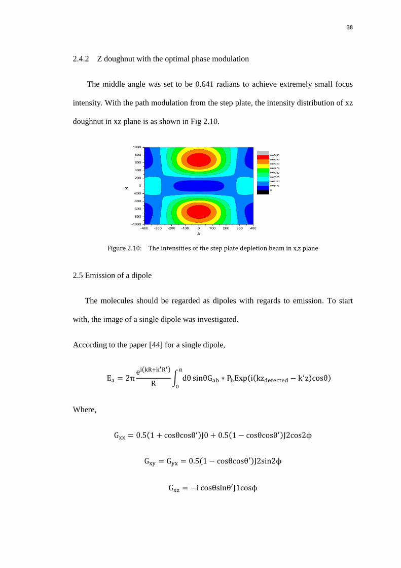
2.4.2 Z doughnut with the optimal phase modulation
The middle angle was set to be 0.641 radians to achieve extremely small focus
intensity. With the path modulation from the step plate, the intensity distribution of xz
doughnut in xz plane is as shown in Fig 2.10.
Figure 2.10: The intensities of the step plate depletion beam in x,z plane
2.5 Emission of a dipole
The molecules should be regarded as dipoles with regards to emission. To start
with, the image of a single dipole was investigated.
According to the paper [44] for a single dipole,
e ( )
∫
Where,

39
J0, J1, J2 denote Bessel function of the first kind with argument k
√
Upon these equations, I got the intensity following roughly Gaussian distribution
in the focal plane by numerical simulation. Simulation of dipoles with different
orientations showed different distributions. What‟s more, the center coordinates of
detected image will vary with the initial object positions in the focal space.
Figure 2.10: The image of a dipole at x=y=z=0, theta = Pi

40
Figure 2.11: The image of a dipole at x=50, y=100, z=150, theta = Pi
2.6 Resolution with different combinations of xy and z doughnut
A combination of xy and z step plate doughnut beam will not only deplete the
emissions on z axis but also on the xy plane. By adjusting the ratio of xy and z
doughnut power, I could achieve a isotropic 3D doughnut in the space.
I_sted = M*I_donut + N*I_stedz.
Different values set for M and N in table 2.1 lead to spherical spots of different
sizes. Typically, it is commonsensible that higher Power gives rise to sharper PSF.
M(100*Is) N(100*Is) FWHMxy(nm) FWHMz (nm)
1.7 0.07 120.09 120.80
7.2 0.75 60.16 60.24
30 3.8 30.12 30.16
Table 2.1: Choose different input powers of the donut beam and step plate beam to get nearly spherical spots with radius of 60nm, 30nm, 15nm
41
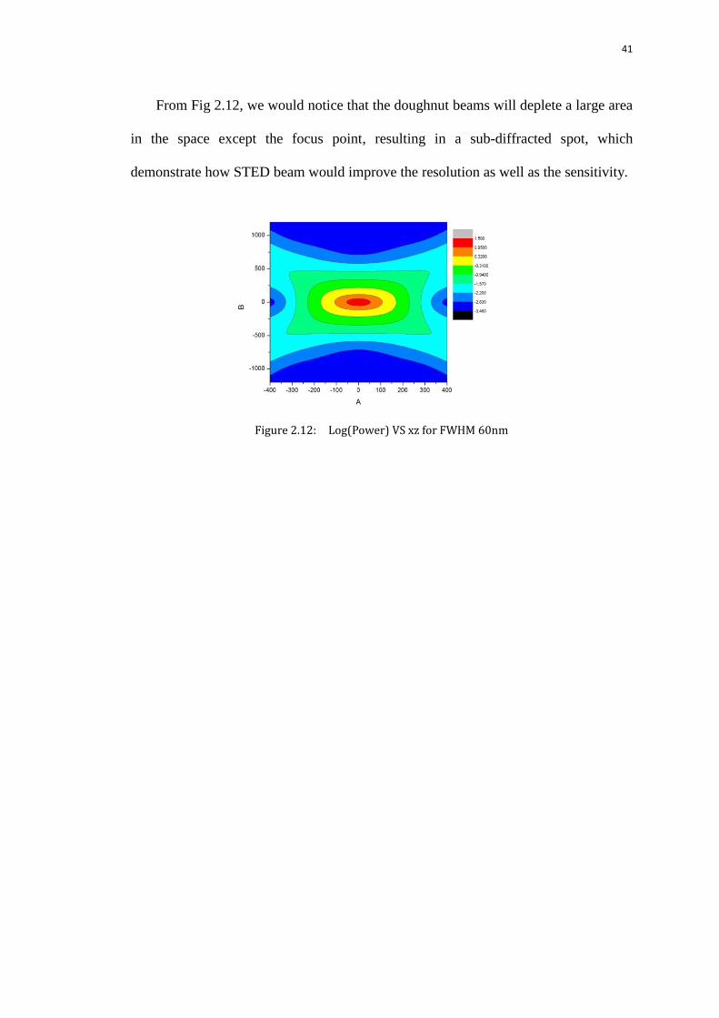
From Fig 2.12, we would notice that the doughnut beams will deplete a large area
in the space except the focus point, resulting in a sub-diffracted spot, which
demonstrate how STED beam would improve the resolution as well as the sensitivity.
Figure 2.12: Log(Power) VS xz for FWHM 60nm

42
Chapter Three
Experimental Setup
43
3. Experimental Setup
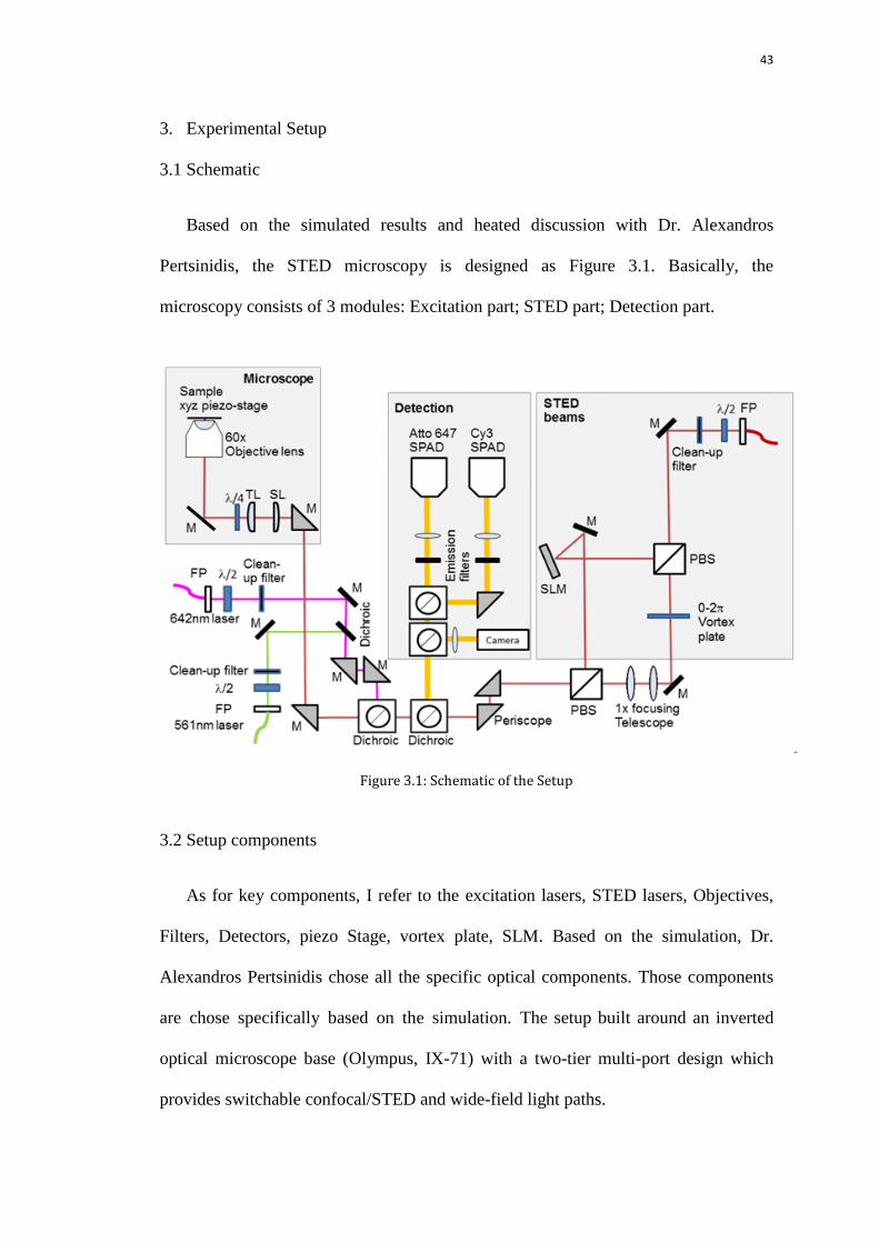
3.1 Schematic
Based on the simulated results and heated discussion with Dr. Alexandros
Pertsinidis, the STED microscopy is designed as Figure 3.1. Basically, the
microscopy consists of 3 modules: Excitation part; STED part; Detection part.
Figure 3.1: Schematic of the Setup
3.2 Setup components
As for key components, I refer to the excitation lasers, STED lasers, Objectives,
Filters, Detectors, piezo Stage, vortex plate, SLM. Based on the simulation, Dr.
Alexandros Pertsinidis chose all the specific optical components. Those components
are chose specifically based on the simulation. The setup built around an inverted
optical microscope base (Olympus, IX-71) with a two-tier multi-port design which
provides switchable confocal/STED and wide-field light paths.
44
For the excitation part, there are two pulsed laser diodes operating at 490nm and
640nm (Pico-Quant, LDH-P-C-485B and LDH-P-C-640B, controlled by Sepia 828-S 2
channel driver) and a 561nm CW solid-state laser (Cobolt, Jive 500).
Beam from Titanium-sapphire oscillator passed through an Electro-optic
Modulator (Conoptics, model 350-80) that enabled fast modulation of laser intensity,
and then was coupled into the fiber. In Figure 3.1, the STED beam was split into two
beams by the PBS: one went through the vortex plate which is a helical ramp providing
a smooth angular increase from 0 to 2π, resulting in a doughnut like beam in xy plane;
the other beam got reflected by the spatial light modulator (Hamamatsu, LCOS-SLM
X10468-02) which imposed programmed spatially varying modulation. In our case, the
SLM functioned as a step plate, adding additional π phase shift in the inner circle with
adjustable size on the beam. The SLM modulated the beam to a z doughnut beam. After
going through a couple of optics including the 60x silicon oil immersed objective lens,
the two doughnut beams merged and overlapped with the excitation beams on the
sample. Some 1x focusing telescopes would be used for adjusting the collimations of
all the beams to overlap the beams. The sample sit on a direct drive, high-dynamics 3D
nanopositioning stage equipped with capacitive sensors (Physik Instrumente,
P-561.3DD), interfaced to a digital controller (Physik Instrumente E-710 or E-712).
The emitted fluorescent light propagated back to the detectors. A 50:50 PBS could be
inserted to divide the signals into two parts: one arrives at the APDs suited for
scanning confocal/STED images; the other half signal would be collect by the
quad-view CCD camera. The quad-view images are used for real time tracking.
45
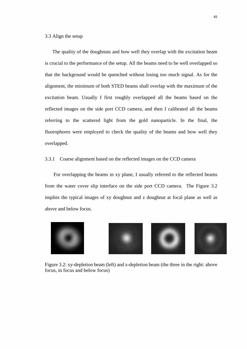
3.3 Align the setup
The quality of the doughnuts and how well they overlap with the excitation beam
is crucial to the performance of the setup. All the beams need to be well overlapped so
that the background would be quenched without losing too much signal. As for the
alignment, the minimum of both STED beams shall overlap with the maximum of the
excitation beam. Usually I first roughly overlapped all the beams based on the
reflected images on the side port CCD camera, and then I calibrated all the beams
referring to the scattered light from the gold nanoparticle. In the final, the
fluorophores were employed to check the quality of the beams and how well they
overlapped.
3.3.1 Coarse alignment based on the reflected images on the CCD camera
For overlapping the beams in xy plane, I usually referred to the reflected beams
from the water cover slip interface on the side port CCD camera. The Figure 3.2
implies the typical images of xy doughnut and z doughnut at focal plane as well as
above and below focus.
Figure 3.2: xy-depletion beam (left) and z-depletion beam (the three in the right: above
focus, in focus and below focus)
46
3.3.2 Calibrate the beams using gold nanoparticle (PMT used)
Based on the simulated results, I have a sense of the shapes of the beams. It is
indispensable to calibrate the exact shape of all the beams for this specific setup.
Furthermore, the calibration provides a point of reference for overlapping the beams.
3.3.2.1 xz scanning
The way to calibrate the setup is to scan over the gold nanoparticles and collect the
scattered light by gold nanoparticles. The gold nanoparticles stick to the glass cover slip
nonspecifically with glue the fraction index of which is close to the immersion oil was
prepared and mounted on the piezo stage. Once one particle was found, I roughly
centered it on the focus by checking the reflected images on the side port CCD camera.
Next the wave generator in E710\E712 scans a pre-defined trajectory over the particle
with stationary excitation and STED beams. The actual trajectory was recorded using
the stage capacitive sensors. A typical 4um×4um in xz or xy plane, 8second scan
consisted of 80 lines and 8000 points were sampled to obtain the actual trajectory of the
stage (100 points/line)
The scattered back propagated to the PMT. PMT converted the photon into
electronic signal and amplified the signal. Later the signal sampled at a frequency of
200 KHz, together with the trigger signal from E710\E712 for marking the first point of
each trajectory lines, was sent to shielded connector block with BNC (BNC2110,
National Instrument). Labview software was written to send commands to E710\E712
and dynamically acquire the signals from BNC 2110. The matlab script embedded in
the Labview constructed the 4by4um cofocal images. In matlab2010, the signals after
low pass filtration and smoothing over every 40 sample points were first binned to
100ms and synchronized with the scanning positions. Then I interpolated the irregular

47
sample trajectory with the corresponding photon signals to a 200 by 200 mesh grid. At
last, I binned the pixel to make the pixel size 40 nm.
In Figure 3.3, the xz profiles of the red excitation, vortex doughnut and z doughnut
were calibrated. I optimized the beams, especially for the z doughnut and then
overlapped them in xz plane. Different step phase modulations were tried to obtain a
symmetrical z doughnut with a close to zero central part, referring to these calibrations.
Figure 3.3: xz profiles of a. Excitation; b. Vortex doughnut; c. Z doughnut
3.3.2.2 xy scanning
Similarly, I calibrated the xy profiles of the red excitation, vortex doughnut and z
doughnut. The calibration process was exactly the same as that for xz profile calibration
except that the scanning pattern applied to xy plane. The xy profiles of the exaction,
vortex doughtnut and z doughnut beam in Figure 3.4 look tight and symmetrical, more
importantly the beams are well overlapped.
Figure 3.4: xy profiles of a. Excitation; b. Vortex doughnut; c. Z doughnut

48
3.3.3 Quarter wave plate adjustment
We learnt from the simulation that the orientation of the quarter wave plate is
crucial to the quality of the vortex doughnut. Left-handed circularly polarized beam is
requisition of perfect zero for xy doughnut. Referring to the reflected image on the
side port CCD camera, the angle of the quarter wave plate was optimized.
3.3.4 Optimal collar position for Silicon oil and regular oil objective
Most microscope objectives are designed to work with a cover glass that has a
standard thickness of 0.17 millimeters and a refractive index of 1.515, which is
satisfactory when the objective numerical aperture is less than 0.4. However, when
using high numerical aperture dry objectives, cover glass thickness variations of only
a few micrometers result in dramatic image degradation due to aberration, which
grows worse with increasing cover glass thickness. To compensate for this error, the
objectives are equipped with a correction collar to allow adjustment of the central lens
group position to coincide with fluctuations in cover glass thickness. The objectives
are composed of a series of optical components. The collar position corresponds to the
different position of those optical components. Although coverslips with a thickness
of 0.17 millimeters are used in our situation, the high numerical value of 1.3 requires
optimization of the collar positions to ensure the quality of the beams. The scale of
objective ranges from 1.3 to 1.9. Comparing the calibrated profiles of excitation,
vortex doughnut and z doughnut at each collar positions with a rotating step size of
0.1, I Figured out the optimal collar position for the silicon oil objective is 0.15 at 25
degree, and 0.16 at 37 degree. The optimization was characterized by tightest focus
spots, less spherical aberration and minimal center of the doughnuts.
49
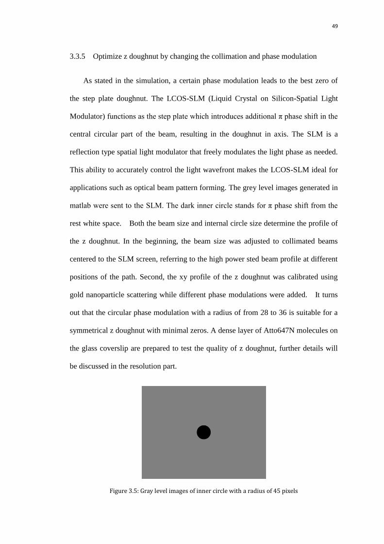
3.3.5 Optimize z doughnut by changing the collimation and phase modulation
As stated in the simulation, a certain phase modulation leads to the best zero of
the step plate doughnut. The LCOS-SLM (Liquid Crystal on Silicon-Spatial Light
Modulator) functions as the step plate which introduces additional π phase shift in the
central circular part of the beam, resulting in the doughnut in axis. The SLM is a
reflection type spatial light modulator that freely modulates the light phase as needed.
This ability to accurately control the light wavefront makes the LCOS-SLM ideal for
applications such as optical beam pattern forming. The grey level images generated in
matlab were sent to the SLM. The dark inner circle stands for π phase shift from the
rest white space. Both the beam size and internal circle size determine the profile of
the z doughnut. In the beginning, the beam size was adjusted to collimated beams
centered to the SLM screen, referring to the high power sted beam profile at different
positions of the path. Second, the xy profile of the z doughnut was calibrated using
gold nanoparticle scattering while different phase modulations were added. It turns
out that the circular phase modulation with a radius of from 28 to 36 is suitable for a
symmetrical z doughnut with minimal zeros. A dense layer of Atto647N molecules on
the glass coverslip are prepared to test the quality of z doughnut, further details will
be discussed in the resolution part.
Figure 3.5: Gray level images of inner circle with a radius of 45 pixels
50
3.3.6 Overlap all the beams
Generally, the vortex doughnut and z doughnut are overlapped and in some cases
the collimation of xy doughnut could be modified to overlap the two doughnuts by
adjusting the relative distance of the telescope. Usually aligning the beams is a matter
of overlapping the excitation beams with the STED beams. The focus could be
modified by changing the collimation of the beams. The telescopes for each excitation
beams, together with the fiber ports, provide ranges of collimation. The xz profiles
were measured by gold nanoparticle calibration. All the beams could be aligned to
focus with 100nm.
3.4 Resolution vs power
One remarkable feature of STED microscopy is the enhancement of its resolution
[45]. With the optimized and overlapped beams, I demonstrated the improvement of the
resolution with STED beams.
3.4.1 Immobile molecules sample preparation
To verify the lateral resolution, I prepared a sample of Atto647N binding on the
glass coverslips. Glass coverslips and slides were passivated with 4-arm
Poly-ethylene-glycol (PEG) [465]. The 15bp Cy3-Atto647N duplex was immobilized
on the PEG coverslip surface through biotin-streptavidin interactions. An
Atto647N-labeled oligo was then diluted at 100-600nM in imaging buffer (75mM
HEPES-KOH pH 7.5, 55mM Potassium Glutamate, 1.8% w/v Glucose, 1mM Ascorbic
Acid, 1mM Methyl Viologen, glucose oxidase and catalase enzymes and 500µM
random10nt oligo), flowed in and the sample was sealed with tape. The buffer could
scavenge the oxygen in the solution, which would lower the possibility of photon
beaching.

51
An extremely dense layer of Atto647N was prepared in xz plane to quantify the
axial resolution. Similarly, 20uL 250nM 15bp Cy3-Atto647N duplex was injected in
the channel between the PEG glass coverslip and slide via the drained holes in the slide.
The channel was then rinsed with 20uL 1x PBS after over 30 minutes incubation. Again,
the oxygen scavenger was put into the channel to reduce photon bleaching.
3.4.2 Later resolution vs STED power
A 2µm×2µm region was first scanned in 8 seconds with 66µW 642nm excitation
only, followed by a second scanning with 66µW 642nm plus STED 780nm beams. The
single photon sensitive τ-SPAD detectors have very high sensitivity and good timing
resolution of 350 picoseconds (FWHM), making a great candidate for STED
microscopy. The NIM signal, together with the markers for E712\E710, was first saved
as binary file in Picoharp. The offline analysis was performed in matlab2010. The
arrival times of each photon were extracted from the binary file. The photon signals
were synchronized with the 8000 sampling positions by the markers at the first point of
each scanning trajectory lines sent by E710\E712. Similar way as described in the
calibration part was used to construct the 2D images. By comparison of the 2D cofocal
images with and without STED, we apparently visualized the enhancement of lateral
resolution with xy STED doughnut. The cofocal image was a typical diffraction limited
spot with a FWHM of 250nm, while with 250mw 780nm vortex doughnut STED beam,
the sharp image was characterized with a FWHM of 93nm.
52
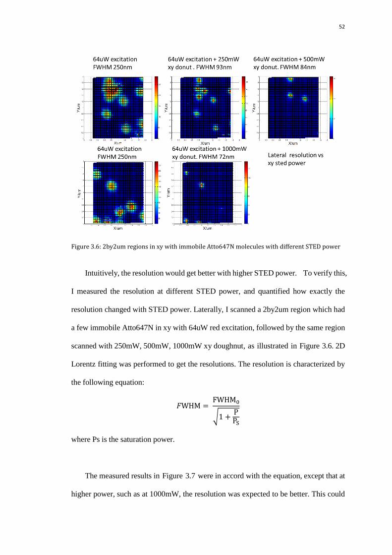
Figure 3.6: 2by2um regions in xy with immobile Atto647N molecules with different STED power
Intuitively, the resolution would get better with higher STED power. To verify this,
I measured the resolution at different STED power, and quantified how exactly the
resolution changed with STED power. Laterally, I scanned a 2by2um region which had
a few immobile Atto647N in xy with 64uW red excitation, followed by the same region
scanned with 250mW, 500mW, 1000mW xy doughnut, as illustrated in Figure 3.6. 2D
Lorentz fitting was performed to get the resolutions. The resolution is characterized by
the following equation:
√
where Ps is the saturation power.
The measured results in Figure 3.7 were in accord with the equation, except that at
higher power, such as at 1000mW, the resolution was expected to be better. This could
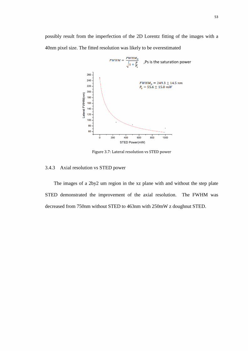
53
possibly result from the imperfection of the 2D Lorentz fitting of the images with a
40nm pixel size. The fitted resolution was likely to be overestimated
Figure 3.7: Lateral resolution vs STED power
3.4.3 Axial resolution vs STED power
The images of a 2by2 um region in the xz plane with and without the step plate
STED demonstrated the improvement of the axial resolution. The FWHM was
decreased from 750nm without STED to 463nm with 250mW z doughnut STED.
,Ps is the saturation power
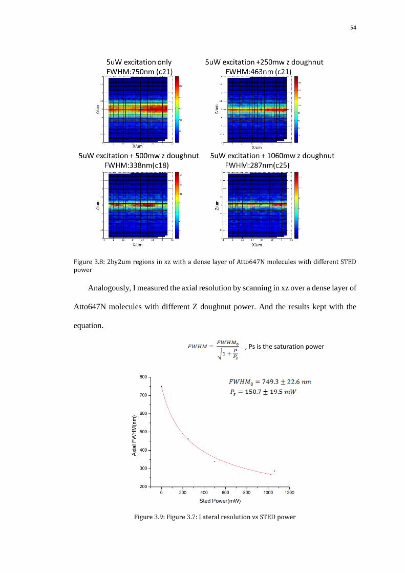
54
Figure 3.8: 2by2um regions in xz with a dense layer of Atto647N molecules with different STED power
Analogously, I measured the axial resolution by scanning in xz over a dense layer of
Atto647N molecules with different Z doughnut power. And the results kept with the
equation.
Figure 3.9: Figure 3.7: Lateral resolution vs STED power
, Ps is the saturation power
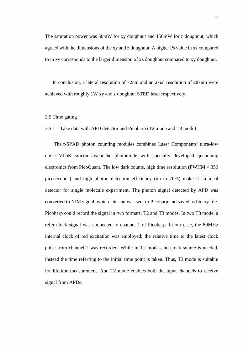
55
The saturation power was 50mW for xy doughnut and 150mW for z doughnut, which
agreed with the dimensions of the xy and z doughnut. A higher Ps value in xz compared
to in xy corresponds to the larger dimension of xz doughnut compared to xy doughnut.
In conclusion, a lateral resolution of 72nm and an axial resolution of 287nm were
achieved with roughly 1W xy and z doughnut STED laser respectively.
3.5 Time gating
3.5.1 Take data with APD detector and Picoharp (T2 mode and T3 mode)
The τ-SPAD photon counting modules combines Laser Components' ultra-low
noise VLoK silicon avalanche photodiode with specially developed quenching
electronics from PicoQuant. The low dark counts, high time resolution (FWHM < 350
picoseconds) and high photon detection efficiency (up to 70%) make it an ideal
detector for single molecule experiment. The photon signal detected by APD was
converted to NIM signal, which later on was sent to Picoharp and saved as binary file.
Picoharp could record the signal in two formats: T2 and T3 modes. In two T3 mode, a
refer clock signal was connected to channel 1 of Picoharp. In our case, the 80MHz
internal clock of red excitation was employed; the relative time to the latest clock
pulse from channel 2 was recorded. While in T2 modes, no clock source is needed,
instead the time referring to the initial time point is taken. Thus, T3 mode is suitable
for lifetime measurement. And T2 mode enables both the input channels to receive
signal from APDs.
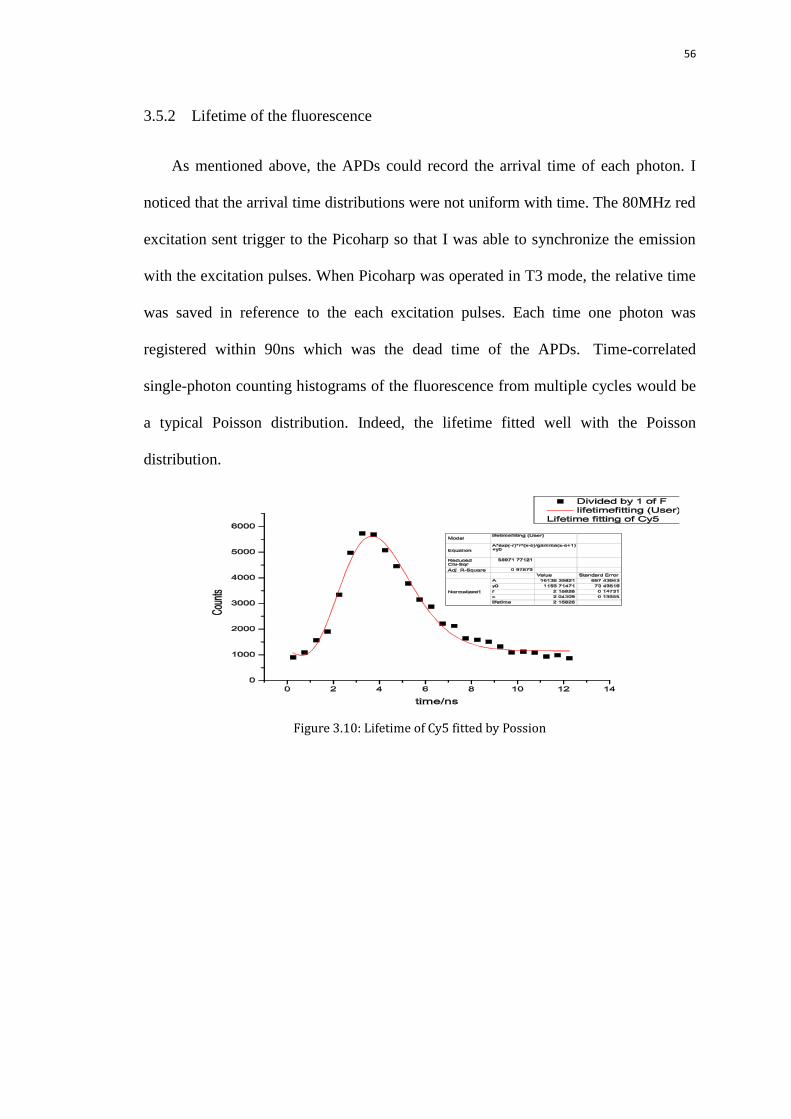
56
3.5.2 Lifetime of the fluorescence
As mentioned above, the APDs could record the arrival time of each photon. I
noticed that the arrival time distributions were not uniform with time. The 80MHz red
excitation sent trigger to the Picoharp so that I was able to synchronize the emission
with the excitation pulses. When Picoharp was operated in T3 mode, the relative time
was saved in reference to the each excitation pulses. Each time one photon was
registered within 90ns which was the dead time of the APDs. Time-correlated
single-photon counting histograms of the fluorescence from multiple cycles would be
a typical Poisson distribution. Indeed, the lifetime fitted well with the Poisson
distribution.
Figure 3.10: Lifetime of Cy5 fitted by Possion
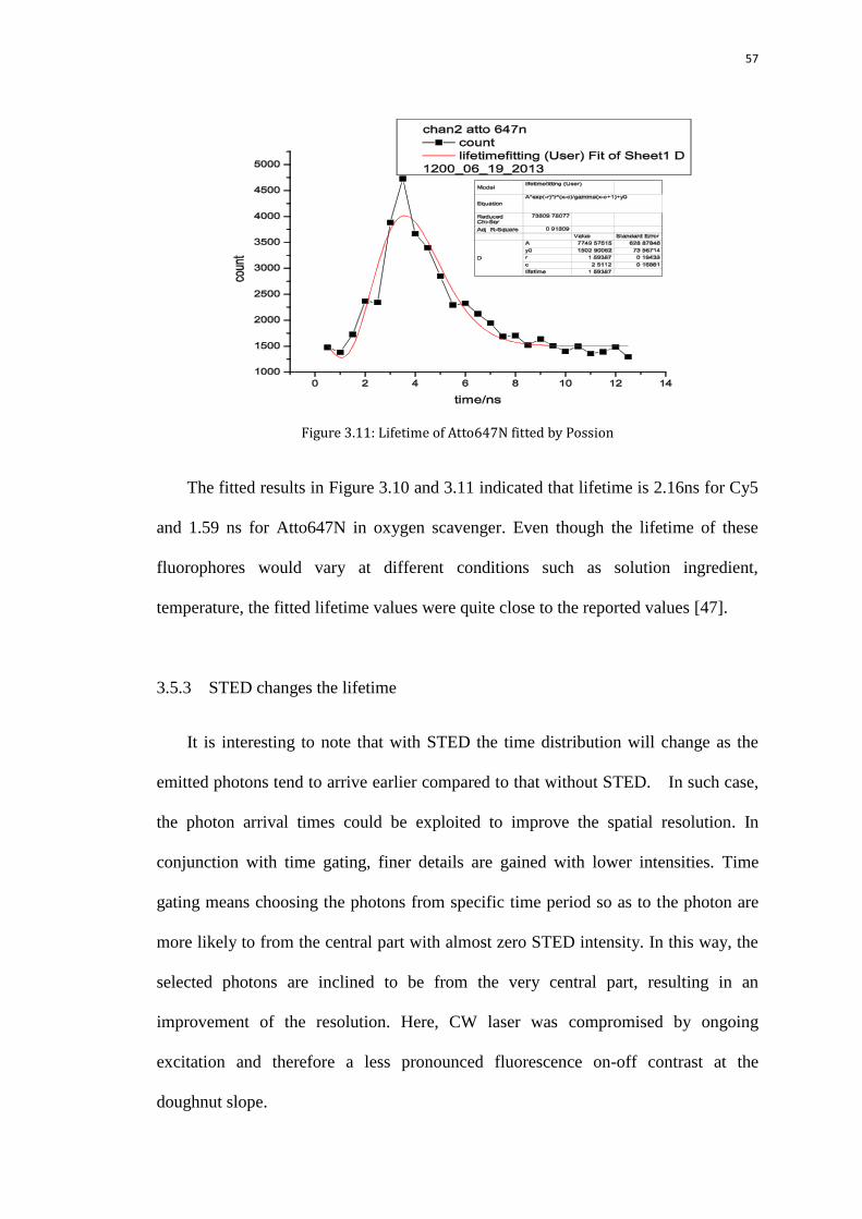
57
Figure 3.11: Lifetime of Atto647N fitted by Possion
The fitted results in Figure 3.10 and 3.11 indicated that lifetime is 2.16ns for Cy5
and 1.59 ns for Atto647N in oxygen scavenger. Even though the lifetime of these
fluorophores would vary at different conditions such as solution ingredient,
temperature, the fitted lifetime values were quite close to the reported values [47].
3.5.3 STED changes the lifetime
It is interesting to note that with STED the time distribution will change as the
emitted photons tend to arrive earlier compared to that without STED. In such case,
the photon arrival times could be exploited to improve the spatial resolution. In
conjunction with time gating, finer details are gained with lower intensities. Time
gating means choosing the photons from specific time period so as to the photon are
more likely to from the central part with almost zero STED intensity. In this way, the
selected photons are inclined to be from the very central part, resulting in an
improvement of the resolution. Here, CW laser was compromised by ongoing
excitation and therefore a less pronounced fluorescence on-off contrast at the
doughnut slope.
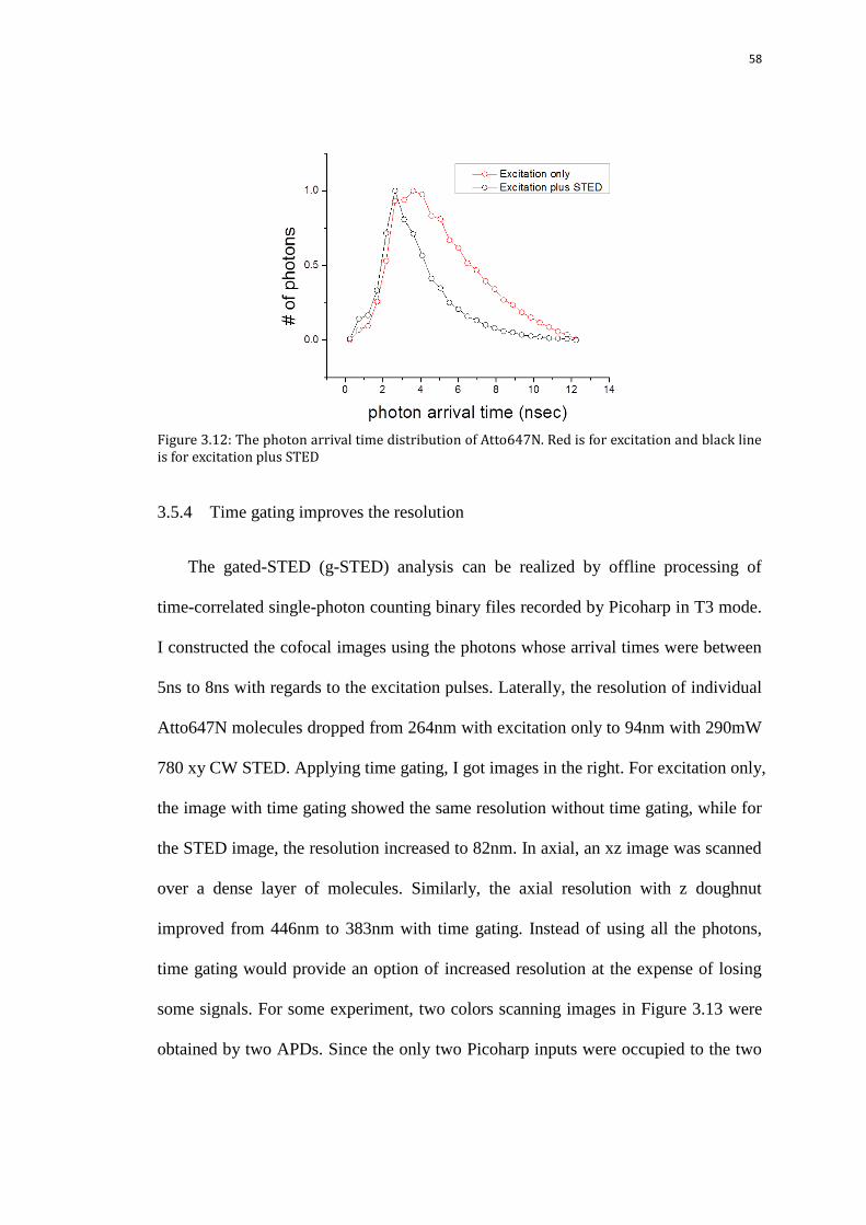
58
Figure 3.12: The photon arrival time distribution of Atto647N. Red is for excitation and black line is for excitation plus STED
3.5.4 Time gating improves the resolution
The gated-STED (g-STED) analysis can be realized by offline processing of
time-correlated single-photon counting binary files recorded by Picoharp in T3 mode.
I constructed the cofocal images using the photons whose arrival times were between
5ns to 8ns with regards to the excitation pulses. Laterally, the resolution of individual
Atto647N molecules dropped from 264nm with excitation only to 94nm with 290mW
780 xy CW STED. Applying time gating, I got images in the right. For excitation only,
the image with time gating showed the same resolution without time gating, while for
the STED image, the resolution increased to 82nm. In axial, an xz image was scanned
over a dense layer of molecules. Similarly, the axial resolution with z doughnut
improved from 446nm to 383nm with time gating. Instead of using all the photons,
time gating would provide an option of increased resolution at the expense of losing
some signals. For some experiment, two colors scanning images in Figure 3.13 were
obtained by two APDs. Since the only two Picoharp inputs were occupied to the two

59
APDs, the Picoharp would only function in T2 mode. In such case, time gating could
not be applied [48].
Figure 3.13 Confocal images of Atto647N in xz plane without (left) and with(right) time gating : a. 642nm Excitation only; b. 642nm Excitation and 418mW 780nm z doughnut STED
3.6 CW laser vs pulsed mode laser
3.6.1 Pulsed mode properties
The previously demonstrated results were with CW STED lasers. Historically,
Stephen Hell first built STED with pulsed lasers. Pulsed lasers would deplete the
fluorescence more efficiently. However, pulsed lasers are more complicated to handle
with. What‟s more, the temporal alignment between excitation pulses and STED
pulses is required. In other words, the STED pulses need to be synchronized with the
excitation pulses with an adjustable time delay. Only the two pulses arrived at the
sample at the same time, we could get the most efficient depletion. Furthermore, the
width of the STED pulses should be optimized to overlay the excitation pulses without
getting stretched too much. To achieve the same resolution, less power is required for
Pulsed STED laser.

60
3.6.2 Optimize the phase to achieve the highest depletion
In practice, the Mira OPO enables the Ti:Sapphire to switch from CW mode to
pulsed mode. Two 6-inch glass rods stretched the pulse width to ~300fs to avoid
unwanted non-linear effects and damage to the fiber. The 80MHz trigger signals were
sent out from the STED laser controller. The phase was adjusted by the Analog
Voltage Control Phase Shifter 60-80MHz 180° Full Band before it was sent to
trigger the excitation controller (Sepia II).The Phase Shifter has a 0–15 V control
voltage range, corresponding to a 180 degree phase shift range.
A 300nM Atto647N molecules solution with oxygen scavenger was prepared to
Figure out the optimal voltage to achieve best depletion for the pulsed STED laser. I
measured the depletion with a starting voltage of 0V and a 0.1 V step increase to 15V.
3.6.3 Compare the two modes
When the laser was in pulsed mode, the maximum power is roughly quarter of that
in CW mode. The maximum power in pulsed mode was approximately 80mW,
corresponding to 290mW in CW mode. In spite of which mode the laser was in, the
depletion efficiency tested was quite close. Considering this situation, I operated the
STED laser in CW to avoid the process of synchronizing the pulsed STED with
excitation pulses.

61
Chapter Four
STED improves SNR and enable single
molecule detection in vivo
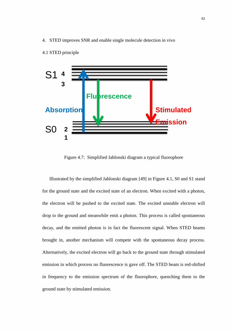
62
4. STED improves SNR and enable single molecule detection in vivo
4.1 STED principle
Figure 4.7: Simplified Jablonski diagram a typical fluorophore
Illustrated by the simplified Jablonski diagram [49] in Figure 4.1, S0 and S1 stand
for the ground state and the excited state of an electron. When excited with a photon,
the electron will be pushed to the excited state. The excited unstable electron will
drop to the ground and meanwhile emit a photon. This process is called spontaneous
decay, and the emitted photon is in fact the fluorescent signal. When STED beams
brought in, another mechanism will compete with the spontaneous decay process.
Alternatively, the excited electron will go back to the ground state through stimulated
emission in which process no fluorescence is gave off. The STED beam is red-shifted
in frequency to the emission spectrum of the fluorophore, quenching them to the
ground state by stimulated emission.
S0
S1
1
2
3
4
Fluorescence
Absorption Stimulated
Emission
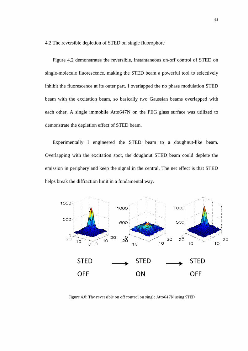
63
4.2 The reversible depletion of STED on single fluorophore
Figure 4.2 demonstrates the reversible, instantaneous on-off control of STED on
single-molecule fluorescence, making the STED beam a powerful tool to selectively
inhibit the fluorescence at its outer part. I overlapped the no phase modulation STED
beam with the excitation beam, so basically two Gaussian beams overlapped with
each other. A single immobile Atto647N on the PEG glass surface was utilized to
demonstrate the depletion effect of STED beam.
Experimentally I engineered the STED beam to a doughnut-like beam.
Overlapping with the excitation spot, the doughnut STED beam could deplete the
emission in periphery and keep the signal in the central. The net effect is that STED
helps break the diffraction limit in a fundamental way.
Figure 4.8: The reversible on off control on single Atto647N using STED
STED
ON
STED
OFF
STED
OFF

64
4.3 The general Background properties
For realizing single molecule detections in living cells which usually feature with
high background and very noisy, I need focus on reducing the background
fluctuations. Before that, it is necessary to study the properties of the background and
noise. Two main types of background fluctuations are assumed to dominate for
different systems: open system and closed system [50, 51,52]. Dr. Alexandros
Pertsinidis figured out the theory for the background properties. It turns out the
background noise is super Possion rather than Possion as people assumed. Dr.
Alexandros Pertsinidis explained the behaviors of noise in closed system and open
system as follows.
4.3.1 Closed system
In a closed system which does not allow the molecules transfer in or out of the
system, the number of the molecules in the system is constant; hence shot noise due to
the stochastic nature of fluorescence emission would dominate. In this case, the
intensity follows Poisson distribution. Assuming the intensity is given by
Where n is the total number of the molecules in the system, is the brightness of
single molecule.
Following the Poisson distribution, the variance is noted as

65
Thus we could derive that the SNR is
√ √
Based on this equation, we can only be able to achieve single molecule detection
when is high enough.
4.3.2 Open system
Accordingly, in an open system, such as the freely diffusing molecules in the
detection volume, the number of the molecules n would fluctuate and is Poisson
distributed.
√
The intensity fluctuate will be
In this case,
√
Irrespective of molecular brightness, single-molecule detection becomes
impossible since SNR will be always less than 1 for certain concentrations (n>>1).
4.4 The STED depletion in the Atto647N solution at different concentration
4.4.1 Background and noise from the solution and surface
Under low brightness conditions (0.5 < ε < 3), often used in fluorescence
correlation spectroscopy, small deviations from Poisson (characteristic of number

66
fluctuations) were seen in the tails of the photon-counting (intensity) histogram at
~1-50nM molecules in solution. It was further intuitively proposed that the relative
effect of number fluctuations diminishes at high concentrations, with the largest
deviations from Poisson expected at increasing ε and decreasing n. However, the
molecular concentration and brightness regimes where (Poisson) shot noise and
(super-Poisson) number fluctuations respectively dominate, and how these relate to
conditions relevant to single-molecule detection (ε >> 1), have not been fully
characterized. I measured the background level and noise for Atto647N-streptavidin
solutions at concentrations ranging from 15nM to 1µM. Strikingly, under illumination
conditions used for real-time single-molecule detection we observe noise that exceeds
several-fold the Poisson limit, while the Fano factor (variance/mean) increases
proportionally with excitation power (i.e. molecular brightness ε), independently of
concentration. These results strongly suggest that single-molecule detection at up to
1µM solution concentrations is largely limited by super- Poisson noise due to number
fluctuations.
4.4.2 Background and noise with different excitation power
To validate the noise at high concentration is super-Poisson, the background and
noise were investigated with different excitation power. As we expected, when the
excitation power exceeded a level which ensured ε >> 1, the SNR should be
independent of the excitation power, which was observed from the 15nM and 500nM
Atto647N solution. 5.53uW, 15.2uW and 66uW excitation power were illumined in

67
the Atto647N solution. The SNR stayed nearly the same level as the power increased,
indicating the noise is super Poisson.
Figure 4.9: SNR with different excitatio power at Atto647N solution of 15nM (black) and 500nM
(red)
4.4.3 Background and noise with and without STED of the Atto647N solution at
different concentration
The engineered 3D doughnuts will reduce the molecular brightness and thus
background level by a factor inversely proportional to the depletion saturation. The
backgrounds in the Atto647N solution at 15, 50, 150, 500 and 1200nM were
compared with and without STED. The Atto647n streptavidin solution in the
oxygen scavenger buffer was injected into the channel between the glass coverslip
and glass slide. The channel was previously blocked by 10% BSA for 10 minutes.
0 10 20 30 40 50 60 70
10
20
30
40
50
60
70
SN
R
Excitation power (uW)
15nM
500nM

68
Also 10uM streptavidin was mixed in the solution to reduce nonspecific binding of
Atto647N to the surface.
The STED was periodically turned on-off. Illustrated in Figure 22, fluorescence
intensity trace from 150nM Atto647N-streptavidin solution was less noisy and the
level got lower with 900mw xy doughnut beam on. Photon-counts were binned
every 10 milliseconds.
STED On
0 200 400 600 800 1000
500
1000
1500
2000
2500
3000
3500
4000
4500
ba
ckg
rou
nd
(co
un
ts/0
.01
s)
time(0.1s)
Figure 10.4: the background with periodically on off 900mW xy doughnut in 150nM Atto647N
solution
According to the quantified background level and noise reduction, the noise
reduction was proportional to the background level reduction. Application of STED
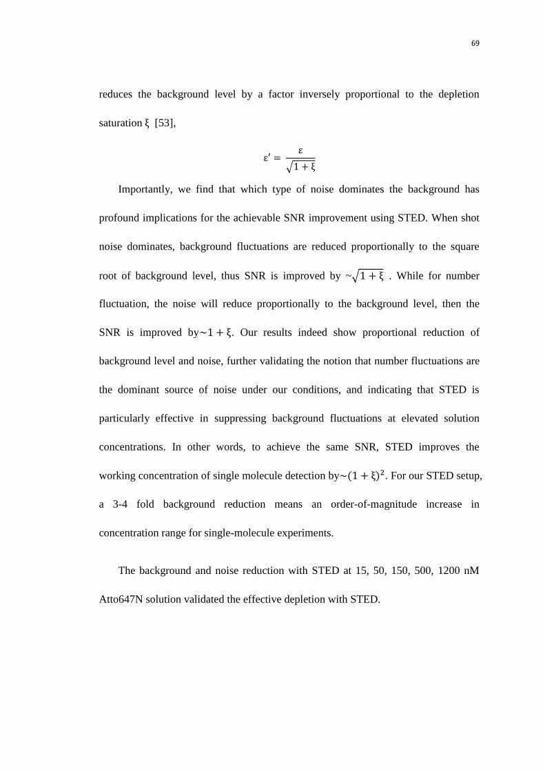
69
reduces the background level by a factor inversely proportional to the depletion
saturation [53],
√
Importantly, we find that which type of noise dominates the background has
profound implications for the achievable SNR improvement using STED. When shot
noise dominates, background fluctuations are reduced proportionally to the square
root of background level, thus SNR is improved by ~√ . While for number
fluctuation, the noise will reduce proportionally to the background level, then the
SNR is improved by . Our results indeed show proportional reduction of
background level and noise, further validating the notion that number fluctuations are
the dominant source of noise under our conditions, and indicating that STED is
particularly effective in suppressing background fluctuations at elevated solution
concentrations. In other words, to achieve the same SNR, STED improves the
working concentration of single molecule detection by . For our STED setup,
a 3-4 fold background reduction means an order-of-magnitude increase in
concentration range for single-molecule experiments.
The background and noise reduction with STED at 15, 50, 150, 500, 1200 nM
Atto647N solution validated the effective depletion with STED.
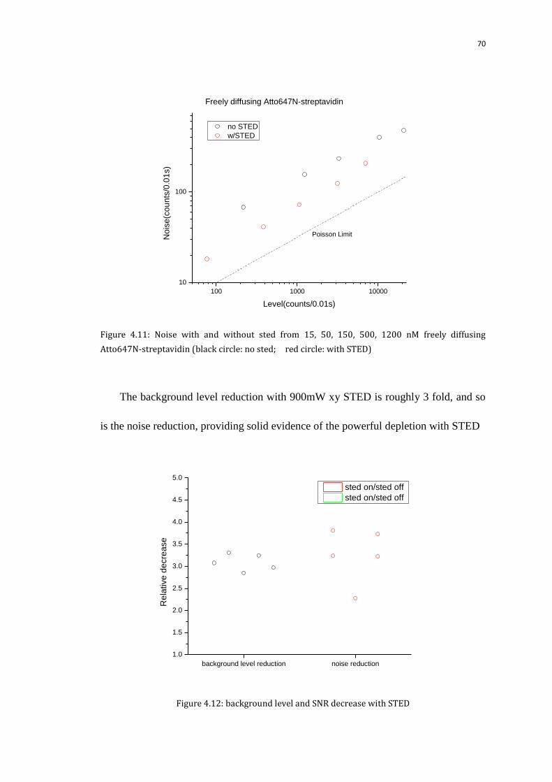
70
100 1000 10000
10
100
no STED
w/STED
No
ise
(co
un
ts/0
.01
s)
Level(counts/0.01s)
Freely diffusing Atto647N-streptavidin
Poisson Limit
Figure 4.11: Noise with and without sted from 15, 50, 150, 500, 1200 nM freely diffusing
Atto647N-streptavidin (black circle: no sted; red circle: with STED)
The background level reduction with 900mW xy STED is roughly 3 fold, and so
is the noise reduction, providing solid evidence of the powerful depletion with STED
background level reduction noise reduction
1.0
1.5
2.0
2.5
3.0
3.5
4.0
4.5
5.0
Re
lative
de
cre
ase
sted on/sted off
sted on/sted off
Figure 4.12: background level and SNR decrease with STED

71
As a matter of fact, we cared more about whether this applied to the in vivo
situation. While how STED would work in living cells remained unclear. Thus, I
measured the background and noise reduction with STED inside Rpb9 SiR Hela cells.
The cells were fully stained to retain the high background and noise level. 5.5uW red
excitation and 400mW xy doughnut and 700mW z doughnut were used. The
background and noise inside RPB9 cells behaved the way as in vitro that the noise
level reduction is proportional to background level reduction, proving STED is
potential for live cell imaging.
10 100 1000 10000
1
10
100
1000 red only
sted on
No
ise
(co
un
ts/0
.01
s)
Level (counts/0.01s)
Figure 4.13: Background level and noise with and without STED in RPB9 cells
3~4 fold reduction for the background level as well as for the noise was
demonstrated, verifying STED would also work inside the cells as efficiently as in
vitro. The data analysis was conducted by Dr. Alexandros Pertsinidis and me.
Alexandros drawed figure 4.11 and 4.12.
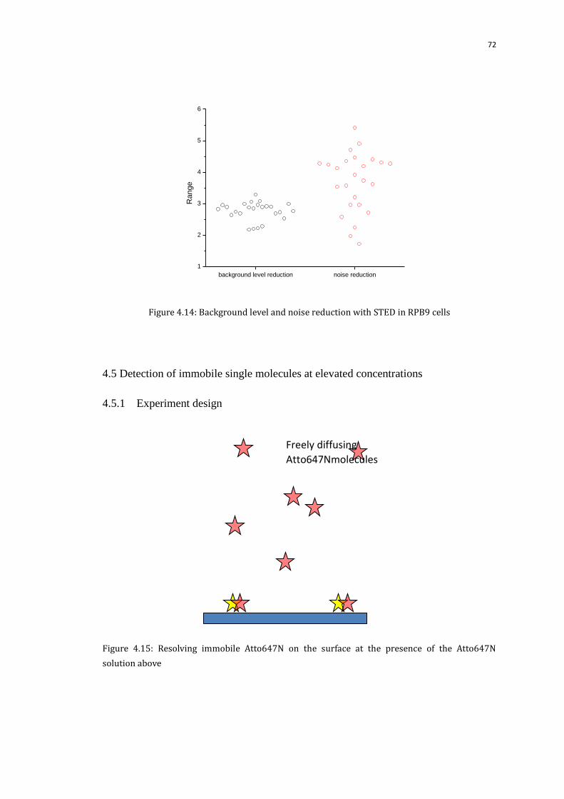
72
background level reduction noise reduction
1
2
3
4
5
6
Ra
ng
e
Figure 4.14: Background level and noise reduction with STED in RPB9 cells
4.5 Detection of immobile single molecules at elevated concentrations
4.5.1 Experiment design
Figure 4.15: Resolving immobile Atto647N on the surface at the presence of the Atto647N
solution above
Freely diffusing
Atto647Nmolecules

73
To demonstrate that STED enables single molecule detection at high
concentrations, I aimed to resolve the immobile molecules on the surface with the
background from the solution above. 15nt Cy3-Atto647N duplexes (IDT,
Cy3-biotin target oligo and 5‟Atto647N-AGATGAGGAAGAGAGT-3‟, HPLC
purified) were bound to the PEG surface. 100nM, 300Nm, 600nM Atto647N solution
with oxygen scavenger was put into the channels respectively to act as the
background. Alexandros designed the experiment.
4.5.2 Cy3-Atto647N duplex preparation
The two complementary oligos, Plac-70...-48 FWD 5‟Cy3 biotin and
Plac-48…-70 REV 5‟ Atto647N, were annealed to get the Cy3-Atto647N duplex.
1.5uL FWD Primer and 1.5uL REV Primer were diluted by 47uL 0.22um filtered
TE50 buffer. The mixture was incubated in the PCR machine with the Cyler settings:
the initial temperature was 95 degree, followed by a decrease of 10 degree every
minute till 25 degree, and then the temperature was set to 4 degree for 10 minutes.
The colocalization of Cy3 and Atto647N via FRET [54] indicated that the duplex
usually have a colocalization rate of over 40%, which is suitable for the following
surface experiment.
4.5.3 Map the yellow channel and red channel
The Cy3 was used to identify the corresponding Atto647N.Coordinate mapping
transformations were calibrated using cofocal images of stable 15bp Cy3-Atto647N
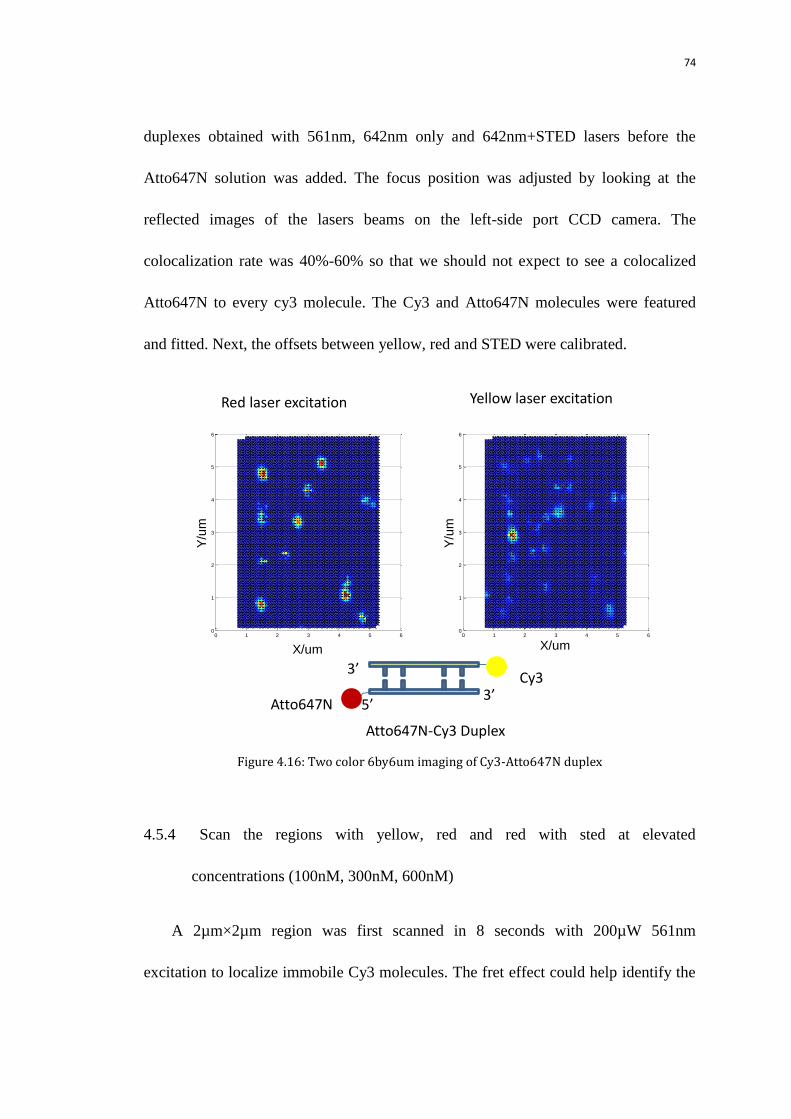
74
duplexes obtained with 561nm, 642nm only and 642nm+STED lasers before the
Atto647N solution was added. The focus position was adjusted by looking at the
reflected images of the lasers beams on the left-side port CCD camera. The
colocalization rate was 40%-60% so that we should not expect to see a colocalized
Atto647N to every cy3 molecule. The Cy3 and Atto647N molecules were featured
and fitted. Next, the offsets between yellow, red and STED were calibrated.
Figure 4.16: Two color 6by6um imaging of Cy3-Atto647N duplex
4.5.4 Scan the regions with yellow, red and red with sted at elevated
concentrations (100nM, 300nM, 600nM)
A 2µm×2µm region was first scanned in 8 seconds with 200µW 561nm
excitation to localize immobile Cy3 molecules. The fret effect could help identify the
0 1 2 3 4 5 60
1
2
3
4
5
6
X/um
Y/u
m
0 1 2 3 4 5 60
1
2
3
4
5
6
X/um
Y/u
m
Red laser excitation Yellow laser excitation
5’
Cy3
Atto647N
3’
3’
Atto647N-Cy3 Duplex

75
colocalized Atto647N. The same region was then scanned two more times, once with
66µW 642nm excitation only, followed by 66µW 642nm plus 200mW STEDxy and
600mW STEDz 780nm beams.
4.5.5 Construct and compare the images
At the presence of the 300nM Atto647N solution, we could hardly visualize the
Atto647N molecules from the red only cofocal image; while with STED beams on,
we could clearly observe there were 3 molecules showing up. The same results
applied to the 100nM, 600nM Atto647N solutions. With 600nM Atto647N solution
above, we could visualize nothing from red excitation cofocal image. In contrast, the
molecules could be resolved with STED on and colocalized with the Cy3s as well as
the Atto647Ns through Fret effect, which directly demonstrated the powerful effect of
STED.
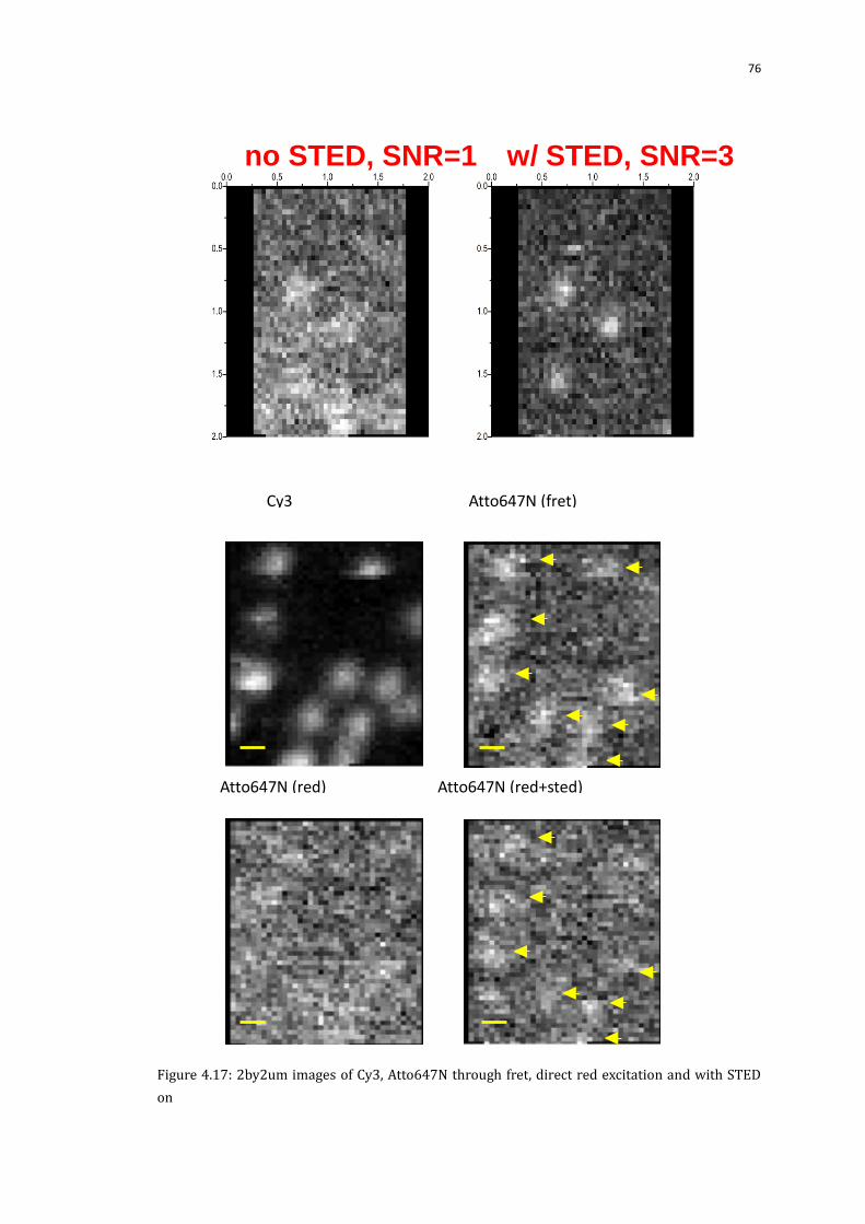
76
Figure 4.17: 2by2um images of Cy3, Atto647N through fret, direct red excitation and with STED
on
no STED, SNR=1 w/ STED, SNR=3
Cy3 Atto647N (fret)
Atto647N (red) Atto647N (red+sted)

77
4.5.6 Quantify the SNR with and without STED (The distribution of the signal from
the Cy3 colocalized regions and random regions)
Reconstructed 2D images were analyzed by calculating the total Atto647N
photon counts within a certain radius r from the Cy3 position and comparing with
total photon counts from equal size regions where there was no Cy3 detected. The
parameter r was set to 180 nm for excitation only and 100 nm for excitation and
STED respectively, which were roughly the sizes of the excitation beam without and
with STED. The peak of the signal from the cy3 colocalized regions was more
separate with that from random regions with STED beam (Background) since the
STED would reduce the background and the noise.
Figure 4.18: the total counts distribution from the cy3 colocalized regions (Molecules) and
random regions (Background) without and with STED
135000 150000 165000 180000 1950000
5
10
15
20
25
30
35
40
# r
egio
ns
Total counts
Background
Molecules
12000 13500 15000 16500 18000 195000
10
20
30
40
50
60
70
80
# r
egio
ns
Total counts
Background
Molecules
No STED With STED
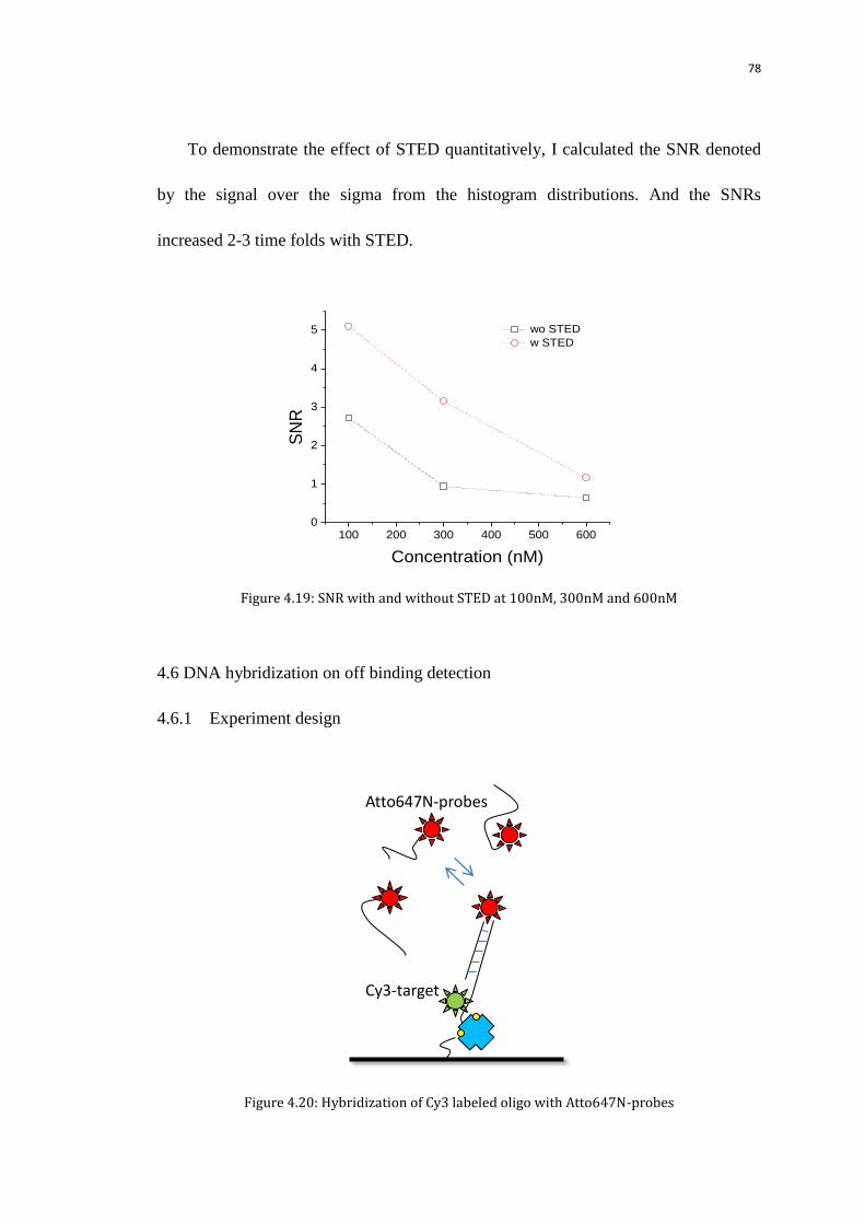
78
To demonstrate the effect of STED quantitatively, I calculated the SNR denoted
by the signal over the sigma from the histogram distributions. And the SNRs
increased 2-3 time folds with STED.
Figure 4.19: SNR with and without STED at 100nM, 300nM and 600nM
4.6 DNA hybridization on off binding detection
4.6.1 Experiment design
Figure 4.20: Hybridization of Cy3 labeled oligo with Atto647N-probes
100 200 300 400 500 6000
1
2
3
4
5
SN
R
Concentration (nM)
wo STED
w STED
Atto647N-probes
Cy3-target
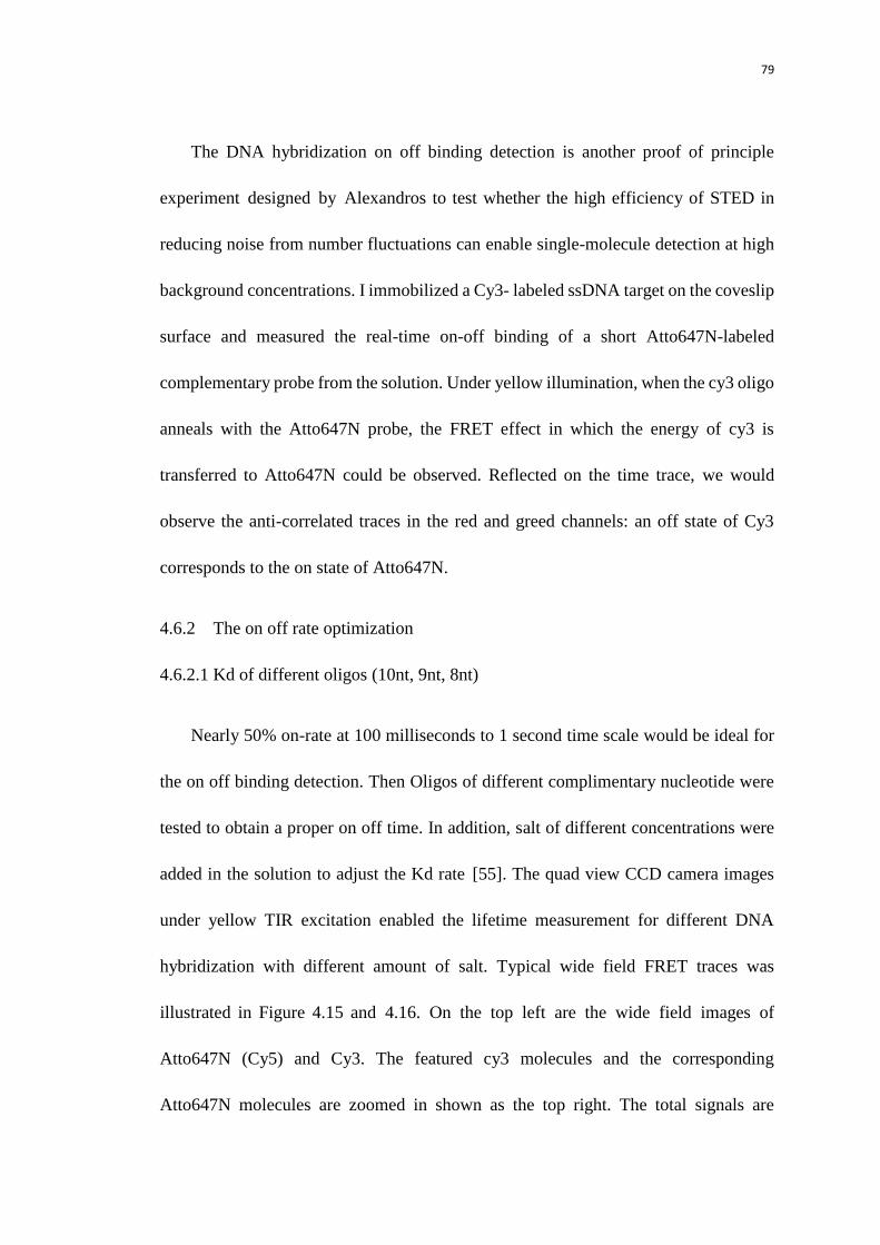
79
The DNA hybridization on off binding detection is another proof of principle
experiment designed by Alexandros to test whether the high efficiency of STED in
reducing noise from number fluctuations can enable single-molecule detection at high
background concentrations. I immobilized a Cy3- labeled ssDNA target on the coveslip
surface and measured the real-time on-off binding of a short Atto647N-labeled
complementary probe from the solution. Under yellow illumination, when the cy3 oligo
anneals with the Atto647N probe, the FRET effect in which the energy of cy3 is
transferred to Atto647N could be observed. Reflected on the time trace, we would
observe the anti-correlated traces in the red and greed channels: an off state of Cy3
corresponds to the on state of Atto647N.
4.6.2 The on off rate optimization
4.6.2.1 Kd of different oligos (10nt, 9nt, 8nt)
Nearly 50% on-rate at 100 milliseconds to 1 second time scale would be ideal for
the on off binding detection. Then Oligos of different complimentary nucleotide were
tested to obtain a proper on off time. In addition, salt of different concentrations were
added in the solution to adjust the Kd rate [55]. The quad view CCD camera images
under yellow TIR excitation enabled the lifetime measurement for different DNA
hybridization with different amount of salt. Typical wide field FRET traces was
illustrated in Figure 4.15 and 4.16. On the top left are the wide field images of
Atto647N (Cy5) and Cy3. The featured cy3 molecules and the corresponding
Atto647N molecules are zoomed in shown as the top right. The total signals are
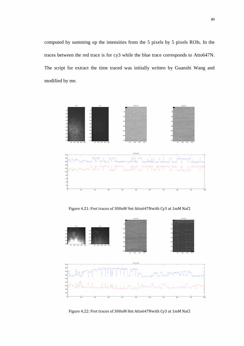
80
computed by summing up the intensities from the 5 pixels by 5 pixels ROIs. In the
traces between the red trace is for cy3 while the blue trace corresponds to Atto647N.
The script for extract the time traced was initially written by Guanshi Wang and
modified by me.
Figure 4.21: Fret traces of 300nM 9nt Atto647Nwith Cy3 at 1mM NaCl
Figure 4.22: Fret traces of 300nM 8nt Atto647Nwith Cy3 at 1mM NaCl
cy5
50 100 150 200 250
50
100
150
200
250
300
350
400
450
500
cy3
50 100 150 200 250
50
100
150
200
250
300
350
400
450
500
cy5 ft 81
50 100 150 200
50
100
150
200
250
300
350
cy3 ft 81
50 100 150 200
50
100
150
200
250
300
350
0 100 200 300 400 500 600 700 800 900 10000
20
40
60
80
100
120
140
160
180
200r-cy3 b-cy5
cy5
50 100 150 200 250
50
100
150
200
250
cy3
50 100 150 200 250
50
100
150
200
250
cy5 ft 85
50 100 150 200
50
100
150
200
250
300
350
cy3 ft 85
50 100 150 200
50
100
150
200
250
300
350
0 100 200 300 400 500 600 700 800 900 10000
100
200
300
400
500
600
700
800
900r-cy3 b-cy5
81
4.6.2.2 Adjust the Kd with NaCl at different concentrations
It turned out that 8nt oligo the imaging buffer contained a variable concentration
of NaCl (750, 500 and 100 µM NaCl for 300, 600 and 1000 nM probe respectively)
would achieve ~50:50 on-off binding equilibrium of the probe to the target
4.6.3 Map the yellow channel and red channel
For the wide field images, the 100nm beads were used for registration. For
extracting traces from images, firstly the cy3 was featured and intensity was
calculated by summation of the ROI with a radius of 3 pixels. Secondly, the intensity
of Atto647N was calculated by adding up the corresponding region in the red channel.
For the STED images, the cy3-Atto647N duplex was utilized. The scanned
images of the colocalized duplex in yellow and red with\without STED provided
information about the offset between them, which later was referred to bring the
molecule at the minimum of STED doughnuts.
4.6.4 Interlace the yellow laser and red laser
The function generator sent two pulses with roughly 180 degree phase difference
to trigger the red laser and the shutter that blocked the yellow laser. The interlaced
yellow and red excitation time trace in Atto647N solution was examined to optimize
the phase shift. The direct excitation trace from red laser and Fret trace were separated
by the 1ms bin time trace, from which the 50Hz yellow excitation period could be
identified, shown in Figure 4.17.

82
Figure 4.23: the time traces in red (top) and yellow channel (bottom) under interlaced red and
yellow excitation.
4.6.5 Take time traces with the interlaced yellow and red laser w/wo STED
Based on the image of the Cy3 and calibrated offset, I managed to center the
target molecule in the excitation peak/zero STED. As the Cy3 and Atto647N dyes
come in close proximity upon duplex DNA formation, I employed the time-interlaced
561nm and 642nm laser beams to detect binding events through Cy3-Atto647N
fluorescence-resonance- energy-transfer (FRET) and direct Atto647N excitation
respectively. Typically, a 40 second trace was taken in which the first 20 seconds
there was no STED and the remaining 20 seconds the STED was turned on.
4.6.6 Data analysis
4.6.6.1 Separate the direct red excitation and FRET traces
0 10 20 30 40 50 60 70 80 90 1000.5
1
1.5
2
2.5x 10
4
time(0.001s)
Photo
n C
ounts
0 10 20 30 40 50 60 70 80 90 10080
100
120
140
160
180
200
time(0.001s)
Photo
n C
ounts

83
The time data was saved in binary file through Picoharp. In matlab, the time
traces were extracted with 1ms time bin size. Next, the direct red excitation and Fret
traces were separated based on the periodical intensity changes, similar to Figure 4.23.
In the following, the corresponding signals were selected and rebinned to 20
milliseconds or the multiple times of 20 milliseconds. In this way, I was able to
measure the FRET and direct excitation simultaneously.
4.6.6.2 SNR of the direct excitation traces with/without STED
The anti-correlated Fret traces could help identify when the hybridization took
place. Thus, I could compare the SNR for this on off hybridization events.
Remarkably, I could recognize the on off events with STED shown in Figure 4.24
drawn by Alexandros. Meanwhile, without STED the binding events were too noisy
to be identified. Real-time traces of directly excited Atto647N revealed noisy intensity
fluctuations, while application of STED resulted in markedly improved SNR,
enabling unambiguous identification of binding events under direct excitation. The
SNR improvements at 100nM, 300nM, 600nM were investigated. 2-3 fold SNR
improvement were achieved with 200mW xy and 500-700mW z doughnut beam.
These results demonstrate that STED can enable single- molecule detection for the
time trace measurement at up to 0.6-1µM solution concentrations. Note that this
approach can also be used to detect transient, weak molecular interactions
(KD~100-1000nM range).
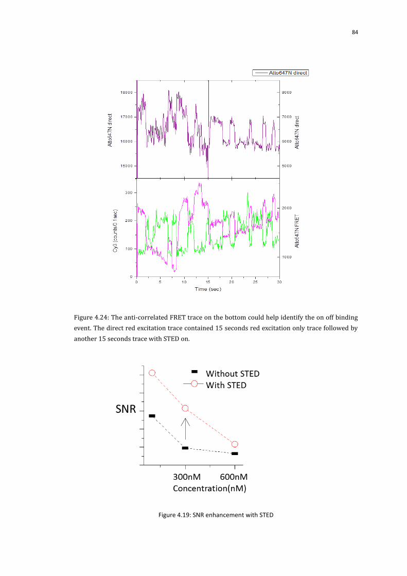
84
Figure 4.24: The anti-correlated FRET trace on the bottom could help identify the on off binding
event. The direct red excitation trace contained 15 seconds red excitation only trace followed by
another 15 seconds trace with STED on.
Figure 4.19: SNR enhancement with STED

85
Chapter Five
Single molecule detection for RNA
Polymerase II transcription
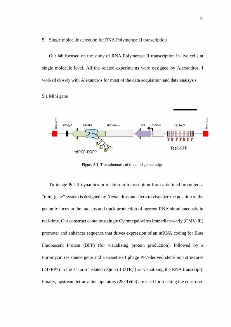
86
5. Single molecule detection for RNA Polymerase II transcription
Our lab focused on the study of RNA Polymerase II transcription in live cells at
single molecule level. All the related experiments were designed by Alexandros. I
worked closely with Alexandros for most of the data acquisition and data analsysis.
5.1 Mini gene
Figure 5.1: The schematic of the mini gene design
To image Pol II dynamics in relation to transcription from a defined promoter, a
“mini-gene” system is designed by Alexandros and Jieru to visualize the position of the
genomic locus in the nucleus and track production of nascent RNA simultaneously in
real-time. Our construct contains a single Cytomegalovirus immediate-early (CMV-IE)
promoter and enhancer sequence that drives expression of an mRNA coding for Blue
Fluorescent Protein (BFP) (for visualizing protein production), followed by a
Puromycin resistance gene and a cassette of phage PP7-derived stem-loop structures
(24×PP7) in the 3‟ un-translated region (3‟UTR) (for visualizing the RNA transcript).
Finally, upstream tetracycline operators (28×TetO) are used for tracking the construct.
Insu
lato
r
Insu
lato
r
SV40pA 24×PP7 IRES-Puro BFP CMV-IE 28×TetO
tdPCP-EGFP TetR-RFP
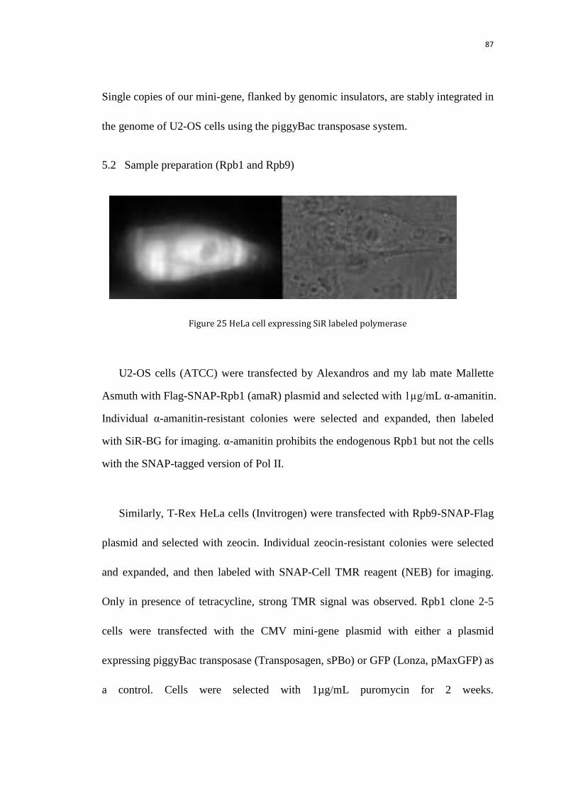
87
Single copies of our mini-gene, flanked by genomic insulators, are stably integrated in
the genome of U2-OS cells using the piggyBac transposase system.
5.2 Sample preparation (Rpb1 and Rpb9)
Figure 25 HeLa cell expressing SiR labeled polymerase
U2-OS cells (ATCC) were transfected by Alexandros and my lab mate Mallette
Asmuth with Flag-SNAP-Rpb1 (amaR) plasmid and selected with 1µg/mL α-amanitin.
Individual α-amanitin-resistant colonies were selected and expanded, then labeled
with SiR-BG for imaging. α-amanitin prohibits the endogenous Rpb1 but not the cells
with the SNAP-tagged version of Pol II.
Similarly, T-Rex HeLa cells (Invitrogen) were transfected with Rpb9-SNAP-Flag
plasmid and selected with zeocin. Individual zeocin-resistant colonies were selected
and expanded, and then labeled with SNAP-Cell TMR reagent (NEB) for imaging.
Only in presence of tetracycline, strong TMR signal was observed. Rpb1 clone 2-5
cells were transfected with the CMV mini-gene plasmid with either a plasmid
expressing piggyBac transposase (Transposagen, sPBo) or GFP (Lonza, pMaxGFP) as
a control. Cells were selected with 1µg/mL puromycin for 2 weeks.
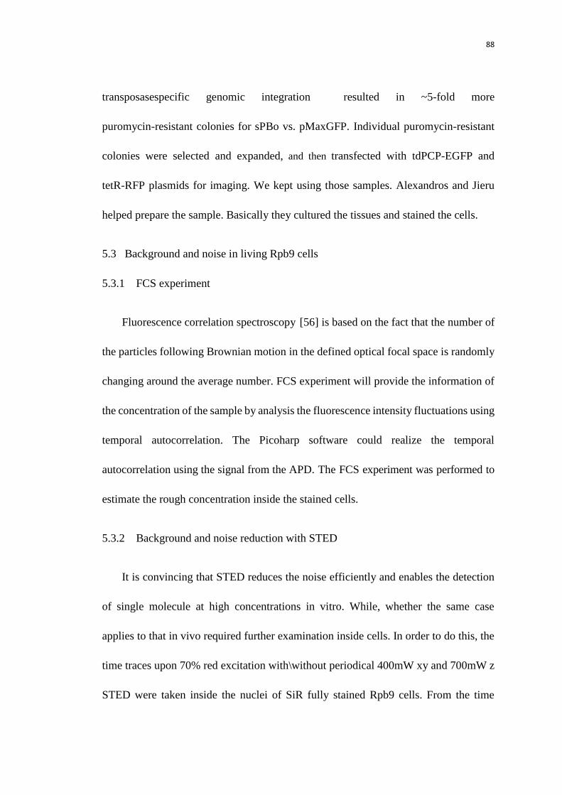
88
transposasespecific genomic integration resulted in ~5-fold more
puromycin-resistant colonies for sPBo vs. pMaxGFP. Individual puromycin-resistant
colonies were selected and expanded, and then transfected with tdPCP-EGFP and
tetR-RFP plasmids for imaging. We kept using those samples. Alexandros and Jieru
helped prepare the sample. Basically they cultured the tissues and stained the cells.
5.3 Background and noise in living Rpb9 cells
5.3.1 FCS experiment
Fluorescence correlation spectroscopy [56] is based on the fact that the number of
the particles following Brownian motion in the defined optical focal space is randomly
changing around the average number. FCS experiment will provide the information of
the concentration of the sample by analysis the fluorescence intensity fluctuations using
temporal autocorrelation. The Picoharp software could realize the temporal
autocorrelation using the signal from the APD. The FCS experiment was performed to
estimate the rough concentration inside the stained cells.
5.3.2 Background and noise reduction with STED
It is convincing that STED reduces the noise efficiently and enables the detection
of single molecule at high concentrations in vitro. While, whether the same case
applies to that in vivo required further examination inside cells. In order to do this, the
time traces upon 70% red excitation with\without periodical 400mW xy and 700mW z
STED were taken inside the nuclei of SiR fully stained Rpb9 cells. From the time

89
trace in Figure 5.3, we have a sense that the noise was suppressed efficiently with
STED.
Figure 5.3: Time trace inside the Rpb9 cell stained with SiR. The STED was on after about 30
seconds.
By adjusting the amount of SiR dyes for the Staining, we could harvest cells
labeled with SiR at different concentrations. Furthermore, even with the same staining
condition, the cells would be characterized with a variety of background level. Hence,
We adopted two concentrations for the staining and ended up with a range of
background levels. The noise reduction was proportional to the background level
reduction in Figure 5.4 drawn by Alexandros, basically the same as in vitro. With
400mW xy and 700mW z STED, the SNR would improve by 3-4 folds, in agreement
with the results from the in vitro solutions. The time traces were measured close to the
center of the nuclei, ensured by looking at the images on the side port camera. Firstly,
the image of cells was centered in xy and the beam was focus on the surface by
moving the stage. Secondly, the stage was moved up 2-3um based on the estimation
0 1000 2000 3000 4000 5000 6000200
400
600
800
1000
1200
1400
1600
time(0.01s)
Cou
nts
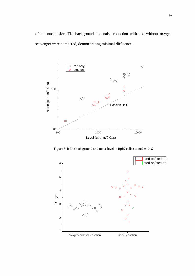
90
of the nuclei size. The background and noise reduction with and without oxygen
scavenger were compared, demonstrating minimal difference.
100 1000 10000
10
100
red only
sted on
No
ise
(co
un
ts/0
.01
s)
Level (counts/0.01s)
Possion limit
Figure 5.4: The background and noise level in Rpb9 cells stained with S
background level reduction noise reduction
1
2
3
4
5
6
Ra
ng
e
sted on/sted off
sted on/sted off
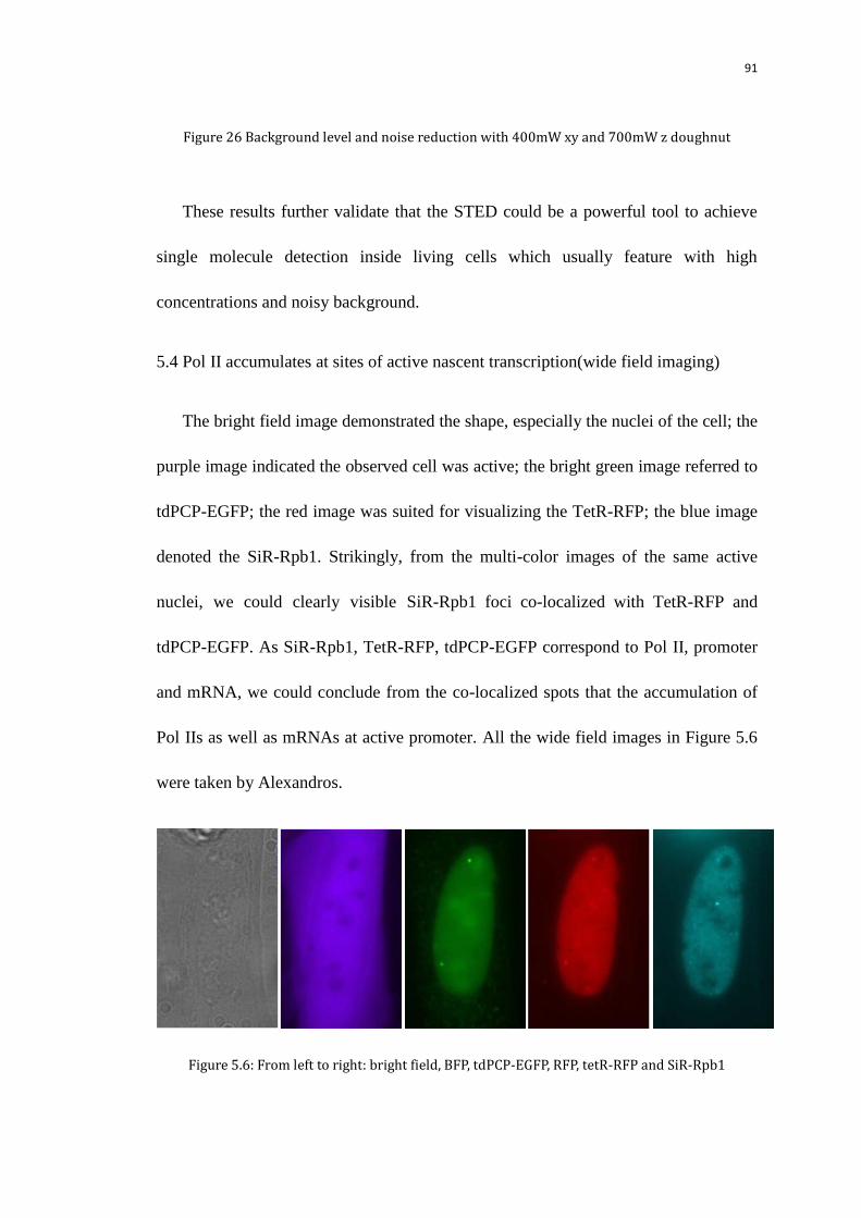
91
Figure 26 Background level and noise reduction with 400mW xy and 700mW z doughnut
These results further validate that the STED could be a powerful tool to achieve
single molecule detection inside living cells which usually feature with high
concentrations and noisy background.
5.4 Pol II accumulates at sites of active nascent transcription(wide field imaging)
The bright field image demonstrated the shape, especially the nuclei of the cell; the
purple image indicated the observed cell was active; the bright green image referred to
tdPCP-EGFP; the red image was suited for visualizing the TetR-RFP; the blue image
denoted the SiR-Rpb1. Strikingly, from the multi-color images of the same active
nuclei, we could clearly visible SiR-Rpb1 foci co-localized with TetR-RFP and
tdPCP-EGFP. As SiR-Rpb1, TetR-RFP, tdPCP-EGFP correspond to Pol II, promoter
and mRNA, we could conclude from the co-localized spots that the accumulation of
Pol IIs as well as mRNAs at active promoter. All the wide field images in Figure 5.6
were taken by Alexandros.
Figure 5.6: From left to right: bright field, BFP, tdPCP-EGFP, RFP, tetR-RFP and SiR-Rpb1

92
5.5 Studying the Pol II using STED setup (methods)
5.5.1 STED alignment
To align the setup, first of all, the beams needed to be overlapped. The same
procedure as before, a dense layer of Atto647N molecules was prepared to align the
APD. The position of the APD was optimized by maximizing its count rate. Then the
xz scanning images help examine and align the z doughnut. Similarly, the immobile
single Atto647N on the PEG coverslip was scanned in xy to optimize the xy doughnut.
With the beams overlapped, the PBS was placed to reflect the emitted fluorescence to
the CCD camera. The PBS was adjusted to ensure the emission not to reach the edge
of field of view based on the reflected beam from the gold coverslip or the
fluorescence of Atto647N solution. Next, the focus on the CCD camera was localized
by maximizing the brightness of single immobile Atto647N. The focus of red
excitation beam and the minimum of the STED beams could be obtained and usually
they should be nearly at the same place. Once the minimum of the STED beams were
known, a single Atto647N was brought to the minimum with the STED periodically
on to quantify the remaining signal. Typically, at least 80% signal would remain with
100mw xy and 400mw z doughnut, seen in figure 5.7.
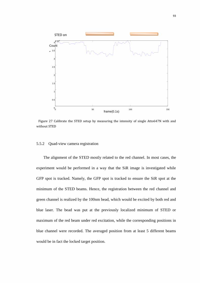
93
Figure 27 Calibrate the STED setup by measuring the intensity of single Atto647N with and
without STED
5.5.2 Quad-view camera registration
The alignment of the STED mostly related to the red channel. In most cases, the
experiment would be performed in a way that the SiR image is investigated while
GFP spot is tracked. Namely, the GFP spot is tracked to ensure the SiR spot at the
minimum of the STED beams. Hence, the registration between the red channel and
green channel is realized by the 100nm bead, which would be excited by both red and
blue laser. The bead was put at the previously localized minimum of STED or
maximum of the red beam under red excitation, while the corresponding positions in
blue channel were recorded. The averaged position from at least 5 different beams
would be in fact the locked target position.
0 50 100 150 0
0.5
1
1.5
2
2.5
3
3.5
4 x 10 4
frame(0.1s)
Count
s
STED on
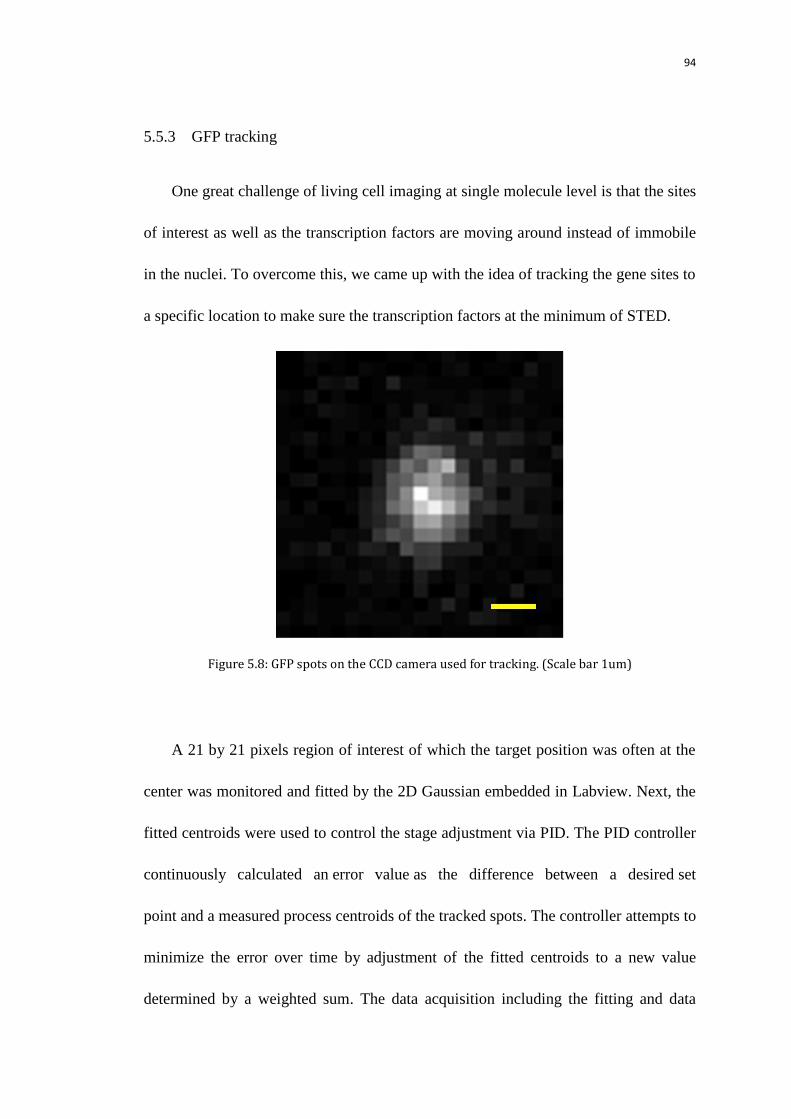
94
5.5.3 GFP tracking
One great challenge of living cell imaging at single molecule level is that the sites
of interest as well as the transcription factors are moving around instead of immobile
in the nuclei. To overcome this, we came up with the idea of tracking the gene sites to
a specific location to make sure the transcription factors at the minimum of STED.
Figure 5.8: GFP spots on the CCD camera used for tracking. (Scale bar 1um)
A 21 by 21 pixels region of interest of which the target position was often at the
center was monitored and fitted by the 2D Gaussian embedded in Labview. Next, the
fitted centroids were used to control the stage adjustment via PID. The PID controller
continuously calculated an error value as the difference between a desired set
point and a measured process centroids of the tracked spots. The controller attempts to
minimize the error over time by adjustment of the fitted centroids to a new value
determined by a weighted sum. The data acquisition including the fitting and data
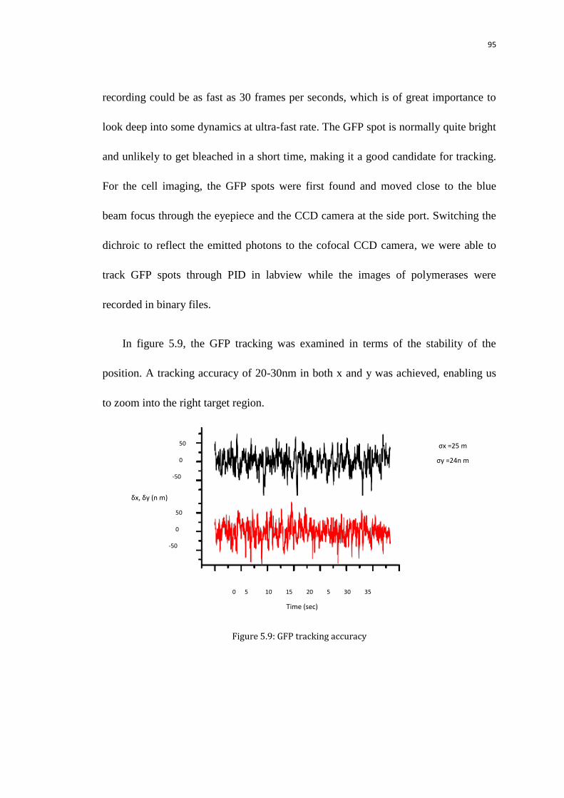
95
recording could be as fast as 30 frames per seconds, which is of great importance to
look deep into some dynamics at ultra-fast rate. The GFP spot is normally quite bright
and unlikely to get bleached in a short time, making it a good candidate for tracking.
For the cell imaging, the GFP spots were first found and moved close to the blue
beam focus through the eyepiece and the CCD camera at the side port. Switching the
dichroic to reflect the emitted photons to the cofocal CCD camera, we were able to
track GFP spots through PID in labview while the images of polymerases were
recorded in binary files.
In figure 5.9, the GFP tracking was examined in terms of the stability of the
position. A tracking accuracy of 20-30nm in both x and y was achieved, enabling us
to zoom into the right target region.
Figure 5.9: GFP tracking accuracy
δx, δy (n m)
50
0
-50
0 5 10 15 20 5 30 35
Time (sec)
σx =25 m
σy =24n m
50
0
-50
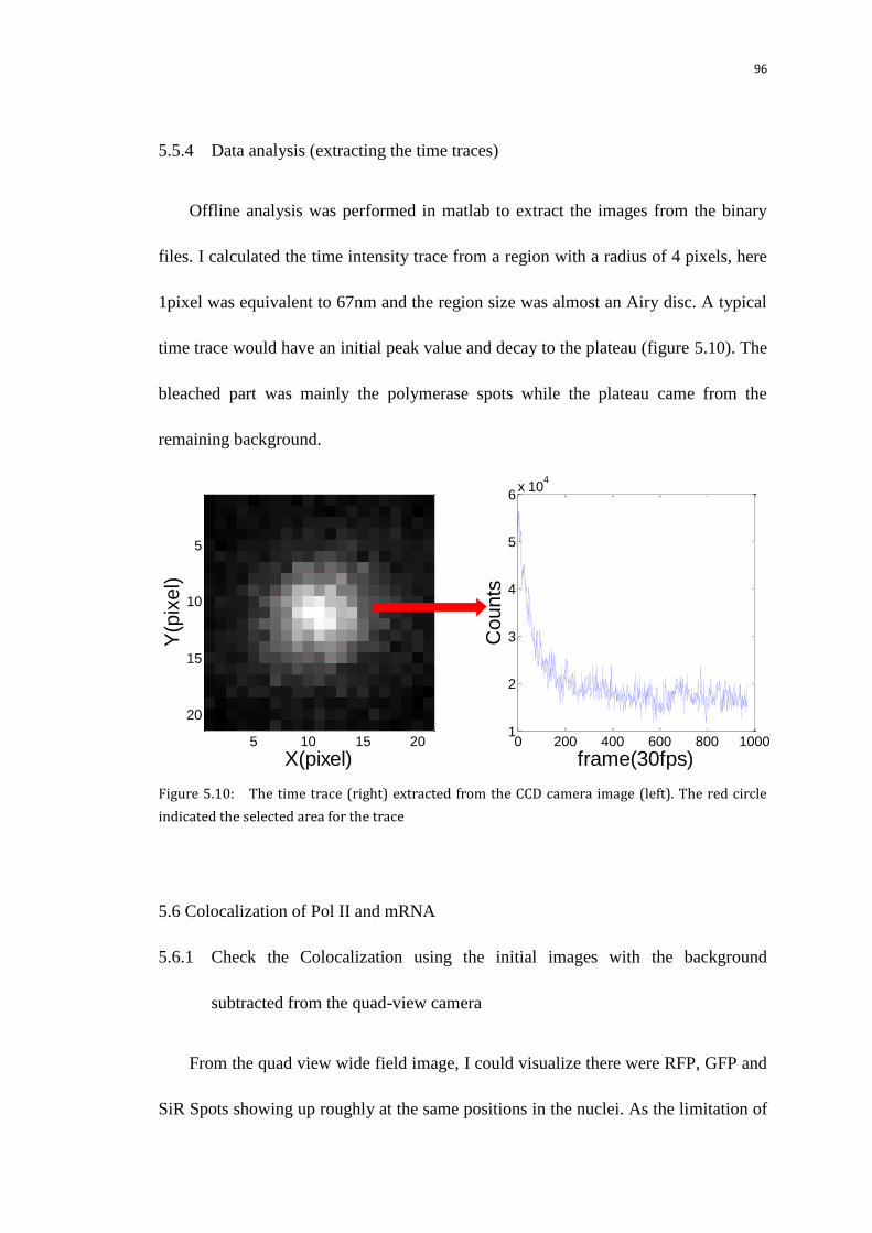
96
5.5.4 Data analysis (extracting the time traces)
Offline analysis was performed in matlab to extract the images from the binary
files. I calculated the time intensity trace from a region with a radius of 4 pixels, here
1pixel was equivalent to 67nm and the region size was almost an Airy disc. A typical
time trace would have an initial peak value and decay to the plateau (figure 5.10). The
bleached part was mainly the polymerase spots while the plateau came from the
remaining background.
Figure 5.10: The time trace (right) extracted from the CCD camera image (left). The red circle
indicated the selected area for the trace
5.6 Colocalization of Pol II and mRNA
5.6.1 Check the Colocalization using the initial images with the background
subtracted from the quad-view camera
From the quad view wide field image, I could visualize there were RFP, GFP and
SiR Spots showing up roughly at the same positions in the nuclei. As the limitation of
X(pixel)
Y(p
ixel)
5 10 15 20
5
10
15
20
0 200 400 600 800 10001
2
3
4
5
6x 10
4
frame(30fps)
Counts
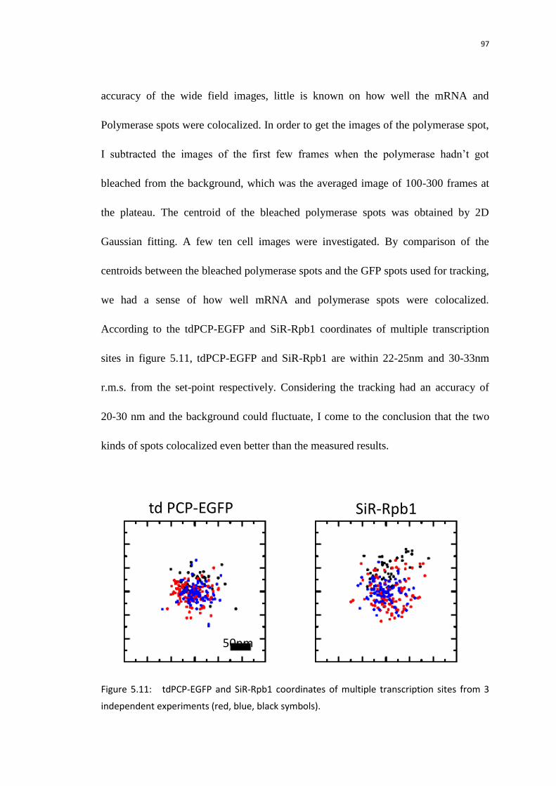
97
accuracy of the wide field images, little is known on how well the mRNA and
Polymerase spots were colocalized. In order to get the images of the polymerase spot,
I subtracted the images of the first few frames when the polymerase hadn‟t got
bleached from the background, which was the averaged image of 100-300 frames at
the plateau. The centroid of the bleached polymerase spots was obtained by 2D
Gaussian fitting. A few ten cell images were investigated. By comparison of the
centroids between the bleached polymerase spots and the GFP spots used for tracking,
we had a sense of how well mRNA and polymerase spots were colocalized.
According to the tdPCP-EGFP and SiR-Rpb1 coordinates of multiple transcription
sites in figure 5.11, tdPCP-EGFP and SiR-Rpb1 are within 22-25nm and 30-33nm
r.m.s. from the set-point respectively. Considering the tracking had an accuracy of
20-30 nm and the background could fluctuate, I come to the conclusion that the two
kinds of spots colocalized even better than the measured results.
Figure 5.11: tdPCP-EGFP and SiR-Rpb1 coordinates of multiple transcription sites from 3
independent experiments (red, blue, black symbols).
td PCP-EGFP SiR-Rpb1
50nm

98
5.6.2 Check the Colocalization by direct 3D scanning images.
5.6.2.1 Find the GFP spots and roughly center the spots.
The eyepiece and wide field images provided a large field of view to help find
and roughly locate the spots. With the 50:50 beam splitter that split the emitted
fluorescence, half to the APDs and half to the CCD camera, we were able to easily
switch between the cofocal CCD quad view image and the scanning cofocal image
using APD. The spots were moved to the predefined position by checking the GFP
images on the CCD camera. Next, as scanning starting point located at (6um, 1um)
based on the trajectory the stage was moved in x by 6um and in y by1 um so that the
spot would be roughly centered at the scanned regions.
5.6.2.2 3D real time imaging using FPGA
To directly visualize the colocalization between GFP and SiR spots, a 2by2um
region was scanned in 0.2 second and after each scanning the stage moved in z by a
500nm step.
The signals from the two APDs, together with the markers from E712, were
transferred to FPGA in which the online analysis could be performed simultaneously.
In total, 5 frames were scanned in the space. The 3D cofocal images in figure 5.12
demonstrated how the GFP spot and SiR spot looked like

99
Figure 5.12: The two color cofocal scanning images in 3D. 2umby2um in xy and 0.5um step size in
z. The pixel size is 40nm.
One out of the five frames closest to the best focus was selected. In the case of
figure 5.12, the forth frame was selected. Both a selected 9 by 9 pixel (1pixel =40nm)
regions containing the GFP and SiR spots from that frame were fitted with 2D
Gaussian. Relative xy coordinates of tdPCP-EGFP and SiR-Rpb1 from n=42 images
reached to the similar conclusion that the mRNA and Polymerase spots were
colocalized within 50-60nm. We shall notice that the fitted results would be noisy
partially because the background was not homogonous inside the cells, especially for
the polymerases.
blue frame 1 (z = -1um)
20 40
10
20
30
40
50
red frame 1
20 40
10
20
30
40
50
blue frame 2 (z = -0.5um)
20 40
10
20
30
40
50
red frame 2
20 40
10
20
30
40
50
blue frame 3 (z = 0um)
20 40
10
20
30
40
50
red frame 3
20 40
10
20
30
40
50
blue frame 4 (z = 0.5um)
20 40
10
20
30
40
50
red frame 4
20 40
10
20
30
40
50
blue frame 5 (z = 1um)
20 40
10
20
30
40
50
red frame 5
20 40
10
20
30
40
50
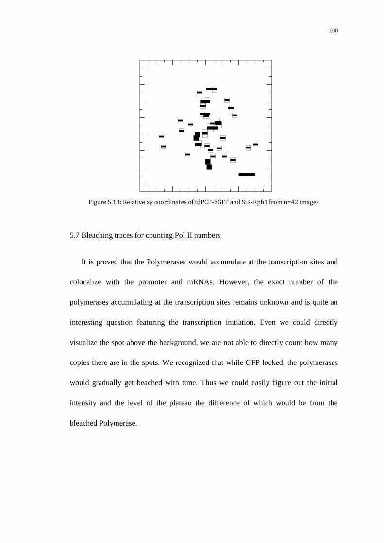
100
Figure 5.13: Relative xy coordinates of tdPCP-EGFP and SiR-Rpb1 from n=42 images
5.7 Bleaching traces for counting Pol II numbers
It is proved that the Polymerases would accumulate at the transcription sites and
colocalize with the promoter and mRNAs. However, the exact number of the
polymerases accumulating at the transcription sites remains unknown and is quite an
interesting question featuring the transcription initiation. Even we could directly
visualize the spot above the background, we are not able to directly count how many
copies there are in the spots. We recognized that while GFP locked, the polymerases
would gradually get beached with time. Thus we could easily figure out the initial
intensity and the level of the plateau the difference of which would be from the
bleached Polymerase.

101
5.7.1 Calibrate the step size of the bleaching time traces using less stained sample
The intensity of single Polymerase was calibrated using the less stained cell
samples, which was 20-25% of maximal SiR staining level. For less stained cells, the
background was lower and less noisy, and intensity traces usually contained one or
two step event.
Figure 5.14: Time trace from less stained sample with red only
Signal
(A.U.)
100 200
1200
1000
800
600
400
200
red only
20-25% labeled
Time(100ms)
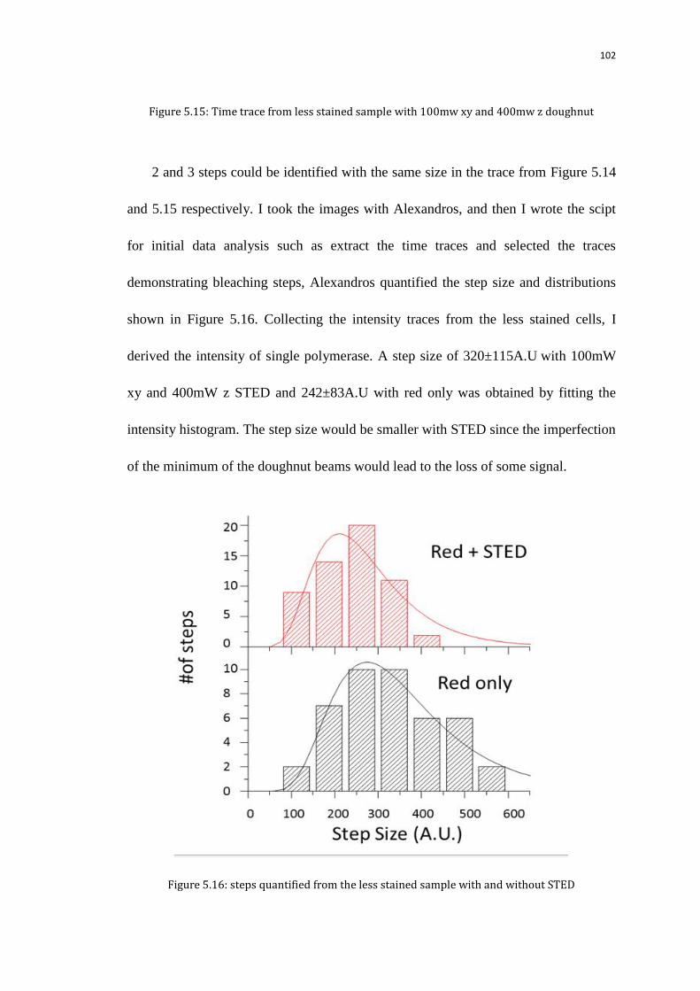
102
Figure 5.15: Time trace from less stained sample with 100mw xy and 400mw z doughnut
2 and 3 steps could be identified with the same size in the trace from Figure 5.14
and 5.15 respectively. I took the images with Alexandros, and then I wrote the scipt
for initial data analysis such as extract the time traces and selected the traces
demonstrating bleaching steps, Alexandros quantified the step size and distributions
shown in Figure 5.16. Collecting the intensity traces from the less stained cells, I
derived the intensity of single polymerase. A step size of 320±115A.U with 100mW
xy and 400mW z STED and 242±83A.U with red only was obtained by fitting the
intensity histogram. The step size would be smaller with STED since the imperfection
of the minimum of the doughnut beams would lead to the loss of some signal.
Figure 5.16: steps quantified from the less stained sample with and without STED
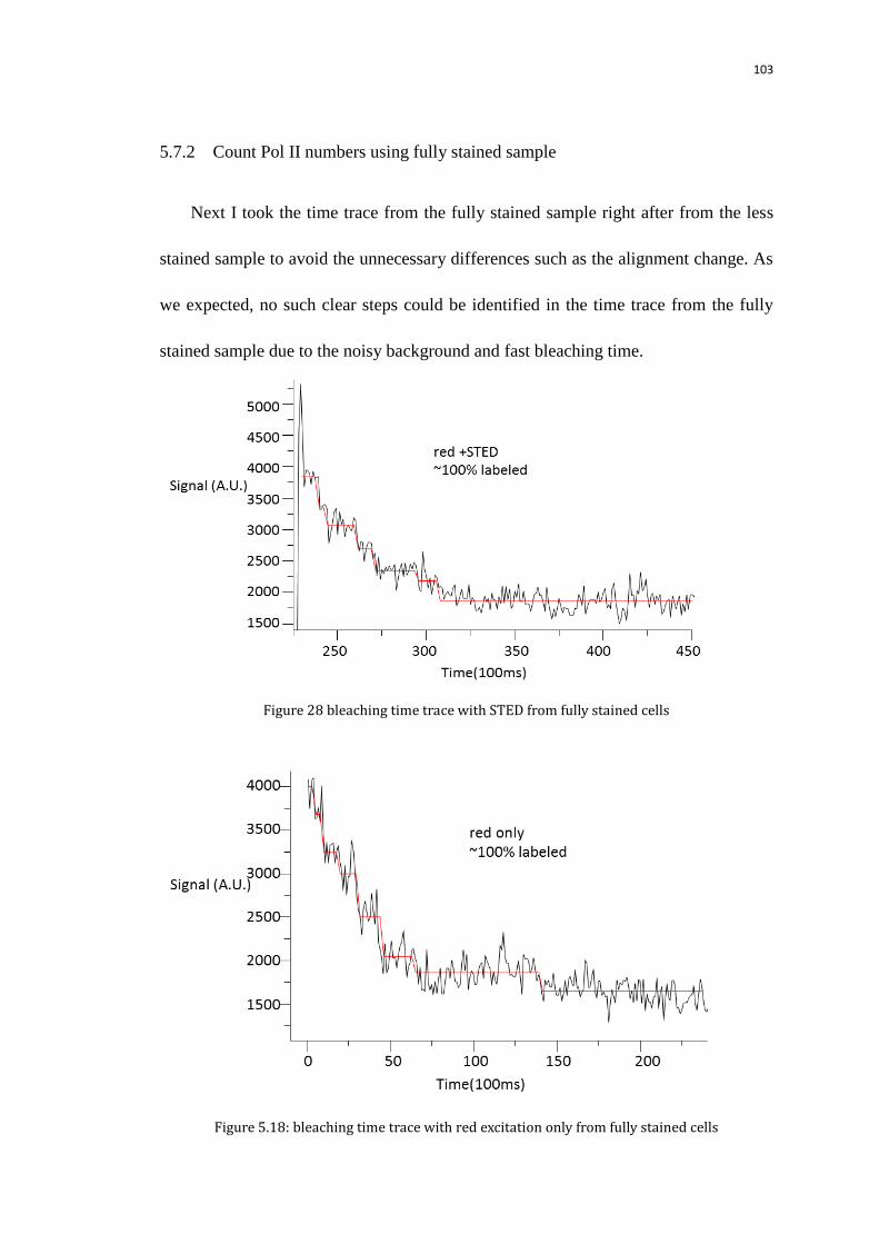
103
5.7.2 Count Pol II numbers using fully stained sample
Next I took the time trace from the fully stained sample right after from the less
stained sample to avoid the unnecessary differences such as the alignment change. As
we expected, no such clear steps could be identified in the time trace from the fully
stained sample due to the noisy background and fast bleaching time.
Figure 28 bleaching time trace with STED from fully stained cells
Figure 5.18: bleaching time trace with red excitation only from fully stained cells
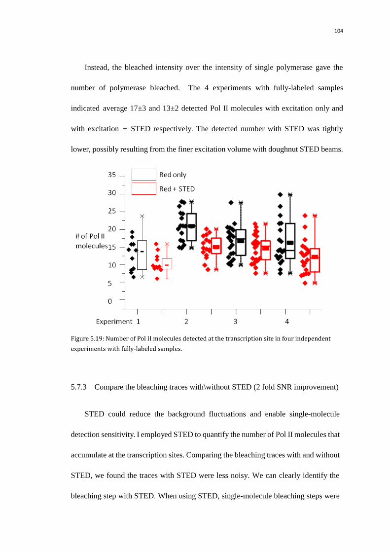
104
Instead, the bleached intensity over the intensity of single polymerase gave the
number of polymerase bleached. The 4 experiments with fully-labeled samples
indicated average 17±3 and 13±2 detected Pol II molecules with excitation only and
with excitation + STED respectively. The detected number with STED was tightly
lower, possibly resulting from the finer excitation volume with doughnut STED beams.
Figure 5.19: Number of Pol II molecules detected at the transcription site in four independent
experiments with fully-labeled samples.
5.7.3 Compare the bleaching traces with\without STED (2 fold SNR improvement)
STED could reduce the background fluctuations and enable single-molecule
detection sensitivity. I employed STED to quantify the number of Pol II molecules that
accumulate at the transcription sites. Comparing the bleaching traces with and without
STED, we found the traces with STED were less noisy. We can clearly identify the
bleaching step with STED. When using STED, single-molecule bleaching steps were
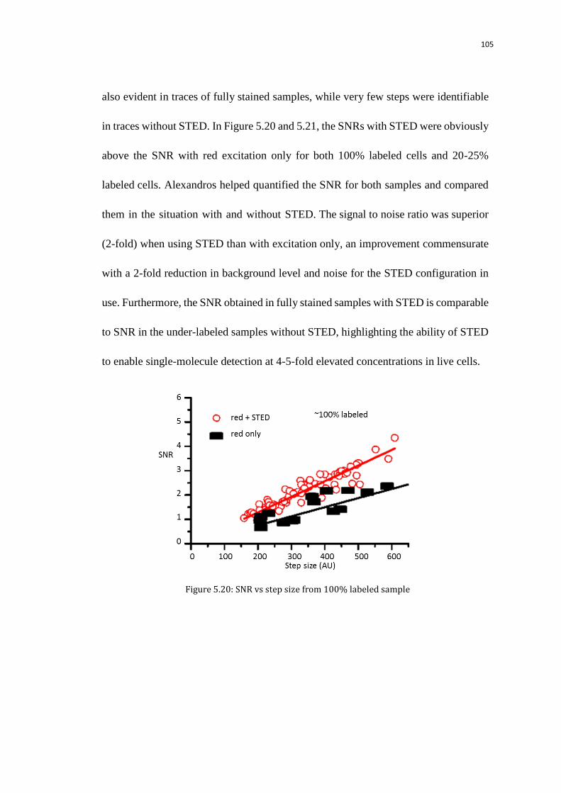
105
also evident in traces of fully stained samples, while very few steps were identifiable
in traces without STED. In Figure 5.20 and 5.21, the SNRs with STED were obviously
above the SNR with red excitation only for both 100% labeled cells and 20-25%
labeled cells. Alexandros helped quantified the SNR for both samples and compared
them in the situation with and without STED. The signal to noise ratio was superior
(2-fold) when using STED than with excitation only, an improvement commensurate
with a 2-fold reduction in background level and noise for the STED configuration in
use. Furthermore, the SNR obtained in fully stained samples with STED is comparable
to SNR in the under-labeled samples without STED, highlighting the ability of STED
to enable single-molecule detection at 4-5-fold elevated concentrations in live cells.
Figure 5.20: SNR vs step size from 100% labeled sample
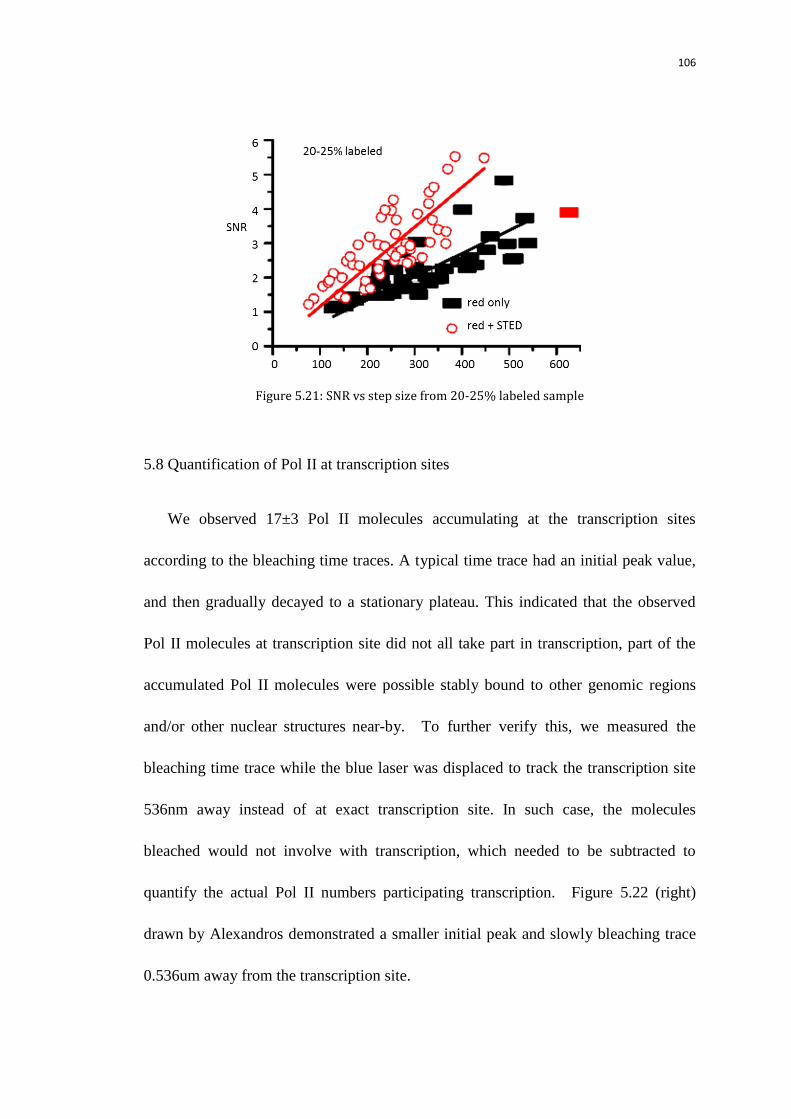
106
Figure 5.21: SNR vs step size from 20-25% labeled sample
5.8 Quantification of Pol II at transcription sites
We observed 17±3 Pol II molecules accumulating at the transcription sites
according to the bleaching time traces. A typical time trace had an initial peak value,
and then gradually decayed to a stationary plateau. This indicated that the observed
Pol II molecules at transcription site did not all take part in transcription, part of the
accumulated Pol II molecules were possible stably bound to other genomic regions
and/or other nuclear structures near-by. To further verify this, we measured the
bleaching time trace while the blue laser was displaced to track the transcription site
536nm away instead of at exact transcription site. In such case, the molecules
bleached would not involve with transcription, which needed to be subtracted to
quantify the actual Pol II numbers participating transcription. Figure 5.22 (right)
drawn by Alexandros demonstrated a smaller initial peak and slowly bleaching trace
0.536um away from the transcription site.
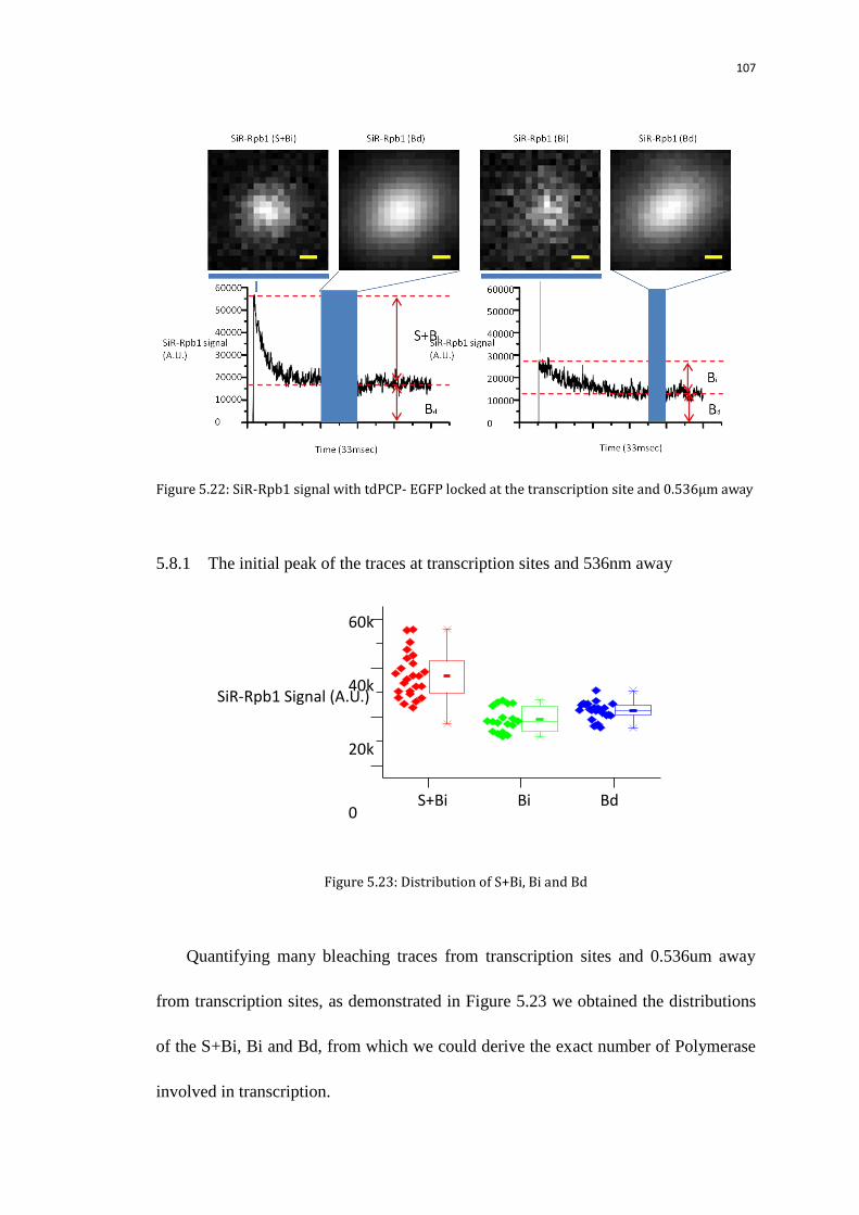
107
Figure 5.22: SiR-Rpb1 signal with tdPCP- EGFP locked at the transcription site and 0.536µm away
5.8.1 The initial peak of the traces at transcription sites and 536nm away
Figure 5.23: Distribution of S+Bi, Bi and Bd
Quantifying many bleaching traces from transcription sites and 0.536um away
from transcription sites, as demonstrated in Figure 5.23 we obtained the distributions
of the S+Bi, Bi and Bd, from which we could derive the exact number of Polymerase
involved in transcription.
SiR-Rpb1 Signal (A.U.)
S+Bi Bi Bd
60k
40k
20k
0
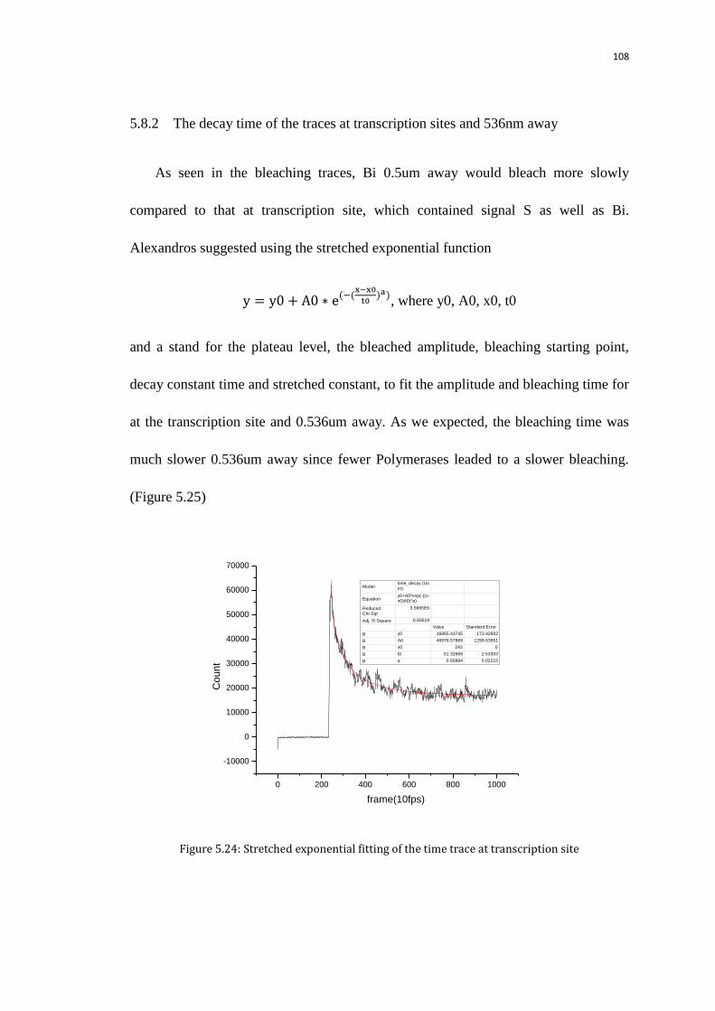
108
5.8.2 The decay time of the traces at transcription sites and 536nm away
As seen in the bleaching traces, Bi 0.5um away would bleach more slowly
compared to that at transcription site, which contained signal S as well as Bi.
Alexandros suggested using the stretched exponential function
e
, where y0, A0, x0, t0
and a stand for the plateau level, the bleached amplitude, bleaching starting point,
decay constant time and stretched constant, to fit the amplitude and bleaching time for
at the transcription site and 0.536um away. As we expected, the bleaching time was
much slower 0.536um away since fewer Polymerases leaded to a slower bleaching.
(Figure 5.25)
0 200 400 600 800 1000
-10000
0
10000
20000
30000
40000
50000
60000
70000
Co
un
t
frame(10fps)
Modeltime_decay (User)
Equationy0+A0*exp(-((x-x0)/t0)^a)
Reduced Chi-Sqr
3.5665E6
Adj. R-Square 0.93519
Value Standard Error
B y0 16865.43745 173.42802
B A0 46976.57869 1299.63951
B x0 243 0
B t0 51.32669 2.53303
B a 0.60984 0.02215
Figure 5.24: Stretched exponential fitting of the time trace at transcription site
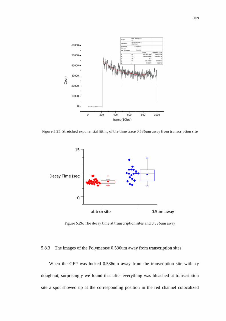
109
0 200 400 600 800 1000
0
10000
20000
30000
40000
50000
60000
Co
un
t
frame(10fps)
Modeltime_decay (User)
Equationy0+A0*exp(-((x-x0)/t0)^a)
Reduced Chi-Sqr
7.56335E6
Adj. R-Square 0.64982
Value Standard Error
B y0 30316.87899 466.32286
B A0 14694.84446 1060.42146
B x0 218 0
B t0 196.17923 14.77932
B a 0.98909 0.12062
Figure 5.25: Stretched exponential fitting of the time trace 0.536um away from transcription site
Figure 5.26: The decay time at transcription sites and 0.536um away
5.8.3 The images of the Polymerase 0.536um away from transcription sites
When the GFP was locked 0.536um away from the transcription site with xy
doughnut, surprisingly we found that after everything was bleached at transcription
site a spot showed up at the corresponding position in the red channel colocalized
Decay Time (sec)
at trxn site 0.5um away
15
0
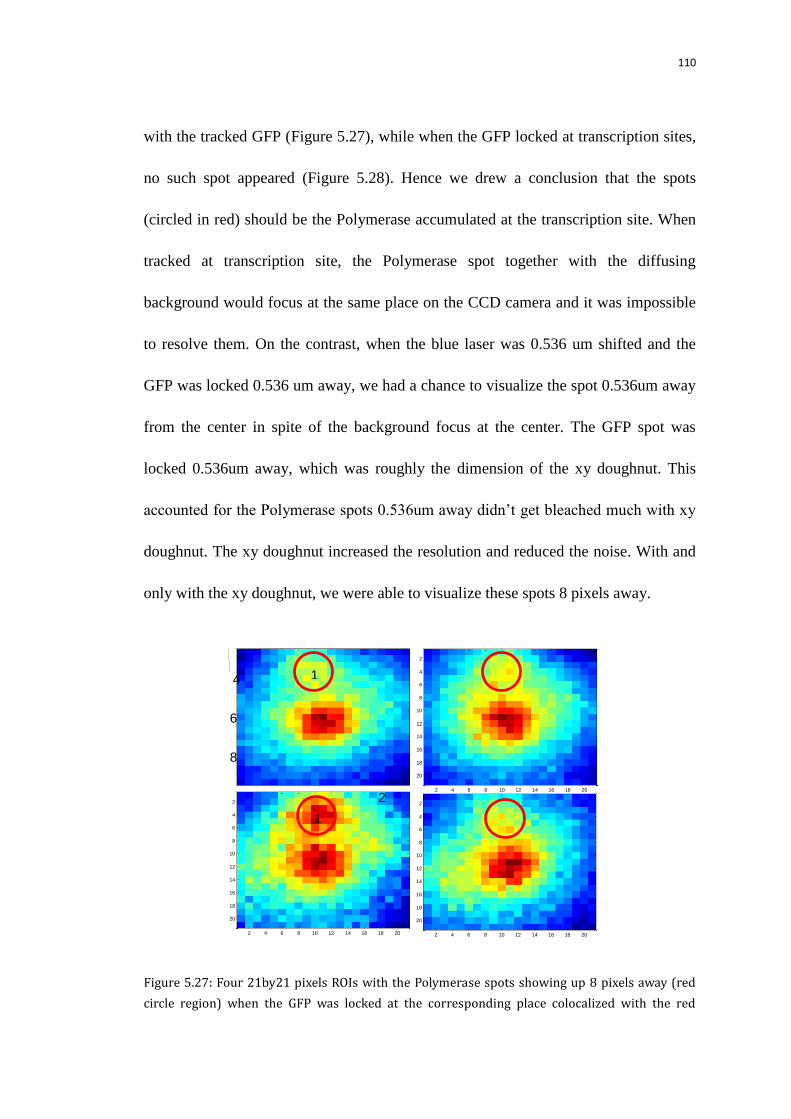
110
with the tracked GFP (Figure 5.27), while when the GFP locked at transcription sites,
no such spot appeared (Figure 5.28). Hence we drew a conclusion that the spots
(circled in red) should be the Polymerase accumulated at the transcription site. When
tracked at transcription site, the Polymerase spot together with the diffusing
background would focus at the same place on the CCD camera and it was impossible
to resolve them. On the contrast, when the blue laser was 0.536 um shifted and the
GFP was locked 0.536 um away, we had a chance to visualize the spot 0.536um away
from the center in spite of the background focus at the center. The GFP spot was
locked 0.536um away, which was roughly the dimension of the xy doughnut. This
accounted for the Polymerase spots 0.536um away didn‟t get bleached much with xy
doughnut. The xy doughnut increased the resolution and reduced the noise. With and
only with the xy doughnut, we were able to visualize these spots 8 pixels away.
Figure 5.27: Four 21by21 pixels ROIs with the Polymerase spots showing up 8 pixels away (red
circle region) when the GFP was locked at the corresponding place colocalized with the red
2 4 6 8 10 12 14 16 18 20
2
4
6
8
10
12
14
16
18
20
2 4 6 8 10 12 14 16 18 20
2
4
6
8
10
12
14
16
18
20
2 4 6 8 10 12 14 16 18 20
2
4
6
8
10
12
14
16
18
20
2
4 6 8
1
1

111
circled region after bleaching.
Figure 5.28: Four 21by21 pixels ROIs when the GFP was locked at transcription site after
bleaching
5.8.4 The actual Pol II numbers involved in transcription
Comparing the bleaching traces at transcription sites and 536nm away from the
transcription sites, we observed that the initial peak 536nm away from the
transcription sites was roughly 1/3 that at the transcription sites and the decay time
was slower, indicating: (i) the SiR-Rpb1 signal from the transcription site consists of
67±1.6% Pol II accumulating at the mini-gene (S) and 33±1.6% immobile background
(Bi); (ii) the total Pol II background consists of 37±3.5% immobile (Bi) and 63±3.5%
diffusing (Bd) background (mean±SD, n=3 experiments, >10 transcription sites each).

112
5.9 Size of the Pol II spots at transcription sites
Next, as we concluded roughly 10 Pol II involved with transcription at the sites,
we wondered in which way these Pol II were organized. Measuring the sizes of these
Pol II spots would give some information in terms of this question.
At certain circumstances, a cylindrical lens would be set before the CCD camera
to realize 3D tracking. The orientation of the cylindrical lens was adjusted to
introduce additional phase in x axis. To verify this, the image of a bead or a molecule
was indeed elongated in one axis. Figure 5.29 demonstrated the σx , σy at different z
places and the σx /σy was no longer roughly 1 at all z positions, instead the σx /σy
would be sensitive to the z position. The parameter of σx /σy could be set to a fixed
value via PID to track the object in a fixed z positions, usually the focal plane. With
the cylindrical lens, I repeated the calibration and got the results shown in Figure
5.30.
Comparing the (σx, σy) distributions of the Pol II spots with that of the beads, we
found that the distributions of the Pol II spots were quite spreading even with STED,
making it difficult to quantify the sizes of the Pol II spots. This is not surprising as the
fitting of the images over very noise background would be quite noisy even the
averaged background was subtracted. In addition, the tracking held an accuracy of
roughly 30nm. What‟s more, the images could be from out of focus, resulting in the

113
blurring of the images. All these proved that it was not a decent way to quantify the
sizes by 2D Gauss fitting of the images with averaged background subtracted.
5.9.1 Measure the sizes of the initial images with the background subtracted from
the quad-view camera referring to nanoparticle size calibration
As mentioned before, we could visualize the images on the quad-view CCD
camera. By subtracting the averaged background from the stationary plateau part, we
ended up with the images of the bleached Pol II. At the condition of 10 fps or 30 fps
acquisition rate and 6.7uW excitation power, the Pol II usually lasted a few frames
before they started getting bleached. Then we were able to obtain the size of these
images by 2D Gauss fitting. In order to relate the sizes of the images on the quad view
CCD camera to the actual sizes of the Pol II spots, we calibrated the image sizes of
100nm, 200nm and 500nm beads as well as single immobile Atto647N molecules.
The beads were bound on the glass coverslip nonspecifically. The bead was found and
centered in xy, and then was placed 500nm or 1umbelow the focus. I tried taking data
for 2000 frame at a frame rate of 10 fps and 30 fps. The stage was move up by 50nm
or 100nm every 50 frames. While data acquisition, the images were fitted using 2D
Gauss in labview and the parameters were saved in matlab. In the end, we obtained
the σx and σy of the bead images at different focal planes. For each size, the images
of 6 beads were acquired. And the (σx , σy) distributions were very similar from bead
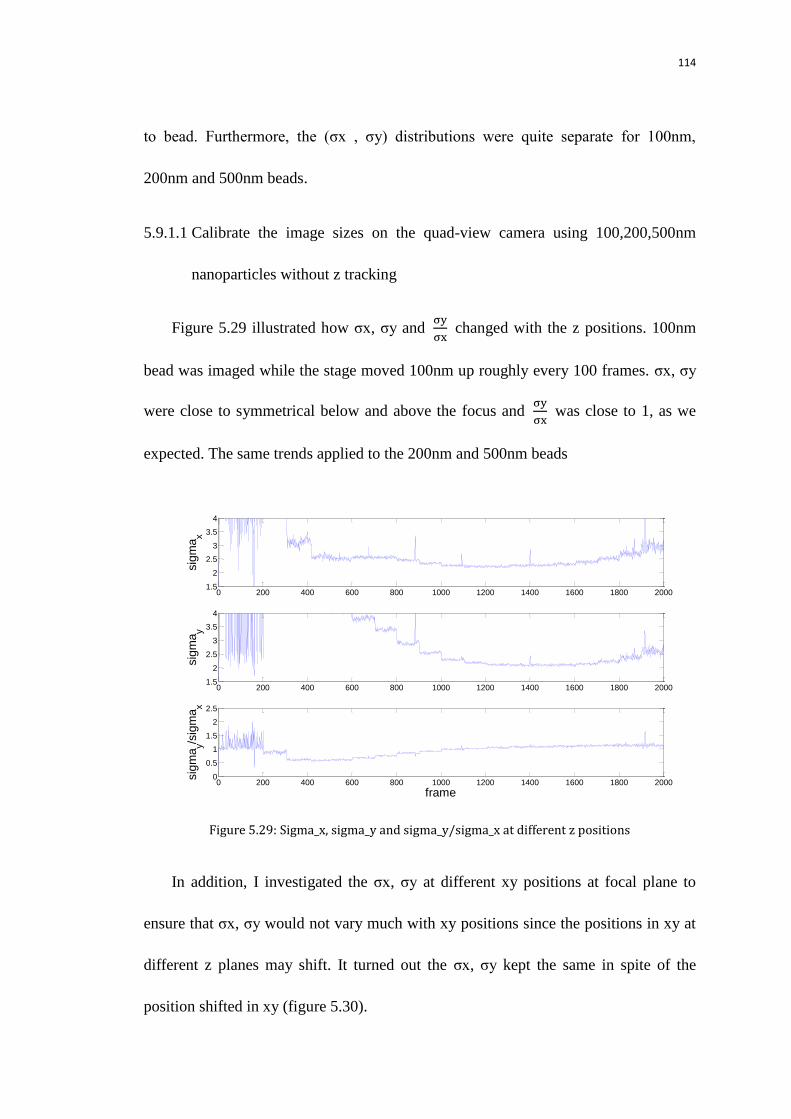
114
to bead. Furthermore, the (σx , σy) distributions were quite separate for 100nm,
200nm and 500nm beads.
5.9.1.1 Calibrate the image sizes on the quad-view camera using 100,200,500nm
nanoparticles without z tracking
Figure 5.29 illustrated how σx, σy and
changed with the z positions. 100nm
bead was imaged while the stage moved 100nm up roughly every 100 frames. σx, σy
were close to symmetrical below and above the focus and
was close to 1, as we
expected. The same trends applied to the 200nm and 500nm beads
Figure 5.29: Sigma_x, sigma_y and sigma_y/sigma_x at different z positions
In addition, I investigated the σx, σy at different xy positions at focal plane to
ensure that σx, σy would not vary much with xy positions since the positions in xy at
different z planes may shift. It turned out the σx, σy kept the same in spite of the
position shifted in xy (figure 5.30).
0 200 400 600 800 1000 1200 1400 1600 1800 20001.5
2
2.5
3
3.5
4
sig
ma
x
0 200 400 600 800 1000 1200 1400 1600 1800 20001.5
2
2.5
3
3.5
4
sig
ma
y
0 200 400 600 800 1000 1200 1400 1600 1800 20000
0.5
1
1.5
2
2.5
frame
sig
ma
y/sig
ma
x
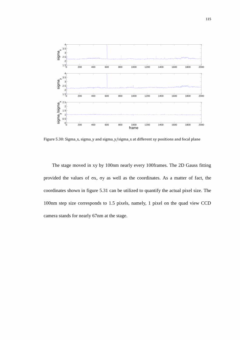
115
Figure 5.30: Sigma_x, sigma_y and sigma_y/sigma_x at different xy positions and focal plane
The stage moved in xy by 100nm nearly every 100frames. The 2D Gauss fitting
provided the values of σx, σy as well as the coordinates. As a matter of fact, the
coordinates shown in figure 5.31 can be utilized to quantify the actual pixel size. The
100nm step size corresponds to 1.5 pixels, namely, 1 pixel on the quad view CCD
camera stands for nearly 67nm at the stage.
0 200 400 600 800 1000 1200 1400 1600 1800 20001.5
2
2.5
3
3.5
4
sig
ma
x
0 200 400 600 800 1000 1200 1400 1600 1800 20001.5
2
2.5
3
3.5
4
sig
ma
y
0 200 400 600 800 1000 1200 1400 1600 1800 20000
0.5
1
1.5
2
2.5
frame
sig
ma
y/sig
ma
x
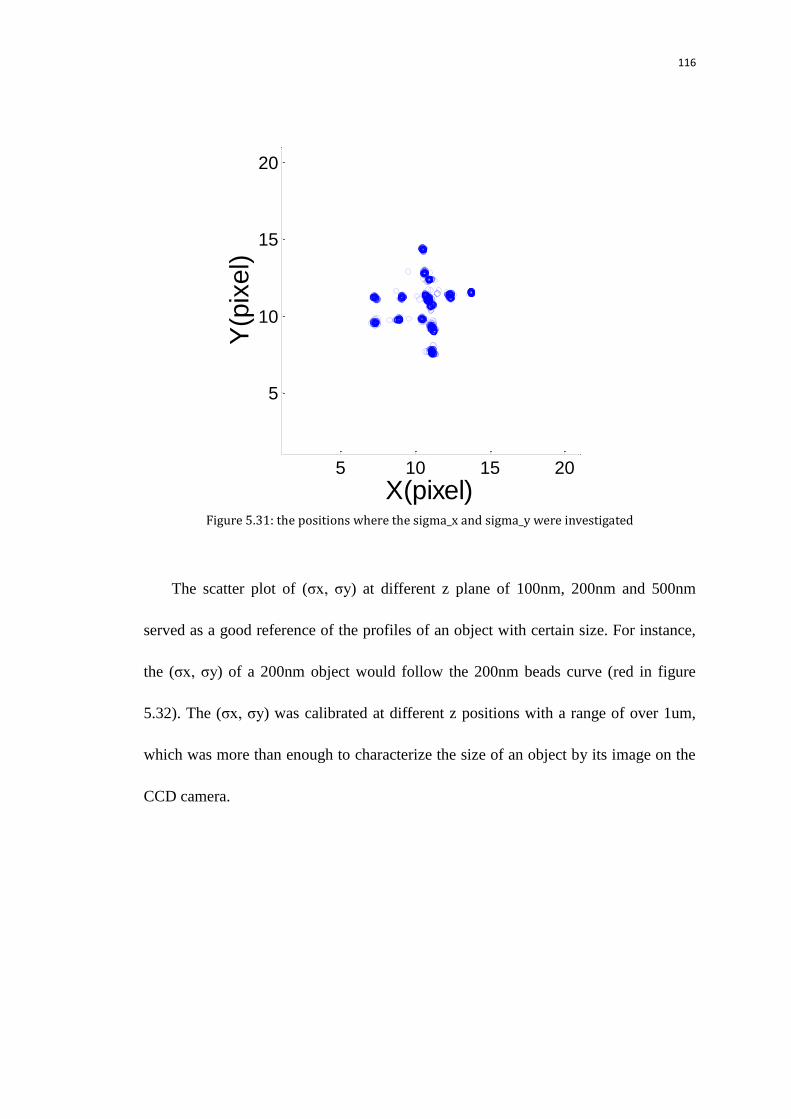
116
Figure 5.31: the positions where the sigma_x and sigma_y were investigated
The scatter plot of (σx, σy) at different z plane of 100nm, 200nm and 500nm
served as a good reference of the profiles of an object with certain size. For instance,
the (σx, σy) of a 200nm object would follow the 200nm beads curve (red in figure
5.32). The (σx, σy) was calibrated at different z positions with a range of over 1um,
which was more than enough to characterize the size of an object by its image on the
CCD camera.
5 10 15 20
5
10
15
20
X(pixel)
Y(p
ixel)

117
Figure 5.32: (sigma_x, sigma_y) of 100nm 200nm and 500nm beads at different z
5.9.1.2 Calibrate the image sizes on the quad-view camera using 100,200,500nm
nanoparticles with z tracking
At certain circumstances, a cylindrical lens would be set before the CCD camera
to realize 3D tracking. The orientation of the cylindrical lens was adjusted to
introduce additional phase in x axis or in y axis. The image of a bead or a molecule
was ensured to be elongated in one axis. Figure 5.33 demonstrated the σx , σy at
different z places and the σx /σy was no longer roughly 1 at all z positions, instead the
σx /σy would be sensitive to the z position.
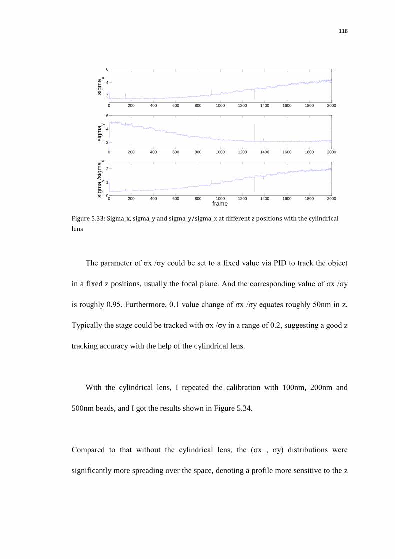
118
Figure 5.33: Sigma_x, sigma_y and sigma_y/sigma_x at different z positions with the cylindrical
lens
The parameter of σx /σy could be set to a fixed value via PID to track the object
in a fixed z positions, usually the focal plane. And the corresponding value of σx /σy
is roughly 0.95. Furthermore, 0.1 value change of σx /σy equates roughly 50nm in z.
Typically the stage could be tracked with σx /σy in a range of 0.2, suggesting a good z
tracking accuracy with the help of the cylindrical lens.
With the cylindrical lens, I repeated the calibration with 100nm, 200nm and
500nm beads, and I got the results shown in Figure 5.34.
Compared to that without the cylindrical lens, the (σx , σy) distributions were
significantly more spreading over the space, denoting a profile more sensitive to the z
0 200 400 600 800 1000 1200 1400 1600 1800 2000
2
4
6
sig
ma
x
0 200 400 600 800 1000 1200 1400 1600 1800 2000
2
4
6
sig
ma
y
0 200 400 600 800 1000 1200 1400 1600 1800 20000
1
2
frame
sig
ma
y/sig
ma
x
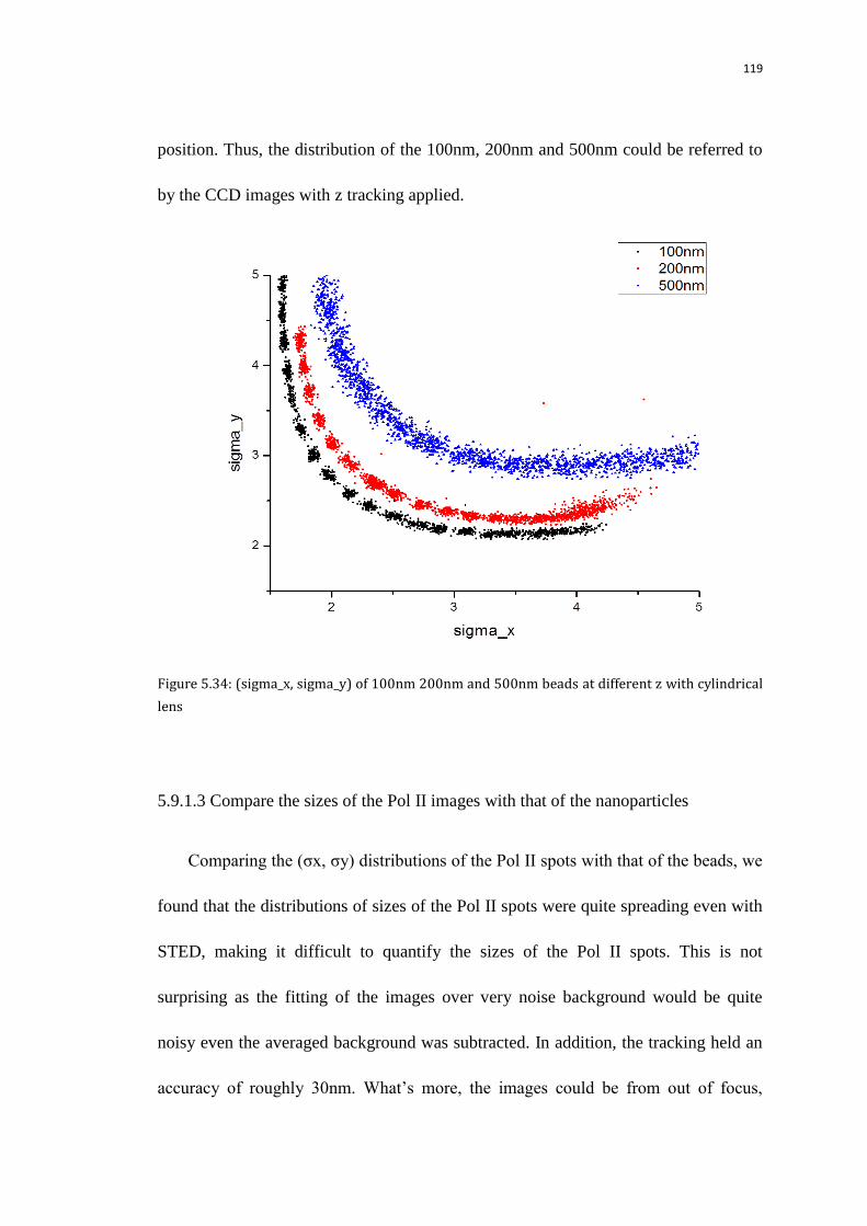
119
position. Thus, the distribution of the 100nm, 200nm and 500nm could be referred to
by the CCD images with z tracking applied.
Figure 5.34: (sigma_x, sigma_y) of 100nm 200nm and 500nm beads at different z with cylindrical
lens
5.9.1.3 Compare the sizes of the Pol II images with that of the nanoparticles
Comparing the (σx, σy) distributions of the Pol II spots with that of the beads, we
found that the distributions of sizes of the Pol II spots were quite spreading even with
STED, making it difficult to quantify the sizes of the Pol II spots. This is not
surprising as the fitting of the images over very noise background would be quite
noisy even the averaged background was subtracted. In addition, the tracking held an
accuracy of roughly 30nm. What‟s more, the images could be from out of focus,
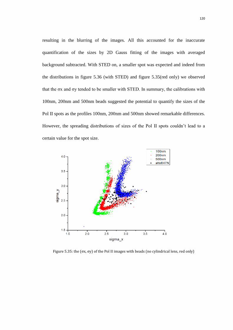
120
resulting in the blurring of the images. All this accounted for the inaccurate
quantification of the sizes by 2D Gauss fitting of the images with averaged
background subtracted. With STED on, a smaller spot was expected and indeed from
the distributions in figure 5.36 (with STED) and figure 5.35(red only) we observed
that the σx and σy tended to be smaller with STED. In summary, the calibrations with
100nm, 200nm and 500nm beads suggested the potential to quantify the sizes of the
Pol II spots as the profiles 100nm, 200nm and 500nm showed remarkable differences.
However, the spreading distributions of sizes of the Pol II spots couldn‟t lead to a
certain value for the spot size.
Figure 5.35: the (σx, σy) of the Pol II images with beads (no cylindrical lens, red only)

121
Figure 5.36: Compare the (σx, σy) of the Pol II images with beads (no cylindrical lens, with STED)
Figure 5.37: compare the (σx, σy) of the Pol II images with beads (with cylindrical lens, red only)

122
5.9.2 Check the sizes of the initial images with the background subtracted from the
quad-view camera with xy doughnut of different power
As we know, the convolution of two Gaussian functions (f, g) is also Gaussian.
And the width of convolution could be described as
√
Assuming that the Pol II spot is Gaussian shaped, the width is denoted
as 𝑜 , the point spread function of the excitation beam is also
approximately Gaussian. Hence we derive the width of the detected images on the
CCD to be
√
Where is the width of the PSF.
The image size could be measured by fitting the background subtracted
image, while could be calibrated with single Atto647N. More importantly, the
effective PSF could be modified by progressively increasing xy doughnut (0 ~
400mW). The scanning images provided us with the widths of the effective PSFs for
0mW, 100mW, 200mW, 400mW xy doughnut, as well as the remaining signal at the
minimum of the doughnut beam. After intense discussion, we adopted this method
brought by Alexandros for quantified the size of Pol II cluster.

123
5.9.2.1 Resolution, Signal remaining with different power xy doughnut
Basically, 2um by 2um regions containing immobile Atto647N molecules were
scanned in 8 seconds with red excitation as well as progressively increasing xy
doughnut. The resolution with 0mW, 100mW, 200mW and 400mW xy doughnut
provided a range of , enabling the fitting of equation
regarding , , In addition, the remaining signals were
calibrated for each STED power by comparing the peak values of the images of the
molecules.
STED power(mW) Resolution sigma(nm) Signal remaining
0 113.221541 1
100 82.10521 0.889349
200 76.63468 0.799906
400 64.8654 0.74167
Table 5.1: Resolution and signal remaining change with STED power
5.9.2.2 Fit the size with calibrated data
With a range of from different xy doughnut and the derived equation, we
could unveil the transcription spot size. The resolution and the signal remaining in
table 2 needed to be included for calculating the actual PSF. Moreover, a (first-order)
correction factor of e
, where =32nm is the r.m.s of the tracking
displacement from the set point, was conducted to compensation of the tracking

124
fluctuation. For each STED power, over 10 transcription sites were measured. Data
from two experiments using clone 5 cells (open symbols) and one experiment using
clone 6 cells (solid symbols) are shown in Figure 5.38. Applying the derived
relationship to the measured and , we estimated the transcription size to be
85±11nm. The data analysis in Figure 5.38 was done by Alexandros.
Figure 5.38: Relative signal (top) and relative background level (bottom) locked at transcription
site with different PSFs
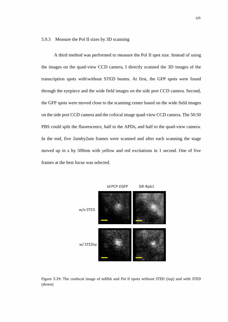
125
5.9.3 Measure the Pol II sizes by 3D scanning
A third method was performed to measure the Pol II spot size. Instead of using
the images on the quad-view CCD camera, I directly scanned the 3D images of the
transcription spots with\without STED beams. At first, the GFP spots were found
through the eyepiece and the wide field images on the side port CCD camera. Second,
the GFP spots were moved close to the scanning center based on the wide field images
on the side port CCD camera and the cofocal image quad-view CCD camera. The 50:50
PBS could split the fluorescence, half to the APDs, and half to the quad-view camera.
In the end, five 2umby2um frames were scanned and after each scanning the stage
moved up in z by 500nm with yellow and red excitations in 1 second. One of five
frames at the best focus was selected.
Figure 5.39: The confocal image of mRNA and Pol II spots without STED (top) and with STED
(down)

126
The colocalized spots were featured and a region of 9 pixels containing the spot
was fitted 2D Gaussian peak functions with sigma s sx, sy and r.m.s. size s was
estimated as √ . Median values are 168nm and 98nm for excitation and
excitation + STEDxy respectively, indicating an r.m.s size strxn site~40-50nm,
according to the equation
. The non-uniform background and the
possible out of focus case leaded to the uncertainty of the results.
Figure 5.40: The fitted SiR sizes with and without STEDxy
5.10 Dynamics of the Pol II transcription cycle at the CMV mini-gene.
In order to investigate the dynamics of the Pol II transcription, the experiments
designed by Alexandros were performed.
5.10.1 Pol II recovery experiment
5.10.1.1 Bleaching the Pol II and retake the bleaching traces after certain minutes
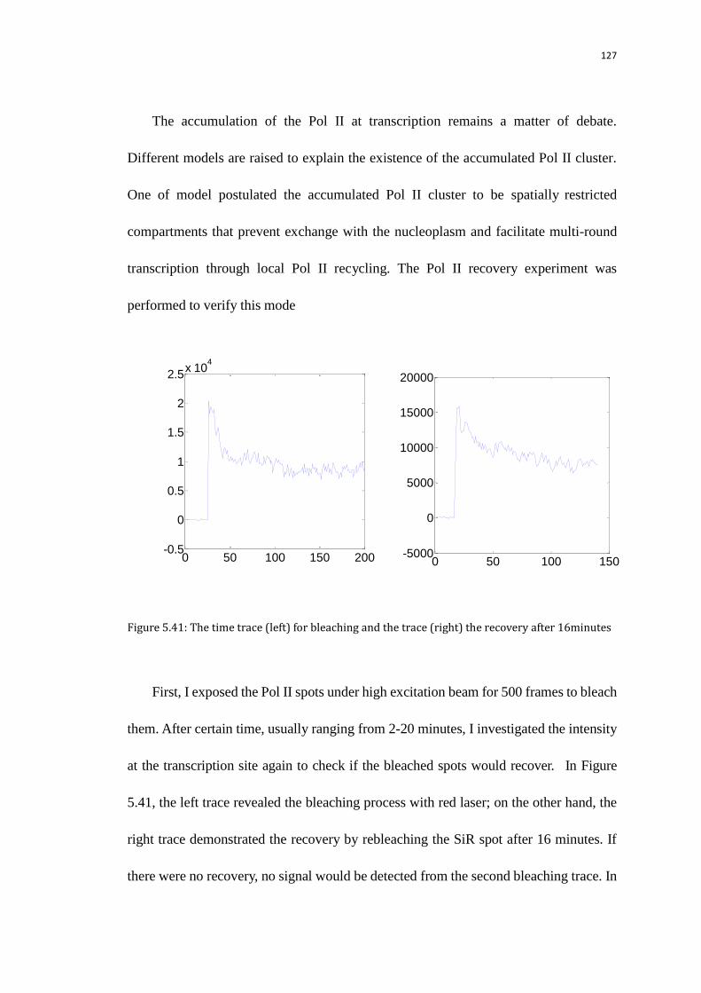
127
The accumulation of the Pol II at transcription remains a matter of debate.
Different models are raised to explain the existence of the accumulated Pol II cluster.
One of model postulated the accumulated Pol II cluster to be spatially restricted
compartments that prevent exchange with the nucleoplasm and facilitate multi-round
transcription through local Pol II recycling. The Pol II recovery experiment was
performed to verify this mode
Figure 5.41: The time trace (left) for bleaching and the trace (right) the recovery after 16minutes
First, I exposed the Pol II spots under high excitation beam for 500 frames to bleach
them. After certain time, usually ranging from 2-20 minutes, I investigated the intensity
at the transcription site again to check if the bleached spots would recover. In Figure
5.41, the left trace revealed the bleaching process with red laser; on the other hand, the
right trace demonstrated the recovery by rebleaching the SiR spot after 16 minutes. If
there were no recovery, no signal would be detected from the second bleaching trace. In
0 50 100 150 200-0.5
0
0.5
1
1.5
2
2.5x 10
4
0 50 100 150-5000
0
5000
10000
15000
20000
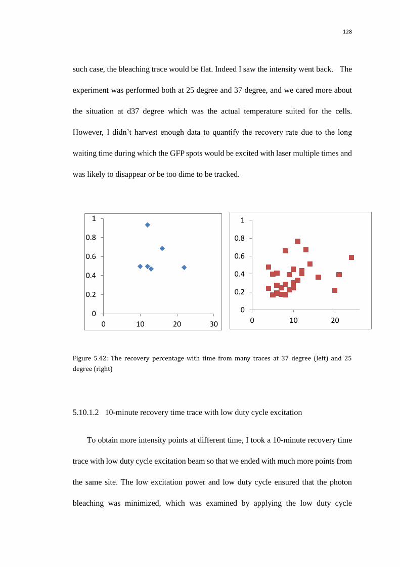
128
such case, the bleaching trace would be flat. Indeed I saw the intensity went back. The
experiment was performed both at 25 degree and 37 degree, and we cared more about
the situation at d37 degree which was the actual temperature suited for the cells.
However, I didn‟t harvest enough data to quantify the recovery rate due to the long
waiting time during which the GFP spots would be excited with laser multiple times and
was likely to disappear or be too dime to be tracked.
Figure 5.42: The recovery percentage with time from many traces at 37 degree (left) and 25
degree (right)
5.10.1.2 10-minute recovery time trace with low duty cycle excitation
To obtain more intensity points at different time, I took a 10-minute recovery time
trace with low duty cycle excitation beam so that we ended with much more points from
the same site. The low excitation power and low duty cycle ensured that the photon
bleaching was minimized, which was examined by applying the low duty cycle
0
0.2
0.4
0.6
0.8
1
0 10 20 30
0
0.2
0.4
0.6
0.8
1
0 10 20
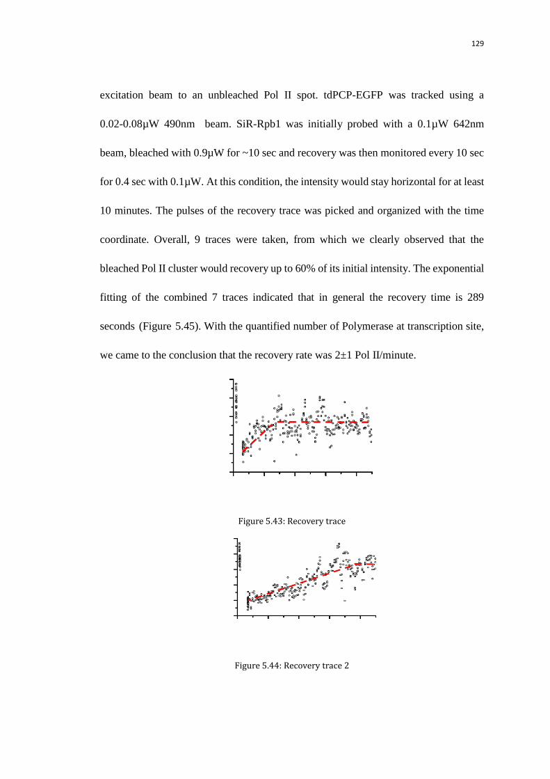
129
excitation beam to an unbleached Pol II spot. tdPCP-EGFP was tracked using a
0.02-0.08µW 490nm beam. SiR-Rpb1 was initially probed with a 0.1µW 642nm
beam, bleached with 0.9µW for ~10 sec and recovery was then monitored every 10 sec
for 0.4 sec with 0.1µW. At this condition, the intensity would stay horizontal for at least
10 minutes. The pulses of the recovery trace was picked and organized with the time
coordinate. Overall, 9 traces were taken, from which we clearly observed that the
bleached Pol II cluster would recovery up to 60% of its initial intensity. The exponential
fitting of the combined 7 traces indicated that in general the recovery time is 289
seconds (Figure 5.45). With the quantified number of Polymerase at transcription site,
we came to the conclusion that the recovery rate was 2±1 Pol II/minute.
Figure 5.43: Recovery trace
Figure 5.44: Recovery trace 2

130
Figure 5.45: exponential fit of 9 recovery trace
5.10.1.3 3D scanning images before and after bleaching as well as after 10-minute
recovery
The 50:50 PBS enabled us to switch between the quad view CCD camera used
for tracking and time trace acquisition and APDs suited for cofocal scanning. For
direct visualization of the recovery, the 3D scanning cofocal images were investigated.
Firstly, we checked the initial image of the SiR spot before we bleached it using high
excitation laser. Secondly, the 3D images were taken right after the bleaching to make
sure that the SiR spots were totally bleached. In the end, after about 8 minutes, we
rescanned the same volume to see if the spot reappeared at the expected. From figure,
we actually saw a spot reappeared colocalized with the GFP spot and at the same
positions as the initial SiR spot, providing substantial evidence the recovery of the Pol II
cluster. The recovery would not take place if the Polymerases were recycling, meaning
the recycling model probably would not stand.
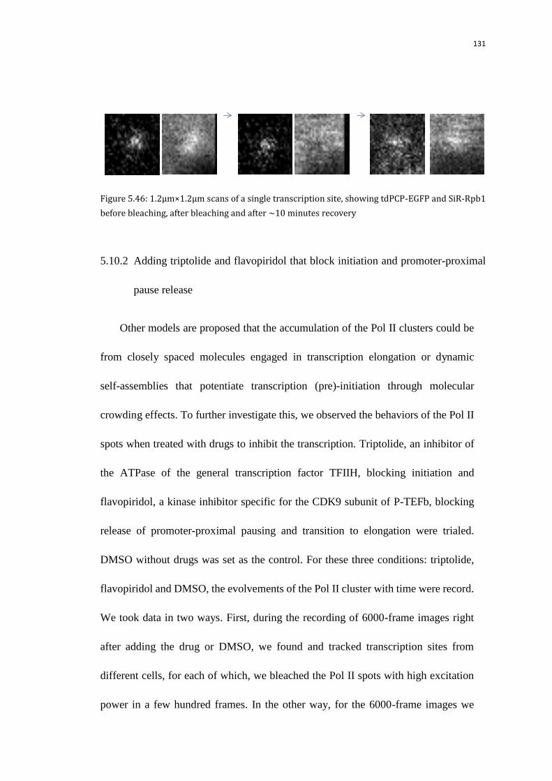
131
Figure 5.46: 1.2µm×1.2µm scans of a single transcription site, showing tdPCP-EGFP and SiR-Rpb1
before bleaching, after bleaching and after ~10 minutes recovery
5.10.2 Adding triptolide and flavopiridol that block initiation and promoter-proximal
pause release
Other models are proposed that the accumulation of the Pol II clusters could be
from closely spaced molecules engaged in transcription elongation or dynamic
self-assemblies that potentiate transcription (pre)-initiation through molecular
crowding effects. To further investigate this, we observed the behaviors of the Pol II
spots when treated with drugs to inhibit the transcription. Triptolide, an inhibitor of
the ATPase of the general transcription factor TFIIH, blocking initiation and
flavopiridol, a kinase inhibitor specific for the CDK9 subunit of P-TEFb, blocking
release of promoter-proximal pausing and transition to elongation were trialed.
DMSO without drugs was set as the control. For these three conditions: triptolide,
flavopiridol and DMSO, the evolvements of the Pol II cluster with time were record.
We took data in two ways. First, during the recording of 6000-frame images right
after adding the drug or DMSO, we found and tracked transcription sites from
different cells, for each of which, we bleached the Pol II spots with high excitation
power in a few hundred frames. In the other way, for the 6000-frame images we
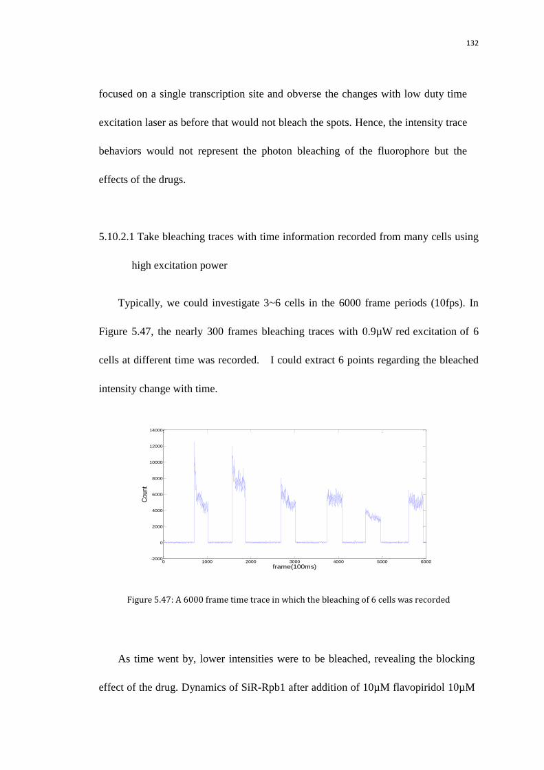
132
focused on a single transcription site and obverse the changes with low duty time
excitation laser as before that would not bleach the spots. Hence, the intensity trace
behaviors would not represent the photon bleaching of the fluorophore but the
effects of the drugs.
5.10.2.1 Take bleaching traces with time information recorded from many cells using
high excitation power
Typically, we could investigate 3~6 cells in the 6000 frame periods (10fps). In
Figure 5.47, the nearly 300 frames bleaching traces with 0.9µW red excitation of 6
cells at different time was recorded. I could extract 6 points regarding the bleached
intensity change with time.
Figure 5.47: A 6000 frame time trace in which the bleaching of 6 cells was recorded
As time went by, lower intensities were to be bleached, revealing the blocking
effect of the drug. Dynamics of SiR-Rpb1 after addition of 10µM flavopiridol 10µM
0 1000 2000 3000 4000 5000 6000-2000
0
2000
4000
6000
8000
10000
12000
14000
frame(100ms)
Cou
nt
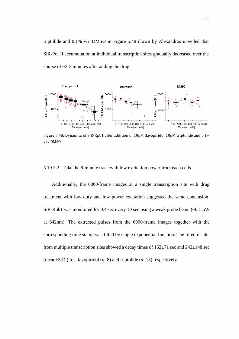
133
triptolide and 0.1% v/v DMSO in Figure 5.48 drawn by Alexandros unveiled that
SiR-Pol II accumulation at individual transcription sites gradually decreased over the
course of ~3-5 minutes after adding the drug.
Figure 5.48: Dynamics of SiR-Rpb1 after addition of 10µM flavopiridol 10µM triptolide and 0.1%
v/v DMSO
5.10.2.2 Take the 8-minute trace with low excitation power from each cells
Additionally, the 6000-frame images at a single transcription site with drug
treatment with low duty and low power excitation suggested the same conclusion.
SiR-Rpb1 was monitored for 0.4 sec every 10 sec using a weak probe beam (~0.1 µW
at 642nm). The extracted pulses from the 6000-frame images together with the
corresponding time stamp was fitted by single exponential function. The fitted results
from multiple transcription sites showed a decay times of 162±71 sec and 242±148 sec
(mean±S.D.) for flavopiridol (n=8) and triptolide (n=15) respectively.

134
Figure 5.49: The decay traces with drug treatment with the GFP locked
Figure 5.50: The fitted decay time from multiple transcription site with drug treatment
5.10.2.3 Data analysis and Conclusion
Based on the intensity traces, the Pol II clusters with drugs disappeared in 3-5
minutes, arguing against a stable pool of immobilized Pol II in a pre- existing nuclear
scaffold or “factory” that persists in the absence of ongoing transcription. The results
also disagree with proposals for molecular crowding effects taking place before
initiation.

135
Bibliography
[1] Abbe, Ernst, "Über einen neuen Beleuchtungsapparat am Mikroskop" [About a
New Illumination Apparatus to the Microscope]. Archiv für mikroskopische
Anatomie (in German). Bonn, Germany: Verlag von Max Cohen & Sohn. 9: 469–
480. (1873)
[2] Abbe, Ernst, "Über die Bedingungen des Aplanatismus der Linsensysteme" [The
Conditions Under Which Aplanatism of the Lens Systems]. Jenaische Zeitschrift
für Naturwissenschaft (in German). Jena, Germany: Verlag Von Gustav Fischer:
129–142. (1878).
[3] H.A.BETHE, Theory of Diffraction by Small Holes, The Physical Review Second
Series) Vol. 66, Nos.7 AND 8 (1944)
[4] Yasushi Oshikane, Toshihiko Kataoka, Mitsuru Okuda, Seiji Hara, Haruyuki
Inoue & Motohiro Nakano, Observation of nanostructure by scanning near-field
optical microscope with small sphere probe, Science and Technology of
Advanced Materials, ISSN: 1468-6996 (Print) 1878-5514 (Online) (2016)
[5] A. I. Sabra , Theories of Light from Descartes to Newton, Cambridge University
Press. (cf. Pavlos Mihas, Use of History in Developing ideas of refraction, lenses
and rainbow, p. 5, Demokritus University, Thrace, Greece.) (1981)
[6] DANIELAXELROD, Cell-Substrate Contacts Illuminated by Total Internal
Reflection Fluorescence, THE JOURNAL OF CELL BIOLOGY " VOLUME 89

136
(1981)
[7] Marvin Minsky: Microscopy Apparatus. US Patent 3.013.467, filed 7. November
1957, granted 19. December 1961.
[8] P. J. VERVEER, M. J. GEMKOW & T. M. JOVIN, A comparison of image
restoration approaches applied to three-dimensional confocal and wide-field
fluorescence microscopy, Journal of Microscopy, Vol. 193, Pt 1, January 1999,
pp. 50–61.
[9] Denk W.; Strickler J.H.; Webb W.W, Two-photon laser scanning fluorescence
microscopy. Science. 248 (4951): 73–76. (1990).
[10] Fritjof Helmchen, Winfried Denk, Deep tissue two-photon microscopy, Nature
Methods, 2005; DOI:10.1038/NMETH818
[11] George Komis, Martin Mistrik, Olga Šamajová, Miroslav Ovecˇka, Jiri Bartek &
Jozef Šamaj, Superresolution live imaging of plant cells using structured
illumination microscopy, Nature, 23 July 2015; doi:10.1038/n prot.2015.083
[12] Dyba, M.; Hell, S. W, Photostability of a Fluorescent Marker Under Pulsed
Excited-State Depletion through Stimulated Emission. Applied Optics. 42 (25):
5123–5129. (2003)
[13] Stefan W. Hell and Jan Wichmann, Breaking the diffraction resolution limit by
stimulated emission: stimulated-emission-depletion fluorescence microscopy,
OPTICS LETTERS / Vol. 19, No. 11 / June 1, 1994
[14] Benjamin Harke, Jan Keller, Chaitanya K. Ullal, Volker Westphal, Andreas
Schönle and Stefan W. Hell, Resolution scaling in STED microscopy, Vol. 16,

137
No. 6 / OPTICS EXPRESS(2008)
[15] Michael J Rust, Mark Bates& Xiaowei Zhuang, Sub-diffraction-limit imaging by
stochastic optical reconstruction microscopy (STORM), Nature Methods
DOI:10.1038/NMETH929(2006)
[16] Eric Betzig, † George H. Patterson, Rachid Sougrat, O. Wolf Lindwasser, Scott
Olenych, Juan S. Bonifacino, Michael W. Davidson, Jennifer
Lippincott-Schwartz, Harald F. Hess, Imaging Intracellular Fluorescent Proteins
at Nanometer Resolution, VOL 313 SCIENCE (2006)
[17] Patterson, George et al, Superresolution Imaging Using Single-Molecule
Localization. Annual review of physical chemistry 61 (2010): 345–367. PMC.
(2017)
[18] Rupprecht, Jean-François, Ariadna Martinez-Marrades, and Gilles Tessier.
Trade-offs between spatial and temporal resolutions in stochastic
super-resolution microscopy techniques. arXiv preprint
arXiv:1607.04190 (2016).
[19] Kirschner, Marc, and John Gerhart. Evolvability. Proceedings of the National
Academy of Sciences 95.15 (1998).
[20] http://www.nature.com/scitable/topicpage/gene-expression-14121669, Nature
Education (2010)
[21] Campbell, Elizabeth A., et al. Structural mechanism for rifampicin inhibition of
bacterial RNA polymerase. Cell 104.6 (2001)
[22] Liang, Peng, and Arthur B. Pardee. Differential display of eukaryotic messenger

138
RNA by means of the polymerase chain reaction. Science 257.5072 (1992).
[23] Conaway, Ronald C., and Joan Weliky Conaway. General initiation factors for
RNA polymerase II. Annual review of biochemistry 62.1 (1993)
[24] Orphanides, George, Thierry Lagrange, and Danny Reinberg. The general
transcription factors of RNA polymerase II. Genes & development 10.21 (1996)
[25] Vassylyev, Dmitry G., et al. Crystal structure of a bacterial RNA polymerase
holoenzyme at 2.6 Å resolution. Nature 417.6890 (2002)
[26] Allison, Lori A., et al. Extensive homology among the largest subunits of
eukaryotic and prokaryotic RNA polymerases. Cell 42.2 (1985)
[27] Dynan, William S., and Robert Tjian. Control of eukaryotic messenger RNA
synthesis by sequence-specific DNA-binding proteins.Nature 316.6031 (1985).
[28] Wansink, Derick G., et al. Fluorescent labeling of nascent RNA reveals
transcription by RNA polymerase II in domains scattered throughout the
nucleus. Journal of Cell Biology 122 (1993)
[29] Cisse, Ibrahim I., et al. Real-time dynamics of RNA polymerase II clustering in
live human cells. Science 341.6146 (2013)
[30] Jackson, Dean A., et al. Visualization of focal sites of transcription within human
nuclei. The EMBO journal 12.3 (1993)
[31] Sutherland, Heidi, and Wendy A. Bickmore. Transcription factories: gene
expression in unions?. Nature Reviews Genetics 10.7 (2009)
[32] Kimura, Hiroshi, Kimihiko Sugaya, and Peter R. Cook. The transcription cycle of
RNA polymerase II in living cells. J Cell Biol 159.5 (2002)

139
[33] Jackson, Dean A., et al. Numbers and organization of RNA polymerases, nascent
transcripts, and transcription units in HeLa nuclei. Molecular biology of the
cell 9.6 (1998).
[34] Carter, David RF, Christopher Eskiw, and Peter R. Cook. Transcription
factories. Biochemical Society Transactions 36.4 (2008).
[35] Ron, David, and Joel F. Habener. CHOP, a novel developmentally regulated
nuclear protein that dimerizes with transcription factors C/EBP and LAP and
functions as a dominant-negative inhibitor of gene transcription. Genes &
development 6.3 (1992)
[36] Feuerborn, Alexander, and Peter R. Cook. Why the activity of a gene depends on
its neighbors. Trends in Genetics 31.9 (2015)
[37] Marenduzzo, Davide, Kieran Finan, and Peter R. Cook. The depletion attraction:
an underappreciated force driving cellular organization. J Cell Biol 175.5
(2006).
[38] Zhao, Ziqing W., et al. Spatial organization of RNA polymerase II inside a
mammalian cell nucleus revealed by reflected light-sheet superresolution
microscopy. Proceedings of the National Academy of Sciences 111.2 (2014)
[39] Cisse, Ibrahim I., et al. Real-time dynamics of RNA polymerase II clustering in
live human cells. Science 341.6146 (2013)
[40] Dragomir, Sever S and Cerone, Pietro and Sofo, Anthony, Some Remarks on the
Midpoint Rule in Numerical Integration. RGMIA research report collection.
(1998)

140
[41] Richards, B., and E. Wolf. Electromagnetic diffraction in optical systems. II.
Structure of the image field in an aplanatic system. Proceedings of the Royal
Society of London A: Mathematical, Physical and Engineering Sciences. Vol.
253. No. 1274. The Royal Society (1959).
[42] http://cnqo.phys.strath.ac.uk/research/quantum-theory-of-light/optical-angular-m
omentum/producing-light-with-oam/ CNQO (2017).
[43] Rolf T. Borlinghaus, Dr.
http://www.leica-microsystems.com/science-lab/unlimited-resolution-sted/ Leica
Science Lab (2017)
[44] Enderlein, Jörg. Theoretical study of detection of a dipole emitter through an
objective with high numerical aperture. Optics letters 25.9 (2000)
[45] Rittweger, Eva, et al. STED microscopy reveals crystal colour centres with
nanometric resolution. Nature Photonics 3.3 (2009)
[46] Pertsinidis, A., Zhang, Y. & Chu, S. Subnanometre single-molecule localization,
registration and distance measurements. Nature 466, 647-51 (2010).
[47] Ha T, Tinnefeld P. Photophysics of Fluorescence Probes for Single Molecule
Biophysics and Super-Resolution Imaging. Annual review of physical chemistry.
(2012).
[48] Vicidomini, Giuseppe, et al. Sharper low-power STED nanoscopy by time
gating. Nature methods 8.7 (2011)
[49] Leutenegger, Marcel, Christian Eggeling, and Stefan W. Hell. Analytical
description of STED microscopy performance. Optics express 18.25 (2010)

141
[50] Liu, Hui Qing, and Alfredo Huete. A feedback based modification of the NDVI to
minimize canopy background and atmospheric noise. IEEE Transactions on
Geoscience and Remote Sensing 33.2 (1995)
[51] L. Bertalanffy, General system theory, G. Braziller New York, (1988)
[52] Wu, Shizhang. Noise Canceling Headphones. (2008).
[53] Donnert, G. et al. Macromolecular-scale resolution in biological fluorescence
microscopy. Proc Natl Acad Sci U S A 103, 11440-5 (2006).
[54] Selvin, Paul R. The renaissance of fluorescence resonance energy
transfer. Nature Structural & Molecular Biology 7.9 (2000)
[55] Lohman, Timothy M., and Peter H. von Hippel. Kinetics of Protein-Nucleic Acid
Interactions: Use of Salt Effects to Probe Mechanisms of Interactio. Critical
Reviews in Biochemistry 19.3 (1986)
[56] Magde, Douglas, Elliot Elson, and Watt W. Webb. Thermodynamic fluctuations
in a reacting system—measurement by fluorescence correlation spectroscopy.
Physical Review Letters 29.11 (1972)
Related Documents