Single camera flexible projection

Single Camera Flexible Projection

John Brosz ∗

University of CalgaryFaramarz F. Samavati †

University of CalgaryM. Sheelagh T. Carpendale ‡

University of CalgaryMario Costa Sousa §

University of Calgary

Abstract

We introduce a flexible projection framework that is capable ofmodeling a wide variety of linear, nonlinear, and hand-tailoredartistic projections with a single camera. This framework intro-duces a unified geometry for all of these types of projections us-ing the concept of a flexible viewing volume. With a parametricrepresentation of the viewing volume, we obtain the ability to cre-ate curvy volumes, curvy near and far clipping surfaces, and curvyprojectors. Through a description of the framework’s geometry, weillustrate its capabilities to recreate existing projections and revealnew projection variations. Further, we apply two techniques forrendering the framework’s projections: ray casting, and a limitedGPU based scanline algorithm that achieves real-time results.

CR Categories: I.3.3 [Computer Graphics]: Image Generation—Viewing Algorithms

Keywords: projection, parametric modeling, non-photorealisticrendering, nonlinear ray casting.

1 Introduction

Projection is fundamental to computer graphics since all three-dimensional scenes must be projected in some manner onto two-dimensional displays. In addition to the standard parallel and per-spective projections, there have been a number of alternate projec-tion models proposed, such as fish-eye, telephoto, and hand-tailoredartistic projections. However, in spite of the increased awareness ofsuch alternatives, the standard projections remain commonly usedbecause they fit within a well understood geometric framework[Carlbom and Paciorek 1978] that is readily implementable.

As research into the space of possible projection variations expands,an increasing number of viable individual solutions have been dis-covered. Also, a number of specific frameworks that describe afamily of related projections have been proposed. We continueto expand in this latter direction, proposing a generalized, singlecamera, flexible projection framework (SCFPF) that incorporatesprevious individual solutions and existing smaller sub-frameworks.SCFPF provides the following features:

• A coherent general geometric framework that can reproduceall single camera 3D to 2D projections that we have encoun-tered. Additionally, without resorting to additional cameras,this framework can reproduce some projections previouslycreated from several cameras as well as reveal new projectionpossibilities.

∗e-mail: [email protected]†e-mail:[email protected]‡e-mail:[email protected]§e-mail:[email protected]

zx

0

2

Q

Q

1Q1Q

0Q

2Q

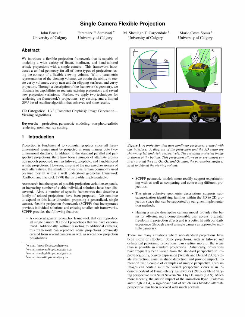
Figure 1: A projection that uses nonlinear projectors created withour interface. A diagram of the projection and the 3D setup areshown top left and right respectively. The resulting projected imageis shown at the bottom. This projection allows us to see almost en-tirely around the car. Q0, Q1, and Q2 mark the parametric surfacesused to defined the viewing volume.

• SCFPF geometric models more readily support experiment-ing with as well as comparing and contrasting different pro-jections.

• The given cohesive geometric descriptions supports sub-categorization identifying families within the 3D to 2D pro-jection space that can be supported by our given implementa-tion methods.

• Having a single descriptive camera model provides the ba-sis for offering more comprehensible user access to greaterfreedoms in projection effects and is a better fit with our dailyexperience (through use of a single camera as opposed to mul-tiple cameras).

There are many situations where non-standard projections havebeen useful or effective. Some projections, such as fish-eye andcylindrical panoramic projections, can capture more of the scenethan is possible in standard projections. Artistically, projectionshave frequently been varied from the standard perspective to im-prove legibility, convey expression [Willats and Durand 2005], cre-ate abstraction, assist in shape depiction, and provide impact. Tomention just a couple of examples of unique perspective, Cubismimages can contain multiple variant perspective views as in Pi-casso’s portrait of Daniel-Henry Kahnweller (1910), or blend vary-ing perspective as in Saint Severin No. 1 by Delaunay (1909). Muchmore recently, the artistic impact of the animation Ryan [Colemanand Singh 2004], a significant part of which uses blended alternateperspective, has been received with much acclaim.

Although clearly desirable for expanding the capabilities of graphicexpression, these non-standard projections are seldom seen in com-puter generated images. At least in part, this absence may be be-cause non-standard projections tend to be difficult to integrate intothe traditional graphics pipeline. The reason for this difficulty isthat unlike the standard projections, non-standard projections areoften nonlinear in nature and, consequently, are not representableas linear transformations in projection space. When this is thecase we categorize it as a nonlinear projection as suggested by Sa-lomon [2006]. Another reason for non-standard projections’ lack ofrepresentation in computer graphics is that previously no commonframework existed that was capable of creating all of these differentprojections. Non-standard projection implementations still tend tobe individually hand-tailored. This not only makes it time consum-ing and expensive to experiment with alternative projections, butmakes it nearly impossible for people not familiar with the neces-sary mathematical background.

Our framework introduces a unified geometry for a wide varietyof projections including linear, nonlinear, and artistic projections.This unification makes modeling and rendering of projections eas-ier and assists conceptually in understanding the interplay betweenthe scene, the projection, and the resulting image. Additionally, oursystem is underlaid by a relatively simple mathematical foundationand does not rely on compositing of individual projections into asingle image. In addition to introducing SCFPF, we discuss our im-plementation choices, including two rendering algorithms: one isbased on ray casting; the other uses scanline rendering to achieverealtime performance for a subset of our framework’s possible pro-jections.

In the next section, we review a variety of projection techniquesthat have been proposed in computer graphics. Section 3 definesand describes our framework. Section 4 provides the details of ourimplementation choices and of rendering SCFPF projections. InSection 5, we show results and discuss how projections from exist-ing works can be reproduced with SCFPF. Lastly, Section 6 presentsour conclusions and directions for future work.

2 Related Work

2.1 Single Camera Projections

Wyvill and McNaughton [1990] present Optical Models, a tech-nique for creating projections by mapping an image plane, ℜ2, toa set of rays originating from an image surface, ℜ5 (three coordi-nates and two angles). The definition of the mapping is left to theimplementation. This technique is capable of reproducing typicalcamera based projections, such as fish-eye projection, as well ashandling curved image planes. Similarly, Glassner [2000; 2004]creates cubist style projections. Like Optical Models, this systemis also suited to ray tracing; however, in this system the rays aredefined by two NURBS surfaces.

Levene’s non-realistic projections [1998] extends Inakage’s [1991]non-linear perspective projections and provides the capability tocreate a variety of artistic projections. This framework uses severalparameterized functions that allow users to control the shape of theprojection surfaces and the shape of convergence and divergence oforthogonals.

Kolb et al. [1995] developed a technique of reproducing assortedphotographic projections by physically simulating lens and camerabehaviors. These lens techniques rely on simulating light and con-sequently use a ray tracing approach.

Most recently, Wang et al. [Wang et al. 2005] presented a volumelens technique using ray casting. The rays are refracted at the image

plane based on the specific type of lens selected. A GPU pixelshader then steps through the 3D texture compositing a fragmentcolor based on texels encountered along the ray.

The General Linear Camera (GLC) model described by Yu andMcMillan [2004b] is able to reproduce a wide variety of linear pro-jections including perspective, orthogonal, push-broom [Gupta andHartley 1997], and crossed-slits [Zomet et al. 2003] projections.GLCs are described by three rays. Affine combinations of thesedefining rays are used to create the rays that sample the scene.

Salomon’s book on projections [2006] provides mathematicalderivations of a wide variety of linear and nonlinear projections.Wood et al. [1997] and Rademacher and Bishop [1998] have devel-oped systems of creating images that combine more than one view-point with a single camera. In Wood et al.’s work, camera paths areused to create a single panoramic image where local areas of the im-age have the appearance of a perspective projection. Rademacherand Bishop’s multiple-center-of-projection images can be describedas the result of moving a slit camera along a path through a scene.Mei et al. [2005] introduced the occlusion camera. The projectionproduced by this camera reveals occluded areas of a 3D objects toassist in image based rendering.

It is important to note that none of these single camera systems iscapable of reproducing all of the other single camera systems. InSection 5 we will discuss and demonstrate how these techniquescan be created within our framework.

2.2 Composite Projections

There is a rapidly growing body of work that deals with imagescreated by blending the results of two or more cameras’ projectionstogether. We refer to these projections as composite projections.Works that make use of composite projections include Agrawala etal. [2000], Singh [2002], and Coleman and Singh [2004]. Addition-ally Popescu et al.’s sampled-based cameras for rendering reflec-tions by blending together many linear camera’s projections can beviewed as producing a type of composite projection [2006]. Lev-ene’s non-realistic projections [1998], previously mentioned, alsoincludes support for simple composite projections. In general thesetechniques use multiple cameras positioned throughout the scene.These cameras produce images using linear projections (usuallyperspective or orthographic) and the main effort of these works liesin blending the images together to produce a coherent compositeimage as a result. This involves control of the blending process,possibly setting culling distance to keep far-away objects from de-forming into the scene, and imposing constraints to maintain geom-etry.

Singh and Balakrishanan [2004] introduce a projection where localareas of magnification are created by deforming the scene with aFFD deformation lattice. The deformed geometry is then projectedto an image.

A variation of composite projection is shown in works by Agarwalaet al. [2006], Collomosse and Hall [2003], and Claus and Fitzgib-bon [2005]. In these systems, photographs from cameras with un-registered positions and orientations are blended together to create:long images with a variety of vanishing points; non-photorealisticrendering of cubist style paintings; and remove radial distortion,respectively.

Another particular type of composite projection is encompassedby Yu and McMillan’s Framework for Multiperspective Rendering[2004a]. In this work the final image is created from a patchworkof tiles; each tile created by a different GLC. By controlling thetypes and parameters of cameras whose tiles neighbor one anotherC0 continuity in the resulting image is guaranteed.

In our system, we have chosen to concentrate on creating projec-tions with a single camera. This avoids the difficult process ofblending images together. It also yields an easily visualizable view-ing volume that assists in understanding the projection and fits wellinto our daily experience. Despite using a single camera our frame-work can reproduce some composite projection effects by bendingor splitting the image plane as is shown in Section 5.

3 Projection Framework

The current techniques for specifying projections in computergraphics involve deriving unique matrices from the type of projec-tion (i.e., parallel or perspective) and the camera specification (i.e.,viewing angle, position of clipping planes, etc).

We propose a new technique for specifying projections in which theuser models the geometry of the viewing volume. One can think ofour framework’s camera as starting with an orthogonal projection’sviewing volume (Figure 2) made from an elastic material. Thisviewing volume can then be deformed and manipulated to createthe desired volume and projection (Figure 3). The end result canbe a curvy volume, with curvy near and far clipping surfaces andcurvy projectors. Projectors are defined as curves (or lines) startingat the image plane (or image surface) and ending at the far plane(or surface), passing through all points in the scene that could beprojected onto the projector’s starting position.

Qn

fQdepth

Figure 2: Viewing volume of an orthogonal projection. We canimagine this as the starting point for SCFPF viewing volumes thatcan be deformed into various shapes. As will be standard through-out, projectors are shown as blue lines while surfaces within theviewing volume are green. Qn and Q f label the near and far planesof the volume.

Image

Re-parameterization

Projection Geometry

QQf

n

Figure 3: A complex projection’s geometry with nonlinear projec-tors. Re-parameterization provides a map between Qn and an im-age.

To accomplish this curvy result, we represent a projection’s viewingvolume as a parametric volume:

Q(u,v, t) =

x(u,v, t)y(u,v, t)z(u,v, t)

,u0 ≤ u ≤ u1v0 ≤ v ≤ v10 ≤ t ≤ 1

.

The parameter t corresponds to depth within the projection’s view-

ing volume while u and v identify position within the remainingdimensions (and eventually also the position in the resulting im-age).

To illustrate Q(u,v, t) let us begin with the orthographic projec-tion shown in Figure 2 and abstract it to a more general setting.For orthogonal projections, the viewing volume is a rectangularprism. From this volume, we can extract two important paramet-ric surfaces, the near plane, Qn = Q(u,v,0), and the far plane,Q f = Q(u,v,1). These planes become generalized as surfaces andare parameterized by u and v. Projectors within the orthogonalviewing volume become parallel lines that run between and are or-thogonal to the near and far planes. If given an arbitrary point pwithin this volume, we determine its projection by identifying theu,v coordinates of the projector that intersects p.

Each projector pu,v(t) = Q(u,v, t) within the volume originates atQn(u,v) and ends at Q f (u,v). When creating camera-like projec-tions (e.g., perspective, orthogonal, fish-eye) projectors are linear,composed of rays defined by the two points: Qn(u,v) and Q f (u,v).We discuss linear projections further in Section 3.2. To allow fullcontrol over all three dimensions of our parameterization, we alsoallow for nonlinear projectors. That is, projectors that follow acurved path through the 3D scene. The reasons for and effects ofallowing this freedom are further discussed in Subsection 3.3. Fig-ure 3 shows an example of a viewing volume with these nonlinearprojectors.

One remaining issue is that after we have deformed the viewingvolume, our surfaces Qn and Q f may no longer be planar. Con-sequently we may no longer have a concrete viewing plane withinthe volume. In these cases we use an extra step, that we call re-parameterization, to map projected points from Qn(u,v) to a view-ing plane (see Figure 3). Re-parameterization is described in Sub-section 3.4.

To render a given point p = (x,y,z) within the viewing volume wecalculate its parametric representation (u,v, t). To accomplish this,we identify the u,v coordinates of the projector that intersects pand then determine its depth along the projector. This step can beexpensive in the general case, however there are important casesthat lead to simple computations; we will discuss this in Section 4.

In Figure 4, we introduce a diagrammatic representation of theviewing volume. In these diagrams, we present orthogonal viewsof the viewing volume with attention to the key surfaces, Qn andQ f , that can be used to identify the characteristics and behavior ofthe projection. In addition, represented as blue lines, are a sam-pling of the viewing volume’s projectors. By following the projec-tors through the volume we can identify where points in the scenewill be projected in the image. The surfaces in these diagrams areshown in green and the projectors in blue. Additionally, we willshow the camera setup in perspective 3D when we wish to ensurethat the original shape of the models is understood and to assist indescribing some projections that are not easily described with anorthographic projection (such as the projection shown in Figure 7).

3.1 Relation to Volume Deformation

At this point, our parameterization of the camera’s viewing volumemight be seen as merely an extension of volume representation ordeformation such as free-form deformation (FFD) [Sederberg andParry 1986] or extended free-form deformation (EFFD) [Coquillart1990]. To show otherwise we ask you to consider an analogy: thegeometry of a pyramid was understood long before it was appliedto create the perspective viewing system in traditional art. This de-velopment, first scientifically analyzed during the Renaissance con-stituted a breakthrough for viewing systems. With this in mind, our

zy

n

f

Q

Q

zy

fn QQ

zy

nf

QQ

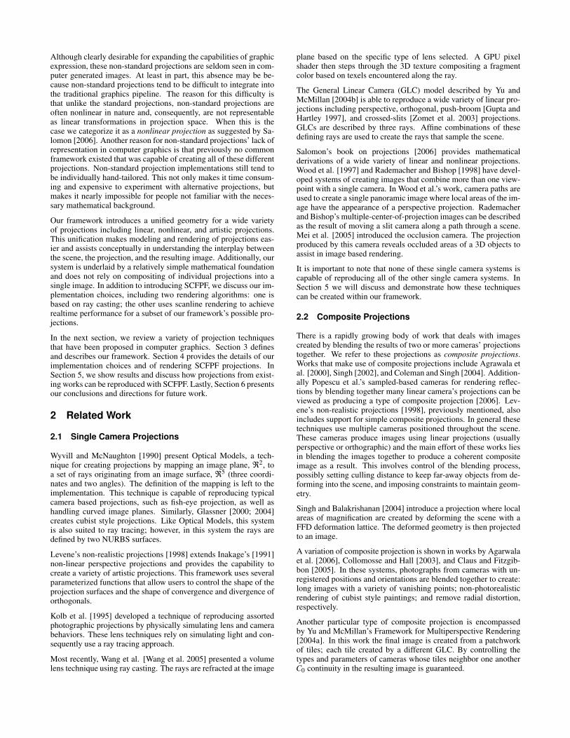
Figure 4: Creating perspective (left), orthogonal (center), and in-verted perspective projections (right). The diagram of the setup ofeach projection is shown on the left while resulting image is shownon the right.

goal has been to present the idea of accomplishing projection bydeforming the viewing volume. Notice that our goal is not to ob-tain (or see) deformed objects in the scene; rather it is to observewhat happens to the objects after projection (in a nonlinear fashion)to a 2D surface. This creates a variety of new possibilities for cre-ating projections. It is also worthwhile to note that these volumedeformation techniques begin with a regular volume, determine the3D parameterization of objects, and then find the objects’ locationin the deformed volume. SCFPF is the dual, with the reverse taskof determining the objects’ parameterization in the deformed vol-ume so the object can be shown within a regular volume (i.e., theviewbox).

3.2 Projection with Linear Projectors

When dealing with linear projectors it is possible to define the entirevolume by specifying the two parametric surfaces Qn and Q f . It isimportant to note that these surfaces need not be rectangles or evenplanes. The volume between these surfaces becomes the viewingvolume of the projection. We represent this parametrically as:

Q(u,v, t) = (1− t)Qn(u,v)+ tQ f (u,v)

t ∈ [0,1], u ∈ [u0,u1], v ∈ [v0,v1]where u0,u1,v0, and v1 represent the lower and upper bounds of theparameters used for Qn and Q f .

We construct projectors leading from Qn to Q f . The definition ofthe projector that originates at Qn(u0,v0) becomes:

qu0,v0(t) = (1− t)Qn(u0,v0)+ tQ f (u0,v0) t ∈ [0,1].

Points on a particular projector that are at a depth (t) greater thanone or less than zero are not included in the image. This provides afar and near clipping distance for each projector.

Now we will show that a perspective projection created by ourframework is indeed the perspective projection we are familiar within computer graphics. In Figure 4 we created the perspective pro-jection using two square patches with normals parallel to the z-axis.Our surface Qn is a small square and our surface Q f is a largersquare. The center of each square is aligned. These parametricsquares are defined as: x

yz

=

cx + lucy + lvcz

where c = (cx,cy,cz) is the center of the square and l is half thewidth of the square. In our projection we set cn = (0,0,1) andc f = (0,0,2), ln = 1, and l f = 2. With Qn and Q f defined, ourviewing volume is:

Q(u,v, t) = (1− t)[cn +(1,0,0)u+(0,1,0)v]+

t[c f +(2,0,0)u+(0,2,0)v].

From this we get: xyz

=

(1− t)u+2tu(1− t)v+2tv(1− t)+2t

.

We solve for p∗ = (u,v, t) and find: uvt

=

xzyzz−1

.

Let us now look at how we can produce some common projec-tions. By using two square, parallel planes it is simple to reproduceperspective, orthogonal, and inverse perspective projections as isshown in Figure 4. Let us examine our definition of a perspectiveprojection within SCFPF a little more closely. Our surface Qn isa small parametric rectangle while Q f is a larger rectangle. In theperspective projection shown in Figure 4 the center of each rectan-gle is aligned, although this is not always necessary. However, tocreate a perspective projection, the ratios of width to height of thesetwo rectangles must be the same and the surfaces must be parallelto one another. This ensures that the projectors converge to a sin-gle viewing point. By varying the sizes of Qn and Q f , as well astheir centers, while ensuring that the projectors converge to a singlepoint, we can recreate all possible perspective projections.

It is worth noticing that by shifting Qn or Q f and changing theirwidth to height ratios in ways to cause the projectors to no longerconverge, we can create entirely new, but somehow related projec-tions. In Figure 5, we present an irregular perspective projectionthat removes the distortion that is created in the columns perpen-dicular to the near plane in a wide angle perspective projection.This brief example begins to convey the flexibility and power ofour framework’s ability to create, modify, and explore the space ofpossible projections.

One last, pertinent point is in our linear perspective projection,depth of a point in the viewbox, p = (x,y,z), parameterized as(u,v, t) is t. Parameter t can be calculated as t = p−Qn(u,v)

Q f (u,v)−Qn(u,v) .This is contrary to most 3D graphics applications [Watt 2000]where linear perspective projection’s depth is calculated as:t̄ = f−d/z

f−d where f , d, and z are the distances from the center ofprojection (COP) to the far plane, near plane, and p respectively.This difference can be corrected with a re-parameterization of thedepth coordinate t to linear perspective depth t̄.

Nonlinear Projections

It is also possible to use linear projectors to create nonlinear projec-tions by creating viewing volumes where Qn or Q f are curvy sur-faces. For example, by using a small circle (or small hemisphere)as Qn and a hemisphere centered at that point as Q f we achievean angular fish-eye projection [Salomon 2006] (Figure 8). Anotherpopular nonlinear projection is the cylindrical panoramic projec-tion. This is formed by placing one cylinder, Qn, within anotherlarger cylinder, Q f (Figure 6).

zx

nQ

fQ

nQ

Figure 6: A cylindrical panorama projection can be created with two nested cylinders.

zy

nf QQ

zx

nf QQ

zx

nf QQ

Figure 5: Comparison between perspective and irregular perspec-tive projections. From left to right the top row of diagrams presentthe side view of both projections, the top view of perspective, andthe top view of irregular perspective. In the middle and bottom rowswe present the 3D volume and the results of perspective (left) andirregular perspective (right) projections respectively. Notice thatthe odd looking distortion of the columns in the perspective resultis almost entirely absent in the irregular perspective result.

The major advantage of this geometric technique for composingprojections is that it becomes much easier to visualize, create, andadjust created projections. Rather than dealing with the underly-ing math, parameters in equations, projections are created throughmanipulating these relatively simple surfaces and projectors.

3.3 Nonlinear Projectors

By allowing projectors to assume curvy paths between Qn and Q f ,we can greatly increase the diversity of projections made possibleby our framework. Nonlinear projectors allow the nature of theprojection to be changed, based on the depth within the viewingvolume. The nonlinear projectors are parametric curves, qu0,v0(t)for any fixed (u0,v0).

In Figure 7, we show an example of the difference in control overthe projection made possible by using nonlinear projectors. Nonlin-ear projectors not only allow more control over the position wherea projector intersects an object, but also provide control over theangle at which the projector intersects the object. This is importantin creating complicated projections such as those in Figures 11 and13.

nQ

fQ

nQ

fQ

Figure 7: Comparison of a linear twist projection (left) to a non-linear projection (right).

3.4 Re-parameterization

With the viewing volume Q(u,v, t) and a given point in the scenep = (x,y,z) we calculate the projection by finding p’s parameteriza-tion, p = (u,v, t). Once we have projected all the points, we need tomap (u,v, t) to an image. We call this operation re-parameterization.This operation can be visualized as mapping Qn(u,v) to a viewingsurface (screen). Most often this viewing surface will be a plane,but for special applications other surfaces may prove useful. Forexample, if we had a curved monitor, we could map to the moni-tor’s particular curved shape. When Qn(u,v) is a parametric surfacepatch, the re-parameterization is as easy as interpreting (u,v) as thewidth and height specifications of pixels in the image. However, ifwe happen to use parametric surfaces based on polar coordinates(e.g., a circle, sphere, or hemisphere) a map from polar coordinatesto a rectangular shape in Cartesian coordinates is necessary.

Aside from achieving a flat, rectangular image, re-parameterizationcan be used to produce other useful effects by resampling the pa-rameterization. A wide variety of possible distortions exist; suchdistortions can be taken from practically any image space distor-tion technique such as magic lenses [Yang et al. 2005], or distor-tion viewing [Carpendale and Montagnese 2001]. One possibilityis magnifying a specific local area of the image to produce a mag-nifying lens effect. Another would be in creating a global distortionthat changes an angular fish-eye projection into a lens-like fish-eye.In this distortion, shown in Figure 8, objects nearest the center ofthe circle appear larger while objects further from the center be-come compressed.

4 Implementation and Interface

When previously discussing nonlinear projectors, we have left themethod for specifying the shape of these curves open. In this sec-

zy

n

f

QQ

n

f

Q

Q

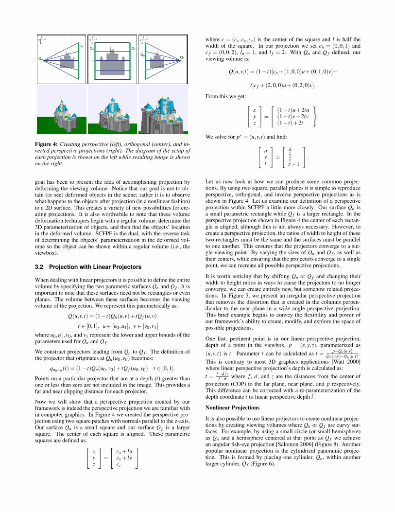
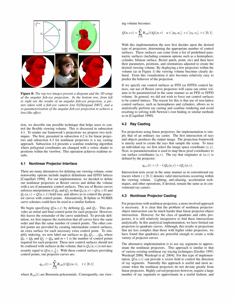
Figure 8: The top two images present a diagram and the 3D setupof the angular fish-eye projection. In the bottom row, from leftto right are the results of an angular fish-eye projection, a pic-ture taken with a fish-eye camera lens ©[Dargaud 2007], and are-parameterization of the angular fish-eye projection to achieve alens-like effect.

tion, we describe one possible technique that helps users to con-trol the flexible viewing volume. This is discussed in subsection4.1. To render our framework’s projections we propose two tech-niques. The first, presented in subsection 4.2 is for linear projec-tors and subsection 4.3 for nonlinear projectors is a ray castingapproach. Subsection 4.4 presents a scanline rendering algorithmwhere polygonal coordinates are changed with a vertex shader topositions within the viewbox. This operation achieves realtime re-sults.

4.1 Nonlinear Projector Interface

There are many alternatives for defining our viewing volume, somenoteworthy options include implicit definitions and EFFD lattices[Coquillart 1990]. For our implementation, we decided to defineour nonlinear projectors as Bezier curves and define the volumewith a set of parametric control surfaces. This use of Bezier curvesenforces interpolation of Qn and Q f so that Qn(u,v) = Q(u,v,0) andQ f (u,v) = Q(u,v,1) hold true, and allows us to control the projec-tor curves with control points. Alternatively, B-Spline or NURBScurve schemes could have be used in a similar fashion.

We begin specifying Q(u,v, t) by defining Qn and Q f . This pro-vides an initial and final control point for each projector. However,this leaves the remainder of the curve undefined. To provide defi-nition, we first impose the restriction that all curves have the sameorder and thus the same number of control points. The other con-trol points are provided by creating intermediate control surfaces,an extra surface for each necessary extra control point. To sim-plify indexing, we now label our surfaces as Q0,Q1, ...,Qm whereQn = Q0 and Q f = Qm and m + 1 is the number of control pointsrequired for each projector. These new control surfaces should notbe confused with surfaces in the volume; that is Q1(u,v) is not nec-essarily equal to Q(u,v, 1

m ). With these control surfaces providingcontrol points, our projector curves are:

qu,v(t) =m

∑i=0

Bi,m(t)Qi(u,v), t ∈ [0,1]

where Bi,m(t) are Bernstein polynomials. Consequently, our view-

ing volume becomes:

Q(u,v, t) =m

∑i=0

Bi,m(t)Qi(u,v) u ∈ [u0,u1], v ∈ [v0,v1], t ∈ [0,1].

With this implementation the user first decides upon the desiredtype of projectors, determining the appropriate number of controlsurfaces. These surfaces can come from a list of predefined para-metric surfaces (including common options such as a hemisphere,cylinder, bilinear surface, Bezier patch, point, etc) and then havetheir parameters, positions, and orientations adjusted to create thedesired viewing volume. By displaying a few projectors within thevolume (as in Figure 1) the viewing volume becomes clearly de-fined. From this visualization it also becomes relatively easy topredict the behavior of the projection.

If we specify our control surfaces as FFD (or EFFD) control lat-tices, our use of Bezier curve projectors will cause our entire vol-ume to be parameterized in the same manner as an FFD or EFFDvolume. In general, we did not wish to force our control surfacesto be control lattices. The reason for this is that use of non-latticecontrol surfaces, such as hemispheres and cylinders, allows us toanalytically perform ray casting and scanline rendering and avoidresorting to solving with Newton’s root finding or similar methodsas in [Coquillart 1990].

4.2 Ray Casting

For projections using linear projectors, the implementation is sim-ply that of an ordinary ray caster. The first intersection of raysand objects produces the output image. The projection frameworkis merely used to create the rays that sample the scene. To tracean individual ray, we first select the image space coordinate (x,y).Next, re-parameterization is used to map these pixel coordinates toour surface coordinates (u,v). The ray that originates at (u,v) isdefined by the projector:

qu,v(t) = (1− t)Qn(u,v)+ tQ f (u,v).

Intersection tests occur in the same manner as in conventional raytracers where t ∈ [0,1] denotes valid intersections occurring withinthe viewing volume. Lighting, anti-aliasing, acceleration tech-niques, and other operations, if desired, remain the same as in con-ventional ray casters.

4.3 Nonlinear Projector Casting

For projections with nonlinear projectors, a more involved approachis necessary. It is clear that the problem of nonlinear projector-object intersection can be much harder than linear projector-objectintersection. However, for the class of quadratic and cubic pro-jectors, it is still relatively inexpensive to find these intersectionsanalytically. In this analytical implementation, we have limited ourprojectors to quadratic curves. Although, this results in projectionsthat are less complex than those with higher order projectors, wehave found that quadratics are powerful enough to create a widevariety of projector curves.

The alternative implementation is to use ray segments to approx-imate the nonlinear projectors. This approach is similar to thatof various existing nonlinear ray tracing techniques [Groller 1995;Weiskopf 2000; Weiskopf et al. 2004]. For this type of implemen-tation, Q(u,v, t) can provide a vector field to control the directionof ray segments. Naturally this approach is useful and most ac-curate when the nonlinear projectors do not deviate greatly fromlinear projectors. Highly curved projectors however, require a largenumber of ray segments to approximate in a useful fashion, and

consequently may require higher computational costs to achieve ac-curacy.

A difference between our nonlinear projector casting and ray cast-ing is the question of how to deal with specular highlights whenperforming Phong lighting calculations. Specular highlights are de-termined by (R ·V )n where V is the direction to the viewer, R is thelight reflection vector, and n denotes the specular power. The prob-lematic term here is V . In our projections, we do not necessarilyhave a view location or a straight projector (as is the case in Figure1) to provide this term. Our approach is to use an estimate of theprojector’s tangent at the point of intersection. This is a reasonableapproach as it takes into account the path of the projector at thepoint in space where it intersects the object.

4.4 Scanline Rendering Algorithm

Our scanline rendering algorithm makes use of the renderingpipeline to produce realtime SCFPF projections. In its current state,this algorithm is only capable of rendering a subset of the projec-tions within our framework.

In this algorithm, we render scenes through our projections with thehelp of vertex shaders. We use vertex shaders to move vertices fromtheir position in the original geometry to their projected position inthe viewbox. Then the existing hardware scanline rendering systemrenders the triangles of the model. This algorithm is extremely fastalthough the scanline rendering of triangles can result in inaccura-cies in rendering and clipping when coarse models are used. Thisis due to projection of vertices, rather than all points of each trian-gle. This problem can be alleviated by subdividing the models inthe scene.

The primary task of our scanline algorithm is, for each vertex of thescene, to change its spatial representation (x,y,z) to a parametricrepresentation (u,v, t). Re-parameterization requires an additionalstep where the u and v values are changed based on the specifiedre-parameterization mapping.

To solve for (u,v, t), let us start by assuming that for a givenp = (x,y,z), t = t ′ is known where t ′ is the particular depth valueof the vertex within the projection volume (we describe how t ′ iscalculated shortly). The step here is to solve for u and v. Hav-ing the description of the volume Q(u,v, t), we are able to find theiso-surface Q′

t(u,v) = Q(u,v, t ′) that p is located on. Next we forthe u and v coordinates for p on Qt ′(u,v). The exact details of thissolution depends on the definition of Qt ′(u,v).

As we are solving for two unknowns (u and v) with three knownequations (the parametric equations for x, y, and z that defineQt ′(u,v)) this algorithm is generally limited to projection geome-try where Qt ′(u,v) can be defined by first degree equations. Oncewe have solved for u and v, we then perform the re-parameterizationmapping on (u,v).

To complete the calculation of (u,v, t) from (x,y,z), we need to findt = t ′. Therefore, the parameter t must be calculable with knowl-edge of Q(u,v, t) and p. Simple examples of where this is possi-ble are the linear projections shown in Figure 4. For these projec-tions, t can be calculated by the ratio of the distance of p to Qn tothe distance between Qn and Q f . Other projections for which thisalgorithm can be used, have all of their u,v iso-surfaces (that is,Qt(u,v)) parallel to one another. We can further extend this to pro-jections with parametric surfaces that are equally distant from oneanother at all points (i.e., as in the case of nested spheres or cylin-ders). Examples of possible projections include projections withnonlinear projectors like those in Figures 7 and 9. Figure 1 pro-vides an example of a projection where estimating t is not possibleand thus cannot implemented with our scanline technique. Another

example of a situation where scanline rendering is not possible isprojections where a point (x,y,z) can be mapped to more than one(u,v, t) coordinate.

Our description to this point has been applied to our single cameraflexible projection framework in general; however with our spe-cific implementation (using control surfaces) there are some ad-ditional considerations. Firstly, if the control surfaces are all thesame type of parametric surface, then Qt ′(u,v) is easily extractedfrom Q(u,v, t) as a surface of this same type. The second consider-ation is that since vertex shaders cannot be overly complex, due tohardware considerations, each type of parametric surface requires adifferent vertex shader to be implemented to solve for (u,v) givenp on the surface.

5 Reproducing Various Projections

Now that we have presented our framework and its implementationwe discuss how a variety of projections can be reproduced. We re-produce these projections by discussing how to recreate the geome-try of the projections. In some cases additional re-parameterizationmay be necessary to achieve accurate depth values in the projectedcoordinates.

When working with linear projectors and without re-parameterization, our framework behaves in the same manner asOptical Models [1990]. Similarly we can reproduce Glassner’sDigital Cubism [2000; 2004] by defining our viewing volumethrough NURBS surfaces. Figures 4, 6, and 8 demonstrate projec-tions that are commonly reproducible by Optical Models, DigitalCubism, and SCFPF. Our technique introduces improvement overthese related techniques in three areas. The first is that we introducenonlinear projectors. These projectors allow the projection tochange its characteristics through the depth of the viewing volume.The second is the re-parameterization step that allows the resultingimage to be resampled as desired. For example, in Figure 8 itallows us to resample our angular fish-eye to better resemblethe photographic fish-eye image. Lastly our technique features ascanline algorithm (albeit a limited one).

As opposed to Kolb et al.’s physical simulation [1995], our goalis not to reproduce all the physical effects present in the camerasuch as focus, chromatic aberration, etc; but instead to provide aunified method of creating projections. We have shown that wecan approximately reproduce a camera’s fish-eye projection (Figure8). Other lens simulations are reproducible with linear projectorsthat collect the scene’s light onto a surface representing the shapeof the lens and an appropriate mapping function applied for re-parameterization that mimics the lens’ reorganization of light ontothe film surface.

In Magic Volumes [Wang et al. 2005] three different projectionsusing linear projectors are described. The first, called the magnifi-cation lens, changes the direction of a subset rays to point toward asingle point on the far plane, instead of being directed orthogonally.This single point is surrounded by a transition region where the raydirection is pointed slightly toward this single, magnification point.With SCFPF this effect can be produced by using a linear, planar,B-Spline patch with a fine resolution of control points. The magni-fication point can be created by collapsing several neighboring con-trol points to a single position and by moving surrounding controlpoints closer to this location. The second projection, the sample-rate-based lens, is produced by changing the sampling of the im-age plane to produce areas of magnification. This is easily accom-plished with SCFPF by using an appropriate re-parameterizationmapping. Lastly, we have already shown production of the fish-eyelenses that are the third projection presented for Magic Volumes.

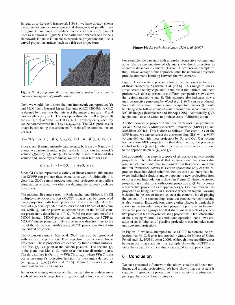
In regards to Levene’s framework [1998], we have already shownthe ability to control convergence and divergence of parallel linesin Figure 4. We can also produce curved convergence of parallellines as is shown in Figure 9. One particular drawback of Levene’sframework is that it is unable to reproduce projections that use acurved projection surface (such as a fish-eye projection).

zx

02 QQ

1Q

Figure 9: A projection that uses nonlinear projectors to createcurved convergence of parallel lines.

Next, we would like to show that our framework can reproduce Yuand McMillan’s General Linear Cameras (GLC) [2004b]. A GLCis defined by three rays that intersect the image plane at z = 0 andanother plane at z = 1. The rays pass through z = 0 at (ui,vi,0)for i = [1,2,3] and the z = 1 at (si, ti,1). Consequently, each raycan be parameterized in 4D by (si, ti,ui,vi). The GLC produces animage by collecting measurements from the affine combinations ofthe rays:

r = α(s1, t1,u1,v1)+β (s2, t2,u2,v2)+(1−α −β )(s3, t3,u3,v3).

Since α and β simultaneously parameterize both the z = 0 and z = 1planes, we can use α and β as the u and v terms per our framework’svolume Q(u,v, t). Qn and Q f become the planes that bound thisvolume and, since rays are linear, we use a linear term for t as:

Q(u,v, t) = (1− t)Qn(u,v)+ tQ f (u,v).

Since GLCs can reproduce a variety of linear cameras, this meansthat SCFPF can produce these cameras as well. Additionally it isclear that GLCs cannot produce nonlinear projectors as any affinecombination of linear rays (the rays defining the camera) produceslinear rays.

The moving slit camera used in Rademacher and Bishop’s [1998]multiple-center-of-projection (MCOP) images can be reproducedusing projection with linear projectors. The surface Qn takes theform of a general cylinder that follows the MCOP path of the cam-era, while Q f can be piecewise defined based on the MCOP cam-era parameters, described as (Ci,Oi,Ui,Vi) for each column of theMCOP image. MCOP projections cannot produce our SCFP asMCOPs’ image plane can only curve in one direction due to theuse of the slit camera. Additionally MCOP projections do not uti-lize curved projectors.

The occlusion camera [Mei et al. 2005] can also be reproducedwith our flexible projection. This projection uses piecewise linearprojectors. These projectors are defined by three control surfaces.The first, Q0 is a point at the camera position. The second, Q1is the plane that Mei et al. refer to as the near distortion plane.The third surface is Q3(u,v) = PPHC((u,v,z f ) where PPHC is theocclusion camera’s projection function for the camera defined by(u0,v0,zn,z f ,dn,d f ) [Mei et al. 2005]. Figure 10 shows a visual-ization of an occlusion camera.

In our experiments, we observed that we can also reproduce somekinds of composite projections using our single camera projections.

Figure 10: An occlusion camera [Mei et al. 2005].

For example, we can start with a regular perspective volume, andadjust the parameterization of Q1 and Q2 to direct projectors toapproximate separate cameras (Figure 11 presents an example ofthis). The advantage of this approach is that the nonlinear projectorsprovide automatic blending between the two cameras.

Figure 11 was create to produce a long street panorama in the spiritof those created by Agarwala et al. [2006]. This image follows astreet across the cityscape and, in the result that utilizes nonlinearprojectors, is able to present two different perspective views downthe regions marked A and B. This example also indicates how amultiperspective panorama by Wood et al. [1997] can be produced.To create even more dramatic multiperspective images Qn couldbe changed to follow a curved route through the scene much likeMCOP images [Radmacher and Bishop 1998]. Additionally Q f ’sheight could also be varied to produce areas of differing zoom.

Another composite projection that our framework can produce isYu and McMillan’s Multiperspective Framework (MPF) [Yu andMcMillan 2004a]. This is done as follows. For each tile i of theMPF image, we can construct the corresponding GLC with a SCFPvolume defined with linear projectors by Qni and Q fi . Our volumefor the entire MPF projection is then described by the piecewisecontrol surfaces Qn and Q f where each piece of surfaces correspondto the appropriate piece Qni and Q fi .

Let us consider that there is a space of all possible non-compositeprojections. The related work that we have mentioned covers dis-joint subsets and individual solutions within this space. We arguethat our framework covers this entire space; not only can we re-produce these individual solutions; but, we can also interpolate be-tween individual solutions and extrapolate to new projections fromexisting ones. Interpolation is shown in Figure 12 where the createdprojection is similar to an orthogonal projection at Q0 but becomesa perspective projection as it approaches Q2. One can imagine thisprojection as being useful in a scenario where orthogonal viewingis desired in the area of focus (i.e., near the camera), but displayingthe context of the surrounding scene via perspective depth cueingis also wanted. Extrapolation, among other places, is particularlyshown in the irregular perspective projection portrayed in Figure 5where we produce a projection that shares many aspects of perspec-tive projection but is beyond existing projections. Our deformationof the viewing volume is a continuous operation that allows cre-ation of an infinite set of possible projections that includes manyundiscovered projections.

In Figure 13, we have attempted to use SCFPF to recreate the pro-jection that M. C. Escher has created in Study for House of Stairs,Pencil and Ink, 1951 [Locker 2000]. Although there are differencesbetween our image and his, this example shows that SCFPF pro-vides the capability of recreating customized artistic projections.

6 Conclusion

We have presented a framework that allows creation of linear, non-linear, and artistic projections. We have shown that our system iscapable of reproducing projections from a variety of existing com-puter graphics projection techniques.

nQ

fQ

nQ

fQ

Figure 11: Effects of nonlinear projectors. At the top we showthe construction of two projections, one with linear projectors (left)the other with nonlinear projectors (right). The resulting imagesproduced by these projections are shown in the middle and bottomimages. The nonlinear projectors have been used to create perspec-tive viewpoints in areas A and B. Orange ellipses mark the areas ofchange.

zy

20 QQ 1Q1Q

0Q

2Q

Figure 12: A projection with nonlinear projectors that is a blend ofan orthogonal and a perspective projection.

We have also introduced nonlinear projectors. While nonlinear pro-jectors have been used in other works, our control of the projectorsis the first to not require ray integration (in contrast to nonlinear raytracing by Groller [1995] and Weiskopf et al. [2004]). Nonlinearprojectors are a key element of allowing control over where and atwhat angle projectors intersect objects.

The most important aspect of this framework is that it allows usersto create projections in a geometric and unified fashion. This geo-metric modeling of projections draws on previous computer model-ing experiences and avoids tricky, mathematical, hand-tailored pro-jections. The unified aspect of this system enables us to conceptu-alize and use a variety of projections in the same way. It is thereforeeasier to compare and contrast projections with one another.

Lastly, we have described two different rendering implementations:one that makes use of graphics hardware to achieve real time per-formance, the other based on ray casting.

zy

n

f

Q

Q

zy

n

f

QQ

fQ

nQ

fQ

nQ

Figure 13: Recreating the projection used in Study for House ofStairs, Pencil and Ink, 1951 by M. C. Escher [Locker 2000] usingSCFPF. On the left we show the details of the setup and result of aperspective projection. On the right we present our designed imita-tion projection.

6.1 Limitations and Future Work

A key limitation of our method lies in efficiency. Although we canreproduce a wide variety of projections, including some compositeprojections, the generality of the framework makes efficient pro-jection difficult. E.g., in MCOP images [Radmacher and Bishop1998] their composite viewing volume is produced by varying theparameters of strip camera as it follows a path through the scene.However, since a SCFPF control surface may have any shape (andsince projectors may be curved) we cannot simply change the para-meters of a linear camera across the image. Consequently we relyon ray casting, aside from special cases where scanline rendering ispossible.

Our current GPU implementation is limited; creating a less restric-tive interactive technique is a major goal in our future work. Thecasting algorithm also presents interesting challenges. One chal-lenge is adapting ray-based acceleration techniques, such as useof the spatial subdivision, to nonlinear projector intersection tests.Another idea to be addressed is in extending nonlinear projectorcasting to nonlinear projector tracing; handling of reflections andrefraction in a predictable and coherent manner is a key concern. Itis our intuition that the distortion of the view volume does not dis-tort the scene’s actual geometry and consequently reflections andrefractions should be calculated using rays, rather than nonlinearprojectors.

Another key area in future work is to examine useful interfaces forcreating these projections. Our experience has shown that an inter-face capable of taking a sketched user input of direction and angleof intersection to create the parameterized viewing volume wouldgreatly assist in creating projections with nonlinear projectors.

Lastly, there should be more work done to directly compare thecapabilities of SCFPF and composite projections. Although SCFPFis capable of creating some composite projections (see Figure 11) itis not clear to what extent the two techniques overlap one another.It is likely that the most complete projection system would employcomposition of SCFPF projections.

Acknowledgements

We are grateful to Katayoon Etemad for her modeling assistance, toRuth Hart-Budd and Mark Hancock for their assistance in editing,and the referees for insightful and helpful reviews. The supportof the Natural Sciences Research Council of Canada and iCore isappreciatively acknowledged.

References

AGARWALA, A., AGRAWALA, M., COHEN, M., SALESIN, D.,AND SZELISKI, R. 2006. Photographing long scenes with multi-viewpoint panoramas. ACM Transactions on Graphics 25, 3,853–861.

AGRAWALA, M., ZORIN, D., AND MUNZNER, T. 2000. Artisticmultiprojection rendering. In Proceedings of the EurographicsWorkshop on Rendering Techniques 2000, Springer-Verlag, 125–136.

CARLBOM, I., AND PACIOREK, J. 1978. Planar geometric pro-jections and viewing transformations. ACM Comput. Surv. 10, 4,465–502.

CARPENDALE, M. S. T., AND MONTAGNESE, C. 2001. A frame-work for unifying presentation space. In UIST ’01: Proceedingsof the 14th annual ACM symposium on User interface softwareand technology, ACM Press, 61–70.

CLAUS, D., AND FITZGIBBON, A. W. 2005. A rational func-tion lens distortion model for general cameras. In Proc. of the2005 IEEE Computer Society Conference on Computer Visionand Pattern Recognition (CVPR’05), IEEE Computer Society,vol. 1, 213–219.

COLEMAN, P., AND SINGH, K. 2004. Ryan: rendering your an-imation nonlinearly projected. In NPAR ’04: Proceedings ofthe 3rd international symposium on Non-photorealistic anima-tion and rendering, ACM Press, 129–156.

COLLOMOSSE, J. P., AND HALL, P. M. 2003. Cubist style render-ing from photographs. IEEE Transactions on Visualization andComputer Graphics 9, 4, 443–453.

COQUILLART, S. 1990. Extended free-form deformation: a culp-turing tool for 3d geometric modeling. Computer Graphics (Pro-ceedings of ACM SIGGRAPH 90) 24, 4, 187–196.

DARGAUD, G. 2007. Fisheye photography.http://www.gdargaud.net/Photo/Fisheye.html, January.

GLASSNER, A. S. 2000. Cubism and cameras: Free-form opticsfor computer graphics. Tech. Rep. MSR-TR-2000-05, Microsoft.

GLASSNER, A. S. 2004. Digital cubism. IEEE Computer Graphicsand Applications 24, 3 (May-Jun), 82–90.

GROLLER, E. 1995. Nonlinear ray tracing: Visualizing strangeworlds. The Visual Computer 11, 5 (May), 263–274.

GUPTA, R., AND HARTLEY, R. I. 1997. Linear pushbroom cam-eras. IEEE Trans. Pattern Anal. Mach. Intell. 19, 9, 963–975.

INAKAGE, M. 1991. Non-linear perspective projections. In Mod-eling in Computer Graphics (Proceedings of the IFIP WG 5.10),203–215.

KOLB, C., MITCHELL, D., AND HANRAHAN, P. 1995. A realisticcamera model for computer graphics. In Proceedings of ACMSIGGRAPH 95, ACM Press / ACM SIGGRAPH, 317–324.

LEVENE, J. 1998. A framework for non-realistic projections. Mas-ter’s thesis, Massachusetts Institute of Technology.

LOCKER, J. L. 2000. The Magic of M. C. Escher. Harry N. AbramsInc., New York.

MEI, C., POPESCU, V., AND SACKS, E. 2005. The occlusioncamera. Computer Graphics Forum 24, 3, 335–342.

POPESCU, V., SACKS, E., AND MEI, C. 2006. Sample-based cam-eras for feed forward reflection rendering. IEEE Transactions onVisualization and Computer Graphics 12, 6, 1590–1600.

RADMACHER, P., AND BISHOP, G. 1998. Multiple-center-of-projection images. In Proceedings of ACM SIGGRAPH 98,ACM Press / ACM SIGGRAPH, 199–206.

SALOMON, D. 2006. Transformations and Projections in Com-puter Graphics. Springer-Verlag.

SEDERBERG, T. W., AND PARRY, S. R. 1986. Free-form defor-mation of solid geometric models. In Computer Graphics (Pro-ceedings of ACM SIGGRAPH 86), 20, 4, ACM Press, 151–160.

SINGH, K., AND BALAKRISHNAN, R. 2004. Visualizing 3d scenesusing non-linear projections and data mining of previous cam-era movements. In AFRIGRAPH ’04: Proceedings of the 3rdinternational conference on Computer graphics, virtual reality,visualisation and interaction in Africa, ACM Press, 41–48.

SINGH, K. 2002. A fresh perspective. In Graphics Interface, 17–24.

WANG, L., ZHAO, Y., MUELLER, K., AND KAUFMAN, A. 2005.The magic volume lens: An interactive focus+context techniquefor volume rendering. VIS 00, 47.

WATT, A. 2000. 3D Computer Graphics, third ed. Addison-WesleyPublishing Company Inc.

WEISKOPF, D., SCHAFHITZEL, T., AND ERTL, T. 2004. Gpu-based nonlinear ray tracing. Computer Graphics Forum 23, 3,625–633.

WEISKOPF, D. 2000. Four-dimensional non-linear ray tracing as avisualization tool for gravitational physics. VIS 00, 12.

WILLATS, J., AND DURAND, F. 2005. Defining pictorial style:Lessons from linguistics and computer graphics. Axiomathes 15,319–351(33).

WOOD, D. N., FINKELSTEIN, A., HUGHES, J. F., THAYER,C. E., AND SALESIN, D. H. 1997. Multiperspective panora-mas for cel animation. In Proceedings of ACM SIGGRAPH 97,ACM Press / ACM SIGGRAPH, 243–250.

WYVILL, G., AND MCNAUGHTON, C. 1990. Optical mod-els. In Proceedings of the eighth international conference of theComputer Graphics Society on CG International ’90: computergraphics around the world, Springer-Verlag, 83–93.

YANG, Y., CHEN, J. X., AND BEHESHTI, M. 2005. Nonlinearperspective projections and magic lenses: 3d view deformation.IEEE Computer Graphics and Applications 25, 1, 76–84.

YU, J., AND MCMILLAN, L. 2004. A framework for multiper-spective rendering. In 15th Eurographics Symposium on Ren-dering (EGSR04), 61–68.

YU, J., AND MCMILLAN, L. 2004. General linear cameras. InComputer Vision - ECCV 2004, Springer Berlin / Heidelberg,vol. 2, 14–27.

ZOMET, A., FELDMAN, D., PELEG, S., AND WEINSHALL, D.2003. Mosaicing new views: The crossed-slits projection. IEEETransactions on Pattern Analysis and Machine Intelligence 25,6, 741–754.