Educational Attainment Effects of High School Curriculum Tracking in the United States Sinan Gemici National Centre for Vocational Education Research L11, 33 King William Street Adelaide, South Australia 5000 [email protected] This manuscript has been submitted to the International Journal of Vocational Education and Training

Welcome message from author
This document is posted to help you gain knowledge. Please leave a comment to let me know what you think about it! Share it to your friends and learn new things together.
Transcript
Educational Attainment Effects of High School Curriculum Tracking in the United States
Sinan Gemici National Centre for
Vocational Education Research L11, 33 King William Street
Adelaide, South Australia 5000 [email protected]
This manuscript has been submitted to the International Journal of Vocational Education and Training

EDUCATIONAL ATTAINMENT EFFECTS 1
Abstract
Decades of research on the outcomes of curriculum tracking in the United States have produced
inconsistent results, mainly due to insufficient attention to selection bias. Data from the National
Longitudinal Survey of Youth 1997 (NLSY97) were used to conduct a re-assessment of high
school tracking effects on educational attainment, with a particular focus on addressing bias from
non-random selection into curriculum tracks. Career-technical education and college-preparatory
tracks produced favorable outcomes at distinct attainment levels when compared to general
tracks. Results indicate a need to qualify blanket assumptions about the advantages of college-
preparatory tracks for all students. Moreover, results support a growing body of literature that
considers career-technical education an effective option to increase high school completion rates
as an important precursor to postsecondary educational attainment.
Keywords: educational attainment, curriculum tracking, post-school transition, career-technical
education, vocational education and training

EDUCATIONAL ATTAINMENT EFFECTS 2
Almost thirty years ago, A Nation at Risk (National Commission on Excellence in
Education, 1983) highlighted the relative decline in America’s ability to compete with a rising
tide of well-educated and highly-motivated workers abroad. The authors’ key message was that
“others are matching and surpassing our educational attainments” (para. 1). This warning was
echoed by a series of high-profile reports that emerged throughout the 1990s and into the new
millennium (e.g., National Center on Education and the Economy, 1990, 2007; U.S. Department
of Education, 2008). Collectively, these reports underscored the critical need to raise educational
attainment levels and prepare American youth for a knowledge-based economy.
One policy response to the attainment challenge resulted in the passage of federal
legislation aimed at reforming secondary career-technical education (CTE; outside of the U.S.
commonly referred to as vocational education and training). Reform efforts were codified in the
Carl D. Perkins Vocational and Applied Technology Act of 1990 (hereafter Perkins 1990)
which, for the first time, issued a clear mandate for high school CTE programs to reinforce the
transition to postsecondary education for traditionally work-bound youth. Overall, the
comprehensive reform of the high school CTE curriculum sought to raise workforce productivity
and individual employment options by creating new pathways toward higher educational
attainment (Foster, 2007). Subsequent re-authorizations of Perkins legislation in 1998 and 2006
further intensified the focus on transition to postsecondary education by integrating more
stringent academic course requirements into the high school CTE curriculum.
Educational Attainment
The positive effects of educational attainment on economic growth and individual
earnings are manifest in the literature (Barro, 2001). Trend data on U.S. income levels for the
period from 1975 to 2006 illustrate these effects. Measured in constant 2006 dollars, income for
EDUCATIONAL ATTAINMENT EFFECTS 3
high school graduates rose by six percent while individuals with some college education earned
10 percent more (Swanson, 2009). The largest raises were experienced by individuals holding
bachelor’s (23%) and graduate or professional degrees (31%). Against this backdrop, the current
state of educational attainment in the U.S. is ambivalent. On one hand, nominal educational
attainment increases have been remarkable. The U.S. population has experienced a three-fold
increase in high school attainment since 1940, accompanied by a five-fold increase in college
attainment (Crissey, 2009). On the other, actual attainment rates have not seen sizeable
improvements since the early 1980s (Ho & Jorgenson, 1995). The mismatch between nominal
and actual attainment growth results from the fact that “much of the increase in schooling since
the 1970s is due to the dying out of older generations with comparatively little education, rather
than steadily growing educational attainment among younger generations” (Kodrzycki, 2002, p.
39).
A closer examination of U.S. educational attainment reveals unsettling developments. At
the high school level, one-third of all students leave without a regular diploma (Barton, 2005).
Such excessive dropout rates reflect a waste of talent that has severe personal and societal
repercussions. At the college level, the U.S. has moved from a leadership position in educational
attainment to occupying tenth place in the age group of 25-to 34-year-olds (OECD, 2009). More
disconcerting is the fact that only 17% of all U.S. undergraduate degrees in 2005 were awarded
in the areas of science, mathematics, and engineering, compared to 31% in Germany and 37% in
South Korea (Snyder, Dillow, & Hoffman, 2009). The cumulative impact of domestic and
international attainment trends affects the competitiveness of the American workforce and
intensifies the need to evaluate substantive changes in secondary CTE policy, such as Perkins

EDUCATIONAL ATTAINMENT EFFECTS 4
1990, for their potential to facilitate high school completion and transition to at least some level
of postsecondary education.
Curriculum Tracking
Many American high schools have traditionally followed a three-tiered curriculum
structure consisting of CTE, college-preparatory (CP), and general tracks. CTE is considered a
pathway to work, whereas CP prepares students for postsecondary education at traditional four-
year institutions. Students without distinct CTE or CP concentrations are classified as general-
track, which typically denotes an unspecified course sequence that reflects a pseudo-academic
concentration (Stone & Aliaga, 2005). For the past two decades, tracking has focused on
reducing the heterogeneity of instructional groups by sorting students along an ability continuum
of basic, regular, honors, and advanced placement courses. Despite these more subtle
differentiation schemes, most students’ overall course-taking patterns reflect a de facto
reproduction of the traditional three-tiered curriculum structure (Lucas & Berends, 2002).
Numerous studies have addressed the effects of high school curriculum tracking on
educational outcomes. Evidence supports the positive impact of CP tracks on academic
achievement, high school completion, and postsecondary educational attainment (Horn &
Kojaku, 2001; Gamoran & Mare, 1989; Natriello, Pallas, & Alexander, 1989). These findings are
unsurprising given that students in CP tracks generally have higher-quality teachers, are
surrounded by more academic role models, and benefit from an overall more stimulating
academic climate (Hallinan, 2003; Marsh & Raywid, 1994).
A more ambiguous picture has emerged for CTE. Some studies have found CTE to
positively impact academic achievement, high school completion, two-year postsecondary
enrollment, and employment status for work-bound youth (Arum & Shavit, 1995; Cellini, 2006;
EDUCATIONAL ATTAINMENT EFFECTS 5
Rasinski & Pedlow, 1994; Stone & Aliaga, 2005). Other investigations have ascertained positive
secondary and postsecondary attainment effects from integrating CTE and academic courses
(Castellano, Stringfield, & Stone, 2003; Plank, DeLuca, & Estacion, 2008). Plank et al.
discovered that a 2:1 ratio of core academic-to-CTE courses was associated with minimizing the
dropout risk. Students with four or more CTE credits, however, exhibit a reduced likelihood of
enrolling in college when compared to those without any CTE credits (Levesque, Laird, Hensley,
Choy, Cataldi, & Hudson, 2008).
Not all investigations of high school CTE have ascertained positive effects. Pittman
(1991) found curriculum type to be the weakest dropout predictor when compared to school
environmental factors, such as student-teacher relationships, peer influences, and the general
school climate. More recent work has confirmed the absence of substantive CTE curriculum
effects on dropout rates (Agodini & Deke, 2004) and the likelihood of college attendance
(DeLuca, Plank, & Estacion, 2006). Notably, conclusions drawn by Pittman as well as Agodini
and Deke were based on data reflecting pre-Perkins 1990 reforms.
Purpose
Decades of research on high school tracking outcomes have yielded consistently
inconsistent results, especially with regard to CTE. Insufficient attention to selection bias has
been identified as one fundamental cause for divergent conclusions in the tracking literature (Lee
& Ready, 2009). The purpose of this investigation was to conduct a re-assessment of high school
tracking effects on educational attainment, with a particular focus on addressing bias from non-
random selection into curriculum tracks. Given the importance of Perkins 1990 as a major policy
shift toward facilitating post-school transition for traditionally work-bound youth, outcomes for
CTE concentrators were of particular interest.

EDUCATIONAL ATTAINMENT EFFECTS 6
Method
Sample
Data from the National Longitudinal Survey of Youth 1997 (NLSY97) were used to
determine high school tracking effects on educational attainment. The NLSY97 is an annual
survey that provides data to examine the transition from secondary to postsecondary education or
work. The 1996/97 base year sample of 8,984 respondents was representative of all U.S.
residents born between 1980 and 1984. During the base year, 1,852 students were enrolled in the
ninth grade of a regular secondary school program. This cohort of ninth graders was used for the
present study. Transcript information on high school curriculum track was available for 1,199
individuals. A further 189 cases containing legitimate item skips were removed, along with 84
dual concentrators (i.e., combining CTE and CP high school concentrations). Although an
examination of tracking effects for dual concentrators would have been desirable, the available
sample size was too small for analysis. The final sample comprised 926 ninth graders of whom
262 were in CTE, 204 in CP, and 460 in general high school tracks. Table 1 provides descriptive
data for the sample.
Table 1 Descriptive Data for the Sample (Unweighted)
Variables Levels CTE CP General-track n % n % n % Gender Male 164 35.5 73 15.8 225 48.7 Female 98 21.1 131 28.2 235 50.6 Race/ethnicity Black 57 24.1 35 14.8 145 61.2 Hispanic 43 24.6 30 17.1 102 58.3 Non-Black/Non-Hispanic 162 31.5 139 27.0 213 41.4 School type Public 253 29.5 172 20.0 434 50.5 Private and other 9 13.4 32 47.8 26 38.8 Ever suspended from school No
Yes 184 78
28.4 28.0
189 15
29.2 5.4
274 186
42.3 66.7

EDUCATIONAL ATTAINMENT EFFECTS 7
Measures
Covariates. The use of non-random observational data required controlling for selection
bias into different high school tracks. Propensity score matching (PSM) was used to address this
issue. PSM uses observable covariates that influence treatment participation and the outcome of
interest to create balanced comparison groups as a prerequisite for estimating treatment effects.
Here, CTE and CP curricula represented mutually-exclusive treatment conditions that were
compared separately against the general-track control condition. Specific student and school-
level covariates that have been associated with track selection and educational attainment include
gender, race/ethnicity, socioeconomic status, urbanicity, academic achievement, work-based
learning, special needs status, English language learner status, academic risk behavior, attitudes
toward school, peer influences, and school affluence and control (Agodini, Uhl, & Novak, 2004;
Berends, 1995; Hanushek, Kain, Markman, & Rivkin, 2003; Jones, Vanfossen, & Ensminger,
1995; Lewis & Cheng, 2006; Neumark & Rothstein, 2006; Silverberg, Warner, Fong, &
Goodwin, 2004; Stone & Aliaga, 2005).
Treatments. Treatments categorized an individual’s full course-taking behavior in high
school as CTE, CP, or general-track. Students in CTE and CP tracks were compared separately
against those in general tracks. No direct comparison between CTE and CP was performed
because propensity score matching requires a sizeable pool of control cases from which to draw
adequate matches. Only the general-track group offered a sufficiently large control group.
Outcome. The outcome variable reflected the highest level of formal education attained
by an individual as of 2007. Educational attainment consisted of five categories, including no

EDUCATIONAL ATTAINMENT EFFECTS 8
high school diploma or GED1, GED, regular high school diploma, two-year college degree, and
four-year college degree.
All measures included in the analysis are outlined in Table 2.
Table 2 Measures
Variable Categories Missing n % COVARIATES
Weighta Continuous 0 0 Gender 1=Male; 2=Female 0 0 Race/ethnicity 1=Black; 2=Hispanic;
3=Non-Black/Non-Hispanic 0 0
Urbanicity 0=Rural; 1=Urban 37 4.0 Poverty ratio (square root) Composite 178 19.2 Grades in grade eight Continuous 16 1.7 PIAT math standard score Treated as Continuous 30 3.2 Work-based learning 0=No; 1=Yes 3 .3 Remedial English/math 0=No; 1=Yes 0 0 ESL/bilingual program 0=No; 1=Yes 0 0 Ed/physical handicap 0=No; 1=Yes 0 0 Attitudes toward schoolb Continuous 6 .6 Number of days absent from school Continuous 18 1.9 Ever suspended from school 0=No; 1=Yes 0 0 School type 1=Public; 2=Private and other 0 0 Student-teacher ratio 1=<14; 2=14 to <18;
3= 18 to <22; 4=22+ 37 4.0
Percent peers college-bound 1=Less than 10%; 2=About 25%; 3=About 50%;4=About 75%; 5=More than 90%)
6 .6
Gender by PIATc Interaction N/A N/A Poverty ratio by Grades Interaction N/A N/A
TREATMENTS CTE 0=No; 1=Yes 0 0 CP 0=No; 1=Yes 0 0 General track 0=No; 1=Yes 0 0
OUTCOME Highest Ed. Attainment by 2007 0=No HS or GED; 1=GED;
2=HS Diploma; 3=2-Year College 4=4-Year College
0 0
a Survey weights have no effect on bias when estimating a single constant treatment effect. Rather than weighting separately, survey weights were included in the propensity score model as a covariate. b Seven items capturing students’ attitudes toward teachers and the school environment were transformed into a continuous composite variable. c Including relevant interaction terms can improve the quality of propensity scores (Rosenbaum & Rubin, 1984). Gender by PIAT and poverty ratio by grades were included in the model (see Linver, Davis-Kean, & Eccles, 2000; Sirin, 2005).
1 General Educational Development (GED) is a high school equivalency credential. The GED assessment covers aptitude in writing, social studies, science, reading, and mathematics.

EDUCATIONAL ATTAINMENT EFFECTS 9
Missing Data
Several pre-treatment covariates contained missing data (see Table 2). Unless handled
properly, missing data can result in reduced statistical power or biased parameter estimates.
Moreover, simplistic missing data methods such as listwise deletion or mean substitution yield
unbiased parameter estimates only when data are missing completely at random (MCAR; see
Schafer & Graham, 2002, for a discussion of missing data mechanisms). Results from Little’s
(1988) MCAR test indicated that data were not MCAR, χ2 = 47.771, p = .028, df = 31. Using
simplistic missing data methods may thus have biased the analysis. Multiple imputation (MI)
was used to address the missing data problem under the less stringent missing at random (MAR)
mechanism. Following guidelines by Schafer (1997), five complete datasets were imputed using
Multiple Imputation by Chained Equations (MICE; Van Buuren & Groothuis-Oudshoorn, 2009)
software. Visual checks of pre and post-imputation datasets showed no noticeable differences in
the density distributions of imputed covariates. Each imputed dataset underwent PSM and post-
matching data analysis procedures before pooling parameter estimates and standard errors using
Rubin’s (1987) guidelines.
Propensity Score Matching
Randomized experiments are the gold standard for estimating treatment effects. In the
absence of random assignment, PSM allows the creation of balanced comparison groups from
non-random observational data. The method can collapse a large number of covariates into a
scalar between 0 and 1 that represents the probability of selection into a given treatment. The
propensity score itself is defined as
e(x) = pr(z = 1│x)

EDUCATIONAL ATTAINMENT EFFECTS 10
where x denotes the vector of covariates for the propensity score model, and the binary variable z
indicates exposure to treatment (Rosenbaum & Rubin, 1985). For each individual, the propensity
of selection into treatment, e(x), is estimated through logistic regression of z on x, where z equals
1 for the treatment group and 0 for the control group. Once treatment and control cases are
matched on the propensity score, the treatment effect can be estimated free of bias from
observable covariates. Any unobserved covariate is considered strongly ignorable for selection
into treatment (Rosenbaum & Rubin, 1983). For details on PSM, readers are referred to Guo and
Fraser (2010).
This study represented a multinomial treatment case because it compared educational
attainment outcomes for two mutually exclusive treatment conditions (i.e., CTE or CP track)
separately against those for the control condition (i.e., general track). Propensity scores were
estimated through sequential application of a binomial logit model using the previously specified
covariate vector (see Table 2). Nearest-neighbor and Full matching were used to balance
treatment and control groups. Nearest-neighbor matching was implemented using a 5:1 control-
to-treatment matching ratio to increase the available pool of control cases. A caliper size of .25
times the standard deviation of propensity scores was used to ensure high-quality matches (see
Rosenbaum & Rubin, 1985). Full matching was used as a secondary algorithm to confirm
consistent matching outcomes. PSM was implemented using MatchIt (Ho, Imai, King, & Stuart,
2007) and psmatch2 (Leuven & Sianesi, 2003) software.
Post-matching Estimation of Tracking Effects
Chi-square analysis was used to determine high school tracking effects on educational
attainment. Omnibus tests were followed by cell-wise post-hoc comparisons using adjusted
standardized residuals (MacDonald & Gardner, 2000). The experiment-wise Type I error rate

EDUCATIONAL ATTAINMENT EFFECTS 11
was maintained using a Sidak (1967) correction, resulting in a test-wise alpha level of .005 and a
two-tailed critical value of z = ± 2.80.
Results
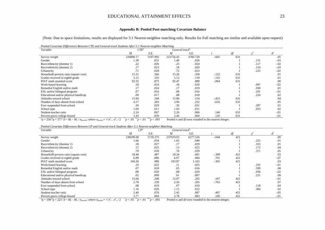
Covariate Balance
The pre-matching CTE vs. general-track sample showed statistically significant
differences on seven covariates. Discrepancies within the CP vs. general-track sample were even
greater, with 15 of the 20 covariates exhibiting significant differences (Appendix A). Both
Nearest-neighbor and Full matching successfully balanced samples across all covariates.
Hypothesis tests on the post-matching samples showed no remaining statistically significant
covariate differences in either CTE vs. general-track or CP vs. general-track samples (Appendix
B). Given journal space limitations, only results from Nearest-neighbor-based samples are shown
here. Results from Full matching are consistent with those from Nearest-neighbor matching and
are available upon request.
Curriculum Effects
Pooled chi-square statistics, standard errors, and Cramer’s V effect size coefficients were
calculated for all multiply-imputed datasets. Omnibus tests were significant for both CTE vs.
general-track and CP vs. general-track samples, with large and medium effect sizes, respectively.
Results were consistent across all multiply-imputed datasets (Table 3).
EDUCATIONAL ATTAINMENT EFFECTS 12
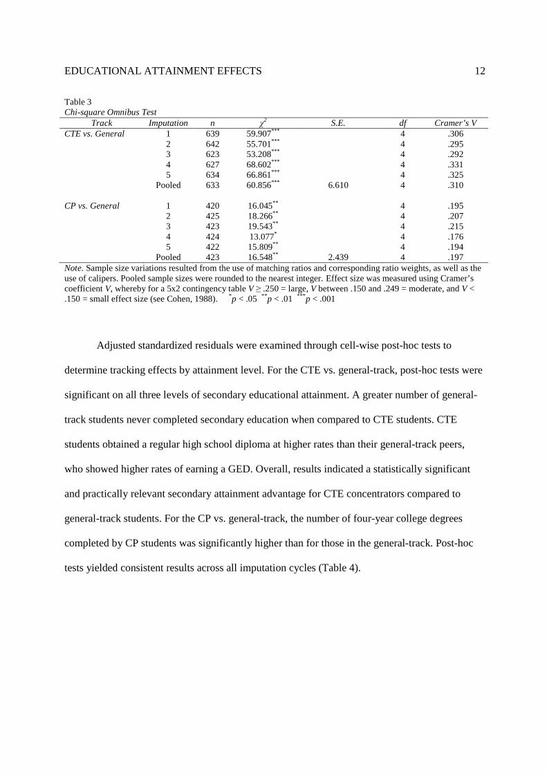
Table 3 Chi-square Omnibus Test
Track Imputation n χ2 S.E. df Cramer’s V
CTE vs. General 1 639 59.907*** 4 .306 2 642 55.701*** 4 .295 3 623 53.208*** 4 .292 4 627 68.602*** 4 .331 5 634 66.861*** 4 .325 Pooled 633 60.856*** 6.610 4 .310
CP vs. General 1 420 16.045** 4 .195 2 425 18.266** 4 .207 3 423 19.543** 4 .215 4 424 13.077* 4 .176 5 422 15.809** 4 .194 Pooled 423 16.548** 2.439 4 .197 Note. Sample size variations resulted from the use of matching ratios and corresponding ratio weights, as well as the use of calipers. Pooled sample sizes were rounded to the nearest integer. Effect size was measured using Cramer’s coefficient V, whereby for a 5x2 contingency table V ≥ .250 = large, V between .150 and .249 = moderate, and V < .150 = small effect size (see Cohen, 1988). *p < .05 ** p < .01 *** p < .001
Adjusted standardized residuals were examined through cell-wise post-hoc tests to
determine tracking effects by attainment level. For the CTE vs. general-track, post-hoc tests were
significant on all three levels of secondary educational attainment. A greater number of general-
track students never completed secondary education when compared to CTE students. CTE
students obtained a regular high school diploma at higher rates than their general-track peers,
who showed higher rates of earning a GED. Overall, results indicated a statistically significant
and practically relevant secondary attainment advantage for CTE concentrators compared to
general-track students. For the CP vs. general-track, the number of four-year college degrees
completed by CP students was significantly higher than for those in the general-track. Post-hoc
tests yielded consistent results across all imputation cycles (Table 4).

EDUCATIONAL ATTAINMENT EFFECTS 13
Table 4 Pooled Post-hoc Tests Attainment level CTE vs. General-track CP vs. General-track No HS diploma or GED -4.57* 4.57* -1.35 1.35 GED -5.68* 5.68* -2.31 2.31 Regular HS diploma 5.16* -5.16* -2.39 2.39 Two-year college degree 1.38 -1.38 .73 -.73 Four-year college degree .84 -.84 3.19* -3.19* Note. Adjusted standardized residuals exceeding z = ± 2.80 are statistically significant.
Sensitivity Analysis
One potential limitation of PSM is its inability to account for unobserved, yet causally-
relevant, concomitants. The exclusion of influential covariates may lead to hidden bias, for two
individuals with identical covariate values will have differential odds of treatment assignment
due to the impact of an unobserved covariate (Rosenbaum & Rubin, 1983). Sensitivity analysis
examines the degree to which effect estimates are undermined by hidden bias. Uncertainty about
the impact of unobserved covariates on the parameter estimate is captured by the parameter Γ,
and where eγ = 1 no hidden bias is present (for details on sensitivity analysis, readers are referred
to Rosenbaum, 2002). Results for CTE vs. general-track and CP vs. general-track yielded eγ =
2.00 and eγ = 1.94, respectively. Overall, sensitivity analysis supported the relative robustness of
the propensity score model and resulting inferences.
Discussion
CP
Results from this sample of 1996/97 ninth graders indicate that CP high school
concentrations prepare students for four-year college careers more effectively than general-track
curricula. This finding is unsurprising and corresponds with the extant literature. However,
conclusions about positive CP curriculum effects in general are premature given the absence of
differential high school dropout rates. The lack of a positive high school completion effect is
EDUCATIONAL ATTAINMENT EFFECTS 14
startling, for it is reasonable to expect the same track-based resource allocation mechanisms that
foster CP student attainment at the college level to provide advantages in high school.
The inefficiency of tracking mechanisms offers one possible explanation. CP curricula
are geared toward preparing academically able students for the transition to traditional four-year
colleges. However, myriad factors besides academic ability influence track assignment,
including teacher recommendations, personal choice, parental and peer influences, and school
resources. The influence of ancillary factors on tracking decisions may lead to frequent
misplacements of lower-achieving students into CP tracks where academic challenges can lead to
frustration and eventual dropout.
An alternative explanation may lie in the connection between disengagement and dropout
(see Goldschmidt & Wang, 1999). A recent study found that many high-achieving students
reported the perceived irrelevance of classes and resulting disengagement as their primary reason
for dropping out (Bridgeland, DiIulio, & Morison, 2006). It appears as if school disengagement
mechanisms affect CP and general-track students to similar degrees, irrespective of differences
in educational resources. While disengagement effects were not explored here, results indicate
that potential need to qualify blanket assumptions about the advantages of CP curricula for all
students.
CTE
Perkins 1990 sought to improve educational outcomes for traditionally work-bound youth
through career-oriented high school programs. Results from this study provide evidence for the
positive effects of CTE on high school completion. Even though career-oriented programs are
often more resource intensive, investments in CTE appear to generate substantive school

EDUCATIONAL ATTAINMENT EFFECTS 15
completion returns. The widespread stigmatization of high school CTE as a dumping ground for
unmotivated or incapable students should, therefore, be reconsidered.
The fact that general-track students obtained GEDs at significantly higher rates than their
CTE counterparts is a mixed blessing. Obtaining a GED is a preferred outcome for high school
dropouts because GED holders benefit from faster wage growth (Murnane, Willett, & Boudett,
1995) and exhibit a higher likelihood of enrolling in postsecondary education than non-GED
dropouts (Garet, Jing, & Kutner, 1996). However, GED holders who enroll in postsecondary
education are much less likely to complete their degree compared to those with a regular high
school diploma (Cameron & Heckman, 1993). GED holders also achieve lower average rates of
employment and income (Heckman, & LaFontaine, 2006). While obtaining a GED is beneficial,
it is clearly less desirable than obtaining a regular high school diploma.
Given that Perkins 1990 sought to position CTE more clearly as a pathway to
postsecondary education, the absence of any postsecondary attainment effects for this 1997
cohort of ninth-graders is quite sobering, especially at the two-year college level. As data for
more cohorts become available, future research should continue to assess transition effects from
high school CTE to postsecondary education.
Conclusion
Educational attainment effects of high school tracking were evaluated for a cohort of
ninth graders from the NLSY97. Results support a growing body of literature (e.g., Kim &
Bragg, 2008; Levesque et al., 2008; Plank et al., 2008) that considers CTE an effective option to
increase high school completion rates as a critical precursor to postsecondary educational
attainment.
EDUCATIONAL ATTAINMENT EFFECTS 16
References
Agodini, R., & Deke, J. (2004). The relationship between high school vocational education and
dropping out. Princeton, NJ: Mathematica Policy Research.
Agodini, R., Uhl, S., & Novak, T. (2004). Factors that influence participation in secondary
vocational education. Princeton, NJ: Mathematica Policy Research.
Arum, R., & Shavit, Y. (1995). Secondary vocational education and the transition from school to
work. Sociology of Education, 68, 187-204.
Barton, P. E. (2005). One-third of a nation: Rising dropout rates and declining opportunities.
Princeton, NJ: Educational Testing Service, Policy Information Center.
Barro, R. J. (2001). Human capital and growth. American Economic Review, 91, 12-17.
Berends, M. (1995). Educational stratification and students’ social bonding to school. British
Journal of Sociology of Education, 16, 327-351.
Bridgeland, J. M., DiIulio, J. J., & Morison, K. B. (2006). The silent epidemic: Perspectives of
high school dropouts. Washington, DC: Civic Enterprises.
Cameron, S. V., & Heckman, J. J. (1993). The nonequivalence of high school equivalents.
Journal of Labor Economics, 11, 1-47.
Castellano, M., Stringfield, S., & Stone III, J. R. (2003). Secondary career and technical
education and comprehensive school reform: Implications for research and practice.
Review of Educational Research, 73, 231-272.
Cellini, S. R. (2006). Smoothing the transition to college? The effect of Tech-Prep programs on
educational attainment. Economics of Education Review, 25, 394-411.
Cohen, J. (1988). Statistical power analysis for the behavioral sciences. Hillsdale, NJ: Erlbaum.

EDUCATIONAL ATTAINMENT EFFECTS 17
Crissey, S. R. (2009). Educational attainment in the United States: 2007. Washington, DC: U.S.
Census Bureau.
DeLuca, S., Plank, S., & Estacion, A. (2006). Does career and technical education affect college
enrollment? St. Paul, MN: University of Minnesota.
Foster, J. C. (2007). Assessment as a tool to evaluate the benefits of CTE. International Journal
of Vocational Education and Training, 15, 55-62.
Gamoran, A., & Mare, R. D. (1989). Secondary school tracking and educational inequality:
Compensation, reinforcement, or neutrality? American Journal of Sociology, 94, 1146-
1183.
Garet, M. S., Jing, Z., & Kutner, M. (1996). The labor market effects of completing the GED:
Asking the right questions. Washington, DC: American Institutes for Research.
Goldschmidt, P., & Wang, J. (1999). When can schools affect dropout behavior: A longitudinal
multilevel analysis. American Educational Research Journal, 36, 715-738.
Guo, S., & Fraser, M. W. (2010). Propensity score analysis: Statistical methods and
applications. Thousand Oaks, CA: Sage.
Hallinan, M. T. (2003). Ability grouping and student learning. Brookings Papers on Education
Policy, 1, 95-124.
Hanushek, E. A., Kain, J. F., Markman, J. M., & Rivkin, S. G. (2003). Does peer ability affect
student achievement? Journal of Applied Econometrics, 18, 527-544.
Heckman, J. J., & LaFontaine, P. A. (2006). Bias corrected estimates of GED returns. Journal of
Labor Economics, 24, 661-700.
Ho, D. E., Imai, K., King, G., & Stuart, E. A. (2007). Matchit (2.4-11) [computer software].
Retrieved from http://gking.harvard.edu/matchit

EDUCATIONAL ATTAINMENT EFFECTS 18
Ho, M. S., & Jorgenson, D. W. (1995). The quality of the U.S. work force, 1948-95. Cambridge,
MA: Harvard University.
Horn, L., & Kojaku, L. K. (2001). High school academic curriculum and the persistence path
through college: Persistence and transfer behavior of undergraduates 3 years after
entering 4-year institutions. Washington, DC: U.S. Department of Education.
Jones, J. D., Vanfossen, B. E., & Ensminger, M. E. (1995). Individual and organizational
predictors of high school track placement. Sociology of Education, 68, 287-300.
Kim, J., & Bragg, D. D. (2008). The impact of dual and articulated credit on college readiness
and retention in four community colleges. Career and Technical Education Research, 33,
133-158.
Kodrzycki, Y. K. (2002, June). Educational attainment as a constraint on economic growth and
social progress. Paper presented at the Federal Reserve Bank of Boston’s 47th annual
conference, Boston, MA.
Lee, V. E., & Ready, D. D. (2009). U.S. high school curriculum: Three phases of contemporary
research and reform. The Future of Children, 19, 135-156.
Leuven, E., & Sianesi, B. (2003). Psmatch2: Stata module to perform full Mahalanobis and
propensity score matching, common support graphing, and covariate imbalance testing.
[computer software]. Boston, MA: Boston College.
Levesque, K., Laird, J., Hensley, E., Choy, S. P., Cataldi, E. F., & Hudson, L. (2008). Career
and technical education in the United States: 1990 to 2005 (NCES 2008-035).
Washington, DC: U.S. Department of Education.
Lewis, T., & Cheng, S. (2006). Tracking, expectations, and the transformation of vocational
education. American Journal of Education, 113, 67-99.

EDUCATIONAL ATTAINMENT EFFECTS 19
Linver, M. R., Davis-Kean, P., & Eccles, J. E. (2002, April). Influences of gender on academic
achievement. Paper presented at the biennial meetings of the Society for Research on
Adolescence, New Orleans, LA.
Little, R. J. (1988). A test of missing completely at random for multivariate data with missing
values. Journal of the American Statistical Association, 83, 1198-1202.
Lucas, S. R., & Berends, M. (2002). Sociodemographic diversity, correlated achievement, and de
facto tracking. Sociology of Education, 75, 328-348.
MacDonald, P. L., & Gardner, R. C. (2000). Type I error rate comparisons of post hoc
procedures for I x J chi-square tables. Educational and Psychological Measurement, 60,
735-754.
Marsh, R. S., & Raywid, M. A. (1994). How to make detracking work. Phi Delta Kappan, 76,
314-317.
Murnane, R. J., Willett, J. B., & Boudett, K. P. (1995). Do high school dropouts benefit from
obtaining a GED? Educational Evaluation and Policy Analysis, 17, 133-147.
National Center on Education and the Economy. (1990). America's choice: High skills or low
wages! The report of the commission on the skills of the American workforce. Rochester,
NY: Author.
National Center on Education and the Economy. (2007). Tough choices or tough times: The
report of the new commission on the skills of the American workforce. San Francisco,
CA: Jossey-Bass.
National Commission on Excellence in Education. (1983). A nation at risk: The imperative for
reform. Retrieved from http://www.ed.gov/pubs/NatAtRisk/risk.html

EDUCATIONAL ATTAINMENT EFFECTS 20
Natriello, G., Pallas, A. M., & Alexander, K. (1989). On the right track? Curriculum and
academic achievement. Sociology of Education, 62, 109-118.
Neumark, D., & Rothstein, D. (2006). School-to-career programs and transitions to employment
and higher education. Economics of Education Review, 25, 374-393.
Organization for Economic Cooperation and Development. (2009). Education at a glance 2009.
Paris, France: Author.
Pittman, R. B. (1991). Social factors, enrollment in vocational/technical courses, and high school
dropout rates. Journal of Educational Research, 84, 288-295.
Plank, S. B., DeLuca, S., & Estacion, A. (2008). High school dropout and the role of career and
technical education: A survival analysis of surviving high school. Sociology of
Education, 81, 345-370.
Rasinski, K. A., & Pedlow, S. (1994). Using transcripts to study the effectiveness of vocational
education. Journal of Vocational Education Research, 19, 23-44.
Rosenbaum, P. R. (2002). Observational studies. New York, NY: Springer.
Rosenbaum, P. R., & Rubin, D. B. (1983). The central role of the propensity score in
observational studies for causal effects. Biometrika, 70, 41-55.
Rosenbaum, P. R., & Rubin, D. B. (1984). Reducing bias in observational studies using
subclassification on the propensity score. Journal of the American Statistical Association,
79, 516-523.
Rosenbaum, P. R., & Rubin, D. B. (1985). Constructing a control group using multivariate
matched sampling methods that incorporate the propensity score. The American
Statistician, 39, 33-38.
Rubin, D. B. (1987). Multiple imputation for nonresponse in surveys. New York, NY: Wiley.

EDUCATIONAL ATTAINMENT EFFECTS 21
Schafer, J. L. (1997). Analysis of incomplete multivariate data. Boca Raton, FL: Chapman &
Hall.
Schafer, J. L., & Graham, J. W. (2002). Missing data: Our view of the state of the art.
Psychological Methods, 7, 147-177.
Sidak, Z. (1967). Rectangular confidence regions for the means of multivariate normal
distributions. Journal of the American Statistical Association, 62, 626-633.
Silverberg, M., Warner, E., Fong, M., & Goodwin, D. (2004). National assessment of vocational
education: Final report to Congress. Washington, DC: U.S. Department of Education.
Sirin, S. R. (2005). Socioeconomic status and academic achievement: A meta-analytic review of
research. Review of Educational Research, 75, 417-453.
Snyder, T. D., Dillow, S. A., & Hoffman, C. M. (2009). Digest of education statistics 2008
(NCES 2009-020). Washington, DC: U.S. Department of Education.
Stone, J. R., & Aliaga, O. A. (2005). Career and technical education and school-to-work at the
end of the 20th century: Participation and outcomes. Career and Technical Education
Research, 30, 125-144.
Swanson, C. B. (2009). Closing the graduation gap: Educational and economic conditions in
America’s largest cities. Bethesda, MD: Educational Projects in Education Research
Center.
U.S. Department of Education. (2008). A nation accountable: Twenty-five years after a nation at
risk. Washington, DC: Author.
Van Buuren, S., & Groothuis-Oudshoorn, K. (2009). MICE: Multivariate imputation by chained
equations in R. Journal of Statistical Software, retrieved from
http://citeseerx.ist.psu.edu/viewdoc/download?doi=10.1.1.169.5745&rep=rep1&type=pdf

EDUCATIONAL ATTAINMENT EFFECTS 22
Appendix A: Pooled Pre-matching Covariate Balance Pooled Covariate Differences Between CTE and General-track Students (Pre-matching) Variable CTEa General-trackb M S.E. M S.E. t df χ2 dc Survey weight 228064.87 5098.743 203063.32 4086.552 -3.764*** 720 .29 Gender 1.37 .030 1.51 .023 1 12.576*** -.28 Race/ethnicity (dummy 1) .22 .026 .32 .022 1 7.901** -.23 Race/ethnicity (dummy 2) .16 .023 .22 .019 1 3.453 -.15 Urbanicity .71 .028 .72 .021 1 .128 -.02 Household poverty ratio (square root) 15.29 .352 14.45 .301 -1.761 720 .14 Grades received in eighth grade 5.15 .102 5.26 .075 .959 720 -.07 PIAT math standard score 92.82 .810 91.39 .670 -1.314 720 .10 Work-based learning .18 .024 .16 .017 1 .272 .04 Remedial English and/or math .17 .023 .19 .018 1 .409 -.05 ESL and/or bilingual program .07 .016 .11 .015 1 2.527 -.14 Educational and/or physical handicap .09 .018 .06 .011 1 1.842 .11 Attitudes toward school 15.88 .166 16.45 .135 2.613** 720 -.20 Number of days absent from school 4.10 .275 6.18 .401 3.641*** 720 -.30 Ever suspended from school .30 .028 .40 .023 1 8.184*** -.21 School type 1.03 .011 1.06 .011 1 1.779 -.14 Student-teacher ratio 2.22 .066 2.40 .050 2.113* 720 -.17 Percent peers college-bound 3.44 .058 3.37 .049 -.910 720 .07 an = 262 bn = 460 cd = Mt – Mc / σpooled; where σpooled = √ σ2
t + σ2c / 2 *p < .05 ** p < .01 *** p < .001
Pooled Covariate Differences Between CP and General-track Students (Pre-matching) Variable CPa General-trackb M S.E. M S.E. t df χ2 dc Survey weight 238530.25 5606.723 203063.32 4086.552 -4.937*** 662 .42 Gender 1.64 .034 1.51 .023 1 9.847** .26 Race/ethnicity (dummy 1) .17 .026 .32 .022 1 14.758*** -.35 Race/ethnicity (dummy 2) .15 .025 .22 .019 1 4.949* -.18 Urbanicity .77 .029 .72 .021 1 1.927 .12 Household poverty ratio (square root) 18.51 .458 14.45 .301 -7.468*** 662 .63 Grades received in eighth grade 6.91 .080 5.26 .075 -13.173*** 662 1.18 PIAT math standard score 105.11 1.007 91.39 .670 -11.303*** 662 .95 Work-based learning .10 .021 .16 .017 1 4.895* -.19 Remedial English and/or math .06 .017 .19 .018 1 16.917*** -.40 ESL and/or bilingual program .08 .019 .11 .015 1 1.446 -.10 Educational and/or physical handicap .01 .008 .06 .011 1 6.767** -.26 Attitudes toward school 15.00 .204 16.45 .135 5.941*** 662 -.50 Number of days absent from school 2.78 .250 6.18 .401 5.484*** 662 -.53 Ever suspended from school .07 .018 .40 .023 1 73.275*** -.84 School type 1.16 .026 1.06 .011 1 17.849*** .33 Student-teacher ratio 2.40 .073 2.40 .050 -.046 662 .01 Percent peers college-bound 3.78 .063 3.37 .049 -4.845*** 662 .42 an = 204 bn = 460 cd = Mt – Mc / σpooled; where σpooled = √ σ2
t + σ2c / 2 *p < .05 ** p < .01 *** p < .001
EDUCATIONAL ATTAINMENT EFFECTS 23
Appendix B: Pooled Post-matching Covariate Balance
(Note: Due to space limitations, results are displayed for 5:1 Nearest-neighbor matching only. Results for Full matching are similar and available upon request) Pooled Covariate Differences Between CTE and General-track Students After 5:1 Nearest-neighbor Matching Variable CTEa General-trackb M S.E. M S.E. t df χ2 dc Survey weight 226890.17 5197.992 222756.43 4760.720 -.605 631 .05 Gender 1.38 .031 1.40 .026 1 .131 -.03 Race/ethnicity (dummy 1) .22 .026 .23 .024 1 .117 -.02 Race/ethnicity (dummy 2) .17 .023 .18 .020 1 .154 -.03 Urbanicity .71 .028 .72 .023 1 .225 -.02 Household poverty ratio (square root) 15.31 .366 15.26 .358 -.122 631 .01 Grades received in eighth grade 5.15 .103 5.13 .118 -.142 631 .01 PIAT math standard score 92.55 .875 92.47 .888 -.064 631 .00 Work-based learning .18 .024 .18 .020 1 .097 -.02 Remedial English and/or math .17 .024 .17 .019 1 .030 .01 ESL and/or bilingual program .07 .016 .08 .016 1 .101 -.01 Educational and/or physical handicap .09 .017 .08 .018 1 .224 .02 Attitudes toward school 15.94 .168 15.84 .154 -.423 631 .04 Number of days absent from school 4.17 .283 3.96 .252 -.616 631 .05 Ever suspended from school .30 .029 .30 .031 1 .287 .01 School type 1.04 .011 1.03 .011 1 .033 .02 Student-teacher ratio 2.24 .067 2.26 .066 .146 631 -.01 Percent peers college-bound 3.43 .059 3.44 .060 .120 631 -.01 an = 256 bn = 377 cd = Mt – Mc / σpooled; where σpooled = √ σ2
t + σ2c / 2 *p < .05 ** p < .01 *** p < .001 Pooled n and df were rounded to the nearest integer.
Pooled Covariate Differences Between CP and General-track Students After 5:1 Nearest-neighbor Matching Variable CPa General-trackb M S.E. M S.E. t df χ
2 dc Survey weight 238299.00 5718.375 237919.03 6277.526 -.044 421 .00 Gender 1.66 .034 1.65 .040 1 .255 .01 Race/ethnicity (dummy 1) .18 .027 .17 .029 1 .103 .01 Race/ethnicity (dummy 2) .15 .025 .13 .025 1 .172 .04 Urbanicity .78 .030 .76 .029 1 .371 .05 Household poverty ratio (square root) 18.44 .487 18.24 .681 -.308 421 .03 Grades received in eighth grade 6.89 .086 6.97 .084 .701 421 -.07 PIAT math standard score 104.26 .980 103.87 1.102 -.305 421 .03 Work-based learning .10 .022 .11 .025 1 .192 -.01 Remedial English and/or math .07 .018 .05 .016 1 .599 .08 ESL and/or bilingual program .08 .020 .08 .020 1 .036 -.02 Educational and/or physical handicap .02 .009 .01 .007 1 .221 .09 Attitudes toward school 15.04 .208 15.07 .202 .107 421 -.01 Number of days absent from school 2.78 .239 2.56 .205 -.763 421 .07 Ever suspended from school .08 .019 .07 .018 1 .118 .04 School type 1.16 .026 1.15 .032 1 .384 .02 Student-teacher ratio 2.40 .076 2.45 .087 .497 421 -.05 Percent peers college-bound 3.77 .064 3.78 .083 .106 421 -.01 an = 198 bn = 225 cd = Mt – Mc / σpooled; where σpooled = √ σ2
t + σ2c / 2 *p < .05 ** p < .01 *** p < .001 Pooled n and df were rounded to the nearest integer.
Related Documents