simultaneous rayleigh and love wave acquisition for joint ...

USGS Award No. G18AP00064

Award Period: 07/01/2018 – 12/31/2019

SIMULTANEOUS RAYLEIGH AND LOVE WAVE ACQUISITION FOR JOINT

INVERSION OF MASW DATA

Principal Investigators:

Joseph Thomas Coe, Jr., Ph.D.

Department of Civil & Environmental Engineering

Temple University, 1947 North 12th Street, ENGR Building Room 518

Philadelphia, PA 19122-6018

Office: (215)204-6100, Fax: (215)204-4696, [email protected]

Graduate Student Researchers:

Trumer Wagner


Temple University, 1947 North 12th Street


[email protected]

Siavash Mahvelati


Temple University, 1947 North 12th Street


[email protected]

Final Technical Report

September 23, 2021

Project Website: https://sites.google.com/a/temple.edu/joseph-coe/research/usgs-g18ap00064

mailto:[email protected]



https://sites.google.com/a/temple.edu/joseph-coe/research/usgs-g18ap00064

i

ACKNOWLEDGEMENT OF SUPPORT AND DISCLAIMER

This material is based upon work supported by the U.S. Geological Survey under Grant No.

G18AP00064. The views and conclusions contained in this document are those of the authors and

should not be interpreted as representing the opinions or policies of the U.S. Geological Survey.

Mention of trade names or commercial products does not constitute their endorsement by the U.S.

Geological Survey.

The authors would like to thank former Temple University Ph.D. student Alireza Kordjazi and

former Temple University M.S.C.E. students Philip Asabere and Michael Senior for their

assistance during field testing. The authors would also like to thank Dr. Laura Toran for her input

regarding the location of the monitoring wells at the Temple University Ambler site. GISCO

provided the ESS Mini AWD source used in this study and their support for our research team is

greatly appreciated.

ii

TABLE OF CONTENTS

Abstract ........................................................................................................................................... 1

1. Introduction ................................................................................................................................. 2

1.1. Problem Statement ............................................................................................................... 3

1.2. Scope of Research ................................................................................................................ 4

1.3. Organization of Topics ........................................................................................................ 5

2. Background and Literature Review ............................................................................................ 8

2.1. Surface Wave Dispersion ..................................................................................................... 8

2.1.1 Development of Dispersion Curves ............................................................................... 8

2.2. Inversion ............................................................................................................................ 10

2.3. Uncertainty in Surface Wave Methods .............................................................................. 11

2.4. Fundamentals of the MASW Methodology ....................................................................... 12

2.4.1 MASW Field Procedures ............................................................................................. 12

2.4.2 Seismic Source ............................................................................................................. 13

2.4.3 Receivers ...................................................................................................................... 13

2.4.4 Acquisition Device....................................................................................................... 14

2.5. MASW Using Love Waves ............................................................................................... 15

2.6. Simultaneous Generation of Rayleigh and Love Waves ................................................... 15

2.7. Summary ............................................................................................................................ 17

3. Data Collection and Processing ................................................................................................ 22

3.1. Test Site ............................................................................................................................. 22

3.2. Field Testing ...................................................................................................................... 22

3.2.1 MASW Array Geometry .............................................................................................. 22

3.2.2 MASW Seismic Sources and Impact Plates ................................................................ 23

3.2.3 MASW Data Collection ............................................................................................... 23

3.2.4 Additional Seismic Geophysical Testing ..................................................................... 23

3.3. Data Processing .................................................................................................................. 24

3.3.1 Spectral Content and Relative Energy ......................................................................... 24

3.3.2 Signal to Noise Ratio (SNR) ........................................................................................ 24

iii

3.3.3 Dispersion Information ................................................................................................ 25

3.3.4 Inversion ...................................................................................................................... 26

4. Analysis of Results and Discussion .......................................................................................... 30

4.1. Frequency Content ............................................................................................................. 30

4.1.1 Rayleigh Waves ........................................................................................................... 31

4.1.2 Love Waves ................................................................................................................. 32

4.2. Relative Energy .................................................................................................................. 33

4.2.1 Rayleigh Waves ........................................................................................................... 34

4.2.2 Love Waves ................................................................................................................. 34

4.3. Signal-to-Noise Ratio (SNR) .............................................................................................. 35

4.3.1 Rayleigh Waves ........................................................................................................... 35

4.3.2 Love Waves ................................................................................................................. 35

4.4. Effects on Dispersion Information ..................................................................................... 36

4.4.1 Rayleigh Waves ........................................................................................................... 36

4.4.2 Love Waves ................................................................................................................. 37

4.5. Shear Wave Velocity (VS) Profiles .................................................................................... 38

4.5.1 Rayleigh Waves ........................................................................................................... 39

4.5.2 Love Waves ................................................................................................................. 40

4.5.3 Joint Inversion .............................................................................................................. 40

4.5.4 Comparisons Between Inversion Results..................................................................... 41

4.6. Summary ............................................................................................................................ 42

5. Conclusions ............................................................................................................................... 61

5.1. Goals of Project.................................................................................................................. 61

6. References ................................................................................................................................. 63

iv

LIST OF FIGURES

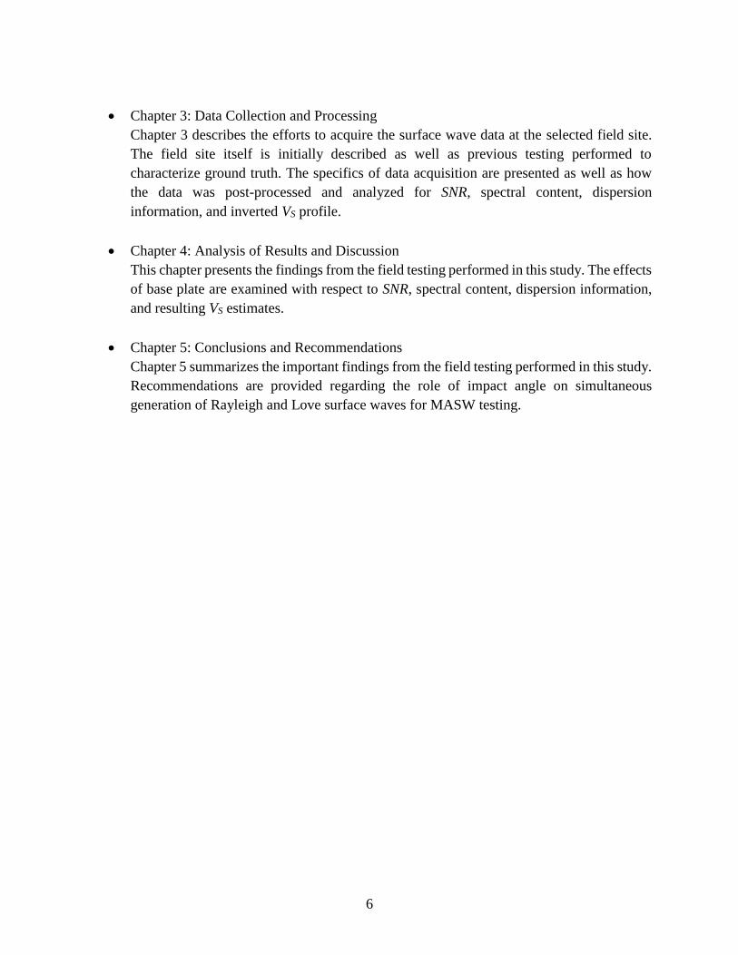
Figure 1.1. Direction of wave propagation for (a) Rayleigh and (b) Love waves. (Foti et al., 2017).

......................................................................................................................................................... 7

Figure 1.2. MASW data acquisition and resulting multichannel record with surface waves (adapted

from Olafsdottir et al., 2018). ......................................................................................................... 7

Figure 1.3. Generation of (a) Rayleigh waves, and (b) Love waves for MASW. .......................... 7

Figure 2.1. An illustration of the overall MASW procedure (Park et al., 2007). ......................... 18

Figure 2.2. Low f (long λ) waves (a) penetrate deeper than waves of higher f (shorter λ) (b) and

(c). (Ólafsdóttir, 2014). ................................................................................................................. 19

Figure 2.3. Flowchart and schematic of a typical local inversion algorithm (Olafsdottir, 2014). 20

Figure 2.4. Surface wave sources: (a) vertical source for Rayleigh waves; (b) angled wooden

source for Love waves; and (c) aluminum horizontal source for Love waves (Foti et al., 2017;

Haines 2007). ................................................................................................................................ 21

Figure 2.5. Galperin source and traditional angled base plate (Hausler et al., 2018). .................. 21

Figure 3.1. Temple Ambler campus site and survey line (Google Earth). ................................... 28

Figure 3.2. Ground truth model at TAB: (a) VS and VP profile; and (b) Rayleigh and Love wave

dispersion curves (Mahvelati, 2019). ............................................................................................ 28

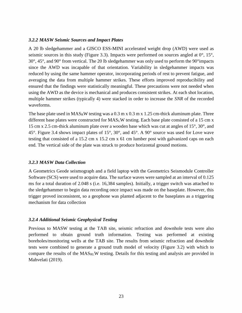
Figure 3.3. AWD positioned at impact angles of 15°, 30°, and 45° (Mahvelati, 2019). .............. 29

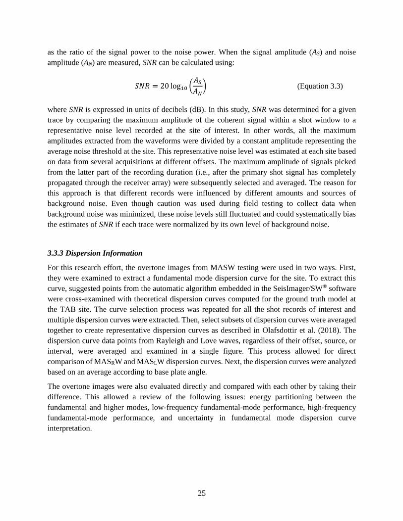
Figure 3.4. Custom impact sources for 15°, 30°, and 45° (Mahvelati, 2019). .............................. 29

Figure 4.1. Normalized Rayleigh power spectral density plots: (a) SO = -6dx, dx = 0.5 m; (b) SO

= -12dx, dx = 0.5 m; (c) SO = -6dx, dx = 1.0 m; (d) SO = -12dx, dx = 1.0 m; and (e) SO = -6dx,

dx = 1.5 m. .................................................................................................................................... 44

Figure 4.2. Normalized Love power spectral density plots: (a) SO = -6dx, dx = 0.5 m; (b) SO = -

12dx, dx = 0.5 m; (c) SO = -6dx, dx = 1.0 m; (d) SO = -12dx, dx = 1.0 m; and (e) SO = -6dx, dx =

1.5 m. ............................................................................................................................................ 45

Figure 4.3. Normalized relative energy graphs of Rayleigh waves: (a) SO = -6dx, dx = 1.5 m; (b)

SO = -6dx and -12dx, dx = 1.0 m; (c) SO = -6dx and -12dx, dx = 0.5 m. .................................... 46

Figure 4.4. Normalized relative energy graphs of Love waves: (a) SO = -6dx, dx = 1.5 m; (b) SO

= -6dx and -12dx, dx = 1.0 m; (c) SO = -6dx and -12dx, dx = 0.5 m. .......................................... 47

Figure 4.5. SNR plots of Rayleigh waves: (a) SO = -6dx, dx = 15 m; (b) SO = -6dx and -12dx, dx

= 1.0 m; (c) SO = -6dx and -12dx, dx = 0.5 m. ............................................................................ 48

Figure 4.6. SNR plots of Love waves: (a) SO = -6dx, dx = 1.5 m; (b) SO = -6dx and -12dx, dx =

1.0 m; (c) SO = -6dx and -12dx, dx = 0.5 m. ................................................................................ 49

v

Figure 4.7. Rayleigh wave dispersion curves compared to the 0° dispersion image: (a) SO = -6dx,

dx = 1.5 m; (b) SO = -6dx, dx = 1.0 m. ........................................................................................ 50

Figure 4.7 (cont.). Rayleigh wave dispersion curves compared to the 0° dispersion image: (a) SO

= -6dx, dx = 0.5 m; (b) SO = -12dx, dx = 1.0 m. .......................................................................... 51

Figure 4.7 (cont.). Rayleigh wave dispersion images compared to the 0° dispersion image: (e) SO

= -12dx, dx = 0.5 m. ...................................................................................................................... 52

Figure 4.8. Love wave dispersion images compared to the 0° dispersion image: (a) SO = -6dx, dx

= 1.5 m; (b) SO = -6dx, dx = 1.0 m. ............................................................................................. 53

Figure 4.8 (cont.). Love wave dispersion images compared to the 0° dispersion image: (c) SO = -

6dx, dx = 0.5 m; (d) SO = -12dx, dx = 1.0 m. .............................................................................. 54

Figure 4.8 (cont.). Love wave dispersion images compared to the 90° dispersion image: (e) SO =

-12dx, dx = 0.5. ............................................................................................................................. 55

Figure 4.9. Love wave dispersion curve generated by a 0° impact. ............................................. 55

Figure 4.10. Rayleigh inversion: (a) VS profiles; and (b) difference between inverted VS and

ground truth model VS. ................................................................................................................. 56

Figure 4.11. Love wave inversion: (a) VS profiles; and (b) difference between inverted VS and

ground truth model VS. ................................................................................................................. 57

Figure 4.12. Joint (Rayleigh and Love) inversion: (a) VS profiles; and (b) difference between

inverted VS and ground truth model VS. ....................................................................................... 58

vi

LIST OF TABLES

Table 4.1. Dominant frequencies in PSD plots for Rayleigh waves. ............................................ 59

Table 4.2. Shape factors (δ) from PSD plots for Rayleigh waves. ............................................... 59

Table 4.3. Dominant frequencies in PSD plots for Love waves. .................................................. 60

Table 4.4. Shape factors (δ) from PSD plots for Love waves. ..................................................... 60

1

Preface: The contents of this report have been adapted from: Wagner, T. (2020). Simultaneous

Rayleigh and Love Wave Generation for MASW Data. M.S. Thesis, Temple University. All project

files can be located at: https://sites.google.com/a/temple.edu/joseph-coe/research/usgs-

g18ap00064

ABSTRACT

The Multichannel Analysis of Surface Waves (MASW) method continues to increase in popularity

as a tool to characterize subsurface stiffness for site characterization. In typical MASW testing, a

linear array of geophones is used to record the surface waves generated from either vertical impacts

(Rayleigh waves) or horizontal impacts (Love waves). The phase velocity of these surface waves

is frequency-dependent in a vertically heterogeneous domain. This velocity-frequency dependency

(i.e., the dispersion curve) can be examined by applying wavefield transforms to the recorded raw

signals. An inversion algorithm is then implemented that attempts to locate the most probable shear

wave velocity (Vs) profile by matching the measured dispersion curve with theoretical dispersion

curves generated from forward modeling. This process is inherently nonlinear and ill-posed,

without a unique solution. As a result, considerable research has been devoted to inversion

algorithms for MASW. A number of studies have explored joint inversion of Rayleigh (MASRW)

and Love (MASLW) waves as a means to improve the accuracy of VS profiles. However, Rayleigh

and Love waves are routinely generated with a different source, which increases the length of time

for data acquisition to switch sources and reacquire data. No studies have systematically examined

the capabilities to develop simultaneous Rayleigh and Love waves from single sledgehammer

impacts on the same angled or vertical base plate source. Such an approach could encourage the

use of joint inversion schemes for MASW due to increased data acquisition efficiency. This

research project addresses this limitation by exploring optimal techniques for generating

simultaneous Rayleigh and Love waves (i.e., MASRLW) for use in joint inversion.

In this study, MASW field testing was performed to examine the effectiveness of an angled impact

for the simultaneous generation of Rayleigh and Love waves. Testing was performed at a baseball

field at the Temple Ambler campus site (TAB) approximately 24 km north of Center City

Philadelphia. A set of 24 geophone receivers was used to collect surface wave data from impacts

were performed at angles of 0°, 15°, 30°, 45°, and 90°. Both independent and joint inversions were

performed to produce VS profiles from the data. These VS profiles were subsequently compared to

ground truth information obtained from previous seismic refraction and downhole testing.

Additionally, the waveforms were examined with respect to spectral content and signal-to-noise

ratio and the dispersion images/curves were also compared. The results of this study demonstrated

that Love waves were significantly less affected by changes in impact angles when compared to

Rayleigh waves. Consequently, the optimal angle for simultaneous generation of Rayleigh and

Love waves may be biased more towards vertical. In this case, an impact angled at 15° from

vertical proved to be the best configuration for simultaneous generation of Rayleigh and Love

waves.



2

1. INTRODUCTION

The behavior of a soil is directly related to its geotechnical properties such as stiffness [i.e., small

strain shear modulus (G0)]. The G0 of a soil is a critical input parameter in several seismic design

applications, including estimation of ground motions and liquefaction potential. Typically, seismic

geophysical methods can be used to measure the shear wave velocity, VS, of the soil as a proxy for

G0 since it is directly related to G0 by mass density (G0 = ρV2).

Geophysical methods that estimate VS without drilling or invasive procedures (i.e., non-destructive

methods) have been increasingly used instead of traditional downhole and crosshole methods that

are more time intensive and costly. Surface wave analysis is a type of non-destructive geophysical

test that has been increasing in popularity since its development in the 1990s (Park et al., 1999;

Xia et al., 1999). A surface wave is a wave that results from the interaction between body waves

(P-waves/primary waves and S-waves/secondary waves) and propagates along the interface

between two different media (Figure 1.1). The two main types of surface waves are Rayleigh and

Love waves, which develop different particle motions in the underlying subsurface. The velocity

of both Rayleigh and Love waves are dependent on VS and can therefore be used to determine its

variation with depth at a site.

Rayleigh waves, the most fundamental of the surface waves, propagate in the vertical direction

and have a motion similar to that of a rolling ocean wave (Figure 1.1). The propagation of Rayleigh

waves depends on the wave frequency, VS, primary wave (P-wave) velocity (VP), layer thickness,

and soil density (ρ) (Xia et al., 1999). For Rayleigh waves, the amplitude of the associated motion

decays exponentially with depth. This motion becomes negligible within about one wavelength (λ)

from the surface, where λ is related to the frequency (f) of the wave and its phase velocity (V) by

λ = V / f. The decay of particle motion amplitude with depth for a Rayleigh wave cannot be

predicted a-priori without knowledge of the subsurface structure (Foti et al., 2017).

The particle motion of a Love wave is horizontal and transverse to the direction of wave

propagation (Figure 1.1). Love wave propagation depends on the same parameters as Rayleigh

waves, except for VP due to the purely horizontal particle motion. Love waves exist only in media

where there is a soft layer overlaying a stiffer layer, whereas Rayleigh waves always exist where

there is a free surface.

Surface wave testing has evolved from its origins with the early pioneering work of the 1950s (Van

de Pol 1951; Jones 1955) and single receiver approaches (Abbiss, 1981; Tokimatsu et al., 1991;

and Matthews et al., 1996) through multi-receiver approaches (e.g., Heisey et al., 1982). The most

recent breakthrough in surface wave testing came with the introduction of the Multichannel

Analysis of Surface Waves (MASW) method by Park et al. (1999) and Xia et al. (1999). In this

method, surface waves are generated at a site and recorded by a large number (i.e., 24 or more) of

receivers (Figure 1.2). The MASW method consequently allows for more efficient data acquisition

and for faster and more easily automated data processing. Noise sources, such as inclusion of body

waves and reflected/scattered waves can be more easily filtered out, which can lead to a more

accurate VS profile than other surface wave methods (Ólafsdóttir, 2014). Furthermore, observation

3

of more complex wave propagation characteristics and generation of two (or three) dimensional

velocity profiles becomes possible and economically feasible.

All surface wave methods attempt to decipher the characteristics of the subsurface by examining

the dispersive nature of the recorded surface waveforms. Dispersion refers to the phenomenon

whereby different f components of the waveforms (i.e., different λ) “sample” different depths of

the subsurface and therefore propagate at different V. Once the dispersion behavior of the

waveforms has been established at the site, an inversion problem is solved to generate a subsurface

velocity model. The inversion proceeds by attempting to match the acquired dispersion

information with theoretical dispersion information from forward modeling with various trial

subsurface velocity profiles.

1.1. Problem Statement

Traditionally, MASW has been performed using the generation of Rayleigh waves (i.e., MASRW

or MARW). The application of Love waves to MASW (MASLW or MALW) has only recently

gained traction (Yong et al., 2013) despite knowledge of their existence since the start of the 20th

century (Love, 1911). There are a number of advantages presented by use of Love waves in surface

wave surveys, including independence from VP, higher signal-to-noise ratio (SNR), and a more

stable inversion process (Xia et al., 2012). Love wave surveys can be performed to supplement

Rayleigh wave surveys. In this scenario, two separate VS profiles would be generated that could be

used to increase the accuracy of the predicted subsurface characteristics and bracket the final

solution. Alternatively, the two sets of dispersion information from recordings of Rayleigh and

Love waveforms can be jointly inverted. The purpose of joint inversion is to develop one objective

function to optimize during the inversion process. This singular objective function is jointly

developed from the individual objective functions representing the Rayleigh and Love wave data

sets. In this manner, joint inversion can reduce the number of acceptable subsurface velocity

models and can produce mutually consistent estimates because the results must explain all data

simultaneously (Vozoff and Jupp, 1975; Julia et al., 2000).

Whether Love waves and Rayleigh waves are independently or jointly inverted, the supplemental

use of Love waves for MASW is desirable to increase the accuracy of predicted subsurface

stiffness. However, Rayleigh and Love waves propagate most strongly in directions perpendicular

to one another – Rayleigh waves in the vertical direction and Love waves in the horizontal

direction. Consequently, Rayleigh and Love waves are typically generated by separate vertical and

horizontal impacts on the ground surface, respectively (Figure 1.3). A metallic base plate is

typically used to couple the impact energy and improve its transfer into the underlying ground

surface. The configuration of this base plate is different between Rayleigh and Love wave

generation due to the orientation/polarization of the impact (Figure 1.3). Therefore, Rayleigh and

Love waves are almost always generated and recorded separately if both sets of waves are used.

This results in conducting twice as many impacts to obtain the data necessary for the analysis of

both Rayleigh and Love waves. So, while MASW using both Rayleigh and Love waves (i.e.,

4

MASRLW or MARLW) may increase the accuracy of the velocity profile compared to single-

component MASW, the time and effort of data collection is significantly increased and both sets

of waves are rarely used.

If Rayleigh and Love waves are generated and recorded simultaneously from the same impact, the

efficiency of the data acquisition process is drastically improved. In return, MASRLW becomes a

more appealing process due to the benefit of increased accuracy with minimal changes to analysis

time and/or effort. However, very little research has been performed to systematically analyze the

most effective impact angle with which to simultaneous generate Rayleigh and Love waves as

highlighted in the literature review of Chapter 2. Consequently, no guidance exists about how to

design the most appropriate MASRLW survey, particularly with respect to the manner with which

the seismic source is used to simultaneously generate the waves.

1.2. Scope of Research

Given the aforementioned gaps in the literature regarding simultaneous generation of Rayleigh

and Love waves, this research project addresses the following issues:

1. What is the optimal angle of impact for simultaneous generation of Rayleigh and Love

wave generation.

2. How effective are vertical impacts for generating simultaneous Rayleigh and Love waves.

This research efforts aims to advance the field of geophysical subsurface investigation, specifically

MASW testing. By improving the accuracy and data collection times of MASW, the procedure

will continue to increase in popularity and offer an appealing alternative to traditional geotechnical

subsurface investigation methods.

As noted previously, Rayleigh waves are typically generated using a vertical impact (i.e., 0° angle

from a line drawn vertically from the ground surface) of a sledgehammer (Figure 1.3). Love waves

are typically generated using a completely horizontal impact (i.e., 90° angle from a line drawn

vertically from the ground surface) (Figure 1.3). Any deviations from these “ideal” Rayleigh and

Love impact sources and angle should result in negative effects on several characteristics of the

recorded signals, including SNR, spectral content, and perhaps the accuracy of the resulting VS

profile. Selection of an optimal angle of impact should therefore represent an intermediate angle

between 0° to 90° that least negatively affects both types of waveforms.

In theory, an impact angle of 45° should represent the optimal angle for the simultaneous

generation of Rayleigh and Love waves since approximately half of the impact energy is converted

into Rayleigh waves and the other half Love waves. Impact angles closer to vertical would likely

generate a higher proportion of Rayleigh wave energy at the expense of Love wave energy. Impact

angles closer to horizontal would likely improve Love wave performance at the expense of

Rayleigh waves. However, it is not clear whether there is some aspect of either Rayleigh or Love

wave generation that reduces their sensitivity to the impact angle. In such a scenario, the optimal

5

impact angle may be controlled by one waveform over another. For example, if Love waves are

less sensitive to impact angles and only a minimum threshold is needed to generate adequate Love

wave energy, the optimal impact angle would be controlled by a bias towards generating more

Rayleigh wave energy.

In this study, the optimal impact angle was examined on the basis of SNR, relative energy,

frequency content, and dispersion information. Additionally, the final VS profiles created by angled

impacts were compared with VS profiles produced from ground truth information. The goal of this

research effort is to identify an impact angle that generates VS profiles that compare favorably to

those created from traditional MASRW and MASLW techniques and to those representing ground

truth. Based on these efforts, it may be possible to provide prescriptive guidance for optimal field

efforts with simultaneous generation in the future.

In addition to attempting to identify the optimal impact angle for simultaneous generation of

Rayleigh and Love waves, this study also evaluates the effectiveness of vertical impacts for this

same purpose. The research question being tackled in this phase of the study is whether a purely

vertical impact can generate sufficient Love wave energy for analysis in either an independent

inversion process or joint inversion algorithm. Though it may seem odd to consider that a purely

vertical impact may generate horizontally-polarized wave energy, gravitational forces may indeed

cause a very small proportion of a vertical impact to convert into some form of horizontal wave

propagation. Vertical impacts for Love waves will likely never produce the same quality data as

horizontal impacts, but usable data may still be obtained from such strikes. As noted in the Chapter

2 literature review, there is some empirical evidence from other studies that such a small

component of horizontally-polarized waveform energy is measurable using modern receivers and

data acquisition systems. Consequently, it may be possible to forgo the use of specialized

horizontal base plates in favor of a standard metallic base plate as used with Rayleigh wave

generation. This would simplify data acquisition and further encourage the use of MASRLW in lieu

of MASRW and/or MASLW. This task was also evaluated based on SNR, relative energy, frequency

content, dispersion information, and accuracy of the inverted VS profile.

1.3. Organization of Topics

The scope of this research is to examine the role of impact angles on the simultaneous generation

of Rayleigh and Love waves for MASW testing. The body of this report is organized into the

following chapters:

• Chapter 2: Background and Literature Review

This chapter summarizes the relevant general background on surface wave testing and the

specifics related to the MASW methodology itself. A discussion is provided regarding the

role of data acquisition, post-processing, and subsequent inversion on MASW results. A

comprehensive literature review is also presented that discusses relevant studies on

simultaneous generation of Rayleigh and Love waves.

6

• Chapter 3: Data Collection and Processing

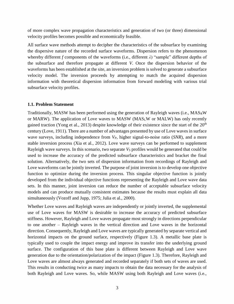
Chapter 3 describes the efforts to acquire the surface wave data at the selected field site.

The field site itself is initially described as well as previous testing performed to

characterize ground truth. The specifics of data acquisition are presented as well as how

the data was post-processed and analyzed for SNR, spectral content, dispersion

information, and inverted VS profile.

• Chapter 4: Analysis of Results and Discussion

This chapter presents the findings from the field testing performed in this study. The effects

of base plate are examined with respect to SNR, spectral content, dispersion information,

and resulting VS estimates.

• Chapter 5: Conclusions and Recommendations

Chapter 5 summarizes the important findings from the field testing performed in this study.

Recommendations are provided regarding the role of impact angle on simultaneous

generation of Rayleigh and Love surface waves for MASW testing.

7

Figure 1.1. Direction of wave propagation for (a) Rayleigh and (b) Love waves. (Foti et al., 2017).

Figure 1.2. MASW data acquisition and resulting multichannel record with surface waves (adapted from

Olafsdottir et al., 2018).

Figure 1.3. Generation of (a) Rayleigh waves, and (b) Love waves for MASW.

(a)

(b)

8

2. BACKGROUND AND LITERATURE REVIEW

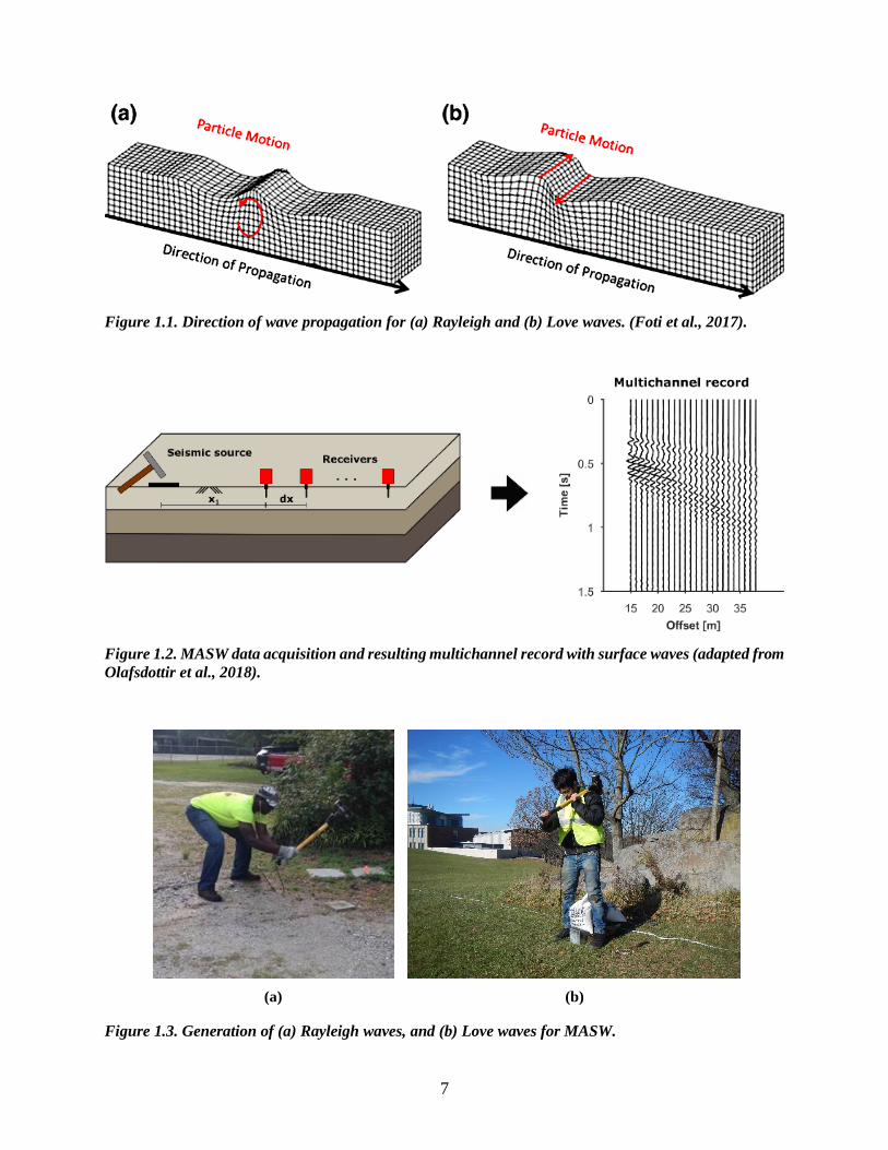
Surface wave analysis aims to generate a shear wave velocity (VS) profile by solving an inverse

problem of model parameter identification based on an experimental dispersion curve. Typical

analysis procedures consist of three sequential steps: (1) acquisition of seismic data; (2) data post-

processing (dispersion curve estimation); and (3) inversion (model parameter optimization) (Foti

et al., 2017) (Figure 2.1). The following sections describe these steps in more detail. More specific

details of the MASW methodology adopted for this study is subsequently presented.

2.1. Surface Wave Dispersion

Surface wave propagation is controlled by dispersion; that is, waves of different wavelengths (λ)

“sample” different depth ranges and the corresponding phase velocity (V) depends on the material

properties of the subsurface within that wave’s propagation range (Foti et al., 2017). Love waves

are inherently dispersive while Rayleigh waves are only dispersive in a heterogenous media. This

means that the V of wave propagation is dependent on the frequency (f) of the wave. Surface wave

methods measure this f dependency of surface wave V (i.e. dispersion). After data collection and

processing, the first step toward creating a VS profile is the generation of a dispersion image. The

end product is a VS profile that is estimated using an inversion process to match field dispersion

measurements to theoretical curves generated using forward modeling.

The parameters f, V, and λ are related by the equation f = V / λ. Therefore, for the same V, lower f

equates to a higher (longer) λ, and vice-versa. Long λ surface waves penetrate more deeply into

the subsurface than short λ surface waves (Figure 2.2). Since the V of wave propagation in the

Earth tends to increase with increasing depth, the longer λ (low f) waves can travel faster than the

shorter λ (high f) waves. These relationships are used to generate the dispersion curve for a

subsurface.

2.1.1 Development of Dispersion Curves

One of the most important aspects of surface wave testing is the development of a dispersion curve

based on the input seismic wave. The dispersion curve characterizes the V-f behavior of the surface

waves at a site. Several signal analysis tools can be used for the extraction of dispersion curves

from experimental data. Methods that can be implemented to provide an automated extraction of

the dispersion curve are helpful, but a careful assessment of obtained information is necessary

(Foti et al., 2017). Most of these techniques assume a one-dimensional medium below the array

(horizontally stratified, V only varies with depth), and plane wave propagation (the receiver array

is far enough from the seismic source so that the surface wave is fully developed and the wave

front can be approximated by a plane) (Foti et al., 2017).

9

Visual inspection of the dispersion curve can provide an indication of the expected trends in the

VS profile. A dispersion curve with a smooth and continuous decrease of V for increasing f is

typically associated with simple stratigraphic conditions with VS consistently increasing with depth

(i.e. a normally dispersive subsurface). The presence of a dip in the experimental dispersion curve

can indicate the presence of an inverse layering at some depth (i.e. a soft layer below a stiffer one)

(Foti et al., 2017).

Several techniques exist for the analysis of the seismic data and creation of a dispersion image.

The multichannel record, which is in the time (t)-space (x) domain, is converted into either the

frequency (f)-wavenumber (k) or the frequency (f)-phase velocity (Cf) domain (e.g., McMechan

and Yedlin 1981; Park et al. 1998). The resulting dispersion image (Figure 2.1) represents the

patterns of energy accumulation resulting from the wavefield transformation.

2.1.1.1 Phase-Shift Method

The quality of the dispersion image generated by the phase-shift method (Park et al., 1998) is

superior to those obtained by the other aforementioned methods. Therefore, the phase-shift method

was used throughout this research effort to develop dispersion images. In the phase-shift method,

the dispersion properties of all types of waves contained in the recorded data are visualized in the

f-Cf-transformed energy (summed wave amplitude) domain (Olafsdottir, 2014). The phase-shift

method can be divided into three steps:

1. Fourier transformation and amplitude normalization

2. Dispersion imaging

3. Extraction of dispersion curves

As described by Park et al. (1998), in the phase-shift method, the raw field data in the offset-time

domain are first transformed via Fast Fourier Transform (FFT) into individual f components

(offset-frequency domain), and then amplitude normalization is applied to each component. The

new domain is a combined function of amplitude and phase spectra. The amplitude part of the

offset-frequency domain contains properties of attenuation, spherical divergence, and related

information, whereas the phase spectra explain the wave dispersion (Park et al. 1998).

Next, for each offset at a given Cf and f in a certain range, the phase shift required to compensate

for the time delay corresponding to that specific offset is calculated and applied. Next, at particular

f intervals (i.e., 1 Hz intervals), the transformed traces (offsets) are aggregated using an integral

function (Park et al. 1998). At each f, there is a Cf providing a maximum value for the accumulated

energy presented by the integral. This represents the Cf (or V in previous terminology) at that

particular frequency. The display of all summed energy in the f-Cf space highlights a pattern of

energy accumulation that represents the dispersion curve.

10

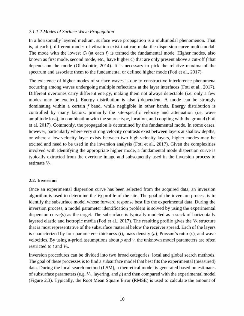
2.1.1.2 Modes of Surface Wave Propagation

In a horizontally layered medium, surface wave propagation is a multimodal phenomenon. That

is, at each f, different modes of vibration exist that can make the dispersion curve multi-modal.

The mode with the lowest Cf (at each f) is termed the fundamental mode. Higher modes, also

known as first mode, second mode, etc., have higher Cf that are only present above a cut-off f that

depends on the mode (Olafsdottir, 2014). It is necessary to pick the relative maxima of the

spectrum and associate them to the fundamental or defined higher mode (Foti et al., 2017).

The existence of higher modes of surface waves is due to constructive interference phenomena

occurring among waves undergoing multiple reflections at the layer interfaces (Foti et al., 2017).

Different overtones carry different energy, making them not always detectable (i.e. only a few

modes may be excited). Energy distribution is also f-dependent. A mode can be strongly

dominating within a certain f band, while negligible in other bands. Energy distribution is

controlled by many factors: primarily the site-specific velocity and attenuation (i.e. wave

amplitude loss), in combination with the source type, location, and coupling with the ground (Foti

et al. 2017). Commonly, the propagation is determined by the fundamental mode. In some cases,

however, particularly where very strong velocity contrasts exist between layers at shallow depths,

or where a low-velocity layer exists between two high-velocity layers, higher modes may be

excited and need to be used in the inversion analysis (Foti et al., 2017). Given the complexities

involved with identifying the appropriate higher mode, a fundamental mode dispersion curve is

typically extracted from the overtone image and subsequently used in the inversion process to

estimate VS.

2.2. Inversion

Once an experimental dispersion curve has been selected from the acquired data, an inversion

algorithm is used to determine the VS profile of the site. The goal of the inversion process is to

identify the subsurface model whose forward response best fits the experimental data. During the

inversion process, a model parameter identification problem is solved by using the experimental

dispersion curve(s) as the target. The subsurface is typically modeled as a stack of horizontally

layered elastic and isotropic media (Foti et al., 2017). The resulting profile gives the VS structure

that is most representative of the subsurface material below the receiver spread. Each of the layers

is characterized by four parameters: thickness (t), mass density (ρ), Poisson’s ratio (ν), and wave

velocities. By using a-priori assumptions about ρ and ν, the unknown model parameters are often

restricted to t and VS.

Inversion procedures can be divided into two broad categories: local and global search methods.

The goal of these processes is to find a subsurface model that best fits the experimental (measured)

data. During the local search method (LSM), a theoretical model is generated based on estimates

of subsurface parameters (e.g. VS, layering, and ρ) and then compared with the experimental model

(Figure 2.3). Typically, the Root Mean Square Error (RMSE) is used to calculate the amount of

11

misfit between the theoretical and experimental model. Theoretical models are generated until

there is an acceptably low difference between the experimental and theoretical models. LSM are

efficient in regard to both time and computational power, but because the solution is based on a

pre-defined starting model, there is a risk of the model becoming stuck at a local minimum during

the inversion process (Socco et al., 2010). The choice of the initial model is therefore crucial in

LSM because the result of the inversion may be strongly dependent on the adopted initial model

(Foti et al., 2017).

In global search methods (GSM), a probability density distribution is defined for each model

parameter, creating a range for potential models (Foti et al., 2017). A conventional approach to

global search is to randomly generate parametric sets within the previously specified range. In

contrast with the single model produced by local search methods, GSM generate a set of acceptable

profiles. GSM require significantly more time and computational power compared to local search

methods but have the potential to produce more accurate VS profiles.

2.3. Uncertainty in Surface Wave Methods

A key issue with surface waves is the uncertainty associated with the inversion process. The final

model is affected by solution non-uniqueness, as several theoretical dispersion curves may provide

a similar match to the experimental curve (Foti et al., 2017). The result of the inversion process is

inherently ill-posed (the solution’s behavior does not depend continuously on the initial

conditions), non-linear (the change in the solution is not proportional to the change in the initial

conditions), and mix-determined (insufficient data is available to constrain certain model

parameters) (Cox and Teague, 2016).

GSM mitigate some of the issues of uncertainty associated with MASW and are recommended to

be used when no a-priori information is available. These methods avoid assumptions of linearity

between the observables and the unknown and offer a way of handling the non-uniqueness of the

inversion problem (Socco et al., 2010). GSM are gaining popularity due to continued

improvements in computational power and the development of several optimization methods.

These optimization methods utilize simulated annealing (SA) or apply genetic algorithms (GAs)

to reduce the number of simulations required to obtain a best fit.

A-priori information about the subsurface site conditions may also increase the accuracy of the VS

profile by restricting the model parameters to a range of reasonable values. Any available a-priori

information should be factored into the initial parameterization for both local and global search

methods. Useful information can be retrieved from previous studies, geological maps, borehole

data, or other geophysical tests. Unfortunately, a-priori site information is often difficult to obtain,

especially at depths where surface wave testing resolution and accuracy suffers. Consequently,

many MASW inversion are performed in a “blind” fashion.

The inclusion of higher modes during the inversion process presents another means of obtaining a

more accurate VS profile. Typically, a fundamental mode (i.e., lowest Cf for a given f) is selected

12

from the peak intensity values plotted in the dispersion image. However, there has been significant

debate regarding the importance of higher modes of propagation. It is now recognized that higher

modes play a significant role in the inversion process and failing to consider them may cause errors

in several situations (Socco et al. 2010 and Xia et al. 2000). Joint inversion of the fundamental and

higher modes produces additional independent information that is useful to combat solution non-

uniqueness. While several methods have been proposed to account for higher modes during

inversion, the procedures are not standardized or implemented in most commercial codes (Foti et

al., 2017).

2.4. Fundamentals of the MASW Methodology

During MASW, surface waves are generated by active methods, such as a sledgehammer striking

a baseplate, or by passive methods, such as ambient traffic vibrations (Figure 2.1). These active

and passive sources provide various levels of excitation and signal quality. Typically, a larger,

heavier source generates longer λ while a smaller, lighter source produces shorter λ. A receiver

such as a geophone senses the ground vibration generated by the surface wave and converts that

vibration into electric current via a mass-spring system enclosed in a magnet. The f-amplitude

relationship of a geophone is called the “response curve” and is determined primarily by the size

of the hanging mass and stiffness of the spring. Vertical geophones are used for Rayleigh wave

surveys while horizontal geophones are used for Love wave surveys. The raw waveforms are

recorded by a field device, typically a seismograph. The data is then processed, analyzed, and used

to create a VS profile of the subsurface. These steps are further discussed in the following sections.

2.4.1 MASW Field Procedures

The first step toward generating a VS profile with MASW is data collection. Surface waveforms

may be collected by two primary methods: active and passive surveys. During an active survey,

surface waves are generated by sledgehammer strikes on a baseplate. In passive surveys, ambient

surface waves are collected from background seismic sources such as traffic. The depth of

investigation is directly proportional to the longest measurable λ (lowest f) and the minimum

resolvable layer thickness is related to the shortest λ (highest f) (Xia et al., 1999; Park et al., 2002).

The maximum measured λ depends on (Foti et al., 2017):

• The frequency content of the propagating seismic signal

• The array layout aperture used for recording

• The frequency bandwidth of the sensors

• The velocity structure of the site

Data acquisition up to a depth of 30 m using a sledgehammer is typically only possible for stiff

sites; soft sites generally have a maximum investigation depth of 15-20 m with a sledgehammer.

Background ambient surface wave vibrations can typically investigate deeper strata because they

13

generally contain lower f content than even the largest active seismic sources. Consequently, it is

recommended that both active and passive surveys be performed at sites where the target

investigation depth is greater than approximately 20-25 m (Foti et al., 2017). Field acquisition

parameters can have a significant impact on data quality and are, therefore, designed to adapt the

above characteristics to the project objective.

2.4.2 Seismic Source

During active MASW testing, surface waves are generated by a seismic source. This source must

provide an adequate signal-to-noise (SNR) ratio over the required frequency band, given the target

investigation depth. Since wavelength is a function of both f and V (i.e., Cf), it is necessary to make

initial estimates regarding the expected velocity range to define the required f band of the source.

At a soft site, lower f will be necessary to achieve the same investigation depth as at a stiff site.

Vertical operated shakers or vertical impact sources are typically used for surface wave testing.

Shakers provide accurate control of f and a very high SNR in the optimal frequency band of

operation. However, they are also very expensive and difficult to manage. Impact sources, on the

other hand, are much cheaper and still enable as efficient data acquisition as shakers over a wide

frequency band.

The cheapest and most common source is a sledgehammer striking a metal plate or directly on the

ground surface. However, the sledgehammer is typically limited to f > 8-10 Hz, which limits

investigation depth to a few tens of meters (typically no more than 30 m). Accelerated weight drop

(AWD) sources can improve the low f response and investigation depth since they typically

generate more energy than sledgehammer sources. Additionally, they offer repeatability with

respect to the energy introduced by each impact. However, AWD units are large, cumbersome to

deploy, and expensive. As with any active source, the SNR can be improved by stacking multiple

shots. Additionally, the energy output of the sledgehammer is dependent on its operator.

Precautions must be taken to ensure the quality of data is not altered by varying sledgehammer

strikes.

A trigger switch is typically used to begin data acquisition. This trigger switch may be attached to

the source (e.g. taped to the sledgehammer) or placed very close to the source so as to trigger

before the surface waves reach the geophone array.

2.4.3 Receivers

Geophones are commonly used as receivers for acquisition of Rayleigh and Love wave data during

MASW testing. The geophone must be capable of recording vertical motions to acquire Rayleigh

waveforms and horizontal geophones are used to record Love waves. Single component geophones

(i.e., only vertical or horizontal polarization) are commonly used, though multi-component

geophones are available and decrease data acquisition times for investigations where both

14

Rayleigh and Love waves are used. MASW is typically performed using 24 or 48 geophones,

though this is limited by site logistics and costs more than anything. The geophones may be planted

into soft to medium-stiff ground via spikes or placed on flat bases (typically metallic).

The natural f of the geophones must be adequate to sample the expected frequency band of surface

waves without distortions due to sensor response. Generally, for shallow targets (e.g. 30 m) 4.5 Hz

geophones are typically used for both MASRW and MASLW. For active surveys, the geophones

are equally spaced in a straight line from the source. During passive surveys, it is common practice

to arrange the geophones in a 2D array on the ground surface in order to capture ambient vibration

from any direction. However, the straight-line configuration is also used for passive surveys with

longer receiver spacings to adequately capture the longer λ for the ambient vibrations. Lower f

geophones (e.g., 1 Hz) may be used to acquire the longer λ (i.e., lower f) signals.

The array length for active surveys should be adequate for a reliable sampling of long λ, which are

associated with the propagation of low-frequency components. A rule of thumb is to have the array

length at least equal to the maximum desired λ, which corresponds to approximately twice the

desired investigation depth (Foti et al., 2017). The spacing between adjacent receivers should be

adequate to reliably sample short λ, which are associated with the high-frequency waves necessary

to constrain the near-surface solution. Suggested values for receiver spacing range from 0.5 m to

4 m (Foti et al., 2017).

The source position should be selected as a compromise between the need to avoid near-field

effects, which prevent surface waves from fully developing, and the opportunity to preserve high-

frequency components that rapidly degrade with distance as a result of far-field effects. It may be

useful to repeat MASW acquisition with multiple source offsets and source types to ensure high-

quality data. Stacking of multiple shots is also good practice, as it increases the SNR and therefore

improves the phase velocity estimation.

2.4.4 Acquisition Device

A variety of devices may be used to digitize the analog output from the geophones and record

signals. The most common choice is a multichannel seismograph, which is specifically designed

for seismic acquisition. Typically, one or two seismographs are connected to the geophone arrays

(the number depends on the number of geophones used).

During data recording, the sampling rate affects the retrieved f. The sampling frequency (fs) should

be at least equal to twice the maximum f of the propagating signal. For surface wave analysis, a

sampling interval of 2 ms (fs = 500 Hz) is adequate for most situations. The recording time window

must be long enough to record the entire surface wave train. A window of 2 seconds is usually

sufficient for most arrays, but it is suggested to use longer windows when testing on soft sediments

and/or longer arrays. Additionally, passive surveys require much longer acquisition times to ensure

adequate acquisition of multi-directional ambient vibrations.

15

2.5. MASW Using Love Waves

Surface wave methods, such as SASW and MASW, are proven non-destructive geophysical

techniques capable of generating accurate VS profiles (Yong et al., 2013; Park et al., 2007; and Foti

et al. 2017). Significant efforts have been devoted to the research and application of Rayleigh

waves in MASW (MASRW). Although Love waves have been utilized in seismological studies for

many years (e.g. Lay and Wallace, 1995), the application of Love waves to MASW (MASLW) has

only recently gained traction (Yong et al., 2013). Two of the earliest known applications of Love

waves for the characterization of VS are by Mari (1984) and Song et al. (1989). More recent

publications on MASLW include Safani et al. (2005), Eslick et al. (2007), Pei (2007), Xia et al.

(2012), Yong et al. (2013), Yin et al. (2014), and Mahvelati and Coe (2017).

These research efforts indicate that Love waves are particularly well-suited for sites with sufficient

stiffness contrast near the subsurface. Generally, Rayleigh waves can penetrate approximately 1.3-

1.4 times deeper than Love waves with the same λ (Song et al., 1989). However, this applies when

only considering fundamental mode behavior as both waves demonstrate similar penetration

depths at higher modes (Yin et al., 2014). As outlined by Xia et al. (2012), Love wave inversion

has the following advantages relative to traditional Rayleigh wave inversion:

1. The independence from VP makes Love wave dispersion curves simpler than Rayleigh

waves and reduces the non-uniqueness of the inversion process.

2. The dispersion images of Love-wave energy have a higher SNR and more focus than those

generated from Rayleigh waves, which makes picking phase velocities easier and more

accurate.

3. The inversion of Love wave dispersion curves is less dependent on initial models and more

stable than Rayleigh waves.

However, due to a lack of research, it is unclear how changing variables such as the number of

sensors, receiver geometry, site conditions, and source impact angle affect the accuracy of the

MASLW results. Therefore, further research efforts must be undertaken to understand the full

potential of Love waves in geophysical testing. This research study addresses one particular aspect

of MASW with Love ways; that is, the role of impact angle on the generation of Love wave energy.

2.6. Simultaneous Generation of Rayleigh and Love Waves

Traditionally, MASW has been performed using solely the generation of Rayleigh waves despite

the potential benefits offered by use of Love waves. If both Rayleigh and Love wave data are

collected and analyzed, the uncertainty associated with the inversion process may be significantly

reduced. However, Rayleigh and Love waves propagate most strongly in directions perpendicular

to one another – Rayleigh waves in the vertical direction and Love waves in the horizontal

direction. Rayleigh and Love waves have therefore been traditionally generated by vertical and

horizontal strikes, respectively (Figure 2.4). Vertical wave propagation is measured by vertical

geophones, and horizontal waves are measured by horizontal geophones. As a result, Rayleigh and

16

Love waves are recorded separately and twice as many tests must be conducted to obtain the data

necessary for the analysis of both Rayleigh and Love waves. So, while MASW using both Rayleigh

and Love waves may increase the accuracy of the velocity profile compared to single MASW, the

time and effort of data collection is significantly increased and often impractical.

If Rayleigh and Love waves are generated and recorded simultaneously, the efficiency of the data

acquisition process could be drastically improved. In return, MASRLW would become a more

appealing process due to the benefit of increased accuracy with minimal changes to analysis time

and/or effort. Therefore, the topic of simultaneous generation is an area well worth investigating.

Unfortunately, there have been very few studies devoted to simultaneous generation of Rayleigh

and Love waves for MASW. During the field analysis portion of one study by Dal Moro and Ferigo

(2011), horizontal geophones were oriented parallel to the array in order to record the radial

component of Rayleigh waves generated by a vertical strike. The dispersion curves for Rayleigh

waves were picked by considering both the radial and vertical components. Love-wave velocity

spectrum results were largely dominated by the fundamental mode. Dal Moro and Ferigo (2011)

determined that the joint inversion of Rayleigh and Love waves is an extremely useful tool to

clarify possible interpretive issues that may occur, although the joint analysis becomes less useful

at the deepest layers. Furthermore, although the dispersion curves of the vertical and radial

components of Rayleigh waves are the same, the energy distribution among different modes may

differ significantly (Dal Moro & Ferigo, 2011).

Rayleigh and Love waves are generated most strongly by a purely vertical and purely horizontal

strike, respectively. However, it is relatively common to use angled strike against an angled base

plate to generate Love wave energy. The quantitative effects of impact angle on waveform data

quality data and the optimal angle of impact are not well established in the literature for this

configuration. A study by Hausler et al. (2018) examined the effectiveness of a multicomponent

(three-sided) specialized seismic source (Galperin source) angled at 54.74°. The Galperin source

was compared to a two-sided source angled at 45° and a traditional base plate (Figure 2.5).

The researchers noted that multicomponent acquisition enables a more complete observation of

the seismic wavefield compared to a single-component source. Multicomponent sources can be

used to generate both horizontally and vertically polarized shear waves. Sledgehammer strikes on

both sources generated measurable signals for Rayleigh and Love waves. It was also determined

that the sledgehammer impact angle on the source had a significant impact on the quality of data.

To obtain the best data, the source should be struck normal to its face. The Galperin source allowed

for fast multicomponent seismic data acquisition with equal source coupling for all three

components without the need for changing or moving the source components (Hausler et al., 2018).

This study and other studies on angled sources [e.g. Hardage et al., 2011; Schmelzbach et al., 2016;

Gaiser, 2016] indicate that an angled source is capable of generating sufficient energy for surface

wave testing with both Rayleigh and Love waves, though an optimal angle was not provided.

While these studies indicate that Rayleigh and Love waves may both be generated from an angled

source, it is unclear whether Love waves can be recorded from the purely vertical impacts used to

17

generate Rayleigh waves. This research effort examines whether the dispersion image generated

from a vertical impact can be effectively used to evaluate a VS profile.

2.7. Summary

MASW presents a rapid, effective manner by which to estimate subsurface stiffness using either

Rayleigh or Love waves. However, as noted in this chapter, there are some major limitations

related to the uncertainty introduced in the data acquisition, post-processing, and inversion process.

MASW using both Rayleigh and Love waves presents a way to mitigate some of the issues related

to the uncertainty (e.g., joint inversion to reduce inversion non-uniqueness). However, Rayleigh

and Love waves are typically collected using different sources and impact angles. Extracting

Rayleigh and Love waves from a single impact would greatly reduce the data acquisition time and

improve the efficiency of the MASRLW process. Very little research has been performed on this

topic of simultaneous generation, particularly with respect to how the impact should be angled

from the ground surface to optimize the Rayleigh and Love waveforms. Therefore, further research

is necessary to study this issue. To that effect, MASW testing was performed alongside other

seismic geophysical testing at one site in southeastern Pennsylvania. VS profiles were created using

data from both independent and joint inversion of Rayleigh and Love waves generated using

different impact angles and compared with the VS profiles obtained from other seismic geophysical

testing. Moreover, the acquired signals were compared with respect to SNR, spectral content,

dispersion information, and inverted VS profiles. This was also examined for the case of a purely

vertical impact and the effectiveness with which it could generate useable Love waveforms for

MASW.

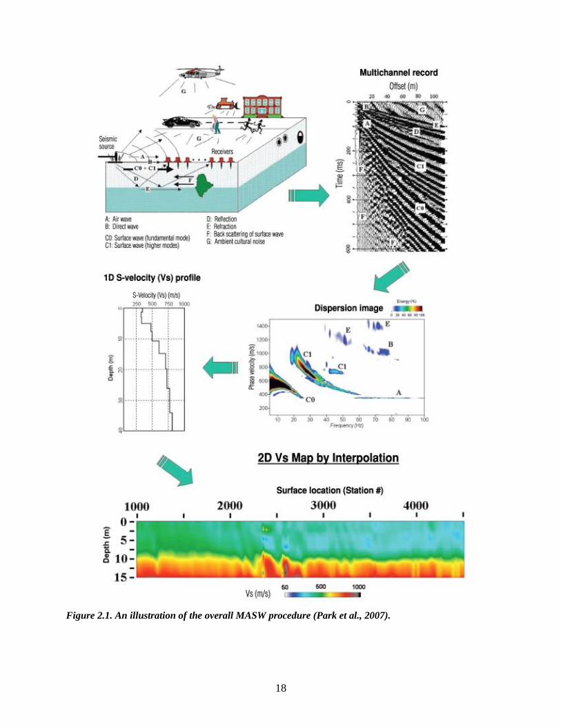
18

Figure 2.1. An illustration of the overall MASW procedure (Park et al., 2007).

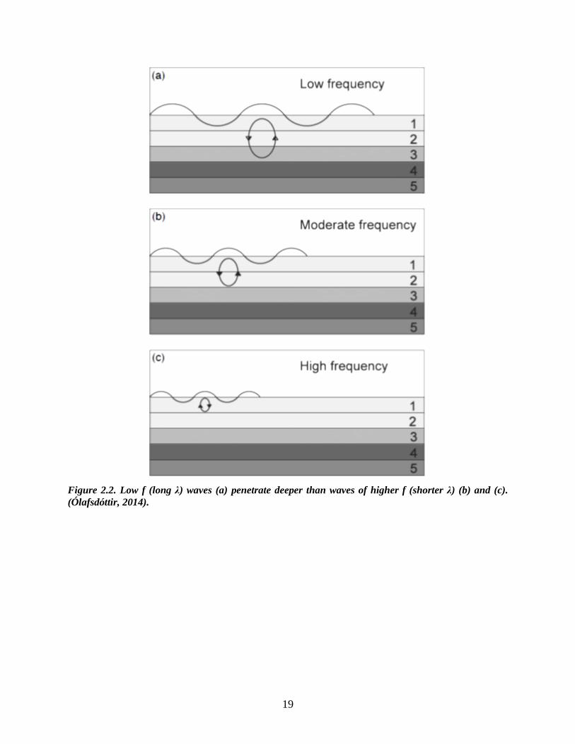
19

Figure 2.2. Low f (long λ) waves (a) penetrate deeper than waves of higher f (shorter λ) (b) and (c).

(Ólafsdóttir, 2014).

20

Figure 2.3. Flowchart and schematic of a typical local inversion algorithm (Olafsdottir, 2014).

21

(a) (b) (c)

Figure 2.4. Surface wave sources: (a) vertical source for Rayleigh waves; (b) angled wooden source for

Love waves; and (c) aluminum horizontal source for Love waves (Foti et al., 2017; Haines 2007).

Figure 2.5. Galperin source and traditional angled base plate (Hausler et al., 2018).

22

3. DATA COLLECTION AND PROCESSING

For this project, field testing was performed at Temple University’s Ambler campus by the

research team. The following sections present the selected field site, testing procedures, and data

post-processing used to generate results.

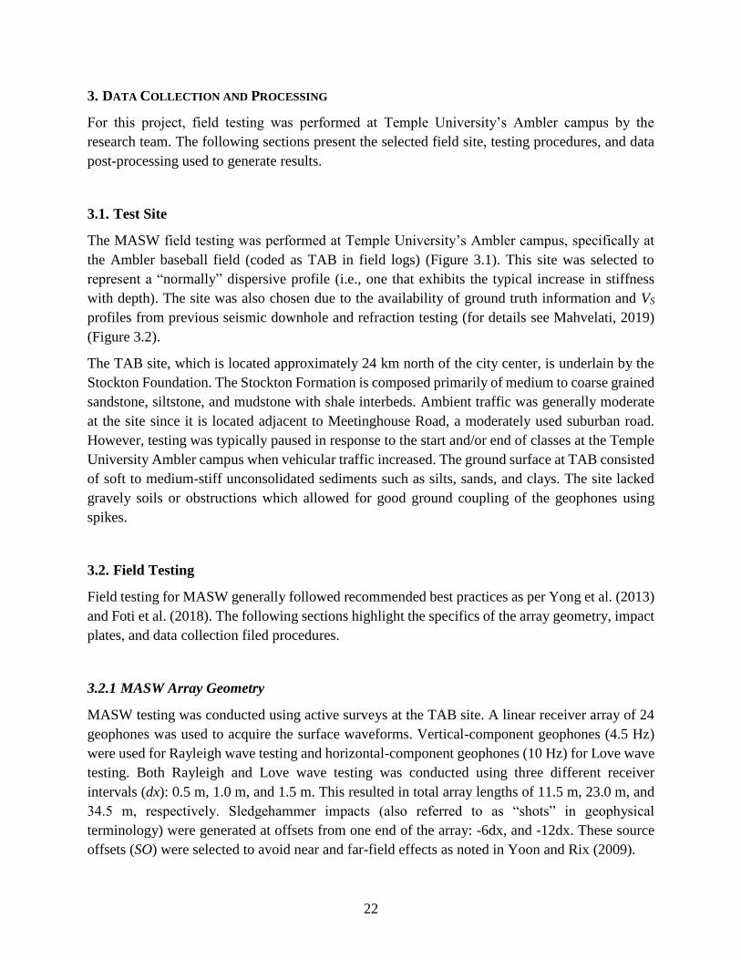
3.1. Test Site

The MASW field testing was performed at Temple University’s Ambler campus, specifically at

the Ambler baseball field (coded as TAB in field logs) (Figure 3.1). This site was selected to

represent a “normally” dispersive profile (i.e., one that exhibits the typical increase in stiffness

with depth). The site was also chosen due to the availability of ground truth information and VS

profiles from previous seismic downhole and refraction testing (for details see Mahvelati, 2019)

(Figure 3.2).

The TAB site, which is located approximately 24 km north of the city center, is underlain by the

Stockton Foundation. The Stockton Formation is composed primarily of medium to coarse grained

sandstone, siltstone, and mudstone with shale interbeds. Ambient traffic was generally moderate

at the site since it is located adjacent to Meetinghouse Road, a moderately used suburban road.

However, testing was typically paused in response to the start and/or end of classes at the Temple

University Ambler campus when vehicular traffic increased. The ground surface at TAB consisted

of soft to medium-stiff unconsolidated sediments such as silts, sands, and clays. The site lacked

gravely soils or obstructions which allowed for good ground coupling of the geophones using

spikes.

3.2. Field Testing

Field testing for MASW generally followed recommended best practices as per Yong et al. (2013)

and Foti et al. (2018). The following sections highlight the specifics of the array geometry, impact

plates, and data collection filed procedures.

3.2.1 MASW Array Geometry

MASW testing was conducted using active surveys at the TAB site. A linear receiver array of 24

geophones was used to acquire the surface waveforms. Vertical-component geophones (4.5 Hz)

were used for Rayleigh wave testing and horizontal-component geophones (10 Hz) for Love wave

testing. Both Rayleigh and Love wave testing was conducted using three different receiver

intervals (dx): 0.5 m, 1.0 m, and 1.5 m. This resulted in total array lengths of 11.5 m, 23.0 m, and

34.5 m, respectively. Sledgehammer impacts (also referred to as “shots” in geophysical

terminology) were generated at offsets from one end of the array: -6dx, and -12dx. These source

offsets (SO) were selected to avoid near and far-field effects as noted in Yoon and Rix (2009).

23

3.2.2 MASW Seismic Sources and Impact Plates

A 20 lb sledgehammer and a GISCO ESS-MINI accelerated weight drop (AWD) were used as

seismic sources in this study (Figure 3.3). Impacts were performed on sources angled at 0°, 15°,

30°, 45°, and 90° from vertical. The 20 lb sledgehammer was only used to perform the 90°impacts

since the AWD was incapable of that orientation. Variability in sledgehammer impacts was

reduced by using the same hammer operator, incorporating periods of rest to prevent fatigue, and

averaging the data from multiple hammer strikes. These efforts improved reproducibility and

ensured that the findings were statistically meaningful. These precautions were not needed when

using the AWD as the device is mechanical and produces consistent strikes. At each shot location,

multiple hammer strikes (typically 4) were stacked in order to increase the SNR of the recorded

waveforms.

The base plate used in MASRW testing was a 0.3 m x 0.3 m x 1.25 cm-thick aluminum plate. Three

different base plates were constructed for MASLW testing. Each base plate consisted of a 15 cm x

15 cm x 2.5 cm-thick aluminum plate over a wooden base which was cut at angles of 15°, 30°, and

45°. Figure 3.4 shows impact plates of 15°, 30°, and 45°. A 90° source was used for Love wave

testing that consisted of a 15.2 cm x 15.2 cm x 61 cm lumber post with galvanized caps on each

end. The vertical side of the plate was struck to produce horizontal ground motions.

3.2.3 MASW Data Collection

A Geometrics Geode seismograph and a field laptop with the Geometrics Seismodule Controller

Software (SCS) were used to acquire data. The surface waves were sampled at an interval of 0.125

ms for a total duration of 2.048 s (i.e. 16,384 samples). Initially, a trigger switch was attached to

the sledgehammer to begin data recording once impact was made on the baseplate. However, this

trigger proved inconsistent, so a geophone was planted adjacent to the baseplates as a triggering

mechanism for data collection

3.2.4 Additional Seismic Geophysical Testing

Previous to MASW testing at the TAB site, seismic refraction and downhole tests were also

performed to obtain ground truth information. Testing was performed at existing

boreholes/monitoring wells at the TAB site. The results from seismic refraction and downhole

tests were combined to generate a ground truth model of velocity (Figure 3.2) with which to

compare the results of the MASRLW testing. Details for this testing and analysis are provided in

Mahvelati (2019).

24

3.3. Data Processing

The data collected during these field investigations were post-processed using custom scripts in

the MATLAB computing environment, the Geometrics SeisImager/SW® software package, and

the Geopsy open-source seismic processing software package. The recorded signals were

evaluated for spectral content and relative energy using MATLAB. Subsequently, the dispersion

images (also referred to as overtone images) were generated in SeisImager/SW® which uses the

phase-shift method (Park et al., 1998) to convert the multichannel records in the time (t)-space (x)

domain into the frequency (f)-phase velocity (Cf) domain. Once fundamental mode dispersion

curves were selected from the overtone images, they were imported into the Geopsy software

package where a GSM neighborhood inversion algorithm (Wathelet, 2008) was implemented to

estimate the subsurface VS profile. Additional details about each of these steps is provided in the

following sections.

3.3.1 Spectral Content and Relative Energy

The acquired signals and corresponding dispersion images were examined for changes in energy

and spectral content. Spectral content was examined by generating the power spectra from the raw

signals using SeisImager/SW® and MATLAB. The shapes of the resulting power spectral density

(PSD) plots were compared using peak values, dominant frequency (fdom), and the shape factor (δ)

as a proxy for signal bandwidth (Vanmarcke 1976; Kramer, 1996):

𝛿 = √1 −𝜆1

2

𝜆0𝜆2 (Equation 3.1)

where λn is the nth spectral moment and can be computed as:

𝜆𝑛 = ∫ 𝐺(𝜔)𝜔𝑛𝑑𝜔𝜔𝑁

0

(Equation 3.2)

where ω is the angular frequency, ωN is the Nyquist angular frequency, and G(ω) represents the

PSD of the signal. Larger δ values correspond to larger signal bandwidths and δ always varies

between 0 and 1 (Kramer, 1996). Additionally, energy levels were evaluated based on the “relative

energy” concept introduced by Miller et al. (1986), where the summation of the squared Fourier

amplitude spectrum (i.e., power spectrum) provides an estimate of the energy generated by an

impact source and transferred into the underlying ground surface.

3.3.2 Signal to Noise Ratio (SNR)

SNR of the recorded waveforms were examined to evaluate the degree to which impact angle

negatively affect the raw signals. SNR represents the quality of collected waveforms and is defined

25

as the ratio of the signal power to the noise power. When the signal amplitude (AS) and noise

amplitude (AN) are measured, SNR can be calculated using:

𝑆𝑁𝑅 = 20 log10 (𝐴𝑆

𝐴𝑁) (Equation 3.3)

where SNR is expressed in units of decibels (dB). In this study, SNR was determined for a given

trace by comparing the maximum amplitude of the coherent signal within a shot window to a

representative noise level recorded at the site of interest. In other words, all the maximum

amplitudes extracted from the waveforms were divided by a constant amplitude representing the

average noise threshold at the site. This representative noise level was estimated at each site based

on data from several acquisitions at different offsets. The maximum amplitude of signals picked

from the latter part of the recording duration (i.e., after the primary shot signal has completely

propagated through the receiver array) were subsequently selected and averaged. The reason for

this approach is that different records were influenced by different amounts and sources of

background noise. Even though caution was used during field testing to collect data when

background noise was minimized, these noise levels still fluctuated and could systematically bias

the estimates of SNR if each trace were normalized by its own level of background noise.

3.3.3 Dispersion Information

For this research effort, the overtone images from MASW testing were used in two ways. First,

they were examined to extract a fundamental mode dispersion curve for the site. To extract this

curve, suggested points from the automatic algorithm embedded in the SeisImager/SW® software

were cross-examined with theoretical dispersion curves computed for the ground truth model at

the TAB site. The curve selection process was repeated for all the shot records of interest and

multiple dispersion curves were extracted. Then, select subsets of dispersion curves were averaged

together to create representative dispersion curves as described in Olafsdottir et al. (2018). The

dispersion curve data points from Rayleigh and Love waves, regardless of their offset, source, or

interval, were averaged and examined in a single figure. This process allowed for direct

comparison of MASRW and MASLW dispersion curves. Next, the dispersion curves were analyzed

based on an average according to base plate angle.

The overtone images were also evaluated directly and compared with each other by taking their

difference. This allowed a review of the following issues: energy partitioning between the

fundamental and higher modes, low-frequency fundamental-mode performance, high-frequency

fundamental-mode performance, and uncertainty in fundamental mode dispersion curve

interpretation.

26

3.3.4 Inversion

The dispersion curves generated in the previous step of data post-processing were used in the GSM

implemented within the Geopsy software package to perform both independent inversion of

Rayleigh and Love waves and joint inversion. This GSM uses an improved neighborhood

algorithm developed by Wathelet (2008). Rather than starting from an initial “guess” of the

subsurface VS as in a local search method, this GSM defines a probability density distribution for

each model parameter (i.e., VS, VP, ρ, t). This parameterization creates a range of potential models

over which the global algorithm searches for the best model, using a randomly generated seed

model for the starting point (Foti et al., 2017). This seed model is iteratively adjusted to identify

the best model whose forward response fits the experimental dispersion information (obtained in

the previous step).

The control parameters implemented in the neighborhood algorithm within Geopsy include: (1)

the number of models chosen at random inside the parameter space at the beginning of the

inversion (NS0); (2) the number of models to generate at each iteration (NS); and (3) the number

of best cells (with the lowest misfit) where the NS models are generated (NR). Selection of an

appropriate parameterization must balance the need to explore a wide range of potential models

with computation expense and the extent to which most models represent unrealistic subsurface

conditions for the site of interest (Cox and Teague 2016). The inversion is more exploratory if the

NS new samples are distributed on many cells (i.e., NR is high). The inversion is more restrictive

if it optimizes more by limiting the NS new samples to the very few best cells (i.e, NR is low).

Wathelet (2005) notes that generally better misfits are obtained with fewer iterations if NR is low,

but the inversion is more trapped in local minima. Consequently, larger values for NR and NS can

provide better final misfits at the expense of greater number of iterations and the associated

computational costs.

For this study, the model was parameterized using the following criteria:

• P-wave Velocity (VP): 6 layers (5 plus a halfspace) limited to VP between 200 m/s to 8000

m/s. Bottom of layer was linked to the bottom of the layers defined for VS.

• S-wave Velocity (VS): 6 layers (5 plus a halfspace) limited to VS between 150 m/s to 4000

m/s.

• Density (ρ): Single layer with fixed 2000 kg/m3 value.

• Poisson’s Ratio (ν): Single layer limited between 0.2 to 0.5.

• Inversion Tuning Parameters: NS0 = 100; NS = 50000; NR = 100.

In order to evaluate the effectiveness of the inversion, a misfit function is defined, which represents

how close an experimental dispersion curve is to the measured dispersion curve during the

subsequent forward modeling. For this study, based on the information input into the inversion

algorithm, this misfit function simplifies into a root-mean-square error (RMSE):

27

𝑅𝑀𝑆𝐸 = √(1

𝑁) ∑(𝐶𝑖

𝑇 − 𝐶𝑖𝑀)2

𝑁

𝑖=1

(Equation 3.4)

where CiT and CM

i are the phase velocity at the ith frequency component for the theoretical and

measured dispersion curves, and N is the total number of data points. VS models were selected

based on the lowest RMSE misfit within a tolerance of +1%. This allowed for some measure of

the uncertainty involved in the global inversion process.

28

Figure 3.1. Temple Ambler campus site and survey line (Google Earth).

(a) (b)

Figure 3.2. Ground truth model at TAB: (a) VS and VP profile; and (b) Rayleigh and Love wave

dispersion curves (Mahvelati, 2019).

0

10

20

30

40

50

60

70

80

90

100

0 500 1000 1500

Freq

uen

cy

(H

z)

Phase Velocity (m/s)

Love, M0 Love, M1

Love, M2 Rayleigh, M0

Rayleigh, M1 Rayleigh, M2

29

Figure 3.3. AWD positioned at impact angles of 15°, 30°, and 45° (Mahvelati, 2019).

Figure 3.4. Custom impact sources for 15°, 30°, and 45° (Mahvelati, 2019).

30

4. ANALYSIS OF RESULTS AND DISCUSSION

In order to understand the effect of base plate angle on the simultaneous generation of Rayleigh

and Love waves, the frequency (f) content, relative energy, and signal-to-noise ratio (SNR) of the

waveforms were examined. Shear wave velocity (VS) profiles were also generated through

independent and joint inversion of the acquired Rayleigh and Love waveforms. These results were

generated for all testing performed at the site with both an accelerated weight drop (AWD) and 20

lb sledgehammer source and multiple source offsets (SO = -6dx and -12dx), receiver spacings (dx

= 0.5 m, 1.0 m, and 1.5 m), and impact angles (0°, 15°, 30°, 45°, and 90°) as described in Chapter

3. The multiple SO and dx were used to ensure repeatability of the trends exhibited across impact

angles. The results presented herein were developed in service of answering the following two

research questions:

1. What is the optimal angle of impact for simultaneous generation of Rayleigh and Love

wave generation?

2. How effective are vertical impacts for generating simultaneous Rayleigh and Love waves?

The following sections highlight the major findings of this study with respect to these research

questions.

4.1. Frequency Content

The f present in a surface wave is an important parameter to ensure adequate coverage for

development of a dispersion curve during MASW analysis. It was anticipated that changes to the

impact angle would result in different performance with respect to f. For example, certain

frequency bands may be more emphasized than others as the impact angle was varied from vertical

to horizontal. This was initially examined by transforming the time-domain waveform signals into

the f domain. The Fourier transform of a signal breaks down the entire signal into individual f

components. The power spectrum [or power spectral density (PSD)], which similarly examines

the relative power contribution of each f component, is computed by squaring the magnitude of a

signal’s Fourier amplitude spectrum, normalized by the number of f samples.

Figures 4.1 and 4.2 plot the normalized PSD of the collected waveforms as a function of f for the

different SO, dx, and impact angles. Each sub-figure was normalized to the largest peak PSD

within the plotted dataset. For Rayleigh wave data, the 90° orientation was not collected during

field testing. A higher PSD indicates that a particular f component was more prevalent in the

acquired waveform data, which should generally improve recognition of its corresponding phase

velocity within the dispersion image. Therefore, the relative differences between curves in each

sub-figure indicate how much the impact angle improved or degraded the power contributions of

a particular f range and its presence in the corresponding dispersion image. Consequently, these

normalized PSD plots were analyzed to examine differences in their relative shape and peak PSD

values.

31

4.1.1 Rayleigh Waves

The Rayleigh wave power spectra remained generally consistent when observed across the various

SO and dx used in this study. One of the first observations that can be made when comparing the

normalized PSD plots is the relationship between impact angle and peak PSD. Impact angles of 0°

and 15° produced the largest peak PSD values, while a 45° impact typically had the lowest peak

values no matter the SO or dx. An outlier in this trend occurred at the -6dx and 0.5 m spacing,

where the 45° impact produced a peak PSD value comparable to the other impact angles. The

vertical polarization of Rayleigh waves explains the lower peak PSD values for the 45° impacts,

which was 0.60 when averaged among the three offsets. This is a significant reduction compared

to the 0° and 15° impacts (i.e., a 65.7% difference and a 58.8% difference, respectively).

When the peak normalized PSD values were averaged over both the -6dx and -12dx offsets, the 0°

impact again produced the largest peak normalized PSD as would be expected for Rayleigh wave

generation that tends to favor vertical strikes (i.e., 0° impacts). However, the average difference

between the peak power of the 0° and 15° impacts (across all SO and dx) was less than 4.5%.

Likewise, the difference between 15° and 30° impacts when averaged across SO and dx was

approximately 10%. This implies that impacts at slightly less than vertical can still generate

significant power in the dominant f band of the propagating wave. Moreover, the Rayleigh wave

PSD seem to exhibit less overall sensitivity and scatter with respect to the impact angle. The switch

from a 30° impact to a 45° impact proves to be the most detrimental to peak PSD based on the

results of Figure 4.1.

Changes in impact angle may have a significant impact on the overall shape of the PSD plot, which

can manifest as shifts in the dominant f present in a waveform and the overall bandwidth.

Therefore, dominant frequency (fdom) and signal bandwidth are also important factors to consider

for frequency content analysis. The fdom is the frequency that carries the most energy in the

spectrum. Bandwidth is the difference between the upper and lower frequency in a continuous

band of frequencies. It is typically found by examining the PSD plot and determining the first and

last frequency associated with a power spectral density equal to half the peak value (Kramer 1996).

However, this definition causes the measured bandwidth to be highly affected by localized

variations in the amplitude of the power spectra. In this study the shape factor (δ) as defined by

Vanmarcke (1976) was used as a measurement of signal bandwidth as noted in Chapter 3.

Based on the results in Figure 4.1, the fdom for the 0° impact was generally the highest of all the

impacts, regardless of the source offset and receiver spacing (Table 4.1). This implies that by

angling the impact away from vertical, the peak PSD values shift to lower frequencies. However,

these changes were a rather small effect. On average, the difference between maximum fdom (0°

impact) and minimum fdom (typically 45° impact) was 7.7%. The results for δ pointed towards an

overall increase in bandwidth as the angle was shifted away from 0° towards more horizontal

(Table 3.2). For example, δ increased on average by more than 4.5% at 15°, 30°, and 45° impact

angles when compared to 0° impacts. This implies that the shift in the fdom towards lower

32

frequencies at more horizontal impacts was also accompanied by an overall broader shape for the

PSD plot. Consequently, although the peak PSD value decreased with the 15°, 30°, and 45°

impacts as a result of the energy partitioning into both vertical and horizontal components, there

was an overall shift towards increased participation from a broader range of frequency bands.

4.1.2 Love Waves

The Love waveforms were analyzed in the same manner as the Rayleigh waveforms. For Love

wave generation, the purely horizontal (90°) impact actually proved to generate the smallest peak

normalized PSD value. This was related to the seismic source used for the 90° impact (20 lb

sledgehammer), which generates substantially less energy than an AWD. The 0° impact generated

the second lowest peak normalized PSD. This result also makes sense given that a purely vertical

impact will primarily generate vertically-polarized wave energy. Nevertheless, an examination of

Figure 4.2 highlights that even a purely vertical impact will generate normalized power spectra

within approximately one half the peak normalized PSD from more favorable impact orientations.

Moreover, use of an AWD will allow this 0° impact to compare with a purely horizontal (90°)

impact with a much smaller 20 lb sledgehammer seismic source.

The effectiveness of generating both Rayleigh and Love waves with a purely vertical strike (i.e.

0°) was also examined with regard to PSD. As was expected, the 0° impact produced the highest

average peak PSD values for Rayleigh waves. However, for Love waves the 0° impact performed

second worst, behind the 90° impact which used the significantly less powerful sledgehammer

source. For Love waves, the 0° impact produced an average peak PSD value of 0.62 when averaged

across all SO and dx. This value was within approximately 40% of the highest average peak PSD

value. Consequently, although a 0° impact will produce significantly less powerful Love waves

compared to an ideal strike, it may still be able to generate usable data for MASLW analysis.

Additional examination of the PSD in Figure 4.2 highlights that the 30° impacts unexpectedly

generated the largest peak normalized PSD values in nearly every case. The 15° impact angle

generated the highest peak normalized PSD for the closest source offset and receiver spacing and

was generally within a few percentage points of the 30° impact angle. Consequently, when the

peak normalized PSD values were averaged across the different offsets and receiver spacings, the

15° impact angle actually performed best for Love wave generation, with the 30° impact angle on

average exhibiting only a 1.5% smaller peak normalized PSD. These results suggest that Love

wave generation was more robust at less than optimal impact angles (i.e., 0°, 15°, and 30°).

The 45° angle of impact did not perform as well as predicted for Love wave generation in terms

of peak power. These results are somewhat surprising, as Love waves tend to favor more horizontal

impacts and the 45° impact had the largest horizontal component in the impact force vector

compared to the flatter angles of 15° and 30°. The lower-than-expected PSD for the 45° impact

may have been due to issues with ground coupling and/or general wear and damage to the source

as testing progressed. For example, as the impact angle approached closer to horizontal with such

33

a large AWD source, the larger horizontal component of the impact force vector may have caused

the base plate to slide along the top of the ground surface. More intermediate angles, such as 15°

and 30°, contained enough vertical force during impact to “wedge” the base plate in place and

actually couple the horizontal wave energy to the ground better.

As with the Rayleigh wave results, the Love wave PSD were examined for changes in shape and

fdom. The average fdom varied similarly with impact angle compared to Rayleigh waves. As with the

Rayleigh wave results, the shift away from the “ideal” impact angle (in this case from 90° towards

more vertical impacts) led to an average decrease in the predominant frequency of similar

magnitudes (Table 3.3). However, the trend was practically (though not technically) reversed for

Love wave impacts relative to Rayleigh waves with respect to the bandwidth proxy selected for

this study (i.e., δ). The Love wave PSD exhibited an increase in δ as the impact angle increased

from completely vertical (0°). However, a completely vertical impact is the least optimal

orientation for the seismic source when trying to generate horizontally-polarized Love waves.

Consequently, when viewed as a trend from most favorable angle for Love wave generation (90°)

to least favorable (0°), the δ tended to decrease, which implies a narrower bandwidth. This signifies

that less than optimal impact angles for Love waves tend to “focus” their energy into a narrower

frequency band shifted towards lower frequencies. The corresponding “loss” of high-frequency

content may negatively impact the predictions of the VS structure in the immediate near surface

(e.g., upper 1 m to 2 m).

4.2. Relative Energy

It should be noted that peak normalized PSD does not directly measure the total wave energy,

which is based on the entire waveform rather than a single “spike” in the PSD plot. Therefore, a

more comprehensive parameter must also be examined to better analyze the effect of impact angle

on the energy transferred into the subsurface. The summation of the squared Fourier amplitude

spectrum (i.e. power spectrum) provides an estimate of the “relative energy” generated by an

impact source based on the efforts of Miller et al. (1986).

Typically, higher relative energy translates to larger SNR and clearer dispersion curves, which can

improve the accuracy of VS profiles. Relative energy levels were examined as a function of impact

angle to analyze how well a particular orientation transferred impact energy into the subsurface.

The results of the relative energy analysis should compare favorably to the conclusions drawn from

the peak normalized PSD analysis, though there may be some subtle difference introduced by the

scale of the two parameters. Figures 4.3 and 4.4 plot the normalized relative energy as a function

of array configuration (i.e. impact angle, SO, dx, and wave type). In each sub-figure, a normalized

relative energy level of 1.0 indicates the highest energy when compared to the rest of the

configurations.

34


The Rayleigh wave relative energy results in Figure 4.3 reinforced many of the same trends noted

in the PSD results in Figure 4.1. For example, the 0°, 15°, and 30° impacts produced similar

relative energy levels for both the -6dx and -12dx offsets. Generally, the 15° impact produced the

highest average relative energy over the three dx values (1.5 m, 1.0 m, and 0.5 m) and both SO (-

6dx and -12dx). At -12dx, the 0° impact produced the highest average energy over the receiver

spacings. When the relative energy from -6dx and -12dx were averaged together, the 15° impact

produced the highest normalized energy. However, the difference between normalized energy

from the 0° and 15° impacts was just 1.6%. The weakest impacts for Rayleigh waves occurred at

the 45° impact angle. At -6dx, the average relative energy for a 45° impact was 0.65. At -12dx, the

average relative energy for a 45° impact was 0.48. The energy generated by a 45° impact for

Rayleigh waves was 53.8% lower than a 15° impact. These results align well with the previous

analysis of the PSD that seemed to point to modest sensitivity of impact angle for Rayleigh waves

until an angle of 45° is reached.

4.2.2 Love Waves

For Love waves, the 30° impact produced the highest relative energy over both the -6dx and the -

12dx offsets. The second-best impact angle for Love wave generation was 15° based on the

normalized relative energy values. The difference between the energy generated by the 15° and

30° impacts was 11.8%, indicating that relatively vertical impacts can generate useful Love wave

energy. As with the Rayleigh wave data, these results corroborate the PSD analysis based on peak

values. However, there were some minor discrepancies. For example, the 45° impact at -6dx

performed better in terms of normalized relative energy when compared to the normalized PSD.

For the 1.5 m and 0.5 m dx values, the 45° impact produced a normalized relative energy of 0.92

and 1.0, respectively. However, the average relative energy at -6dx was again reduced by a

significant outlier at the 1.0 m spacing.

The 90° impact generated the least energy due to the reduced power of the 20-lb sledgehammer

compared to the AWD. The 0° impact performed second worst in terms of relative energy. To

examine the effectiveness of generating both Rayleigh and Love waves using a vertical impact,

the energy generated by a vertical strike was compared to the energy generated at an ideal angle.

As was predicted and shown in the PSD analysis, the energy generated by a 0° strike was much

lower for Love waves. The 0° strike generated 56.8% less energy than the most powerful strike.

Nevertheless, the 0° impact results in Figure 4.4 indicate that a purely vertical impact with an

AWD is capable of transferring as much energy into the ground as a 20 lb sledgehammer impacting

a base plate at the most ideal angle (90°).

The 15° impact produced the highest normalized energy for Rayleigh waves over both the -6dx

and -12dx offset. However, this average normalized energy was only 1.6% greater than the energy

generated by a 0° impact. For Love waves, the 30° impact produced the greatest normalized energy

35

over both offsets. The 30° impact produced, on average, 11.8% more energy than the second-best

impact angle, which was a 15° impact. The 30° impact also produced strong Rayleigh waves; the

30° impact was just 4.8% less powerful than the optimal 15° impact for Rayleigh waves. Therefore,

based on relative energy, it appears that the 15° and 30° impacts produce similar results for the

simultaneous generation of Rayleigh and Love waves. It should be noted, however, that higher

relative energies do not necessarily translate to more clear and accurate dispersion images. While

the 90° impact did not produce large peak energy for Love waves, the shape of the power spectra

compared favorably indicating sufficient f coverage for the development of a useable dispersion

image.

4.3. Signal-to-Noise Ratio (SNR)

As noted in Chapter 3, SNR was determined for the acquired waveforms by comparing the

maximum amplitude of the coherent signal to a representative noise level (i.e. the average noise

threshold at the site). The purpose of this analysis was to determine if differences in relative energy

led to changes in SNR. Figures 4.5 and 4.6 plot SNR as a function of channel number along the

receiver array, where the channel numbers increase with distance away from the source.


The plots of SNR for Rayleigh waves show that the SNR of the 45° impact was consistently the

lowest out of the four impact angles. The highest SNR for Rayleigh waves was at the 15° impact,

both for -6dx and -12dx. These results mirrored the observations in the PSD and relative energy

analyses. When averaged across the all channels, the SNR value for a 15° impact was 9.8% larger

than the SNR for the 45° impact. At distances closer to the source, the SNR ratio for the 45° impact

was closest to the SNR of the other impact angles. The difference in SNR was exacerbated by

increasing distance from the source. This trend indicates that for Rayleigh waves, the effect of

impact angle on SNR becomes more apparent at greater distances. Note, for example, in Figure 4.5

how many of the SNR curves diverge more at the farther channels of the arrays. For dx of 1.5 m

and 1.0 m, the SNR trend decreased with distance from the source. However, for dx of 0.5 m, the

SNR increased with distance from the source. This discrepancy is likely due to the fact that the

array length for dx = 0.5 m is short, at 12 m. Near-field effects may have degraded the SNR at the

closer receivers.

4.3.2 Love Waves

The Love wave SNR was lowest for the 45° and 90° impacts, which was expected based on the

previous results for f and relative energy. The SNR for the 90° impact was 7.1% lower than the

highest average SNR, which was at the 30° angle. The lower-than-expected SNR for the 90° impact

is caused by the smaller impact source used for testing at that angle. The 20-lb sledgehammer

36

generated significantly less power than the AWD, and less power generally equates to a lower

SNR. As explained previously for the PSD and relative energy results, the low SNR for the 45°

impacts may be attributed to issues with coupling between the impact source and base plate. This

in turn can be attributed to two main sources: (1) relative slippage between the base plate and the

ground surface; and (2) wear and damage of the base plate.

When the SNR for Love waves were averaged, both for -6dx, -12dx, and overall, the highest SNR

occurred for the 30° impacts. The SNR at 30° was 7.5% higher than the lowest overall SNR, which

was at 45°. Consequently, this optimal angle for SNR is lower than a hypothesized optimal angle

of 45°.

Based on the percent differences between the maximum and minimum SNR values for both

Rayleigh and Love waves, it appears that Love wave SNR is less affected by impact angle than

Rayleigh waves. Nevertheless, the differences in minimum and maximum SNR were small. The

optimal impact angle for generating the highest SNR was 15° for Rayleigh waves and 30° for Love

waves. However, it should be noted that a higher SNR does not always translate to a higher quality

dispersion image as discussed in the next section.

4.4. Effects on Dispersion Information

The dispersion curve is a critical component of the MASW procedure, so the effect of base plate

angle on dispersion information should be examined. Though qualitative in nature, an analysis of

the quality of the dispersion image can highlight any potential improvements in survey resolution

and depth of investigation based on the potential to extract an accurate dispersion image over a

wide f range. Figures 4.7 and 4.8 present the differences between overtone images generated by

various impact angles at different offsets and dx. Each dispersion image was compared to the

“optimal” dispersion image (replicated as the top sub-figure) based on impact angle (i.e. 0° for

Rayleigh and 90° for Love). The blue and red color scheme represents a negative or positive

difference in normalized amplitude, respectively. If more information is available from the optimal

dispersion curve (i.e. 0 or 90°), red is present; if more information is available from the compared

dispersion curve, blue is present.


For Rayleigh waves, the 0° impact produced the best dispersion curves in terms of clarity and

fundamental mode identification. This conclusion follows the results of the PSD, relative energy,

and SNR analysis, where a 0° and 15° impact generated the most power, transferred the most

energy, and exhibited the best SNR. However, the quality of the Rayleigh wave dispersion curves

was generally poor, even for the 0° impact angle. It was often difficult to identify an obvious and

continuous fundamental mode dispersion curve in the overtone images even at an optimal impact

37

angle. This suggests that the TAB site exhibits a pattern of modal excitation that causes modal-

mixing during surface wave propagation. Moreover, the use of angled impacts tended to intensify

this effect. For example, the blue sections of the bottom sub-figures along the areas where a

fundamental mode can be extracted indicate decreased normalized amplitude (i.e., decreased

fundamental-mode participation during surface wave propagation). This indicates that the effect

of an increase in impact angle from vertical is higher modal participation in the overtone image

and more difficulty in selecting a fundamental-mode dispersion curve. There was generally little

difference between the -6dx and -12dx offsets for Rayleigh wave overtone images. However, the

1.0 m receiver spacing tended to produce clearer dispersion curves, particularly at higher

frequencies.

The 15° impact generally compared favorably to the 0° impact overtone images, particularly in the

upper frequency range. The largest differences occurred below approximately 35 Hz. This trend

may be due to noise that manifests as error during the phase-shift method. At the lowest end of the

frequency range, the coherent signal competes with noise, which when processed into the overtone

image yields incoherent amplitude information and large scatter in the dispersion information.

Fundamental-mode identification suffered somewhat, but otherwise compared favorably between

the 0° and 15° impacts above this frequency. The 30° impact also produced reasonably clear

dispersion curves comparable to the 15° impacts. This is not completely surprising considering the

energy generated by the 30° impact and the reasonably high SNR.

4.4.2 Love Waves

The 90° impact produced the clearest dispersion curves for Love waves. This outcome is expected

given what is known about ideal Love wave generation but does not follow the trend of the power

and SNR analysis. The fact that a 90° impact with a 20-lb sledgehammer could produce

significantly less energy than other impacts and yet still generate the clearest overtone images

shows that power does not necessarily equate to a quality dispersion curve. The 90° impact

produced a strong fundamental mode over a wide range of frequencies.

Overall, the quality of the Love wave overtone images was excellent, and the fundamental-mode

for Love wave propagation was significantly easier to identify than for the Rayleigh wave

overtones. This indicates that the TAB site is one where Love wave propagation is less complex

and less subject to significant modal-mixing. Arrays with the various dx produced dispersion

curves of similar quality. However, higher modes became clearer as dx was increased. In general,

higher modes were easier to identify through Love wave dispersion images than Rayleigh wave

dispersion images.

In line with the conclusions drawn from the power and SNR analysis, the 45° and 30° impacts

again performed well. Despite lower energy and SNR, the 45° impact performed second-best after

the 90° impact. The largest differences in the overtone images for these impact angles and the 90°

impact occurred at very low and very high f. As with the Rayleigh wave overtone images, this

38

discrepancy may be a result of noise manifesting as error. Despite the differences at high and low

frequencies, a fundamental mode could still be identified that compared favorably to the optimal

dispersion curve. Interestingly the 15° and 0° impacts also produced dispersion curves from which

a similar fundamental mode could be identified, although there was significantly more variation

throughout the entire overtone image for each of these impact angles.

For each impact angle, differences between the 90° and other overtones became apparent in the

40-60 Hz range. In this range, the overtone images of other impact angles performed worse in

terms of fundamental-mode identification. The discrepancy became more distinct as the impact

angle moved closer to 0°. While the differences between the 0° and the 90° overtone images were

obvious, reasonably accurate dispersion curves were still able to be obtained from the 0° overtone

images (Figure 4.9). Both fundamental and higher modes could be picked from the dispersion

image. This result indicates that vertical strikes may be reasonably effective for generating Love

waves, which could significantly improve acquisition times and increase the accuracy of the final

VS profile.

4.5. Shear Wave Velocity (VS) Profiles

A series of VS profiles was generated for both Rayleigh and Love wave data using the improved

neighborhood inversion algorithm proposed by Wathelet (2008) and implemented in the Geopsy

software package. The inversion was performed independently as well as jointly, for a total of

three subsurface VS profile estimates. The inversion parameterization was described in Chapter 3.

Figures 4.10a – 4.12a show VS profiles for each impact angle of the Rayleigh and Love wave data

collection. The solid line of each VS profile represents the solution that best fits the dispersion

curve obtained from field data. The dashed lines on either side of the solid line represent the

uncertainty for the best fit solution. These dashed lines indicate comparable VS profiles within a

pre-specified limit of uncertainty (i.e., within 1% of the lowest misfit value). Dashed lines that are

very close to the solid line would indicate that there is little velocity variability and/or uncertainty

within those limits.

Figures 4.10b – 4.12b also present the associated misfit between the predicted VS and the ground

truth VS (i.e., Equation 3.4 applied to differences between predicted VS values instead of dispersion

curves). These plots reflect how difference there is between the inverted and ground truth VS

estimates as a function of depth. A lower RMSE misfit indicates less error and vice-versa.

Additionally, the rate of change in the RMSE plot indicates whether the velocity layer at that depth

is improving the overall prediction or adding to the error. For example, when the RMSE decreases

with depth, the inverted VS profile is more accurately predicting the ground truth VS. The

intersection points with the x-axis in Figures 4.10b – 4.12b represents the global overall RMSE

for the VS profile (i.e. how accurate the entire profile is on average across the entire depth). For

this research effort, seismic refraction and downhole testing were used to obtain ground truth

information at the TAB site.

39


For Rayleigh waves, the inverted VS profile generated by all impacts were practically identical for

the upper 1.5 m of the site and exhibited the same RMSE between the predicted VS and ground

truth VS. Beyond that depth the 45° results start to perform the worst compared to the other impact

angles, though the difference is relatively modest. However, even the better-fitting VS profiles

varied significantly from the ground truth model through most of the profile, highlighting the

issues faced at this site with MASRW.

While each impact angle performed similarly up to a depth of approximately 5 m, the 45° impact

compared most favorably to the ground truth model at depths greater than 7 m. Because the 45°

impact performed better at depth, it should be considered the best VS profile compared to the

ground truth model. This is indicated by the lowest overall RMSE between the 45° impact inverted

model and ground truth. In fact, the global RMSE for the 45° impact angle when computed across

all depths is approximately half the next smallest RMSE (0° impact).

Rayleigh wave VS profiles had significant uncertainty (i.e. space between the dashed lines) at

deeper strata. Uncertainty tended to increase as the impact angle approached horizontal. By far,

the most uncertainty in the inverted VS profile corresponded to the 45° impact. However, even the

0° impact angle suffered increased uncertainty at depth. It should be noted that although the 45°

VS profile appears to be close to the ground truth profile at depths greater than 7 m, the very high

uncertainty of the 45° inversion prevents it from being considered an accurate VS profile. The 30°

impact actually appears to have the lowest VS uncertainty at depth. This result may be due to the

source orientation or stronger source-ground coupling that allowed more energy from the AWD

impact to be generated into the subsurface. Consequently, when considering both RMSE and

amount of uncertainty present in the inverted VS profile, the superior Rayleigh inversion model

appears to be the one generated from waveforms generated by a 0° impact (as would theoretically

be expected).

Higher uncertainty at deeper strata can be explained by a lack of low-frequency energy in the

surface wave. Lower f are required to accurately image deep strata, so if an impact angle is not

able to generate f in such a range, the uncertainty at depth increases. This uncertainty is manifest

in the VS profile as a wider range of potentially viable inversion models. Greater uncertainty as the

impact angle approached 45° indicates moving the impact angle towards horizontal negatively

impacts low-frequency generation for Rayleigh waves. This appears to contradict the PSD results

that pointed to a shift in low frequency response as the angle was made more horizontal. However,

an examination of the relative energy quickly highlights that, though the predominant frequency

may have shifted to a lower value/range, the overall energy transferred into the subsurface was

drastically reduced for the 45° impact. This can consequently explain the increased inversion

uncertainty at depth relative to the other impact angles.

40

4.5.2 Love Waves

In general, VS profiles generated from Love wave data compared more favorably to the ground

truth model than Rayleigh wave profiles. This was evident based on the lower overall RMSE

values when taking the entire depth profile into account as well as the reduced inversion

uncertainty present in the results of Figure 4.11. At the near surface (i.e. less than 3 m) Rayleigh

wave VS profiles tended to match ground truth information better than Love wave profiles.

However, at intermediate depth (i.e. between 4 and 10 m), Love wave profiles showed

improvements over Rayleigh profiles.

For Love waves, the 90° and 45° impacts generated the best-fit profiles. These impact angles also

had the lowest uncertainty. While the 90° and 45° impacts performed best compared to the ground

truth model, the other three impact angles produced reasonably similar VS profiles. There was no

significant difference between the impact angles at depths less than 3.5 m, but uncertainty in the

inversion results increased as the impact angle approached vertical. This inversion uncertainty was

notably less than uncertainty in the Rayleigh wave inversion, even for the worst-performing impact

angles (i.e. 0° and 15°). As with the Rayleigh wave profiles, the trend of increased uncertainty

with depth can be explained by a lack of low-frequency waves necessary to accurately image

deeper strata. The accuracy of the Love wave VS profiles may have been improved by using a more

powerful strike for the 90° impacts and improving the ground coupling and durability of the 45°

source.

For Love waves, the 30° impact performed reasonably well. At depths greater than 8 m, the 30°

impact performed very similarly to the 45 and 90° impacts. The most notable difference between

the 30° impact and the more horizontal impacts occurred at 5 m where the 30° angle underpredicted

VS. Uncertainty in the 30° inversion was also similar to the 90° and 45° inversions, although

uncertainty increased at depths greater than 10 m. Although the 0° and 15° impacts performed

moderately well at depths up to approximately 5 m, uncertainty increased significantly at greater

depths. Still, the Love wave VS profiles seemed to be less dependent on impact angle than Rayleigh

waves with less overall scatter between the VS predictions from different impact angles.

Consequently, selection of an optimal impact angle may be able to be guided more explicitly by

Rayleigh wave generation at this site given the sensitivity to impact angle and poor overall

performance of Rayleigh waves due to modal-mixing and higher-mode participation.

4.5.3 Joint Inversion

Joint inversion of Rayleigh and Love waves was also performed to elucidate any further constraints

on selection of the optimal impact angle. Figure 4.12 shows the results of joint inversion. Joint

inversion seemed to improve the accuracy of VS profiles relative to the ground truth model by

combining the Rayleigh wave accuracy at shallow and deep layers with the Love wave accuracy

at intermediate-depth layers. During joint inversion, uncertainty was likely reduced by the

additional constraints introduced by utilizing both Rayleigh and Love wave data. Furthermore, the

41

joint inversion may have benefited from the higher-quality data offered by Love waves. In

particular, joint inversion appears to have significantly less uncertainty as depth increased. Joint

inversion also more closely aligned the VS profiles of each impact angle, resulting in less overall

scatter between the profiles. For example, while there were significant differences between the 0°

and 45° Rayleigh wave profiles, the VS profiles of these two impact angles performed similarly

after joint inversion. After joint inversion, the 30° profile appears to have the best fit and lowest

uncertainty though this profile was still appreciably different than the ground truth model.

4.5.4 Comparisons Between Inversion Results

The large differences between the MASW and ground truth VS profiles for both Rayleigh and Love

waves can potentially be explained by inherent differences in the seismic geophysical testing

procedures used at the TAB site. While the boreholes used for downhole testing were close to the

MASW site, they were not in the exact location. The subsurface may experience significant

changes over a relatively small area. These differences could explain discrepancies between the

inverted VS profiles and ground truth. Likewise, the seismic refraction results were converted into

a 1-dimensional VS profile from a 2-dimenstional profile.

Compared to Rayleigh waves, Love waves performed slightly worse at the immediate near surface

(i.e. above 1 m). Love waves performed better than Rayleigh waves for approximately 4 m through

11 m. In this range, the RMSE error was less for Love waves although the variability between

impact angles was greater. The Love wave profiles exhibit slightly better RMSE at greater depths,

but the 0° and 15° results were comparable to Rayleigh waves. For Love waves, the 90° impact

performed best overall (with 45° not far behind), while the 15° impact displayed the highest

RMSE. Interestingly, the 45° impact performed significantly better for Rayleigh waves than for

Love waves. The accuracy of Love wave profiles seemed to be less sensitive to changes in impact

angle.

The joint inversion profile appeared to find a balance between Rayleigh and Love wave profiles.

The immediate near surface is very similar to Rayleigh waves, while the RMSE at depths of 4 m

– 5 m matches that of Love wave results. From 4 m to 11 m, the joint inversion RMSE increases

compared to Love waves, but offers an improvement over the Rayleigh wave profiles. At deeper

strata, the joint inversion exhibits similar results to the Rayleigh and Love waves, except for the

45° impact which performed significantly better for Rayleigh waves. For joint inversion, the 15°

impact had the lowest overall RMSE, while the 45° impact had the highest error.

Based on these observations related to the inverted VS profiles, it appears that Love waves were

less affected by changes in impact angle. The VS profiles more closely matched the ground truth

information and varied less with changes in impact angle compared to Rayleigh wave profiles.

Uncertainty in the Love wave results was also significantly less. These results indicate that the

optimal impact angle should be governed by Rayleigh waves, as the quality of the Rayleigh wave

VS results is more negatively impacted by changes in source angle. An impact angle that favors

42

vertical may produce the best results for MASRLW, although this conclusion could be site

dependent.

4.6. Summary

Chapter 4 examined the effectiveness of an angled impact for simultaneous generation of Rayleigh

and Love waves based on an analysis of f, power/energy levels, SNR, and VS profiles. Frequency

content present in a surface wave is an important parameter to ensure adequate coverage for

development of a dispersion curve during MASW analysis. The frequency content of both

Rayleigh and Love waves was examined based on peak power spectral density (PSD), fdom, and

bandwidth (using δ as a proxy). For Rayleigh waves, the 0° and 15° impacts generated the highest

peak PSD when averaged across source offsets and receiver spacings. When using a 45° impact,

the reduction in energy was more than 50%. However, the data still showed that Rayleigh wave

energy was most affected by impact angle relative to Love waves. For Love waves, the peak PSD

occurred for the 15° impact. The lower-than-expected PSD values for the 45° impact may have

been due to source coupling issues. The 90° results could be explained by the smaller size of the

sledgehammer used for this angle when compared to the AWD source for the other angles.

Nevertheless, when comparing the 45° impact to the 0° impact, the difference in energy was

usually less than 25%.

For both Rayleigh and Love waves, the fdom shifted towards lower frequencies as the impact angle

was moved away from their ideal orientation (i.e., 0° for Rayleigh, 90° for Love). For both

Rayleigh and Love waves, larger bandwidths occurred as the impact was made more horizontal.

The relative energy and SNR trends for Rayleigh and Love waves mirrored the observations made

for PSD. The SNR did indeed seem less sensitive to impact angles though the average SNR across

all channels did vary by more than 10% when comparing the different impact angles.

The effect of impact angle on dispersion image quality was also examined. The dispersion images

of each impact angle were compared to the optimal dispersion image for that wave type. For

Rayleigh waves, the best dispersion image was generated by a 0° impact. However, the dispersion

curves from the 15° impact compared favorably to this optimal angle, particularly for f higher than

40 Hz. For Love waves, a 90° impact produced the best dispersion images. Overall, the dispersion

images generated from Love wave data were much clearer than the dispersion images generated

from Rayleigh waves. It was often difficult to identify an obvious fundamental mode in the

Rayleigh wave overtones. Love wave dispersion curves were clear, and a fundamental mode could

be identified even for the 0° dispersion images. These results indicate that the quality of Love wave

overtones is less affected by changes in impact angle than Rayleigh wave overtones. Consequently,

use of a purely vertical impact to generate usable Love wave data was possible at this site.

An inversion process was used to generate independently and jointly inverted VS profiles for each

impact angle of Rayleigh and Love wave testing. Each inverted VS profile was compared to a VS

profile generated from ground truth information (i.e. seismic refraction and downhole testing).

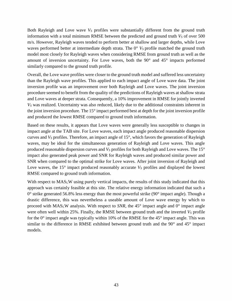
43

Both Rayleigh and Love wave VS profiles were substantially different from the ground truth

information with a total minimum RMSE between the predicted and ground truth VS of over 500

m/s. However, Rayleigh waves tended to perform better at shallow and larger depths, while Love

waves performed better at intermediate depth strata. The 0° VS profile matched the ground truth

model most closely for Rayleigh waves when considering RMSE from ground truth as well as the

amount of inversion uncertainty. For Love waves, both the 90° and 45° impacts performed

similarly compared to the ground truth profile.

Overall, the Love wave profiles were closer to the ground truth model and suffered less uncertainty

than the Rayleigh wave profiles. This applied to each impact angle of Love wave data. The joint

inversion profile was an improvement over both Rayleigh and Love waves. The joint inversion

procedure seemed to benefit from the quality of the predictions of Rayleigh waves at shallow strata

and Love waves at deeper strata. Consequently, a 10% improvement in RMSE for jointly inverted

VS was realized. Uncertainty was also reduced, likely due to the additional constraints inherent in

the joint inversion procedure. The 15° impact performed best at depth for the joint inversion profile

and produced the lowest RMSE compared to ground truth information.

Based on these results, it appears that Love waves were generally less susceptible to changes in

impact angle at the TAB site. For Love waves, each impact angle produced reasonable dispersion

curves and VS profiles. Therefore, an impact angle of 15°, which favors the generation of Rayleigh

waves, may be ideal for the simultaneous generation of Rayleigh and Love waves. This angle

produced reasonable dispersion curves and VS profiles for both Rayleigh and Love waves. The 15°

impact also generated peak power and SNR for Rayleigh waves and produced similar power and

SNR when compared to the optimal strike for Love waves. After joint inversion of Rayleigh and

Love waves, the 15° impact produced reasonably accurate VS profiles and displayed the lowest

RMSE compared to ground truth information.

With respect to MASLW using purely vertical impacts, the results of this study indicated that this

approach was certainly feasible at this site. The relative energy information indicated that such a

0° strike generated 56.8% less energy than the most powerful strike (90° impact angle). Though a

drastic difference, this was nevertheless a useable amount of Love wave energy by which to

proceed with MASLW analysis. With respect to SNR, the 45° impact angle and 0° impact angle

were often well within 25%. Finally, the RMSE between ground truth and the inverted VS profile

for the 0° impact angle was typically within 10% of the RMSE for the 45° impact angle. This was

similar to the difference in RMSE exhibited between ground truth and the 90° and 45° impact

models.

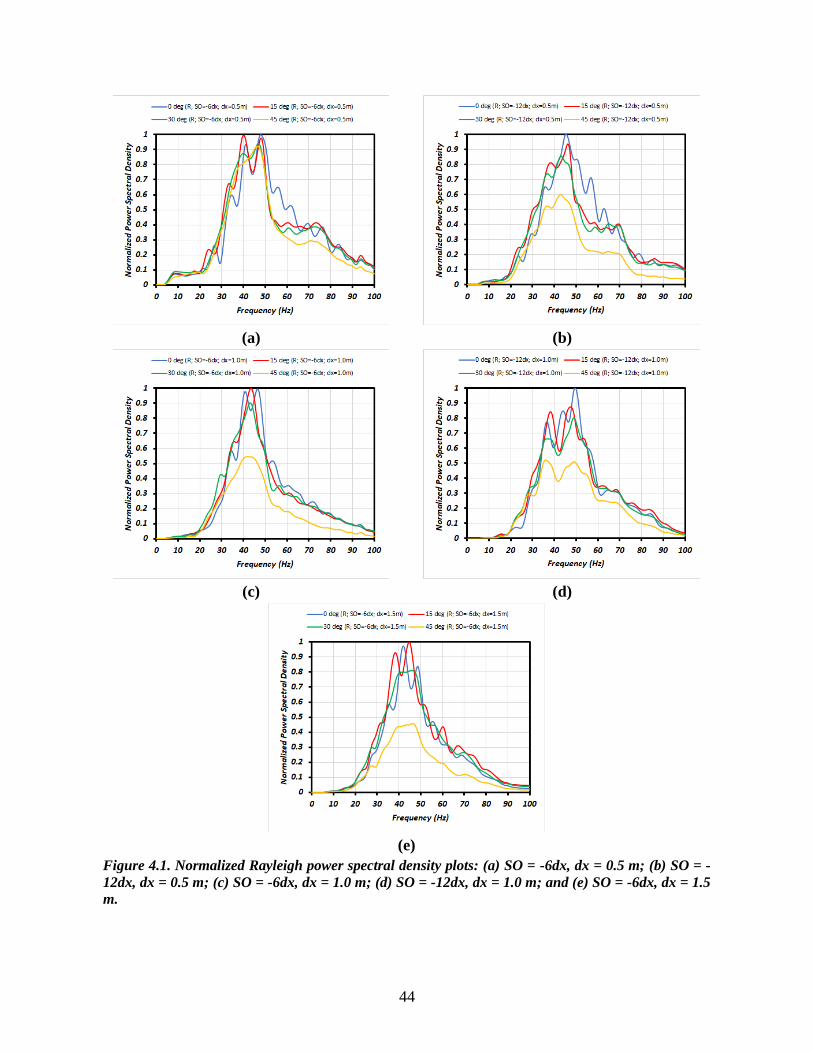
44

(a)

(b)

(c)

(d)

(e)

Figure 4.1. Normalized Rayleigh power spectral density plots: (a) SO = -6dx, dx = 0.5 m; (b) SO = -

12dx, dx = 0.5 m; (c) SO = -6dx, dx = 1.0 m; (d) SO = -12dx, dx = 1.0 m; and (e) SO = -6dx, dx = 1.5

m.

45

(a)

(b)

(c)

(d)

(e)

Figure 4.2. Normalized Love power spectral density plots: (a) SO = -6dx, dx = 0.5 m; (b) SO = -12dx,

dx = 0.5 m; (c) SO = -6dx, dx = 1.0 m; (d) SO = -12dx, dx = 1.0 m; and (e) SO = -6dx, dx = 1.5 m.

46

(a) (b)

(c)

Figure 4.3. Normalized relative energy graphs of Rayleigh waves: (a) SO = -6dx, dx = 1.5 m; (b) SO = -

6dx and -12dx, dx = 1.0 m; (c) SO = -6dx and -12dx, dx = 0.5 m.

47

(a) (b)

(c)

Figure 4.4. Normalized relative energy graphs of Love waves: (a) SO = -6dx, dx = 1.5 m; (b) SO = -6dx

and -12dx, dx = 1.0 m; (c) SO = -6dx and -12dx, dx = 0.5 m.

48

(a) (b)

(c)

Figure 4.5. SNR plots of Rayleigh waves: (a) SO = -6dx, dx = 15 m; (b) SO = -6dx and -12dx, dx = 1.0

m; (c) SO = -6dx and -12dx, dx = 0.5 m.

49

(a) (b)

(c)

Figure 4.6. SNR plots of Love waves: (a) SO = -6dx, dx = 1.5 m; (b) SO = -6dx and -12dx, dx = 1.0 m;

(c) SO = -6dx and -12dx, dx = 0.5 m.

50

(a)

(b)

Figure 4.7. Rayleigh wave dispersion curves compared to the 0° dispersion image: (a) SO = -6dx, dx =

1.5 m; (b) SO = -6dx, dx = 1.0 m.

51

(c)

(d)

Figure 4.7 (cont.). Rayleigh wave dispersion curves compared to the 0° dispersion image: (a) SO = -6dx,

dx = 0.5 m; (b) SO = -12dx, dx = 1.0 m.

52

(e)

Figure 4.7 (cont.). Rayleigh wave dispersion images compared to the 0° dispersion image: (e) SO = -

12dx, dx = 0.5 m.

53

(a)

(b)

Figure 4.8. Love wave dispersion images compared to the 0° dispersion image: (a) SO = -6dx, dx = 1.5

m; (b) SO = -6dx, dx = 1.0 m.

54

(c)

(d)

Figure 4.8 (cont.). Love wave dispersion images compared to the 0° dispersion image: (c) SO = -6dx, dx

= 0.5 m; (d) SO = -12dx, dx = 1.0 m.

55

(e)

Figure 4.8 (cont.). Love wave dispersion images compared to the 90° dispersion image: (e) SO = -12dx,

dx = 0.5.

Figure 4.9. Love wave dispersion curve generated by a 0° impact.

56

(a)

(b)

Figure 4.10. Rayleigh inversion: (a) VS profiles; and (b) difference between inverted VS and ground truth

model VS.

57

(a)

(b)

Figure 4.11. Love wave inversion: (a) VS profiles; and (b) difference between inverted VS and ground

truth model VS.

58

(a)

(b)

Figure 4.12. Joint (Rayleigh and Love) inversion: (a) VS profiles; and (b) difference between inverted VS

and ground truth model VS.

59

Table 4.1. Dominant frequencies in PSD plots for Rayleigh waves.

SO dx 0° 15° 30° 45°

- 6dx

0.5 m

48.0 40.0 46.8 46.4

-12dx 45.4 46.1 43.1 42.9

- 6dx

1.0 m

46.4 43.4 43.1 41.9

-12dx 49.5 47.4 48.9 36.0

- 6dx 1.5 m 42.0 44.6 45.9 46.3

Average 46.26 44.3 45.56 42.7

Difference (%) -4.2% -1.5% -7.7%

Table 4.2. Shape factors (δ) from PSD plots for Rayleigh waves.

SO dx 0° 15° 30° 45°

- 6dx

0.5 m

0.330 0.353 0.355 0.343

-12dx 0.318 0.345 0.340 0.328

- 6dx

1.0 m

0.308 0.322 0.333 0.321

-12dx 0.295 0.316 0.311 0.317

- 6dx 1.5 m 0.294 0.312 0.309 0.308

Average 0.309 0.330 0.329 0.323

Difference (%) 6.5% 6.5% 4.5%

60

Table 4.3. Dominant frequencies in PSD plots for Love waves.

SO dx 90° 45° 30° 15° 0°

- 6dx

0.5 m

37.9 44.7 42.7 38.7 44.8

-12dx 41.3 42 42.7 39 41.8

- 6dx

1.0 m

38.9 37.4 37.9 39.6 36.7

-12dx 49.2 39.2 39.3 38.9 34.1

- 6dx 1.5 m 46.7 48.1 47.6 47.9 41.5

Average 42.8 42.28 42.04 40.82 39.78

Difference (%) -1.2% -1.8% -4.6% -7.1%

Table 4.4. Shape factors (δ) from PSD plots for Love waves.

SO dx 0° 15° 30° 45°

- 6dx

0.5 m

0.385 0.381 0.381 0.368 0.350

-12dx 0.371 0.365 0.362 0.358 0.351

- 6dx

1.0 m

0.365 0.392 0.363 0.354 0.338

-12dx 0.357 0.354 0.337 0.329 0.347

- 6dx 1.5 m 0.352 0.360 0.345 0.327 0.345

Average 0.366 0.370 0.358 0.347 0.346

Difference (%)

1.1% -2.3% -5.2% -5.4%

61

5. CONCLUSIONS

The MASW method is becoming an increasingly popular method of surface wave testing due to

its non-destructive nature and potential to create accurate VS profiles. Studies continue to advance

the methodology but have typically focused on utilizing Rayleigh waves. Several studies have

shown that Love waves can offer distinct advantages over Rayleigh waves. To obtain the best

MASW results, data from both Rayleigh and Love waves should be collected. VS profiles may then

be created by independent and joint inversion, which reduces the uncertainty inherent in the

inversion process. However, the process of collecting Rayleigh and Love wave data separately

significantly increase data acquisition time when using standard MASW procedures because they

are polarized in different directions and require different input sources. Therefore, this study

examined the effectiveness of simultaneous inversion of Rayleigh and Love waves using angled

impacts. Impact angles have been analyzed based on f, SNR, dispersion information, and VS

profiles. This research also examined the effectiveness of vertical impacts for Love wave

generation.

MASW field testing was performed to examine the effectiveness of an angled impact for the

simultaneous generation of Rayleigh and Love waves. Testing was performed at a baseball field

at the Temple Ambler campus site (TAB) approximately 24 km north of Center City Philadelphia.

A set of 24 geophone receivers was used to collect surface wave data from impacts were performed

at angles of 0°, 15°, 30°, 45°, and 90°. The 90° impact was not used to generate Rayleigh waves

due to logistical issues. An AWD was used to produce impacts on all sources but the 90° source,

where a 20 lb sledgehammer was utilized.

Following data collection, data was processed using a combination of custom MATLAB scripts,

the Geometrics SeisImager/SW® commercial software package, and the open-source Geopsy

software package. The phase-shift method (Park et al., 1998) was used to generate dispersion

images and both independent and joint inversions were performed to produce VS profiles. These

VS profiles were subsequently compared to ground truth information obtained from previous

seismic refraction and downhole testing.

5.1. Goals of Project

The goals of this research effort were to provide recommendations regarding the optimal impact

angle for the simultaneous generation of Rayleigh and Love wave and to examine the effectiveness

of a vertical strike for Love wave generation. The following conclusions can be drawn after an

analysis of f, power, SNR, dispersion curves, and VS profiles:

• A 15° impact produced the highest normalized relative energy for Rayleigh waves. A 30°

impact produced the highest normalized relative energy for Love waves. However, a 15°

impact generated just 11.8% less energy for Love waves. A 15° impact also produced the

highest SNR and fdom for Rayleigh waves. The 15° impact performed within 5% of the

optimal angle (i.e. 30°) for Love wave generation. Therefore, at the TAB site, a 15° impact

62

is recommended for maximum energy during simultaneous generation of Rayleigh and

Love waves.

• A vertical strike (i.e., 0°) generated 56.8% less Love wave energy than the most powerful

strike at 30 degrees.

• Dominant frequencies and SNR were only moderately affected by changes in impact angle

for both Rayleigh and Love waves. Average fdom and average SNR changed by no more

than 10% between different impact angles.

• The Love wave dispersion curve generated by vertical strikes matched reasonably well

with the dispersion curve generated by an ideal impact angle (i.e., 90°). This result indicates

that vertical strikes may be effective for Love wave generation.

• The Love wave overtone images were significantly clearer than the Rayleigh wave images,

especially in terms of fundamental-mode identification. Love wave dispersion curves also

matched reasonably well between different data sets, even as the impact angle approached

vertical.

• Neither Rayleigh nor Love waves provided VS profiles that matched well with the ground

truth model. Rayleigh waves performed well at the near surface, however, uncertainty and

misfit increased with depth. Love waves performed better overall, particularly in the

intermediate range of depths. Love wave VS profiles were also significantly less impacted

by changes in impact angle.

• Overall, Love waves were less affected by changes in impact angle. Because Rayleigh

waves are more affected by source angle at the TAB site, the optimal impact angle should

be governed by Rayleigh waves.

This research effort showed that, at the TAB site examined in this study, Love waves were

significantly less affected by changes in impact angle than were Rayleigh waves. Even as the

impact angle moved towards vertical, Love wave generation still occurred and reasonable

dispersion images were obtained. This conclusion may prove valid across a wide range of site

conditions due to the inherent properties of Love wave generation. Near-vertical impacts seem to

produce sizable horizontal wave components, especially as the wave propagates farther from the

impact source. This effect may be caused by the restorative force of gravity that pulls near-vertical

waves towards horizontal. Love wave generation could benefit significantly from this effect and,

as a result, the optimal angle for simultaneous generation may be inclined more towards vertical.

63

6. REFERENCES

Abbiss, C.P. (1981). “Shear wave measurements of the elasticity of the ground.” Geotechnique,

31(1), 91-109.

Cox, B. R., and Teague, D. P. (2016). “Layering ratios: a systematic approach to the inversion of

surface wave data in the absence of a priori information.” Geophysical Journal

International, 207(1), 422-438.

Dal Moro, G., and Ferigo, F. (2011). “Joint analysis of Rayleigh-and Love-wave dispersion:

Issues, criteria and improvements.” Journal of Applied Geophysics, 75(3), 573-589.

Eslick, R., Tsoflias, G., and Steeples, D. (2007). “Field investigations of Love waves in near-

surface seismology.” Geophysics, 73(3), G1–G6.

Foti, S., Hollender, F., Garofalo, F. et al. (2018). “Guidelines for the good practice of surface wave

analysis: a product of the InterPACIFIC project.” Bull. Earthquake Eng., 16, 2367–2420.

Gaiser, J. (2016). 3C Seismic and VSP: Converted waves and vector wavefield applications.

Society of Exploration Geophysicists, Tulsa, OK, 636 pp.

Haines, S. S. (2007). A hammer-impact, aluminum, shear-wave seismic source. Open-File Report

2007–1406, U.S. Department of Interior, U.S. Geological Survey, Reston, VA.

Hardage, B. A., DeAngelo, M. V., Murray, P. E., and Sava, D. (2011). Multicomponent seismic

technology. Society of Exploration Geophysicists, Tulsa, OK, 335 pp.

Häusler, M., Schmelzbach, C., and Sollberger, D. (2018). “The Galperin source: A novel efficient

multicomponent seismic source.” Geophysics, 83(6), P19-P27.

Heisey, J.S., Stokoe II, K.H., and Meyer, A.H. (1982). “Moduli of pavement systems from Spectral

Analysis of Surface Waves.” Transp. Res. Rec., 852, 22-31.

Jones, R. (1955). “A Vibration Method for Measuring the Thickness of Concrete Road Slabs In

Situ.” Magazine of Concrete Research, 7(20), 97-102.

Jones, R. (1958). “In situ measurement of the dynamic properties of soil by vibration methods.”

Geotechnique, 8(1), 1-21.

Julia, J., Ammon, C.J., Herrman, R.B., and Correig, A.M. (2000). “Joint inversion of receiver

function and surface wave dispersion observations.” Geophysical Journal International, 143, 99–

112.

Lay, T., and Wallace. T. C. (1995). Model Global Seismology. Oxford, United Kingdom,

Academic Press.

J.L. Mari. (1984). “Estimation of static corrections for shear-wave profiling using the dispersion

properties of Love waves.” Geophysics, 49(8), 1169-1179.

Kramer, S.L. (1996). Geotechnical Earthquake Engineering. Pearson, New Jersey, 653 pp.

64

Love, A.E. (1911). Some problems of geodynamics. Cambridge University Press.

Mahvelati, S., (2019). Advancements in Surface Wave Testing: Numerical, Laboratory, and Field

Investigations Regarding the Effects of Input Source and Survey Parameters on Rayleigh and Love

Waves. Ph.D. Dissertation, Temple University.

Mahvelati, S. and Coe., J. T. (2017). “Multichannel Analysis of Surface Waves (MASW) Using

Both Rayleigh and Love Waves to Characterize Site Conditions.” Proceedings Geotechnical

Frontiers, 647-656.

Matthews, M.C., Hope, V.S. and Clayton, C.R.I. (1996). “The use of surface waves in the

determination of ground stiffness profiles.” Proc. Institution of Civil Engineers Geotech.

Engineering., 119, 84-95.

Miller, R.D., Pullan, S.E., Waldner, J.S., and Haeni, F.P. (1986). “Field comparison of shallow

seismic sources.” Geophysics, 51(11), 2067-2092.

McMechan, G. A., and Yedlin, M. J. (1981). “Analysis of dispersive waves by wave field

transformation.” Geophysics, 46(6), 869-874.

Ólafsdóttir, Á. E. (2014). Multichannel Analysis of Surface Waves: Methods for dispersion

analysis of surface wave data. University of Iceland: School of Engineering and Natural Sciences,

76 pp.

Olafsdottir, E. A., Bessason, B., and Erlingsson, S. (2018). “Combination of dispersion curves

from MASW measurements.” Soil Dynamics and Earthquake Engineering, 113, 473-487.

Park, C.B., Miller, R.D., and Xia, J. (1998). “Imaging dispersion curves of surface waves on multi-

channel record.” 68th Ann. Internat. Mtg. Soc. Expl. Geophys., 1377-1380.

Park, C.B., Miller, R.D., and Miura H. (2002). “Optimum field parameters of an MASW survey.”

Japanese Society of Exploration Geophysics Extended Abstracts, 1-6.

Park, C.B., Miller, R.D., Xia, J., and Ivanov., J. (2007). “Multichannel analysis of surface waves

(MASW) – active and passive methods.” The Leading Edge, 26(1), 60-64.

Pei, D. (2007). Modeling and inversion of dispersion curves of surface waves in shallow site

investigations. Ph.D Dissertation, University of Nevada, Reno.

Rossi, G., and Vesnaver, A. (1997). “3-D imaging by adaptive joint inversion of reflected and

refracted arrivals.” SEG Technical Program Expanded Abstracts, 1873-1876.

Safani, J., O’Neill, A., Matsuoka, T., and Sanada, Y. (2005). “Applications of Love wave

dispersion for improved shear-wave velocity imaging.” Journal of Environmental Engineering

Geophysics, 10(2), 135–150.

Schmelzbach, C., Sollberger, D., Greenhalgh, S. A., Horstmeyer, H., Maurer, H., and Robertsson,

J. O. (2016). “9C seismic data acquisition for near-surface applications: Recording, waveform

reciprocity and 4C rotation.” 78th EAGE Conference and Exhibition, 1-5.

65

Socco, L.V., Foti, S., and Boiero, D. (2010). “Surface-wave analysis for building near-surface

velocity models – Established approaches and new perspectives.” Geophysics, 75(5), 75A83-

75A102.

Song, Y. Y., Castagna, J. P., Black, R. A., and Knapp, R. W. (1989). “Sensitivity of Near-Surface

Shear-Wave Velocity Determination from Rayleigh and Love Waves.” Proc. SEG 59th Ann. Mtg.,

Dallas, TX, 509-512.

Tokimatsu, K., Kuwayama, S., Tamura, S. and Miyadera, Y. (1991). “VS determination from

steady state Rayleigh wave method.” Soils and Foundations, 31(2), 153-163.

Van der Pol, C. (1951). “Dynamic Testing of Road Constructions.” Journal of Applied Chemistry,

1, 281-290.

Vanmarcke, E.H. (1976). “Structural response to earthquakes.” Seismic Risk and Engineering

Decisions, C. Lomnitz and E. Rosenblueth (Eds.), 287-338.

Vozoff, K., and Jupp, D.L.B. (1975). “Joint Inversion of Geophysical Data.” Geophys. J. Int., 42,

977–991.

Wathelet, M. (2005). Array Recordings of Ambient Vibrations: Surface-wave Inversion. PhD

Dissertation, Liège University, 177 pp.

Wathelet, M. (2008). “An improved neighborhood algorithm: parameter conditions and dynamic

scaling.” Geophysical Research Letters, 35, L09301, doi: 10.1029/2008GL033256.

Wathelet, M., Chatelain, J.-L., Cornou, C., Di Giulio, G., Guillier, B., Ohrnberger, M. and

Savvaidis, A. (2020). “Geopsy: A User-Friendly Open-Source Tool Set for Ambient Vibration

Processing.” Seismological Research Letters, 91(3), 1878–1889.

Xia, J., Miller, R. D., and Park, C. B. (2000). “Advantages of calculating shear-wave velocity from

surface waves with higher modes.” SEG Technical Program Expanded Abstracts, 1295-1298.

Xia, J., Xu, Y., Luo, Y., Miller, R. D., Cakir, R., and Zeng, C. (2012). “Advantages of using

multichannel analysis of Love waves (MALW) to estimate near-surface shear-wave

velocity.” Surveys in Geophysics, 33(5), 841-860.

Xia, J., Miller, R. D., and Park, C. B. (1999). “Estimation of near-surface shear-wave velocity by

inversion of Rayleigh waves.” Geophysics, 64(3), 691–700.

Yin, X., Xia, J., Shen, C., and Xu, H. (2014). “Comparative analysis on penetrating depth of high-

frequency Rayleigh and Love waves.” J. Appl. Geophys., 111, 86-94.

Yong, A., Martin, A., Stokoe, K., and Diehl, J. (2013). ARRA-Funded VS30 Measurements Using

Multi-Technique Approach at Strong-Motion Stations in California and Central-Eastern United

States. U.S. Geological Survey Open-File Report 2013–1102, 60 p. and data files,

http://pubs.usgs.gov/of/2013/1102/.

http://pubs.usgs.gov/of/2013/1102/

66

Yoon, S., and Rix, G. J. (2009). “Near-field effects on array-based surface wave methods with

active sources.” Journal of Geotechnical and Geoenvironmental Engineering, 135(3), 399-406.

simultaneous rayleigh and love wave acquisition for joint ...

Documents