Simultaneous Equation Econometrics: The Missing Example Dennis Epple Carnegie Mellon University and NBER and Bennett T. McCallum Carnegie Mellon University and NBER February 12, 2004 Revised January 7, 2005 ABSTRACT: For introductory presentation of issues involving identification and estimation of simultaneous equation systems, a natural vehicle is a model consisting of supply and demand relationships to explain price and quantity variables for a single good. One would accordingly expect to find in introductory econometrics textbooks a supply-demand example featuring actual data in which structural estimation methods yield more satisfactory results than ordinary least squares. In a search of 26 existing textbooks, however, we have found no such example—indeed, no example with actual data in which all parameter estimates are of the proper sign and statistically significant. This absence is documented in the present paper. Its main contribution, however, is the development of a simple but satisfying example, for broiler chickens, based on U.S. annual data over 1960-1999. Some discussion of the historically notable beef example of Tintner (1952) is included. The authors are indebted to Edward Nelson and Holger Sieg for helpful suggestions.

Welcome message from author
This document is posted to help you gain knowledge. Please leave a comment to let me know what you think about it! Share it to your friends and learn new things together.
Transcript
Simultaneous Equation Econometrics: The Missing Example
Dennis Epple
Carnegie Mellon University and NBER
and
Bennett T. McCallum
Carnegie Mellon University and NBER
February 12, 2004
Revised January 7, 2005
ABSTRACT: For introductory presentation of issues involving identification and estimation of simultaneous equation systems, a natural vehicle is a model consisting of supply and demand relationships to explain price and quantity variables for a single good. One would accordingly expect to find in introductory econometrics textbooks a supply-demand example featuring actual data in which structural estimation methods yield more satisfactory results than ordinary least squares. In a search of 26 existing textbooks, however, we have found no such example—indeed, no example with actual data in which all parameter estimates are of the proper sign and statistically significant. This absence is documented in the present paper. Its main contribution, however, is the development of a simple but satisfying example, for broiler chickens, based on U.S. annual data over 1960-1999. Some discussion of the historically notable beef example of Tintner (1952) is included.
The authors are indebted to Edward Nelson and Holger Sieg for helpful suggestions.
1
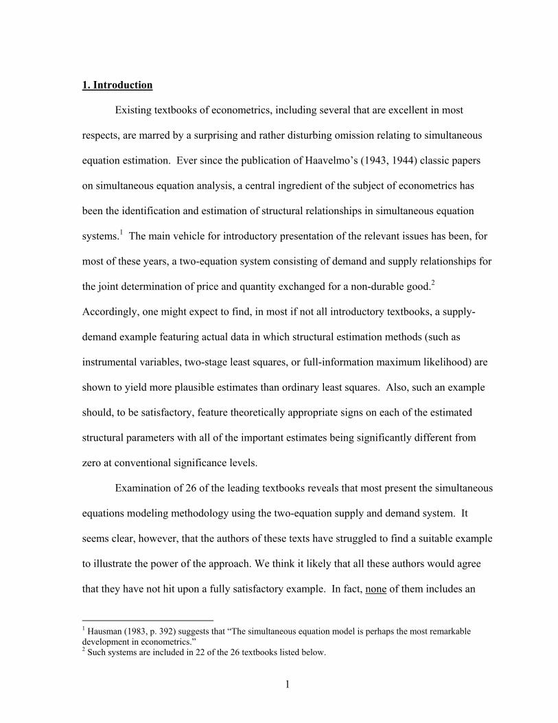
1. Introduction
Existing textbooks of econometrics, including several that are excellent in most
respects, are marred by a surprising and rather disturbing omission relating to simultaneous
equation estimation. Ever since the publication of Haavelmo’s (1943, 1944) classic papers
on simultaneous equation analysis, a central ingredient of the subject of econometrics has
been the identification and estimation of structural relationships in simultaneous equation
systems.1 The main vehicle for introductory presentation of the relevant issues has been, for
most of these years, a two-equation system consisting of demand and supply relationships for
the joint determination of price and quantity exchanged for a non-durable good.2
Accordingly, one might expect to find, in most if not all introductory textbooks, a supply-
demand example featuring actual data in which structural estimation methods (such as
instrumental variables, two-stage least squares, or full-information maximum likelihood) are
shown to yield more plausible estimates than ordinary least squares. Also, such an example
should, to be satisfactory, feature theoretically appropriate signs on each of the estimated
structural parameters with all of the important estimates being significantly different from
zero at conventional significance levels.
Examination of 26 of the leading textbooks reveals that most present the simultaneous
equations modeling methodology using the two-equation supply and demand system. It
seems clear, however, that the authors of these texts have struggled to find a suitable example
to illustrate the power of the approach. We think it likely that all these authors would agree
that they have not hit upon a fully satisfactory example. In fact, none of them includes an
1 Hausman (1983, p. 392) suggests that “The simultaneous equation model is perhaps the most remarkable development in econometrics.” 2 Such systems are included in 22 of the 26 textbooks listed below.
2
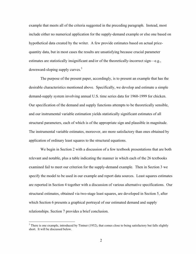
example that meets all of the criteria suggested in the preceding paragraph. Instead, most
include either no numerical application for the supply-demand example or else one based on
hypothetical data created by the writer. A few provide estimates based on actual price-
quantity data, but in most cases the results are unsatisfying because crucial parameter
estimates are statistically insignificant and/or of the theoretically-incorrect sign—e.g.,
downward-sloping supply curves.3
The purpose of the present paper, accordingly, is to present an example that has the
desirable characteristics mentioned above. Specifically, we develop and estimate a simple
demand-supply system involving annual U.S. time series data for 1960-1999 for chicken.
Our specification of the demand and supply functions attempts to be theoretically sensible,
and our instrumental variable estimation yields statistically significant estimates of all
structural parameters, each of which is of the appropriate sign and plausible in magnitude.
The instrumental variable estimates, moreover, are more satisfactory than ones obtained by
application of ordinary least squares to the structural equations.
We begin in Section 2 with a discussion of a few textbook presentations that are both
relevant and notable, plus a table indicating the manner in which each of the 26 textbooks
examined fail to meet our criterion for the supply-demand example. Then in Section 3 we
specify the model to be used in our example and report data sources. Least squares estimates
are reported in Section 4 together with a discussion of various alternative specifications. Our
structural estimates, obtained via two-stage least squares, are developed in Section 5, after
which Section 6 presents a graphical portrayal of our estimated demand and supply
relationships. Section 7 provides a brief conclusion.
3 There is one example, introduced by Tintner (1952), that comes close to being satisfactory but falls slightly short. It will be discussed below.
3
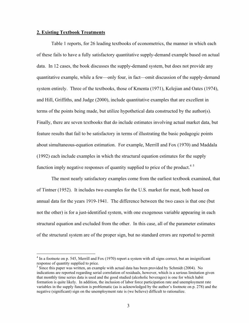
2. Existing Textbook Treatments
Table 1 reports, for 26 leading textbooks of econometrics, the manner in which each
of these fails to have a fully satisfactory quantitative supply-demand example based on actual
data. In 12 cases, the book discusses the supply-demand system, but does not provide any
quantitative example, while a few—only four, in fact—omit discussion of the supply-demand
system entirely. Three of the textbooks, those of Kmenta (1971), Kelejian and Oates (1974),
and Hill, Griffiths, and Judge (2000), include quantitative examples that are excellent in
terms of the points being made, but utilize hypothetical data constructed by the author(s).
Finally, there are seven textbooks that do include estimates involving actual market data, but
feature results that fail to be satisfactory in terms of illustrating the basic pedagogic points
about simultaneous-equation estimation. For example, Merrill and Fox (1970) and Maddala
(1992) each include examples in which the structural equation estimates for the supply
function imply negative responses of quantity supplied to price of the product.4 5
The most nearly satisfactory examples come from the earliest textbook examined, that
of Tintner (1952). It includes two examples for the U.S. market for meat, both based on
annual data for the years 1919-1941. The difference between the two cases is that one (but
not the other) is for a just-identified system, with one exogenous variable appearing in each
structural equation and excluded from the other. In this case, all of the parameter estimates
of the structural system are of the proper sign, but no standard errors are reported to permit
4 In a footnote on p. 545, Merrill and Fox (1970) report a system with all signs correct, but an insignificant response of quantity supplied to price. 5 Since this paper was written, an example with actual data has been provided by Schmidt (2004). No indications are reported regarding serial correlation of residuals, however, which is a serious limitation given that monthly time series data is used and the good studied (alcoholic beverages) is one for which habit formation is quite likely. In addition, the inclusion of labor force participation rate and unemployment rate variables in the supply function is problematic (as is acknowledged by the author’s footnote on p. 278) and the negative (significant) sign on the unemployment rate is (we believe) difficult to rationalize.

4
Table 1: Supply-Demand Examples in Existing Textbooks
Author(s)
Date
No S&DExample
No Numer.Example
Hypoth.Data
Incorrect Sign
Non- Significant
Tintner 1952 1 2 Klein 1953 *
Valavanis 1959 * Klein 1962 *
Johnston 1963 * Goldberger 1964 3 3
Christ 1966 * Malinvaud 1966 4
Merrill and Fox 1970 * * Theil 1971 * Frank 1971 *
Kmenta 1971 * 5 Beals 1972 7
Murphy 1973 Kelejian & Oates 1974 *
Pindyck & Rubinfeld 1976 * Maddala 1977 *
Wonnacott&Wonnacott 1979 * Kennedy 1979 *
Wallace & Silver 1988 * Maddala 1992 * Gujarati 1995 6
Johnston & DiNardo 1997 * Hill, Griffiths, & Judge 2001 *
Wooldridge 2003 * Ashenfelter, et. al. 2003 *
Notes: 1. Overidentified example on pp. 177-184; see Goldberger, p. 328 . 2. Just identified example on pp. 168-172; no standard errors reported. 3. Tintner’s overidentified example. 4. A demand function is estimated, but no supply function. 5. Tintner’s just-identified example. 6. Incomplete example; one equation only. 7. Data (whether artificial or actual is unclear) provided only in problem.
5
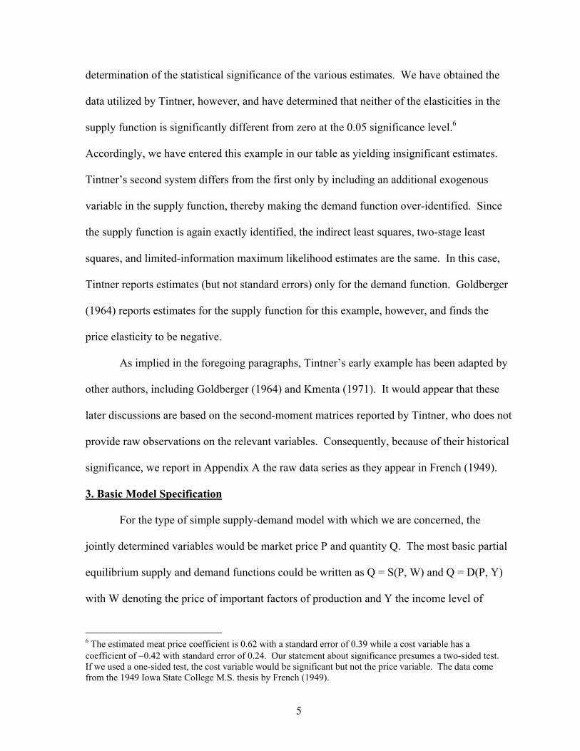
determination of the statistical significance of the various estimates. We have obtained the
data utilized by Tintner, however, and have determined that neither of the elasticities in the
supply function is significantly different from zero at the 0.05 significance level.6
Accordingly, we have entered this example in our table as yielding insignificant estimates.
Tintner’s second system differs from the first only by including an additional exogenous
variable in the supply function, thereby making the demand function over-identified. Since
the supply function is again exactly identified, the indirect least squares, two-stage least
squares, and limited-information maximum likelihood estimates are the same. In this case,
Tintner reports estimates (but not standard errors) only for the demand function. Goldberger
(1964) reports estimates for the supply function for this example, however, and finds the
price elasticity to be negative.
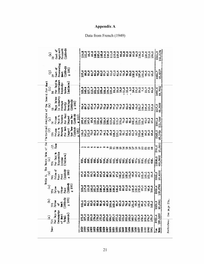
As implied in the foregoing paragraphs, Tintner’s early example has been adapted by
other authors, including Goldberger (1964) and Kmenta (1971). It would appear that these
later discussions are based on the second-moment matrices reported by Tintner, who does not
provide raw observations on the relevant variables. Consequently, because of their historical
significance, we report in Appendix A the raw data series as they appear in French (1949).
3. Basic Model Specification
For the type of simple supply-demand model with which we are concerned, the
jointly determined variables would be market price P and quantity Q. The most basic partial
equilibrium supply and demand functions could be written as Q = S(P, W) and Q = D(P, Y)
with W denoting the price of important factors of production and Y the income level of
6 The estimated meat price coefficient is 0.62 with a standard error of 0.39 while a cost variable has a coefficient of −0.42 with standard error of 0.24. Our statement about significance presumes a two-sided test. If we used a one-sided test, the cost variable would be significant but not the price variable. The data come from the 1949 Iowa State College M.S. thesis by French (1949).
6
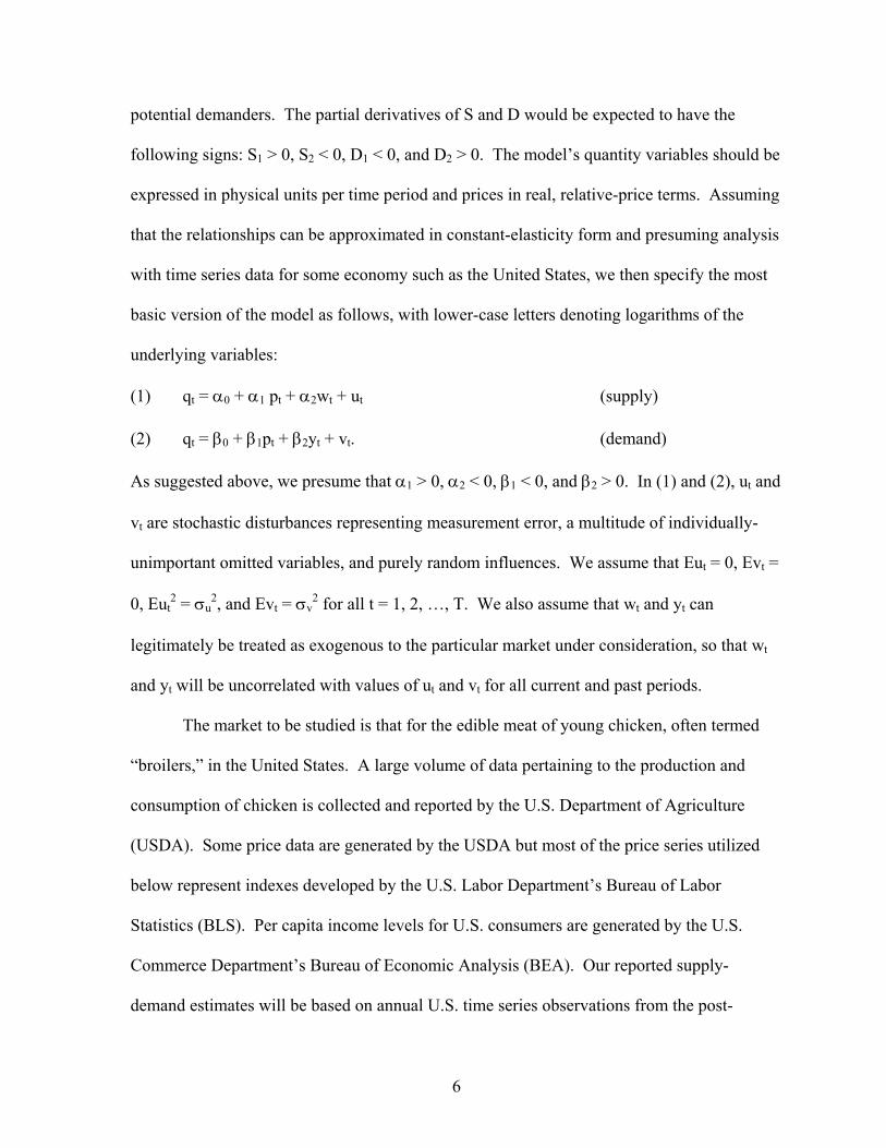
potential demanders. The partial derivatives of S and D would be expected to have the
following signs: S1 > 0, S2 < 0, D1 < 0, and D2 > 0. The model’s quantity variables should be
expressed in physical units per time period and prices in real, relative-price terms. Assuming
that the relationships can be approximated in constant-elasticity form and presuming analysis
with time series data for some economy such as the United States, we then specify the most
basic version of the model as follows, with lower-case letters denoting logarithms of the
underlying variables:
(1) qt = α0 + α1 pt + α2wt + ut (supply)
(2) qt = β0 + β1pt + β2yt + vt. (demand)
As suggested above, we presume that α1 > 0, α2 < 0, β1 < 0, and β2 > 0. In (1) and (2), ut and
vt are stochastic disturbances representing measurement error, a multitude of individually-
unimportant omitted variables, and purely random influences. We assume that Eut = 0, Evt =
0, Eut2 = σu
2, and Evt = σv2 for all t = 1, 2, …, T. We also assume that wt and yt can
legitimately be treated as exogenous to the particular market under consideration, so that wt
and yt will be uncorrelated with values of ut and vt for all current and past periods.
The market to be studied is that for the edible meat of young chicken, often termed
“broilers,” in the United States. A large volume of data pertaining to the production and
consumption of chicken is collected and reported by the U.S. Department of Agriculture
(USDA). Some price data are generated by the USDA but most of the price series utilized
below represent indexes developed by the U.S. Labor Department’s Bureau of Labor
Statistics (BLS). Per capita income levels for U.S. consumers are generated by the U.S.
Commerce Department’s Bureau of Economic Analysis (BEA). Our reported supply-
demand estimates will be based on annual U.S. time series observations from the post-
7
World-War-II era, with the exact dates (reported below) determined by data availability.
Our aim is to obtain satisfactory estimates of basic structural equations such as (1)
and (2), keeping the specifications as simple as possible. Some possible complexities must,
however, be recognized. One is due to the rapid improvements in technology for the
production of broilers that have taken place over the postwar era, thereby shifting the supply
function. Also, there have been major changes in the price of chicken relative to those for
other types of meat, so the price of some substitute goods might be expected to appear in the
demand function. In addition, the improvement of transportation facilities has been so rapid
that in recent years it has become the case that a significant fraction of U.S. broiler
production is exported abroad, primarily to Russia and Hong Kong.
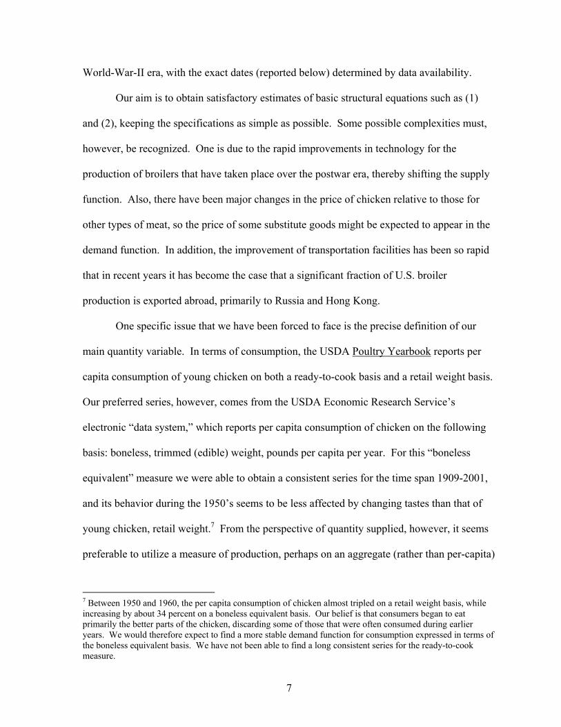
One specific issue that we have been forced to face is the precise definition of our
main quantity variable. In terms of consumption, the USDA Poultry Yearbook reports per
capita consumption of young chicken on both a ready-to-cook basis and a retail weight basis.
Our preferred series, however, comes from the USDA Economic Research Service’s
electronic “data system,” which reports per capita consumption of chicken on the following
basis: boneless, trimmed (edible) weight, pounds per capita per year. For this “boneless
equivalent” measure we were able to obtain a consistent series for the time span 1909-2001,
and its behavior during the 1950’s seems to be less affected by changing tastes than that of
young chicken, retail weight.7 From the perspective of quantity supplied, however, it seems
preferable to utilize a measure of production, perhaps on an aggregate (rather than per-capita)
7 Between 1950 and 1960, the per capita consumption of chicken almost tripled on a retail weight basis, while increasing by about 34 percent on a boneless equivalent basis. Our belief is that consumers began to eat primarily the better parts of the chicken, discarding some of those that were often consumed during earlier years. We would therefore expect to find a more stable demand function for consumption expressed in terms of the boneless equivalent basis. We have not been able to find a long consistent series for the ready-to-cook measure.
8
basis. The way in which we face this difficulty will be detailed in Section 5 below, and the
itemization of the precise series used for the various variables will be provided in Appendix
B together with the data series themselves.
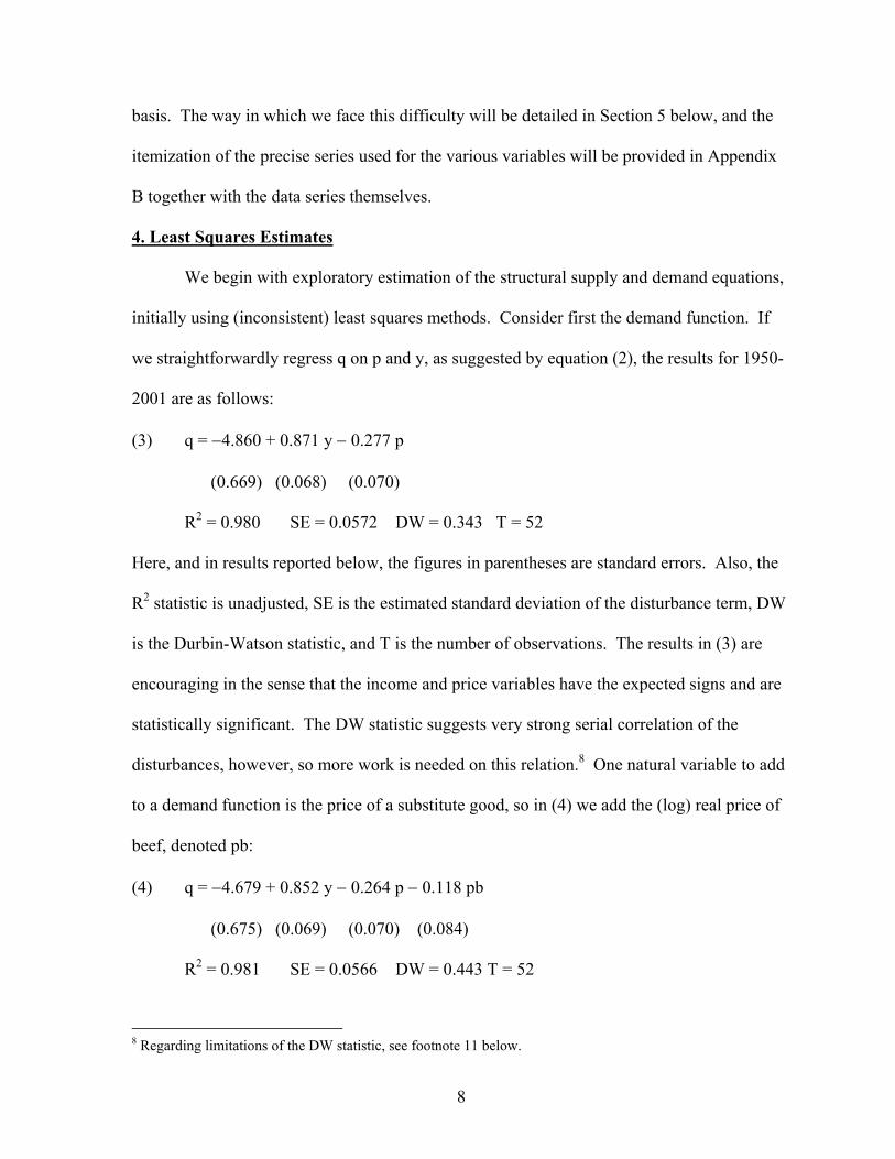
4. Least Squares Estimates
We begin with exploratory estimation of the structural supply and demand equations,
initially using (inconsistent) least squares methods. Consider first the demand function. If
we straightforwardly regress q on p and y, as suggested by equation (2), the results for 1950-
2001 are as follows:
(3) q = −4.860 + 0.871 y − 0.277 p
(0.669) (0.068) (0.070)
R2 = 0.980 SE = 0.0572 DW = 0.343 T = 52
Here, and in results reported below, the figures in parentheses are standard errors. Also, the
R2 statistic is unadjusted, SE is the estimated standard deviation of the disturbance term, DW
is the Durbin-Watson statistic, and T is the number of observations. The results in (3) are
encouraging in the sense that the income and price variables have the expected signs and are
statistically significant. The DW statistic suggests very strong serial correlation of the
disturbances, however, so more work is needed on this relation.8 One natural variable to add
to a demand function is the price of a substitute good, so in (4) we add the (log) real price of
beef, denoted pb:
(4) q = −4.679 + 0.852 y − 0.264 p − 0.118 pb
(0.675) (0.069) (0.070) (0.084)
R2 = 0.981 SE = 0.0566 DW = 0.443 T = 52
8 Regarding limitations of the DW statistic, see footnote 11 below.

9
Here pb enters with the wrong sign (for a substitute) and the DW is still unacceptably low,
indicating very strong autocorrelation. Thus we specify the disturbance term as following a
first-order autoregressive [AR(1)] process and obtain the following:9
(5) q = 5.939 + 0.272 y − 0.307 p + 0.247 pb + 0.997 u(-1)
(0.188) (0.272) (0.070) (0.084) (0.019)
R2 = 0.995 SE = 0.0288 DW = 2.396 T = 51
Now the price of beef enters significantly and with the correct sign, and the residual
autocorrelation is greatly reduced. The value of the estimated AR(1) parameter for the
disturbance is so close to 1.0, however, that we are led to impose the value 1.0 and estimate
the equation in first-difference form. No constant term is included, since it would represent a
time trend in the log-levels regression. Our results are:
(6) ∆q = 0.711 ∆y − 0.374 ∆p + 0.251 ∆pb
(0.150) (0.058) (0.068)
R2 = 0.331 SE = 0.0294 DW = 2.38 T = 51
Here the R2 statistic is much smaller, but pertains to a different dependent variable.10 The SE
statistic indicates more informatively that the equation’s explanatory power is almost as high
as for (5). All variables have the theoretically appropriate signs and there is no strong
indication of autocorrelated disturbances. Consequently, we adopt (6) as a promising
demand specification to carry into our simultaneous-equation estimation attempts to be made
below.
Turning now to the chicken supply function, we begin with a counterpart to (1)
above, with pcor representing the real price of corn, an important input price since corn is the
9 Use of the AR(1) specification for vt leads to loss of the observation for 1950. 10 The implied R2 for q is 0.994. Analogous values for all demand functions below exceed 0.992.
10
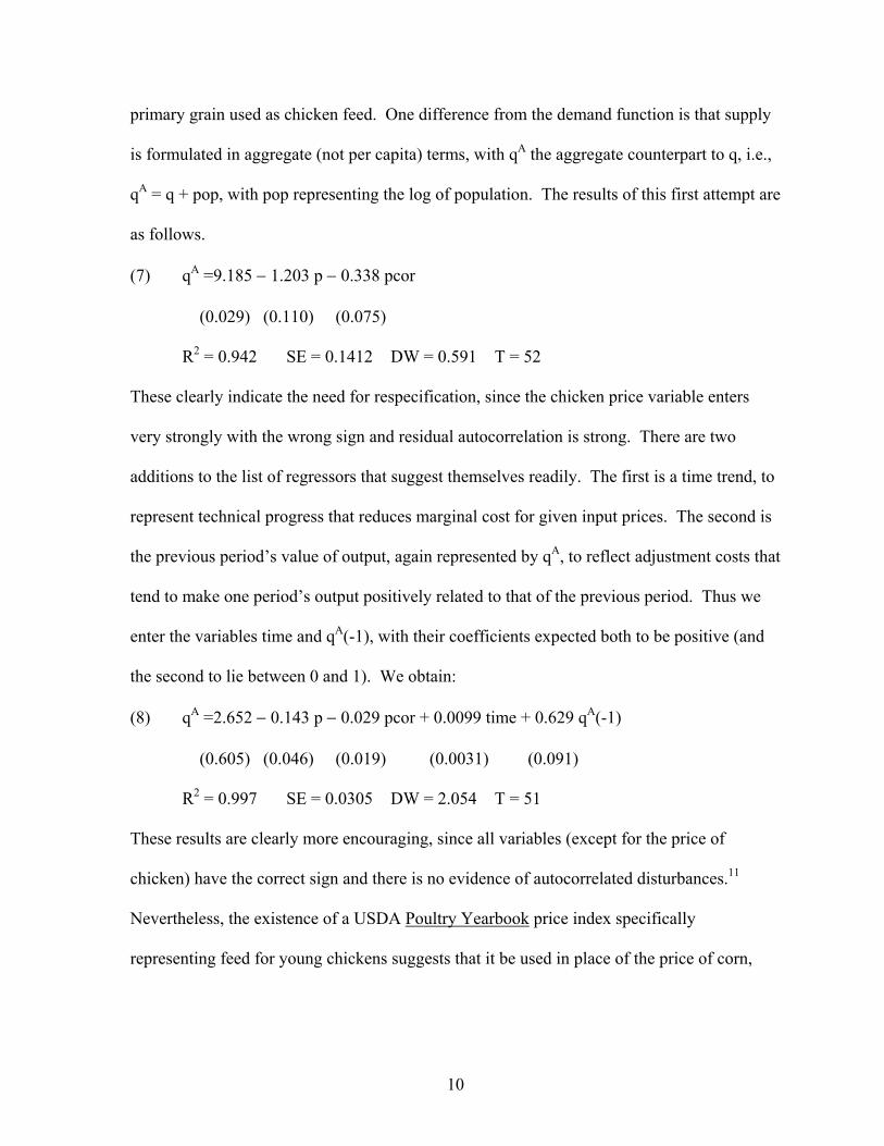
primary grain used as chicken feed. One difference from the demand function is that supply
is formulated in aggregate (not per capita) terms, with qA the aggregate counterpart to q, i.e.,
qA = q + pop, with pop representing the log of population. The results of this first attempt are
as follows.
(7) qA =9.185 − 1.203 p − 0.338 pcor
(0.029) (0.110) (0.075)
R2 = 0.942 SE = 0.1412 DW = 0.591 T = 52
These clearly indicate the need for respecification, since the chicken price variable enters
very strongly with the wrong sign and residual autocorrelation is strong. There are two
additions to the list of regressors that suggest themselves readily. The first is a time trend, to
represent technical progress that reduces marginal cost for given input prices. The second is
the previous period’s value of output, again represented by qA, to reflect adjustment costs that
tend to make one period’s output positively related to that of the previous period. Thus we
enter the variables time and qA(-1), with their coefficients expected both to be positive (and
the second to lie between 0 and 1). We obtain:
(8) qA =2.652 − 0.143 p − 0.029 pcor + 0.0099 time + 0.629 qA(-1)
(0.605) (0.046) (0.019) (0.0031) (0.091)
R2 = 0.997 SE = 0.0305 DW = 2.054 T = 51
These results are clearly more encouraging, since all variables (except for the price of
chicken) have the correct sign and there is no evidence of autocorrelated disturbances.11
Nevertheless, the existence of a USDA Poultry Yearbook price index specifically
representing feed for young chickens suggests that it be used in place of the price of corn,
11
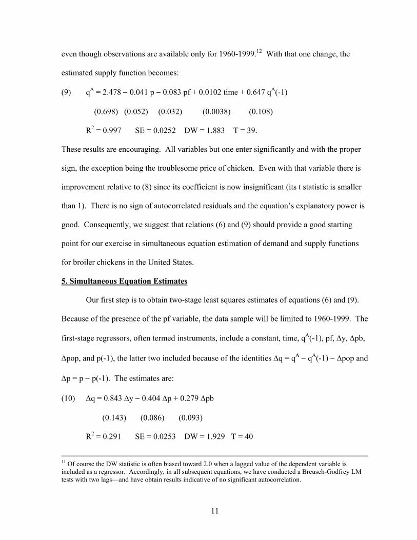
even though observations are available only for 1960-1999.12 With that one change, the
estimated supply function becomes:
(9) qA = 2.478 − 0.041 p − 0.083 pf + 0.0102 time + 0.647 qA(-1)
(0.698) (0.052) (0.032) (0.0038) (0.108)
R2 = 0.997 SE = 0.0252 DW = 1.883 T = 39.
These results are encouraging. All variables but one enter significantly and with the proper
sign, the exception being the troublesome price of chicken. Even with that variable there is
improvement relative to (8) since its coefficient is now insignificant (its t statistic is smaller
than 1). There is no sign of autocorrelated residuals and the equation’s explanatory power is
good. Consequently, we suggest that relations (6) and (9) should provide a good starting
point for our exercise in simultaneous equation estimation of demand and supply functions
for broiler chickens in the United States.
5. Simultaneous Equation Estimates
Our first step is to obtain two-stage least squares estimates of equations (6) and (9).
Because of the presence of the pf variable, the data sample will be limited to 1960-1999. The
first-stage regressors, often termed instruments, include a constant, time, qA(-1), pf, ∆y, ∆pb,
∆pop, and p(-1), the latter two included because of the identities ∆q = qA − qA(-1) − ∆pop and
∆p = p − p(-1). The estimates are:
(10) ∆q = 0.843 ∆y − 0.404 ∆p + 0.279 ∆pb
(0.143) (0.086) (0.093)
R2 = 0.291 SE = 0.0253 DW = 1.929 T = 40
11 Of course the DW statistic is often biased toward 2.0 when a lagged value of the dependent variable is included as a regressor. Accordingly, in all subsequent equations, we have conducted a Breusch-Godfrey LM tests with two lags—and have obtain results indicative of no significant autocorrelation.
12
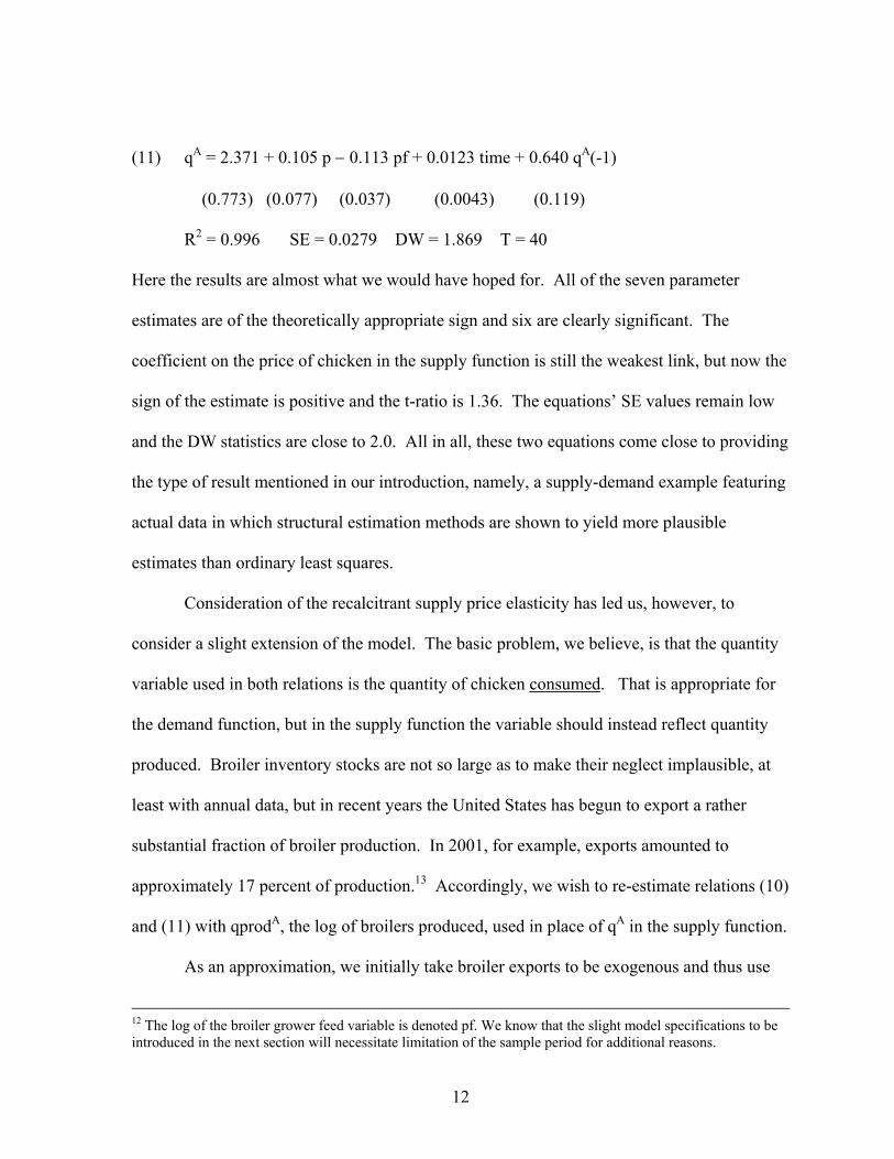
(11) qA = 2.371 + 0.105 p − 0.113 pf + 0.0123 time + 0.640 qA(-1)
(0.773) (0.077) (0.037) (0.0043) (0.119)
R2 = 0.996 SE = 0.0279 DW = 1.869 T = 40
Here the results are almost what we would have hoped for. All of the seven parameter
estimates are of the theoretically appropriate sign and six are clearly significant. The
coefficient on the price of chicken in the supply function is still the weakest link, but now the
sign of the estimate is positive and the t-ratio is 1.36. The equations’ SE values remain low
and the DW statistics are close to 2.0. All in all, these two equations come close to providing
the type of result mentioned in our introduction, namely, a supply-demand example featuring
actual data in which structural estimation methods are shown to yield more plausible
estimates than ordinary least squares.
Consideration of the recalcitrant supply price elasticity has led us, however, to
consider a slight extension of the model. The basic problem, we believe, is that the quantity
variable used in both relations is the quantity of chicken consumed. That is appropriate for
the demand function, but in the supply function the variable should instead reflect quantity
produced. Broiler inventory stocks are not so large as to make their neglect implausible, at
least with annual data, but in recent years the United States has begun to export a rather
substantial fraction of broiler production. In 2001, for example, exports amounted to
approximately 17 percent of production.13 Accordingly, we wish to re-estimate relations (10)
and (11) with qprodA, the log of broilers produced, used in place of qA in the supply function.
As an approximation, we initially take broiler exports to be exogenous and thus use
12 The log of the broiler grower feed variable is denoted pf. We know that the slight model specifications to be introduced in the next section will necessitate limitation of the sample period for additional reasons.
13
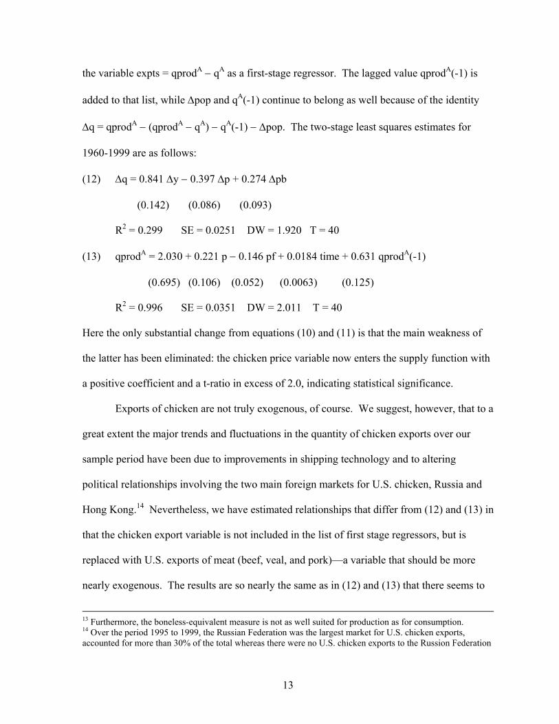
the variable expts = qprodA − qA as a first-stage regressor. The lagged value qprodA(-1) is
added to that list, while ∆pop and qA(-1) continue to belong as well because of the identity
∆q = qprodA − (qprodA − qA) − qA(-1) − ∆pop. The two-stage least squares estimates for
1960-1999 are as follows:
(12) ∆q = 0.841 ∆y − 0.397 ∆p + 0.274 ∆pb
(0.142) (0.086) (0.093)
R2 = 0.299 SE = 0.0251 DW = 1.920 T = 40
(13) qprodA = 2.030 + 0.221 p − 0.146 pf + 0.0184 time + 0.631 qprodA(-1)
(0.695) (0.106) (0.052) (0.0063) (0.125)
R2 = 0.996 SE = 0.0351 DW = 2.011 T = 40
Here the only substantial change from equations (10) and (11) is that the main weakness of
the latter has been eliminated: the chicken price variable now enters the supply function with
a positive coefficient and a t-ratio in excess of 2.0, indicating statistical significance.
Exports of chicken are not truly exogenous, of course. We suggest, however, that to a
great extent the major trends and fluctuations in the quantity of chicken exports over our
sample period have been due to improvements in shipping technology and to altering
political relationships involving the two main foreign markets for U.S. chicken, Russia and
Hong Kong.14 Nevertheless, we have estimated relationships that differ from (12) and (13) in
that the chicken export variable is not included in the list of first stage regressors, but is
replaced with U.S. exports of meat (beef, veal, and pork)—a variable that should be more
nearly exogenous. The results are so nearly the same as in (12) and (13) that there seems to
13 Furthermore, the boneless-equivalent measure is not as well suited for production as for consumption. 14 Over the period 1995 to 1999, the Russian Federation was the largest market for U.S. chicken exports, accounted for more than 30% of the total whereas there were no U.S. chicken exports to the Russion Federation
14
be no point in taking the space to report them.
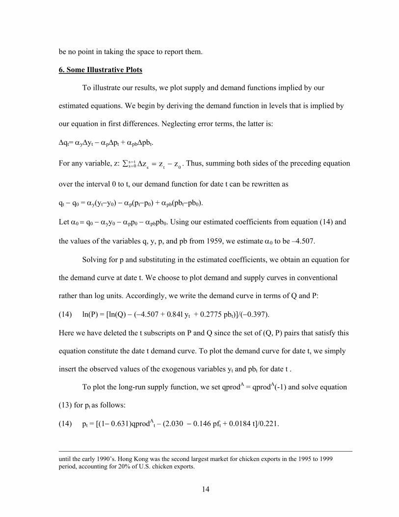
6. Some Illustrative Plots
To illustrate our results, we plot supply and demand functions implied by our
estimated equations. We begin by deriving the demand function in levels that is implied by
our equation in first differences. Neglecting error terms, the latter is:
∆qt= αy∆yt − αp∆pt + αpb∆pbt.
For any variable, z: s ts 0 s t 0z z z==∑ ∆ = − . Thus, summing both sides of the preceding equation
over the interval 0 to t, our demand function for date t can be rewritten as
qt − q0 = αy(yt−y0) − αp(pt−p0) + αpb(pbt−pb0).
Let α0 = q0 − αyy0 − αpp0 − αpbpb0. Using our estimated coefficients from equation (14) and
the values of the variables q, y, p, and pb from 1959, we estimate α0 to be –4.507.
Solving for p and substituting in the estimated coefficients, we obtain an equation for
the demand curve at date t. We choose to plot demand and supply curves in conventional
rather than log units. Accordingly, we write the demand curve in terms of Q and P:
(14) ln(P) = [ln(Q) − (−4.507 + 0.841yt + 0.2775 pbt)]/(−0.397).
Here we have deleted the t subscripts on P and Q since the set of (Q, P) pairs that satisfy this
equation constitute the date t demand curve. To plot the demand curve for date t, we simply
insert the observed values of the exogenous variables yt and pbt for date t .
To plot the long-run supply function, we set qprodA = qprodA(-1) and solve equation
(13) for pt as follows:
(14) pt = [(1− 0.631)qprodAt – (2.030 − 0.146 pft + 0.0184 t]/0.221.
until the early 1990’s. Hong Kong was the second largest market for chicken exports in the 1995 to 1999 period, accounting for 20% of U.S. chicken exports.
15
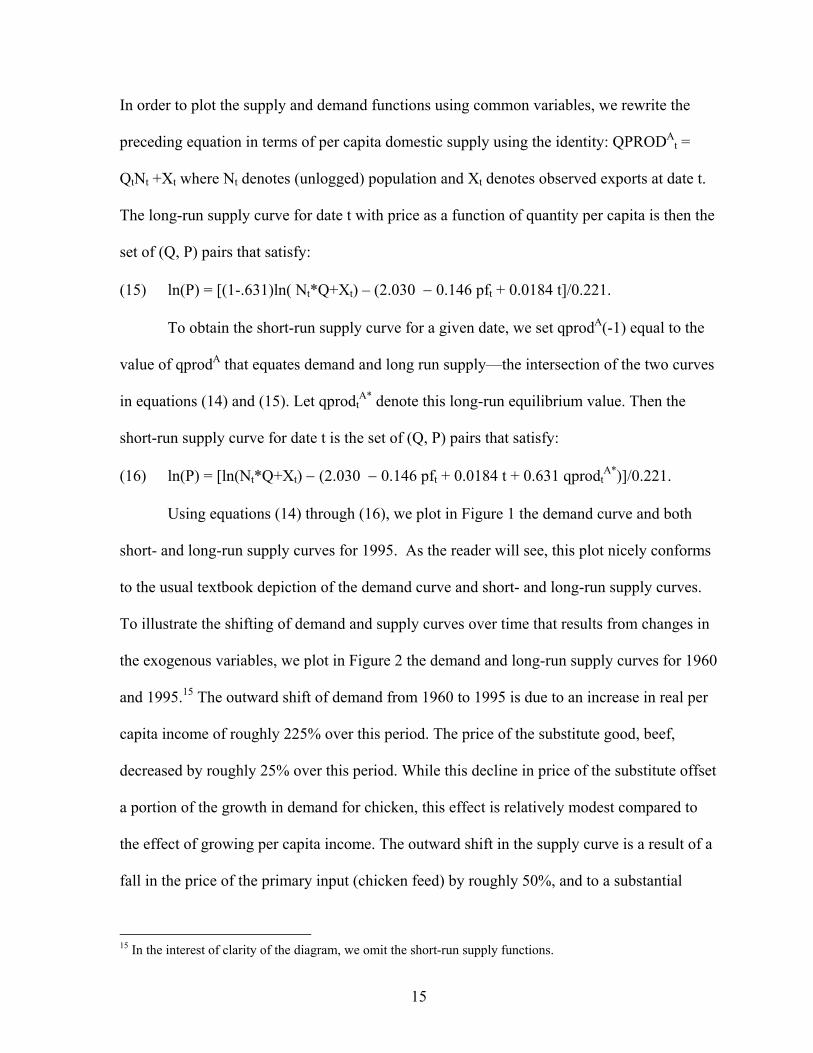
In order to plot the supply and demand functions using common variables, we rewrite the
preceding equation in terms of per capita domestic supply using the identity: QPRODAt =
QtNt +Xt where Nt denotes (unlogged) population and Xt denotes observed exports at date t.
The long-run supply curve for date t with price as a function of quantity per capita is then the
set of (Q, P) pairs that satisfy:
(15) ln(P) = [(1-.631)ln( Nt*Q+Xt) – (2.030 − 0.146 pft + 0.0184 t]/0.221.
To obtain the short-run supply curve for a given date, we set qprodA(-1) equal to the
value of qprodA that equates demand and long run supply—the intersection of the two curves
in equations (14) and (15). Let qprodtA* denote this long-run equilibrium value. Then the
short-run supply curve for date t is the set of (Q, P) pairs that satisfy:
(16) ln(P) = [ln(Nt*Q+Xt) − (2.030 − 0.146 pft + 0.0184 t + 0.631 qprodtA*)]/0.221.
Using equations (14) through (16), we plot in Figure 1 the demand curve and both
short- and long-run supply curves for 1995. As the reader will see, this plot nicely conforms
to the usual textbook depiction of the demand curve and short- and long-run supply curves.
To illustrate the shifting of demand and supply curves over time that results from changes in
the exogenous variables, we plot in Figure 2 the demand and long-run supply curves for 1960
and 1995.15 The outward shift of demand from 1960 to 1995 is due to an increase in real per
capita income of roughly 225% over this period. The price of the substitute good, beef,
decreased by roughly 25% over this period. While this decline in price of the substitute offset
a portion of the growth in demand for chicken, this effect is relatively modest compared to
the effect of growing per capita income. The outward shift in the supply curve is a result of a
fall in the price of the primary input (chicken feed) by roughly 50%, and to a substantial
15 In the interest of clarity of the diagram, we omit the short-run supply functions.

16
0.0
0.5
1.0
1.5
2.0
2.5
0 10 20 30 40 50 60 70 80
QUANTITY
PR
ICE
Demand
Long RunSupply
Short RunSupply
Figure 1
DEMAND AND SUPPLY CURVES, 1995

17
0.0
0.5
1.0
1.5
2.0
2.5
0 10 20 30 40 50 60 70 80
Figure 2
DEMAND AND LONG RUN SUPPLY CURVES1960 AND 1995
1960
1995
QUANTITY
PR
ICE
18
productivity increase in chicken production. The latter is captured by the coefficient of
0.0183 on the time variable in the supply function. As is evident from Figure 2, the outward
shift in supply was more rapid than the outward shift in demand, leading to a substantial fall
in the real price of chicken over the 35-year time interval.16
7. Conclusion
The model in equations (12) and (13) meets the objectives we set forth at the outset.
The estimated demand coefficients imply an own-price elasticity of −0.40, an income
elasticity of 0.84, and a cross-price elasticity with respect to the substitute good (beef) of
0.274. These are of the expected algebraic signs and strike us as being quite reasonable in
magnitude. The short-run own-price elasticity of supply is 0.22, and the short-run elasticity
of supply with respect to the price of the primary input (feed) is −0.15. The corresponding
long-run elasticities are 0.60 and −0.40, respectively. Again, these are of the expected
algebraic signs and seem to be quite plausible in magnitude. The estimates also imply a
substantial rate of growth of productivity in chicken production. In particular, the short-run
supply curves exhibits a shift of 1.84% in each one-year interval, holding constant previous-
year production. The long-run supply curve shifts outward by about 5% per year. This rapid
rate of productivity growth largely accounts for the falling real price of chicken in the face of
the prodigious increase in demand observed over our sample period—an increase of 275% in
consumption per capita coupled with a 50% increase in population. In addition to being of
the correct signs and reasonable magnitudes, all of our coefficient estimates are statistically
significant at the conventional 5% level.
16 While we have plotted our demand and supply curves in per capita terms, it is of interest to note that population increased by almost 50% from 1960 to 1995. Thus the total physical quantities produced and consumed increased by a correspondingly greater proportion than the per capita values shown in our plots.
19
Our results, particularly for the supply equation, also illustrate the payoff from
estimating the equations as a simultaneous system. The single-equation coefficient estimates
for the supply equation (9) yield a supply price elasticity that is of the wrong algebraic sign
and statistically insignificant. By contrast, the supply equation (13) estimated with two-stage
least squares is of the correct sign and statistically significant. This accomplishment of
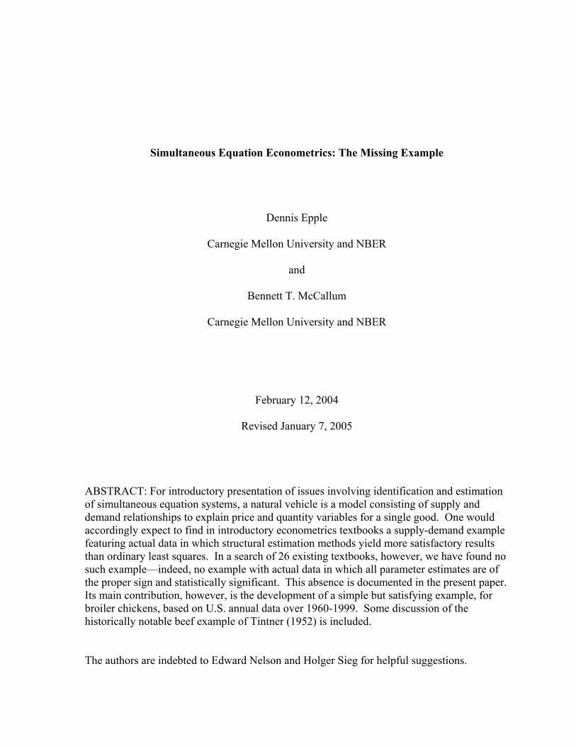
systems estimation is all the more striking when considered in light of the plot of price versus
quantity produced (Figure 3), which exhibits a pronounced inverse relationship between the
two. Despite that strong negative relationship, the systems approach produces an estimated
supply function in which quantity produced is an increasing and statistically significant
function of price.

20
0.9
1.0
1.1
1.2
1.3
1.4
1.5
1.6
1.7
1.8
0 5000 10000 15000 20000 25000
Aggregate Chicken Production
Inde
x of
Rea
l Pric
e of
Chi
cken
Figure 3
Chicken Price and Production, 1960-1999
21
Appendix A
Data from French (1949)
22
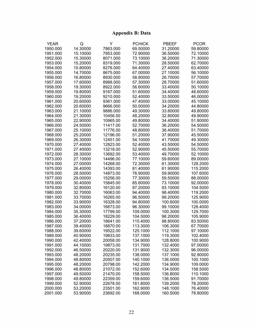
Appendix B: Data
YEAR Q Y PCHICK PBEEF PCOR 1950.000 14.30000 7863.000 69.50000 31.20000 59.80000 1951.000 15.10000 7953.000 72.90000 36.50000 72.10000 1952.000 15.30000 8071.000 73.10000 36.20000 71.30000 1953.000 15.20000 8319.000 71.30000 28.50000 62.70000 1954.000 15.80000 8276.000 64.40000 27.40000 63.40000 1955.000 14.70000 8675.000 67.00000 27.10000 56.10000 1956.000 16.80000 8930.000 58.80000 26.70000 57.70000 1957.000 17.60000 8988.000 57.30000 28.70000 51.60000 1958.000 19.30000 8922.000 56.60000 33.40000 50.10000 1959.000 19.80000 9167.000 51.60000 34.40000 48.60000 1960.000 19.20000 9210.000 52.40000 33.50000 46.00000 1961.000 20.60000 9361.000 47.40000 33.00000 45.10000 1962.000 20.60000 9666.000 50.00000 34.20000 44.80000 1963.000 21.10000 9886.000 49.30000 33.80000 49.80000 1964.000 21.30000 10456.00 48.20000 32.80000 49.90000 1965.000 22.90000 10965.00 49.80000 34.40000 51.80000 1966.000 24.50000 11417.00 52.70000 36.20000 54.50000 1967.000 25.10000 11776.00 48.80000 36.40000 51.70000 1968.000 25.20000 12196.00 51.20000 37.90000 45.50000 1969.000 26.30000 12451.00 54.10000 41.70000 49.30000 1970.000 27.40000 12823.00 52.40000 43.50000 54.50000 1971.000 27.40000 13218.00 52.90000 45.50000 55.70000 1972.000 28.30000 13692.00 53.40000 49.70000 52.10000 1973.000 27.10000 14496.00 77.10000 59.60000 89.00000 1974.000 27.00000 14268.00 72.30000 61.30000 128.2000 1975.000 26.40000 14393.00 81.40000 61.90000 115.2000 1976.000 28.50000 14873.00 76.90000 59.90000 107.6000 1977.000 29.00000 15256.00 77.30000 59.50000 88.00000 1978.000 30.40000 15845.00 85.60000 73.10000 92.00000 1979.000 32.80000 16120.00 87.20000 93.10000 104.5000 1980.000 32.70000 16063.00 94.40000 98.40000 119.2000 1981.000 33.70000 16265.00 96.50000 99.20000 125.9000 1982.000 33.90000 16328.00 94.80000 100.6000 100.0000 1983.000 34.00000 16673.00 96.30000 99.10000 128.4000 1984.000 35.30000 17799.00 109.0000 100.3000 129.7000 1985.000 36.40000 18229.00 104.5000 98.20000 105.9000 1986.000 37.20000 18641.00 115.4000 98.80000 83.50000 1987.000 39.40000 18870.00 113.3000 106.3000 67.70000 1988.000 39.60000 19522.00 125.1000 112.1000 97.10000 1989.000 40.90000 19833.00 137.1000 119.3000 102.4000 1990.000 42.40000 20058.00 134.9000 128.8000 100.9000 1991.000 44.10000 19873.00 131.7000 132.4000 97.00000 1992.000 46.50000 20220.00 131.9000 132.3000 96.00000 1993.000 48.20000 20235.00 138.0000 137.1000 92.90000 1994.000 48.80000 20507.00 140.1000 136.0000 100.1000 1995.000 48.20000 20798.00 142.2000 134.9000 109.0000 1996.000 48.80000 21072.00 152.6000 134.5000 158.5000 1997.000 49.50000 21470.00 158.5000 136.8000 110.1000 1998.000 49.80000 22359.00 159.6000 136.5000 91.70000 1999.000 52.90000 22678.00 161.8000 139.2000 78.20000 2000.000 53.20000 23501.00 162.9000 148.1000 76.40000 2001.000 53.90000 23692.00 168.0000 160.5000 78.80000
23
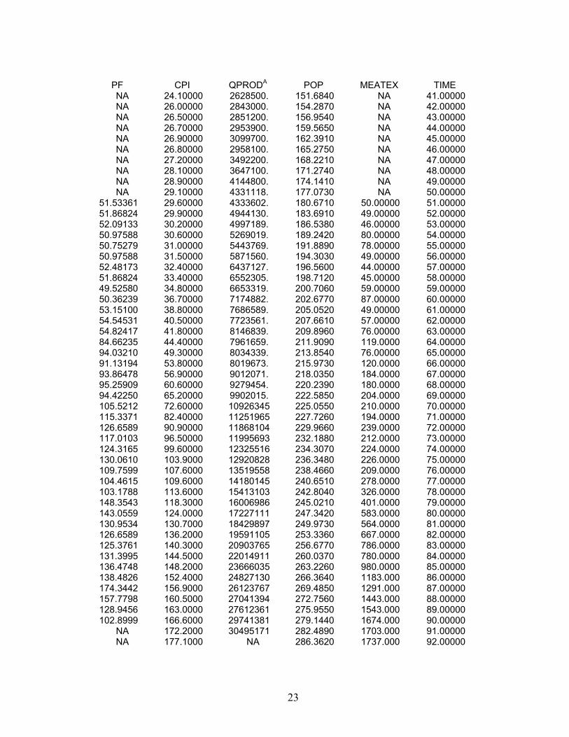
PF CPI QPRODA POP MEATEX TIME
NA 24.10000 2628500. 151.6840 NA 41.00000 NA 26.00000 2843000. 154.2870 NA 42.00000 NA 26.50000 2851200. 156.9540 NA 43.00000 NA 26.70000 2953900. 159.5650 NA 44.00000 NA 26.90000 3099700. 162.3910 NA 45.00000 NA 26.80000 2958100. 165.2750 NA 46.00000 NA 27.20000 3492200. 168.2210 NA 47.00000 NA 28.10000 3647100. 171.2740 NA 48.00000 NA 28.90000 4144800. 174.1410 NA 49.00000 NA 29.10000 4331118. 177.0730 NA 50.00000
51.53361 29.60000 4333602. 180.6710 50.00000 51.00000 51.86824 29.90000 4944130. 183.6910 49.00000 52.00000 52.09133 30.20000 4997189. 186.5380 46.00000 53.00000 50.97588 30.60000 5269019. 189.2420 80.00000 54.00000 50.75279 31.00000 5443769. 191.8890 78.00000 55.00000 50.97588 31.50000 5871560. 194.3030 49.00000 56.00000 52.48173 32.40000 6437127. 196.5600 44.00000 57.00000 51.86824 33.40000 6552305. 198.7120 45.00000 58.00000 49.52580 34.80000 6653319. 200.7060 59.00000 59.00000 50.36239 36.70000 7174882. 202.6770 87.00000 60.00000 53.15100 38.80000 7686589. 205.0520 49.00000 61.00000 54.54531 40.50000 7723561. 207.6610 57.00000 62.00000 54.82417 41.80000 8146839. 209.8960 76.00000 63.00000 84.66235 44.40000 7961659. 211.9090 119.0000 64.00000 94.03210 49.30000 8034339. 213.8540 76.00000 65.00000 91.13194 53.80000 8019673. 215.9730 120.0000 66.00000 93.86478 56.90000 9012071. 218.0350 184.0000 67.00000 95.25909 60.60000 9279454. 220.2390 180.0000 68.00000 94.42250 65.20000 9902015. 222.5850 204.0000 69.00000 105.5212 72.60000 10926345 225.0550 210.0000 70.00000 115.3371 82.40000 11251965 227.7260 194.0000 71.00000 126.6589 90.90000 11868104 229.9660 239.0000 72.00000 117.0103 96.50000 11995693 232.1880 212.0000 73.00000 124.3165 99.60000 12325516 234.3070 224.0000 74.00000 130.0610 103.9000 12920828 236.3480 226.0000 75.00000 109.7599 107.6000 13519558 238.4660 209.0000 76.00000 104.4615 109.6000 14180145 240.6510 278.0000 77.00000 103.1788 113.6000 15413103 242.8040 326.0000 78.00000 148.3543 118.3000 16006986 245.0210 401.0000 79.00000 143.0559 124.0000 17227111 247.3420 583.0000 80.00000 130.9534 130.7000 18429897 249.9730 564.0000 81.00000 126.6589 136.2000 19591105 253.3360 667.0000 82.00000 125.3761 140.3000 20903765 256.6770 786.0000 83.00000 131.3995 144.5000 22014911 260.0370 780.0000 84.00000 136.4748 148.2000 23666035 263.2260 980.0000 85.00000 138.4826 152.4000 24827130 266.3640 1183.000 86.00000 174.3442 156.9000 26123767 269.4850 1291.000 87.00000 157.7798 160.5000 27041394 272.7560 1443.000 88.00000 128.9456 163.0000 27612361 275.9550 1543.000 89.00000 102.8999 166.6000 29741381 279.1440 1674.000 90.00000
NA 172.2000 30495171 282.4890 1703.000 91.00000 NA 177.1000 NA 286.3620 1737.000 92.00000
24
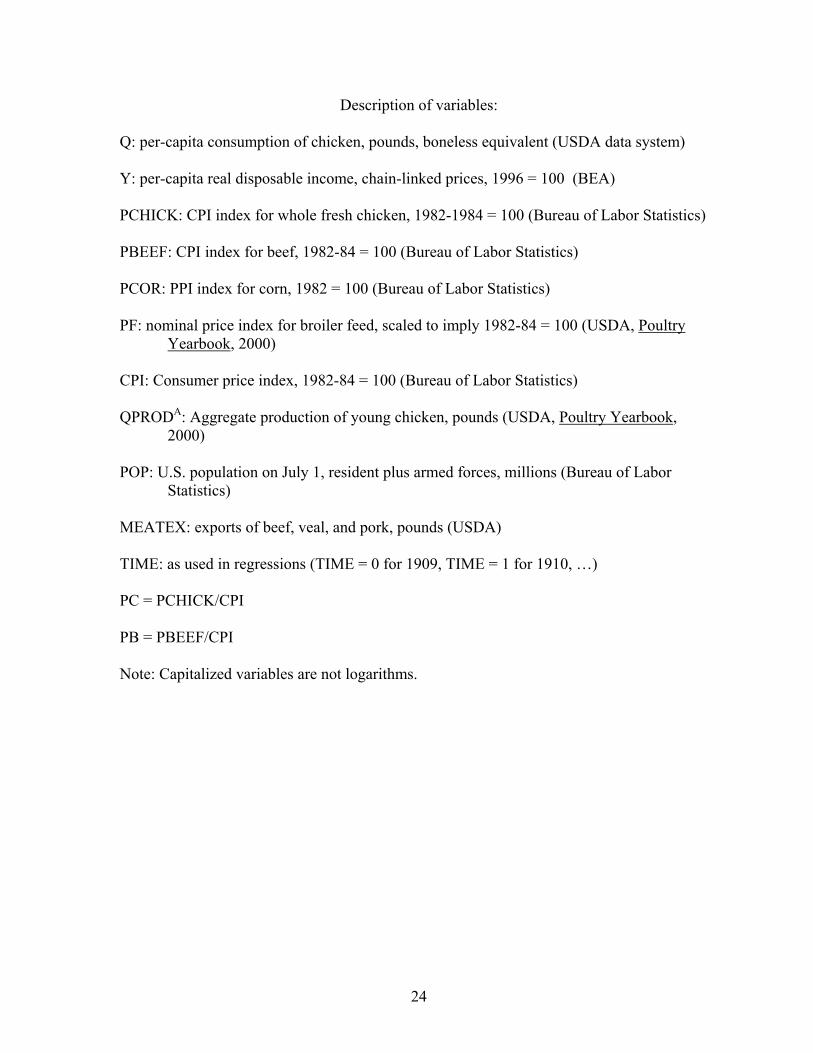
Description of variables:
Q: per-capita consumption of chicken, pounds, boneless equivalent (USDA data system) Y: per-capita real disposable income, chain-linked prices, 1996 = 100 (BEA) PCHICK: CPI index for whole fresh chicken, 1982-1984 = 100 (Bureau of Labor Statistics) PBEEF: CPI index for beef, 1982-84 = 100 (Bureau of Labor Statistics) PCOR: PPI index for corn, 1982 = 100 (Bureau of Labor Statistics) PF: nominal price index for broiler feed, scaled to imply 1982-84 = 100 (USDA, Poultry
Yearbook, 2000)
CPI: Consumer price index, 1982-84 = 100 (Bureau of Labor Statistics) QPRODA: Aggregate production of young chicken, pounds (USDA, Poultry Yearbook,
2000) POP: U.S. population on July 1, resident plus armed forces, millions (Bureau of Labor Statistics) MEATEX: exports of beef, veal, and pork, pounds (USDA) TIME: as used in regressions (TIME = 0 for 1909, TIME = 1 for 1910, …) PC = PCHICK/CPI PB = PBEEF/CPI Note: Capitalized variables are not logarithms.

25
References Ashenfelter, O., P.B. Levine, and D.J. Zimmerman (2003) Statistics and Econometrics:
Methods and Applications. New York: John Wiley.
Beals, R. E. (1972) Statistics for Economists. Chicago: Rand McNally.
Christ, C. F. (1966) Econometric Models and Methods. New York: John Wiley
Frank, C. R. (1971) Statistics and Econometrics. New York: Holt, Rinehart, and Winston.
French, B. L. (1949) Application of Simultaneous Equations to the Analysis of the Demand
for Meat. MS Thesis, Iowa State College.
Goldberger, A. S. (1964) Econometric Theory. New York: John Wiley.
Gujarati, D. N. (1995) Basic Econometrics, 3rd ed. New York: McGraw-Hill.
Haavelmo, T. (1943) “The Statistical Implications of a System of Simultaneous Equations,”
Econometrica 11, 1-12.
__________. (1944) “The Probability Approach in Econometrics,” Econometrica 12
Supplement, 118 pages.
Hausman, J. A. (1983) “Specification and Estimation of Simultaneous Equation Models,”
Handbook of Econometrics, vol.1, Z. Griliches and M. D. Intriligator, eds.
Amsterdam: Elsevier Science.
Hill, R. C., W. E. Griffiths, and G. G. Judge (2000) Undergraduate Econometrics, 2nd ed.
New York: John Wiley.
Johnston, J. (1963) Econometric Methods. New York: McGraw-Hill.
Johnston, J., and J. DiNardo (1997) Econometric Methods, 4th ed. New York: McGraw-Hill.
Kelejian, H. H., and W. E. Oates (1974) Introduction to Econometrics. New York: Harper &
Row.
26
Kennedy, (1979) A Guide to Econometrics. Cambridge, MA: MIT Press
Klein, L. R. (1953) A Textbook of Econometrics. Evanston: Row, Peterson
_________. (1962) An Introduction to Econometrics. Englewood Cliffs: Prentice-Hall.
Kmenta, J. (1971) Elements of Econometrics. New York: Macmillan.
Maddala, G. S. (1977) Econometrics. New York: McGraw-Hill.
__________. (1992) Introduction to Econometrics. Englewood Cliffs: Prentice-Hall.
Malinvaud, E. (1966) Statistical Methods of Econometrics. Chicago: Rand McNally
Merrill, W. C., and K. A. Fox (1970) Introduction to Economic Statistics. New York:
John Wiley.
Murphy, J. L. (1973) Introductory Econometrics. Homewood, IL: Irwin.
Pindyck, R. S., and D. L. Rubinfeld (1976) Econometric Models and Economic Forecasts.
New York: McGraw-Hill.
Schmidt, S.J. (2004) Econometrics. New York: McGraw-Hill/Irwin.
Theil, H. (1971) Principles of Econometrics. New York: John Wiley.
Tintner, G. (1952) Econometrics. New York: John Wiley.
Valavanis, S. (1959) Econometrics. New York: McGraw-Hill.
Wallace and Silver (1988) Econometrics: An Introduction. Reading, MA: Addison-Wesley.
Wooldridge, J. M. (2003) Econometrics: A Modern Approach, 2nd ed. Mason, OH:
Southwestern .
Wonnacott, R. J., and T. H. Wonnacott (1970) Econometrics. New York: John Wiley.
Related Documents