Simulator of the JET real-time disruption predictor - Archivo ...

Simulator of the JET real-time disruption predictor

J.M. Lopez*, S. Dormido-Canto, J. Vega, A. Murari, J.M. Ramirez, M.Ruiz, G. de Arcas and JET-EFDA Contributors*CAEND, Universidad Politecnica de Madrid

7th Workshop on Fusion Data Processing Validation and Analysis, March 27, 2012

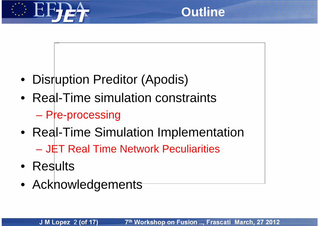
Outline

• Disruption Preditor (Apodis)• Real-Time simulation constraints

– Pre-processing• Real-Time Simulation Implementation

– JET Real Time Network Peculiarities

• Results• Acknowledgements

Focus

• Disruption in tokamaks devices are unavoidable and can have catastrophic effects. So it is very important to have mechanisms to predict this phenomenon.

• These mechanisms have to be:– Accurate and reliable

• High success rate• Low false alarms

– With enough time in advance

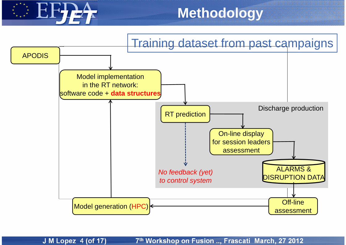
Methodology

ALARMS &DISRUPTION DATA

APODIS

Model implementationin the RT network:

software code + data structures

On-line displayfor session leaders

assessment

Off-lineassessmentModel generation (HPC)

No feedback (yet)to control system

RT predictionDischarge production

Training dataset from past campaigns

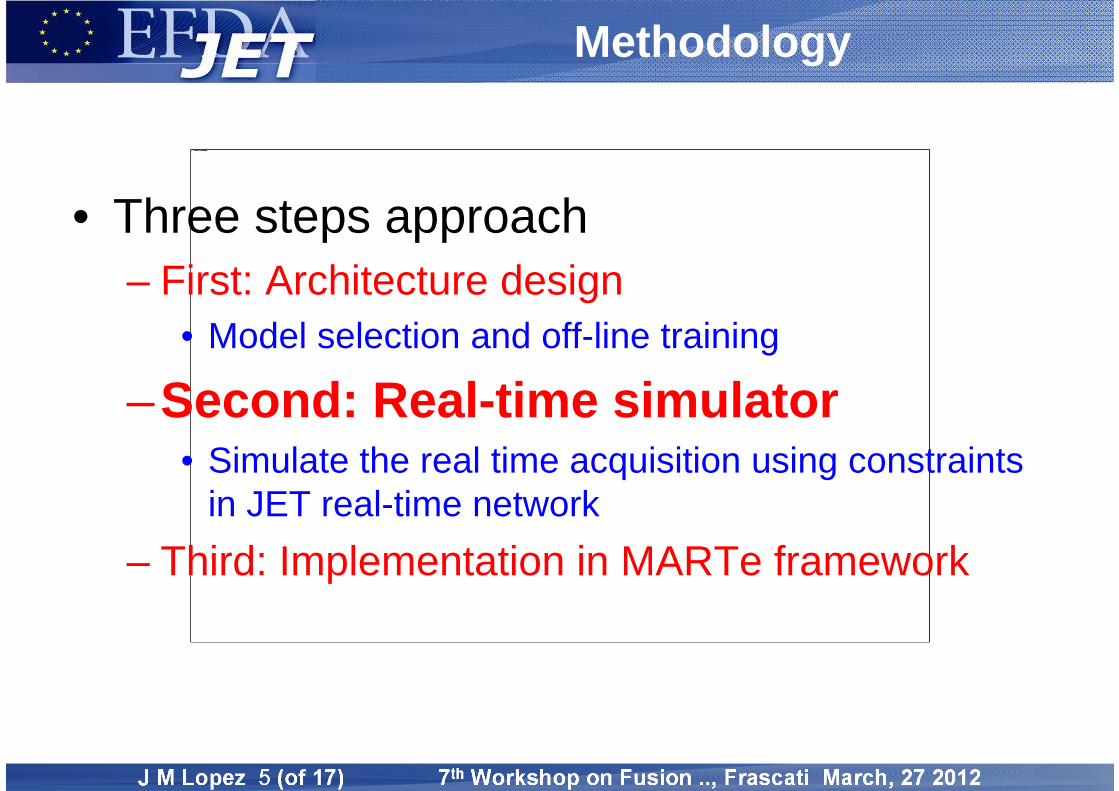
Methodology

• Three steps approach– First: Architecture design

• Model selection and off-line training

–Second: Real-time simulator• Simulate the real time acquisition using constraints

in JET real-time network– Third: Implementation in MARTe framework

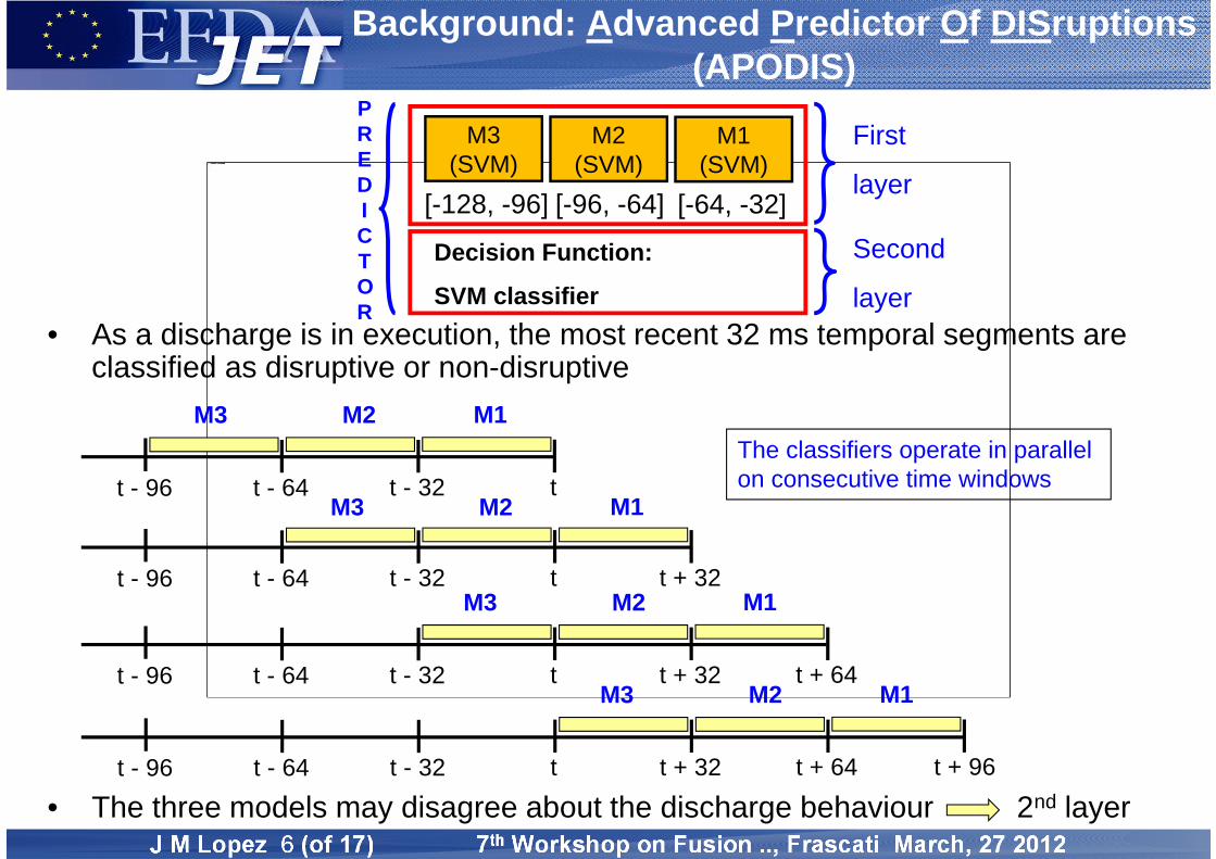
Background: Advanced Predictor Of DISruptions (APODIS)

• As a discharge is in execution, the most recent 32 ms temporal segments are classified as disruptive or non-disruptive

• The three models may disagree about the discharge behaviour 2nd layer

tt - 32t - 64t - 96

M1M2M3

t + 32tt - 32t - 64t - 96

M1M2M3

t + 64t + 32tt - 32t - 64t - 96

M1M2M3

t + 96t + 64t + 32tt - 32t - 64t - 96

M1M2M3

The classifiers operate in parallel on consecutive time windows

PREDICTOR

First

layer

Second

layer

Decision Function:

SVM classifier

[-64, -32][-96, -64][-128, -96]

M1(SVM)

M2(SVM)

M3(SVM)

Background: Advanced Predictor Of DISruptions (APODIS)

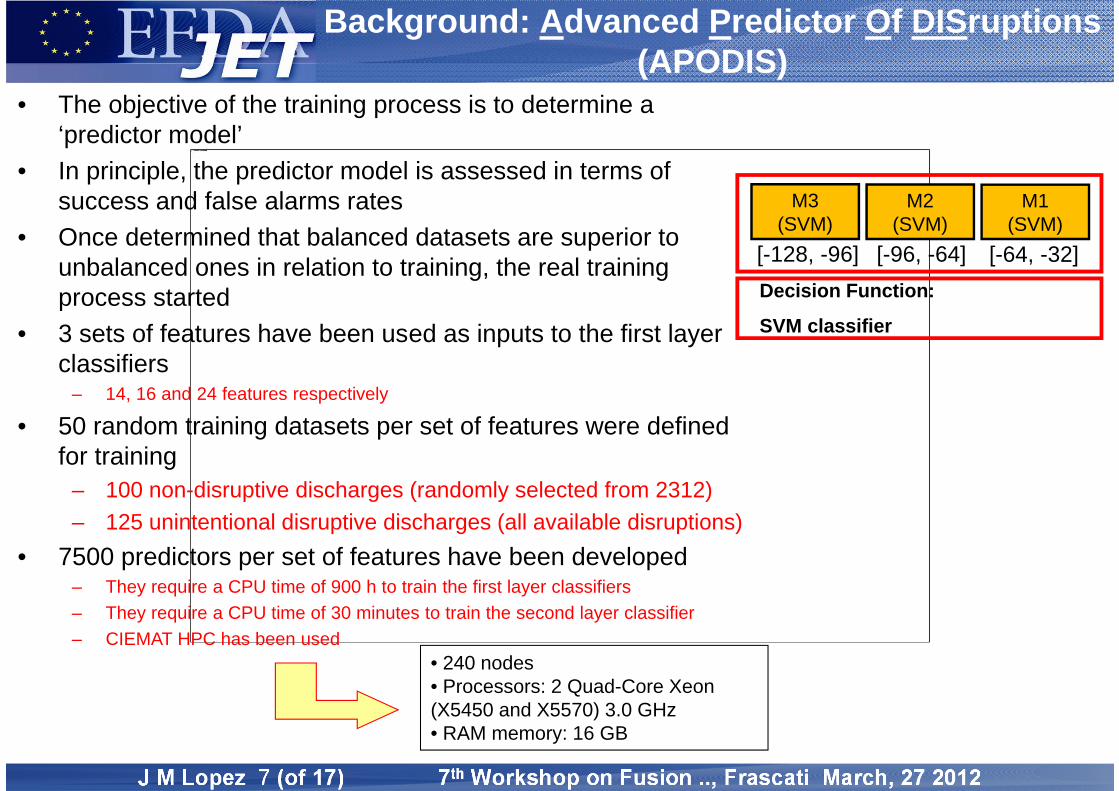
• The objective of the training process is to determine a ‘predictor model’

• In principle, the predictor model is assessed in terms of success and false alarms rates

• Once determined that balanced datasets are superior to unbalanced ones in relation to training, the real training process started

• 3 sets of features have been used as inputs to the first layer classifiers

– 14, 16 and 24 features respectively

• 50 random training datasets per set of features were defined for training

– 100 non-disruptive discharges (randomly selected from 2312)– 125 unintentional disruptive discharges (all available disruptions)

• 7500 predictors per set of features have been developed– They require a CPU time of 900 h to train the first layer classifiers– They require a CPU time of 30 minutes to train the second layer classifier– CIEMAT HPC has been used

Decision Function:

SVM classifier

[-64, -32][-96, -64][-128, -96]

M1(SVM)

M2(SVM)

M3(SVM)

• 240 nodes• Processors: 2 Quad-Core Xeon (X5450 and X5570) 3.0 GHz• RAM memory: 16 GB

Background: Advanced Predictor Of DISruptions (APODIS)

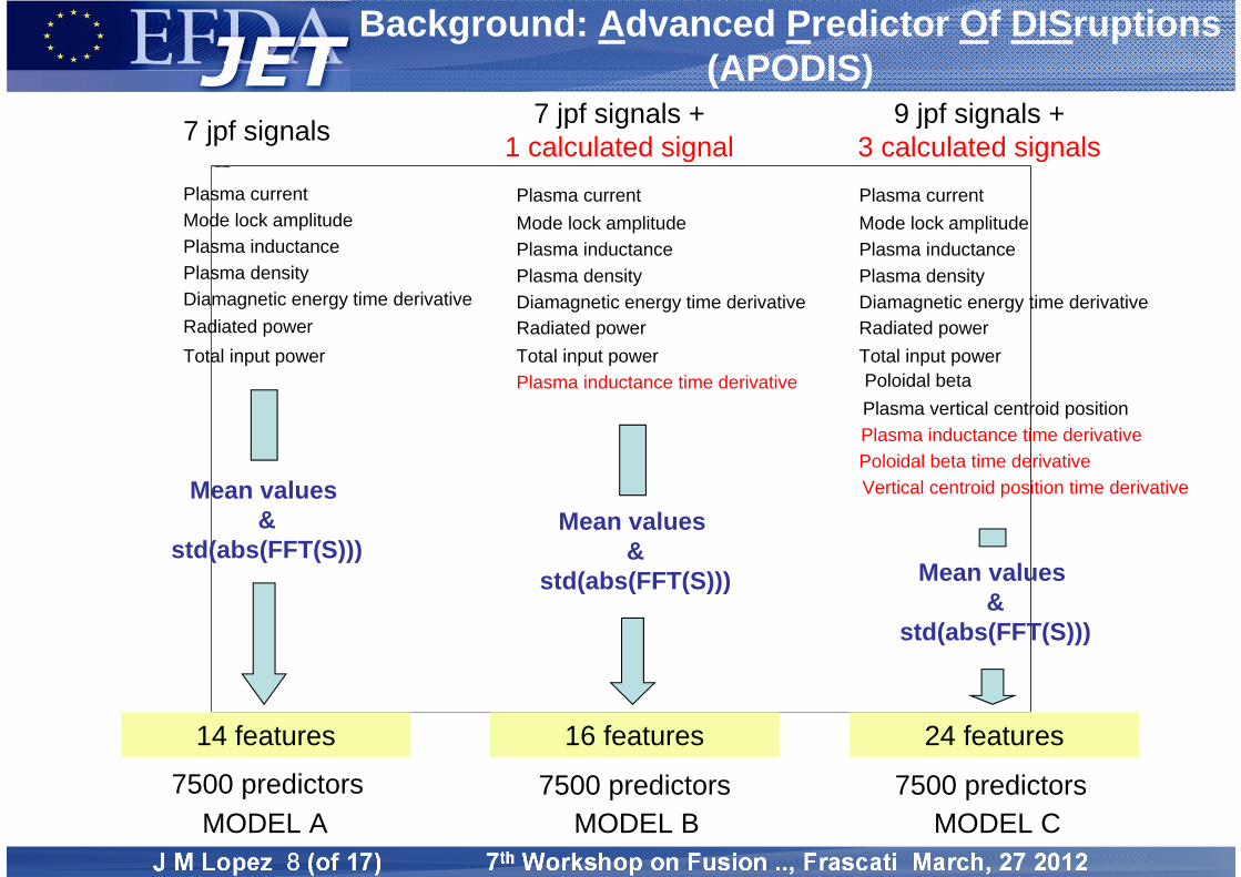
7 jpf signals

Plasma currentMode lock amplitudePlasma inductancePlasma densityDiamagnetic energy time derivativeRadiated powerTotal input power

7 jpf signals +1 calculated signal

Plasma currentMode lock amplitudePlasma inductancePlasma densityDiamagnetic energy time derivativeRadiated powerTotal input powerPlasma inductance time derivative

9 jpf signals +3 calculated signals

Poloidal betaPlasma vertical centroid positionPlasma inductance time derivativePoloidal beta time derivativeVertical centroid position time derivative

MODEL A MODEL B MODEL C

Plasma currentMode lock amplitudePlasma inductancePlasma densityDiamagnetic energy time derivativeRadiated powerTotal input power

Mean values &

std(abs(FFT(S)))

14 features

Mean values &

std(abs(FFT(S)))

16 features

Mean values &

std(abs(FFT(S)))

24 features

7500 predictors 7500 predictors 7500 predictors

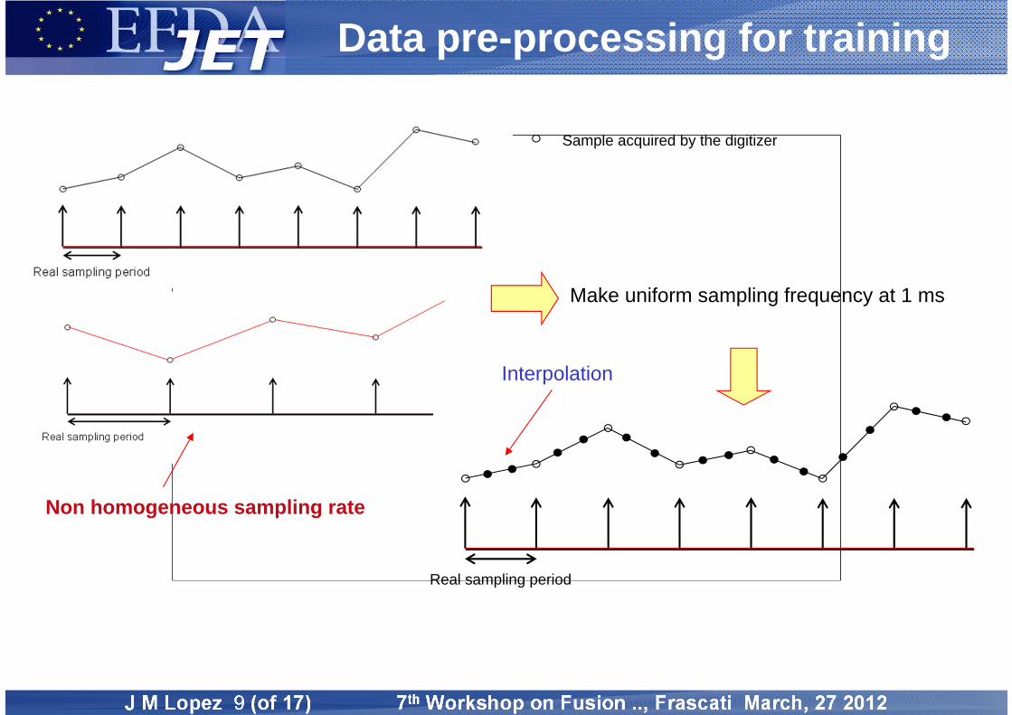
Data pre-processing for training

Make uniform sampling frequency at 1 ms

Sample acquired by the digitizer

Real sampling period

Interpolation

Non homogeneous sampling rate

Data pre-processing for training

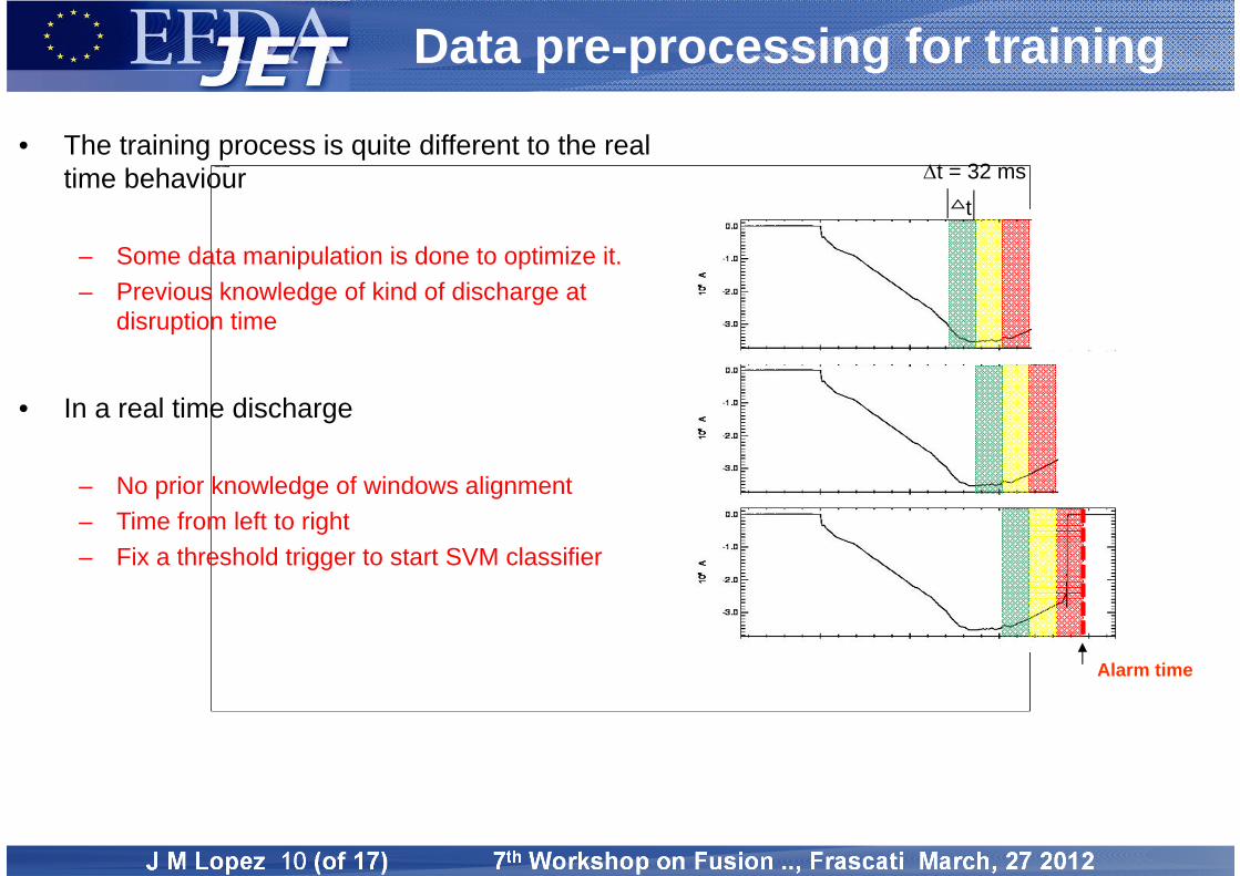
• In a real time discharge

– No prior knowledge of windows alignment– Time from left to right– Fix a threshold trigger to start SVM classifier

Alarm time

t

t = 32 ms• The training process is quite different to the real

time behaviour

– Some data manipulation is done to optimize it.– Previous knowledge of kind of discharge at

disruption time

Real-time Simulator

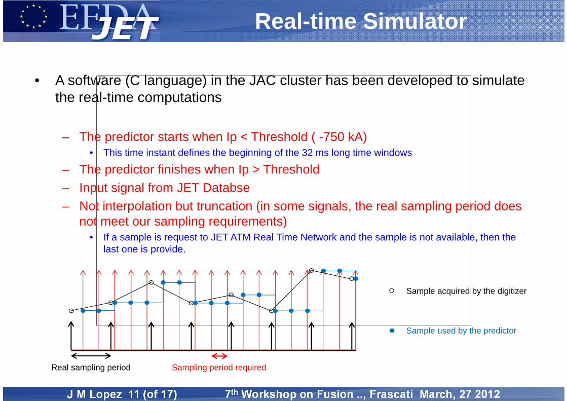
• A software (C language) in the JAC cluster has been developed to simulate the real-time computations

– The predictor starts when Ip < Threshold ( -750 kA)• This time instant defines the beginning of the 32 ms long time windows

– The predictor finishes when Ip > Threshold– Input signal from JET Databse – Not interpolation but truncation (in some signals, the real sampling period does

not meet our sampling requirements)• If a sample is request to JET ATM Real Time Network and the sample is not available, then the

last one is provide.

Real sampling period Sampling period required

Sample acquired by the digitizer

Sample used by the predictor

Real-time Simulator

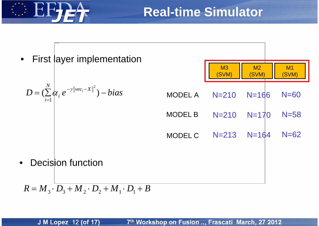
• First layer implementation

biaseD Xveci

N

i

i

)(

2

1

• Decision function

BDMDMDMR 112233

MODEL A

MODEL B

MODEL C

M1(SVM)

M2(SVM)

M3(SVM)

N=60N=166N=210

N=58N=170N=210

N=62N=164N=213

Real-time Simulator

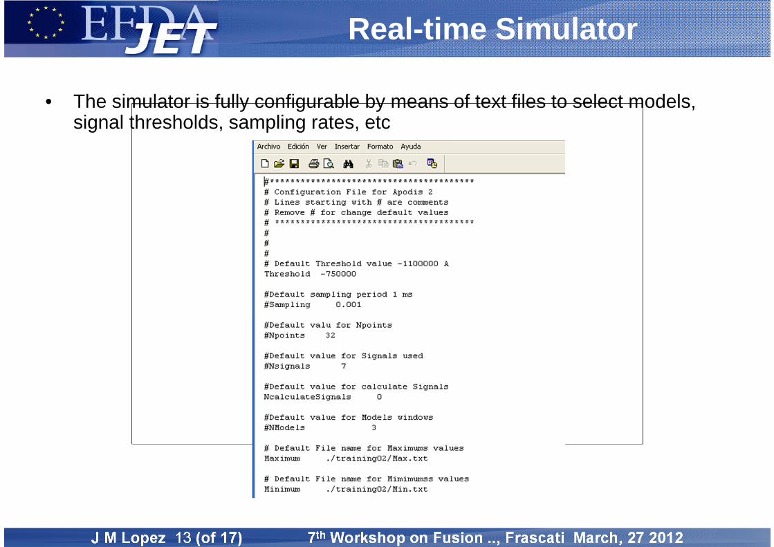
• The simulator is fully configurable by means of text files to select models, signal thresholds, sampling rates, etc

C28 (jpf + ppf) and RT simulation

10-3 10-2 10-1 100 1010

10

20

30

40

50

60

70

80

90

100Campaign: C28

Disruption time - Alarm time [s]

Acc

umul

ativ

e fra

ctio

n of

det

ecte

d di

srup

tions

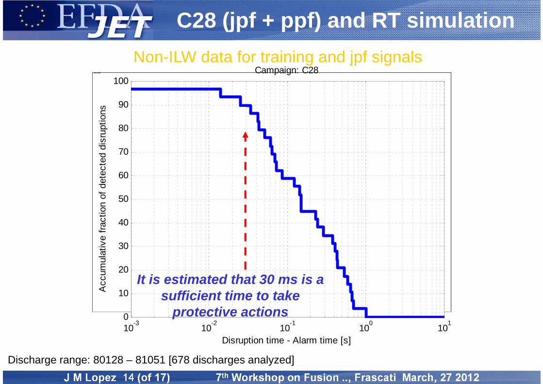
It is estimated that 30 ms is a sufficient time to take

protective actions

Non-ILW data for training and jpf signals

Discharge range: 80128 – 81051 [678 discharges analyzed]

Sumary

• Tool to test Apodis results using JET Database– Works with data files– User configurable – Can work in background mode (Script )

• Simulate the JET ATM Real Time Network behavior

• Model validation before use the real time application under MARTe framework

• The results are equal that obtained in training phase.

Acknowledgements

• We would like to thank in particular:– P. de Vries for the help with the database– D. Alves and R. Felton for the support with

implementation details in ATM Real Time Network

Thank you very much

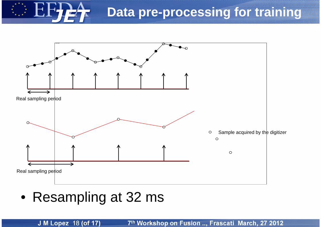
Data pre-processing for training

• Resampling at 32 ms

Real sampling period

Sample acquired by the digitizer

Real sampling period

• Backup

Data pre-processing for training

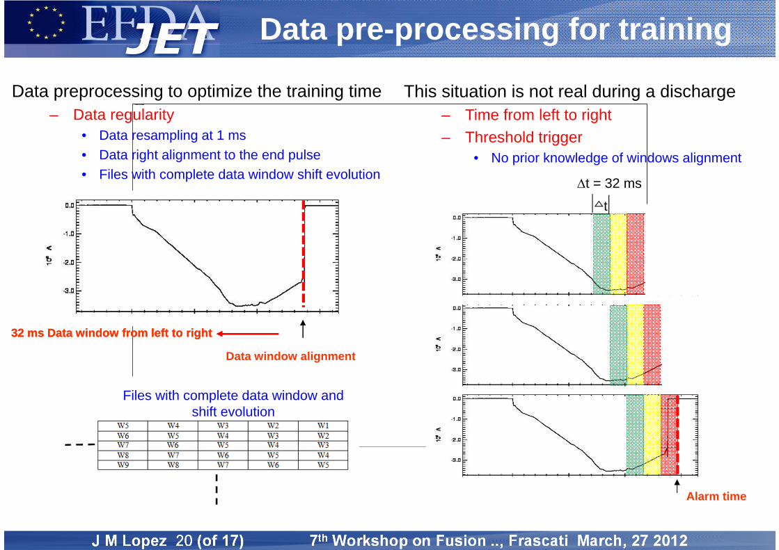
This situation is not real during a discharge– Time from left to right– Threshold trigger

• No prior knowledge of windows alignment

Data window alignment

32 ms Data window from left to right32 ms Data window from left to right

Alarm time

t

t = 32 ms

Data preprocessing to optimize the training time– Data regularity

• Data resampling at 1 ms • Data right alignment to the end pulse• Files with complete data window shift evolution

Files with complete data window and shift evolution