Simulations of the Poynting-Robertson Cosmic Battery in Resistive Accretion Disks

arX

iv:0

706.

3187

v1 [

astr

o-ph

] 1

3 Ju

n 20

07

Simulations of the Poynting–Robertson Cosmic Battery

in Resistive Accretion Disks

Dimitris M. Christodoulou,1 Ioannis Contopoulos,2 and Demosthenes Kazanas3

ABSTRACT

We describe the results of numerical “2.5–dimensional” MHD simulations of

an initially unmagnetized disk model orbiting a central point–mass and respond-

ing to the continual generation of poloidal magnetic field due to a secular source

that emulates the Poynting–Robertson (PR) drag on electrons in the vicinity of

a luminous stellar or compact accreting object. The fluid in the disk and in the

surrounding hotter atmosphere has finite electrical conductivity and allows for

the magnetic field to diffuse freely out of the areas where it is generated, while at

the same time, the differential rotation of the disk twists the poloidal field and

quickly induces a substantial toroidal–field component. The secular PR term has

dual purpose in these simulations as the source of the magnetic field and the trig-

ger of a magnetorotational instability (MRI) in the disk. The MRI is especially

mild and does not destroy the disk because a small amount of resistivity damp-

ens the instability efficiently. In simulations with moderate resistivities (diffusion

timescales up to ∼16 local dynamical times) and after ∼100 orbits, the MRI has

managed to transfer outward substantial amounts of angular momentum and the

inner edge of the disk, along with azimuthal magnetic flux, has flowed toward

the central point–mass where a new, magnetized, nuclear disk has formed. The

toroidal field in this nuclear disk is amplified by differential rotation and it can-

not be contained; when it approaches equipartition, it unwinds vertically and

produces episodic jet–like outflows. The poloidal field in the inner region cannot

diffuse back out if the characteristic diffusion time is of the order of or larger than

the dynamical time; it continues to grow linearly in time undisturbed and without

saturation, as the outer sections of many poloidal loops are being drawn radially

outward by the outflowing matter of high specific angular momentum. On the

other hand, in simulations with low resistivities (diffusion timescales larger than

1Math Methods, 54 Middlesex Turnpike, Bedford, MA 01730. E-mail: [email protected]

2Research Center for Astronomy, Academy of Athens, GR–11527 Athens, Greece.

Email: [email protected]

3NASA/GSFC, Code 663, Greenbelt, MD 20771. E-mail: [email protected]

– 2 –

∼16 local dynamical times), the inflowing matter does not form a nuclear disk

or jets and the linear growth of the poloidal magnetic field is interrupted after

about 20 orbits because of magnetic reconnection and asymmetric outflows.

Subject headings: accretion, accretion disks—instabilities—magnetic fields—

MHD—plasmas

1. Introduction

We revisit the theory of cosmic magnetic field generation via the Poynting–Robertson

(hereafter PR) battery in the vicinity of accretion–powered objects, a process that has been

proposed as a generic means of generating magnetic fields in a variety of astrophysical sites.

The principles of the PR battery have been enunciated by Contopoulos & Kazanas (1998)

and then elaborated by Contopoulos, Kazanas & Christodoulou (2006) (hereafter CK and

CKC, respectively). As was pointed out in CKC, the problem of the origin of cosmic mag-

netic fields is largely of topological nature since the initial conditions of a homogeneous and

isotropic universe allow only for irrotational perturbations to exist. It was also pointed out

in the same reference that the vorticity ω = ∇× v of a velocity field v is subject to

similar constraints and obeys evolution equations identical to those of the magnetic field

(Kulsrud et al. 1997). Since vorticity can only be generated by the action of dissipative

processes (Kelvin’s theorem), it is not unreasonable to also look for generation and growth

of magnetic fields in sites that involve both vorticity and dissipation, such as the accretion

disks considered by CK and CKC.

The question of the source of cosmic magnetic fields has been vexing and it is believed

to still be open to investigation. It is generally thought that small fields (of the order

of 10−20 G) generated by the Biermann (1950) battery could be amplified exponentially by

dynamo processes to match the observed values of ≃ 10−6 G of the interstellar magnetic field

in the Galaxy (Kulsrud et al. 1997). But it has also been pointed out by Vainshtein & Rosner

(1991) that turbulent dynamos can amplify fields to equipartition only on small scales, while

the large–scale field will remain well below equipartition, in apparent disagreement with the

observations (for simulations that support this point, see Fleming, Stone, & Hawley [2000]

and references therein; but see also Igumenshchev, Narayan, & Abramowicz [2003] for recent

developments concerning the evolution of the poloidal field). These arguments rest on the

assumptions that there are no large–scale flows on top of the turbulent motions and that

there are no other sources of magnetic field. In contrast, the PR effect in accreting systems

involves two qualitatively different ingredients: a large–scale organized flow, namely the

inflow that provides the accreting matter onto the compact or stellar object; and a large–

– 3 –

scale continuous source of azimuthal electric current (or, equivalently, a toroidal electric

field). It is our contention that these ingredients can lead to magnetic–field evolution that is

qualitatively very different than that envisioned in small–scale turbulent environments and

thus the PR–battery mechanism can be a better candidate for generating and amplifying

magnetic fields than the Biermann (1950) process and the turbulent dynamo criticized by

Vainshtein & Rosner (1991).

While it is apparent that an azimuthal current such as that of the PR battery would

lead to the generation of poloidal magnetic field, it is not immediately obvious that such a

field is necessarily of significance and some explanations are in order:

1. Although the PR current is quite robust, especially in optically thin accretion disks of

the ADAF type (Narayan & Yi 1994), in one dynamical time it yields magnetic fields

well below equipartition values. But it was pointed out by CK that the importance of

this effect lies in its secular nature: the poloidal field will be amplified by the continual

accumulation of magnetic flux onto the central object due to the persistent large–scale

velocity field and its magnitude will eventually reach dynamically significant levels.

2. The PR current generates naturally only closed poloidal loops. The influx of an en-

tire loop would amplify the central magnetic field for just one typical accretion time

to a value much too small to be of consequence (Bisnovatyi-Kogan & Blinnikov 1977;

Bisnovatyi-Kogan et al. 2002). But it was noted by CK and was demonstrated ex-

plicitly by CKC that the possibility of accumulating a nonzero net magnetic flux in

the central region depends heavily on the rate of inward–advected flux and the rate

of outward diffusion. Specifically, it was shown that a sufficiently high value of the

magnetic diffusivity could help the outer sections of complete poloidal loops escape

outward while the inner sections would still be drawn inward by the inflow, leading to

a secular net increase in central magnetic flux.

The work of CK and CKC shows that there exists a critical dimensionless parameter that

specifies the boundary between different large–scale, long–term behaviors. This parameter

is the inverse1 magnetic Prandtl number (Pm)−1, i.e., the ratio η/ν of magnetic diffusivity

to turbulent kinematic viscosity, a number that is effectively determined by the ratio of the

1CK defined the magnetic Prandtl number as η/ν (the ratio of magnetic diffusivity to turbulent kinematic

viscosity), which is the inverse of what is commonly used in the literature. Since most readers are familiar with

the common definition Pm ≡ ν/η, confusion can be avoided if we heretofore refer to the critical parameter

of CK as (Pm)−1. Field amplification then occurs for (Pm)−1 >∼ 2 according to CK or, equivalently, for

Pm<∼ 0.5.

– 4 –

viscous to the diffusion timescale τvis/τdiff in the disk’s plasma. For (Pm)−1 >∼ 2 (or τvis>∼

2τdiff), the outer section of each loop escapes radially out as discussed above, and the magnetic

flux in the vicinity of the central object increases linearly in time and without bound. On the

other hand, the central magnetic flux quickly reaches saturation to dynamically insignificant

levels in the opposite limit of τvis/τdiff < 2.

The purpose of this work is to study numerically and in greater detail the PR–battery

mechanism and to explore whether the basic premises outlined above can withstand the

scrutiny of such a treatment; and whether the scalings and behavior obtained in our earlier

simplified calculations carry over to detailed multidimensional MHD simulations. To this

end, we have decided to dispense with the viscous prescription of the accretion disk and opted

instead to employ the magnetorotational instability (hereafter MRI) (Balbus & Hawley 1991,

1998) as a means of establishing a global accretion flow from a rotating disk toward the central

object. Our global accretion scenario begins with an initially unmagnetized, geometrically

thick torus embedded into a hotter, nonrotating atmosphere and orbiting a gravitationally–

dominant, central point–mass. The magnetic field is produced continually by a secular source

term that emulates a toroidal electric field due to the PR drag acting predominantly on the

electrons. The fluid in the disk and in the surrounding atmosphere is electrically conducting

and allows for magnetic dissipation to take place on a prescribed diffusion timescale.

The effects that we are interested in are the large–scale response of the fluid in the disk

and the global evolution of the magnetic field. These effects are nonperiodic and nonlocal

and they cannot be studied by using a local approximation such as the “shearing box”

with field diffusion (e.g., Fleming, Stone, & Hawley 2000; Fleming & Stone 2003). More

specifically, the main questions that we wish to investigate concern the fate of the gas and

the magnetic field that are driven from the accretion disk toward the central point–mass

by the MRI and by the process of magnetic diffusion. We know from previous work on the

applicable conservation laws in magnetized fluids (Christodoulou, Contopoulos, & Kazanas

1996, 2003) that azimuthal magnetic flux will also inflow from the accretion disk as some

of the angular momentum will be driven to larger radii. This azimuthal flux along with

gas depleted of its angular momentum will have to accumulate in the vicinity of the central

point–mass. The gas that falls into the nuclear region becomes effectively trapped deeper

into the gravitational potential well of the central object, but the toroidal magnetic field

cannot be trapped as easily, since it has at least two ways out of the nucleus: it can dissipate

if the resistivity of the fluid is high enough; or it can unwind vertically and expel matter in

an axial (possibly bipolar) outflow if the nuclear azimuthal flux grows to a sufficiently large

value (Contopoulos 1995). In addition to the study of the growth and evolution of magnetic

fields in accretion disks which constitutes our main goal, this work also provides some insight

about the influence of resistive effects to the global dynamics of such disks and, in particular,

– 5 –

about the possibilities of MRI suppression and jet formation in the presence of anomalous

resistivity. To the best of our knowledge, the question of how the anomalous resistivity

influences the dynamics of the accreted matter has not yet been explored to sufficient depth.

The remainder of the paper is organized as follows: In § 2, we present the MHD equations

that we solve numerically. These equations include resistive and dissipative effects in the

magnetic field and a source of poloidal field that emulates the effect of an azimuthal electric

current produced by the PR drag operating on electrons in the area around a central object.

In § 3, we discuss the numerical techniques that we use and we describe our initial disk model

and the surrounding isothermal atmosphere in equilibrium around the central point–mass.

In § 4, we describe the most important highlights from our model simulations. Finally, in

§ 5, we discuss the results of the simulations and their significance for astrophysical accretion

disks.

2. The MHD Equations with Resistivity and PR Drag

The MHD equations that we use are subject to the following conditions:

1. The fluid and the magnetic field extend in all three spatial dimensions which are

described in an inertial frame of reference in cylindrical coordinates (R, φ, Z).

2. The fluid is perfect (it has no internal molecular viscosity) and ideal with adiabatic

exponent γ.

3. The fluid is electrically conducting and the electrical conductivity σ can be finite (fields

with ohmic dissipation) or infinite (“frozen–in” fields).

4. The fluid is not self–gravitating but it is influenced by the gravitational field of a central

point–mass M .

5. There exists a source of poloidal magnetic field S = (SR, 0, SZ) due to a toroidal electric

field produced by PR drag.

6. The displacement current is ignored in Amprere’s law.

The system of equations is parameterized by the adiabatic exponent γ, the resistivity η

(which is inversely proportional to the electrical conductivity σ), and by the external sources

of the gravitational field Φ and the poloidal magnetic field S. The parameters γ and η are

both taken to be constant in space and time independent. Gaussian cgs units are chosen, in

– 6 –

which case η = c2/(4πσ), where c is the speed of light. The fundamental MHD variables are

the mass density ρ, the entropy density ǫ, and the momentum density vector M = (MR,

Mφ, MZ) of the fluid, as well as the magnetic field vector B = (BR, Bφ, BZ). Additional

derived variables are the components of the velocity vector v = (vR, vφ, vZ) = (MR/ρ,

Mφ/(ρR), MZ/ρ), the angular velocity in the Z–direction Ω = vφ/R and the corresponding

specific angular momentum L = Rvφ, the internal energy density u = ǫγ , the internal fluid

pressure Pfl = (γ − 1)u, and the electric current density vector J ≡ (c/4π)∇× B.

Under the above conditions, we can write the MHD equations in conservative form as

follows:

The continuity equation expresses mass conservation:

∂ρ

∂t+ ∇·(ρv) = 0 , (1)

where t denotes time and ∇ is the usual del operator.

The components of the momentum equation describe the transfer of momentum within

the fluid:

∂MR

∂t+ ∇·(MRv) = − ∂

∂R

(

Pfl +B2

8π

)

− ρ∂Φ

∂R+

ρv2φ

R+

1

4π(B · ∇)BR , (2)

∂Mφ

∂t+ ∇·(Mφv) = − ∂

∂φ

(

Pfl +B2

8π

)

− ρ∂Φ

∂φ+

R

4π(B · ∇)Bφ , (3)

∂MZ

∂t+ ∇·(MZv) = − ∂

∂Z

(

Pfl +B2

8π

)

− ρ∂Φ

∂Z+

1

4π(B · ∇)BZ . (4)

In these three equations, the components of the usual Lorentz acceleration (∇×B) × B/4π

have been split into two terms, the gradient of the magnetic pressure Pmag ≡ B2/8π and

the components of the Lorentz tension (B · ∇)B/4π. This is done to facilitate the numerical

implementation of the momentum equation (see § 3.1 below).

The entropy equation describes the transfer of entropy within the fluid:

∂ǫ

∂t+ ∇·(ǫv) =

η

4πγǫγ−1|∇ ×B|2 . (5)

The ideal–gas law relates the fluid pressure to the internal energy density and the entropy

density:

Pfl = (γ − 1)u = (γ − 1)ǫγ . (6)

– 7 –

Since we adopt an ideal–gas equation of state, this equation can be used to rewrite the

conventional internal–energy equation of magnetohydrodynamics in the more efficient form

of eq. (5) shown above. This calculation is new in the context of astrophysical MHD and it

is discussed in more detail in § 2.1 below.

The divergence–free constraint for the magnetic field reads:

∇ · B = 0 . (7)

Finally, the induction equation for the evolution of the magnetic field reads:

∂B

∂t− ∇×(v ×B) = η∇2B + S , (8)

where S is the rate at which new field is generated by PR drag (see § 2.2 for details).

We further adopt the following simplifying assumptions:

(a) The fluid is axisymmetric about the Z–axis and remains axisymmetric in time.

This assumption allows us to eliminate the ∂/∂φ derivatives from the right–hand sides of

equations (2)–(4) and (8) and to simplify the divergence terms on the left–hand sides of

equations (1)–(5) and (7), and in the curl term on the left–hand side of equation (8).

(b) The gravitational potential due to the external point–mass M is spherically sym-

metric and has the form

Φ(r) = −GM

r, (9)

where G is the gravitational constant and r = (R2 + Z2)1/2 is the spherical radius around

the central point–mass. We also choose units such that G = 1 and M = 1 (this is done

unconditionally because the self–gravity of the fluid is ignored).

(c) The adiabatic exponent is taken to be γ = 5/3 in all model simulations.

(d) The source of poloidal magnetic field S is derived from a vector potential E, as

described in § 2.2 below.

2.1. The Entropy Equation

The entropy equation (eq. [5] above) is derived by combining the internal–energy equa-

tion of dissipative MHD

∂u

∂t+ ∇·(uv) = −Pfl∇ · v +

η

4π|∇ × B|2 . (10)

– 8 –

with the ideal–gas equation of state (eq. [6] above). For a constant adiabatic exponent γ, let

the entropy density variable ǫ of the ideal fluid be defined by

ǫ ≡ u1/γ , (11)

and substitute u = ǫγ and Pfl = (γ − 1)ǫγ into eq. (10). Then the undesirable source term

−Pfl∇ · v is eliminated and the new equation for ǫ takes the Eulerian form shown also in

eq. (5) above:∂ǫ

∂t+ ∇·(ǫv) =

η

4πγǫγ−1|∇ ×B|2 . (12)

In this form, the only nonconservative (source) term remaining on the right–hand side is due

to Joule heating during magnetic reconnection. On the other hand, eq. (12) becomes strictly

conservative, viz.,∂ǫ

∂t+ ∇·(ǫv) ≡ 0 , (13)

when B = 0 or when η = 0. Eq. (13) shows that, in the absence of magnetic fields (purely

hydrodynamic case with B = 0) or in the absence of resistivity (ideal MHD case with

η = 0), the entropy density ǫ is a locally conserved quantity within the fluid. This precise

local conservation law was first derived by Tohline (1988) for numerical simulations of purely

hydrodynamical fluids with no magnetic fields.

Using the above equations (eq. [12] or eq. [13]) instead of eq. (10) in numerical work offers

a significant advantage because of the absence of the −Pfl∇ · v term that causes serious

difficulties to the conservation of energy when it is implemented in Eulerian discretization

schemes (Stone & Norman 1992a; Christodoulou, Cazes, & Tohline 1997).

2.2. The Source of Poloidal Field

To ensure divergence–free conditions in the numerical implementation of the induction

equation, the source of the magnetic field S must be derived from a vector (electric) potential

E:

S = ∇× E . (14)

When the vector potential E = (0, Eφ, 0) is purely toroidal, then the field S = (SR, 0, SZ) is

purely poloidal, in which case

SR = −∂Eφ

∂Z, (15)

and

SZ =1

R

∂

∂R(REφ) . (16)

– 9 –

For the function Eφ(R, Z), we adopt the definition

Eφ(R, Z) ≡ FSΩ

R, (17)

where FS is a constant with dimensions of magnetic flux. Substituting then eq. (17) into

eqs. (15) and (16), we find that

SR = −FS1

R

∂Ω

∂Z, (18)

and

SZ = +FS1

R

∂Ω

∂R. (19)

Therefore, the source term in the induction equation (the last term in eq. [8]) can be written

in the following vector form:

S =

(

−FS

R

∂Ω

∂Z, 0, +

FS

R

∂Ω

∂R

)

. (20)

The flux constant FS that appears in the above equations is related to the physical

parameters of the central accreting object and the PR drag, viz.,

FS =LσT

4πce, (21)

in Gaussian cgs units, where L is the luminosity of the central object, σT is the Thompson

scattering cross–section, c is the speed of light, and e is the charge of electron. Then,

normalizing to the solar luminosity constant L⊙ = 3.827 × 1033 erg s−1, this equation takes

the form

FS = 1.4 × 107

(

L

L⊙

)

Mx , (22)

where 1 Mx ≡ 1 G cm2. Finally, we scale FS to the magnetic–flux unit of the MHD code

(which is M√

G since both M and G have been normalized to 1), and we find that in the

simulations we have to choose FS–values based on the dimensionless form

FS,NORM ≡ FS

M√

G= 2.7 × 10−23

(

L/M

L⊙/M⊙

)

≃ 10−18

(

L

LEdd

)

, (23)

where M⊙ (= 1.989×1033 g) is one solar mass, the L/M ratio of the central object has been

normalized by the corresponding solar constant, and LEdd = 1.3 × 1038(M/M⊙) erg s−1 is

the Eddington luminosity.

Eq. (23) shows that the effect of PR drag is very small indeed. Typical simulation

values for FS,NORM ought to vary between ∼ 10−22 for white dwarfs with typical values of

– 10 –

L/M = 10 L⊙/M⊙ and ∼ 10−19 for neutron stars and active galactic nuclei with typical

values of L/M = 104 L⊙/M⊙ (see Table 1 in CK for estimates of L/M in various accretion–

powered sources). The magnetic field produced by such small values of FS,NORM cannot

reach dynamically significant levels in our simulations given that they can be run only for

about 100 to 150 dynamical times. Since running model evolutions for millions of orbits

is not currently numerically feasible, we need to “enhance” artificially the source of the

magnetic field in our simulations. After some experimentation, we decided to fix the flux

constant to the value

FS,NORM = 10−10 . (24)

This large value of the flux constant influences model evolutions in two different respects:

First, it results in a larger rate of magnetic field generation, in which case the influence of

the magnetic field to the global dynamics of the fluid will take place faster, namely, in just

a few dynamical times rather than millions of dynamical times. This is not necessarily a

problem, as it simply speeds up the global evolution of the simulated models. Second, it

increases the rate of magnetic field generation within each fraction of the dynamical time, in

which case it essentially accelerates the local response of the fluid elements and the magnetic

field in every single timestep. This is a potential problem, but we cannot avoid it, if we are

to use the presently available computational resources.

3. Numerical Techniques and Initial Model

3.1. Numerical Techniques

We solve numerically the set of MHD equations (1)–(9) and (20) using an explicit,

second–order accurate, multidimensional, finite–difference MHD code based on van Leer

(1977, 1979) monotonic interpolation and the method of characteristics (MoC) for wave

propagation (Stone & Norman 1992a, b) and on constrained transport (CT) for ensuring

divergence–free conditions in the evolution of the magnetic field (Evans & Hawley 1988).

The code has been tested over the past fifteen years by using publicly available test suites

(Stone & Norman 1992a, b; Stone et al. 1992), as well as more specialized test cases relevant

to the problems under investigation (Christodoulou & Sarazin 1996; Christodoulou, Cazes,

& Tohline 1997).

The numerical discretization scheme is similar to that described by Stone & Norman

(1992a, b), except that we write finite differences for the new entropy equation (eq. [12])

in place of the old internal–energy equation (eq. [10]). The MHD variables are staggered

in the Eulerian grid, with scalar variables computed at cell centers and vector components

– 11 –

computed at cell faces. The numerical integration is split into a source step (in which all

the terms on the right–hand sides of eqs. [2]–[5] and [8] along with [20] are computed in a

certain order) and a transport step (in which the fundamental MHD variables are advected

consistently from each particular grid cell to all adjacent cells).

While the transport step remains relatively straightforward (aided by reliable and well–

tested numerical techniques such as consistent advection, second–order directional splitting,

van Leer’s interpolation, and MoC–CT during computation of the divergences and the curls

on the left–hand sides of eqs [1]–[8]), the source step has become quite complicated due to the

introduction of the two new sources of magnetic field on the right–hand side of the induction

equation (eq. [8]). Figure 1 shows a flowchart of the various substeps and partial variable

updates that are incorporated in the MHD code in order to carry out one complete timestep.

The source step is finally completed within the transport step itself, when the components of

the Lorentz tension (B · ∇)B/4π are computed using the MoC and the velocity components

are subsequently updated. A rotating reference frame is not used in the present work in

order to reduce numerical complexity. Artificial viscosity is not used either, because we do

not want to smear out sharp features that may develop during simulations. Even without

artificial viscosity, however, sharp discontinuities and wave fronts are being spread over 2–3

grid cells because of the various approximations built into the numerical scheme (mainly van

Leer’s algorithm and weighted averaging of variables in adjacent cells in order to determine

interpolated values).

For the present investigation, we assume, in addition, that all variables are and re-

main axisymmetric in which case the computational domain is restricted to just a vertical

cross–section in the RZ–plane. In this so-called “2.5–dimensional” formalism, the MHD vari-

ables retain all three spatial components although the ∂/∂φ derivatives are set to zero. In

particular, angular momentum and toroidal magnetic field, although constrained to remain

axisymmetric at all times, are still being updated consistently by the R and Z gradients of

the magnetic field. “Free” boundary conditions are implemented at all the edges of the com-

putational domain, except along the inner vertical boundary (R = 0), where “symmetry”

boundary conditions are imposed. Free boundary conditions allow for fluid and magnetic

field to exit the computational domain with a minimum of artificial reflections at the bound-

ary. Symmetry boundary conditions guarantee that all radial derivatives are exactly equal

to zero on the Z–axis of the coordinate system.

We choose to use equally–spaced mesh points in the RZ computational grid so that each

cell’s extent is the same in both the radial and the vertical direction, i.e., ∆R = ∆Z. Time

integration in the MHD code is explicit, and the largest allowed timestep ∆tmax is limited

– 12 –

by the usual Courant condition for numerical stability in an explicit scheme:

∆tmax = 0.5 · min

(

∆R

vfms

,(∆R)2

η

)

, (25)

where min() denotes the smallest of the enclosed timescales defined within each grid cell

of size ∆R: the propagation time of fast magnetosonic waves with speed vfms = [(γPfl +

2Pmag)/ρ]1/2 and the diffusion time of the magnetic field. Furthermore, ∆tmax(n) at each

step n > 1 is not allowed to increase by more than 30% relative to its value ∆tmax(n − 1)

determined during the previous step.

3.2. Initial model

The initial disk model is an unmagnetized Papaloizou–Pringle (1984) torus rotating

around a central point–mass M (located at the origin of the coordinate system) and embed-

ded into a diffuse, spherically–symmetric, isothermal, hydrostatic atmosphere. The fluid in

the torus is a homoentropic polytrope with index 1.5. The rotation profile Ω(R) is deter-

mined by specifying constant specific angular momentum in the fluid:

Ω(R) = Ωo

(

Ro

R

)2

, (26)

where Ro is the location of the pressure maximum of the torus on its equatorial plane and

Ωo ≡ Ω(Ro). Since the self–gravity of the torus is ignored, the central point–mass imposes

Keplerian rotation at the radius Ro of the pressure maximum, i.e., Ω2o = GM/R3

o. We

choose units such that G = M = Ro = 1, in which case Ωo = 1 as well, and we also set

the maximum density of the fluid arbitrarily to ρmax ≡ ρ(Ro) = 10−10. The location of the

zero–pressure surface of the torus is then determined by a single parameter, the adiabatic

sound speed co ≡ c(Ro) at the pressure maximum of the fluid. We set co = 0.2 which results

in a geometrically thick torus of moderate size: the inner and outer radii in the equatorial

plane are located at Rin = 0.743 and Rout = 1.53, respectively, and (Rout − Rin)/Ro <∼ 1.

The spherically–symmetric isothermal atmosphere surrounding the torus is initially in

hydrostatic equilibrium with the central point–mass M . Its density profile ρa(r) is deter-

mined by solving the equation of hydrostatic equilibrium in spherical coordinates

1

ρa

dPa

dr+

dΦ

dr= 0 , (27)

where Pa = c2aρa is the pressure and ca is the constant isothermal sound speed. We find that

ρa(r) = ρmin · exp

GM

c2a

(

1

r− 1

rmax

)

. (28)

– 13 –

In this equation, we use again the normalization G = M = 1 as well as a value of ca =

10co = 2 for the isothermal sound speed (i.e., we assume that the atmosphere is 100 times

hotter than the pressure maximum of the torus). We also choose the integration constant

ρmin(rmax) as follows: We wish to ensure that the MHD code will be capable of evolving

self–consistently all the low–density values of the atmosphere. For this reason, the lowest

initial density in the atmosphere, ρmin, must be larger than the lowest cutoff value that the

MHD code can resolve (which is set to 10−7ρmax = 10−17, i.e., 7 orders of magnitude lower

than the density maximum in the torus). Therefore, we choose rmax to be the outermost

radial point in the equatorial plane of the grid (rmax = 1.3Rout = 2.0), and we also adopt

ρmin(rmax) = 3 × 10−16 as a reasonable compromise—a value significantly lower than all the

initially resolved density values of the fluid in the torus (ρ > 10−14) but 30 times higher than

the absolutely lowest density cutoff implemented in the MHD code (ρ = 10−17).

4. Numerical Simulations

In the simulations of the above initial model, we choose to measure time in initial orbital

periods at the pressure maximum Ro of the torus. Since Ωo = 1, then one initial orbital

period at Ro corresponds to a time of to = 2π/Ωo = 2π and our normalized time variable

τ is defined in terms of the orbital period to by the equation

τ ≡ t

to=

t

2π. (29)

With the gravitational potential of the central point–mass set to the form Φ(r) = −1/r

(eq. [9] with G = M = 1), the adiabatic exponent set to the value of γ = 5/3, and the flux

constant set by necessity to FS,NORM = 10−10 (eq. [24]), model simulations are parameterized

by a single remaining free parameter, the resistivity η that appears in eqs. (5) and (8).

Furthermore, we rewrite η in terms of the spatial resolution of the computational grid as

η ≡ κ (∆R)2 , (30)

and we choose freely the value of the resistive frequency κ instead of the value of η.

In the simulations described below, we use 64 equally spaced grid zones in each direction

because this modest numerical resolution (∆R = ∆Z = 3.10784 × 10−2) allows for model

evolutions to be followed for more than 150 orbits when necessary. At this resolution and

including input/output operations and graphics, the 2.5–D MHD code takes an average of

42 ± 8 milliseconds per timestep on a 1.6 GHz Intel T2050 microprocessor, while typical

model evolutions last for 1 to 1.5 million timesteps and 12 to 18 hours of real time. Finally,

– 14 –

the resistive frequency κ is varied in the interval 0 ≤ κ ≤ 10, where κ = 0 corresponds to the

ideal MHD case and κ ≥ 1 corresponds to models in which the diffusion of the magnetic field

proceeds on local dynamical timescales or faster. Our standard, moderately diffusive model

has κ = 0.1 and divides the parameter space to models with low resistivities (κ ≤ 0.01) and

models with high resistivities (κ ≥ 1).

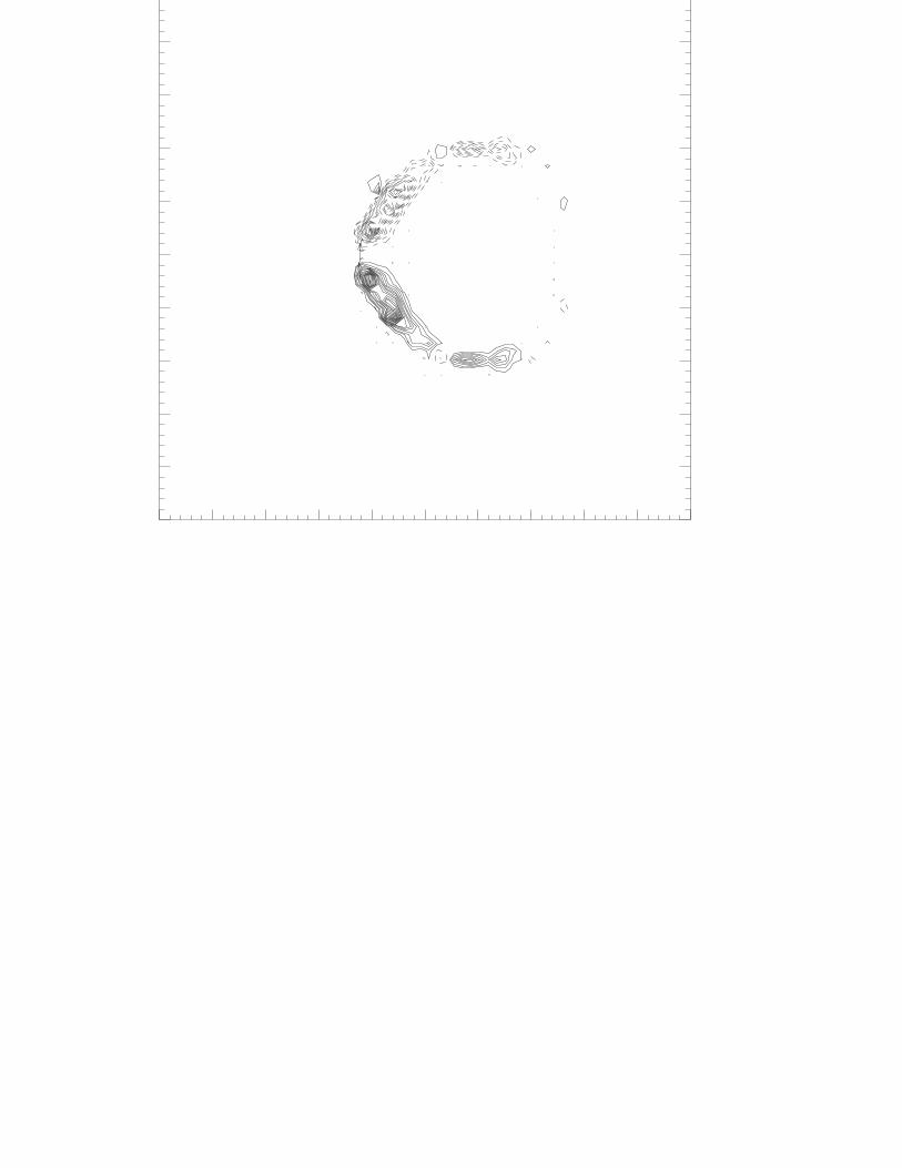
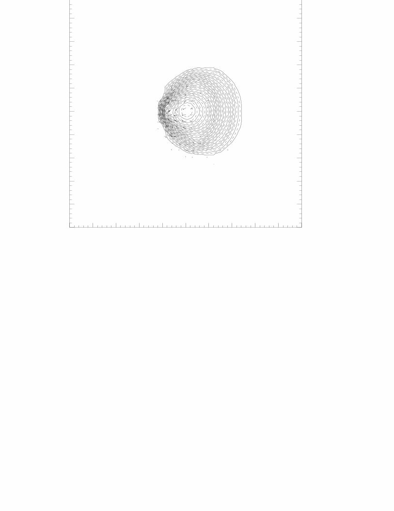
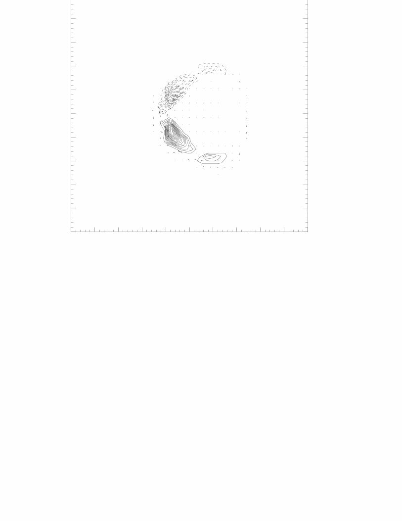
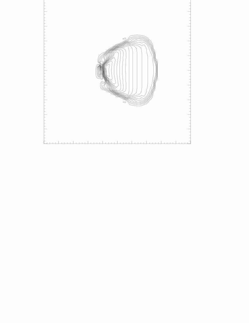
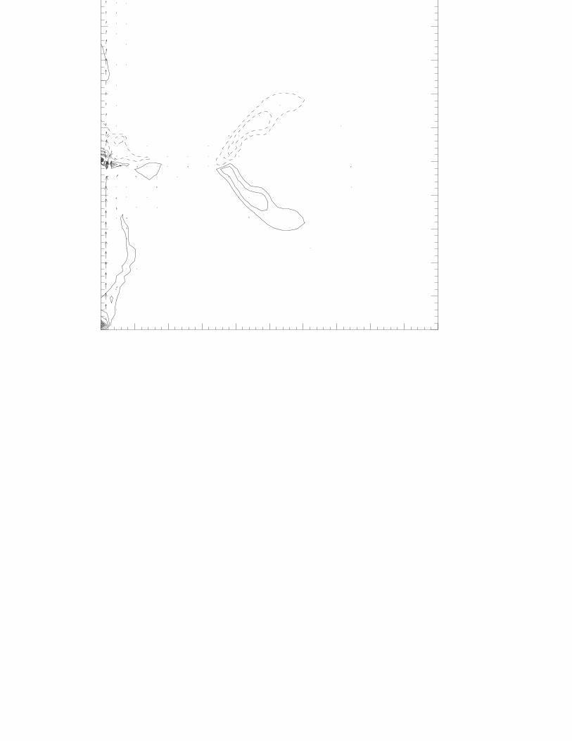
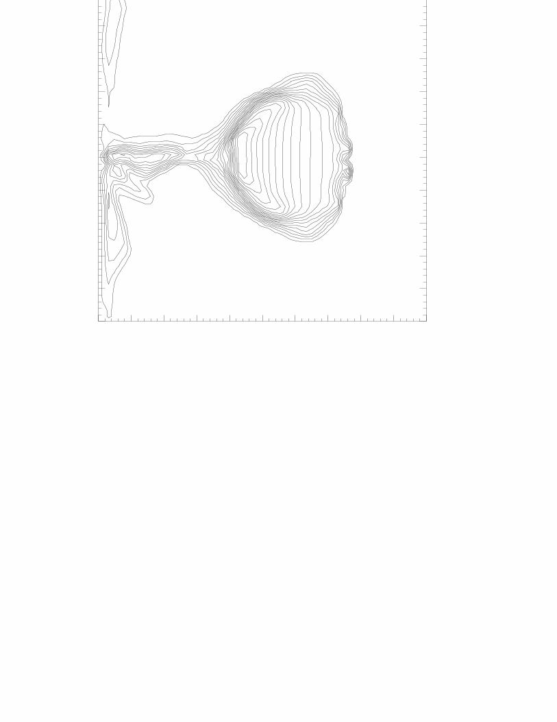
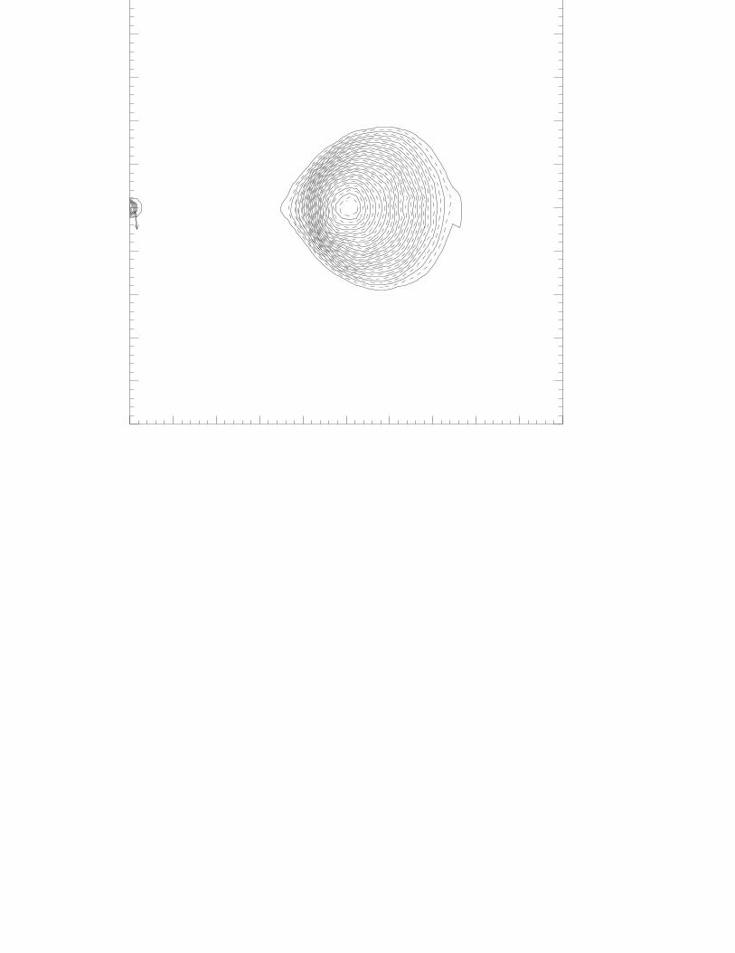
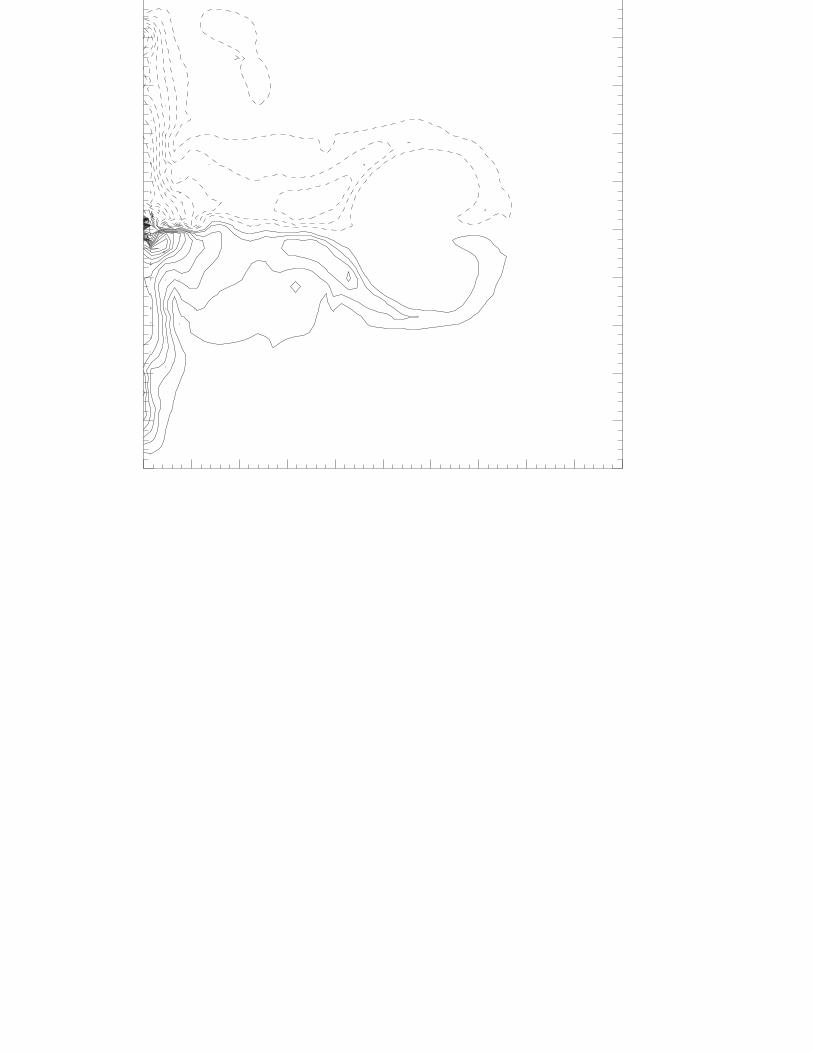
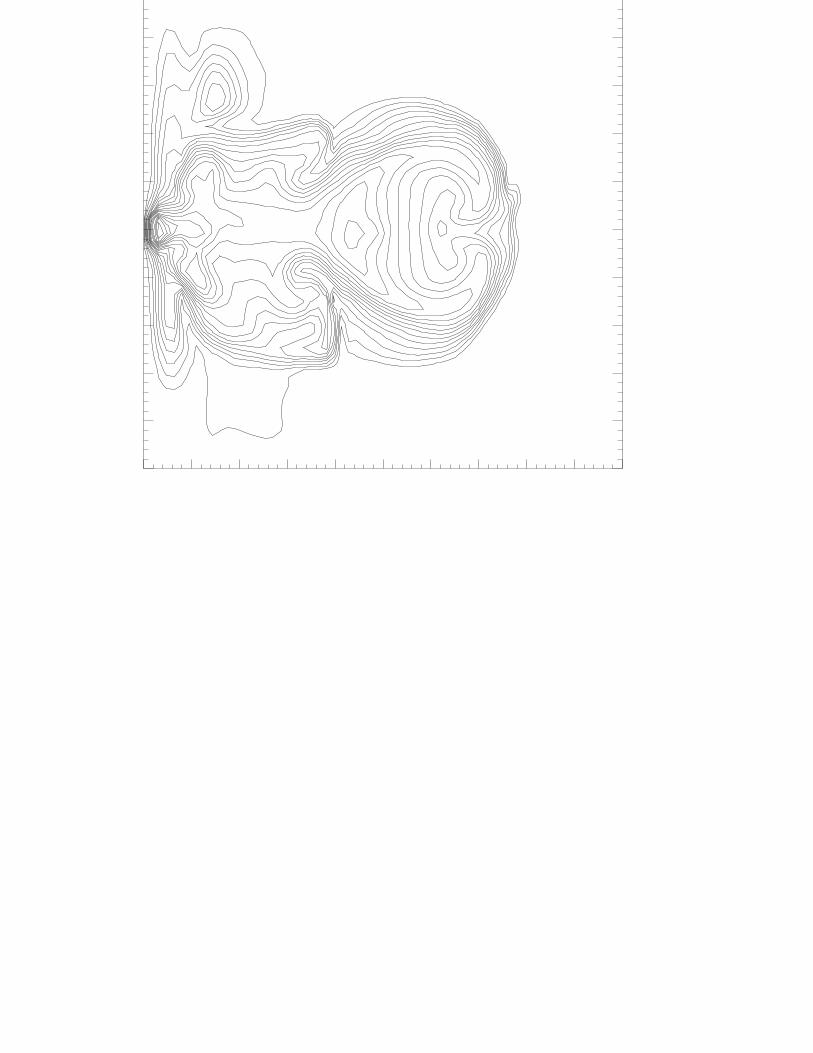
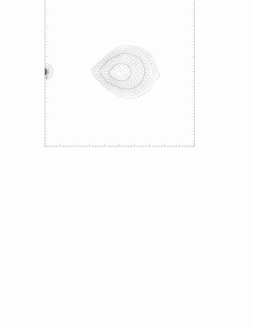
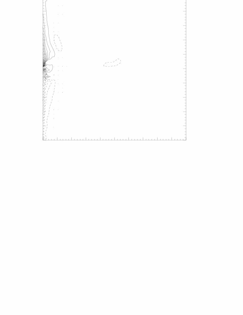
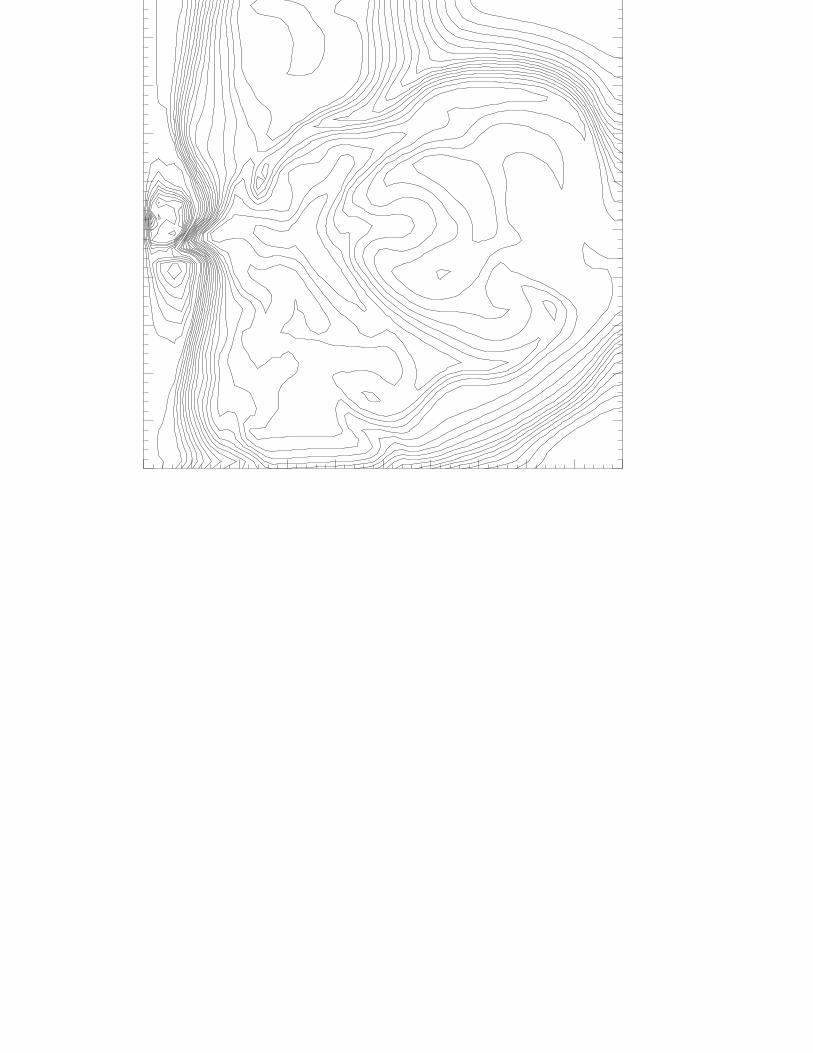
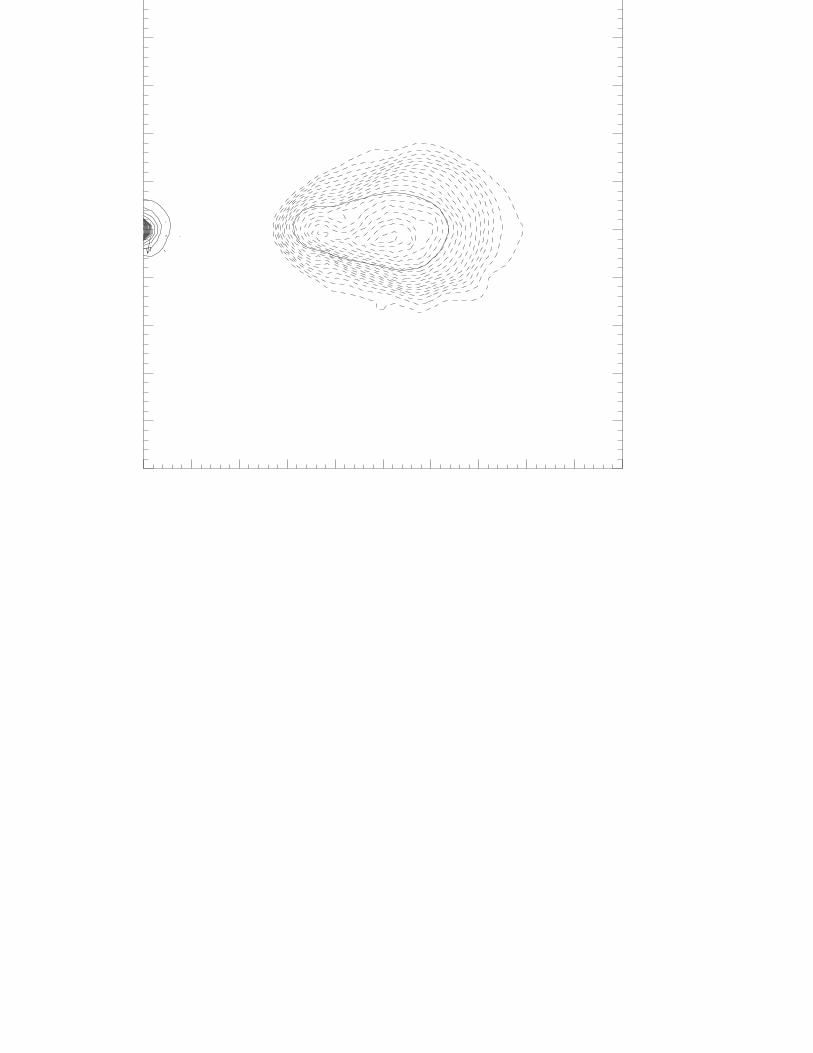
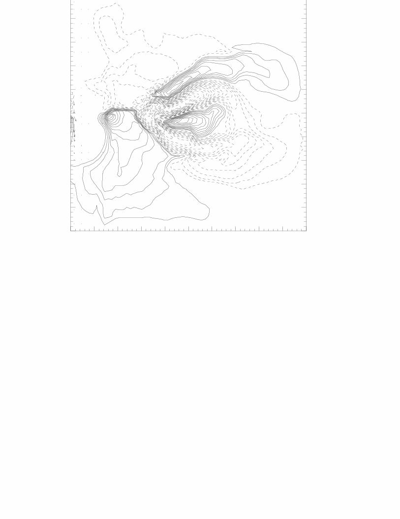
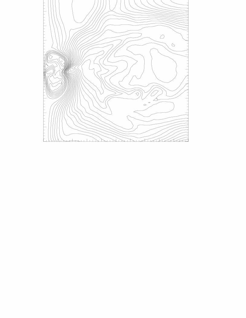
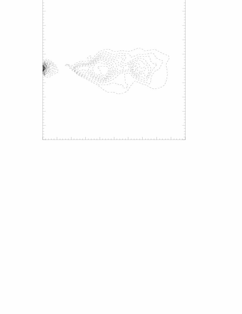
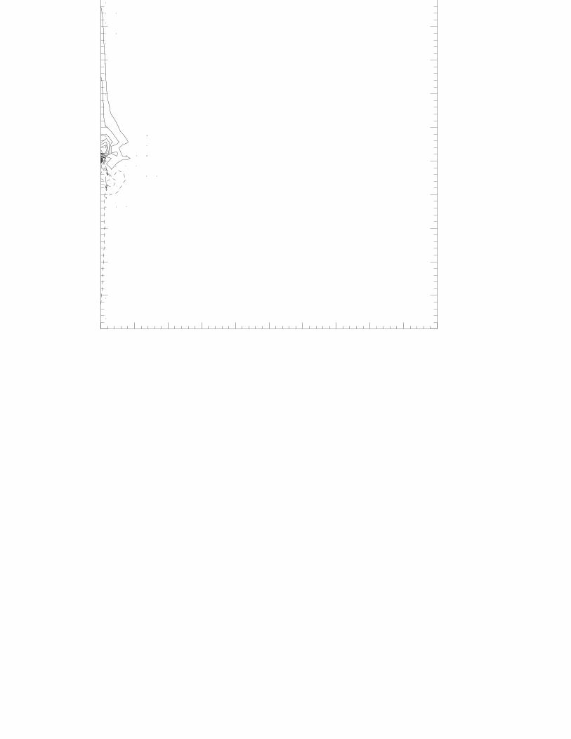
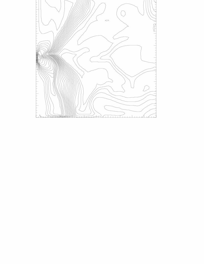
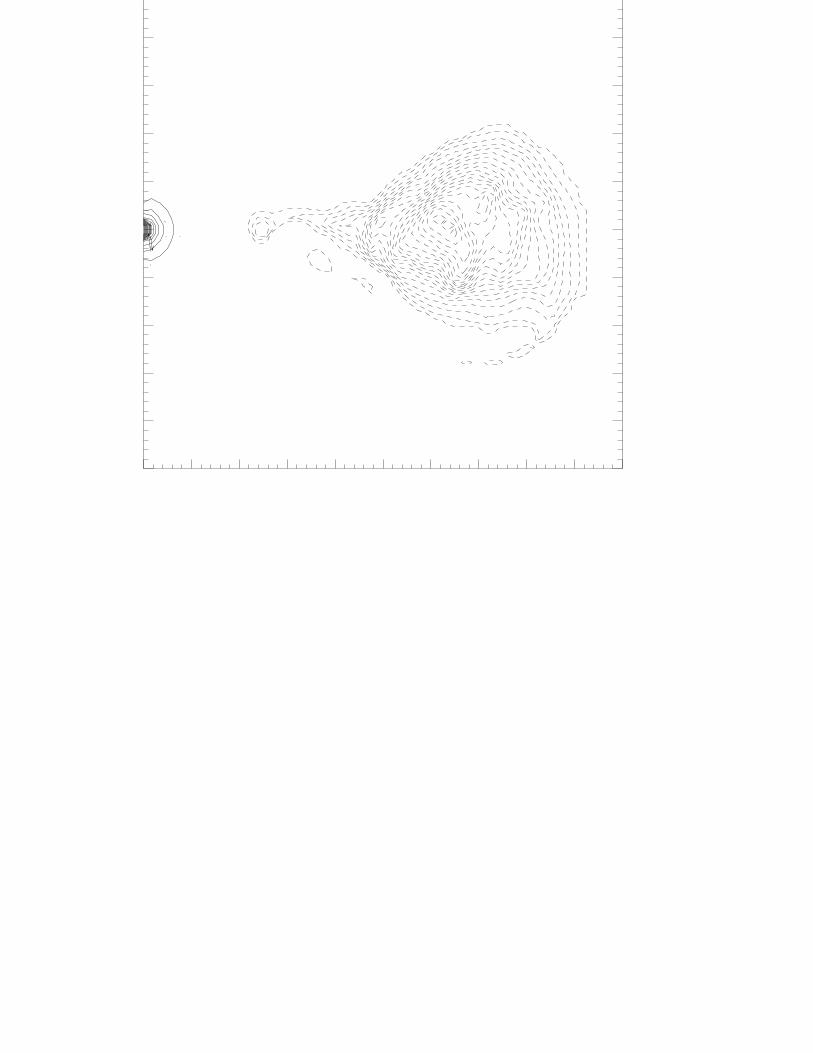
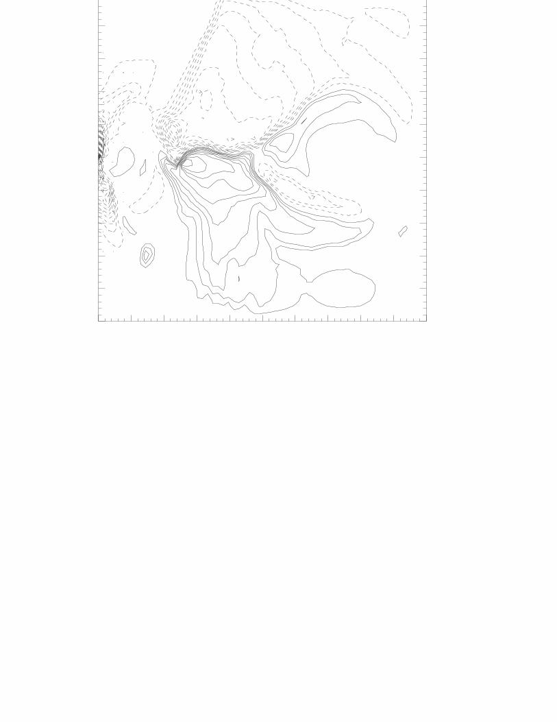
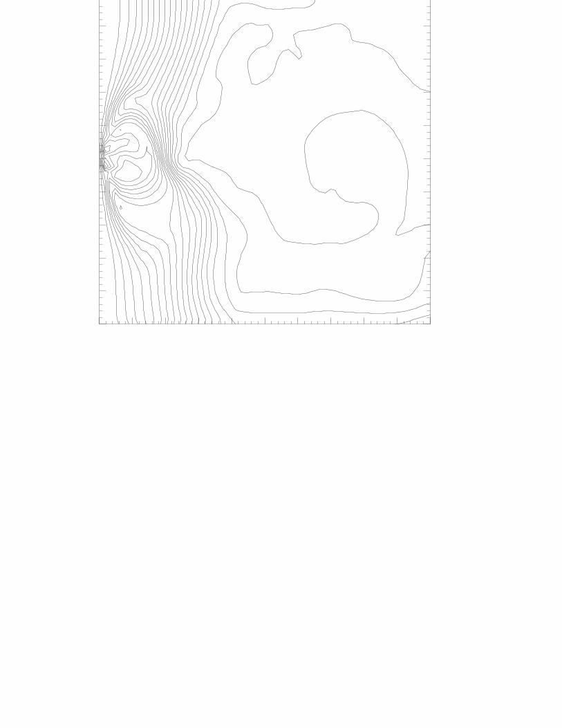
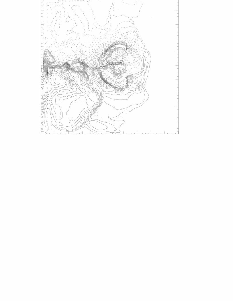
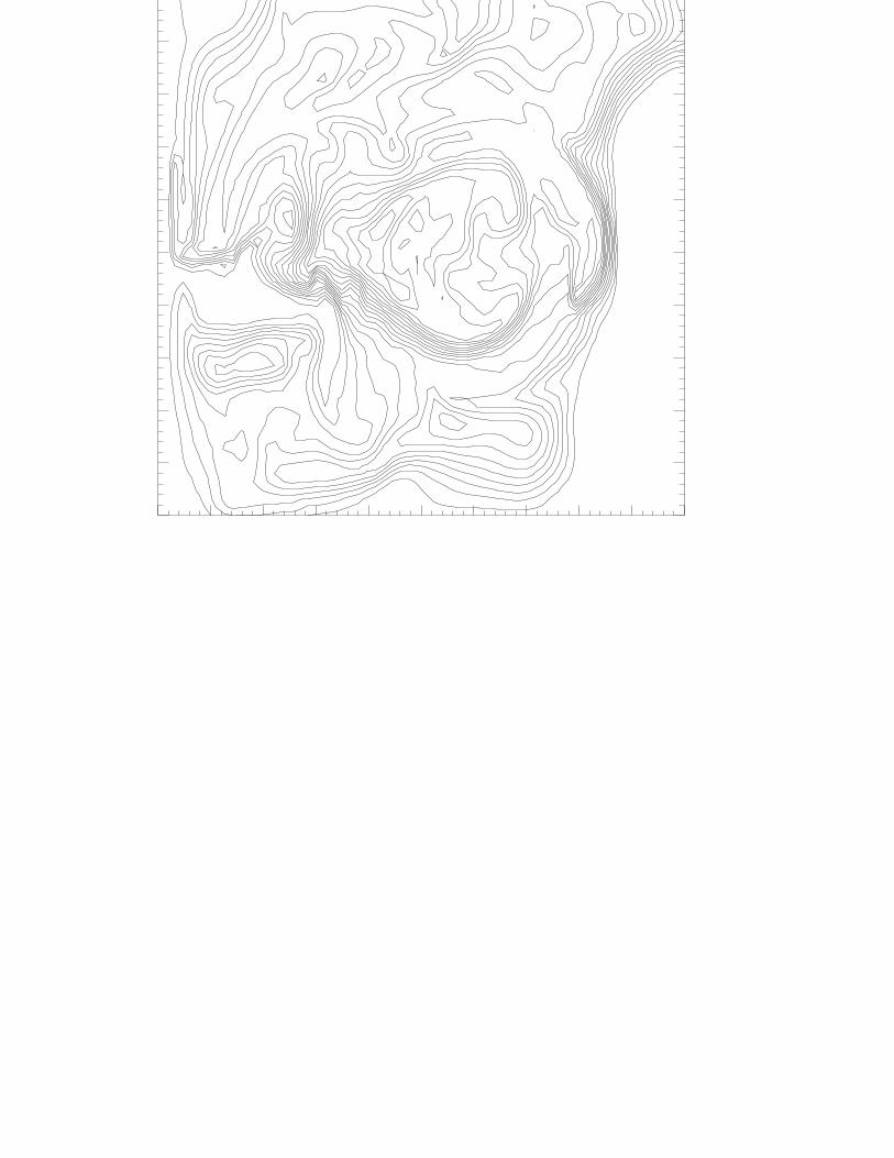
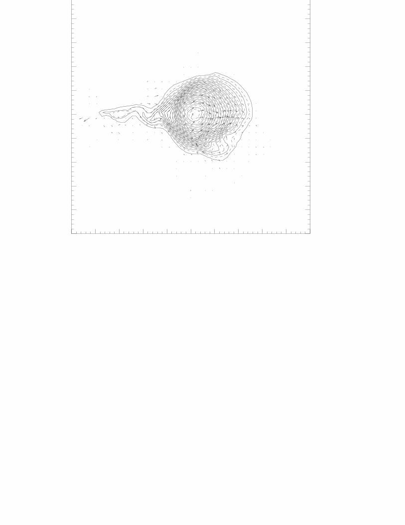
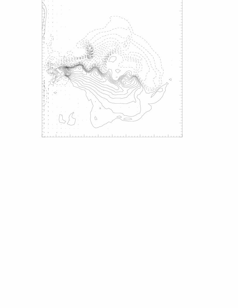
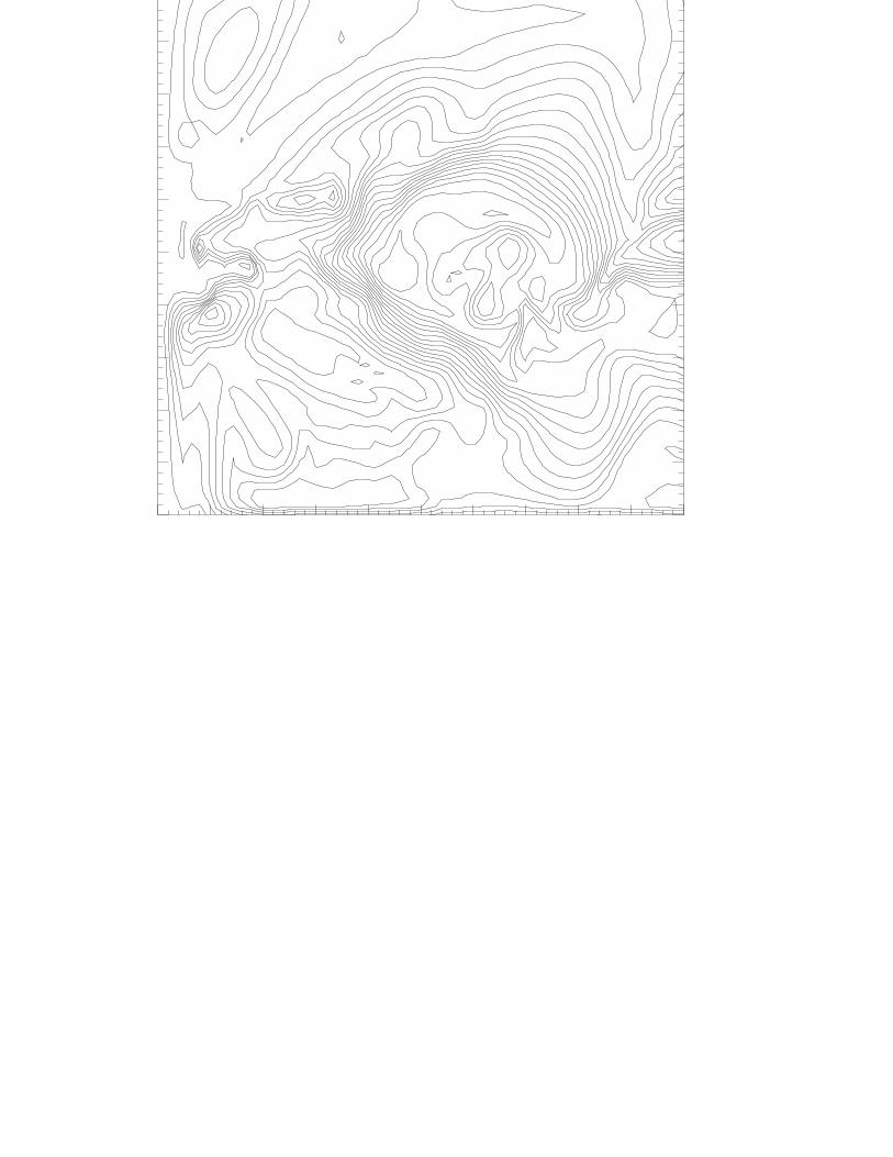
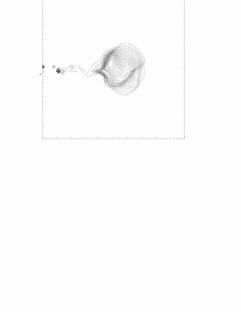
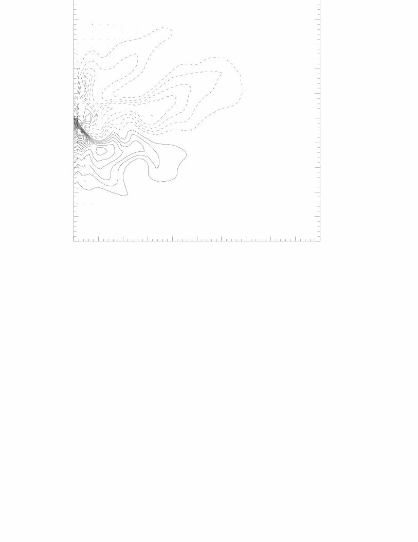
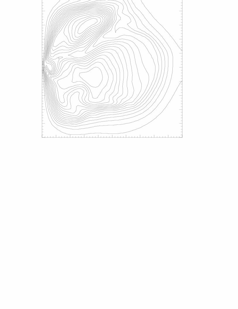
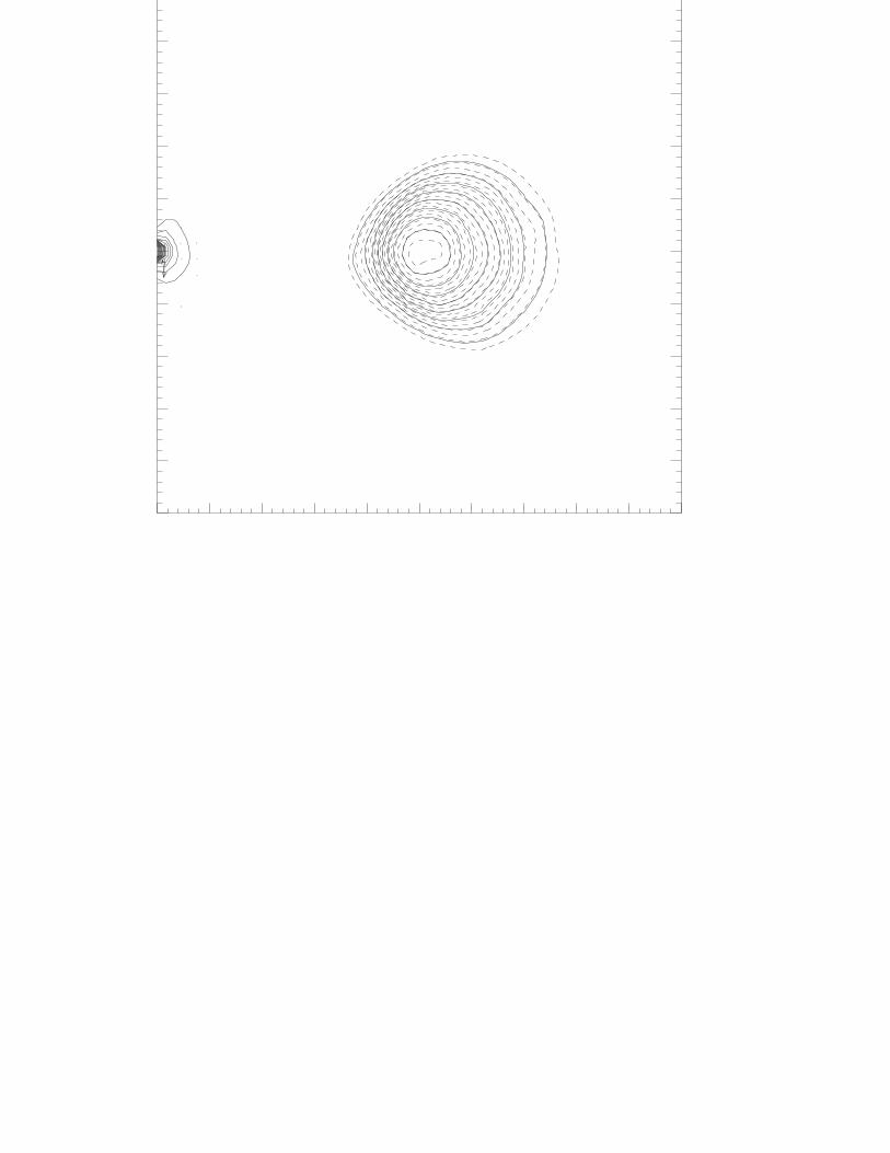
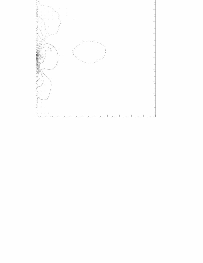
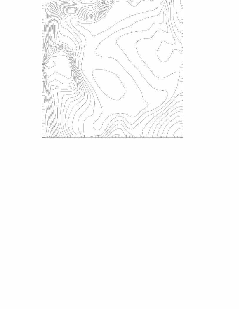
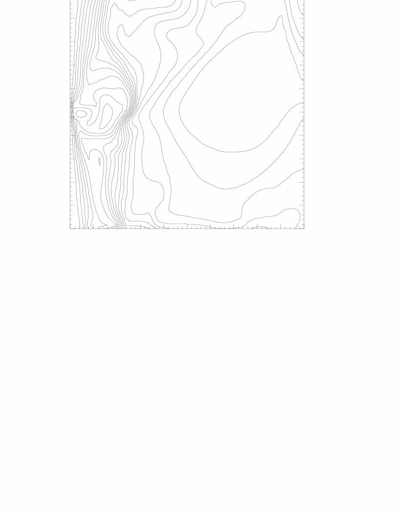
Most of the figures that follow show contour plots and vector fields in the RZ–plane of

each model at various times. These figures have three panels. Panel a shows mass density

contours as solid lines, angular momentum density contours as dashed lines, and poloidal

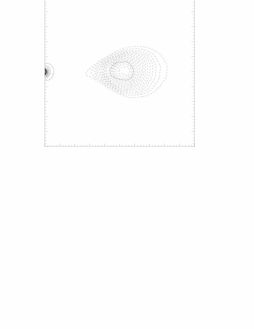
momentum densities as vectors. Panel b shows contours of the toroidal magnetic field (solid

lines in the +φ direction and dashed lines in the −φ direction) and vectors of the poloidal

magnetic field. In each of these two panels, contours are drawn down to the 5% level of the

corresponding maximum value and arrows are drawn down to 10% of the largest magnitude.

In addition, very small vectors with magnitudes between 1% and 10% of the maximum value

are replaced by dots in order to indicate in which regions of the grid the vector fields tend

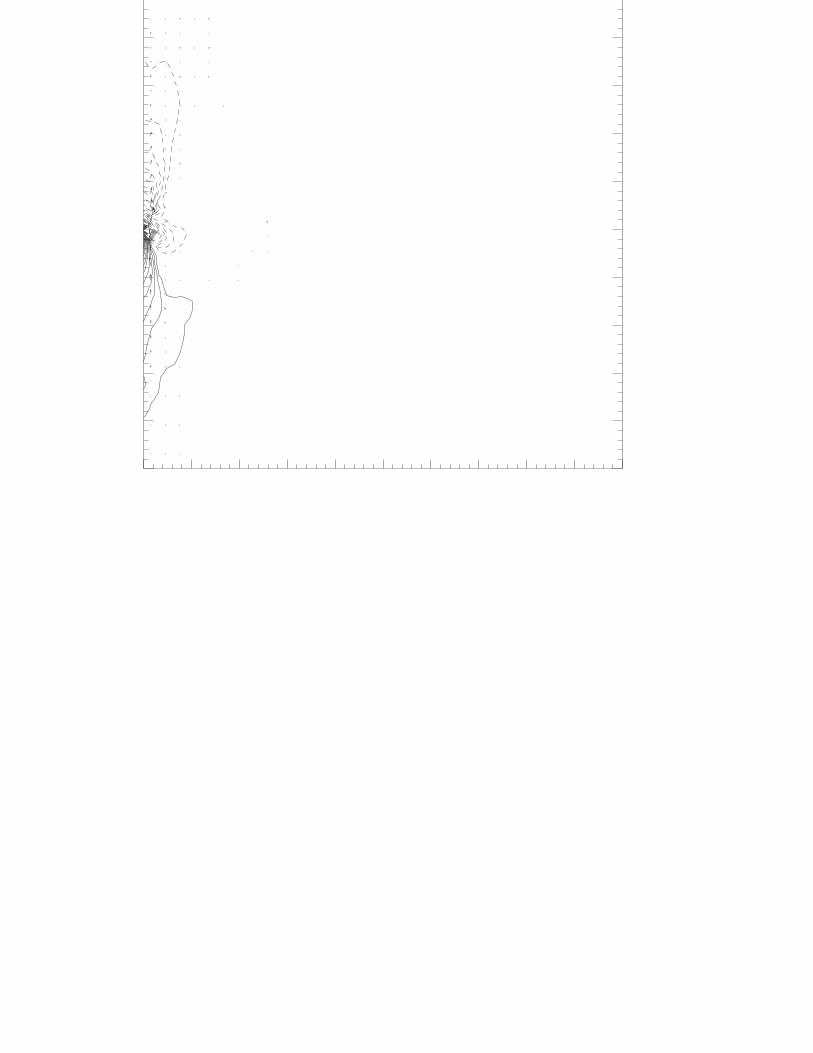
to spread. Finally, panel c shows poloidal–field lines with no regard to field magnitude and

captures the detailed structure of the very weak field as well. The various snapshots were

chosen specifically to exhibit some of the most interesting large–scale features in each model

evolution.

4.1. Standard Model With κ = 0.1

In the beginning of the simulation, poloidal loops of magnetic field are generated in the

torus by the secular PR source term. The field is stronger near the surface of the torus

because the surrounding isothermal atmosphere does not rotate and the gradients of the

angular velocity are largest on the surface (see eq. [20]). The differential rotation of the

fluid twists the poloidal loops quickly and generates a prominent toroidal–field component

around the surface of the fluid (Figs. 2 and 3). The field that is created by this mechanism

is responsible for destabilizing the orbiting fluid through an MRI but the instability does

not take hold immediately because field diffusion works against it, even at this moderate

level of diffusivity. The MRI causes rarefaction waves to propagate radially out within the

fluid (Figs. 2a and 3a). These waves slowly carry outward the angular momentum while

the azimuthal magnetic flux accumulates near the inner edge of the torus, as was predicted

by Christodoulou, Contopoulos, & Kazanas (1996, 2003). After ∼ 2 orbits, the MRI has

managed to destabilize only the inner edge and a little matter enhanced with azimuthal flux

is inflowing toward the central point–mass (Fig. 4). This is also when the first jets are seen to

emanate from the nuclear region. Inside the torus, the instability is suppressed efficiently by

– 15 –

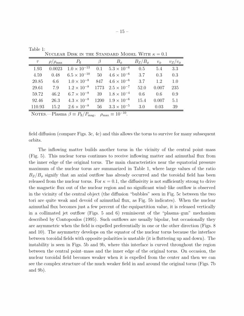
Table 1:Nuclear Disk in the Standard Model With κ = 0.1

τ ρ/ρmax Pfl β Bφ BZ/Bφ vφ vZ/vφ

1.93 0.0023 1.0 × 10−13 0.1 5.3 × 10−6 0.5 5.4 3.3

4.59 0.48 6.5 × 10−10 50 4.6 × 10−6 3.7 0.3 0.3

20.85 6.6 1.0 × 10−8 847 4.6 × 10−6 3.7 1.2 1.0

29.61 7.9 1.2 × 10−8 1773 2.5 × 10−7 52.0 0.007 235

59.72 46.2 6.7 × 10−8 39 1.8 × 10−4 0.6 0.6 0.9

92.46 26.3 4.3 × 10−8 1200 1.9 × 10−6 15.4 0.007 5.1

110.93 15.2 2.6 × 10−8 56 3.3 × 10−5 3.0 0.03 39

Notes.—Plasma β ≡ Pfl/Pmag, ρmax ≡ 10−10.

field diffusion (compare Figs. 3c, 4c) and this allows the torus to survive for many subsequent

orbits.

The inflowing matter builds another torus in the vicinity of the central point–mass

(Fig. 5). This nuclear torus continues to receive inflowing matter and azimuthal flux from

the inner edge of the original torus. The main characteristics near the equatorial pressure

maximum of the nuclear torus are summarized in Table 1, where large values of the ratio

BZ/Bφ signify that an axial outflow has already occurred and the toroidal field has been

released from the nuclear torus. For κ = 0.1, the diffusivity is not sufficiently strong to drive

the magnetic flux out of the nuclear region and no significant wind–like outflow is observed

in the vicinity of the central object (the diffusion “bubbles” seen in Fig. 5c between the two

tori are quite weak and devoid of azimuthal flux, as Fig. 5b indicates). When the nuclear

azimuthal flux becomes just a few percent of the equipartition value, it is released vertically

in a collimated jet outflow (Figs. 5 and 6) reminiscent of the “plasma–gun” mechanism

described by Contopoulos (1995). Such outflows are usually bipolar, but occasionally they

are asymmetric when the field is expelled preferentially in one or the other direction (Figs. 8

and 10). The asymmetry develops on the equator of the nuclear torus because the interface

between toroidal fields with opposite polarities is unstable (it is fluttering up and down). The

instability is seen in Figs. 5b and 9b, where this interface is curved throughout the region

between the central point–mass and the inner edge of the original torus. On occasion, the

nuclear toroidal field becomes weaker when it is expelled from the center and then we can

see the complex structure of the much weaker field in and around the original torus (Figs. 7b

and 9b).

– 16 –

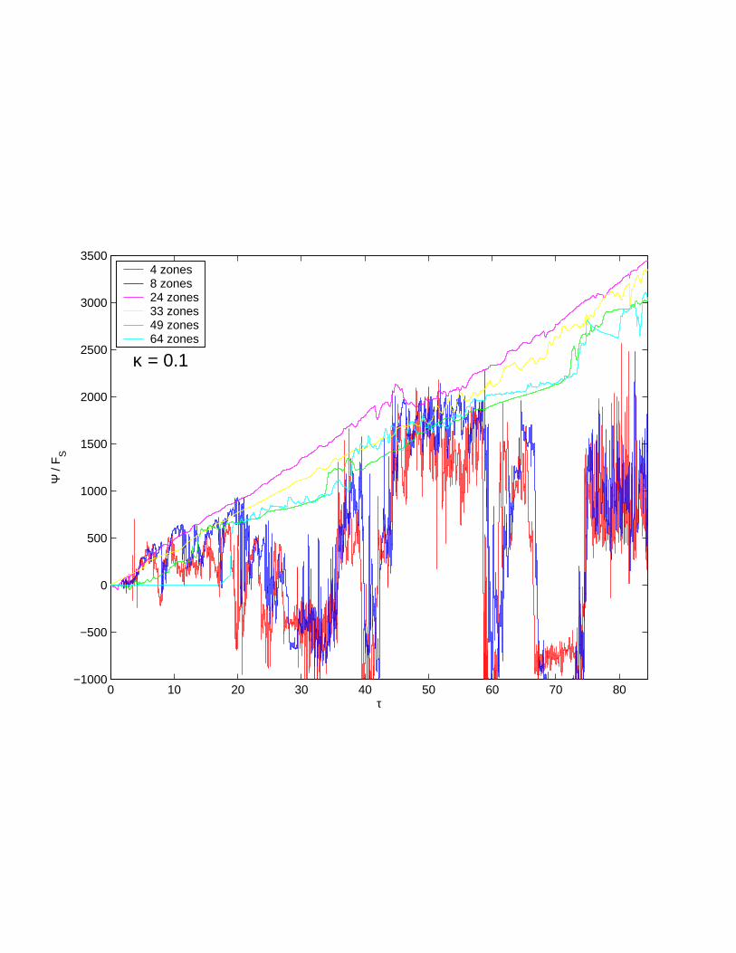
The poloidal magnetic flux

Ψ(R, 0) ≡ 2π

∫ R

0

BZ(R′)R′dR′ , (31)

is monitored over the entire equatorial plane of the computational grid (Fig. 11). Because

the PR source generates complete poloidal loops, the total poloidal flux over the equator of

the grid is zero (loops crossing the equator in one direction have to turn back eventually and

cross in the opposite direction).

The conservation of Ψ(Rmax, 0), where Rmax is the radial edge of the grid, is broken

after 18 orbits when magnetic field from the surface of the torus reaches the outer edge

of the grid and outflows. Then poloidal loops open up at R = Rmax (Figs. 6c, 7c) and

Ψ(Rmax, 0) becomes permanently positive (Fig. 11). In the nuclear torus, the enclosed flux

switches polarity several times and also undergoes high–frequency oscillations due to the

episodic evolution of the nuclear magnetic field (see panels c in Figs. 5–10). At all the other

equatorial radii, and especially in the regions between the two tori and within the original

fluid, the poloidal flux increases linearly with time and this increase continues for more than

80 orbits (Fig. 11), when large amounts of mass and angular momentum reach the radial edge

of the computational grid. Such a steady, gradual increase of the poloidal field was predicted

by CK and CKC for moderate and high levels of diffusivity and owes its linear character to

the time independence of the PR source term S that was included in the induction equation

(eq. [8]).

4.2. Low Resistivity Models With κ ≤ 0.01

In models with κ ≤ 0.01, the diffusion of the field is strong enough to dampen the MRI

and to delay the organized inflow of matter for at least 10 orbits (e.g., Figs. 12a and 13a).

Slow diffusion and the fluttering instability cause the toroidal field to spread away from the

surface of the fluid where it is created. Some of this field is ejected into the surrounding

atmosphere but another part of it diffuses into the fluid of the torus (Fig. 12b). Eventually,

the inner edge of the torus is destabilized by the MRI, loses part of its angular momentum,

and an unbroken stream (a ”sheet”) of inflowing matter is created that is threaded by strong

toroidal magnetic field (Figs. 12b, 14b). In the low resistivity models, a nuclear disk is not

formed. Instead, lumps of matter with embedded field that reach the center ahead of the

inflowing stream are ejected vertically in asymmetric outflows (e.g., Fig. 13a, b).

The entire evolution of these models is reminiscent of the corresponding ideal MHD

model (κ = 0; Fig. 15) except that the ideal MHD fluid is dominated by strong oblique

– 17 –

shocks that distort the torus (Fig. 15a) and that are not observed in models with κ ∼ 0.01

(Fig. 14a). We note that the lump of fluid seen at the center in Fig. 15a will not be the

seed for the formation of a nuclear disk; it will soon be ejected vertically and it will clear

the center for more lumps to come in ahead of the organized inflowing stream that needs

another 6 or 7 orbits to get into the same area.

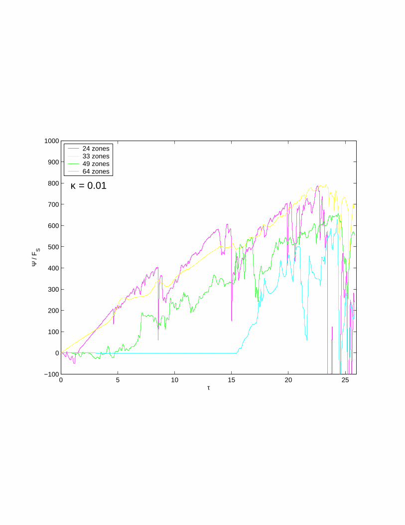
The poloidal magnetic flux at different equatorial radii of the model with κ = 0.01 is

shown in Fig. 16. Although the flux is initially growing linearly with time, this growth is

quickly terminated after about 23 orbits. This is because the toroidal field remains nearly

frozen into the fluid and does not unwind (e.g., Fig. 14b, c). Eventually magnetic reconnec-

tion and the fluttering instability along the equator of the grid limit field growth, while the

new field generated by the PR source is not significant in magnitude to make a difference.

This behavior is intimately linked to the inability of the low–resistivity models to form a

nuclear disk. We have determined by additional simulations that all models with κ ≤ 0.06

present the same characteristics, while two models with κ = 0.065 and κ = 0.07 exhibit

nuclear–disk formation within 3 − 4 orbits and uninterrupted central flux amplification for

20 orbits when these runs were terminated.

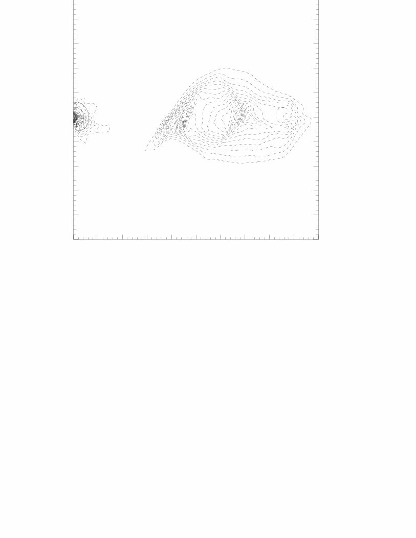
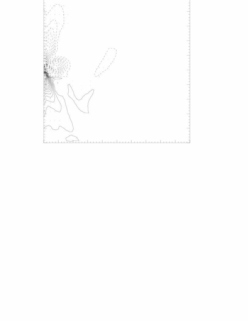
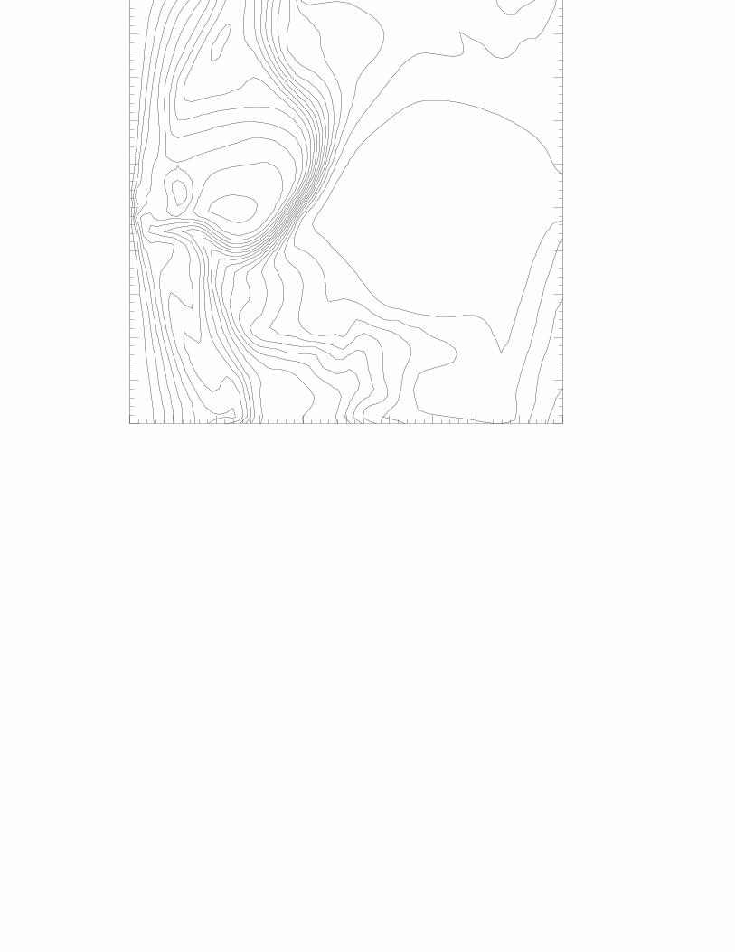
4.3. High Resistivity Models With κ ≥ 1

In models with κ ≥ 1, field diffusion occurs over dynamical timescales and the field

quickly spreads out to the surrounding atmosphere and inward to the fluid of the original

torus. The MRI is damped very efficiently in these simulations and the original torus survives

for more than 140 orbits (Figs. 17–20) when large amounts of outflowing matter and angular

momentum have crossed the outer radial edge of the computational grid. For the first few

orbits, the dominant field is toroidal and it is being built up continually by the differential

rotation of the fluid in the original torus. Most of this field is carried into the nuclear region

where it becomes anchored in the newly formed nuclear torus and diffuses away from it in all

directions (Figs. 17b, 18b and 20b). Inside the original torus, the field is limited efficiently

by magnetic reconnection; it remains very weak, and this is why its does not appear in the

contour plots of the same figures.

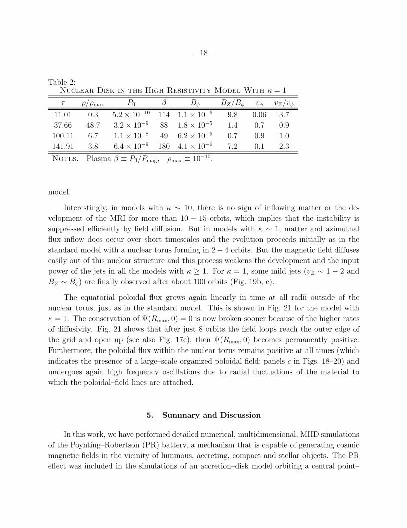
The nuclear torus continues to receive the inflowing matter and azimuthal flux. The

main characteristics near its equatorial pressure maximum are summarized in Table 2. After

the first 30 orbits, this torus ends up rotating faster than the nuclear torus of the standard

model. The fluid is cooler and the axial outflows are weaker and appear much later (at

τ ∼ 100). Magnetic pressure support remains always at a level of at least ∼ 1% of the fluid

pressure, and as a result, the nuclear fluid is always less dense than that of the standard

– 18 –

Table 2:Nuclear Disk in the High Resistivity Model With κ = 1

τ ρ/ρmax Pfl β Bφ BZ/Bφ vφ vZ/vφ

11.01 0.3 5.2 × 10−10 114 1.1 × 10−6 9.8 0.06 3.7

37.66 48.7 3.2 × 10−9 88 1.8 × 10−5 1.4 0.7 0.9

100.11 6.7 1.1 × 10−8 49 6.2 × 10−5 0.7 0.9 1.0

141.91 3.8 6.4 × 10−9 180 4.1 × 10−6 7.2 0.1 2.3

Notes.—Plasma β ≡ Pfl/Pmag, ρmax ≡ 10−10.

model.

Interestingly, in models with κ ∼ 10, there is no sign of inflowing matter or the de-

velopment of the MRI for more than 10 − 15 orbits, which implies that the instability is

suppressed efficiently by field diffusion. But in models with κ ∼ 1, matter and azimuthal

flux inflow does occur over short timescales and the evolution proceeds initially as in the

standard model with a nuclear torus forming in 2− 4 orbits. But the magnetic field diffuses

easily out of this nuclear structure and this process weakens the development and the input

power of the jets in all the models with κ ≥ 1. For κ = 1, some mild jets (vZ ∼ 1 − 2 and

BZ ∼ Bφ) are finally observed after about 100 orbits (Fig. 19b, c).

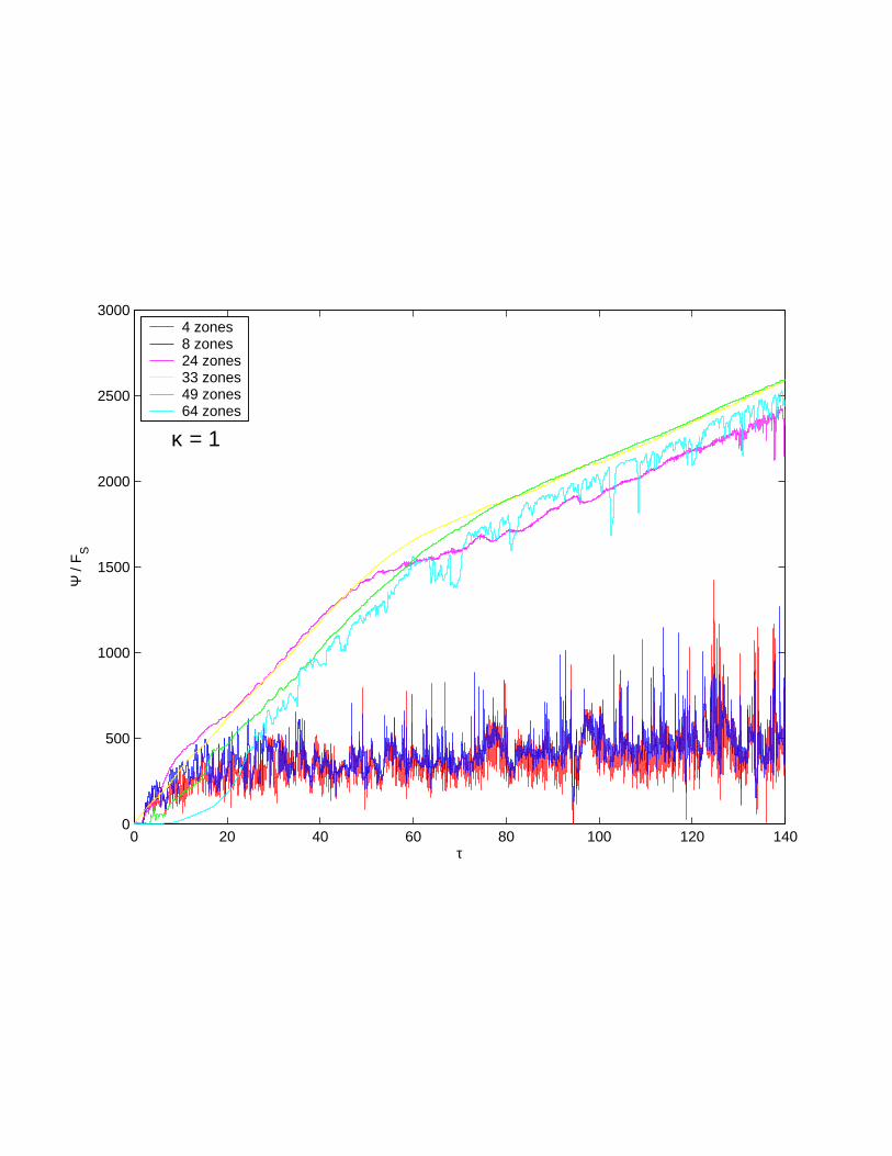
The equatorial poloidal flux grows again linearly in time at all radii outside of the

nuclear torus, just as in the standard model. This is shown in Fig. 21 for the model with

κ = 1. The conservation of Ψ(Rmax, 0) = 0 is now broken sooner because of the higher rates

of diffusivity. Fig. 21 shows that after just 8 orbits the field loops reach the outer edge of

the grid and open up (see also Fig. 17c); then Ψ(Rmax, 0) becomes permanently positive.

Furthermore, the poloidal flux within the nuclear torus remains positive at all times (which

indicates the presence of a large–scale organized poloidal field; panels c in Figs. 18–20) and

undergoes again high–frequency oscillations due to radial fluctuations of the material to

which the poloidal–field lines are attached.

5. Summary and Discussion

In this work, we have performed detailed numerical, multidimensional, MHD simulations

of the Poynting–Robertson (PR) battery, a mechanism that is capable of generating cosmic

magnetic fields in the vicinity of luminous, accreting, compact and stellar objects. The PR

effect was included in the simulations of an accretion–disk model orbiting a central point–

– 19 –

mass by introducing a continuous source of poloidal magnetic field into the induction equation

(eq. [8]). At the same time, the differential rotation of the disk model provided an elemental

source of toroidal magnetic field by twisting dynamically the poloidal field lines. The fluid

in the accretion disk and in a surrounding tenuous nonrotating atmosphere was resistive

and allowed for the magnetic field to diffuse away from the areas where it was originally

produced. In all models, a large–scale accretion flow was established from the initial disk

model toward the central point–mass by the action of a magnetorotational instability (MRI)

in the orbiting fluid. Two of the above features, the PR current that acts as a continuous

source of weak magnetic field and the global accretion flow that may cause its amplification

by drawing field of a single polarity to the center, are what sets the PR battery apart from

previously proposed and critically reviewed mechanisms of field generation and amplification

such as the Biermann (1950) battery and the turbulent dynamo process (see also § 1).

The present simulations constitute a first attempt toward studying the global magne-

tohydrodynamics of resistive large–scale accretion flows and the possible amplification or

saturation of the generated magnetic flux in the presence of various degrees of magnetic

dissipation. The latter is controlled by a free parameter, the resistive frequency κ (eq. [30])

which is a direct measure of the resistivity η of the fluid and inversely proportional to the

electrical conductivity σ. We have found that a value of κ ≈ 0.06 (corresponding to a diffu-

sion timescale τdiff ≈ 16 local dynamical times) is the critical value that separates two types

of physically different model evolutions:

1. Models with moderate and high resistivities (κ > 0.06) exhibit strong field amplifica-

tion that continues uninterrupted for over 100 orbits (Figs. 11 and 21). In about 2− 4

orbits, the inflowing matter creates a nuclear torus near the central point–mass and

the magnetic field that is transported into the nucleus by accretion and by diffusion

becomes anchored onto this torus. When the nuclear toroidal field becomes strong, it

unwinds and produces episodic bipolar jet–like outflows, in addition to the diffusing

field bubbles that are observed to emerge from the center when κ ≥ 1. The equato-

rial field is unstable to fluttering and this instability is responsible for the occasional

appearance of markedly asymmetric vertical jets and for the ejection of magnetic field

into the surrounding atmosphere. All of these details are illustrated in Figs. 2–10 for

our standard model with κ = 0.1 and in Figs. 17–20 for the κ = 1 model.

2. Models with low–resistivities (κ ≤ 0.06) exhibit some moderate field amplification for

about 20 orbits, but then the magnetic field quickly saturates to dynamically insignif-

icant levels because of the weak diffusion and the absence of unwinding of the toroidal

component, as the magnetic field remains nearly frozen into the matter. The accretion

flow carries its magnetic field toward the central point–mass but it does not create a

– 20 –

nuclear torus. Eventually magnetic reconnection, the fluttering instability, and some

asymmetric ejections of magnetized lumps limit the growth of the field to less than 3

orders of magnitude above the values seen early in the model evolutions (Fig. 16). All

of these details are illustrated in Figs. 12–14 for the κ = 0.01 model and in Fig. 15 for

the ideal MHD model with κ = 0.

The above results are in agreement with those discussed by CK and CKC on the basis

of qualitative arguments and more idealized model calculations. The present work provides

further evidence in support of our original conclusions and we are confident that the proposed

battery mechanism will prove important to the theory of generation of cosmic magnetic fields.

The critical value of the inverse magnetic Prandtl number determined by CK, namely

(Pm)−1 ≃ 2, also appears to be in agreement with the critical value of κ ≈ 0.06 determined

from the present simulations, if an allowance is made for a rough, order-of-magnitude es-

timate of the effective viscous timescale τvis associated with turbulent, MRI–driven inflow

from the initial torus under ideal–MHD conditions (when the dynamics is not altered by

resistive slipping of the magnetic field through the matter): In our κ = 0 simulation with

frozen–in magnetic field, the inflowing stream of matter has not reached the center after 19

orbits (Fig. 15) and the continuing evolution shows that this is still the case after 26 orbits

when the stream is getting close to the center. Based on this observation, we estimate that

τvis ≈ 26τdyn, where τdyn is the local dynamical time in the initial torus. Since the critical

κ ≈ 0.06 implies that τdiff ≈ 16τdyn, then the critical inverse magnetic Prandtl number in

the resistive simulations is

(Pm)−1 =τvis

τdiff

≃ 1.6 , (32)

and field amplification occurs for κ > 0.06 or, equivalently, for (Pm)−1 > 1.6. We note that

the above value of τvis implies also an effective value of αmag>∼ 0.04 for the analogue of the

Shakura–Sunyaev (1973) parameter of the accretion flow initiated by the MRI in the ideal–

MHD model. This is just a rough estimate and as such it is not out of line compared to values

determined previously from simulations of the MRI in the ideal–MHD limit (αmag ∼ 0.1;

Hawley & Krolik [2002] and references therein). But notice that the effective αmag–parameter

increases dramatically to a value of αmag ≈ 0.3−0.5 in the κ > 0.06 models in which a robust

nuclear disk forms in just a few orbits. We have to conclude then that a sufficient amount

of magnetic diffusivity appears to be the cause of dynamical nuclear–disk formation in the

above resistive models.2

2This conclusion should not be confused with the conclusions of Stone & Pringle (2001) and Hawley &

Balbus (2002) who see the fluttering instability and the formation of the nuclear disk but find no purely axial,

collimated outflow and no substantial differences in their models when a small amount of artificial resistivity

– 21 –

All the simulations of models with κ > 0 show that field diffusion works against the

MRI and this instability is damped with increasing success as the value of κ is increased.

This result is known and well–understood (e.g., Fleming, Stone, & Hawley 2000; Fleming

& Stone 2003). When the magnetic field is allowed to slip through the matter, then the

field lines cannot hold on to specific fluid elements and facilitate their exchange of angular

momentum and azimuthal magnetic flux. However, the MRI is not eliminated from any

model with a reasonable value of κ and the weakened modes continue to transport some

of the angular momentum to larger radii and matter with enhanced azimuthal magnetic

flux toward the central point–mass (see also Christodoulou, Contopoulos, & Kazanas 1996,

2003). In the moderate and high–resistivity models (κ ≥ 0.1), the transfer of these conserved

quantities is gradual and this allows the original accretion tori to survive for hundreds of

orbits (in our simulations, it takes 80 − 140 orbits for substantial amounts of matter and

angular momentum to cross the outer radial edge of the grid, a distance only twice as large

as the characteristic size of the initial torus).

In our model evolutions, we strengthened artificially the PR source because the current

state of computing does not allow us to run MHD models with a weak PR source and wait

for millions of dynamical times to see whether the magnetic field will be amplified or not

(§ 2.2). Even with an artificially enhanced PR source, however, the initial magnetic field is

1 − 2 orders of magnitude smaller than that utilized to induce an MRI in previous MHD

simulations (e.g. Hawley 2000; Hawley, Balbus, & Stone 2001): At early times (τ >∼ 0.1), the

poloidal field grows at the inner edge of the initial torus to ∼ 10−9, a value that results in a

plasma β ∼ 5 × 104. Within the first orbit, the toroidal field also catches up in magnitude

and at later times, all field components are amplified as the magnetic field is drawn into the

nuclear region. The amplification of the poloidal flux is eventually interrupted (at τ ∼ 20) in

the low–resistivity models, as discussed above and in § 4.2. The amplification of the toroidal

flux in the κ > 0.06 models is also interrupted episodically by the repeated unwinding of the

toroidal field that accumulates in the nuclear torus. This effect is a version of the “plasma–

is included to smear out current sheets. These simulations were essentially carried out using ideal MHD;

as such, they can see the intrinsic instability of the equatorial toroidal field and the large–scale structure

of the accreted fluid, but they cannot capture the influence of moderate or large amounts of anomalous

resistivity. Furthermore, the inflowing stream in these ideal–MHD simulations reaches the center in just 2

orbits. Such inflow is too fast, essentially dynamical, and it does not appear in line with the values of the

effective αmag–parameter (∼ 0.05− 0.1) reported for the fluid in the original torus when it is destabilized by

the MRI. Stone & Pringle (2001) claim that global stresses of the radial magnetic field are responsible for

this early outward transport of angular momentum and the associated inflow that occurs before the MRI

actually becomes nonlinear. But no such global stresses are observed in our κ = 0 simulation in which the

magnetosonic rarefaction waves take time to transverse the fluid, to redistribute the conserved quantities

locally, and finally to drive the MRI into the nonlinear regime.

– 22 –

gun” expulsion suggested by Contopoulos (1995): when the toroidal field grows close to

equipartition in the nuclear torus, it can no longer be confined; it is released dynamically

in the vertical direction and its stresses act to confine the poloidal–field component close to

the symmetry axis of the torus. This situation is evident in many of the diagrams (panels

c) shown in § 4.1 and § 4.3, where the poloidal field lines are nearly vertical at small radii

and the “funnels” along the Z–axis are extremely narrow. At the same time, the b–panels

of the same figures depict the substantial degree of collimation imposed by the toroidal field

to the low–density matter flowing within these funnels. These results are of interest because

they demonstrate that the anomalous resistivity in the accretion flows and the plasma–gun

mechanism may be responsible for producing the highly collimated jets observed in a variety

of accretion–powered galactic and extragalactic objects (see, e.g., Bridle & Perley 1984;

Mirabel & Rodrıguez 1999; and Wilson, Young, & Shopbell 2001).

Furthermore, our results indicate that the magnetic diffusivity plays a more important

role in accretion disks than previously thought. For moderate or large values of this pa-

rameter (or, equivalently, for values of the resistive frequency κ > 0.06), there is a clear

tendency in the models to generate and maintain strong, well–ordered, large–scale poloidal

magnetic fields which couple to the rotation of the nuclear flow and result in matter expulsion

along the rotation axis. In contrast, no such features are seen at large scales in models with

κ ≤ 0.06. Therefore, our models suggest that the well–known and well–defined dichotomy of

accretion–powered objects (e.g., Xu, Livio, & Baum 1999; Ivezic et al. 2004) to those ex-

hibiting powerful jets (“radio–loud”) and those lacking such structures (“radio–quiet”) may

be related to and should be sought in the physics that determines the value of this particular

macroscopic parameter of the accretion flows that power the emission of these objects. The

calculations presented here are only a preliminary step toward exploring this notion.

This work was supported in part by a Chandra grant.

REFERENCES

Balbus, S. A., & Hawley, J. F. 1991, ApJ, 376, 214

Balbus, S. A., & Hawley, J. F. 1998, Rev. Mod. Phys., 70, 1

Biermann, L. 1950, Z. Naturforsch, 5a, 65

Bisnovatyi-Kogan, G. S., & Blinnikov, S. I. 1977, a, 59, 111

Bisnovatyi-Kogan, G. S., Lovelace, R. V. E., & Belinski, V. A. 2002, ApJ, 580, 380

– 23 –

Bridle, A. H., & Perley, R. A. 1984, ARA&A, 22, 319

Christodoulou, D. M., Cazes, J. E., & Tohline, J. E. 1997, New Astronomy, 2, 1

Christodoulou, D. M., Contopoulos, J., & Kazanas, D. 1996, ApJ, 462, 865

Christodoulou, D. M., Contopoulos, J., & Kazanas, D. 2003, ApJ, 586, 372

Christodoulou, D. M., & Sarazin, C. L. 1996, ApJ, 463, 80

Contopoulos, J. 1995, ApJ, 450, 616

Contopoulos, I., & Kazanas, D. 1998, ApJ, 508, 859 (CK)

Contopoulos, I., Kazanas, D., & Christodoulou, D. M. 2006, ApJ, 652, 1451 (CKC)

Evans, C. R., & Hawley, J. F. 1988, ApJ, 332, 659

Fleming, T. P., & Stone, J. M. 2003, ApJ, 585, 908

Fleming, T. P., Stone, J. M., & Hawley, J. F. 2000, ApJ, 530, 464

Hawley, J. F. 2000, ApJ, 528, 462

Hawley, J. F., & Balbus, S. A. 2002, ApJ, 573, 738

Hawley, J. F., Balbus, S. A., & Stone, J. M. 2001, ApJ, 554, L49

Hawley, J. F., & Krolik, J. H. 2002, ApJ, 566, 164

Igumenshchev, I. V., Narayan, R., & Abramowicz, M. A. 2003, ApJ, 592, 1042

Ivezic, Z., Richards, G. T., Hall, P. B., Lupton, R. H., Jagoda, A. S., Knapp, G. R., Gunn,

J. E., Strauss, M. A., Schlegel, D., Steinhardt, W., & Siverd, R. J. 2004, ASP Conf.

Ser., 311, 347

Kulsrud, R. M., Cen, R., Ostriker, J. P., & Ryu, D. 1997, ApJ, 480, 481

Mirabel, I. F., & Rodrıguez, L. F. 1999, ARA&A, 37, 409

Narayan, R., & Yi, I. 1994, ApJ, 428, L13

Papaloizou, J. C. B., & Pringle, J. E. 1984, MNRAS, 208, 721

Shakura, N. I., & Sunyaev, R. A. 1973, A&A, 24, 337

Stone, J. M., Hawley, J. F., Evans, C. R., & Norman, M. L. 1992, ApJ, 388, 415

– 24 –

Stone, J. M., & Norman, M. L. 1992a, ApJS, 80, 753

Stone, J. M., & Norman, M. L. 1992b, ApJS, 80, 791

Stone, J. M., & Pringle, J. E. 2001, MNRAS, 322, 461

Tohline, J. E. 1988, unpublished

Vainshtein, S. I., & Rosner, R. 1991, ApJ, 376, 199

van Leer, B. 1977, J. Comp. Phys., 23, 276

van Leer, B. 1979, J. Comp. Phys., 32, 101

Wilson, A. S., Young, A. J., & Shopbell, P. L. 2001, ApJ, 547, 740

Xu, C., Livio, M., & Baum, S. 1999, AJ, 118, 1169

This preprint was prepared with the AAS LATEX macros v5.2.

– 25 –

FIGURE CAPTIONS

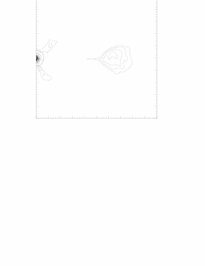
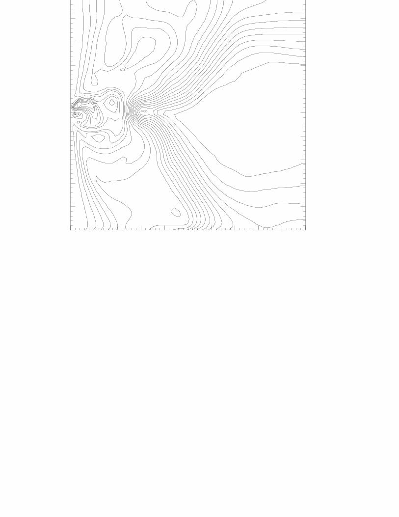
Fig. 1.— Flowchart for the completion of one timestep in the MHD code.

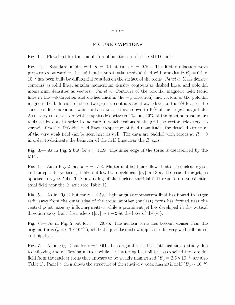
Fig. 2.— Standard model with κ = 0.1 at time τ = 0.76. The first rarefaction wave

propagates outward in the fluid and a substantial toroidal field with amplitude Bφ = 6.1 ×10−7 has been built by differential rotation on the surface of the torus. Panel a: Mass density

contours as solid lines, angular momentum density contours as dashed lines, and poloidal

momentum densities as vectors. Panel b: Contours of the toroidal magnetic field (solid

lines in the +φ direction and dashed lines in the −φ direction) and vectors of the poloidal

magnetic field. In each of these two panels, contours are drawn down to the 5% level of the

corresponding maximum value and arrows are drawn down to 10% of the largest magnitude.

Also, very small vectors with magnitudes between 1% and 10% of the maximum value are

replaced by dots in order to indicate in which regions of the grid the vector fields tend to

spread. Panel c: Poloidal–field lines irrespective of field magnitude; the detailed structure

of the very weak field can be seen here as well. The data are padded with zeroes at R = 0

in order to delineate the behavior of the field lines near the Z–axis.

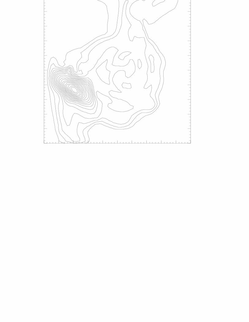
Fig. 3.— As in Fig. 2 but for τ = 1.19. The inner edge of the torus is destabilized by the

MRI.

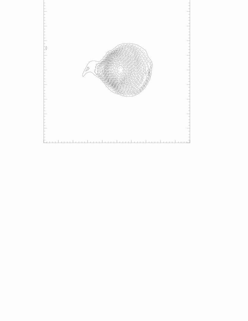
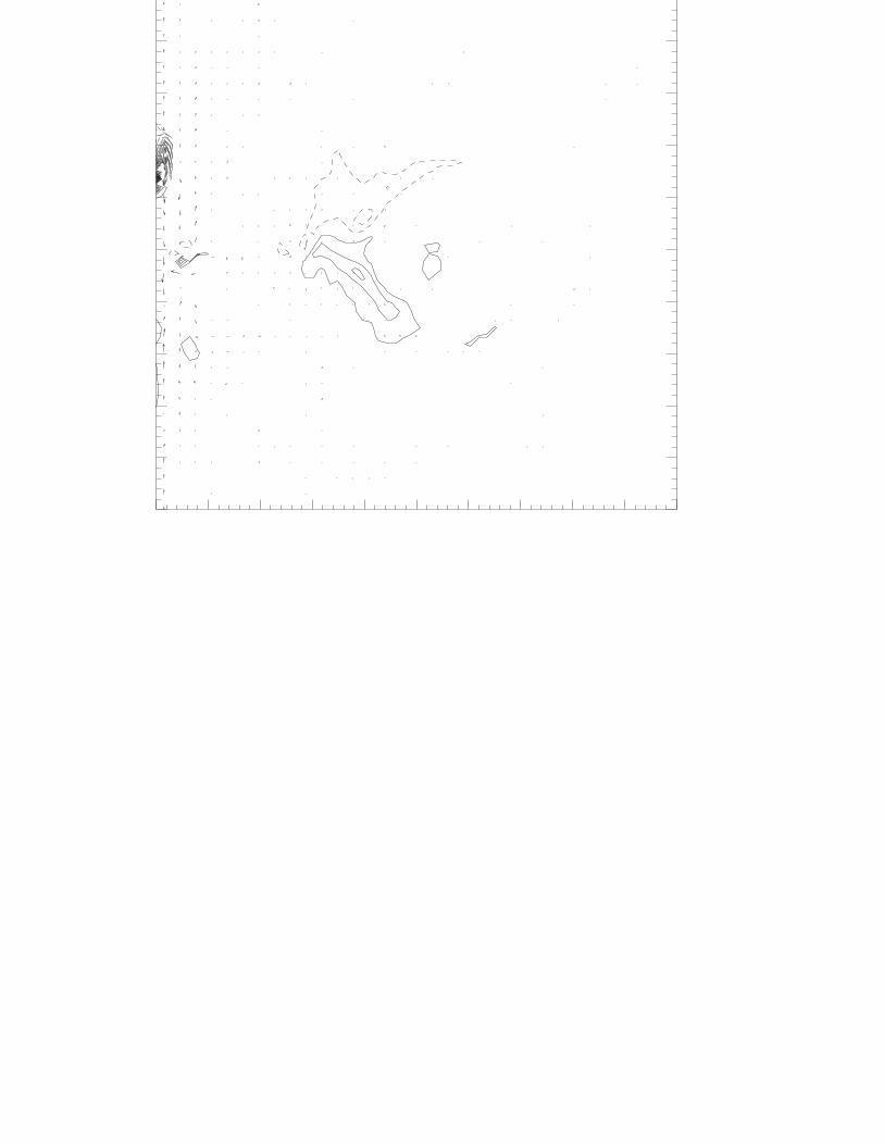
Fig. 4.— As in Fig. 2 but for τ = 1.93. Matter and field have flowed into the nuclear region

and an episodic vertical jet–like outflow has developed (|vZ| ≈ 18 at the base of the jet, as

opposed to vφ ≈ 5.4). The unwinding of the nuclear toroidal field results in a substantial

axial field near the Z–axis (see Table 1).

Fig. 5.— As in Fig. 2 but for τ = 4.59. High–angular momentum fluid has flowed to larger

radii away from the outer edge of the torus, another (nuclear) torus has formed near the

central point mass by inflowing matter, while a prominent jet has developed in the vertical

direction away from the nucleus (|vZ | ∼ 1 − 2 at the base of the jet).

Fig. 6.— As in Fig. 2 but for τ = 20.85. The nuclear torus has become denser than the

original torus (ρ = 6.6×10−10), while the jet–like outflow appears to be very well collimated

and bipolar.

Fig. 7.— As in Fig. 2 but for τ = 29.61. The original torus has flattened substantially due

to inflowing and outflowing matter, while the fluttering instability has expelled the toroidal

field from the nuclear torus that appears to be weakly magnetized (Bφ = 2.5×10−7; see also

Table 1). Panel b then shows the structure of the relatively weak magnetic field (Bφ ∼ 10−6)

– 26 –

that has spread into the original torus and in the surrounding atmosphere.

Fig. 8.— As in Fig. 2 but for τ = 59.72. The original torus has separated into two regions

and the outer region is moving outward. The nuclear torus has become very dense, hot, and

strongly magnetized (Table 1). This torus appears to also support an asymmetric jet–like

outflow with a strong magnetic field (Pmag ∼ Pfl) embedded into the diffuse (ρ ∼ 10−12)

outflowing matter.

Fig. 9.— As in Fig. 2 but for τ = 92.46. The original torus continues to feed matter to the

nuclear region and to move radially outward, while another vertical outflow (|vZ | ∼ 2 at its

base) is taking place in the nuclear torus.

Fig. 10.— As in Fig. 2 but for τ = 110.93. The nuclear disk has expelled much of its own

angular momentum in a wind and it has also developed another asymmetric vertical outflow.

Only 9.7% of the initial mass and 2.0% of the initial angular momentum remain within the

computational grid at this time.

Fig. 11.— Poloidal magnetic flux Ψ(R, 0) on the equatorial plane of the grid, integrated

out to different radii, for the standard model with κ = 0.1. The integrated flux beyond the

nuclear torus increases linearly with time for over 80 orbits, while the flux within the nuclear

torus oscillates at very high frequencies and switches polarity several times.

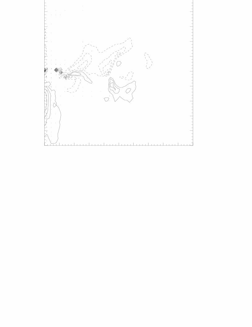
Fig. 12.— Low resistivity model with κ = 0.01 at time τ = 7.50. Two rarefaction waves carry

angular momentum outward in the torus, a ”sheet” of inflowing matter has developed toward

the nucleus, and the fluttering instability has pushed field into the surrounding atmosphere.

The toroidal field presents quite a complex distribution, but it is weak in magnitude (∼ 10−7

or smaller).

Fig. 13.— As in Fig. 12 but for τ = 10.38. Matter in the nuclear region does not get

organized in a disk; instead it is ejected asymmetrically in the vertical direction (vZ ≈ 5)

along with its embedded toroidal field (Bφ ∼ 10−6), while a weak axial–field component

(BZ ∼ 10−7) also develops at small radii.

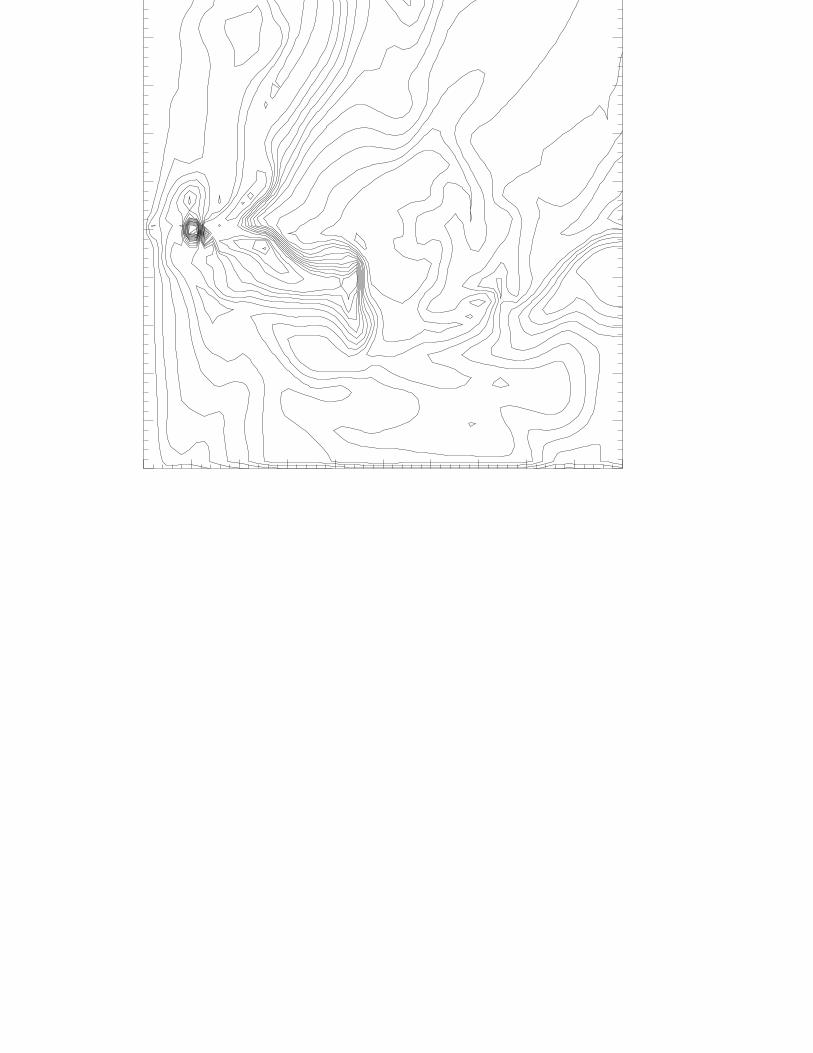
Fig. 14.— As in Fig. 12 but for τ = 16.30. No nuclear disk has developed and the asymmetric

vertical outflow continues in the inner region, while the inflowing sheet of material appears

to be threaded by strong magnetic field (all components are ∼ 10−6). Only 3.5% of the

initial mass and 3.7% of the initial angular momentum has flowed out of the computational

grid at this time.

Fig. 15.— Ideal MHD model with κ = 0 at time τ = 18.86. No field diffusion occurs in

this model and the field remains permanently frozen into the fluid. This model evolution

– 27 –

is similar to the low resistivity model shown in Fig. 14 above, except for the strong oblique

shocks observed here within the fluid of the original torus and at the tip of the inflowing

sheet. Only 3.1% of the initial mass and 3.2% of the initial angular momentum has flowed

out of the computational grid at this time.

Fig. 16.— Poloidal magnetic flux Ψ(R, 0) on the equatorial plane of the grid, integrated out

to different radii, for the low resistivity model with κ = 0.01. The integrated flux no longer

increases linearly with time at times τ > 23.

Fig. 17.— High resistivity model with κ = 1 at time τ = 11.01. A nuclear torus has formed

from inflow and a strong magnetic field (BZ ∼ 10−5, Bφ ∼ 10−6) is anchored onto it (see also

Table 2). Two field ”bubbles” have expanded out of the center and have diffused obliquely

into the surrounding atmosphere.

Fig. 18.— As in Fig. 17 but for τ = 37.66. The nuclear torus has become very dense

(ρ ≈ 5× 10−9) and a vertical outflow has developed (|vZ| ∼ 1 at its base) in addition to the

obliquely expanding bubbles.

Fig. 19.— As in Fig. 17 but for τ = 100.11. The original torus has been flattened by the

MRI, while the strongest field (BZ ≈ 8 × 10−5) participates in a collimated jet–like outflow

(|vZ| ∼ 2 at its base) anchored at the nuclear torus.

Fig. 20.— As in Fig. 17 but for τ = 141.91. The original torus has spread toward the outer

edge of the grid as rarefaction waves continue to redistribute angular momentum, the nuclear

torus has transported outward much of its own angular momentum in a wind, the fluttering

interface instability has disrupted the sheet of inflowing matter, and a vertical jet is seen

along with magnetic–field bubbles that diffuse obliquely out of the center. Only 8.6% of

the initial mass and 7.0% of the initial angular momentum remain within the computational

grid at this time.

Fig. 21.— Poloidal magnetic flux Ψ(R, 0) on the equatorial plane of the grid, integrated

out to different radii, for the high resistivity model with κ = 1. As in the standard model

(κ = 0.1 in Fig. 11), the integrated flux beyond the nuclear torus increases linearly with time

for over 140 orbits, while the flux within the nuclear torus oscillates at very high frequencies

but maintains a positive polarity.

0 10 20 30 40 50 60 70 80−1000

−500

0

500

1000

1500

2000

2500

3000

3500

τ

Ψ /

FS

κ = 0.1

4 zones8 zones24 zones33 zones49 zones64 zones

0 5 10 15 20 25−100

0

100

200

300

400

500

600

700

800

900

1000

τ

Ψ /

FS

κ = 0.01

24 zones33 zones49 zones64 zones

0 20 40 60 80 100 120 1400

500

1000

1500

2000

2500

3000

τ

Ψ /

FS

κ = 1

4 zones8 zones24 zones33 zones49 zones64 zones