Simulations

Application - problemspp p

MEL 806Thermal System Simulation (2-0-2)

Dr. Prabal TalukdarAssociate Professor

Department of Mechanical EngineeringIIT DelhiIIT Delhi

Gas vapour mixtureTaking 0°C as the reference temperature, the enthalpy and enthalpy change of dry air can be determined from

The enthalpy of water vapor at 0°C is 2500.9 kJ/kg. The average cp value of water vapor in the temperature range 10 to 50°C can be taken p p gto be 1.82 kJ/kg · °C. Then the enthalpy of water vapor can be determined approximately from

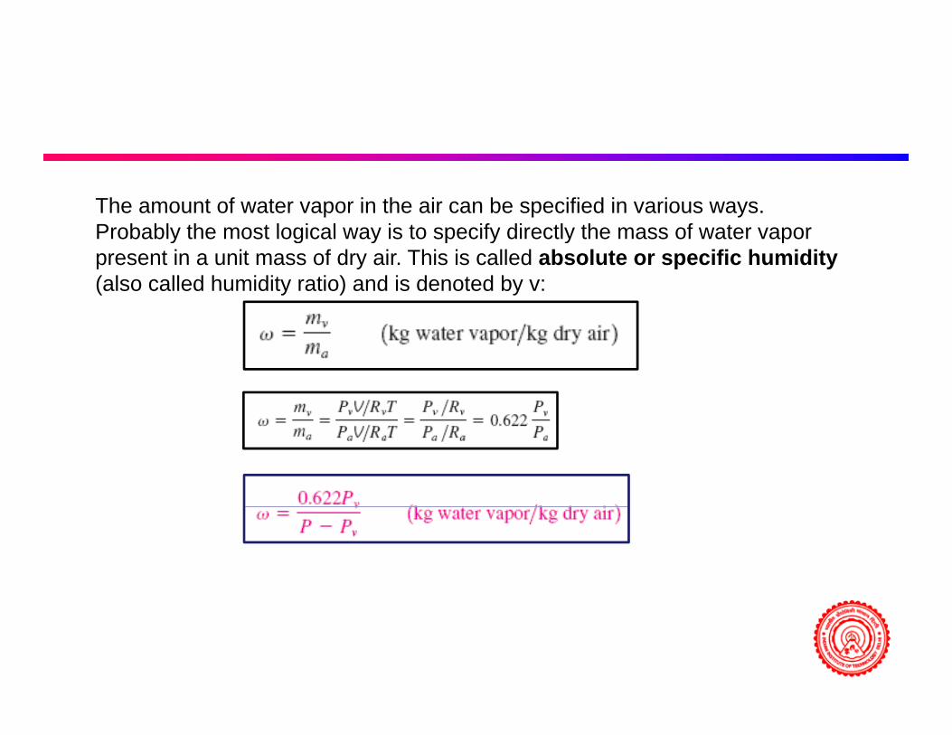
The amount of water vapor in the air can be specified in various ways.Probably the most logical way is to specify directly the mass of water vaporProbably the most logical way is to specify directly the mass of water vaporpresent in a unit mass of dry air. This is called absolute or specific humidity(also called humidity ratio) and is denoted by v:

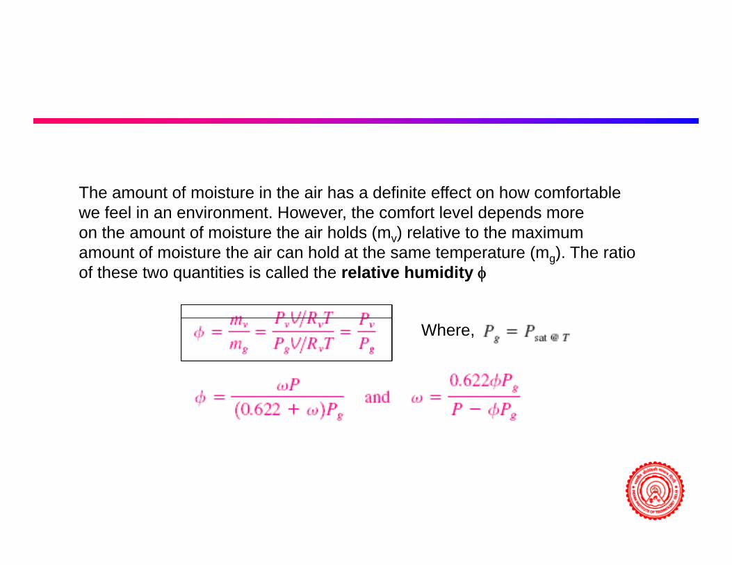
The amount of moisture in the air has a definite effect on how comfortablewe feel in an environment. However, the comfort level depends moreon the amount of moisture the air holds (mv) relative to the maximum

t f i t th i h ld t th t t ( ) Th tiamount of moisture the air can hold at the same temperature (mg). The ratioof these two quantities is called the relative humidity φ

Where,

The total enthalpy (an extensive property) of atmospheric air is the sum of the enthalpies of dry air and the water vapor:the sum of the enthalpies of dry air and the water vapor:

Dividing by m givesDividing by ma gives

Dew point temperaturep p

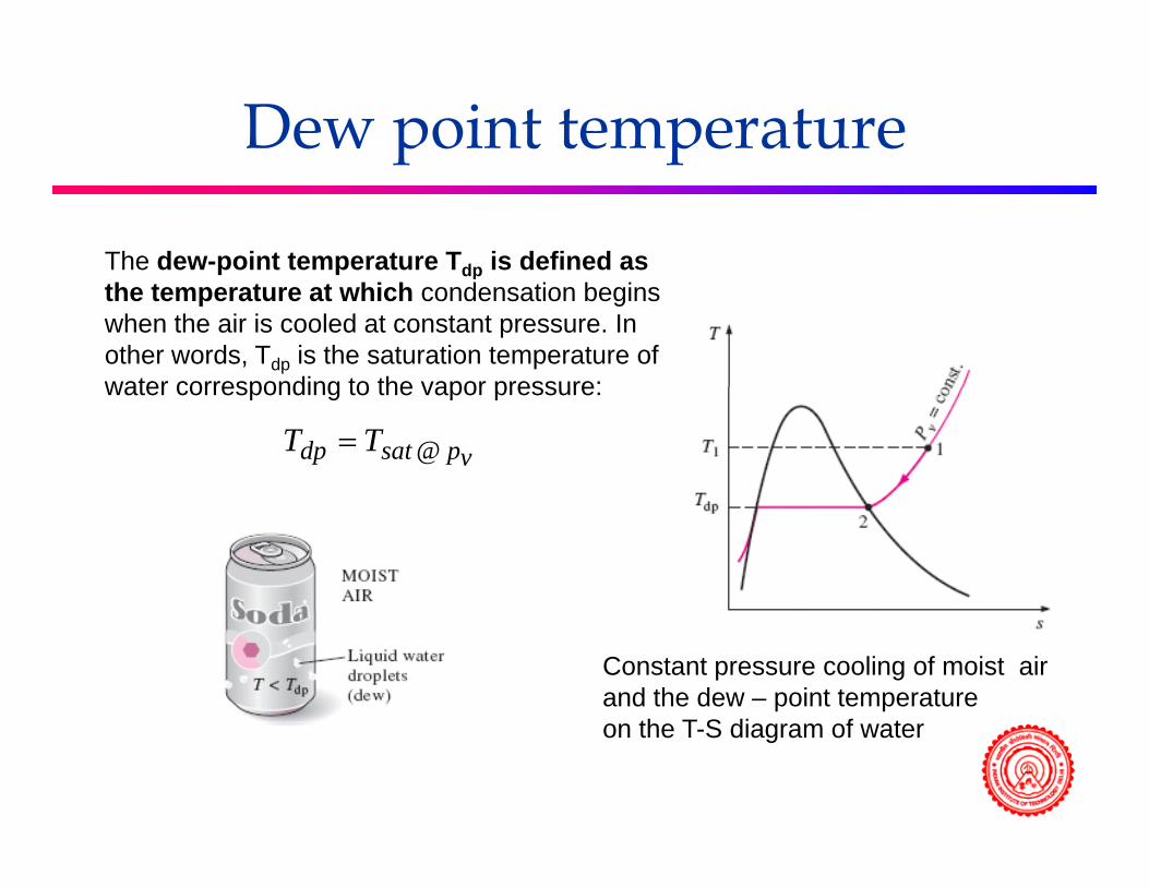
The dew-point temperature Tdp is defined as dpthe temperature at which condensation begins when the air is cooled at constant pressure. In other words, Tdp is the saturation temperature of water corresponding to the vapor pressure:water corresponding to the vapor pressure:

vp@satdp TT =

Constant pressure cooling of moist air and the dew – point temperature

th T S di f ton the T-S diagram of water

Psychrometric Charty

Cooling and dehumidificationg

Hot moist air enters the cooling section at state 1Hot, moist air enters the cooling section at state 1. As it passes through the cooling coils, its temperature decreases and its relative humidityincreases at constant specific humidity. If the cooling section is sufficiently long, air reaches its dew point (state x, saturated air). Further cooling of air results in the condensation of part of the moisture in the air Air remains saturated during themoisture in the air. Air remains saturated during the entire condensation process, which follows a line of 100 percent relative humidity until the final state (state 2) is reached. The water vapor that

d t f th i d i thi icondenses out of the air during this process is removed from the cooling section through a separate channel. The condensate is usuallyassumed to leave the cooling section at T2.g

Mass and Energy Balancegy

The cool, saturated air at state 2 is usually routed directly to the room, where it mixes with the room air. In some cases, however, the air at state 2 may be at the right specific humidity but at a very low temperature Inhumidity but at a very low temperature. In such cases, air is passed through a heating section where its temperature is raisedto a more comfortable level before it is routed to the room.

Problem

Cooling and heating of moist airCooling and heating of moist air• Air enters an air-conditioning unit at 100

kPa 40˚C 70% RH and exists at 100kPa, 40 C, 70% RH, and exists at 100 kPa, 20˚C, 50% RH as shown. The volumetric flow rate at the inlet is 0 25volumetric flow rate at the inlet is 0.25 m3/s. Determine:

The temperature of the air at exit of the cooling unit– The temperature of the air at exit of the cooling unit– The heat transfer rates in the cooling and heating

units

Stepsp

• Write a computer programme for differentWrite a computer programme for different inlet conditions of

Different RH (50 to 90%)– Different RH (50 to 90%).– Different T (say 30 – 60˚C)

• Use curve fit for properties of water –t ti ti (t t b d)saturation properties (temperature based)

Problem

Heat transfer from a cylindrical finHeat transfer from a cylindrical fin• Cylindrical brass rods (4 mm diameter, 5

cm long) are attached to the surface of acm long) are attached to the surface of a power source. Air at 20C is drawn across the rods at 8 m/s Ifthe temperature of thethe rods at 8 m/s. Ifthe temperature of the power source is 60C, find the heattransfer rate from one rod Assume correlations forrate from one rod. Assume correlations for a single rod.

Thermal Insulation

Total Volume of Insulation material:

∫=L

0Wdx)x(tV Wall temperature varies in x -direction

T0

t(x), insulation

∫ ==L Vdx)x(t1t

T(x), Wall surface

∫ ==0

avg LWdx)x(t

Lt

dxT)x(T

kWQL

o∫−&Minimize heat loss through dx)x(t

kWQ0∫=Minimize heat loss through

the insulation

subject to the constraint, V is constant

Optimizationp

dx)x(FL∫=ΦMinimize the

dx)x(WtT)x(T

kW

dx)x(F

Lo

0

∫ ⎥⎤

⎢⎡

λ+−

=

∫=ΦMinimize theheat loss integral

dx)x(Wt)x(t

kW0∫ ⎥

⎦⎢⎣

λ+=

Reduces to 0tF=

∂∂

[ ] 2/12/1

T)x(Tk)x(t ⎟⎞

⎜⎛= ∫ ==

L Vdx)x(t1t

t∂

[ ]oopt T)x(T)x(t −⎟⎠

⎜⎝ λ

=

[ ] 2/1oL

avgopt T)x(T

Lt)x(t −=

∫ ==0

avg LWdx)x(t

Lt

[ ][ ]oL

0

2/1o

opt )(dxT)x(T

)(∫ −

Minimum Heat Transfer Rate

( )2L 2/1kW ⎫⎧& ( )

0

2/1o

avgdxT)x(T

LtkWQ

⎭⎬⎫

⎩⎨⎧∫ −=&

It is worth to mention here that the same expression of t (x) is obtained if the thickness is minimized subjecttopt (x) is obtained if the thickness is minimized subject to a fixed rate of heat loss to the ambient.

Design of heat sink (1-3)g ( )

MEL 806Thermal System Simulation (2-0-2)

Dr. Prabal TalukdarAssociate Professor

Department of Mechanical EngineeringIIT DelhiIIT Delhi

Fins - Recapitulation)TT(hAQ ssconv ∞−=&

There are two ways to increase the rate of heat transfer• to increase the convection heat transfer coefficient h o c e se e co vec o e s e coe c e• to increase the surface area As

• Increasing h may require the installation of a pump or fan, • Or replacing the existing one with a larger onep g g g• The alternative is to increase the surface area by attaching to the surface extended surfaces called fins• made of highly conductive materials such as aluminum• made of highly conductive materials such as aluminum

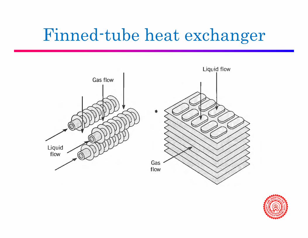
Finned-tube heat exchanger

Longitudinal FinsRectangular Trapezoidal

Triangular Concave parabolicTriangular Concave parabolic

Convex parabolic

Radial Fins

Triangular profile

Rectangular profile

Triangular profile

Hyperbolic profileRadial fin coffee cup

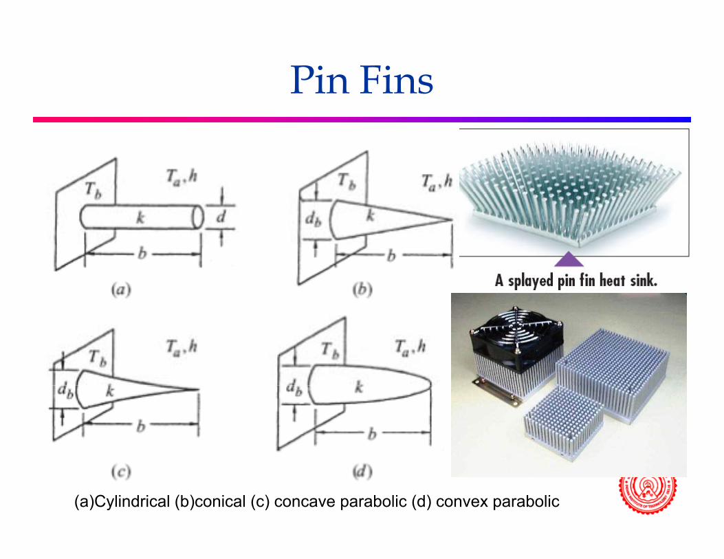
Pin Fins

(a)Cylindrical (b)conical (c) concave parabolic (d) convex parabolic

Plate Fins

The thin plate fins of a car radiator greatly increase the p g yrate of heat transfer to the air

Fins from nature

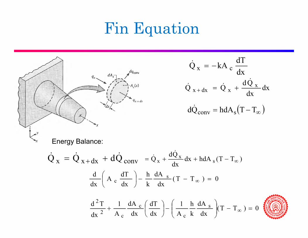
Fin Equation

dxdTkAQ cx −=&dx

dxdxQdQQ x

xdxx&

&& +=+

( )∞−= TThdAQd sconv&

convdxxx QdQQ &&& += +

Energy Balance:

)TT(hdAdxdxQdQ s

xx ∞−++=

&&

dx

0)TT(dx

dAkh

dxdTA

dxd s

c =−−⎟⎠⎞

⎜⎝⎛

∞

0)TT(dx

dAkh

A1

dxdT

dxdA

A1

dxTd s

c

c

c2

2=−⎟⎟

⎠

⎞⎜⎜⎝

⎛−⎟

⎠⎞

⎜⎝⎛+ ∞

Fins with uniform cross sectional area2 ⎞⎛

dA c

0)TT(dx

dAkh

A1

dxdT

dxdA

A1

dxTd s

c

c

c2

2=−⎟⎟

⎠

⎞⎜⎜⎝

⎛−⎟

⎠⎞

⎜⎝⎛+ ∞

0dx

dA c =

PxA s = Pdx

dA s =dx

0)TT(kAhP

dxTd2

2=−⎟⎟

⎠

⎞⎜⎜⎝

⎛− ∞kAdx c ⎠⎝

Excess temperature θ

∞−≡θ T)x(T)x(

d 22θ 0m

dxd 2

2 =θ−θ

(a) Rectangular Fin (b) Pin fin

General Solution and Boundary ConditionsConditions

0d 22

θθ 0m

dx2

2 =θ−

c

2kAhPm =

c

∞−≡θ T)x(T)x(

The general solution is of the form

mx2

mx1 eCeC)x( −+=θ

g

Convection from tip

q denotes Q&q denotes Q

BCs

T)0(T[ ] Lxcc |

dxdTkAT)L(ThA =∞ −=−

bb TT)0(T)0(T

θ≡−=θ=

∞

∞ dx

Lx|dxdk)L(h =θ

−=θ

)xL(msinh)mk/h()xL(mcosh −+−=

θmLsinh)mk/h(mLcoshb +

=θ

Heat Transfer from Fin Surface

0xc0xcbf |dxdkA|

dxdTkAQQ ==

θ−=−== &&

mLcosh)mk/h(mLsinhhPkAQ bcf+

θ=&

dxdx

mLsinh)mk/h(mLcoshhPkAQ bcf +

θ

dA)(hdA]T)(T[hQ θ∫∫•

Another way of finding Q

finAfinAfin dA)x(hdA]T)x(T[hQfinfin

θ∫=−∫= ∞

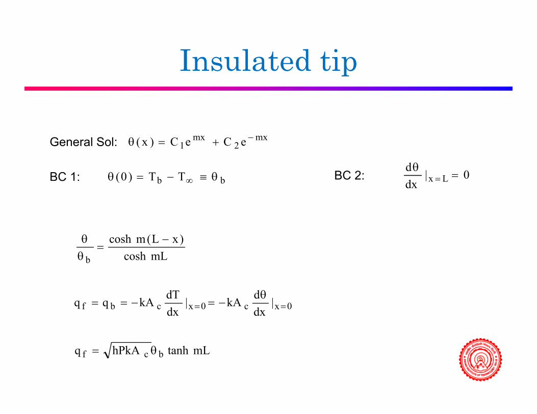
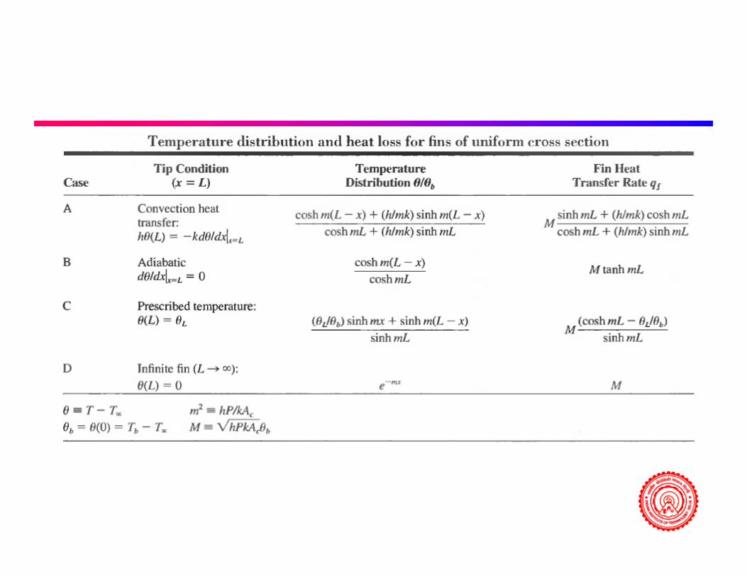
Insulated tip

BC 1: BC 2:

General Sol: mx2

mx1 eCeC)x( −+=θ

bb TT)0( θ≡−=θ ∞ 0|dd

Lx =θ

=C bb)( ∞ |dx Lx

mLcosh)xL(mcosh

b

−=

θθ

0xc0xcbf |dxdkA|

dxdTkAqq ==

θ−=−==

mLtanhhPkAq bcf θ=

Prescribed temperature

This is a condition when the temperature at the tip is known p p(for example, measured by a sensor)

( )mLsinh

)xL(msinhmxsinhbL

b

−+θθ=

θθ

b

( )mLcoshhPkAq bL

bfθθ−

θ=mLsinh

hPkAq bcf θ=

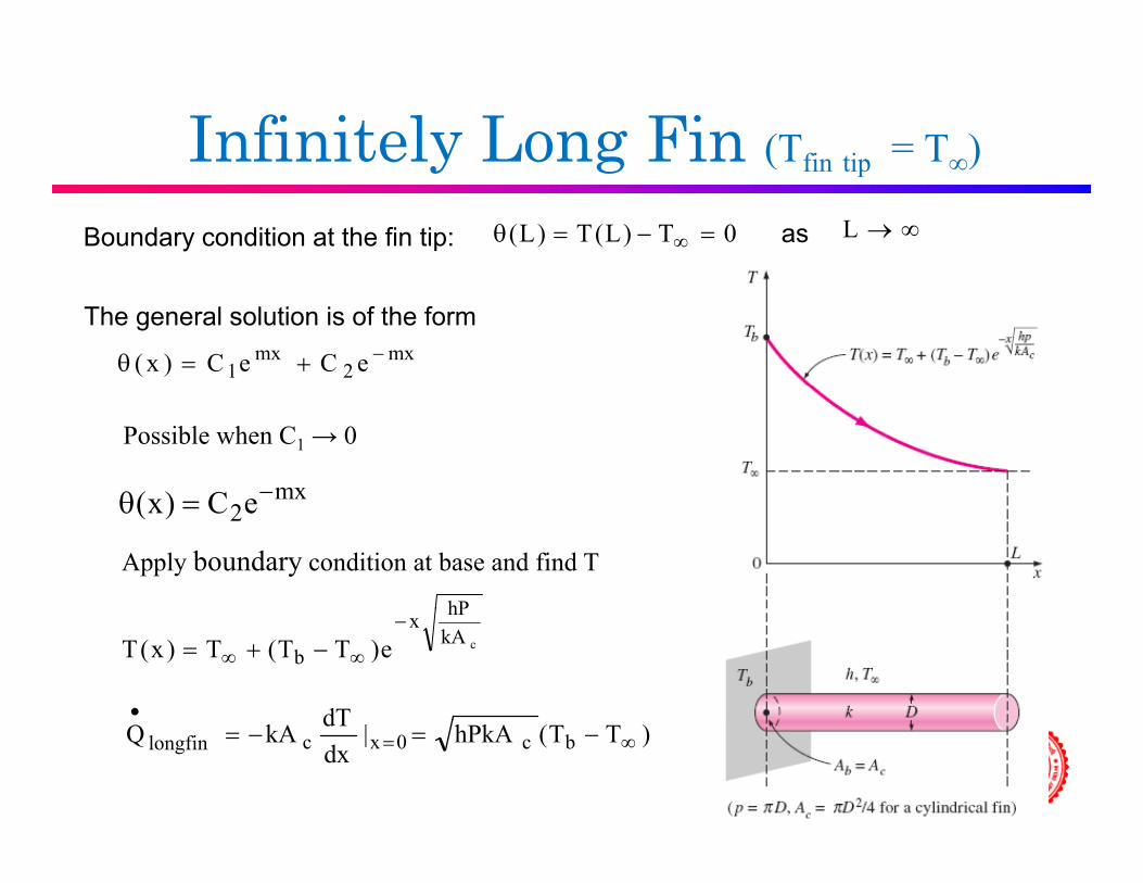
Infinitely Long Fin (Tfin tip = T∞)y g ( fin tip ∞)

Boundary condition at the fin tip: 0T)L(T)L( =−=θ ∞ as ∞→L

mx2

mx1 eCeC)x( −+=θ

The general solution is of the form

Possible when C1 → 0

mxC)( −θ

Apply boundary condition at base and find T

mx2eC)x( =θ

hP

ckAhPx

b e)TT(T)x(T−

∞∞ −+=

dT•)TT(hPkA|

dxdTkAQ bc0xclongfin ∞= −=−=

Corrected fin lengthg

PALL c

c +=Corrected fin length:

Multiplying the relation above by the perimeter gives

Pcg

the perimeter gives Acorrected = Afin (lateral) + Atip

tLL2

LL gularfintanrec,c +=

DLL lfincylindricac +=

Corrected fin length Lc is defined such that heat transfer from a fin of

4lfincylindrica,c

g clength Lc with insulated tip is equal to heat transfer from the actual fin of length L with convection at the fin tip.

Fin Efficiencyy== •

•

finfin

Q

Qη

Actual heat transfer rate from the finIdeal heat transfer rate from the fin

In the limiting case of zero thermal resistance or infinite thermal cond cti it (k ) the temperat re

max,finQ if the entire fin were at base temperature

infinite thermal conductivity (k →∞ ), the temperature of the fin will be uniform at the base value of Tb.

)(••

TThAQQ )(max, ∞−== TThAQQ bfinfinfinfinfin ηη

kATThPkAQcbcfin

l fi11)(

==−

== ∞

•

η

mLmLTThPkAQ

mLhpLTThAQ

bcfin

bfinfin

longfin

tanhtanh)(

)(max,

−

−

∞

•

∞•η

mLmL

TThAmh k

Q

Q

bfin

bc

fin

finipinsulatedt

tanh)(

ta)(

max,

=−

==∞

∞•η

Fin Effectiveness===

•

•

•

)( TThAQQ finfin

finεHeat transfer rate fromthe fin of base area AbHeat transfer rate from− ∞ )( TThAQ bb

nofinHeat transfer rate fromthe surface of area Ab

h kAQ•

)(

cbb

bc

nofin

finlongfin hA

kPTThA

TThPkA

Q

Q=

−−

==∞

∞• )(

)(ε

1. k should be as high as possible, (copper, aluminum, iron). Aluminum is preferred: low cost and weight, resistance to corrosion.p g ,

2. p/Ac should be as high as possible. (Thin plate fins and slender pin fins)

3. Most effective in applications where h is low. (Use of fins justified if when the medium is gas and heat transfer is by natural convection).

Fin Effectiveness••

QQ finfinHeat transfer rate fromth fi f b A=

−==

∞• )( TThA

Q

Q

Q

bb

fin

nofin

finfinε the fin of base area Ab

Heat transfer rate fromthe surface of area Ab

Does not affect the heat transfer at all.1=finεFin act as insulation (if low k material is used)

Enhancing heat transfer (use of fins justified if εfin>2)1

1

>

<

fin

fin

ε

ε

Overall Fin EffectivenessWhen determining the rate of heat transfer from a finned surface, we must consider the ,unfinned portion of the surface as well as the fins. Therefore, the rate of heat transfer for a surface containing n fins can be expressed as

)TT(hA)TT(hA

QQQ

bfinfinbunfin

finunfinfin,total

∞∞

•••

−η+−=

+=

We can also define an overall effectiveness for a finned surface as the

)TT)(AA(h bfinfinunfin ∞−η+=

effectiveness for a finned surface as the ratio of the total heat transfer from the finned surface to the heat transfer from thesame surface if there were no fins

•

)())((

,

,,

∞

∞•

•

−

−+==

TThATTAAh

Q

Q

bnofin

bfinfinunfin

nofintotal

fintotaloverallfin

ηε

Efficiency of circular, rectangular, and triangular fins on a plain surface of width w (from Gardner, Ref 6).

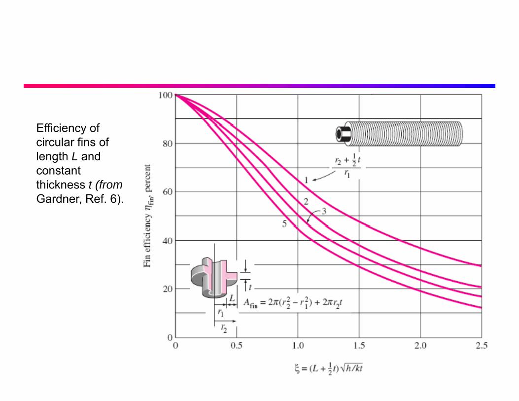
Effi i fEfficiency of circular fins of length L and constant thickness t (fromGardner, Ref. 6).

Proper length of a fin“a” has the same meaning as “m”

ckAhPa =

Optimizationsp

• Maximize heat transfer w r tMaximize heat transfer w.r.t. – Fin thickness t

Profile length b– Profile length b

f• Heat transfer increases asymptotically with increase in thicknessB t h t h ld b th ti thi k if th• But what should be the optimum thickness if the volume (= Ltb) of the fin is constant or the profile area (= bt) is constant?area (= bt) is constant?

Constant Profile Area

Heat transfer from a fin with the adiabatic tipHeat transfer from a fin with the adiabatic tip

Assuming that L>>t and using P ≈ 2Lf c bq hPkA tanh mb= θ

Assuming that L>>t and using P ≈ 2L,

A Lt A bt d tbhPbAc = Lt, Ap = bt and , we get:bkA

mbc

=

h2L

Rearranging:f b

h2Lq h2LkLt tanh bkLt

= θ

h2 2/1⎞⎛ b

kth2tanhtL)hk2(q 2/1

b2/1

f ⎟⎠⎞

⎜⎝⎛θ=

Constant profile areap

• In terms of Ap (= bt)

21

3p21

p21

h2Ak

h2bbA

kh2bb

kAhPmb ⎟

⎠⎞

⎜⎝⎛=⎟

⎠⎞

⎜⎝⎛=⎟

⎠⎞

⎜⎝⎛=⎟

⎟⎞

⎜⎜⎛

=

P ≈ 2L, Ac = Lt

3ppc ktktbtktkA

⎟⎠

⎜⎝

⎟⎠

⎜⎝

⎟⎠

⎜⎝⎟

⎠⎜⎝

11⎞⎛

1/2 1/2f bq (2hk) L t tanh mb= θ

( ) 23p2

1

b2/1

fkt

h2AtanhtLhk2q ⎟⎟⎠

⎞⎜⎜⎝

⎛θ=

( ) 21

3p21

b2/1

fh2AtanhtLhk2q ⎟⎟⎞

⎜⎜⎛

θ= ( ) 3pbfkt

q ⎟⎟⎠

⎜⎜⎝

Optimum conditionp

( ) 21

3p21

b21

f kh2AtanhtLhk2q ⎟⎠⎞

⎜⎝⎛θ= h2 2/1

⎞⎛( ) 3pbf kt

q⎠⎝ b

kth2tanhtL)hk2(q 2/1

b2/1

f ⎟⎠⎞

⎜⎝⎛θ=

( )1122f bq 2hk L t tanh= θ β

0dt

dqf =

Atkh2mb where2sinh6 p

232/1

⎟⎠⎞

⎜⎝⎛==ββ=β

−

1.4192k

=β⎠⎝

Gives optimum fin efficiency to be 0.627

Optimum conditionp

• Let us name profile fin length and fin thickness to be bo and to for theLet us name profile fin length and fin thickness to be bo and to for the optimum condition

• Substituting Ap = boto in h2 32/1 −⎞⎛ At

kh2mb p

2−

⎟⎠⎞

⎜⎝⎛==β

31/2• We get,32

1/2

o o o o2h mb t b t k

−⎛ ⎞β = = ⎜ ⎟⎝ ⎠

For constant profile area

Solving for to yields optimum fin thickness

22/1 ⎞⎛

Solving for bo yields theoptimum fin profile length

2/1

For constant profile area

bkh2t

2o

2/1

o ⎟⎟⎠

⎞⎜⎜⎝

⎛β

⎟⎠⎞

⎜⎝⎛=

h2ktb

2/1o

o ⎟⎠⎞

⎜⎝⎛β=

Constant heat transfer from a fin• If the heat transfer rate is constant

β( )111 222f b p 3

2hq 2hk L t tanh A Lkt

⎛ ⎞= θ ⎜ ⎟⎝ ⎠ β

tanh tanh1.4192 0.8894β = =

⎝ ⎠

• Solving for t gives the optimum fin thickness to for constant heat transfer from a fin

2q⎛ ⎞f

o 1/2b

2

qt

(2hk) w 0.8894

0 632

⎛ ⎞⎜ ⎟=⎜ ⎟θ⎝ ⎠

⎛ ⎞

L2

0 632 ⎛ ⎞fo 2

b

q0.632thkw

⎛ ⎞= ⎜ ⎟

θ⎝ ⎠ p 0 0A b t=Because,f

o 2b

q0.632thkL

⎛ ⎞= ⎜ ⎟

θ⎝ ⎠

Optimum valuep122h⎛ ⎞Si

0 o0

2hm b bkt

⎛ ⎞β = = ⎜ ⎟

⎝ ⎠Since,

1 12k⎛ ⎞2 2

0 okb t

2h⎛ ⎞= β⎜ ⎟⎝ ⎠

Re-arranging,

2fq0 632 ⎛ ⎞f

o 2b

q0.632thkL

⎛ ⎞= ⎜ ⎟

θ⎝ ⎠11 2 22 f

0 2qk 0.632b 1.4192

⎛ ⎞⎛ ⎞⎛ ⎞ ⎜ ⎟= ⎜ ⎟⎜ ⎟ ⎜ ⎟⎝ ⎠0 2

bb 1.4192

2h hkL ⎜ ⎟⎜ ⎟ ⎜ ⎟θ⎝ ⎠ ⎝ ⎠⎝ ⎠

fq0.798b f0

b

qbhL

=θ

Constant fin volume or mass

• The volume of the fin is V = Lbt• And profile area is Ap = bt = V/L• Since , the width L is not a parameter this problem is

basically the same as the constant profile area.

( ) 21

321

b21

fh2VtanhtLhk2q ⎟⎠⎞

⎜⎝⎛⎟⎠⎞

⎜⎝⎛θ= ( )

121

21

3bf

h2bh2

ktLq

−⎞⎛⎟⎞

⎜⎛

⎟⎠

⎜⎝⎟⎠

⎜⎝

20

2

00

02

000 t

kh2

LtbbV

kth2bmb ⎟

⎠⎞

⎜⎝⎛=⎟⎟

⎠

⎞⎜⎜⎝

⎛==β

Optimum length and thicknessp g

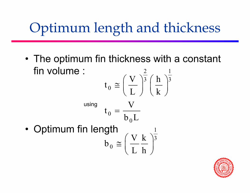
• The optimum fin thickness with a constantThe optimum fin thickness with a constant fin volume : 2 1

3 3V ht ⎛ ⎞ ⎛ ⎞≅ ⎜ ⎟ ⎜ ⎟0tL kVt

≅ ⎜ ⎟ ⎜ ⎟⎝ ⎠ ⎝ ⎠

using

• Optimum fin length

00

1

tb L

=

⎛ ⎞p g

30

V kbL h

⎛ ⎞≅ ⎜ ⎟⎝ ⎠

Multiple Fin Array Ip y

• Free (Natural) Convection CoolingFree (Natural) Convection Cooling– For a single fin, the consideration is given to

the thickness and length of the fin to get thethe thickness and length of the fin to get the maximum heat transfer rate.

– Additional consideration for fin array: finAdditional consideration for fin array: fin spacing z and number of fins n for a given plate area L x W

• In general, the thickness of fin is usually much smaller than the fin spacing z.

Small Spacing Channelp g

• Consider a small hot parallel plate channel with constant p pwall temperature To.

• Cold air at T∞ enters through the bottom of the channel by natural convection.

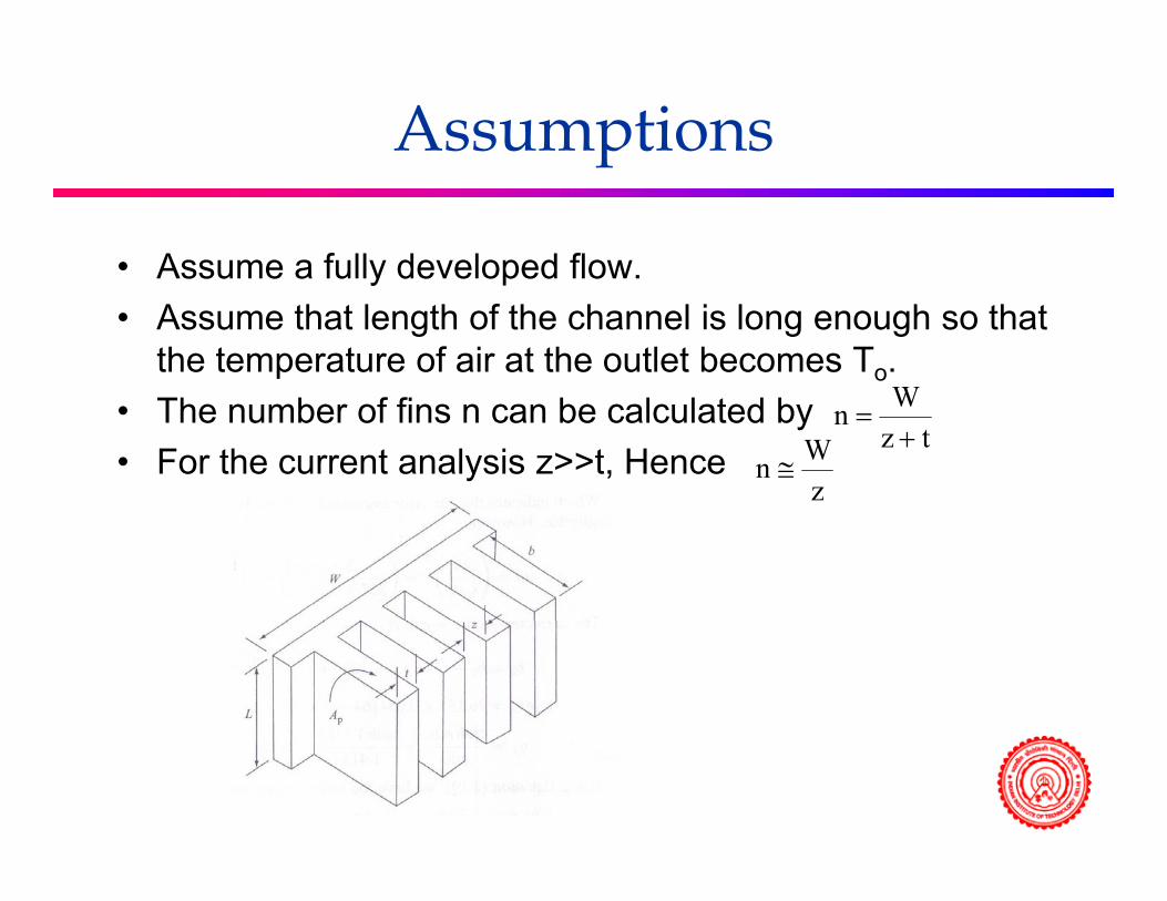
Assumptionsp

• Assume a fully developed flow.y p• Assume that length of the channel is long enough so that

the temperature of air at the outlet becomes To.W• The number of fins n can be calculated by

• For the current analysis z>>t, Hence

Wnz t

=+Wn

z≅

Momentum Equationq

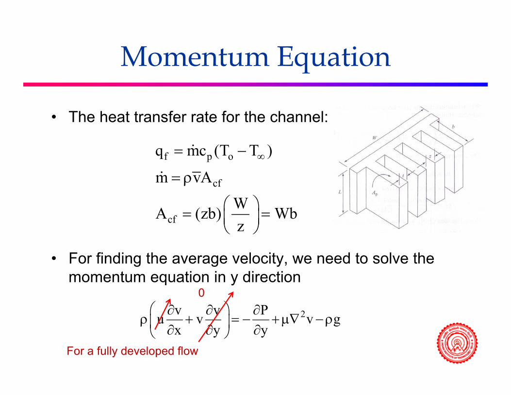
• The heat transfer rate for the channel:

f p oq mc (T T )

A∞= −&

& cf

cf

m vAWA (zb) Wb

= ρ

⎛ ⎞= =⎜ ⎟⎝ ⎠

&

• For finding the average velocity, we need to solve the t ti i di ti

cf z⎜ ⎟⎝ ⎠

momentum equation in y direction

2v v Pu v v g⎛ ⎞∂ ∂ ∂

ρ + = − +μ∇ −ρ⎜ ⎟

0

u v v gx y y

ρ + +μ∇ ρ⎜ ⎟∂ ∂ ∂⎝ ⎠For a fully developed flow

Pressure Gradient

• Since both ends of the channel are open, the pressure p , pgradient is given by: P g

y ∞∂

= −ρ∂

• So, the momentum equation becomes:2

2v0 ( g) g∞

∂= − −ρ +μ −ρ

∂ 2

2

2

y

( )gvy

∞

∂

ρ −ρ∂= −

μ∂ 1 ∂ρ⎛ ⎞Thermal expansion coeff.

• The Boussinesq approximation:y μ∂

(T T )ρ ρ = ρ β

P

1T∂ρ⎛ ⎞β = − ⎜ ⎟ρ ∂⎝ ⎠

(T T )∞ ∞ ∞ρ −ρ = ρ β −

Average velocityg y

• Using Boussinesq approximation:

2o

2g (T T )v

y∞β −∂

= −ν∂

Constant

Integrate twice with B.C. (i) no slip and (ii) symmetry at the centerline

2og (T T ) xv 18 z / 2

∞⎡ ⎤β − ⎛ ⎞= −⎢ ⎥⎜ ⎟ν ⎝ ⎠⎢ ⎥⎣ ⎦8 z / 2ν ⎝ ⎠⎢ ⎥⎣ ⎦

Upon integrating this along the spacing z, the average velocity can be calculated:

2og (T T )zv12

∞β −=

νg y 12ν

Mass Flow Rate

m vA= ρ&

2g (T T )zβ

cf

cf

m vAA Wb= ρ

=

o

2o

g (T T )zv12

g (T T )z Wb

∞

∞

β −=

νρ β −

&

Average velocity

og ( )m Wb12

∞ρ β=

ν

f p oq mc (T T )∞= −&

Mass flow rate

f p oq ( )∞

2 2o

f ,small Pg (T T ) zq c Wb

12∞β −

= ρν

Heat transfer fromfin array with

2f ,small

12q z

ν∝

fin array with small spacing

Large spacing channelg p g• Consider a large spacing, a large enough for

h b d l t b i l t d b teach boundary layer to be isolated between isothermal plates Th N lt b f t l ti i i• The Nusselt number for natural convection in air for a vertical plate

Lh

Wh th R l i h b i d fi d

25.0L

airRa517.0

KLhNu ==

Where the Rayleigh number is defined as( ) 3

0L

g T T LRa ∞β −

=να

Heat Transfer Equationq• In above equation RaL is the Rayleigh number

(f fl l t f l th L) β i th(for a flow over a plate of length L) , β is the volumetric expansion coefficient, α is the thermal diffusivity and g is gravitydiffusivity, and g is gravity.

• The volumetric expansion coefficient β =1/TfWhere Tf is the film temperatureWhere Tf is the film temperature

• Using Newton’s law of cooling, the heat transfer rate fins for the large channels can be written asrate fins for the large channels can be written as

( )∞−= TThAq 0seargl,f ( )0seargl,f

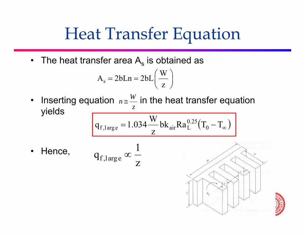
Heat Transfer Equationq• The heat transfer area As is obtained as

W⎛ ⎞

• Inserting equation in the heat transfer equation

sWA 2bLn 2bLz

⎛ ⎞= = ⎜ ⎟⎝ ⎠

Wn ≅Inserting equation in the heat transfer equation yields z

n ≅

( )∞−= TTRabkz

W034.1q 025.0

Laireargl,f

• Hence,

z

f ,larg e1qz

∝z

Optimum Fin Spacingp p g

• The optimal spacing can be obtained byThe optimal spacing can be obtained by equations of heat transfers

earglfsmallf qq = eargl,fsmall,f qq

( ) 414

13

0opt R32LTTg32z −

−

∞ ⎥⎤

⎢⎡ −β( ) 4

L0opt Ra3.2g3.2

L∞ =⎥

⎦⎢⎣ ανβ

≅

Forced Convection Coolingg

• Small spacing channel– Flow between parallel plates in the case of a smallFlow between parallel plates in the case of a small

spacing channel is known as Couett-Poiseulli flow.

Small spacing channelp g

• The x-momentum equation:The x momentum equation:2 2

2 2u u P u uu v v

⎛ ⎞⎛ ⎞∂ ∂ ∂ ∂ ∂ρ + = − +μ +⎜ ⎟⎜ ⎟∂ ∂ ∂ ∂ ∂⎝ ⎠ ⎝ ⎠

0

For a fully developed flow

Th di t l th h l i

2 2x y x x y⎜ ⎟∂ ∂ ∂ ∂ ∂⎝ ⎠ ⎝ ⎠

• The pressure gradient along the channel is constant: P P∂ Δ

=

• Momentum equation reduces tox L∂

2

2u P

L∂ Δ

μ =∂

q 2 Ly∂

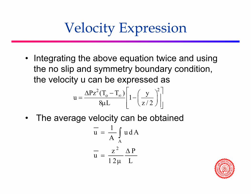
Velocity Expressiony p

• Integrating the above equation twice and usingIntegrating the above equation twice and using the no slip and symmetry boundary condition, the velocity u can be expressed as

22oPz (T T ) yu 1

8 L z / 2∞

⎡ ⎤Δ − ⎛ ⎞= −⎢ ⎥⎜ ⎟μ ⎝ ⎠⎢ ⎥⎣ ⎦

• The average velocity can be obtained 1u u d A= ∫

A2

u u d AA

z Pu Δ=

∫

1 2 Lμ

Heat Transfer from Fin

The heat transfer rateThe heat transfer rate( )∞−= TTcmq 0psmall,f &

⎟⎠⎞

⎜⎝⎛⎟⎟⎠

⎞⎜⎜⎝

⎛μΔ

ρ=zWzb

L12pzm

2&

( )2

f ,small p 0z pq Wb c T T12 L ∞Δ

= ρ −μ

2small,f zq ∝

Large Spacing Channelg p gAssumption:

C id l i h l• Consider a large spacing channel• Each boundary layer is isolated• The pressure drop is assumed to be constant• For laminar flow the Nusselt and Reynolds number

i itt f P 0 5is written as for Pr >0.5

31

21

PR6640LhN 32L

airL PrRe664.0

KNu ==

∞LUReν

=ReL

Heat Transfer Equationq• Heat transfer equation

( )TThAq ( )

( )∞

∞

−=

−=

TTRePr664.0L

kbLW2q

TThAq

021

31

aireargl,f

0seargl,f

( )

( )∞∞

∞

−⎟⎠⎞

⎜⎝⎛= TTLUPrbkW328.1q

Lzq

021

31

airearglf

0eargl,f

• Since ∆P was assumed to be constant, U∞ may

( )∞⎟⎠

⎜⎝ ν

bz

3 8.q 0aireargl,f

be expressed in terms of ∆P and z• Considering the shear stress is the root cause of

h d l h f b l (the pressure drop, apply the force balance (next page)

Heat Transfer Equationq

( ) ( )WbPbLW2 Δ=⎟⎠⎞

⎜⎝⎛τ

The coefficient of friction for laminar flow

( ) ( )z⎟⎠

⎜⎝

21

L2

f Re328.1U1C

−

=ρ

τ=

32

⎟⎞

⎜⎛

Eliminating the τ

Heat transfer equation

U2 ∞ρ 3

21

21

L328.1

PzU⎟⎟⎟

⎠

⎞

⎜⎜⎜

⎝

⎛

νρ

Δ=∞

q

( )∞

−

−⎟⎟⎠

⎞⎜⎜⎝

⎛ρνΔ

= TTzPLPrWbk208.1q 0323

1

2aireargl,f⎠⎝ ρν

32

eargl,f zq−

∝2

small,f zq ∝

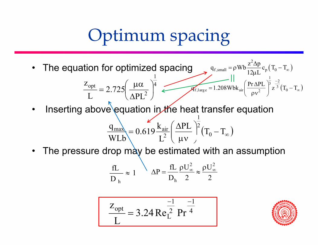
Optimum spacingp p g

• The equation for optimized spacing1

( )2

f ,small p 0z pq Wb c T T12 L ∞Δ

= ρ −μ

I ti b ti i th h t t f ti

41

2opt

PL725.2

Lz

⎟⎠⎞

⎜⎝⎛Δμα

= ( )∞

−

−⎟⎟⎠

⎞⎜⎜⎝

⎛ρνΔ

= TTzPLPrWbk208.1q 0323

1

2aireargl,f

• Inserting above equation in the heat transfer equation

( )∞−⎟⎟⎠

⎞⎜⎜⎝

⎛μνΔ

= TTPLLk619.0

WLbq

021

2airmax

• The pressure drop may be estimated with an assumption ⎠⎝ μνLWLb

fL UUfL 22 ρρ1

DfL

h≈

11

2U

2U

DfLP

h

∞∞ ρ≈

ρ=Δ

41

21

Lopt PrRe24.3L

z −−

=

Multiple Fin Array IIp y

s,f c bq hPkA tanh(mb)= θHeat transferfrom a single fin

p cwhere, A bt, A Lt, P 2L and mb= = ≅ β =1/2hp 2h⎛ ⎞

from a single fin

c

hp 2hmkA kt

⎛ ⎞= = ⎜ ⎟⎝ ⎠

s,f b

1/2

q h(2L)k(Lt) tanh= θ β

⎛ ⎞1/2

ps,fb

2hkAqtanh

L b⎛ ⎞

= θ β⎜ ⎟⎝ ⎠

Heat transfer from base wall

• Consider heat transfer rate q at the baseConsider heat transfer rate qw at the base wall between two fins

w w bq h LzAW W

= θ

pAW Wz tn n b

= − = −

⎛ ⎞pww b

Aq WhL n b

⎛ ⎞= θ −⎜ ⎟

⎝ ⎠Where, n is number of fins

Total heat transfer from fin

• The total heat transfer rate from the multiple fin array is:p y

q h(2L)k(Lt) tanh= θ β

w w b

p

q h LzAW Wt

= θ

s,f b

1/2ps,f

b

q h(2L)k(Lt) tanh

2hkAqtanh

= θ β

⎛ ⎞= θ β⎜ ⎟

p

pwb

z tn n b

Aq Wh

= − = −

⎛ ⎞= θ −⎜ ⎟b tanh

L bθ β⎜ ⎟

⎝ ⎠w bh

L n bθ ⎜ ⎟⎝ ⎠

1/2p ptotal

b w b2hkA Aq Wn tanh h

L b n b

⎡ ⎤⎛ ⎞ ⎛ ⎞⎢ ⎥= θ β+ θ −⎜ ⎟ ⎜ ⎟⎢ ⎥⎝ ⎠ ⎝ ⎠⎣ ⎦L b n b⎢ ⎥⎝ ⎠ ⎝ ⎠⎣ ⎦

Expression for single finp gTo find the maximum total heat transfer with respect to b, we set the derivative equal to zeroq

totaldq 0db

=And finally obtained an expression:

2 2 w2h btanh 3 sec hk

β β− β β =And finally obtained an expression:

If h is ass med to be ero e get optim m β for a single fin2 2tanh 3 sec h 0

3 sinh coshβ β− β β =β β β

If hw is assumed to be zero, we get optimum β for a single fin

3 sinh coshβ = β β

sinh 2 2sinh cosh6 sinh 2

β = β ββ = β

Using

6 sinh 21.4192

β = ββ =

Solve to get

Optimum βp

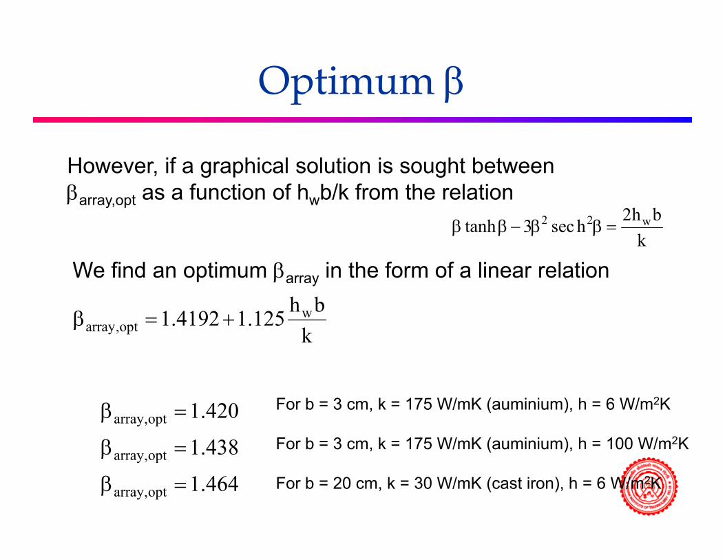
However, if a graphical solution is sought between, g p gβarray,opt as a function of hwb/k from the relation

2 2 w2h btanh 3 sec hk

β β− β β =k

wh b1 4192 1 125β +

We find an optimum βarray in the form of a linear relation

warray,opt 1.4192 1.125

kβ = +

438.1

420.1

optarray

opt,array

=β

=β For b = 3 cm, k = 175 W/mK (auminium), h = 6 W/m2K

For b = 3 cm, k = 175 W/mK (auminium), h = 100 W/m2K

464.1opt,array

opt,array

=β

β

For b = 20 cm, k = 30 W/mK (cast iron), h = 6 W/m2K

Natural Convection Coolingg

Elenbass suggested optimum Nusselt number for two vertical plate as

opt

opt optu

fluid

h zN 1.25

k= =

fluidopt

opt

kh 1.25z

=

O i i l fi h f i h 1 4192

( ) ( )11

s,f 2 22 b bq

2hkt tanh 1 258 h A k= θ β = θ

Optimum single fin heat transfer with β = 1.4192

( ) ( )20 b b p2hkt tanh 1.258 h A kL

= θ β = θ

( )1qq q W ⎛ ⎞⎛ ⎞

Total optimum heat transfer rate from the fin array is bww zh

Lq

θ=

( )s,f 2total 2b opt p opt opt b

opt 0

qq q Wn 1.258 h A k h zL L L z t

ω⎛ ⎞⎛ ⎞

= + = θ + θ⎜ ⎟⎜ ⎟ ⎜ ⎟+⎝ ⎠ ⎝ ⎠

Optimum heat transferpUsing

h2

ktb 2/1

oo ⎟

⎠⎞

⎜⎝⎛β=

opt

fluid

zk

opt 25.1h = 41

Lopt Ra32

z −

=h2 ⎠⎝ opt

41

Lopt

L

Ra714.2L

z

Ra3.2L

−

=

=

Bar -Cohen and Rohsenow

1

Lwith Ap = boto

14

12

fluid 0fluid

k kt0.8063 1.25kRa Lq −

⎛ ⎞⎜ ⎟ +⎜ ⎟⎝ ⎠ where4

Ltotal1

b 4L 0

Ra LqLW

2.714Ra L t−

⎜ ⎟⎝ ⎠=

θ+ ( )0

Lg T T L

Raβ −

=αν

where

αν

Optimum spacingp p g

Assuming the heat transfer from the interfin area between the fins is negligible, following Eq.

( )1

s,f 2total 2b opt p opt opt b

opt 0

qq q Wn 1.258 h A k h zL L L z t

ω⎛ ⎞⎛ ⎞

= + = θ + θ⎜ ⎟⎜ ⎟ ⎜ ⎟+⎝ ⎠ ⎝ ⎠

( )12

opt 0total1.258 h ktq

≅

opt 0⎝ ⎠ ⎝ ⎠

simplifies to

b opt 0LW z t≅

θ +

Diff i i h b E d i h d i iDifferentiating the above Eq. w.r.t. to and setting the derivative to zero provides the optimum spacing for the maximized heat transfer rate

tz ≅ oopt tz ≅

Problem

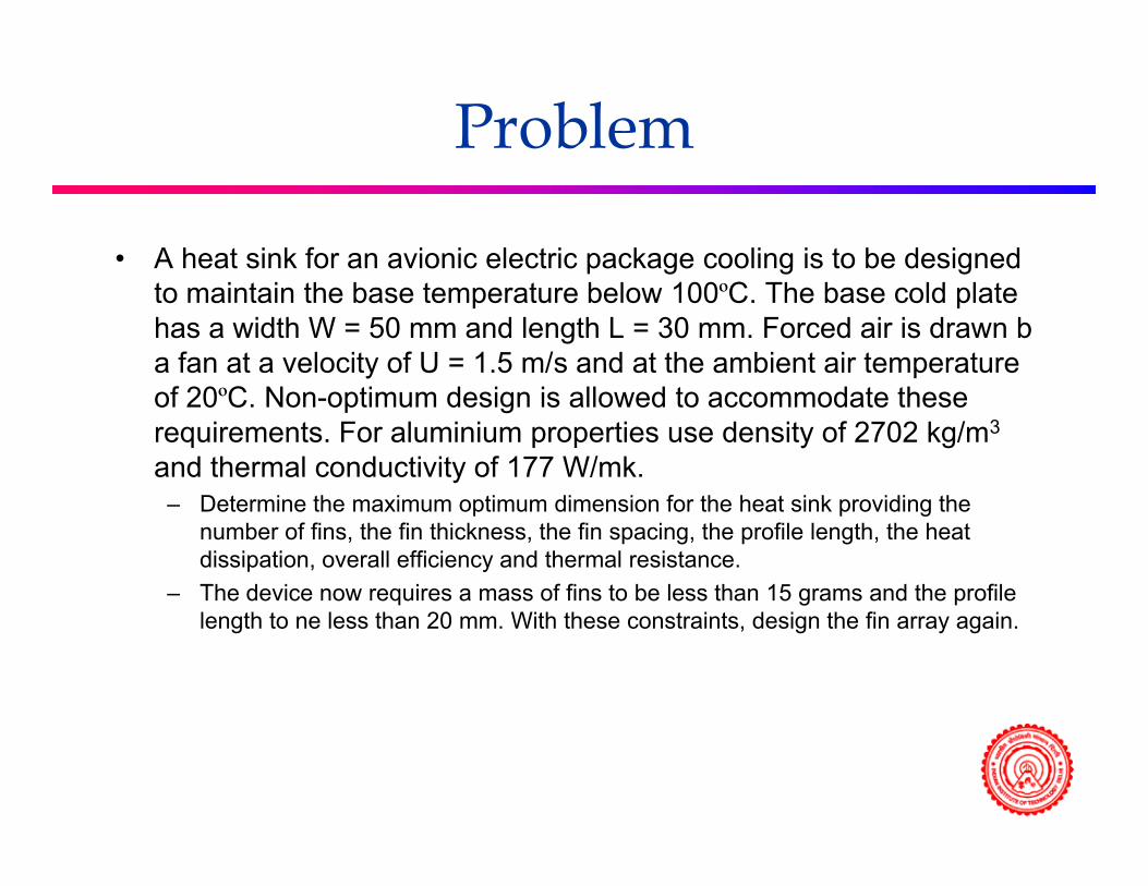
• A heat sink for an avionic electric package cooling is to be designed to maintain the base temperature below 100ºC. The base cold plate has a width W = 50 mm and length L = 30 mm. Forced air is drawn b a fan at a velocity of U = 1.5 m/s and at the ambient air temperature f 20 C N ti d i i ll d t d t thof 20ºC. Non-optimum design is allowed to accommodate these

requirements. For aluminium properties use density of 2702 kg/m3

and thermal conductivity of 177 W/mk.D t i th i ti di i f th h t i k idi th– Determine the maximum optimum dimension for the heat sink providing the number of fins, the fin thickness, the fin spacing, the profile length, the heat dissipation, overall efficiency and thermal resistance.

– The device now requires a mass of fins to be less than 15 grams and the profile length to ne less than 20 mm. With these constraints, design the fin array again.

• Find 41

21

opt PR243z −−

Find • Find hL

A β f i l fi

42L

opt PrRe24.3L

=

• Assume β for a single fin.• Optimize heat transfer rate as a function of

to.• Find

h2ktb

2/1o

o ⎟⎠⎞

⎜⎝⎛β=

• Volume of a fin Val(to)=Lboto• Number of fins n (t )=W/(z + t )

h2 ⎠⎝

• Number of fins nf(to)=W/(zopt + to)

• Total mass of the fin array as a function of to mal(to)=nf(to)ρalVal(to)

• Heat transfer rate from a single fin• Heat transfer rate from the interfin area• Total heat transfer rate• Fin effectiveness• Total area• Total area• Overall surface efficiency• Overall thermal resistance

PLATE-FIN HEAT EXCHANGER

Prabal TalukdarPrabal TalukdarAssociate Professor

Department of Mechanical EngineeringDepartment of Mechanical EngineeringIIT Delhi

E-mail: [email protected]

Mech/IITD

Basic componentBasic componentThis type of extended surface heat exchanger has corrugated fins mostly of triangular or rectangular cross-sections sandwiched between the parallel plates

Mech/IITD

Different types of plate finDifferent types of plate fin

Mech/IITD

Mech/IITD

Plate-fin with OSPPlate fin with OSP

Mech/IITD

Plate–fin heat exchangerPlate fin heat exchanger• Plate –fin heat exchangers have various geometriesPlate  fin heat exchangers have various geometries in order to compensate for the high thermal resistance, particularly if one of the fluid is gas.

• The plate fins are categorized as triangular fin, rectangular fin, wavy fin, offset strip fin (OSP), louvered fin, and perforated fin

• Generally used for moderate operating pressures less h k ( )than 700 kPa (gauge pressure)

• It has a surface area density of up to 5900 m2/m3.

Mech/IITD

• Common fin thickness ranges between 0 05 toCommon fin thickness ranges between 0.05 to 0.25 mm.

• Fin height may range from 2 to 25 mm• Fin height may range from 2 to 25 mm• Typical fin densities are 120 to 700 fins/m, but 

ld h 2100 fi /could reach to 2100 fins/m

Mech/IITD

Geometrical CharacteristicsGeometrical Characteristics• Single‐pass crossflow plate heat exchanger isSingle pass crossflow plate heat exchanger is considered.

Mech/IITD

Total number of passagesTotal number of passages• The number of passages for the hot fluid sideThe number of passages for the hot fluid side and cold fluid side are Np and Np + 1. 

• The top and bottom passage are designated to• The top and bottom passage are designated to be cold fluid.Th b f b b i d• The number of passages can be obtained as:

w1PN22b1PN1bpN3L δ++++= ⎟⎟⎠

⎞⎜⎜⎝

⎛⎟⎠⎞

⎜⎝⎛

w22b3LN

δ−−

⎠⎝⎠⎝

Length of fluid 1 Length of fluid 2 Thickness of total plates

Mech/IITD

w22b1b23pN

δ++=Solving for Np

No of finsNo of fins

• The total number of fins for fluid 1 (hot):

pN1fp1L

1fn = where pf1 is fin pitch.

• The total number of fins for fluid 2 (cold):⎞⎛2L

Mech/IITD

⎟⎠

⎞⎜⎝

⎛ += 1pN2fp2

2fn

Primary AreaPrimary Area• Primary area for fluid 1 is:Primary area for fluid 1 is:

⎟⎟⎠

⎞⎜⎜⎝

⎛⎟⎟⎠

⎞⎜⎜⎝

⎛ +δ+++δ−= 1pN1Lw22b2PN2L1b21fn2L2pN2L1L21pA

Total plate area Fin base area Passage side wall area Passage front and back wall areaback wall area

Mech/IITD

No of offset strip finsNo. of offset strip fins• The number of offset strip fins per the numberThe number of offset strip fins per the number of fins is obtained from:

21

2 λL

offn =

12

1

2

λL

offn =

Where λ1 2 is the offset strip fin length for fluid 

1

1,2  p g1 and 2.

Mech/IITD

Total Fin AreaTotal Fin Area• The total fin area consists of the fin area Af1 and offset‐strip 

edge areas:edge areas:

1121111111

212121 fnfPfn

offn

fPfnoffnbfnLbfA δδδδδδ +−−+−+−=

⎟⎟⎟

⎠

⎞

⎜⎜⎜

⎝

⎛

⎟⎟⎟

⎠

⎞

⎜⎜⎜

⎝

⎛

⎟⎟⎠

⎞⎜⎜⎝

⎛⎟⎟⎠

⎞⎜⎜⎝

⎛

⎠⎝⎠⎝

Fin surface areas Offset-strip edge areas Internal offset – strip edge area(d-e and g-f) 2(b-c-d-e) 2(i-j-k-l-i)(d e and g f) 2(b c d e) 2(i j k l i)

First and last offset – strip edge area2(a-b-i-j-a)

Mech/IITD

Total heat transfer areaTotal heat transfer area• The total heat transfer area isThe total heat transfer area is 

1fA1pA1tA +=

• The free flow (cross sectional) area Ac1 is

⎞⎛⎞⎛

• The frontal area for fluid 1 where

1fn1fP1b1cA ⎟⎟⎠

⎞⎜⎜⎝

⎛⎟⎠

⎞⎜⎝

⎛ δ−δ−=

• The frontal area for fluid 1 wherefluid 1 is entering is defined by 

Mech/IITD

3L1L1frA =

Fin efficiencyFin efficiency• The hydraulic diameter:

A2L1cA4

1hD =

• For the fin efficiency ηf of the offset strip fin, it is assumed that the heat flow from both plates is uniform and that the 

1tA1h

padiabatic plate occurs at the middle of the plate spacing b1. Hence the profile length Lf1 is defined by  δ−= 2

1b1fL

• The m value is obtained as:

2

⎟⎟⎟⎟

⎠

⎞

⎜⎜⎜⎜

⎝

⎛

λδ+

δ=

11

fkh2

1m

⎟⎞

⎜⎛ Lt h

• The single fin  efficiency is⎟⎟

⎠⎜⎜

⎝=

AfLm

fLm

fη11

11tanh

• The overall fin efficiency is Mech/IITD

⎟⎟⎟

⎠

⎞

⎜⎜⎜

⎝

⎛−−=

ft

Af

A

o ηη 11

111

Optimum-Insulationsp

MEL 806Thermal System Simulation (2-0-2)

Dr. Prabal TalukdarAssociate Professor

Department of Mechanical EngineeringIIT DelhiIIT Delhi

Thermal Insulation

Total Volume of Insulation material:

∫=L

0Wdx)x(tV Wall temperature varies in x -direction

T0

t(x), insulation

∫ ==L Vdx)x(t1t

T(x), Wall surface

∫ ==0

avg LWdx)x(t

Lt

dxT)x(T

kWQL

o∫−&Minimize heat loss through dx)x(t

kWQ0∫=Minimize heat loss through

the insulation

subject to the constraint, V is constant

Optimizationp

dx)x(FL∫=ΦMinimize the

dx)x(WtT)x(T

kW

dx)x(F

Lo

0

∫ ⎥⎤

⎢⎡

λ+−

=

∫=ΦMinimize theheat loss integral

dx)x(Wt)x(t

kW0∫ ⎥

⎦⎢⎣

λ+=

Reduces to 0tF=

∂∂

[ ] 2/12/1

T)x(Tk)x(t ⎟⎞

⎜⎛= ∫ ==

L Vdx)x(t1t

t∂

[ ]oopt T)x(T)x(t −⎟⎠

⎜⎝ λ

=

[ ] 2/1oL

avgopt T)x(T

Lt)x(t −=

∫ ==0

avg LWdx)x(t

Lt

[ ][ ]oL

0

2/1o

opt )(dxT)x(T

)(∫ −

Variational Calculas

• Consider a Integral given as ∫ ′=b

dx)y,y,x(FIConsider a Integral given as Where y(x) is a function of x

• The special function y(x) for which the integral I reaches

a

an extremum satisfies the Euler equtaion,

0=⎟⎟⎠

⎞⎜⎜⎝

⎛′∂

∂−

∂∂ F

ddF

• If the wanted variable y(x) additionally satisfies an integral constraint of the type,

⎟⎠

⎜⎝ ′∂∂ ydxy

bintegral constraint of the type,

• Then y(x,λ) satisfies the new Euler equation

∫ ′=a

dx)y,y,x(GC

⎞⎛ where H = F + λG0=⎟⎟⎠

⎞⎜⎜⎝

⎛′∂

∂−

∂∂

yH

dxd

yH

Minimum Heat Transfer Rate

( )2L 2/1kW ⎫⎧& ( )

0

2/1o

avgdxT)x(T

LtkWQ

⎭⎬⎫

⎩⎨⎧∫ −=&

It is worth to mention here that the same expression of t (x) is obtained if the thickness is minimized subjecttopt (x) is obtained if the thickness is minimized subject to a fixed rate of heat loss to the ambient.

Modeling of Thermal Systemsg y

MEL 806Thermal System Simulation (2-0-2)

Dr. Prabal TalukdarAssociate Professor

Department of Mechanical EngineeringIIT DelhiIIT Delhi

Modelingg

• The process of simplifying a given problem soThe process of simplifying a given problem so that it may be represented in terms of a system of equations for analysis or a physicalof equations, for analysis, or a physical arrangement, for experimentation, is termed modelingmodeling

• The design and optimization processes are closely coupled with the modeling effort andclosely coupled with the modeling effort, and the success of the final design is very strongly influenced by the accuracy and validity of theinfluenced by the accuracy and validity of the model employed.

Descriptive Modelp

• The model may be descriptive or predictive. • We are all very familiar with models that are used to

describe and explain various physical phenomena. A working model of an engineering system such as aworking model of an engineering system, such as a robot, an internal combustion engine, a heat exchanger, or a water pump, is often used to explain how the device

kworks. • Frequently, the model may be made of clear plastic or

may have a cutaway section to show the internalmay have a cutaway section to show the internal mechanisms.

• Such models are known as descriptive and are frequently d i l t l i b i h i dused in classrooms to explain basic mechanisms and

underlying principles

Predictive model

• Predictive models are of particular interest to our present p ptopic of engineering design because these can be used to predict the performance of a given system.Th ti i th li f h t t l• The equation governing the cooling of a hot metal sphere immersed in an extensive cold-water environment represents a predictive model because it allows us to obtain the temperature variation with time and determine the dependence of the cooling curve on physical variables such as initial temperature of thephysical variables such as initial temperature of the sphere, water temperature, and material properties

Modeling g

• Physical insight is the main basis for the simplification of y g pa given system to obtain a satisfactory model. Such insight is largely a result of experience in dealing with a variety of thermal systemsvariety of thermal systems.

• Estimates of the underlying mechanisms and different effects that arise in a given system may also be used to simplify and idealize. Knowledge of other similar processes and of the appropriate approximations employed for these also helps in modelingemployed for these also helps in modeling.

• Overall, modeling is an innovative process based on experience, knowledge, and originality.

Experimentp

• In many practical systems, it is not possible toIn many practical systems, it is not possible to simplify the problem enough to obtain a sufficiently accurate analytical or numerical solution. In such cases, experimental data are obtained, with help from dimensional analysis to d t i th i t t di i ldetermine the important dimensionless parameters.

• Experiments are also crucial to the validation of• Experiments are also crucial to the validation of the mathematical or numerical model and for establishing the accuracy of the results obtainedestablishing the accuracy of the results obtained

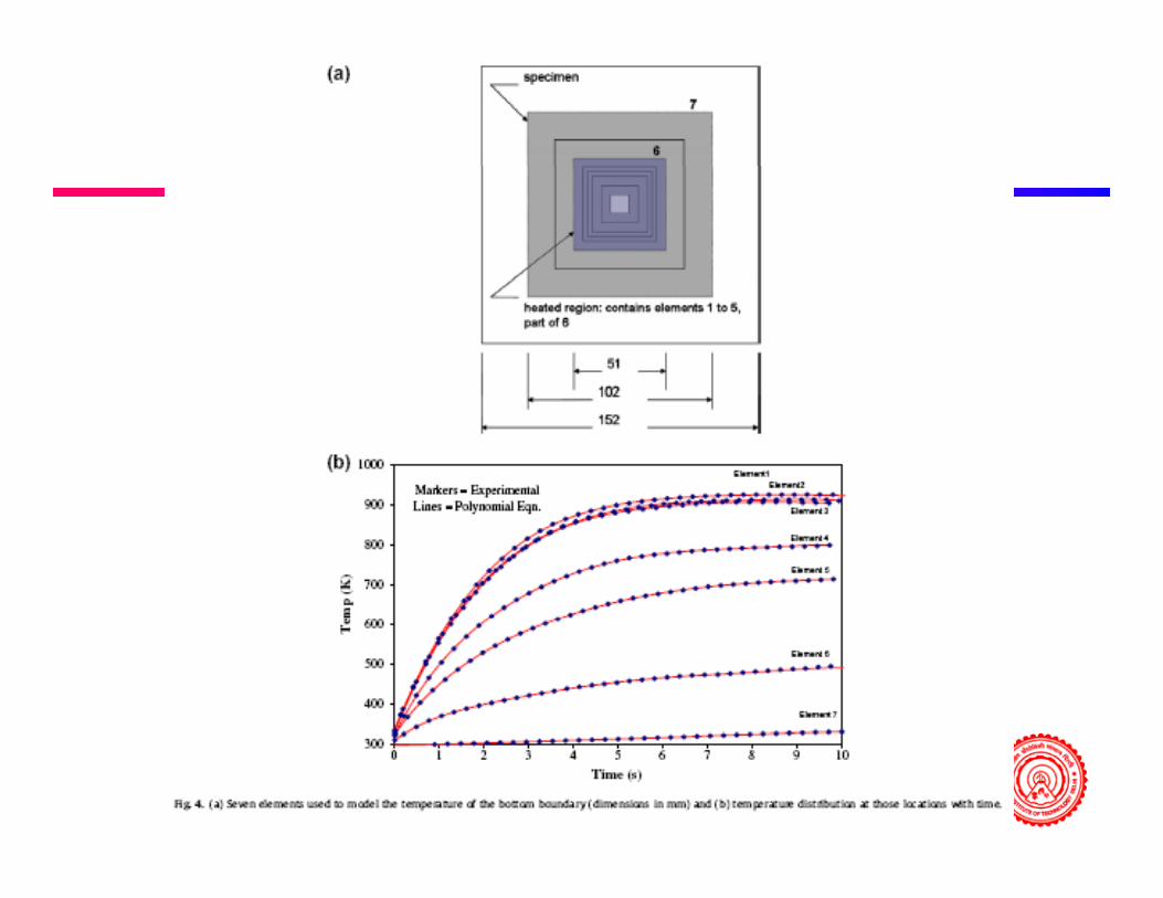
Fire Protective Fabrics

Modeling of the setupg p

Points selected for temperature measurements of entire specimen holder.

Curve-fittingg• Material properties are usually available as discrete data

at various values of the independent variable, e.g.,at various values of the independent variable, e.g., density and thermal conductivity of a material measured at different temperatures. For all such cases, curve fitting is frequently employed to obtain appropriate correlatingis frequently employed to obtain appropriate correlating equations to characterize the data. These equations can then serve as inputs to the model of the system, as well as to the design process.

Types of Modelyp

• Analog modelsAnalog models• Mathematical models

Ph i l d l• Physical models• Numerical models

Analog Modelg

• Analog models are based on the analogy or similarity g gy ybetween different physical phenomena and allow one to use the solution and results from a familiar problem to obtain the corresponding results for a different unsolvedobtain the corresponding results for a different unsolved problem.

• An example of an analog model is provided by conduction heat transfer through a multilayered wall, which may be analyzed in terms of an analogous electric circuit with the thermal resistance represented by thecircuit with the thermal resistance represented by the electrical resistance and the heat flux represented by the electric current

Examples of Analog Modelp g

Conduction heat transfer in a composite wall Analog model of plumeConduction heat transfer in a composite wall Analog model of plume . flow in a room fire

Mathematical Model• A mathematical model is one that represents the

performance and characteristics of a given system inperformance and characteristics of a given system in terms of mathematical equations.

• These models are the most important ones in the design p gof thermal systems because they provide considerable versatility in obtaining quantitative results that are needed as inputs for designas inputs for design.

• Mathematical models form the basis for numerical modeling and simulation, so that the system may be investigated without actually fabricating a prototype

• A solution to the equations for a heat exchanger would give the dependence of the total heat transfer rate on thegive the dependence of the total heat transfer rate on the inlet temperatures of the two fluids and on the dimensions of the system.

Physical Modely

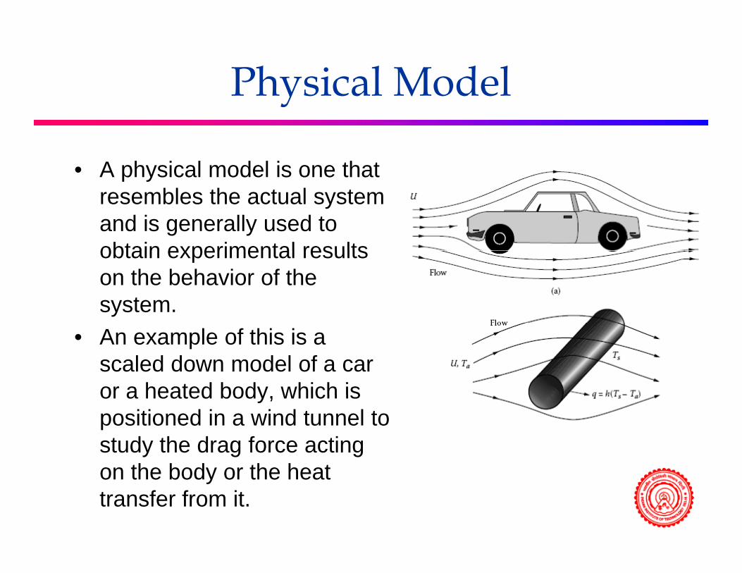
• A physical model is one that p yresembles the actual system and is generally used to obtain experimental resultsobtain experimental results on the behavior of the system.

• An example of this is a scaled down model of a car or a heated body which isor a heated body, which is positioned in a wind tunnel to study the drag force acting

th b d th h ton the body or the heat transfer from it.

Numerical Model

• Numerical models are based on mathematicalNumerical models are based on mathematical models and allow one to obtain, using a computer, quantitative results on the system behavior for different operating conditions and design parameters.

• Numerical modeling refers to the restructuring and discretization of the governing equations in order to solve them on a computer The relevantorder to solve them on a computer. The relevant equations may be algebraic equations, ordinary or partial differential equations integralor partial differential equations, integral equations, or combinations of these.

Interaction between models

• Even though the four main types of modeling of g yp gparticular interest to design are presented as separate approaches, several of these frequently overlap in practical problemspractical problems.

• Experimental data from physical models may indicate some of the approximations or simplifications that may be used in developing a mathematical model.

• Although numerical modeling is based largely on the mathematical model outputs from the physical or analogmathematical model, outputs from the physical or analog models may also be useful in developing the numerical scheme.

Classification of models

• There are several other classifications ofThere are several other classifications of modeling frequently used to characterize the nature and type of the modelthe nature and type of the model.

• Steady state or dynamic, • deterministic or probabilistic,deterministic or probabilistic, • lumped or distributed, and • Discrete or continuous.

For instance, the model for a hot-water storage system may be described as a dynamic, continuous, lumped, deterministic mathematical model. Similarly, the mathematical model for a furnace may be specified as steady state, continuous, distributed, and deterministic

Mathematical Modelingg

• The development of a mathematical modelThe development of a mathematical model requires physical understanding, experience and creativity it is oftenexperience, and creativity, it is often treated as an art rather than a science.

• Inputs for Model development• Inputs for Model development• Knowledge of existing systems,• characteristics of similar systems• characteristics of similar systems,• governing mechanisms, and • commonly made approximations and idealizationsy pp

Steps in Model Developmentp p

• Transient/steady stateTransient/steady state• Spatial dimensions• Lumped mass approximationsLumped mass approximations• Simplifications of boundary conditions• Negligible effects• Negligible effects• Idealizations• Material Properties• Material Properties• Conservation laws

F th i lifi ti f i ti• Further simplifications of governing equations

Transient/steady statey

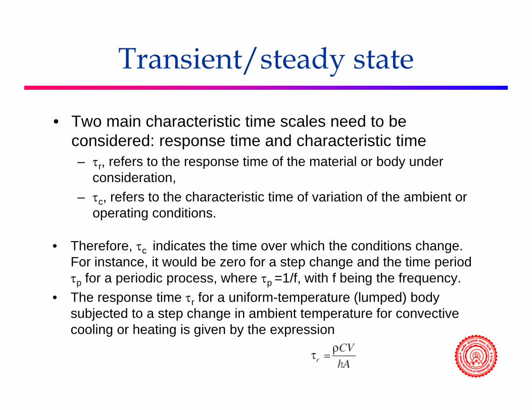
• Two main characteristic time scales need to be considered: response time and characteristic time – τr, refers to the response time of the material or body under

considerationconsideration, – τc, refers to the characteristic time of variation of the ambient or

operating conditions.

• Therefore, τc indicates the time over which the conditions change. For instance, it would be zero for a step change and the time period τp for a periodic process, where τp =1/f, with f being the frequency. τp p p , τp , g q y

• The response time τr for a uniform-temperature (lumped) body subjected to a step change in ambient temperature for convective cooling or heating is given by the expressiong g g y p

Response, characteristic timep• τc is very large, τc →∞.

In this case, the conditions may be assumed to remain unchanged with time and the system may be treated as steady state.steady state.

• τc << τr. In this case, the operating conditions change very rapidly, as compared to the response of the material. Then the material is unable to follow the variations in the operating variables.operating variables.

An example of this is a deep lake whose response time is very large compared to the fluctuations in the ambient medium. Even though the surface temperature may reflect the effect of such fluctuations, the bulk p yfluid would essentially show no effect of temperature fluctuations. Then the system may be approximated as steady with the operating condition taken at their mean values

Response, characteristic timep

• τc >> τr

This refers to the case where the material or body responds very fast but the operating or boundary conditions change very slowly. An example of this is the slow variation of the solar flux with time on a sunny day and the rapid response of the collectorand the rapid response of the collector

Replacement of the ambient temperature variation with time by a finite number of steps, with the temperature held constant over each stepover each step

Periodic processp• Periodic processes: In many cases, the behavior

f th th l t b t dof the thermal system may be represented as a periodic process, with the characteristics repeating over a given time period τrepeating over a given time period τp.

• Environmental processes are examples of this modeling because periodic behavior over a daymodeling because periodic behavior over a day or over a year is of interest in many of these systems.

The net heat transfer over the cycle must be zero because, if it is not, there is a net gain or loss of energy. This would result in a consequent increase or decrease of temperature with time and a cyclic behavior would not be obtained

Transient Process

• If none of the previous approximations is applicable, the p pp pp ,system has to be modeled as a general time-dependent problem. Th ti l t ti l l i• There are many practical systems, particularly in materials processing, that require such a dynamic model because transient effects are crucial in determining the quality of the product and in the control and operation of the system.

• Heat treatment and metal casting systems are examples• Heat treatment and metal casting systems are examples in which a transient model is essential to study the characteristics of the system for design.

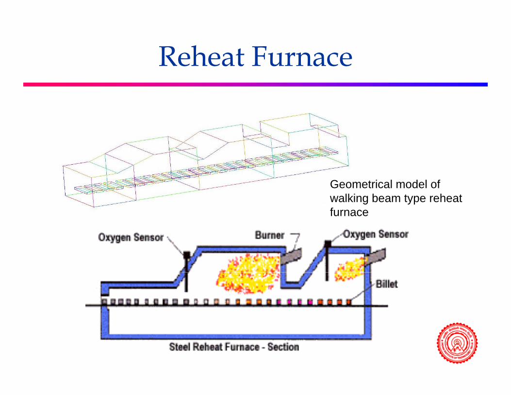
Reheat Furnace

Geometrical model of walking beam type reheat furnace

Spatial Dimensionsp

• Though all practical systems are three-dimensional, they g p y , ycan often be approximated as two - or one-dimensional to considerably simplify the modeling. Thus, this is an important simplification and is based largely on theimportant simplification and is based largely on the geometry of the system under consideration and on the boundary conditions.

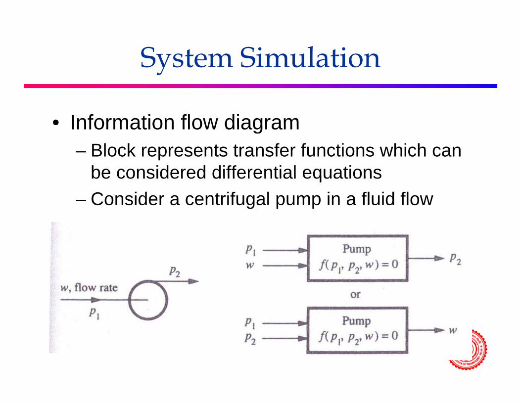
System Simulationy

• Information flow diagramInformation flow diagram– Block represents transfer functions which can

be considered differential equationsbe considered differential equations– Consider a centrifugal pump in a fluid flow

Fire water facilityy

w

at3AA ppCw −=

The equations for the water flow rate through open hydrants are :

at3AA pp

at4BB ppCw −=

Equationsq

The equations for the pipe section 0-1 is :

ghwCpp 2 ρ+= ghwCpp 111at ρ+=−

21232 wCpp =−Pipe section 2-3:

22343 wCpp =−Pipe section 3-4:

System of Equationsy q

• These five equations can be written in functional form:q

0)pw(f0)p,w(f 3A1 =

0)p,w(f0)p,w(f

113

4B2

==

0)p,p,w(f0)p,p,w(f

4325

3214

==

• An additional function is provided by the pump characteristics: 0)ppw(f

)pp( 4325

= 0)p,p,w(f 2116 =

Six equations – eight unknowns??

Information-flow diagramg

• Mass balances provide the other twoMass balances provide the other two equations

• and0)w,w,w(f www 2A172A1 =+=

0)ww(fww• and 0)w,w(f ww B28B2 ==

Sequential and Simultaneous CalculationsCalculations

S ti it i ibl t t t ith th i t• Sometimes it is possible to start with the input information and immediately calculate the output of a component. The output information from this first component is all that is needed to calculate the input information of the next component and so on to the final component of the system This is a sequentialcomponent of the system. This is a sequential calculation

• In simultaneous calculations, a set of algebraic equations need to be solved simultaneously.

Modeling of Thermal Systemsg y

MEL 806Thermal System Simulation (2-0-2)

Dr. Prabal TalukdarAssociate Professor

Department of Mechanical EngineeringIIT DelhiIIT Delhi

Examplep

• A water pumping station consists of two parallel pumps p p g p p pdrawing water from a lower reservoir and delivering it to another that is 40 m higher. In addition to overcoming the pressure difference due to elevation the friction inthe pressure difference due to elevation, the friction in the pump is 7.2w2, where w is combined flow rate in kilograms per second. The pressure-flow-rate

fcharacteristics of the pumps are2

1 12

p 810 25w 3.75w

900 65 30

Δ = − −

ΔWhere w1 and w2 are the flow rate through pump 1 and pump 2, respectively. Use successive substitution to

22 2p 900 65w 30wΔ = − −

p p p ysimulate the system and determine the values of Δp, w1,w2, w.

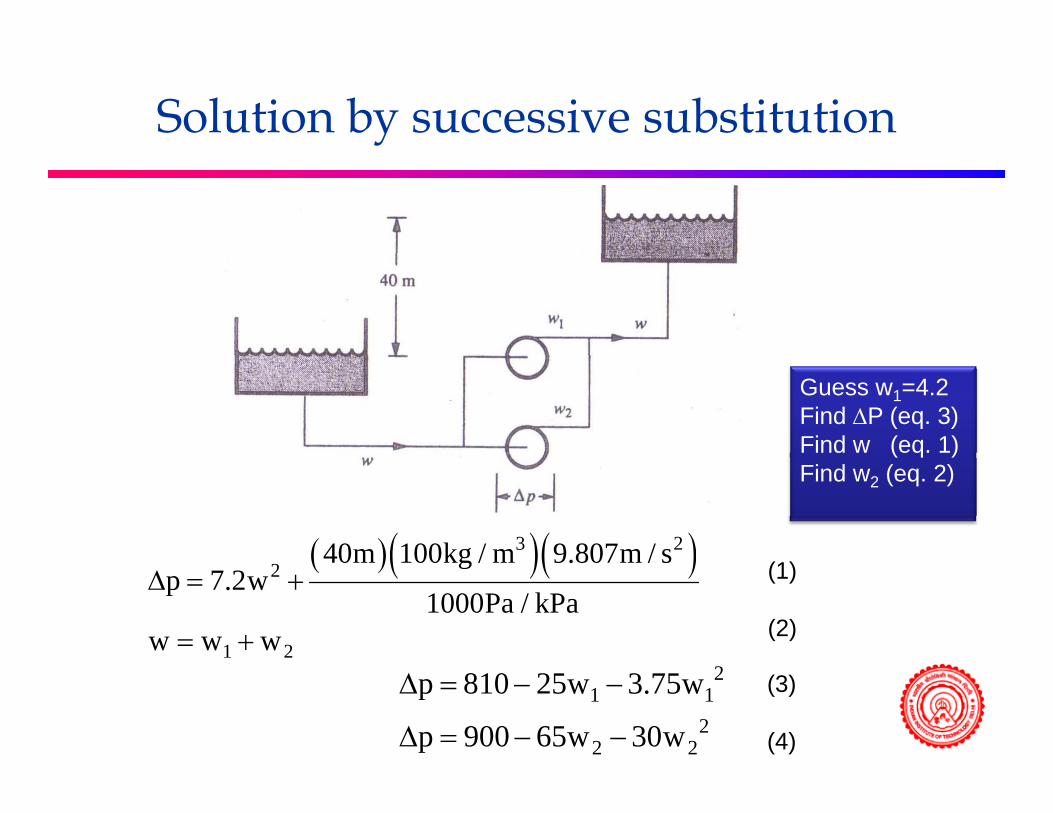
Solution by successive substitution

Guess w1=4.2Find ΔP (eq. 3)Find w (eq. 1)

( )( )( )3 240m 100kg / m 9.807m / s

Find w2 (eq. 2)

( )( )( )2

1 2

40m 100kg / m 9.807m / sp 7.2w

1000Pa / kPaw w w

Δ = +

= +

(1)

(2)

21 1

22 2

p 810 25w 3.75w

p 900 65w 30w

Δ = − −

Δ = − −

(3)

(4)

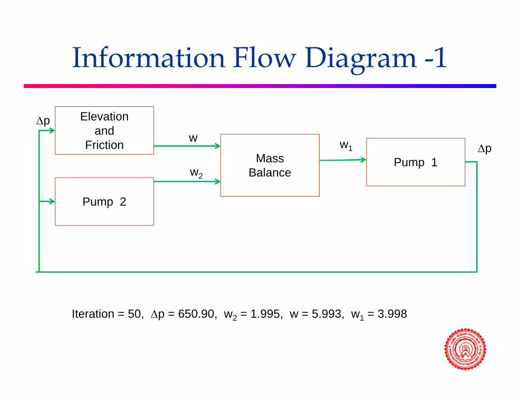
Information Flow Diagram -1g

ElevationΔpand

FrictionMass

BalancePump 1

w

w2

w1

p

Δp

Balance

Pump 2

2

Iteration = 50, Δp = 650.90, w2 = 1.995, w = 5.993, w1 = 3.998

Information Flow Diagram - 2g

ElevationΔpand

FrictionMass

BalancePump 2

w

w1

w2

p

Δp

Balance

Pump 1

1

Start with w2 = 2.0 DivergesIteration = 5 Δp = 42 8 w = imaginaryIteration = 5, Δp = 42.8, w = imaginary

Information Flow Diagram - 3g

ΔpPump 1

Mass Balance

Elevationand

Friction

w1

w2

w

p

Δp

Balance Friction

Pump 2

2

Start with w = 6.0 DivergesIteration = 9 Δp = 951 2 w = imaginaryIteration = 9, Δp = 951.2, w1 = imaginary

Newton-Raphson Methodp

Taylor series expansion:

)ax(d

)a(yd21)ax(

d)a(dy)a(yy 2

2

2−−−+−⎥

⎦

⎤⎢⎣

⎡+−+=

Taylor series expansion:

)ax)](a(y[)a(yydx2dx 2

−′+≈

⎥⎦

⎢⎣

Basis of Newton-Raphson iterative techniqueq

e2x)x(y

e2xx

x

−+=

=+ Solve

0)x(ye2x)x(y

c =+

Xc is the correct value of x that solves the eq.

Assume some temporary value of x, say xt = 2

y(xt) = -3.39

Newton-Raphson Methodp

E i t f b di b tExpress y in terms of x by expanding about x

)xx)](x(y[)x(y)x(y cc −′+≈

)xx)](x(y[)x(y)x(y tcttc −′+≈For x = xt

0

)x(y)x(y

xxt

ttc ′−≈

)x(y t

Newton-Raphson method with multiple eqs. and unknownsunknowns

• Suppose that three nonlinear equations to beSuppose that three nonlinear equations to be solved for the three unknown variables x1, x2, x3.

f1(x1,x2,x3) = 01( 1, 2, 3)f2(x1,x2,x3) = 0f3(x1 x2 x3) = 0f3(x1,x2,x3) 0

• Rewrite the equations so that all terms are on one side of the equality signo e s de o t e equa ty s g

• Assume temporary values for the variables, x1,t, x2 t and x3 t2,t 3,t

Algorithmg

• Calculate the values of f1, f2 and f3 at the temporary 1, 2 3 p yvalues of x1, x2 and x3.

• Compute the partial derivatives of all functions with t t ll i blrespect to all variables.

• Use Taylor-series expansion to establish a set of simultaneous equationssimultaneous equations

)()x,x,x(f

)()x,x,x(f

)x,x,x(f)x,x,x(f

t3t2t11t3t2t11

c,3c,2c,11t,3t,2t,11

∂∂

≈

)xx()x,x,x(f

)xx(x

),,()xx(

x),,(

t,3t,2t,11

c,2t,22

t,3t,2t,11c,1t,1

1

t,3t,2t,11

∂+

−∂

+−∂

+

)xx(x c,3t,3

3

,,, −∂

+

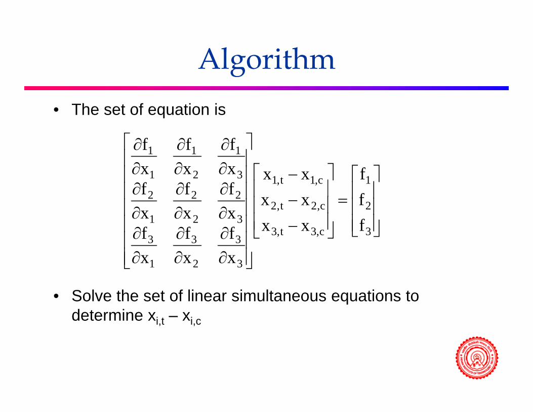
Algorithmg• The set of equation is

⎤⎡⎥⎤

⎢⎡ −⎥⎥⎤

⎢⎢⎡

∂∂

∂∂

∂∂

1c1t13

1

2

1

1

1

fxxxf

xf

xf

⎥⎥⎥

⎦

⎤

⎢⎢⎢

⎣

⎡=

⎥⎥⎥

⎦

⎤

⎢⎢⎢

⎣

⎡

−−

⎥⎥⎥⎥⎥

⎢⎢⎢⎢⎢

∂∂∂∂∂

∂∂

∂∂

3

2

1

c3t3

c,2t,2

c,1t,1

3

2

2

2

1

2

ff

xxxx

fffxf

xf

xf

⎦⎣⎦⎣

⎥⎥⎦⎢

⎢⎣ ∂

∂∂∂

∂∂ 3c,3t,3

3

3

2

3

1

3

xf

xf

xf

• Solve the set of linear simultaneous equations to determine xi,t – xi,c

Algorithmg

• Correct the x’sCorrect the x s• X1,new = x1,old – (x1,t – x1,c)

----------• X3,new = x3,old – (x3,t – x3,c)

• Test for convergence. If the absolute magnitudes of all the f’s or all the Δx’s aremagnitudes of all the f s or all the Δx s are satisfactorily small, terminate: Otherwise return to step (indicated with red)p ( )

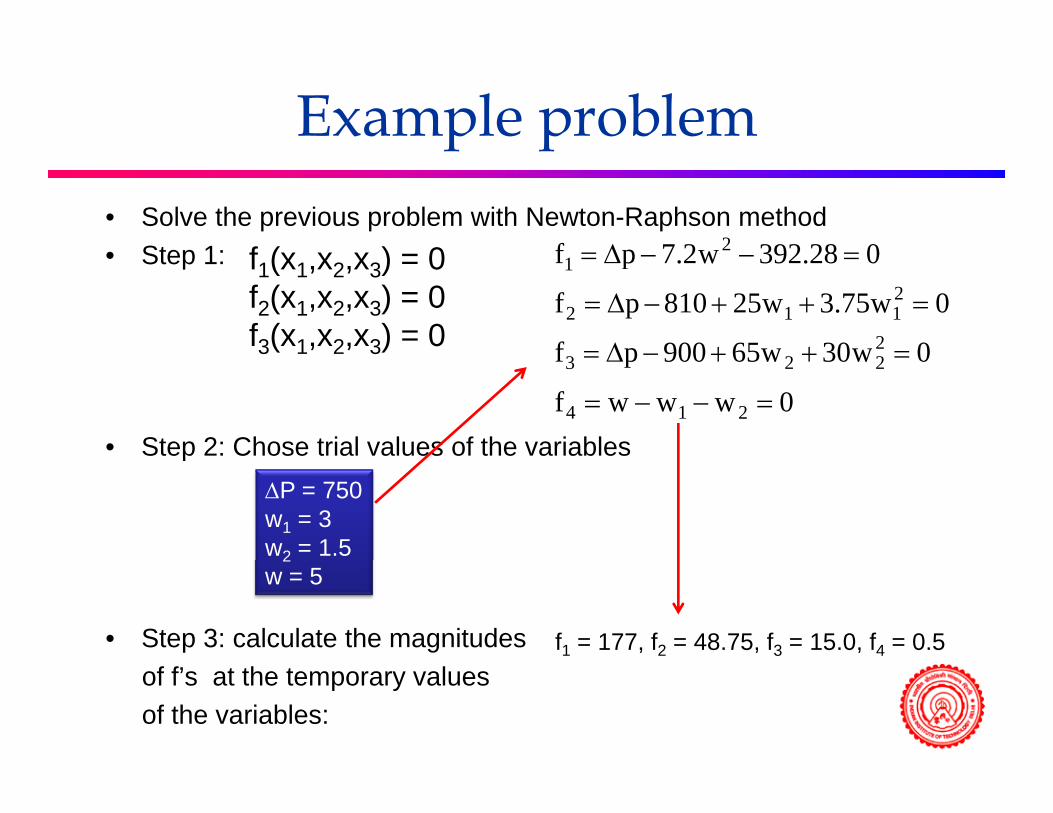
Example problem p p• Solve the previous problem with Newton-Raphson method• Step 1: 028392w27pf 2 =Δ=f (x x x ) 0• Step 1:

0w30w65900pf

0w75.3w25810pf

028.392w2.7pf

2

2112

1

=++−Δ=

=++−Δ=

=−−Δ=f1(x1,x2,x3) = 0 f2(x1,x2,x3) = 0 f3(x1,x2,x3) = 0

• Step 2: Chose trial values of the variables

0wwwf

0w30w65900pf

214

223

=−−=

=++Δ=

pΔP = 750w1 = 3w2 = 1.5

• Step 3: calculate the magnitudes

2w = 5

f1 = 177, f2 = 48.75, f3 = 15.0, f4 = 0.5of f’s at the temporary values of the variables:

Example problem p p

• Find the partial derivatives:Find the partial derivatives:• Insert Table 6.4

0w75.3w25810pf

028.392w2.7pf2112

21

=++−Δ=

=−−Δ=

∂∂∂∂

∂∂

∂∂

Δ∂∂

ffwf

wf

wf

)p(f 1

2

1

1

11

0wwwf

0w30w65900pf

p

214

2223

112

=−−=

=++−Δ=

−−−−−−∂

−−−−∂∂

Δ∂∂

fwf

)p(f

31

22 214

⎥⎤

⎢⎡ −

00547172001

−−−−−−Δ∂∂Δ∂

)p(f

)p(4

⎥⎥⎥⎥

⎦⎢⎢⎢⎢

⎣ −− 1110015501005.471

⎦⎣

Example problem p p

• Substitute the temporary values of the variables into the p yequations for the partial derivatives. Forms a set of linear simultaneous equations

⎤⎡⎤⎡Δ⎤⎡

⎥⎥⎥⎤

⎢⎢⎢⎡

=⎥⎥⎥⎤

⎢⎢⎢⎡

ΔΔΔ

⎥⎥⎥⎤

⎢⎢⎢⎡ −

1575.487.177

xxx

015501005.47172001

2

1

• Where Δxi = xi t – xi c

⎥⎥

⎦⎢⎢

⎣⎥⎥

⎦⎢⎢

⎣ΔΔ

⎥⎥

⎦⎢⎢

⎣ −− 5.015

xx

1110015501

4

3

i i,t i,c

• Solution of simultaneous equationsΔx1 = 98.84, Δx2 = -1.055, Δx3 = -0.541, Δx4 = -1.096

• The corrected value of the variables are ΔP = 750 – 98.84 = 651.16, w1 = 4.055, w2 = 2.041, w = 6.096

Example problem p p

• These variables are returned to step 3 forThese variables are returned to step 3 for the next iteration.

• The calculations converged satisfactorily• The calculations converged satisfactorily after three iterationsT bl 6 5• Table 6.5

Simulation of a Gas Turbine System

Optimizationp

MEL 806Thermal System Simulation (2-0-2)

Dr. Prabal TalukdarAssociate Professor

Department of Mechanical EngineeringIIT DelhiIIT Delhi

Introduction

• In the preceding lectures, we focused our attention on obtaining a workable, feasible, or acceptable design of a system. Such a design satisfies the requirements for the given application, without violating any imposed constraints. A system fabricated or assembled b f thi d i i t d t f th i t t kbecause of this design is expected to perform the appropriate tasks for which the effort was undertaken.

• However, the design would generally not be the best design, where th d fi iti f b t i b d t f ffi ithe definition of best is based on cost, performance, efficiency or some other such measure.

• In actual practice, we are usually interested in obtaining the best lit f it t ith t bl i t lquality or performance per unit cost, with acceptable environmental

effects. This brings in the concept of optimization, which minimizes or maximizes quantities and characteristics of particular interest to a given applicationgiven application.

Examplep

• Optimization is by no means a new concept. In our daily lives, we attempt to optimize by seeking to obtain the largest amount of goods or output per unit expenditure, this being the main idea behind clearance sales and competition.

• In the academic world, most students try to achieve the best grades with the least amount of work, hopefully without violating the constraints imposed by

thi d l tiethics and regulations• The value of various items, including consumer products like

televisions, automobiles, cameras, vacation trips, advertisements, d d ti d ll t i ft t d t i di t thand even education, per dollar spent, is often quoted to indicate the

cost effectiveness of these items.

Optimization in designp g

• The need to optimize is similarly very important in design and has become particularly crucial in recent times due to growing global competition. It is no longer enough to obtain a workable system that performs the desired tasks and meets the given constraints. At the

l t l k bl d i h ld b t d d thvery least, several workable designs should be generated and the final design, which minimizes or maximizes an appropriately chosen quantity, selected from theseDiff t d t h t i ti b f ti l i t t i• Different product characteristics may be of particular interest in different applications and the most important and relevant ones may be employed for optimization. For instance, weight is particularly important in aerospace and aeronautical applications accelerationimportant in aerospace and aeronautical applications, acceleration in automobiles, energy consumption in refrigerators, and flow rate in a water pumping system. Thus, these characteristics may be chosen for minimization or maximizationfor minimization or maximization.

Workable/Optimum designp g

• Workable designs are obtained over the allowable ranges of the design variables in order t ti f th ito satisfy the given requirements and constraintsO ti i ti t i t fi d• Optimization tries to find the best solution, one that minimizes or maximizes a feature ormaximizes a feature or quantity of particular interest in the application under consideration The optimum design in a domain of under consideration p g

acceptable designs

Basic concepts of optimizationp p

Objective functionObjective function• Any optimization process requires specification of a

quantity or function that is to be minimized or maximized. This function is known as the objective function, and it represents the aspect or feature that is of particular interest in a given circumstance. g

• Though the cost, including initial and maintenance costs, and profit are the most commonly used quantities to be

ti i d th t l d foptimized, many others aspects are employed for optimization, depending on the system and the application.

Examples of Objective Functionp j

The objective functions that are optimized for thermal systems are frequently j p y q ybased on the following characteristics: 1. Weight2. Size or volume3 Rate of energy consumption3. Rate of energy consumption4. Heat transfer rate5. Efficiency6. Overall profit7. Costs incurred8. Environmental effects9. Pressure head needed10 Durability and dependability10. Durability and dependability11. Safety12. System performance13. Output delivered14. Product quality

Let us denote the objective functionLet us denote the objective function that is to be optimized by U, where U is a function of the n independent variables in the problem x1, x2, x3, . . . p 1, 2, 3,, xn. Then the objective function and the optimization process may be expressed asU = U (x1, x2, x3, . . . , xn) → Uoptwhere Uopt denotes the optimal value of U. The x’s represent the design

i bl ll h ivariables as well as the operating conditions, which may be changed to obtain a workable or optimal design

Global maximum of the objective functionGlobal maximum of the objective function U in an acceptable design domainof the design variable x1.

Constraints

• The constraints in a given design problem arise due to limitations on the ranges of the physical variables, and due to the basic conservation principles that must be satisfied.

• The restrictions on the variables may ariseThe restrictions on the variables may arise due to the space, equipment, and materials being employed. These may restrict the dimensions of the system, the highest y gtemperature that the components can safely attain, allowable pressure, material flow rate, force generated, and so on. Minimum values of the temperature may be specified for thermoforming of a plastic and for ignition to occur in an engine. Th s both minim m and ma im m al es• Thus, both minimum and maximum values of the design variables may be involved

Equality Constraintsq y

• Many constraints arise because of the conservation laws, particularly those related to mass, momentum, and energy in thermal systems.

• Thus, under steady-state conditions, the mass inflow into the system must equal the mass outflow. This condition gives rise to an equation that must be satisfied by the relevant design variables, thus restricting the values that may be employed in the search for an

tioptimum.• There are two types of constraints, equality constraints and

inequality constraints. As the name suggests, equality constraints ti th t b ittare equations that may be written as

Inequality Constraintsq y

• Similarly, inequality constraints indicate the maximum or minimum value of a function and may be written as

• The m equality and n equality constraints are given for a general ti i ti bl i t f th f ti G d H hi hoptimization problem in terms of the functions G and H, which are

dependent on the n design variables x1, x2, ----- , xn.

Examplep

• The equality constraints are most commonly obtained from conservation laws; e.g., for a steady flow circumstance in a control volume, we may write

or

• It is generally easier to deal with equations than with inequalities because many methods are available to solve different types of

ti d t f ti h h hequations and systems of equations whereas no such schemes are available for inequalities

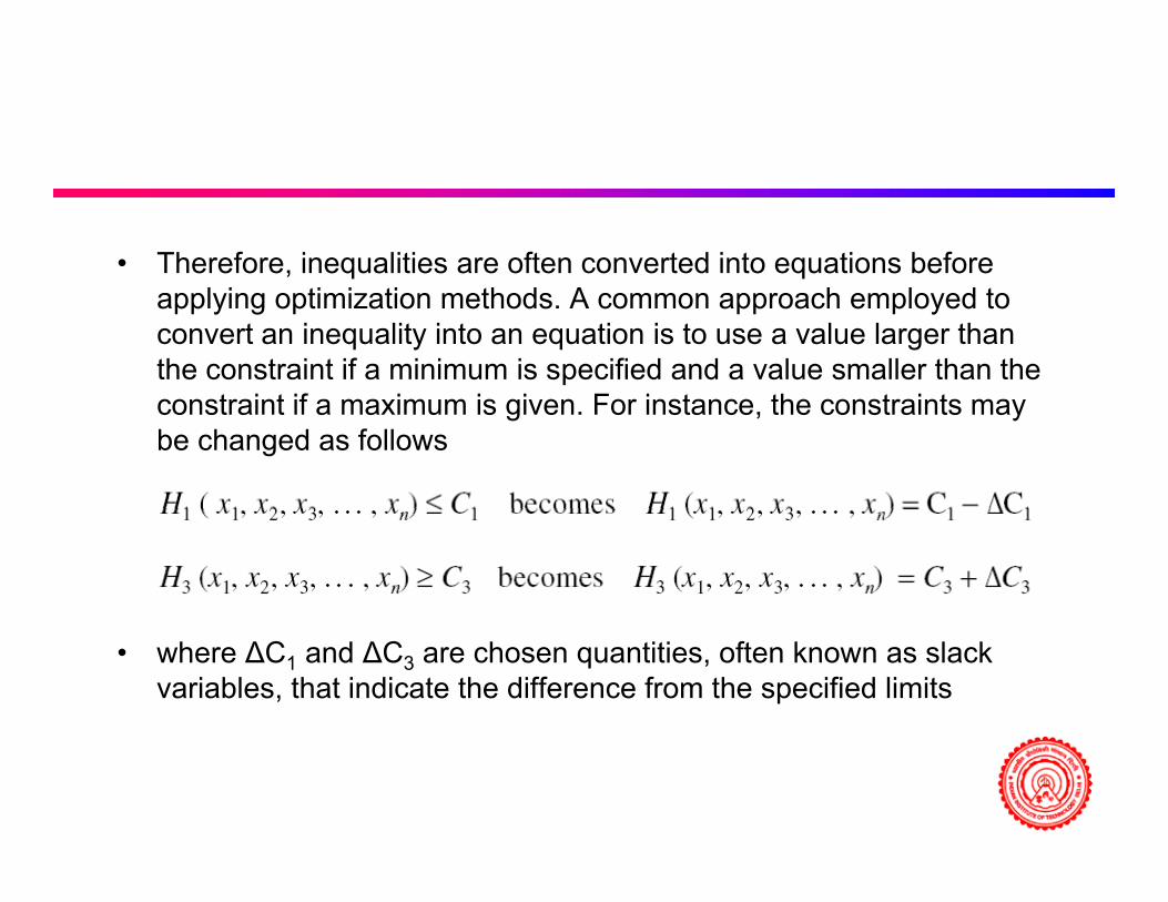
• Therefore, inequalities are often converted into equations before applying optimization methods. A common approach employed to convert an inequality into an equation is to use a value larger than the constraint if a minimum is specified and a value smaller than the

t i t if i i i F i t th t i tconstraint if a maximum is given. For instance, the constraints may be changed as follows

• where ∆C1 and ∆C3 are chosen quantities, often known as slack variables, that indicate the difference from the specified limits

Mathematical Formulation

The various steps involved in the formulation of the problem are1. Determination of the design variables, xi where i = 1, 2, 3, . . . , n2. Selection and definition of the objective function, U3 Determination of the equality constraints Gi = 0 where i = 1 2 33. Determination of the equality constraints, Gi = 0, where i = 1, 2, 3,

... , m4. Determination of the inequality constraints, Hi ≤ or ≥ Ci, where i = 1,

2 3 l2, 3, . .l5. Conversion of inequality constraints to equality constraints, if

appropriate

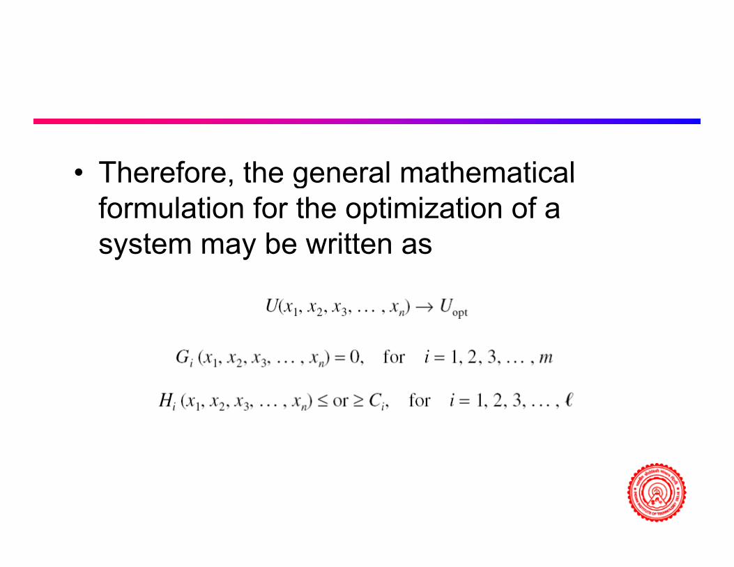
• Therefore the general mathematicalTherefore, the general mathematical formulation for the optimization of a system may be written assystem may be written as

• If the number of equality constraints m is equal to the q y qnumber of independent variables n, the constraint equations may simply be solved to obtain the variables and there is no optimization problemand there is no optimization problem.

• If m > n, the problem is overconstrained and a unique solution is not possible because some constraints have to be discarded to obtain a solution.

• If m < n, an optimization problem is obtained. Th i lit t i t ll l d t• The inequality constraints are generally employed to define the range of variation of the design parameters

Optimization methodsp• There are several methods that may be employed for solving

the mathematical problem to optimize a system or a processthe mathematical problem to optimize a system or a process. • Each approach has its limitations and advantages over the

others. Thus, for a given optimization problem, a method may b ti l l i t hil f th th tbe particularly appropriate while some of the others may not even be applicable.

• The choice of method largely depends on the nature of the equations representing the objective function and the constraints.

• Because of the complicated nature of typical thermal systems,Because of the complicated nature of typical thermal systems, numerical solutions of the governing equations and experimental results are often needed to study the behavior of the objective function as the design variables are varied andthe objective function as the design variables are varied and to monitor the constraints.

• However, in several cases, detailed numerical results , ,are generated from a mathematical model of the system or experimental data are obtained from a physical model, and these are curve fitted to obtain algebraic equationsand these are curve fitted to obtain algebraic equations to represent the characteristics of the system.

• Optimization of the system may then be undertaken based on these relatively simple algebraic expressions and equations

Calculus methods

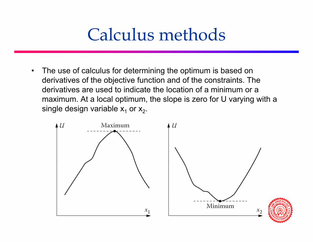
• The use of calculus for determining the optimum is based on derivatives of the objective function and of the constraints. The derivatives are used to indicate the location of a minimum or a maximum. At a local optimum, the slope is zero for U varying with a i l d i i blsingle design variable x1 or x2.

Lagrange multipliersg g p

• An important method that employs calculus for optimization is the method of Lagrange multipliers.

• The objective function and the constraints are combined through the use of constants known as Lagrange multipliers, to yield a system of algebraic equations.

• These equations are then solved analytically or numerically to obtain the optimum as well as the values of the multipliers.

• However, curve fitting often requires extensive data that may involve detailed experimental measurements or numerical simulations of the psystem. Since this may demand a considerable amount of effort and time, particularly for thermal systems, it is generally preferable to use other methods of optimization that require relatively smaller numbers of simulations.

Examplep

• From StoeckerFrom Stoecker

Search Methods

• In the simplest approach, the objective function is calculated at uniformly spaced locations in the domain, selecting the design with the optimum value. This approach, known as exhaustive search, is not very imaginative and is clearly an inefficient method to optimize

ta system• Because of the effort involved in experimentally or numerically

simulating typical thermal systems, particularly large and complex t it i i t t t i i i th b f i l tisystems, it is important to minimize the number of simulation runs or

iterations needed to obtain the optimum• Search methods such as dichotomous, Fibonacci, univariate, and

t t t t t ith i iti l d i d tt t tsteepest ascent start with an initial design and attempt to use a minimum number of iterations to reach close to the optimum

• The exact optimum is generally not obtainedThe exact optimum is generally not obtained even for continuous functions because only a finite number of iterations are used. However, in actual engineering practice, components, materials, and even dimensions are not

il bl ti titi b tavailable as continuous quantities but as discrete steps.

• For instance a heat exchanger would typically• For instance, a heat exchanger would typically be available for discrete heat transfer rates such as 50 100 200 kW etcas 50, 100, 200 kW, etc

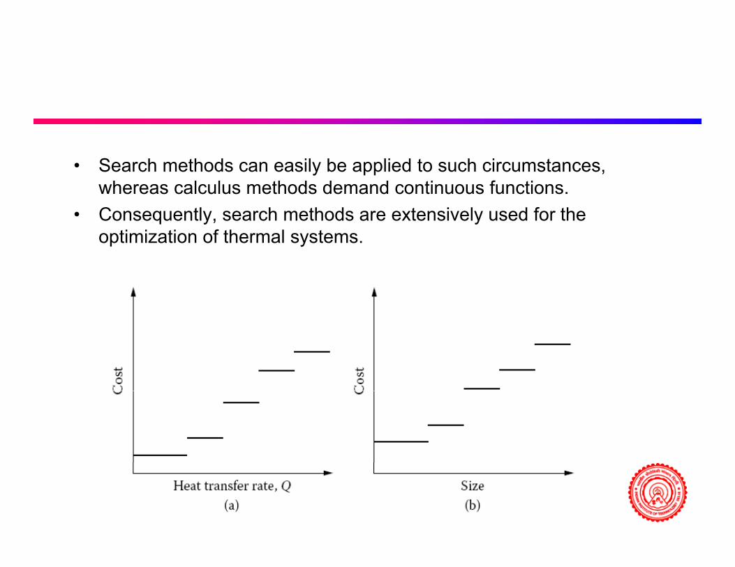
• Search methods can easily be applied to such circumstances, whereas calculus methods demand continuous functions.

• Consequently, search methods are extensively used for the optimization of thermal systems.

Linear and Dynamic Programming

• Linear programming is an important optimization method p g g p pand is extensively used in industrial engineering, operations research, and many other disciplines. H th h b li d l if th• However, the approach can be applied only if the objective function and the constraints are all linear.

• Large systems of variables can be handled by thisLarge systems of variables can be handled by this method, such as those encountered in air traffic control, transportation networks, and supply and utilization of raw materialsmaterials.

• However, thermal systems are typically represented by nonlinear equations.q

Dynamic Programmingy g g

• Dynamic programming is used to obtain the best path through a series of stages or steps to achieve a given task, for instance, the optimum configuration of a manufacturing line, the best path for the flow of hot water in a building, and the best layout for transport of

l i l tcoal in a power plant.

Dynamic Programmingy g g

• Therefore, the result obtained from dynamic , yprogramming is not a point where the objective function is optimum but a curve or path over which the function is optimizedoptimized.

• The optimum path is the one over which a given objective function, say, total transportation cost, is minimized.

• Though unique optimal solutions are generally obtained in practical systems multiple solutions are possible andin practical systems, multiple solutions are possible and additional considerations, such as safety, convenience, availability of items, etc., are used to choose the best design

Geometric Programmingg g• Geometric programming is an optimization method that can be

applied if the objective function and the constraints can be written asapplied if the objective function and the constraints can be written as sums of polynomials. The independent variables in these polynomials may be raised to positive or negative, integer or noninteger exponents, e.g.,

• Curve fitting of experimental data and numerical results for thermal systems often leads to polynomials and power-law variations.

• Therefore, geometric programming is particularly useful for theTherefore, geometric programming is particularly useful for the optimization of thermal systems if the function to be optimized and the constraints can be represented as sums of polynomials

• However, unless extensive data and numerical simulation results o e e , u ess e te s e data a d u e ca s u at o esu tsare available for curve fitting, and unless the required polynomial representations are obtained, the geometric programming method cannot be used for common thermal systems.

• Alternative: search methods

Other Optimization Methodsp

• Among the methods that may beAmong the methods that may be mentioned are genetic algorithms (GAs), artificial neural networks (ANNs) fuzzyartificial neural networks (ANNs), fuzzy logic, and response surfaces.

Optimizationp

MEL 806Thermal System Simulation (2-0-2)

Dr. Prabal TalukdarAssociate Professor

Department of Mechanical EngineeringIIT DelhiIIT Delhi

Introduction

• In the preceding lectures, we focused our attention on obtaining a workable, feasible, or acceptable design of a system. Such a design satisfies the requirements for the given application, without violating any imposed constraints. A system fabricated or assembled b f thi d i i t d t f th i t t kbecause of this design is expected to perform the appropriate tasks for which the effort was undertaken.

• However, the design would generally not be the best design, where th d fi iti f b t i b d t f ffi ithe definition of best is based on cost, performance, efficiency or some other such measure.

• In actual practice, we are usually interested in obtaining the best lit f it t ith t bl i t lquality or performance per unit cost, with acceptable environmental

effects. This brings in the concept of optimization, which minimizes or maximizes quantities and characteristics of particular interest to a given applicationgiven application.

UNCONSTRAINED SEARCH WITH MULTIPLE VARIABLES

Let us now consider the search for an optimal design when the system is governed by two or more independent variables.

However, the complexity of the problem rises sharply as the number of variables increases andsharply as the number of variables increases and, therefore, attention is generally directed at the most important variables, usually restricting these to two p y gor three.

• In addition, many practical thermal systems canIn addition, many practical thermal systems can be well characterized in terms of two or three predominant variables.

• Examples of this include the length and diameter of a heat exchanger, fluid flow rate and evaporator temperature in a refrigeration system, and so on.

• In order to graphically depict the iterativeIn order to graphically depict the iterative approach to the optimum design, a convenient method is the use of contoursconvenient method is the use of contours or lines of constant values of the objective functionfunction.

Lattice Search Method

Lattice search method in a two-variable space.

Univariate Search

• An univariate search involves optimizing theAn univariate search involves optimizing the objective function with respect to one variable at a time. Therefore, the multivariable problem is reduced to a series of single-variable optimization problems, with the process

i t th ti th i blconverging to the optimum as the variables are alternated

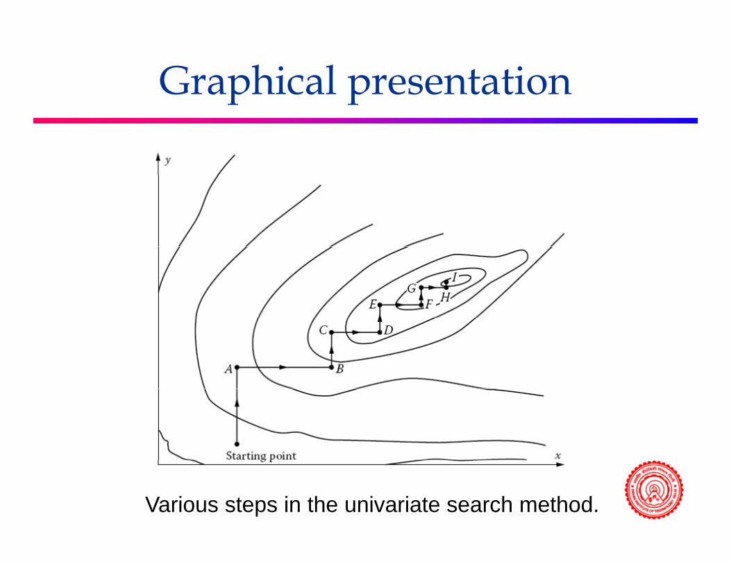
Graphical presentationp p

Various steps in the univariate search method.

The methodA starting point is chosen based on available information on the system or as a point away from the boundaries of the regionor as a point away from the boundaries of the region.

First, one of the variables, say x, is held constant and the function is optimized with respect to the other variable y.

Point A represents the optimum thus obtained. Then y is held constant at the value at point A and the function is optimized with respect to x to obtain the optimum given by point B. p g y p

Again, x is held constant at the value at point B and y is varied to obtain the optimum, given by point C.

This process is continued, alternating the variable, which is changed while keeping the others constant, until the optimum is attained.

This is indicated by the change in the objective function, from one step y g j , pto the next, becoming less than a chosen convergence criterion or tolerance

Examplep

• The objective function U, which represents the cost of a j , pfan and duct system, is given in terms of the design variables x and y, where x represents the fan capacity and y the duct length asand y the duct length, as

• Both x and y are real and positive. Using the univariate search, obtain the optimum value of U and the corresponding values of x and y. Is this optimum a minimum or a maximum?minimum or a maximum?

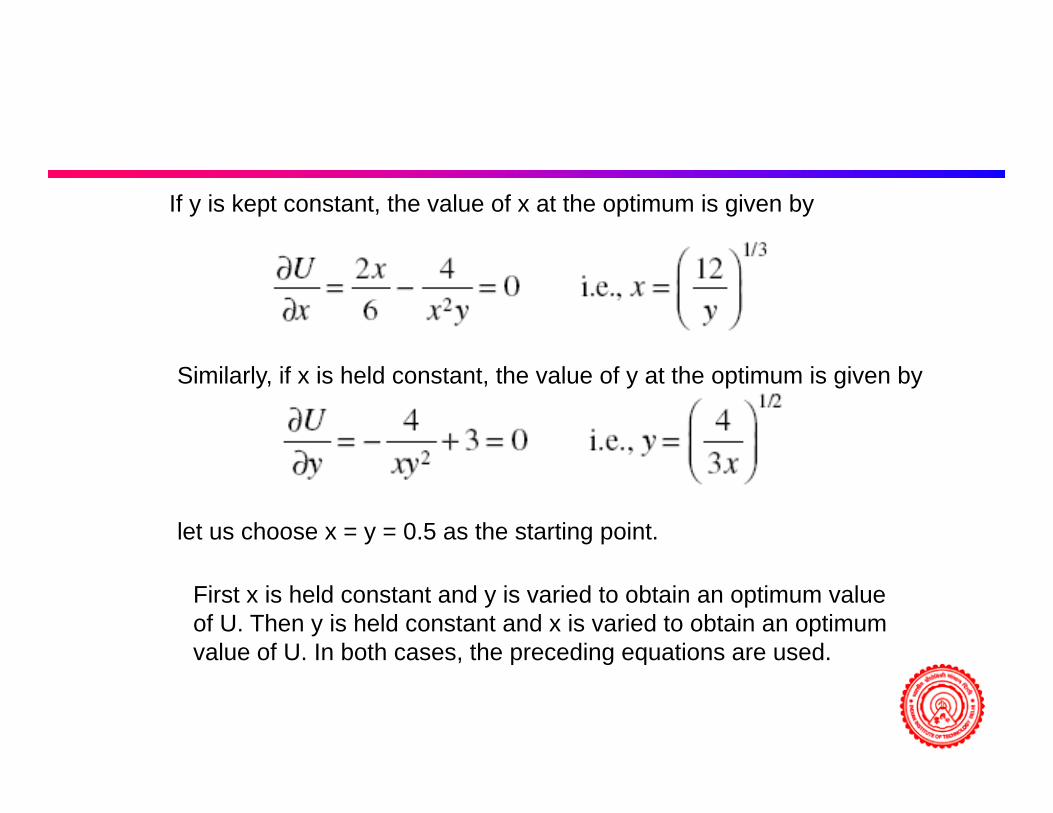
If y is kept constant, the value of x at the optimum is given by

Similarly, if x is held constant, the value of y at the optimum is given by

let us choose x = y = 0.5 as the starting point.

First x is held constant and y is varied to obtain an optimum value of U. Then y is held constant and x is varied to obtain an optimumvalue of U. In both cases, the preceding equations are used., p g q

Calculations

x y u0.5 1.632993 9.839626

1.944161 0.828139 5.5987942.437957 0.739531 5.4277912 531677 0 725714 5 4225132.531677 0.725714 5.4225132.547644 0.723436 5.4223632.550314 0.723057 5.4223592.55076 0.722994 5.4223592.550834 0.722983 5.4223592.550847 0.722982 5.4223592.550847 0.722982 5.422359

Steepest Ascent/Descent Methodp

• The steepest ascent/descent method is a very efficient p ysearch method for multivariable optimization and is widely used for a variety of applications, including thermal systemsthermal systems.

• It is a hill-climbing technique in that it attempts to move toward the peak, for maximizing the objective function, or toward the valley, for minimizing the objective function, over the shortest possible path.

• The method is termed steepest ascent in the former• The method is termed steepest ascent in the former case and steepest descent in the latter.

• At each step, starting with the initial trial point, the di ti i hi h th bj ti f ti h t thdirection in which the objective function changes at the greatest rate is chosen for moving the location of the point, which represents the design on the multivariable p p gspace.

Steepest ascent method, shown in terms of (a) the climb toward the peak of a hill and (b) in terms of constant U contours.

• It was shown that the gradient vector is normal to U∇gthe constant U contour line in a two-variable space, to the constant U surface in a three-variable space, and so onon.

• Since the normal direction represents the shortest distance between two contour lines, the direction of the gradient vector is the direction in which U changes at the greatest rate.

• For a multivariable problem the gradient vector may be

U∇

• For a multivariable problem, the gradient vector may be written as

• At each trial point, the gradient vector is determined and p , gthe search is moved along this vector, the direction being chosen so that U increases if a maximum is sought, or U decreases if a minimum is of interestdecreases if a minimum is of interest.

• The direction represented by the gradient vector is given by the relationship between the changes in the independent variables. Denoting these by Δx1, Δx2 , ---Δxn , we have

First approachpp

• Choose a starting point. Select Δx. Calculate the g pderivatives.

• Decide the direction of movement, i.e., whether Δx is iti ti C l l t Δ Obt i th lpositive or negative. Calculate Δy. Obtain the new values

of x, y, and U. • Calculate the derivatives again at this point. RepeatCalculate the derivatives again at this point. Repeat

previous steps to attain new point. • This procedure is continued until the change in the

i bl b t t ti it ti i ithivariables between two consecutive iterations is within a desired convergence criterion.

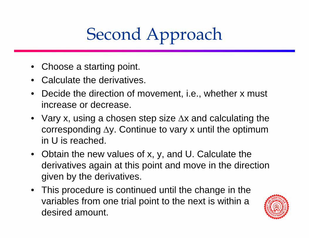
Second Approachpp

• Choose a starting point. • Calculate the derivatives. • Decide the direction of movement, i.e., whether x must

increase or decreaseincrease or decrease.• Vary x, using a chosen step size Δx and calculating the

corresponding Δy. Continue to vary x until the optimum p g y y pin U is reached.

• Obtain the new values of x, y, and U. Calculate the derivatives again at this point and move in the directionderivatives again at this point and move in the direction given by the derivatives.

• This procedure is continued until the change in the p gvariables from one trial point to the next is within a desired amount.

Example Problemp

• Consider the simple problem discussedConsider the simple problem discussed before and apply the two approaches just discussed for the steepest ascent/descentdiscussed for the steepest ascent/descent method to obtain the minimum cost U.

• The starting point is taken as x = y = 0.5. The results g p yobtained for different values of Δx are

• Therefore, if Δx1 is chosen, the changes in the other , 1 , gvariables must be calculated from these equations. In addition, Δx1 is taken as positive or negative, depending on whether U increases or decreases with x andon whether U increases or decreases with x1 and whether a maximum or a minimum is sought

Multivariable Constrained OptimizationOptimization

• We now come to the problem of constrainedWe now come to the problem of constrained optimization, which is much more involved than the various unconstrained optimization cases considered thus far.

• The number of independent variables must be larger than the number of equality constraints; otherwise, these constraints may simply be used to determine the variables and no optimization isto determine the variables and no optimization is possible

Penalty Function Methody

• The basic approach of this method is to convert the ppconstrained problem into an unconstrained one by constructing a composite function using the objective function and the constraintsfunction and the constraints

• Let us consider the optimization problem given by the equations

• The composite function, also known as the penalty function, may be formulated in many different ways.

• If a maximum in U is being sought, a new objective function V is defined asfunction V is defined as

• and if a minimum in U is desired, the new objectiveand if a minimum in U is desired, the new objective function is defined as

• Here the r’s are scalar quantities that vary the importance given to the various constraints and are known as penalty parametersknown as penalty parameters.

• They may all be taken as equal or different. • Higher values may be taken for the constraints that are

critical and smaller values for those that are not as important.

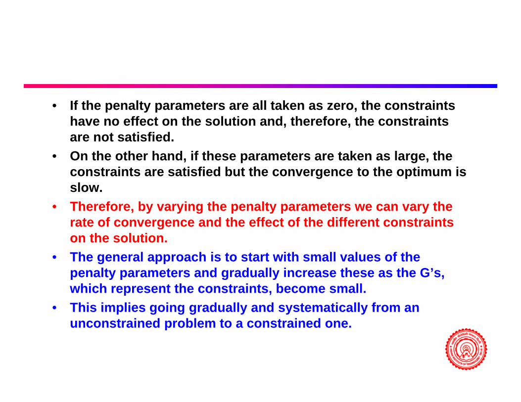
• If the penalty parameters are all taken as zero, the constraints have no effect on the solution and, therefore, the constraintshave no effect on the solution and, therefore, the constraints are not satisfied.

• On the other hand, if these parameters are taken as large, the constraints are satisfied but the convergence to the optimum isconstraints are satisfied but the convergence to the optimum is slow.

• Therefore, by varying the penalty parameters we can vary the rate of convergence and the effect of the different constraintsrate of convergence and the effect of the different constraints on the solution.

• The general approach is to start with small values of the penalty parameters and gradually increase these as the G’s, pe a ty pa a ete s a d g adua y c ease t ese as t e G s,which represent the constraints, become small.

• This implies going gradually and systematically from an unconstrained problem to a constrained one.p

Penalty function method for the combined objective function V andPenalty function method for the combined objective function V and different values of the penalty parameter r.

Examplep

where U is to be minimized. The inequality constraints give the feasible domain as 2 < x < 4. Without the constraints, the optimum is at x = –3, where U is zerowhere U is zero.

• With the constraints, the minimum is at x = 2, where U = 25/12 = 2.08.

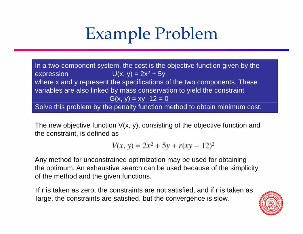
Example Problemp

In a two-component system, the cost is the objective function given by the expression U(x y) = 2x2 + 5yexpression U(x, y) = 2x2 + 5ywhere x and y represent the specifications of the two components. These variables are also linked by mass conservation to yield the constraint

G(x, y) = xy -12 = 0( y) ySolve this problem by the penalty function method to obtain minimum cost.

The new objective function V(x, y), consisting of the objective function andth t i t i d fi dthe constraint, is defined as

Any method for unconstrained optimization may be used for obtainingAny method for unconstrained optimization may be used for obtainingthe optimum. An exhaustive search can be used because of the simplicity of the method and the given functions.

If r is taken as zero the constraints are not satisfied and if r is taken asIf r is taken as zero, the constraints are not satisfied, and if r is taken as large, the constraints are satisfied, but the convergence is slow.

We may also derive x and y in terms of the penalty parameter r, by differentiating V with respect to x and y and equating the resultingdifferentiating V with respect to x and y, and equating the resulting expressions to zero, as

See the spreadsheet

Geometric Programmingg g

MEL 806Thermal System Simulation (2-0-2)

Dr. Prabal TalukdarAssociate Professor

Department of Mechanical EngineeringIIT DelhiIIT Delhi

Degree of difficultyg y

• D = N – (n + 1)D = N (n + 1)• where N is the total number of terms in the

objective function and in the constraintsobjective function and in the constraints and n is the number of independent variablesvariables

Unconstrained Optimizationp

• Single Independent VariableSingle Independent Variable

Examplep

Multiple Independent Variablesp p

Two other equations for w1 and w2 are o ot e equat o s o 1 a d 2 a eobtained from Equation by equating the sum of the exponents of each variable to zero in order to eliminate these variables from the optimum value of U.

Mathematical Proof

Objective function

The location of the optimum is found by differentiating this equation and setting the derivative equal to zeroderivative equal to zero

Multiplying by x:

withDefine a function

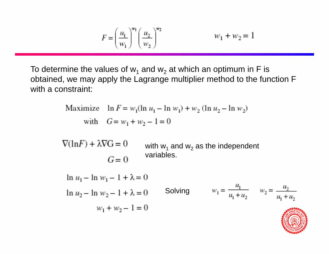
To determine the values of w1 and w2 at which an optimum in F is obtained we may apply the Lagrange multiplier method to the function Fobtained, we may apply the Lagrange multiplier method to the function F with a constraint:

i h d h i d dwith w1 and w2 as the independent variables.

Solving

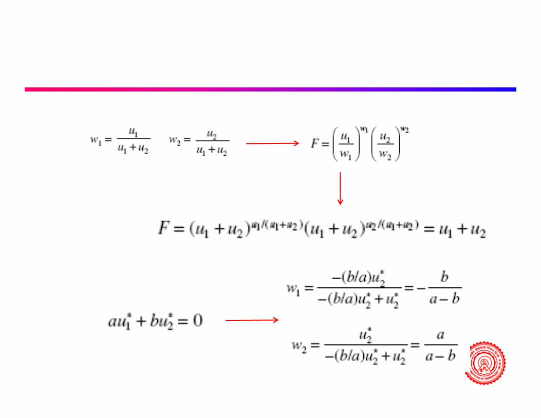
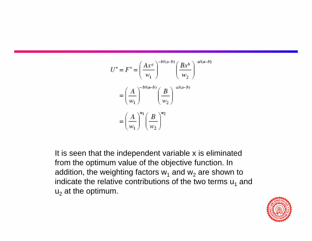
It is seen that the independent variable x is eliminated from the optimum value of the objective function. In p jaddition, the weighting factors w1 and w2 are shown to indicate the relative contributions of the two terms u1 and u2 at the optimum.

Constrained OptimizationpFive terms and four variables (x1, x2, x3, x4)

Objective function: U = u1 + u2 + u3With constraint: u4 + u5 = 1With constraint: u4 u5 1

Geometric programming gives:

With

And

with

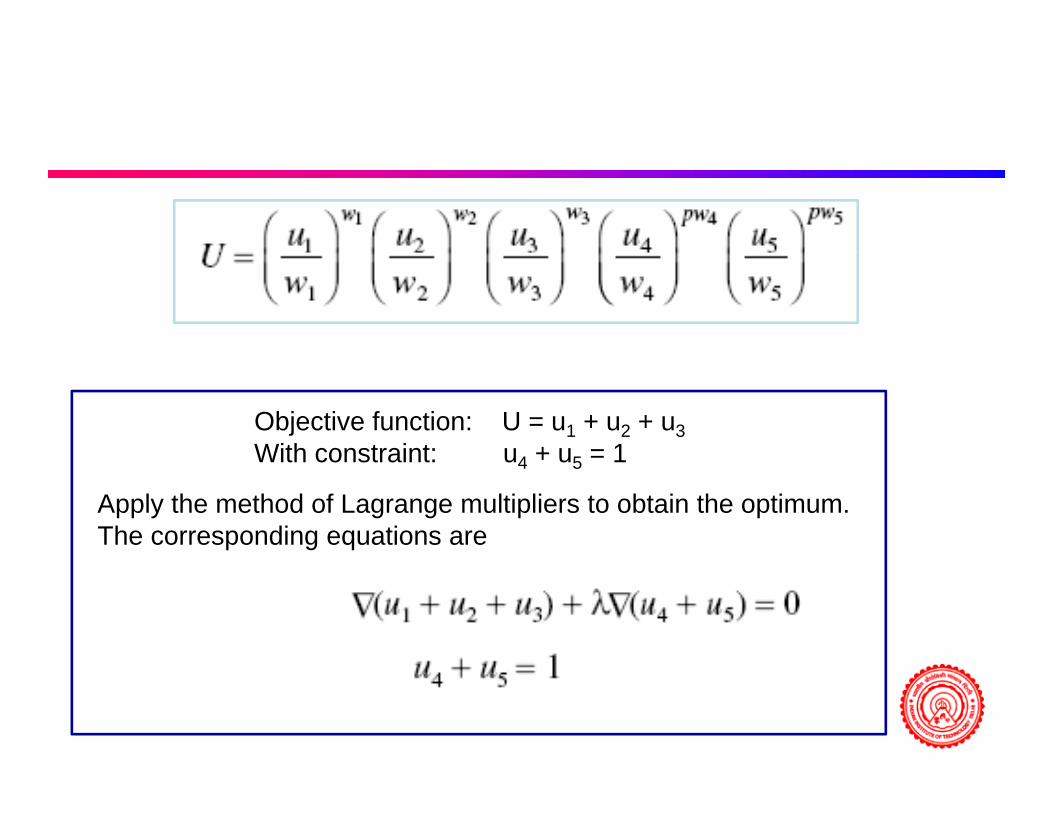
Objective function: U = u1 + u2 + u3With constraint: u4 + u5 = 1

Apply the method of Lagrange multipliers to obtain the optimum.The corresponding equations are

With constraint: u4 + u5 1

The derivatives are taken with respect to the independent variables xi, one at a time, and the resulting equations multiplied by xi.one at a time, and the resulting equations multiplied by xi.

Since p was taken as arbitrary it canas arbitrary, it can be assumed to be λ/U* in writing this equation

with

These linear equations may be solved for w1, w2, w3, w4, w5, and p.

Problem

• In a hot-rolling process, the cost C of the system is a function of the dimensionless temperature T, the thickness ratio x, and the velocity ratio y, before and after the rolls, and is given by the expression

subject to the constraints due to mass and energy balance given, respectively, as

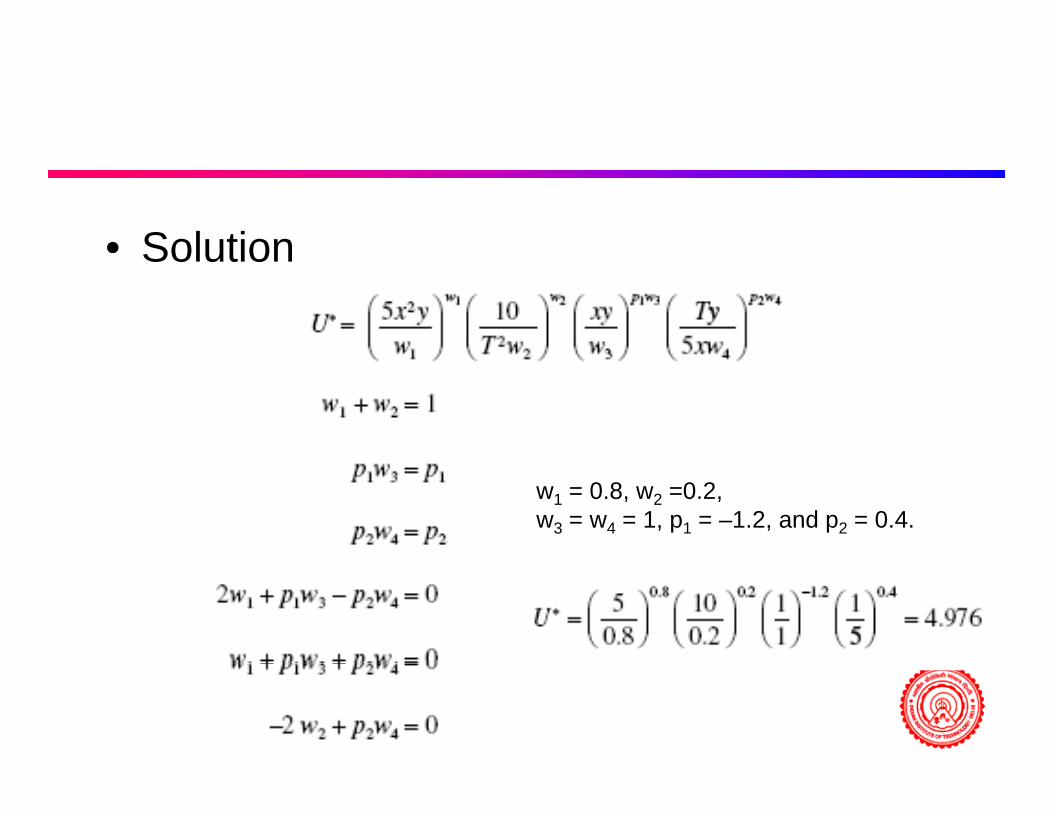
• SolutionSolution

w1 = 0.8, w2 =0.2,w3 = w4 = 1, p1 = –1.2, and p2 = 0.4.

Linear Programmingg g

• This method is applicable if the objectiveThis method is applicable if the objective functions as well as the constraints are linear functions of the independentlinear functions of the independent variables.Objective function

Subject to the constraint

• There are n variables and m linearThere are n variables and m linear equations and/or inequalities that involve these variablesthese variables.

• In linear programming, because of inequality constraints n may be greaterinequality constraints, n may be greater than, equal to, or smaller than m, unlike the method of Lagrange multipliers whichthe method of Lagrange multipliers, which is applicable only for equality constraints and for n larger than mand for n larger than m

Problem

Slack Variable

4x + 3y + s1 = 16 s1 > 0

y - 2x - s2 = -4 s2 > 0

To find the optimum value of U, two variables, in turn, are set equal to zero and the remaining variables are obtained from aequal to zero and the remaining variables are obtained from a solution of the two equations. For this problem, there are six such combinations, this number b i i l / ( )being in general [n!]/[m!(n – m)!]. The optimum is the extremum obtained from these combinations

Problem

• A company produces x quantity of one product and y of p y p q y p yanother, with the profit on the two items being four and three units, respectively. Item 1 requires one hour of facility A and three hours of facility B for fabricationfacility A and three hours of facility B for fabrication, whereas item 2 requires three hours of facility A and two hours of facility B, as shown schematically in Figure. The

f ftotal number of hours per week available for the two facilities is 200 and 300, respectively. Formulate the optimization problem and solve it by linear programming p p y p g gto obtain the allocation between the two items for maximum profit.

If s1 or s2 is negative, the solution is not allowed, since these were assumed to be

iti t ti f th t i t

Objective functionU = 4x + 3y

positive to satisfy the constraints

U 4x 3yWith constraintx + 3y ≤ 2003x + 2y ≤ 3003x + 2y ≤ 300

Introducing slack variablesx + 3y +s1 = 2003x + 2y + s2= 3003x 2y s2 300

Graphical Representationp p