Simulation of Welding Distortions in Ship Section Department of Naval Architecture And Offshore Engineering Technical University of Denmark Martin Birk-Sørensen, EF 611 Industrial PhD thesis, ATV Odense Steel Shipyard Ltd. April 1999

Welcome message from author
This document is posted to help you gain knowledge. Please leave a comment to let me know what you think about it! Share it to your friends and learn new things together.
Transcript
Simulation of WeldingDistortions in Ship Section
Department of
Naval Architecture
And Offshore Engineering
Technical University of Denmark
Martin Birk-Sørensen, EF 611Industrial PhD thesis, ATVOdense Steel Shipyard Ltd.April 1999

Simulation of WeldingDistortions in Ship Section
by
Martin Birk-SørensenDepartment of Naval Architecture
and Offshore EngineeringTechnical University of Denmark
April 1999

Copyright © 1999 Martin Birk-SørensenDepartment of Naval Architectureand Offshore EngineeringTechnical University of DenmarkDK-2800 Lyngby, DenmarkISBN 87-89502-13-2
Preface
This thesis is submitted as a partial ful�lment of the requirements for the Danish Ph.D.degree (Doctor of Philosophy). The work has been performed in collaboration with theDepartment of Naval Architecture and O�shore Engineering (ISH), the Technical Universityof Denmark, and Odense Steel Shipyard Ltd. during the period of February 1996 to January1999. Professor Dr.techn. J�rgen Juncher Jensen, ISH, and Manager Carl Erik Skj�lstrupand Dr. Henning Kierkegaard, both Odense Steel Shipyard, supervised the study.
The study was �nancially supported by the Danish Academy of Science (ATV) and OdenseSteel Shipyard Ltd. The support is gratefully acknowledged.
During my study I was given the opportunity to stay as a research fellow at Kawasaki SteelCorporation, Mizushima Works, Japan. The stay was very encouraging and gainful. I wouldlike to thank Dr. Amano, Dr. Yoshida, Mr. Oi and the rest of the sta� at the TechnicalResearch Laboratories for their help and kindness during my stay.
Special thanks go to my colleagues at the Shipyard and the Department, friends and family,and especially to my friend and contemporary M.Sc. Tommy Pedersen for help, discussions,interest and technical support.
Thanks also to all those people I was given the opportunity to meet, to cooperate with, orjust to consult frequently for going into details about the theory or the way of practice.
Martin Birk-S�rensenOdense, May 31, 1999

ii Preface
This page is intentionally left blank.
Executive Summary
Simulations of welding distortions in ship sections are performed for the purpose of estab-lishing utility-based design principles. The long-term goal is to specify an optimal weldingprocedure, and hence, to minimise distortion due to welding. In the present study, the ther-mal and the mechanical behaviour for some welded details have been investigated. To arriveat such understanding, models for thermal loading and stresses are studied and formulated.
The welding involves multifarious physical phenomena. In this thesis, the potential useful-ness of �nite element computations and of simple analytical and parametric expressions isdemonstrated by means of several examples, commonly adopted from the assembly lines atshipyards.
Inaccuracies arise partly from thermal deformations due to cutting and welding and partlyas dimensional variations due to human factors, and this increase the production costs.With the increasing use of automatisation, as seen at Odense Steel Shipyard Ltd., andhence, higher tolerance requirements, it is attractive to quantify the thermal deformationsby mathematical models, in order to reduce the amount of rework.
The objective of the present work, has been to simulate some typical welding joints. Thisincluded establishing an arbitrary moveable heat source, veri�cation measurements of thetemperature distribution in a steel plate, measurements of distortions and stresses and �niteelement models. Knowing the in uence from the welding, both qualitative and quantitative,it is possible to simulate the mechanics of the welding process. In the present work calcu-lations were performed by a �nite element program. The simulation routines were appliedto a comparison of distortions and stresses of real models. These models are both in modelsize and full-scale size.
Infrared measurements of temperature distribution in di�erent plate thicknesses, show thatthe overall best assumption about this distribution is the one made by Rosenthal, althoughRosenthal's analysis is rather inaccurate for temperatures in or near the heat-a�ected zone.In zones where the temperature is less than half the melting point, Rosenthal's solution cangive quite accurate results.
Based on the cooling rates of a weld, formulas have been derived in order to determinewhether a heat ow for di�erent types of welding and materials parameters, can be calculatedas a two-dimensional or a three-dimensional problem.
iv Executive Summary
A simple procedure for quantitative estimations of residual stresses caused by welding hasbeen outlined based on the sectioning method.
Tensile test shows that the rolling direction of a steel plate appears not to have a signi�cantin uence on the material strength.
A simple beam theory is used in order to illustrate the variation of residual stresses andcurvature on a quantitative basis.
To gain empirical knowledge of the distortions due to welding and to obtain veri�cationdata for the computer simulations, measurements are carried out on some modules in theproduction line and on test specimens in the welding laboratory. The experimental valuesare compared with parametric expressions found in the literature, and the accordance isfairly good.
In order to make a rational analysis of the stresses and distortions in ship sections causedby welding, �nite-element simulations are carried out. Simulations which involve non-linearmaterials parameters and a thermoelastic-plastic material behaviour law are complied with.
The purpose of the simulation or calculation is to obtain values for in-plane shrinkage andout-of-plane distortion. For the in-plane calculation a plane element model of a plate assum-ing a plane stress �eld works quite well. The heat source can be moved in straight lines allover the plate, by use of the developed simpli�ed Fortran subroutine. The FEM results arehere in general lower than those experimentally measured. The distortion patterns are fair.
A plane strain model of the cross-section of the symmetric T-pro�le is easy to handle andCPU e�cient. The results of this kind of analysis show high accuracy.
The moving heat source applied along the centre line of a FEM modelled two-dimensionalplate shows the same tendency in shrinkage as seen in the welding experiments.
A three-dimensional model with the moveable heat source applied are included. Thesemodels takes into account both the in-plane and out-of plane distortion. The results showno satisfying accuracy. The thermoelastic-plastic problem was to ambitious to solve for realscale models, so the achievements in a short-term view are limited and can at this level onlybe used as a leaning.
Computational welding simulations (and mechanics) are not fully established as a sciencebut almost su�ciently developed to be applied to various simpli�ed problems in the shipyardindustry.
The study has shown the advantage of using the FEM for a welding simulation tool, fortwo-dimensional models which can be used as benchmarks.

Synopsis
Simulering af svejsedeformationer i skibssektioner er unders�gt med det form�al at opstillepraktiske designregler for svejsekrymp. Det langsigtede m�al med projektet er at kunnespeci�cere en optimal svejseprocedure for derved at kunne minimere deformationer opst�aetp�a grund af svejsning. For at komme til en forst�aelse af det thermo-mekaniske problem ermodeller for termisk last og sp�nding blevet unders�gt b�ade analytisk, numerisk og eksper-imentielt.
Svejsning involverer mange fysiske f�nomener. I denne afhandling er muligheden for bereg-ning af svejsedeformationer vha. endelige elementers metode (FEM) og simple analytiske ogparametriske udtryk, demonstreret ved hj�lp af eksempler fra produktionen p�a et skibsv�rft.
De un�jagtigheder, som opst�ar under samlingen af sektioner til et skib, skyldes dels varmede-formationer som f�lge af sk�ring og svejsning og dels dimensionelle variationer grundet men-neskelige fejl, og disse f�rer til ekstra produktionsomkostninger. Med den stigende automa-tisering, som det er tilf�ldet p�a Odense Staalskibsv�rft A/S, og dermed �nere tolerancekrav,er det �nskeligt at bestemme de termiske deformationer ud fra matematiske modeller, forderved at blive i stand til at mindske det l�n-tunge opretningsarbejde.
Form�alet med n�rv�rende arbejde har v�ret at simulere nogle typiske svejste samlinger.Dette har inkluderet udviklingen af en vilk�arlig bev�gelig varmekilde, termo-mekaniske FEMmodeller, veri�kation af varmefordelingen i en st�alplade og m�alinger af deformationer ogt�jninger.
N�ar den termiske ind ydelse fra svejsningen er kendt, b�ade kvalitativt og kvantitativt, er detmuligt at simulere mekanikken i en svejseproces. I det aktuelle arbejde er beregninger udf�rtmed et kommercielt FEM program. Simuleringerne er sammenlignet med deformationer ogsp�ndinger m�alt p�a relevante samlinger. Disse modeller er b�ade udf�rt i modelst�rrelse ogi fuld-skala-st�rrelse.
Infrar�de m�alinger, optaget under svejsningen, af temperaturfordelingen i st�alplader af forskel-lig tykkelse viser, at Rosenthal's analyse af temperaturfordelingen omkring en bev�geligvarmekilde er en god antagelse, sk�nt denne analyse er un�jagtig for temperatur bestem-melse i og omkring det varmep�avirkede omr�ade. I omr�ader, hvor temperaturen er lavere endhalvdelen af smeltetemperaturen, giver Rosenthal's l�sning anvendelige resultater.

vi Synopsis
Baseret p�a afk�lingshastigheden af en svejsning, er der udledt formler til bestemmelse af, omvarmeudbredelsen som resultat af svejsemetode og materialeparametre, kan beregnes som etto-dimensionalt eller tre-dimensionalt problem.
Kvantitativ bestemmelse af svejseresidualsp�ndinger er udf�rt baseret p�a opsk�ringsmeto-den. Dette arbejde er udf�rt p�a Kawasaki Steel Corporation i Mizishima, Japan. For atunders�ge om valseretningen af st�alplader har betydning for styrkeegenskaberne, er tr�k-pr�vefors�g blevet udf�rt. Disse viser, at der ikke er en signi�kant forskel p�a styrkeegensk-aberne som funktion af valseretningen.
En simpel analytisk beregning vha. bj�lketeori er benyttet for p�a kvantitativ vis at illustrereresidual sp�ndingernes og krumningens variation med opvarmningen og den efterf�lgendeafk�ling.
For at opn�a empirisk viden om deformationer for�arsaget af svejsning og for at f�a resultatertil veri�cering af numeriske beregninger, er der udf�rt m�alinger p�a delemner i skibsv�rft-produktionen og p�a pr�veemner i svejselaboratoriet. De eksperimentielt opn�aede krympe-og deformationsv�rdier er sammenlignet med parametriske udtryk fundet i litteraturen, ogoverensstemmelsen er af varierende kvalitet.
For at kunne lave en rationel analyse af sp�ndinger og deformationer i skibssektioner for�ar-saget af svejsninger, er der udf�rt FEM beregninger. Disse beregninger involverer ikke-line�re materialeparametre og en termoelastisk-plastisk materiale lov.
Form�alet med beregningerne er at bestemme en plades deformation, b�ade i planen og vinkel-ret p�a planen. For deformations beregninger i planen bruges en model med plane ele-menter under antagelse af plan sp�ndingstistand. Denne model bruges ved beregning afen svejses�m lagt p�a en plade. FEM resultaterne er generelt lavere end de m�alte resultater,men den overordnede deformations pro�l passer tiln�rmelsesvis. En plan t�jnings modelaf et tv�rsnit af et symmetrisk T-pro�l er analyseret. Denne to-dimensionelle beregningviser �n overensstemmelse med de m�alte deformationer. En tre-dimensionel model medbev�gelig varmekilde er ogs�a inkluderet. Resultaterne afviger v�sentligt fra de eksperimen-tielt bestemte v�rdier, og b�r p�a dette niveau kun bruges som tendensberegning.
Det termoelastisk-plastiske problem har vist sig for beregnings-tungt til at bestemme defor-mationer i aktuelle svejsninger p�a produktionsstadiet. Derfor m�a beregningsbaserede svej-sedeformationer betragtes som en ikke helt f�rdigudviklet videnskab og kun delvist brugbarved l�sning af forskellige simple problemstillinger (elementartilf�lde) i skibsv�rftindustrien.
Contents
Preface i
Executive Summary iii
Synopsis (in Danish) v
Contents vii
List of Figures xv
Symbols and Nomenclature xvii
1 Introduction 1
1.1 Overview and Background . . . . . . . . . . . . . . . . . . . . . . . . . . . . 1
1.1.1 Brief Overview . . . . . . . . . . . . . . . . . . . . . . . . . . . . . . 1
1.1.2 Welding Deformation . . . . . . . . . . . . . . . . . . . . . . . . . . . 2
1.2 Objectives and Scope of the Work . . . . . . . . . . . . . . . . . . . . . . . . 4
1.3 Structure of the Thesis . . . . . . . . . . . . . . . . . . . . . . . . . . . . . . 4
2 Welding-induced Temperature Field 7
2.1 Introduction . . . . . . . . . . . . . . . . . . . . . . . . . . . . . . . . . . . . 7
2.2 Heat Conduction . . . . . . . . . . . . . . . . . . . . . . . . . . . . . . . . . 7
2.3 Quasi-stationary Temperature Distribution . . . . . . . . . . . . . . . . . . . 9

viii Contents
2.3.1 Moving Point Source . . . . . . . . . . . . . . . . . . . . . . . . . . . 11
2.3.2 Thick Plate Solution . . . . . . . . . . . . . . . . . . . . . . . . . . . 12
2.3.3 Thin Plate Solution . . . . . . . . . . . . . . . . . . . . . . . . . . . . 13
2.3.4 Medium Thick Plate Solution . . . . . . . . . . . . . . . . . . . . . . 16
2.3.5 Other Formulas . . . . . . . . . . . . . . . . . . . . . . . . . . . . . . 17
2.4 Experimental Investigation of the Temperature Distribution . . . . . . . . . 18
2.4.1 2D or 3D Heat Flow . . . . . . . . . . . . . . . . . . . . . . . . . . . 19
2.4.2 Infrared Measurements . . . . . . . . . . . . . . . . . . . . . . . . . . 23
2.4.3 V-groove . . . . . . . . . . . . . . . . . . . . . . . . . . . . . . . . . . 23
2.4.4 Bead on Plates . . . . . . . . . . . . . . . . . . . . . . . . . . . . . . 26
2.5 Comparison . . . . . . . . . . . . . . . . . . . . . . . . . . . . . . . . . . . . 30
2.5.1 V-groove . . . . . . . . . . . . . . . . . . . . . . . . . . . . . . . . . . 30
2.5.2 9mm Plate . . . . . . . . . . . . . . . . . . . . . . . . . . . . . . . . . 31
2.5.3 22mm Plate . . . . . . . . . . . . . . . . . . . . . . . . . . . . . . . . 32
2.6 Heat Source Model . . . . . . . . . . . . . . . . . . . . . . . . . . . . . . . . 33
2.6.1 Distributed Heat Source . . . . . . . . . . . . . . . . . . . . . . . . . 33
2.7 Summary . . . . . . . . . . . . . . . . . . . . . . . . . . . . . . . . . . . . . 36
3 Welding Residual Stresses 39
3.1 Introduction . . . . . . . . . . . . . . . . . . . . . . . . . . . . . . . . . . . . 39
3.1.1 Stress Expressions . . . . . . . . . . . . . . . . . . . . . . . . . . . . 41
3.2 Measurement of Welding-induced Residual Stresses . . . . . . . . . . . . . . 42
3.2.1 Tensile Test . . . . . . . . . . . . . . . . . . . . . . . . . . . . . . . . 43
3.2.2 X-ray Readings . . . . . . . . . . . . . . . . . . . . . . . . . . . . . . 45
3.2.3 Welding Experiments . . . . . . . . . . . . . . . . . . . . . . . . . . . 46
3.2.4 Measuring Technique . . . . . . . . . . . . . . . . . . . . . . . . . . . 47
3.2.5 Results . . . . . . . . . . . . . . . . . . . . . . . . . . . . . . . . . . . 51
3.3 A Simple Plate Strip Analysis . . . . . . . . . . . . . . . . . . . . . . . . . . 55

Contents ix
4 Welding Distortion Measurements 59
4.1 Introduction . . . . . . . . . . . . . . . . . . . . . . . . . . . . . . . . . . . . 59
4.2 Analysis of the Shrinkage in Test Models . . . . . . . . . . . . . . . . . . . . 62
4.2.1 Fillets . . . . . . . . . . . . . . . . . . . . . . . . . . . . . . . . . . . 62
4.2.2 Butt Welds . . . . . . . . . . . . . . . . . . . . . . . . . . . . . . . . 66
4.2.3 Bead-on-Plate Specimen Shrinkage Test . . . . . . . . . . . . . . . . 71
4.2.4 Strain Gauge Readings . . . . . . . . . . . . . . . . . . . . . . . . . . 71
4.3 Process-related Welding Distortion . . . . . . . . . . . . . . . . . . . . . . . 74
5 Thermomechanical Analysis Using FEM 81
5.1 Introduction . . . . . . . . . . . . . . . . . . . . . . . . . . . . . . . . . . . . 81
5.2 Thermal FE Analysis . . . . . . . . . . . . . . . . . . . . . . . . . . . . . . . 82
5.3 Mechanical FE Analysis . . . . . . . . . . . . . . . . . . . . . . . . . . . . . 85
5.3.1 Equilibrium Equations . . . . . . . . . . . . . . . . . . . . . . . . . . 85
5.3.2 Constitutive Equations . . . . . . . . . . . . . . . . . . . . . . . . . . 86
5.4 Element Types . . . . . . . . . . . . . . . . . . . . . . . . . . . . . . . . . . 90
5.5 Meshing . . . . . . . . . . . . . . . . . . . . . . . . . . . . . . . . . . . . . . 90
5.6 FEM Parameter Test Studies . . . . . . . . . . . . . . . . . . . . . . . . . . 91
5.6.1 Temperature Dependency in the Thermal Part . . . . . . . . . . . . . 93
5.7 Calculations of Welded Details . . . . . . . . . . . . . . . . . . . . . . . . . . 97
5.7.1 2D Plate, Plane Stress . . . . . . . . . . . . . . . . . . . . . . . . . . 97
5.7.2 Elastoplastic Models . . . . . . . . . . . . . . . . . . . . . . . . . . . 100
5.7.3 T-pro�le, Plane Strain (2D) . . . . . . . . . . . . . . . . . . . . . . . 100
5.7.4 Web Frame . . . . . . . . . . . . . . . . . . . . . . . . . . . . . . . . 105
5.7.5 T-pro�le (3D) . . . . . . . . . . . . . . . . . . . . . . . . . . . . . . . 107
x Contents
6 Parametric Expressions and Veri�cation 115
6.1 Introduction . . . . . . . . . . . . . . . . . . . . . . . . . . . . . . . . . . . . 115
6.2 Approximate Method for Fillets . . . . . . . . . . . . . . . . . . . . . . . . . 115
7 Conclusions and Recommendations 121
7.1 Conclusion . . . . . . . . . . . . . . . . . . . . . . . . . . . . . . . . . . . . . 121
7.2 Recommendations for Future Work . . . . . . . . . . . . . . . . . . . . . . . 123
7.3 Comments . . . . . . . . . . . . . . . . . . . . . . . . . . . . . . . . . . . . . 124
7.3.1 Reduction of Welding Distortions . . . . . . . . . . . . . . . . . . . . 125
7.3.2 Control Needs . . . . . . . . . . . . . . . . . . . . . . . . . . . . . . . 126
7.3.3 Expert Systems . . . . . . . . . . . . . . . . . . . . . . . . . . . . . . 126
Bibliography 129
A Simple FEM Calculation with Strain Measurements 135
A.1 FEM-Calculations . . . . . . . . . . . . . . . . . . . . . . . . . . . . . . . . . 135
A.1.1 The Finite Element Model . . . . . . . . . . . . . . . . . . . . . . . . 135
A.1.2 Temperature Distribution . . . . . . . . . . . . . . . . . . . . . . . . 136
A.1.3 Elastic-Plastic FE-Analysis . . . . . . . . . . . . . . . . . . . . . . . 137
A.1.4 FEM-Results . . . . . . . . . . . . . . . . . . . . . . . . . . . . . . . 137
A.1.5 Comparison of Results . . . . . . . . . . . . . . . . . . . . . . . . . . 138
B An Example of a Data �le 139
B.1 Introduction . . . . . . . . . . . . . . . . . . . . . . . . . . . . . . . . . . . . 139
B.2 The SYSWORLD Data File . . . . . . . . . . . . . . . . . . . . . . . . . . . 139
List of Ph.D. Theses Available from the Department 147
List of Figures
1.1 Types of welding deformations, [35]. . . . . . . . . . . . . . . . . . . . . . . . 2
1.2 Deformation of a steel plate during and after welding. . . . . . . . . . . . . . 3
1.3 Stresses according their origin in a transverse weld in the deck of a 255,000dtw tanker, [18]. . . . . . . . . . . . . . . . . . . . . . . . . . . . . . . . . . . 3
2.1 Relative position along weld centre line. . . . . . . . . . . . . . . . . . . . . 9
2.2 The three stages in the welding time problem. . . . . . . . . . . . . . . . . . 10
2.3 Moving point source on a semi-in�nite slab, Grong [21]. . . . . . . . . . . . . 12
2.4 Three-dimensional graphical representation of Rosenthal thick plate solution(schematic). . . . . . . . . . . . . . . . . . . . . . . . . . . . . . . . . . . . 13
2.5 Moving line source in a thin sheet, Grong [21]. . . . . . . . . . . . . . . . . . 14
2.6 Graphical representation of Rosenthal thin plate solution (schematic). . . . . 16
2.7 Scheme of heat ow. a) 3D ow, b) 2D ow. . . . . . . . . . . . . . . . . . . 19
2.8 Dimensionless cooling rate as a function of the dimensionless plate thickness �g. 21
2.9 Isotherms in the welding line (y = 0) as a function of the welding speed,obtained by Rosenthal 2D equation. Due to the point in�nity the curves aretruncated at T = 2500oC. . . . . . . . . . . . . . . . . . . . . . . . . . . . . 22
2.10 Infrared image of the lower surface of a V-groove. . . . . . . . . . . . . . . . 24
2.11 Upper surface temperature lines of the V-groove. . . . . . . . . . . . . . . . 25
2.12 Lower surface temperature lines for the V-groove . . . . . . . . . . . . . . . 25
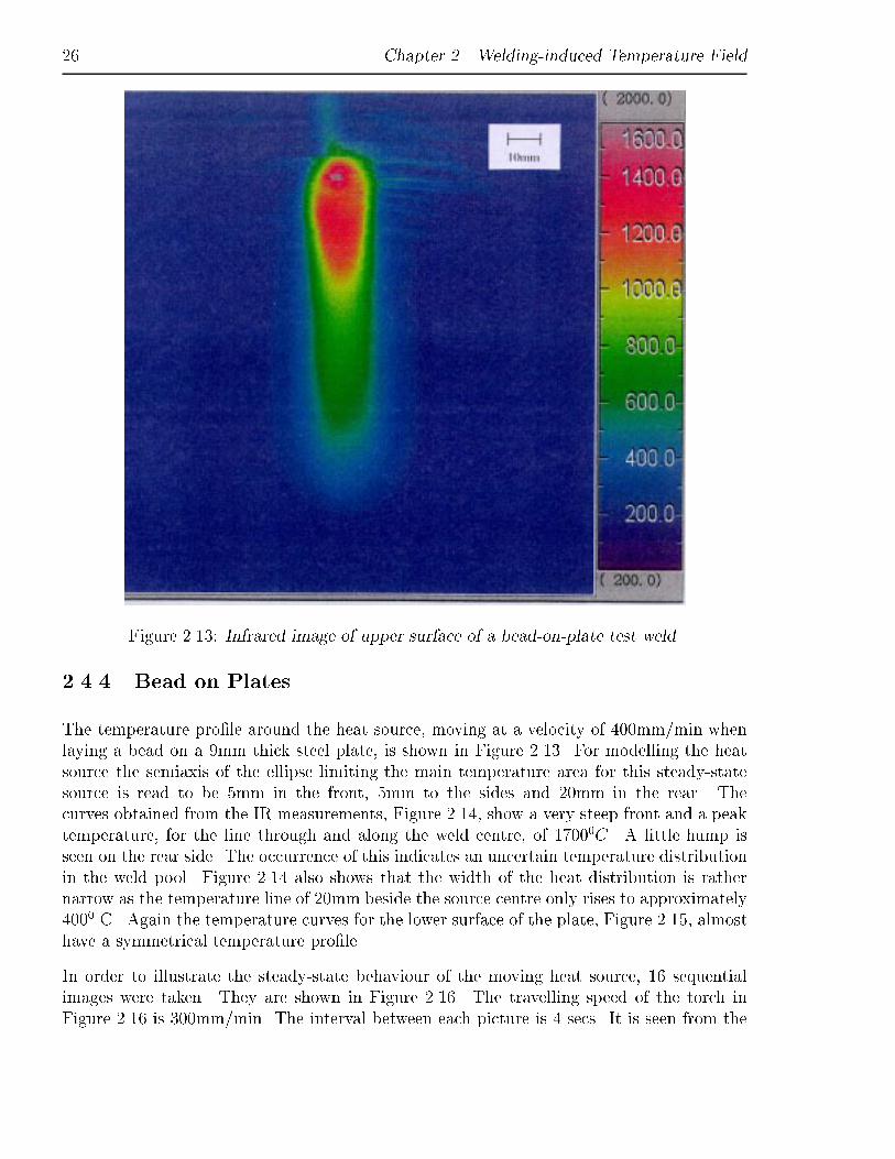
2.13 Infrared image of upper surface of a bead-on-plate test weld. . . . . . . . . . 26

xii List of Figures
2.14 Upper surface temperature lines for the 9mm plate, torch speed 400 mm/min. 27
2.15 Lower surface temperature lines for the 9 mm plate, torch speed 400 mm/min 27
2.16 16 sequential images (snapshots) for the moving heat source on the surface ofthe 9mm thick plate. . . . . . . . . . . . . . . . . . . . . . . . . . . . . . . . 28
2.17 Upper surface temperature lines of the 22mm plate, speed 300mm/min. . . . 29
2.18 Lower surface temperature lines of the 22mm plate, speed 300mm/min. . . . 29
2.19 Temperature curves along the X-axis through the centre of the heat sourcedoing the V-groove in a 22mm thick plate. . . . . . . . . . . . . . . . . . . . 30
2.20 Temperature curves along the X-axis through the centre, 9mm thick plate. . 31
2.21 Upper surface temperature curves along the X-axis 10mm beside the sourcecentre in the 9mm thick plate. . . . . . . . . . . . . . . . . . . . . . . . . . . 32
2.22 Temperature curves along the X-axis for the lower surface, 0, 10mm and 20mmbeside the source centre in the 9mm thick plate, �ltered IR measurements. . 33
2.23 Comparison of Rosenthal heat distribution equations and the measured tem-peratures on the upper surface and on the lower surface of the 22mm thickplate, �ltered IR measurements. . . . . . . . . . . . . . . . . . . . . . . . . . 34
2.24 Double ellipsoidal heat input distribution, (Wm3 ). . . . . . . . . . . . . . . . . 35
3.1 Schematic representation of changes in temperature �T and stresses duringwelding, [35]. . . . . . . . . . . . . . . . . . . . . . . . . . . . . . . . . . . . 40
3.2 Idealised stress-strain relation in the HAZ for a butt weld in a steel plate. . . 42
3.3 Di�raction resulting from re ection from adjacent atomic planes of a monochro-matic plane wave. . . . . . . . . . . . . . . . . . . . . . . . . . . . . . . . . . 46
3.4 Stress level, before welding, in a 22mm plate of three di�erent steel qualities,obtained in the present study by X-ray test. . . . . . . . . . . . . . . . . . . 47
3.5 Locations of strain gauges on the steel plate. . . . . . . . . . . . . . . . . . . 49
3.6 The 16 small sliced strain gauge pieces. . . . . . . . . . . . . . . . . . . . . . 50
3.7 Residual stresses around the weld line, SS400 steel. . . . . . . . . . . . . . . 52
3.8 Residual stresses around the weld line, low carbon steel. . . . . . . . . . . . . 52
List of Figures xiii
3.9 Residual stresses around the weld line, 9%Ni steel. . . . . . . . . . . . . . . . 53
3.10 Sectioning of the 20mm thick block into a 3mm thick block mounted with astrain gauge. . . . . . . . . . . . . . . . . . . . . . . . . . . . . . . . . . . . . 54
3.11 Biaxial calculated stress for 3mm and 20mm thick gauge cubes, low carbonsteel. . . . . . . . . . . . . . . . . . . . . . . . . . . . . . . . . . . . . . . . . 55
3.12 Stresses after heating of the upper half of the plate strip. . . . . . . . . . . . 57
3.13 Residual stresses �res after cooling. . . . . . . . . . . . . . . . . . . . . . . . 58
4.1 The �xture board, with three supports and pins for dialindicators. . . . . . . 62
4.2 A T-pro�le clamped by the �xture. . . . . . . . . . . . . . . . . . . . . . . . 62
4.3 Cross-section of the T-pro�le in the �xture, without clamp plate. . . . . . . . 63
4.4 The tool used for measuring the relatively small shrinkage values. . . . . . . 63
4.5 The strain gauge locations on the "back"side of the T-pro�le. . . . . . . . . 63
4.6 The strain gauge locations on the "front" side of the T-pro�le. . . . . . . . . 63
4.7 T-specimen with prescribed cooling boundary condition. . . . . . . . . . . . 65
4.8 Longitudinal shrinkage for the forced air-cooled T-pro�le, sample 11. . . . . 65
4.9 Longitudinal strain for butt welds with tap plates. . . . . . . . . . . . . . . . 66
4.10 Transverse strain for butt welds with tap plates. . . . . . . . . . . . . . . . . 67
4.11 Measured out-of-plane deformation for butt weld, max. angular de ection. . 68
4.12 Geometric change of a 200 x 160 x 10mm steel plate after welding of a V-groove, [34]. . . . . . . . . . . . . . . . . . . . . . . . . . . . . . . . . . . . . 70
4.13 Geometric change of a 400 x 300 x 12mm steel plate after welding of a V-grove,present measurements. . . . . . . . . . . . . . . . . . . . . . . . . . . . . . . 70
4.14 T-pro�le in bending. . . . . . . . . . . . . . . . . . . . . . . . . . . . . . . . 73
4.15 Erection of sti�ener on the web. . . . . . . . . . . . . . . . . . . . . . . . . . 74
4.16 The test specimen for out-of-plane deformation measurements. . . . . . . . . 75
4.17 The web specimen with the sti�ener, the used co-ordinate system, and thelocation of measure points. . . . . . . . . . . . . . . . . . . . . . . . . . . . . 77

xiv List of Figures
4.18 The Heat-A�ected Zone for MAG and laser welding. . . . . . . . . . . . . . 78
5.1 Structure of SYSWELD, [56]. . . . . . . . . . . . . . . . . . . . . . . . . . . 83
5.2 Isotropic strain-hardening. . . . . . . . . . . . . . . . . . . . . . . . . . . . . 89
5.3 Kinematic strain-hardening. . . . . . . . . . . . . . . . . . . . . . . . . . . . 89
5.4 Strain-hardening slope depending on both plastic strain and temperature. . . 89
5.5 The triangular mesh, the geometry and the constraints for the model of theT-pro�le. . . . . . . . . . . . . . . . . . . . . . . . . . . . . . . . . . . . . . . 92
5.6 Load cases for heating and the belonging de ection for the ange of the T-pro�le. 94
5.7 Residual de ection as a function of the yield stress. . . . . . . . . . . . . . . 96
5.8 Residual de ection as a function of the �llet size. . . . . . . . . . . . . . . . 96
5.9 Temperature-dependent materials properties for mild steel as used in the FEMcalculations. . . . . . . . . . . . . . . . . . . . . . . . . . . . . . . . . . . . . 96
5.10 Elements and temperature pro�le around a heat source moving at 7 mm/s. . 98
5.11 Temperature distribution along the top of a thick plate, perpendicular to theweld, after quasi-steady state has been reached. The welding speed approxi-mately 5mm/s. . . . . . . . . . . . . . . . . . . . . . . . . . . . . . . . . . . 99
5.12 Temperature in the plate after cooling. . . . . . . . . . . . . . . . . . . . . . 100
5.13 Deformation of the plate, legend text for longitudinal shrinkage. . . . . . . . 100
5.14 Thermal isotherms around the heated bead at the time 2 secs after the heathas been switched o�. . . . . . . . . . . . . . . . . . . . . . . . . . . . . . . . 102
5.15 Maximum deformation downward due to the heat treatment. . . . . . . . . . 102
5.16 Residual deformation after cooling. . . . . . . . . . . . . . . . . . . . . . . . 102
5.17 The residual longitudinal stresses in the T-pro�le after cooling compared withmeasured values. . . . . . . . . . . . . . . . . . . . . . . . . . . . . . . . . . 103
5.18 De ection curves obtained by the present experiments and FEM analyses. . . 104
5.19 De ection curves during the �rst two minutes. . . . . . . . . . . . . . . . . . 104
5.20 Sketch of the real web. . . . . . . . . . . . . . . . . . . . . . . . . . . . . . . 105

List of Figures xv
5.21 Sketch of the web location. . . . . . . . . . . . . . . . . . . . . . . . . . . . . 105
5.22 An artist impression of welding distortions. . . . . . . . . . . . . . . . . . . . 106
5.23 The triangular web mesh. . . . . . . . . . . . . . . . . . . . . . . . . . . . . 106
5.24 The position of the three heat sources 90 secs after the start. . . . . . . . . . 107
5.25 Zoom view of the heat source parallel to the Y-axis. . . . . . . . . . . . . . . 107
5.26 The �nal temperature distribution. . . . . . . . . . . . . . . . . . . . . . . . 107
5.27 The distorted web after cooling down. Legend text for displacement in theX-direction. The displacements multiplied by 10 . . . . . . . . . . . . . . . . 107
5.28 The mesh, containing of three and four noded solid, elements used for theanalysis. . . . . . . . . . . . . . . . . . . . . . . . . . . . . . . . . . . . . . . 108
5.29 The temperature distribution around the heat source, just after the transientinlet. . . . . . . . . . . . . . . . . . . . . . . . . . . . . . . . . . . . . . . . . 109
5.30 The temperature distribution around the heat source, after 5 secs. . . . . . . 109
5.31 The temperature distribution around the heat source, 30 secs after the inlet. 110
5.32 The temperature distribution after cooling down. . . . . . . . . . . . . . . . 110
5.33 The longitudinal displacement of the T-pro�le at time 40 secs. Supported atthe top corner points of the web. . . . . . . . . . . . . . . . . . . . . . . . . 112
5.34 The veritical displacement of the T-pro�le. Supported in one end. Snapshotafter 15 secs. . . . . . . . . . . . . . . . . . . . . . . . . . . . . . . . . . . . . 112
5.35 The longitudinal stresses around the moving heat source, at time 40 secs. . . 113
5.36 The von Mises stresses around the moving heat source, at time 40 secs. . . . 113
A.1 The symmetric FEM-model used in the stress analysis. . . . . . . . . . . . . 136
A.2 E�ective stresses computed by NISA and mesh for the elastic-plastic FE-analysis. . . . . . . . . . . . . . . . . . . . . . . . . . . . . . . . . . . . . . . 136
A.3 Temperature distribution for moving heat source along the X-axis. . . . . . . 137

xvi List of Figures
This page is intentionally left blank.

Symbols and Nomenclature
Capital LettersA Cross sectional area (m2)
E Youngs modulus (MPa)
G Gap distance (m)
I Current (amp)
Iy Moment of inertia (m4)
J Energy (J)
K0 Bessel function of second kind and zero order
K1 Bessel function of second kind and �rst order
Pr Prandtls number (-)
Q Heat input, power, rate of energy (W )
Q0 Power density, rate of energy per unit length (Wm)
Q00 Power density, surface ux (Wm2 )
Q000 Power density, rate of energy per volume (Wm3 )
Q000 Maximum surface ux at the center of the heat source (W
m2 )
Q0000 Maximum volume ux at the center of the heat source (W
m3 )
R Radius (=px2 + y2 + z2) (m)
R Radius of bending (m), Section 4.2
Rn Radius to mirror image number i, (=qx2 + y2 + (z � 2id)2) (m)
Rx Rotation around the X-axis (rad)
Rz Rotation around the Z-axis (rad)
Re Reynolds number (-)
T Temperature (0C)
U Voltage (V)
Ux Displacement in X-direction (m)
Uy Displacement in Y-direction (m)
V Groove angle (0)
xviii Symbols and Nomenclature
Vectors and Matrix'sC Speci�c heat matrix ( J
K)
D Elasticity modulus tensor (MPa)
F External force vector (N)
K Conductivity matrix (WK)
K Sti�ness matrix (Nm)
M Mass matrix (kg)
Q Vector of nodal powers (W )
R Residual nodal forces (temperatures) (W )
T Nodal temperature vector (K)_T Time derivative of temperature (K
s)
U Displacement vector (m)_U Time derivative of displacement (m
s)
�U Second time derivative of displacement (ms2)
Y Yield fuction
Small Lettersa Thermal di�usivity (m
2
s)
a Arc length (m)
a Coe�cient, Section 4.8
a Semi-axis for the gaussian distribution, in x-direction
b Semi-axis for the gaussian distribution, in y-direction
b Half width of the tension zone (m), Section 3.1
b Curvature ( 1m), Section 4.8
c Semi-axis for the gaussian distribution, in z-direction
c Speci�c heat ( JkgK
)
c Coe�cient, Section 4.8
c Strain-hardening slope, Section 5.3
d Curvature ( 1m), Section 4.8
d Interatomic spacing (�Angstr�m), Section 3.2
e Base of natural logarithm
f Fraction of heat deposit in front or rear of the heat source (-)
g Plate thickness (m)
�g Dimensionless thickness (-)
h Heat transfer coe�cient ( Wm2K
)
hrad Heat transfer coe�cient for radiation ( Wm2K
)

Symbols and Nomenclature xix
hcon Heat transfer coe�cient for convection ( Wm2K
)
k Thermal conductivity ( WmK
)
l Length (m)
m Thickness of boundary layer (m)
n Number of wavelength (-), Section 3.2
n Hardening exponent (-), Section 5.3
q Energy input per unit length, energy ux, =hUI�
i( Jm)
q0 Constant heat input ( Jm)
q0 Energy per area ( Jm2 )
q00 Energy per volume ( Jm3 )
r Radius (=px2 + y2) (m)
r� Dimensionless radius (-)
s Shrinkage (m)
st Transverse shrinkage (m)
t Time (s)
t0 Given time (s)
t Time (s)
w Out-of-plane distortion (m)
x x-ccordinate (m)
x0 x-ccordinate in a moving coordinatesystem (m)
y y-ccordinate (m)
y0 y-ccordinate in a moving coordinatesystem (m)
z z-ccordinate (m)
z0 z-ccordinate in a moving coordinatesystem (m)
Greek Letters�� Consistency parameter representing the plastic strain, Section 5.3
�T Temperature range (K)
� Thermal expansion coe�cient ( 1K)
� Constant (-), Section 5.3
Extension in depth of heated zone (m)
� De ection, camber (m)
�ij Kronecker's delta
� Emissivity (-)
� Total strain (-)
�e Elastic strain (-)

xx Symbols and Nomenclature
�p Plastic strain (-)
�t Thermal strain (-)
�inh Inherent strain (-)
�� x Elastic strain in the longitudinal x-direction (-)
�� y Elastic strain in the longitudinal y-direction (-)
� Angular distortion (rad)
� Angle between incident beam and the planes of atoms (rad), Section 3.2
� Curvature ( 1m), Section 3.3
� Wave length, cf. X-ray
� Poisson's ratio (-)
� Kinematic strain-hardening parameter (MPa)
� Stefan-Boltzmann constant (5.67 10�8 wm2K4 )
� Stress (MPa)
�res residula stress after welding in longitudinal direction (MPa)
�m Maximun stress (MPa)
�x Stress in longitudinal direction (MPa)
�y Stress in transverse direction (MPa)
�y Yield stress (MPa)
�xy Shear stress (MPa)
� Welding velocity (ms)
! Dimensionless time (-)
Notesr Deviator = ( @
@x; @@y; @@z)
@ Partial derivative
d Derivative
� Increment_( ) Time derivative�( ) Second time derivative
e Abbreviation of "elastic"
p Abbreviation of "plastic"
res Abbreviation of "residual"
t Abbreviation of "thermal"

Chapter 1
Introduction
1.1 Overview and Background
Welding is a complex industrial process which often requires several trials before it can bedone right. The weldings are carried out by skilled workers, but in the past few years auto-mated machines and robots are introduced in shipyards. To obtain the expected productivitythrough mechanization, high precision of parts to be assembled must be kept. Therefore inthe shipbuilding industry dimensional predictability is important. In order to produce ahigh-quality product, the accuracy control should be kept through the whole assembly line.The concept of accuracy control should be incorporated in the structural design, so that thedesigner can produce a better design accounting for the geometric inaccuracy.
In the present work, �llet welds account for the majority of the examples, because �llet weldsin panel blocks, which are of interest here, take up more space than butt welds, especiallyat the subassembly stage since many sti�eners are to be welded on the panel.
Computer simulation of mechanics is in general sense widely employed in research and design.But the gap between computer simulation and welding in assembly lines is very large. At thesame time, there is a large need for a more theoretical prediction of welding distortions in theshipyard industry, but the �eld is more or less an unrecognised area. Since computers withlarge calculation capacity are available, this project focuses on the numerical computationof somewhat idealised welding mechanics.
1.1.1 Brief Overview
When structural parts are connected by welding, they are accompanied by not only weldingresidual stresses but also distortions.
2 Chapter 1. Introduction
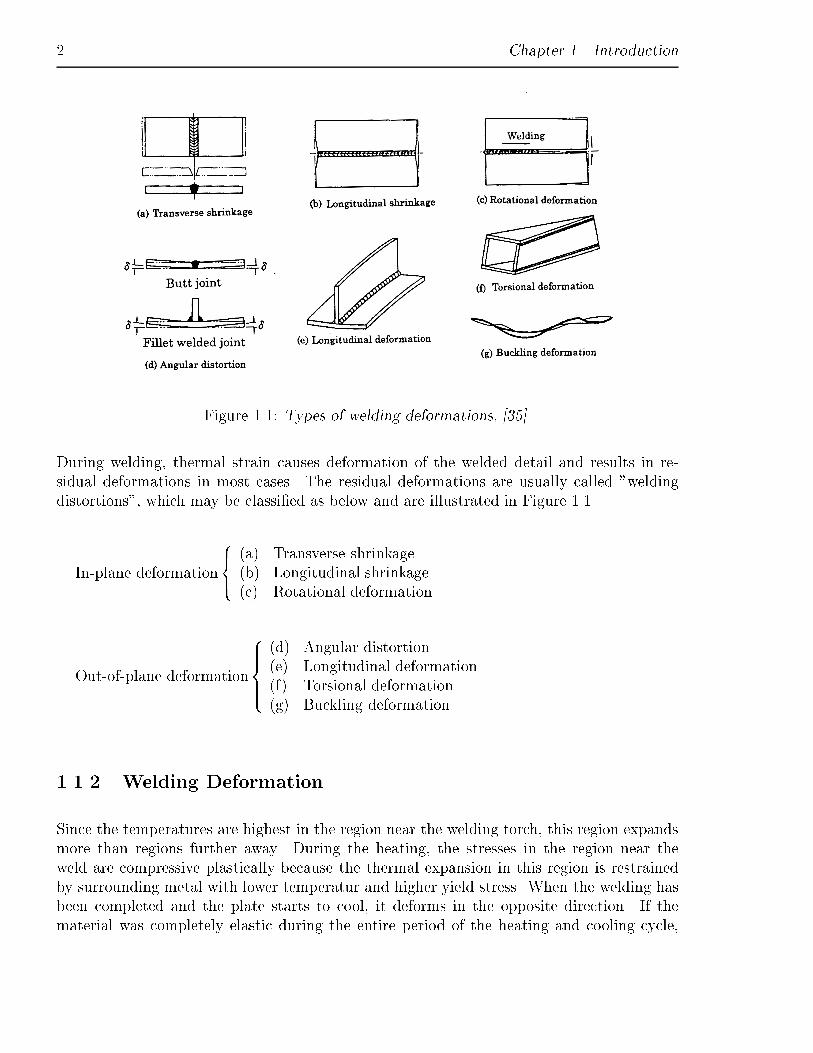
Figure 1.1: Types of welding deformations, [35].
During welding, thermal strain causes deformation of the welded detail and results in re-sidual deformations in most cases. The residual deformations are usually called "weldingdistortions", which may be classi�ed as below and are illustrated in Figure 1.1.
In-plane deformation
8><>:
(a) Transverse shrinkage(b) Longitudinal shrinkage(c) Rotational deformation
Out-of-plane deformation
8>>><>>>:
(d) Angular distortion(e) Longitudinal deformation(f) Torsional deformation(g) Buckling deformation
1.1.2 Welding Deformation
Since the temperatures are highest in the region near the welding torch, this region expandsmore than regions further away. During the heating, the stresses in the region near theweld are compressive plastically because the thermal expansion in this region is restrainedby surrounding metal with lower temperatur and higher yield stress. When the welding hasbeen completed and the plate starts to cool, it deforms in the opposite direction. If thematerial was completely elastic during the entire period of the heating and cooling cycle,

1.1. Overview and Background 3
Figure 1.2: Deformation of a steel plate dur-ing and after welding.
Figure 1.3: Stresses according their origin ina transverse weld in the deck of a 255,000dtw tanker, [18].
the plate would return to its initial shape with no residual distortion. However, for metalslike steel and aluminium plastic deformations occur. As a result of the compressive plasticstrains produced in the regions near the welding zone, the plate continues to deform afterpassing its initial shape, which results in a negative �nal distortion when the plate coolsdown to its initial temperature, as illustrated in Figure 1.2. The deformations may be solarge that the object cannot ful�l its intended function or �t its intended location.
The residual stresses are associated with these deformations. Residual stresses exist in abody when there are no external loads or body forces. One of the sources is the plasticdeformation which occurs in many manufacturing processes. If an initially stress-free bodyis subjected to an arbitrary set of forces, non-uniform plastic deformations may occur. Ifthese loads are removed the body will elastically unload. Plastic deformation deforms someparts of the body more than others. It may be that a stress free-state, after loads have beenremoved, is impossible if the body is to remain continuous. The stresses remaining after allthe loads have been removed are the residual stresses, which are equal to or smaller thanthe yield stress existing after the weld has completely cooled. Residual stresses and weldingdistortion are two faces of the same problem, namely the thermally induced plasticity, andprediction and control of residual stresses and distortions are crucial in manufacture of weldedstructures. The residual stresses also a�ects the fatigue, buckling and yielding strength.
The main objective of this study is to simulate the distortion in ship sections, i.e. withresidual stresses on a macroscale. The residual stresses may have a signi�cant in uence on thestrength of a steel structure. A study by Gell [18] presents results from stress measurementsin the deck of a 255,000 dtw VLCC during manufacture and on the maiden voyage fromScandinavia to the Gulf. The stresses are, according to origin, shown in Figure 1.3, fromwhich it is clear that welding and erection account for the majority of the stresses induces.It should be noted that moderate sea was encountered on the voyage, which explains the
4 Chapter 1. Introduction
low contribution of the wave-induced part to the total stress level.
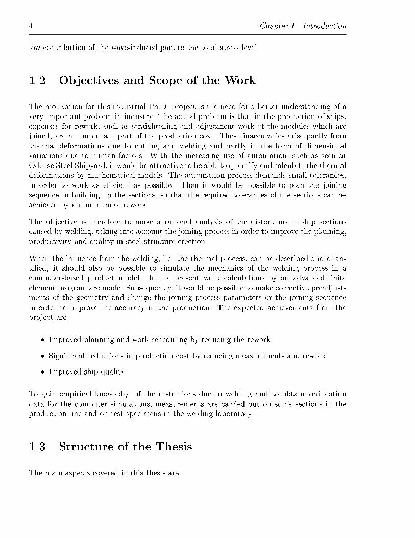
1.2 Objectives and Scope of the Work
The motivation for this industrial Ph.D. project is the need for a better understanding of avery important problem in industry. The actual problem is that in the production of ships,expenses for rework, such as straightening and adjustment work of the modules which arejoined, are an important part of the production cost. These inaccuracies arise partly fromthermal deformations due to cutting and welding and partly in the form of dimensionalvariations due to human factors. With the increasing use of automation, such as seen atOdense Steel Shipyard, it would be attractive to be able to quantify and calculate the thermaldeformations by mathematical models. The automation process demands small tolerances,in order to work as e�cient as possible. Then it would be possible to plan the joiningsequence in building up the sections, so that the required tolerances of the sections can beachieved by a minimum of rework.
The objective is therefore to make a rational analysis of the distortions in ship sectionscaused by welding, taking into account the joining process in order to improve the planning,productivity and quality in steel structure erection.
When the in uence from the welding, i.e. the thermal process, can be described and quan-ti�ed, it should also be possible to simulate the mechanics of the welding process in acomputer-based product model. In the present work calculations by an advanced �niteelement program are made. Subsequently, it would be possible to make corrective preadjust-ments of the geometry and change the joining process parameters or the joining sequencein order to improve the accuracy in the production. The expected achievements from theproject are
� Improved planning and work scheduling by reducing the rework
� Signi�cant reductions in production cost by reducing measurements and rework
� Improved ship quality
To gain empirical knowledge of the distortions due to welding and to obtain veri�cationdata for the computer simulations, measurements are carried out on some sections in theproduction line and on test specimens in the welding laboratory.
1.3 Structure of the Thesis
The main aspects covered in this thesis are
1.3. Structure of the Thesis 5
� Establishment of an empirically based heat ux simulating the heat source
� Experimental investigation of the temperature distribution
� Welding residual stresses
� Measurement of welding-induced residual stresses
� Distortion measurements
� FEM models and parameter study
� Numerical examples
The aspects are presented in 7 chapters composed as follows.
Chapter 2 deals with the welding temperature �eld around the moving heat source, bymeans of the analytical formula given by Rosenthal [48]. An extension for the temperature ux distribution based on a Gaussian distribution is presented. Experimental investigationof the temperature distribution by use of an infrared camera and a comparison with theRosenthal equations are presented, too.
A brief description of residual stresses is given in the beginning of Chapter 3, which deals withthe measurements of residual stresses by use of strain gauges. Before starting to measure andcalculate distortions numerically a simple beam theory is used to obtain some theoreticalinsight into the out-of-plane distortion. This analytical investigation is presented in the endof Chapter 3.
Chapter 4 describes the di�erent measurements which have been carried out. The measure-ments have been made with the focus on both the welding itself and the distortion due tothe actual process.
The beginning of Chapter 5 outlines the theory behind the �nite element program applied,then the numerical parameter study is discussed and last examples of applications are given.
Di�erent parametric expressions for the welding-induced distortion are presented in Chapter6 and compared with the measurements.
Finally, conclusions and recommendations for further work are presented in Chapter 7 andcomments relevant to the project are included.

6 Chapter 1. Introduction
This page is intentionally left blank.
Chapter 2
Welding-induced Temperature Field
2.1 Introduction
To determine the welding mechanics, two di�erent analyses are required, namely heat con-duction and thermal-elastic-plastic analyses. The most signi�cant factors a�ecting bothanalyses are the heat input rate, the moving speed of the heat source, and the thicknessof the plate. Secondary factors which may also a�ect the deformation are the geometry ofthe heating line, the heat input distribution, the initial curvature of the plate and residualstresses from the plate rolling and cutting processes.
A general introduction to thermal stresses can be found in e.g. Benham et al. [3], Boley etal. [6] and Carslaw and Jaeger [7].
The Chapter deals with heat conducting in materials. Temperature pro�les are obtained byexperiments and formulas, di�erent pro�les are compared. A Gaussian heat input distribu-tion is set up.
2.2 Heat Conduction
The fundamental behaviour of heat conduction is that a ux, Q00 (Wm2 ), of energy ows from
a hot region to cooler regions, linearly dependent on the temperature gradient, rT:
Q00 = �krT (2.1)
where k is the thermal conductivity of the material and r = ( @@x; @@y; @@z). It should be
noted that the minus sign is necessary in order to make Q00 positive, because heat is always

8 Chapter 2. Welding-induced Temperature Field
transferred in the direction of decreasing temperature as stated above. The energy requiredto change the temperature of the material is de�ned by another materials parameter, thespeci�c heat c (or enthalpy, H). In terms of the speci�c heat, the thermal ux and adistributed volume heat-source term Q000 (W
m3 ), the conservation of energy in a di�erentialform yields
�c _T �r(krT )�Q000 = 0 (2.2)
where _( ) = ddtwith t being the time parameter and � the density of the material. In order
to solve Eq. 2.2, boundary and initial conditions must be speci�ed. A boundary conditioncan in numerical sence be either absolute (prescribed temperature) or natural (prescribedthermal uxes) and also being a function of time.
The boundary conditions for the heat transfer coe�cient are divided into radiation andconvection. Given a body temperature T in Kelvin, radiation to the surrounding media atthe temperature T0 follows the Stefan-Boltzmann law, so that the temperature di�erencecauses a ux (power loss) given by
Q00rad = ��(T 4 � T 4
0 ) (2.3)
= ��(T 2 + T 20 )(T + T0)(T � T0)
= hrad(T � T0)
Here � is the emissivity, � the Stefan-Boltzmann constant and hrad the resulting temperaturedependent heat transfer coe�cient for radiation.
Given a body with temperature T , surrounded by a uid or gas at temperature T0, heatconvection assumes that a thermal layer exists with the heat transfer coe�cient hcon, so thatthe temperature di�erence across the boundary layer causes a ux, Q00
con, given by
Q00con = hcon(T � T0) (2.4)
If the uid is owing at a velocity v over a plate with a Prandtl number, Pr, and a Reynoldsnumber, Re, then the heat transfer coe�cient by convection hcon can be estimated as, [19]:
hcon = 0:332k
mRe1=3Pr1=3 (2.5)
where k is the thermal conductivity ( WmK
) and m is the thickness of the boundary layer. Theconductance for free convection to air is usually given in the interval 2-10 W
mK, [23].
In the FEM analysis (see Chapter 5), these boundary conditions are applied to the modelby specifying the value of heat transfer coe�cient and the surrounding temperatures atthe elements and nodes respectively, of the skin elements obtained by creating a mesh atthe boundaries of the domain studied. It should be noted that the losses by convection isassumed to be 25 W
m2 .
2.3. Quasi-stationary Temperature Distribution 9
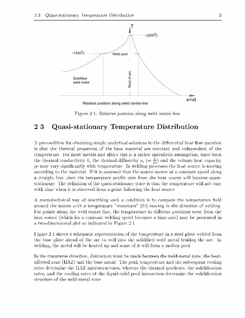
Figure 2.1: Relative position along weld centre line.
2.3 Quasi-stationary Temperature Distribution
A precondition for obtaining simple analytical solutions to the di�erential heat ow questionis that the thermal properties of the base material are constant and independent of thetemperature. For most metals and alloys this is a rather unrealistic assumption, since boththe thermal conductivity k, the thermal di�usivity a, (= k
�c) and the volume heat capacity
�c may vary signi�cantly with temperature. In welding processes the heat source is movingaccording to the material. If it is assumed that the source moves at a constant speed alonga straight line, then the temperature pro�le seen from the heat source will become quasi-stationary. The de�nition of the quasi-stationary state is that the temperature will not varywith time when it is observed from a point following the heat source.
A memotechnical way of describing such a condition is to compare the temperature �eldaround the source with a temperature "mountain" [21] moving in the direction of welding.For points along the weld centre line, the temperature in di�erent positions away from theheat source (which for a constant welding speed becomes a time axis) may be presented ina two-dimensional plot as indicated in Figure 2.1.
Figure 2.1 shows a schematic representation of the temperature in a steel plate welded fromthe base plate ahead of the arc to well into the solidi�ed weld metal trailing the arc. Inwelding, the metal will be heated up and some of it will form a molten pool.
In the transverse direction, distinction must be made between the weld-metal zone, the heat-a�ected zone (HAZ) and the base metal. The peak temperature and the subsequent coolingrates determine the HAZ microstructures, whereas the thermal gradients, the solidi�cationrates, and the cooling rates at the liquid-solid pool interaction determine the solidi�cationstructure of the weld-metal zone.

10 Chapter 2. Welding-induced Temperature Field
Figure 2.2: The three stages in the welding time problem.
The heating in the welding process involves three stages, sketched in Figure 2.2:
1. A transient stage at which the temperature around the heat source is still rising, oftencalled the initiation stage
2. The quasi� stationary stage at which the temperature distribution is stationary in aco-ordinate system moving with the heat source
3. A second transient stage at which the temperature decrease after the welding arc isextinguished
The majority of the thermal expansion and shrinkage in the base material and in the HAZoccurs at the quasi-stationary stage, [13].
The concept of an instantaneous and �xed heat source is widely used in the theory of heatconduction. The assumption implies that the heat is released instantaneously at the time t= 0 in an in�nite medium of the initial temperature T0. Solving Eq. 2.2 with the appropriateboundary and initial conditions yields, for the line source in a wide plate (r � 0), [40]:
T � T0 =J
gk4�texp
"� r2
4at
#(2.6)
where J is the heat input (J), g is the plate thickness, a = k�cand t is the time. r is de�ned
aspx2 + y2.
For the point source in a 3D solid, (R > 0):
T � T0 =J
�c(4�at)3=2exp
"�R2
4at
#(2.7)
R is for the 3D case de�ned aspx2 + y2 + z2. Eqs. 2.6 and 2.7 will provide the required
basis for comprehensive theoretical treatments of heat ow phenomena in welding.
2.3. Quasi-stationary Temperature Distribution 11
2.3.1 Moving Point Source
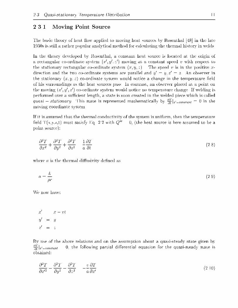
The basic theory of heat ow applied to moving heat sources by Rosenthal [48] in the late1930s is still a rather popular analytical method for calculating the thermal history in welds.
In the theory developed by Rosenthal, a constant heat source is located at the origin ofa rectangular co-ordinate system (x0; y0; z0) moving at a constant speed v with respect tothe stationary rectangular co-ordinate system (x; y; z) . The speed v is in the positive x-direction and the two co-ordinate systems are parallel and y0 = y; z0 = z. An observer inthe stationary (x; y; z) co-ordinate system would notice a change in the temperature �eldof his surroundings as the heat sources pass. In contrast, an observer placed at a point onthe moving (x0; y0; z0) co-ordinate system would notice no temperature change. If welding isperformed over a su�cient length, a state is soon created in the welded piece which is calledquasi � stationary. This state is represented mathematically by @T
@tjx0=constant = 0 in the
moving coordinate system.
If it is assumed that the thermal conductivity of the system is uniform, then the temperature�eld T(x,y,z,t) must satisfy Eq. 2.2 with Q000 = 0, (the heat source is here assumed to be apoint source):
@2T
@x2+@2T
@y2+@2T
@z2=
1
a
@T
@t(2.8)
where a is the thermal di�usivity de�ned as
a =k
�c(2.9)
We now have:
x0 = x� vt
y0 = y
z0 = z
By use of the above relations and on the assumption about a quasi-steady state given by@T@tjx0=constant = 0, the following partial di�erential equation for the quasi-steady state is
obtained:
@2T
@x02+@2T
@y2+@2T
@z2= �v
a
@T
@x0(2.10)
12 Chapter 2. Welding-induced Temperature Field
A main disadvantage of this equation is that the heat source is concentrated at one point. Incontrast, the heat from a torch ame is distributed over a �nite area. Another disadvantageis the assumption that the physical properties of the heated plate are constant. The quasi-stationary solution given by Rosenthal is also unable to treat the transient behaviour nearthe plate edges.
2.3.2 Thick Plate Solution
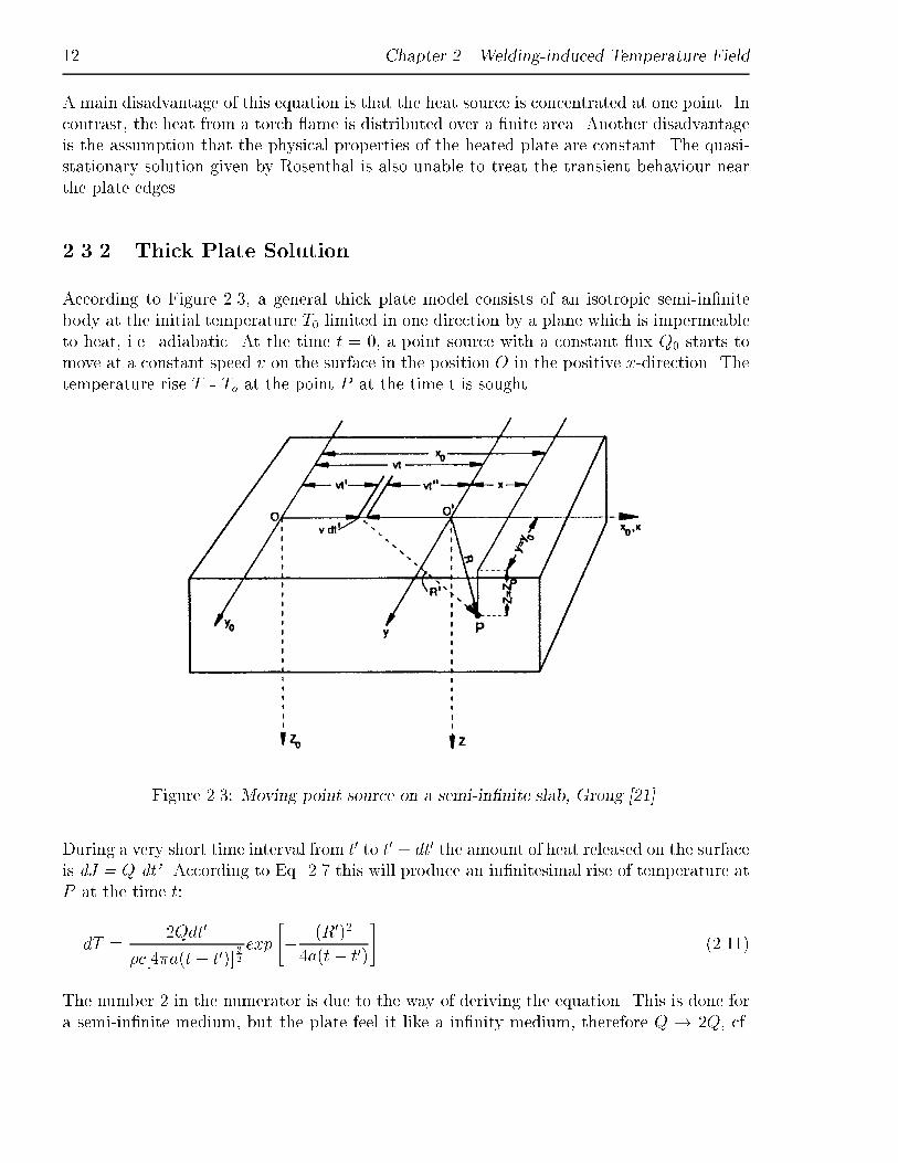
According to Figure 2.3, a general thick plate model consists of an isotropic semi-in�nitebody at the initial temperature T0 limited in one direction by a plane which is impermeableto heat, i.e. adiabatic. At the time t = 0, a point source with a constant ux Q0 starts tomove at a constant speed v on the surface in the position O in the positive x-direction. Thetemperature rise T - To at the point P at the time t is sought.
Figure 2.3: Moving point source on a semi-in�nite slab, Grong [21].
During a very short time interval from t0 to t0 + dt0 the amount of heat released on the surfaceis dJ = Q dt'. According to Eq. 2.7 this will produce an in�nitesimal rise of temperature atP at the time t:
dT =2Qdt0
�c[4�a(t� t0)]3
2
exp
"� (R0)2
4a(t� t0)
#(2.11)
The number 2 in the numerator is due to the way of deriving the equation. This is done fora semi-in�nite medium, but the plate feel it like a in�nity medium, therefore Q ! 2Q, cf.
2.3. Quasi-stationary Temperature Distribution 13
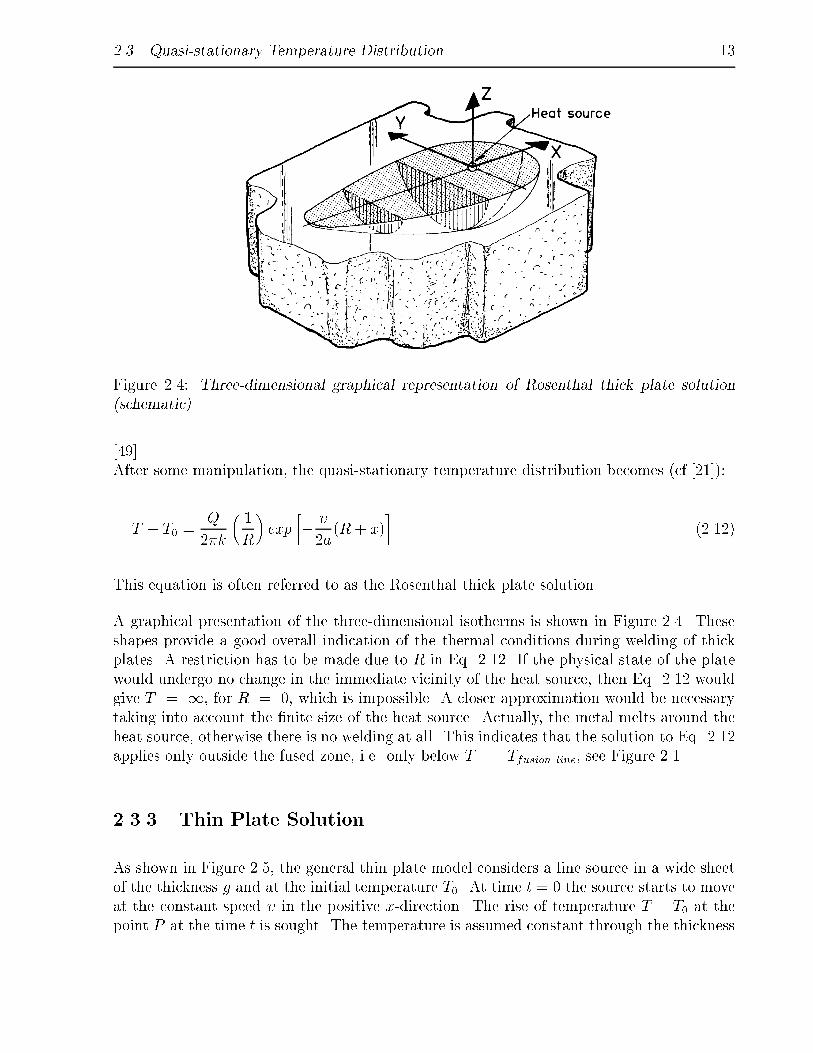
Figure 2.4: Three-dimensional graphical representation of Rosenthal thick plate solution(schematic).
[49].After some manipulation, the quasi-stationary temperature distribution becomes (cf.[21]):
T � T0 =Q
2�k
�1
R
�exp
�� �
2a(R + x)
�(2.12)
This equation is often referred to as the Rosenthal thick plate solution.
A graphical presentation of the three-dimensional isotherms is shown in Figure 2.4. Theseshapes provide a good overall indication of the thermal conditions during welding of thickplates. A restriction has to be made due to R in Eq. 2.12. If the physical state of the platewould undergo no change in the immediate vicinity of the heat source, then Eq. 2.12 wouldgive T = 1, for R = 0, which is impossible. A closer approximation would be necessarytaking into account the �nite size of the heat source. Actually, the metal melts around theheat source, otherwise there is no welding at all. This indicates that the solution to Eq. 2.12applies only outside the fused zone, i.e. only below T = Tfusion line, see Figure 2.1.
2.3.3 Thin Plate Solution
As shown in Figure 2.5, the general thin plate model considers a line source in a wide sheetof the thickness g and at the initial temperature T0. At time t = 0 the source starts to moveat the constant speed � in the positive x-direction. The rise of temperature T � T0 at thepoint P at the time t is sought. The temperature is assumed constant through the thickness

14 Chapter 2. Welding-induced Temperature Field
Figure 2.5: Moving line source in a thin sheet, Grong [21].
of the plate. According to Eq. 2.6, the elementary source, dJ = Qdt0 released in the position�t0 will cause a small rise of temperature dT in the point P at the time t:
dT =Qdt0
gk4�(t� t0)exp
"� r02
4a(t� t0)
#(2.13)
=Qdt00
gk4�t00exp
"� r02
4at00
#(2.14)
where t00 = t� t0 is the time available for conduction of heat over the distance r0 to the pointP . If we refer the position P to that of the heat source at the time t, we shall expect asolution independent of time. This is achieved by changing the co-ordinate system from Oto O'. Hence,
dT =Qdt00
gk4�t00exp
"�(x + �t00)2 + y2
4at00
#
=Qdt00
gk4�t00exp
"��x2a� r2
4at00� �2t00
4a
#(2.15)
where
r =qx2 + y2 (2.16)
2.3. Quasi-stationary Temperature Distribution 15
For integration of all contributions from t" = t (t'=0) to t" = 0 (t' = t), the followingnotation is introduced:
(r�)2 =�2r2
4a2; ! =
�2t00
4a(2.17)
Furthermore,
t00 =4a
�2!; dt00 =
4a
�2d!;
r2
4at00=
r�2
4!(2.18)
Substituting these parameters into Eq. 2.15 yields by integration:
T � T0 =Q
g4�kexp
���x2a
� Z !=�2t4a
!=0exp
"�(r
�)2
4!� !
#d!
!(2.19)
As Grong [21]:
Z 1
0exp
"�(r
�)2
4!� !
#d!
!= 2K0(r
�) = 2K0
��r
2a
�(2.20)
where K0(r�) is the modi�ed Bessel function of the second kind and zero order. Hence, the
general thin plate solution can be written as
T � T0 =Q
2g�kexp
���x2a
� "K0
��r
2a
�� 1
2
Z 1
!exp
"�(r
�)2
4!� !
#d!
!
#(2.21)
When ! (= �2 t00
4a) is su�ciently large (i.e. when the welding has been performed over a
su�cient period), we obtain the pseudo-steady state temperature distribution:
T � T0 =Q
2g�kexp
���x2a
�K0
��r
2a
�(2.22)
Eq. 2.22 is referred to as the Rosenthal thin plate solution. It follows that this model isapplicable to all types of welding processes (including electron beam, plasma arc and laserwelding), provided that a full through-thickness penetration is achieved at one pass and thatno thermal gradient through thickness can be assumed. It is seen from Figure 2.6 that theisotherms behind the heat source are increasingly elongated upstreams.

16 Chapter 2. Welding-induced Temperature Field
Figure 2.6: Graphical representation of Rosenthal thin plate solution (schematic).
2.3.4 Medium Thick Plate Solution
In a real welding situation the assumption about three-dimensional or two-dimensional heat ow inherent in the Rosenthal equations is not always ful�lled because of variable tempe-rature gradients in the thickness, the z-direction of the plate.
The general medium thick plate model considers a point heat source moving at a constantspeed across a wide plate of the �nite thickness g. According to investigations made byRosenthal [47] it is reasonable to assume that the plate surfaces are impermeable to heat.Thus, in order to maintain the net heat ux through both boundaries equal to zero, it isnecessary to account for mirror re ections of the source with respect to the planes z=0 andz=g. This can be done by use of the method of images (�ctitious sources). The contributionsof the mirror re ections are of the form
Q
2�kexp
���x2a
�1
Ri
�exp
��Ri
2a
�(2.23)
2.3. Quasi-stationary Temperature Distribution 17
where
Ri =qx2 + y2 + (z � 2id)2 (2.24)
Hence, the solution reads
T � T0 =Q
2�kexp
���x2a
� 1Xi=�1
exp(��Ri
2a)
Ri(2.25)
In accordance with [47] the solution of Eq. 2.25 can be transformed into a Fourier series:
T � T0 =Q
2g�kexp
���x2a
�8><>:K0
�r
2a+ 2
1Xi=�1
K0
264rvuut� �
2a
�2+
�i
g
!2375 cos�iz
g
9>=>; (2.26)
The similarity between Eqs. 2.26 and 2.22 (thin plate solution) is obvious, for points locatedsu�ciently far away from the heat source centre, i.e. large values of r. For small values of r,i.e. points close to the heat source centre, the thermal conditions will be similar to those in athick plate. However, at intermediate distances from the heat source, the quasi-steady statetemperature distribution will deviate signi�cantly from that observed in thick plate or thinplate welding because of variable temperature gradients in the through-thickness directionof the plate. In this "transition region", the thermal solution is only de�ned by the mediumthick plate solution, Eq. 2.26, see also Section 2.4.
For the comparison in this chapter, only the equations for the 2D (thin plate) and 3D (thickplate) solutions are used.
2.3.5 Other Formulas
In the literature various types of quasi-stationary temperature �elds are presented. Most ofthem are a slight modi�cation of Rosenthal's Eqs. 2.12 and 2.22. Adams [1] e.g. uses theequation presented by Rosenthal, except that the positive x is opposite to the direction ofmotion of the source.
Satoh [52] presented a similar expression to Eq. 2.22 taking into account the heat radiation.This is done by using hrad, for calculating the temperature �eld, i.e. as a modi�cation of thethin plate solution:
T � T0 =Q
2�gkexp
��vx2a
�K0
"r
s2hradkg
+ (v
2a)2#
(2.27)
18 Chapter 2. Welding-induced Temperature Field
where hrad is the heat radiation coe�cient de�ned in Eq. 2.4. Here hrad is set to 58:8J
m2�s�K,
[51]. This formula gives a temperature pro�le, which is very close to the pro�le for theRosenthal's 2D solution.
Hrivnak [25] set up two rather simple formulas for the temperature:
T � T0 =
s2
�e
Q
2g�crv(2.28)
for thin plates and
T � T0 =2
�e
Q
�cr2v(2.29)
for thick plates. Here e is basis of natural logarithms, e = 2.72. As Eq. 2.27, this equationgives a very narrow heat pro�le. These expressions are compared with those obtained bythe infrared measurements, presented later in this chapter.
2.4 Experimental Investigation of the Temperature Dis-
tribution
This section deals with analytical, numerical and experimental determination of the tempe-rature distribution. Experimental work is vital because it is impossible, from �rst principles,to express in mathematical terms the nature of a welding arc. An experimental basis isneeded for interpretation and correlation of the mathematical representations with the "realworld".
Single beads deposited on pieces of mild steel and in V-grooves by means of metal activegas ux cored wire (MAG FCW) welding at two di�erent heat source travelling speedsare examined with regard to the temperature distribution outside the weld pool. The heatdistribution is measured by use of infrared camera. The results are compared with predictionsderived from the equations in Sections 2.3 and 2.6 and numerical results obtained by FEMcalculations. Observed deviations from the behaviour predicted by Rosenthal's models arediscussed.
The heat conditions during welding account for most of the phenomena encountered sub-sequently; shrinkage, residual stresses, metallurgical changes, physical changes, chemicalmodi�cations, etc. While experiments reveal the particular features of a speci�c process,a theory permits the establishment of general laws and thus contributes to the fundamen-tal knowledge of the process. Both are necessary to improve the simulation of the welding
2.4. Experimental Investigation of the Temperature Distribution 19
process. Therefore, information about the temperature in relation to location, time, andwelding conditions must be obtained.
As before mentioned, Rosenthal [47], [48] and Rykalin [49] modelled the heating e�ect ofa moving heat source as a point source, i.e. all the energy input is at a point. In a FEMmodel, this could be accomplished by specifying a thermal load at a node. The most notabledi�erence between a FEM approximation and Rosenthal solution is that the temperatureat the point source is in�nite in the Rosenthal solution, whereas it is �nite in the FEMapproximation. The explanation is that, in the Rosenthal solution, a �nite amount of energyis put into zero volume at the point whereas, in the FEM approach, a �nite amount of energycan be put into the elements in the heating zone.
Near the point source, the Rosenthal solution varies exponentially with the position. TheFEM solution has a polynomial dependence on position which is due to the polynomialbasis functions. If the �nite element mesh size goes to zero, then the FEM approximationcompared to the Rosenthal solution becomes more accurate. The advance of FEM is thatthe energy input can be distributed to a zone representing the arc. It is preferable to use anaccurate approximation to the energy distribution in the arc. A rather good experimentalbackground is invaluable for suggesting which kind of approximation is liable to be used,without loss of accuracy, and for arriving at equations which are not too di�cult to use inthe practical welding research.
2.4.1 2D or 3D Heat Flow
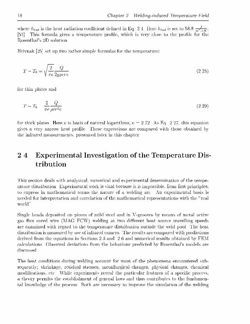
The heat distribution during welding is governed by material constants such as the density,the speci�c heat, the thermal conductivity and the surface transmission coe�cient. Unfor-tunately, the experimental determination of some of these constants is very di�cult and, inaddition, they vary sometimes very steeply with the temperature. In the simple expressiondealt with until now, two types of heat ow occur: Two-dimensional (thin plate) and three-dimensional (thick plate) are considered. The heat ow is sketched in Figure 2.7. Thickness
Figure 2.7: Scheme of heat ow. a) 3D ow, b) 2D ow.
itself cannot always "predict" the dimension of the formula. For instance, a submerged arc

20 Chapter 2. Welding-induced Temperature Field
passes on a 50mm steel plate using a current of 900amp and a voltage of 27V at 0.2m/mininvolves essentially two-dimensional heat ow, whereas a 150amp 20V passing a by MAGwelding on a 20mm thick plate at 0.4m/min will cool as if the plate was in�nitely thick.Thus the choice of equation to be used for the temperature �eld also depends on the speci�cwelding conditions.
To prove this behaviour the cooling rate dTdt
is considered. Rosenthal [47] derived the coolingrate for the 2D plate from Eq. 2.22, by looking along the weld line, i.e. y = 0 and x = -�t.The following expression is obtained:
dT
dt= �2�k�cg2
�
Q
!2
(T � T0)3 (2D) (2.30)
where as before k is the conductivity of the metal, � is the density, c is the speci�c heatcapacity, g is the thickness of the plate, � is the velocity of the torch, Q is the net heat e�ectin W , and T and T0 are the actual and initial temperatures, respectively.
The rate of cooling for a thick plate can be derived from Eq. 2.12. If the observations arelimited to the surface and along the weld, the distance R is simply the distance �t coveredby the arc in a given period of time t. The cooling rate is derived to be
dT
dt= �2�k �
Q(T � T0)
2 (3D) (2.31)
The right hand-side of Eq. 2.31 is constant for a given temperature, material, heat input andspeed, hence the left-hand side must also be constant. By dimensional analysis the coolingrates are normalised by the cooling rate for the thick plate, Eq. 2.31. Thus of course for thethree-dimensional plate
dTdt
�2�k �Q(T � T0)2
= 1 (3D) (2.32)
and for the two-dimensional plate the following formula is obtained:
dTdt
�2�k �Q(T � T0)2
=2�k�cg2
��Q
�2(T � T0)
3
2�k�c �Q(T � T0)2
= �c�
Qg2(T � T0) = �g2 (2D) (2.33)
A dimensionless thickness �g for the 2D case is de�ned as
�g = g
s�c�
Q(T � T0) (2.34)

2.4. Experimental Investigation of the Temperature Distribution 21
From the dimensionless cooling rates obtained above it is seen that, for the thick plate, Eq.2.32, it is exactly 1, whereas the dimensionless cooling rates for the thin plate vary with thedimensionless thickness �g, in the power of 2. The two formulas for the dimensionless coolingrate are plotted in Figure 2.8 .The dotted line illustrates the behaviour in the transition zone, [1], i.e. the intermediate
Figure 2.8: Dimensionless cooling rate as a function of the dimensionless plate thickness �g.
zone between the validity area for the thin plate solution and the thick plate solution. FromEq. 2.34 the transition thickness, gtransition, is de�ned by
gtransition =g
�g=
1q�c �
Q(T � T0)
(2.35)
By Eq. 2.35 it can be stated that
gtransition > gactual =) 2D (2.36)
gtransition < gactual =) 3D (2.37)

22 Chapter 2. Welding-induced Temperature Field
Using Figure 2.8 it can also be stated that
�g � 0:9 =) 2D (2.38)
�g � 1:2 =) 3D (2.39)
For the submerged arc and MAG welding mentioned in the beginning of this section it isassumed that the materials parameters are � = 7850 kg
m3 , c = 449 JkgK
, the e�ciency � = 0.8
and that the actual temperature Tactual, is 5400C, as in [1], i.e. a little away from the heat
source centre.
�g(submerged arc welding) = 0:88 � 0:9 i.e. 2D solution valid (2.40)
�g(MAG welding) = 1:28 � 1:2 i.e. 3D solution valid (2.41)
By the formulas Eq. 2.36 and Eq. 2.37 it can be determined whether the heat ow fordi�erent types of welding can be calculated as a 2D or a 3D problem.
In order to illustrate the in uence of the welding speed, another example using Rosenthal2D-equation is given below. Only the speed is changed and all other parameters are keptconstant. These parameters are: Q = 5625W, vtorch = 0.0067m
s, k = 46 W
mK, c = 449 J
kgK
and � = 7850 kgm3 . The materials parameter are found in the literature and they are used in
general in the following discussing Rosenthal's equations.
The speed of welding a�ects the shape of the isotherms. The lower the speed, the moreelongated the isotherms. This is illustrated in Figure 2.9. Increasing current intensity wille.g. widen the HAZ without changing the shape of the isotherms.
Figure 2.9: Isotherms in the welding line (y = 0) as a function of the welding speed, obtainedby Rosenthal 2D equation. Due to the point in�nity the curves are truncated at T = 2500oC.

2.4. Experimental Investigation of the Temperature Distribution 23
Table 2.1: Experimental data
Plate dimension 500 x 120 x 22 [mm] & 500 x 120 x 9 [mm]Welding method MAG FCW
Voltage 30 VCurrent 250 amp
Welding velocity 400mmmin
(300mmmin
for V-groove)Reference line A transverse through the heat sourceReference line B longitudinal through the heat sourceReference line C 10 mm beside the heat sourceReference line D 20 mm beside the heat sourceImage logging 1 per second
2.4.2 Infrared Measurements
Experiments have been carried out on the steel quality SS400 (�tensile � 400 MPa), withtwo di�erent thickness' and two di�erent welding speeds. The welding parameters are shownin Table 2.1. The weldings are bead-on-plate and V-groove. Each thermal history of thebeads is stored separately on the PC hard disk by a NEC (Nippon Electric Corporation)TH3100MR thermotracer IR measurement equipment. Images have been taken on both theupper and the lower surface of the test plate. Hence, it should be possible to distinguishwhether the heat ow is 2D or 3D. Each IR image, as those shown in Figure 2.10 andFigure 2.13, has 250 x 250 pixels and contains information about the temperature. Thetemperatures along any arbitrary lines in these images can be tabulated and displayed.Here, a line transverse 20mm abaft the heat source has been drawn and longitudinal lineshave been drawn through the centre and 10mm and 20mm next to the centre.
2.4.3 V-groove
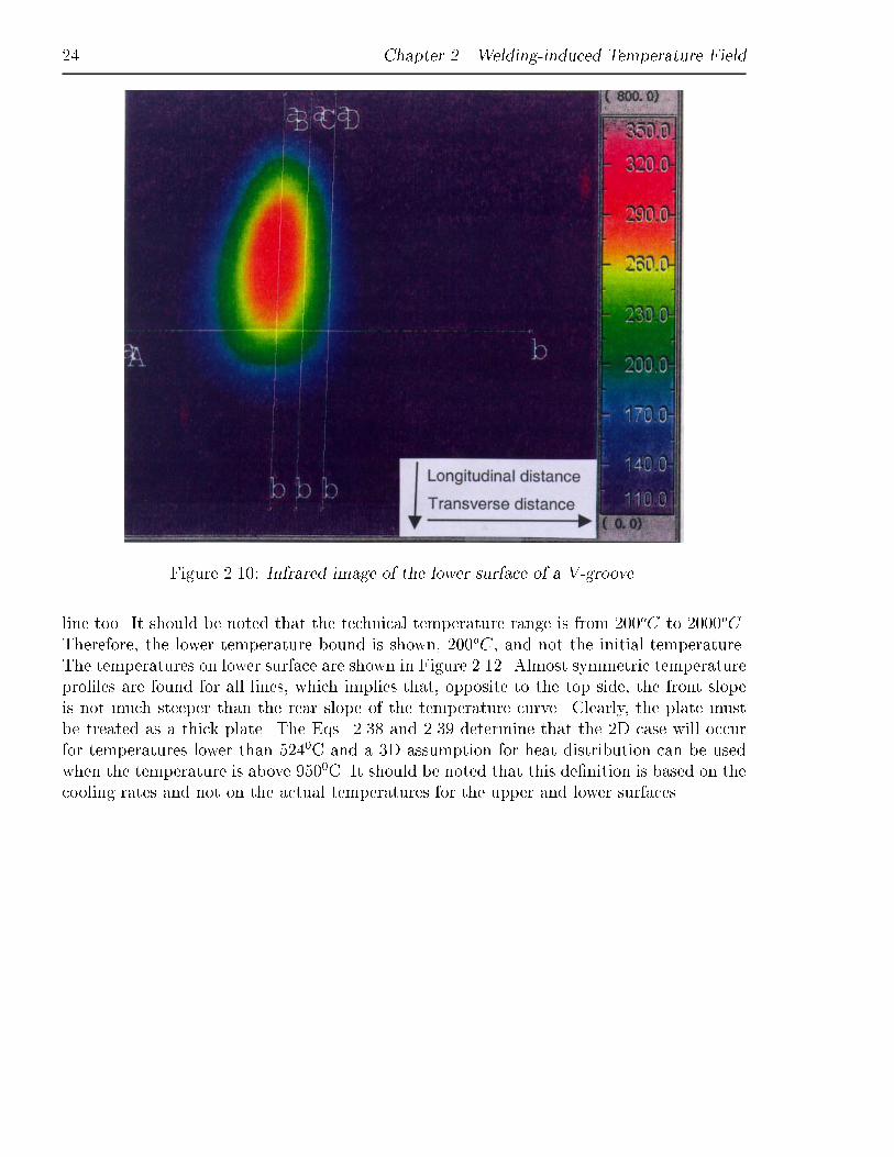
In the following a 60o V-groove in a 22mm thick steel plate is considered. Figure 2.11shows the temperature variation transversely and longitudinally to the weld line, plotted asa function of the longitudinal and transverse distance to the source centre. As seen fromthis top image of the V-groove, the transverse temperature line, taken 20mm behind theheat source centre, has a symmetric pro�le, and the longitudinal line through the centrepoint shows that the rise of temperature in front of the heat source is steeper than thefall of temperature behind the source. The maximum temperature is here only measured toapproximately 1300oC, which is obviously too low because it is much below the melting pointof the steel. This is an inaccuracy of several hundreds degrees. This inaccuracy may be dueto an error in the speci�c test case, because it is not seen in the following measurements. Thesame tendency in temperature slope is seen for the line 10mm and 20mm away from the centre
24 Chapter 2. Welding-induced Temperature Field
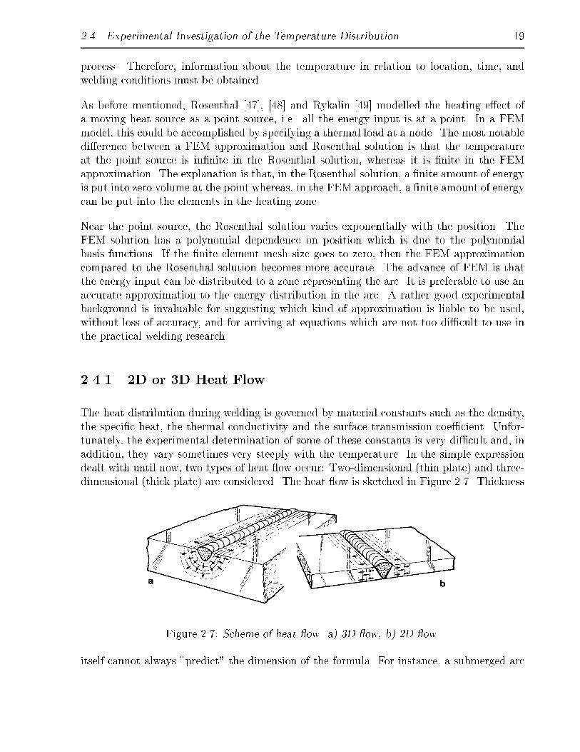
Figure 2.10: Infrared image of the lower surface of a V-groove.
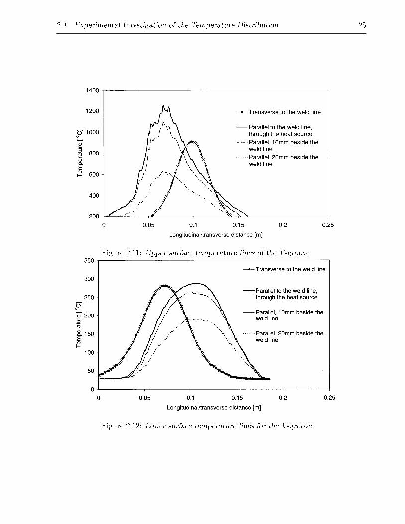
line too. It should be noted that the technical temperature range is from 200oC to 2000oC.Therefore, the lower temperature bound is shown, 200oC, and not the initial temperature.The temperatures on lower surface are shown in Figure 2.12. Almost symmetric temperaturepro�les are found for all lines, which implies that, opposite to the top side, the front slopeis not much steeper than the rear slope of the temperature curve. Clearly, the plate mustbe treated as a thick plate. The Eqs. 2.38 and 2.39 determine that the 2D case will occurfor temperatures lower than 5240C and a 3D assumption for heat distribution can be usedwhen the temperature is above 9500C. It should be noted that this de�nition is based on thecooling rates and not on the actual temperatures for the upper and lower surfaces.
2.4. Experimental Investigation of the Temperature Distribution 25
Figure 2.11: Upper surface temperature lines of the V-groove.
Figure 2.12: Lower surface temperature lines for the V-groove
26 Chapter 2. Welding-induced Temperature Field
Figure 2.13: Infrared image of upper surface of a bead-on-plate test weld.
2.4.4 Bead on Plates
The temperature pro�le around the heat source, moving at a velocity of 400mm/min whenlaying a bead on a 9mm thick steel plate, is shown in Figure 2.13. For modelling the heatsource the semiaxis of the ellipse limiting the main temperature area for this steady-statesource is read to be 5mm in the front, 5mm to the sides and 20mm in the rear. Thecurves obtained from the IR measurements, Figure 2.14, show a very steep front and a peaktemperature, for the line through and along the weld centre, of 17000C. A little hump isseen on the rear side. The occurrence of this indicates an uncertain temperature distributionin the weld pool. Figure 2.14 also shows that the width of the heat distribution is rathernarrow as the temperature line of 20mm beside the source centre only rises to approximately4000 C. Again the temperature curves for the lower surface of the plate, Figure 2.15, almosthave a symmetrical temperature pro�le.
In order to illustrate the steady-state behaviour of the moving heat source, 16 sequentialimages were taken. They are shown in Figure 2.16. The travelling speed of the torch inFigure 2.16 is 300mm/min. The interval between each picture is 4 secs. It is seen from the

2.4. Experimental Investigation of the Temperature Distribution 27
Figure 2.14: Upper surface temperature lines for the 9mm plate, torch speed 400 mm/min.
Figure 2.15: Lower surface temperature lines for the 9 mm plate, torch speed 400 mm/min

28 Chapter 2. Welding-induced Temperature Field
Figure 2.16: 16 sequential images (snapshots) for the moving heat source on the surface ofthe 9mm thick plate.
images that the temperature distribution is to a high degree a steady-state distribution. Itcan also be seen that the cooling rate is rather high because the last image, taken half aminute (24 secs) after the torch centre has passed out of the 150mm x 150mm picture area,has almost cooled down to a uniform temperature.
The same pattern is observed for the 22mm plate as for the 9mm plate. In the middle(centre) there is a little hump. The maximum temperature measured is approximately17000C. The surface temperature (the arc side) can be seen in Figure 2.17 and the lowersurface temperature pro�les are shown in Figure 2.18. The transverse temperature pro�lesare symmetric as expected. However, the pro�les for the three parallel lines are asymmetricwith the steepest slope in the rear. This can be caused by the observed heat front delay of3 secs, from the upper to the lower surface in this 22mm thick plate.

2.4. Experimental Investigation of the Temperature Distribution 29
Figure 2.17: Upper surface temperature lines of the 22mm plate, speed 300mm/min.
Figure 2.18: Lower surface temperature lines of the 22mm plate, speed 300mm/min.

30 Chapter 2. Welding-induced Temperature Field
Figure 2.19: Temperature curves along the X-axis through the centre of the heat sourcedoing the V-groove in a 22mm thick plate.
2.5 Comparison
2.5.1 V-groove
This plate has a thickness of 22mm but with the 600 groove it is simulated as a 2D plate.However, Figure 2.19 shows that the Rosenthal 2D Eq. 2.22 gives too low temperature valuesand they do not even �t at temperatures up to 7000C, as calculated in Section 2.5.3, butonly up to approximately 3000C. Hrivnak's Eqs. 2.28 and 2.29 seem to be less useful, due tothe low temperature level away from the centre and the much to narrow temperature pro�le.Furthermore the equation gives a symmetric heat pro�le. The equation given by Satoh, Eq.2.27, taking into account the heat loss factor gives a narrow temperature pro�le, too, whichis almost the same as the Rosenthal 2D. So, the heat loss do not have a signi�cant in uenceon the temperature level.
The generally best curve for the temperature curves around the V-groove obtained by IR isthe 3D equation given by Rosenthal, Eq. 2.12. This was to be expected as the measuredtemperatures were di�erent on the upper and on the lower surface. Using Eqs. 2.36 and 2.37it shows up that the 3D solution for temperatures should be used for temperatures above1000oC, i.e. adjacent to the heat source.

2.5. Comparison 31
2.5.2 9mm Plate
In Figure 2.20 and Figure 2.21 various predictions are shown for the heat ow in the 9mmplate. The Rosenthal 2D solution, Eq. 2.22, is seen to give the best approximation tothe experimentally obtained temperature curve. It is seen that the 2D Rosenthal solutionapproaches the measured temperature pro�le rather well, although the curve is conservative.
Figure 2.20: Temperature curves along the X-axis through the centre, 9mm thick plate.
In order to get temperature lines for the lower surface of the plate, the 3D assumptions areused. These equations take into account the plate thickness as a third co-ordinate in thetemperature distribution. The results for the lower surface are presented in Figure 2.22. TheRosenthal 3D solution, Eq. 2.12, gives here too low upper surface temperatures. For thelower surface, Hrivnak, Eq. 2.29, gives a much too di�erent temperature pattern and it istherefore not shown in Figure 2.22.
Whether the best equation for the temperature distribution is Rosenthal's 2D or 3D equationcan be discussed, cf. Figure 2.21. Using the Eq. 2.36, gtransition is calculated to 0.011m forat temperature of 2000oC which is higher than the actual thickness of 0.009m therefore thetemperature distribution for this 9mm should be calculated with a 2D solution.
The Rosenthal 3D equation can also be used for obtaining the lower surface temperature. Asshown in Figure 2.22 this equation approaches the infrared temperature curves for the linethrough the heat source, 10mm and 20mm beside the weld centre line, rather well for the

32 Chapter 2. Welding-induced Temperature Field
Figure 2.21: Upper surface temperature curves along the X-axis 10mm beside the sourcecentre in the 9mm thick plate.
line through the source centre, but the temperature "bell" is too narrow beside the source.This di�erence is obvious due to the fact that to small a temperature level is obtained bythe IR camera at the lower surface side.
The calculation based on the cooling rates states that a 2D solution could be used, but thelower surface di�er signi�cantly from the upper surface temperature which indicates thatthere is a signi�cant temperature gradient through the plate and hence a three dimensionalheat ow.
2.5.3 22mm Plate
In Figure 2.23 the results of the calculation with the Rosenthal 3D solution in a 22mm thickplate are shown, together with the �ltered infrared measurements. The �gure shows thatthe 3D solution does not have the same accuracy as for the 9mm plate, but it is usable. The�g is at T = 1
2Tmelting equal to 1.25mm which assumes a three-dimensional heat ow what
was to be expected too.

2.6. Heat Source Model 33
Figure 2.22: Temperature curves along the X-axis for the lower surface, 0, 10mm and 20mmbeside the source centre in the 9mm thick plate, �ltered IR measurements.
2.6 Heat Source Model
From the literature, e.g. [11], [20], [25], [29], [31], [38], [43], [44] and [50], it is apparent thatmuch research is in progress aiming at de�ning a reliable heat source model for the weldingprocess.
Knowledge of the heat transfer from the arc to the electrode is essential for determinationof the extent of melting and the subsequent solidi�cation pattern. Jog et al: [29] set upnumerical and empirical models for the variation in the electric potential, the temperaturedistribution, and the electrode heat uxes.
In the present work is the source a controllable moving surface or volumetric heat source,applied to speci�c elements. The source load is developed so the start and stop position canbe de�ned by the user.
2.6.1 Distributed Heat Source
However, Rosenthal's analysis is not able to model the temperatures in the HAZ, and espe-cially at the torch centre, because the Rosenthal formula here gives an in�nity value. Pavelicet al. [44] �rst proposed (cf. Goldak [20]) that the heat source should be distributed. Theysuggested a Gaussian "disc" distribution of ux deposit on the surface of the work-piece.
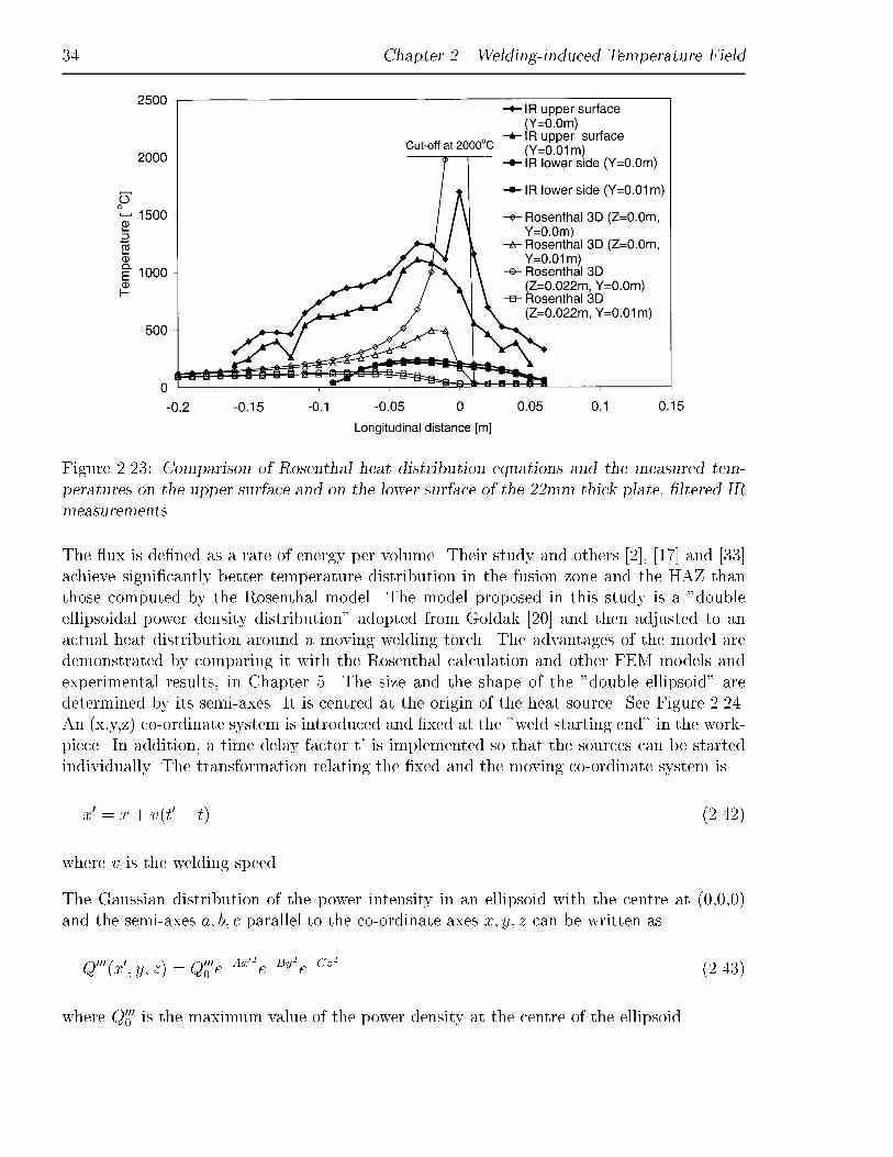
34 Chapter 2. Welding-induced Temperature Field
Figure 2.23: Comparison of Rosenthal heat distribution equations and the measured tem-peratures on the upper surface and on the lower surface of the 22mm thick plate, �ltered IRmeasurements.
The ux is de�ned as a rate of energy per volume. Their study and others [2], [17] and [33]achieve signi�cantly better temperature distribution in the fusion zone and the HAZ thanthose computed by the Rosenthal model. The model proposed in this study is a "doubleellipsoidal power density distribution" adopted from Goldak [20] and then adjusted to anactual heat distribution around a moving welding torch. The advantages of the model aredemonstrated by comparing it with the Rosenthal calculation and other FEM models andexperimental results, in Chapter 5. The size and the shape of the "double ellipsoid" aredetermined by its semi-axes. It is centred at the origin of the heat source. See Figure 2.24.An (x,y,z) co-ordinate system is introduced and �xed at the "weld starting end" in the work-piece. In addition, a time delay factor t' is implemented so that the sources can be startedindividually. The transformation relating the �xed and the moving co-ordinate system is
x0 = x + v(t0 � t) (2.42)
where v is the welding speed.
The Gaussian distribution of the power intensity in an ellipsoid with the centre at (0,0,0)and the semi-axes a; b; c parallel to the co-ordinate axes x; y; z can be written as
Q000(x0; y; z) = Q0000 e
�Ax02e�By2
e�Cz2
(2.43)
where Q0000 is the maximum value of the power density at the centre of the ellipsoid.

2.6. Heat Source Model 35
Figure 2.24: Double ellipsoidal heat input distribution, (Wm3 ).
Conservation of energy requires that
Q = 4Z 1
0
Z 1
0
Z 1
0Q0000 e
�Ax02e�By2
e�Cz2
dx0dydz (2.44)
Note that the integration is only obtained in the interval 0 to 1, i.e. only over one eight ofthe volume, therefore is Eq. 2.44 multiplied by 4 as Q relates to half the volume. EvaluatingEq. 2.44 yields
Q0000 =
2QpABC
�p�
(2.45)
To evaluate the constants, A,B,C, the semi-axes of the ellipsoid a,b,c in the directions x',y,zare de�ned so that the power density falls to 0.05Q000
0 on the surface of the ellipsoid. In thex direction:
Q000(a; 0; 0) = Q0000 e
�Aa2 = 0:05Q0000 (2.46)
Hence,
A =ln20
a2' 3
a2(2.47)
36 Chapter 2. Welding-induced Temperature Field
Similarly,
B ' 3
b2(2.48)
C ' 3
c2(2.49)
Substituting A,B,C from Eqs. 2.47 to 2.49 and Q0000 from Eq. 2.45 into Eq. 2.43 gives
Q000(x0; y; z) =6p3fQ
abc�p�e�3x02
a2 e�3y2
b2 e�3z2
c2 (2.50)
where f is �nal modi�cation for taking into account a fraction of the heat deposited in thefront ff (x'>0) and the rear fr (x'<0). Note that ff + fr = 2. This is done because thetemperature gradient in front of the heat source is steeper than in the tailing edge. Therefore,two ellipsoidal sources are combined as shown in Figure 2.24, one for the front half and onefor the rear half. This is done by using two values for a, a1 and a2 for the front and therear part, respectively. The mathematical expression for the Gaussian heat distribution iscoded directly in the input �le for the used FEM program, see Chapter 5. In this �le theheat input, the welding speed, the fraction values ff , fr the semi-axis and the start andstop positions for the straight welding line has to be given. The subroutine is included inAppendix B.
2.7 Summary
In this chapter no attempts have been made to develop new analytical solutions to thetemperature �eld during welding, but the chapter has veri�ed that the expressions set upby Rosenthal are useful in general engineering practice. The Rosenthal's analysis is ratherinaccurate for temperatures in or near the heat-a�ected zone. In zones where the temperatureis less than half the melting point Rosenthal's solution can give quite accurate results.
In general, the 3D solution should be used for all plates which are not sheets. However,the assumptions for the 3D equation are not ful�lled, because the boundary for the surfaceopposite to the arc side is not adiabatic as it should be. Equations for cooling rates can beused in determining whether the 2D or 3D solution should be used.
The 2D solution gives a heat distribution which is too narrow compared to the infraredsurface measurements for the bead on the plate. 3D solution shows the right pattern butthe overall temperature level is too low.
The heat source applied later in this study is the Gaussian double ellipsoidal power densitydistribution, adjusted to the actual heat distribution around the moving heat torch. This

2.7. Summary 37
power density distribution was selected, rather than the Rosenthal's temperature distribu-tions, because the thermal load should be added to the �nite element analysis elements as a ux, and not as a prescribed temperature �eld.
In general it can be stated that regions with high temperatures i.e. adjacent to the heatsource should be calculated by a 3D solution, and the far �eld could be approximated by2D heat ow solutions. Common for both heat- ow solutions are that the temperature levelshows the best accordance with the experimental obtained temperatures for temperaturesbelow the half of the melting temperature. Goldak [20] e.g. states that the temperature ofthe workpiece should be less than 20% of the melting point, before the Rosenthal's solutionscan give quite accurate results.

38 Chapter 2. Welding-induced Temperature Field
This page is intentionally left blank.
Chapter 3
Welding Residual Stresses
3.1 Introduction
Like other processes involving heating and cooling such as for instance preheating and amebending, welding produces thermal strains and stresses. In the past, many attempts havebeen made to investigate plate distortions due to welding, e.g. [26], [27], [35], [41] and[62]. These works cover many practical aspects of the process, but are based mainly onexperimental data. Some of the authors have also treated welding distortions theoretically,but due to the complexity, it is di�cult to analyse the process, which is highly non-linearand involves plastic deformations and high temperatures varying in both time and space.Therefore, analytical and/or numerical solutions of the thermoelastic-plastic problem arekey factors for the further innovation of ship building technology.
To illustrate physically how residual stresses are formed during welding, a simple case ofa bead �llet on a plate will be described. Figure 3.1 shows schematically the changes intemperature and stresses during the welding process. The welding arc, which is movingat a speed v, is located at the origin O as shown in Figure 3.1(a). Figure 3.1(b) showsthe temperature distribution at several cross- sections. Along section A-A, which is aheadof the welding arc, the temperature change due to the welding �T is almost zero. Alongsection B-B, which crosses the welding arc, the temperature change is extremely rapid andthe distribution is very uneven as also discussed in Chapter 2. Along section C-C, whichis some distance behind the welding arc, the temperature change becomes more even , and�nally, at section D-D, which is very far from the welding arc, the temperature change dueto welding has vanished.
Figure 3.1(c) shows the distribution of longitudinal stresses, �x, along these sections. Normalstresses in the y-direction, �y, and shearing stresses, �xy, also exist, but are usually muchsmaller than �x. In front of the welding, section A-A, the thermal stresses due to welding arealmost zero. Because molten metal does not support a load, stresses underneath the welding
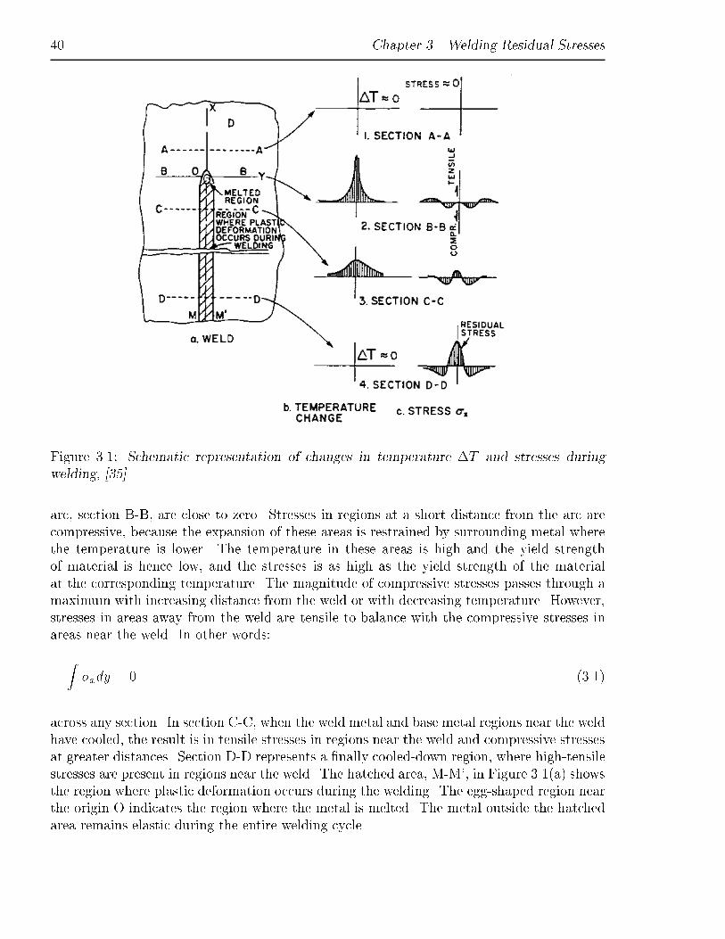
40 Chapter 3. Welding Residual Stresses
Figure 3.1: Schematic representation of changes in temperature �T and stresses duringwelding, [35].
arc, section B-B, are close to zero. Stresses in regions at a short distance from the arc arecompressive, because the expansion of these areas is restrained by surrounding metal wherethe temperature is lower. The temperature in these areas is high and the yield strengthof material is hence low, and the stresses is as high as the yield strength of the materialat the corresponding temperature. The magnitude of compressive stresses passes through amaximum with increasing distance from the weld or with decreasing temperature. However,stresses in areas away from the weld are tensile to balance with the compressive stresses inareas near the weld. In other words:
Z�xdy = 0 (3.1)
across any section. In section C-C, when the weld metal and base metal regions near the weldhave cooled, the result is in tensile stresses in regions near the weld and compressive stressesat greater distances. Section D-D represents a �nally cooled-down region, where high-tensilestresses are present in regions near the weld. The hatched area, M-M', in Figure 3.1(a) showsthe region where plastic deformation occurs during the welding. The egg-shaped region nearthe origin O indicates the region where the metal is melted. The metal outside the hatchedarea remains elastic during the entire welding cycle.
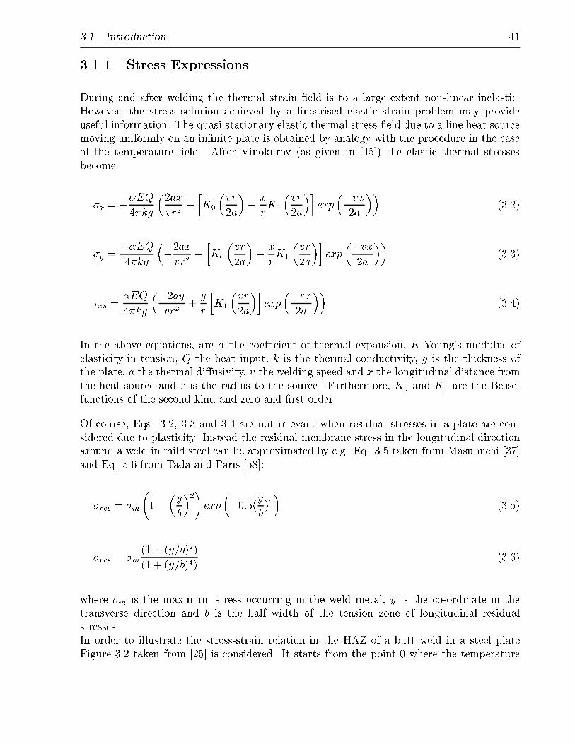
3.1. Introduction 41
3.1.1 Stress Expressions
During and after welding the thermal strain �eld is to a large extent non-linear inelastic.However, the stress solution achieved by a linearised elastic strain problem may provideuseful information. The quasi-stationary elastic thermal stress �eld due to a line heat sourcemoving uniformly on an in�nite plate is obtained by analogy with the procedure in the caseof the temperature �eld. After Vinokurov (as given in [45]) the elastic thermal stressesbecome
�x = ��EQ4�kg
�2ax
vr2+�K0
�vr
2a
�� x
rK1
�vr
2a
��exp
��vx2a
��(3.2)
�y =��EQ4�kg
��2axvr2
+�K0
�vr
2a
�+x
rK1
�vr
2a
��exp
��vx2a
��(3.3)
�xy =�EQ
4�kg
��2ayvr2
+y
r
�K1
�vr
2a
��exp
��vx2a
��(3.4)
In the above equations, are � the coe�cient of thermal expansion, E Young's modulus ofelasticity in tension, Q the heat input, k is the thermal conductivity, g is the thickness ofthe plate, a the thermal di�usivity, v the welding speed and x the longitudinal distance fromthe heat source and r is the radius to the source. Furthermore, K0 and K1 are the Besselfunctions of the second kind and zero and �rst order.
Of course, Eqs. 3.2, 3.3 and 3.4 are not relevant when residual stresses in a plate are con-sidered due to plasticity. Instead the residual membrane stress in the longitudinal directionaround a weld in mild steel can be approximated by e.g. Eq. 3.5 taken from Masubuchi [37]and Eq. 3.6 from Tada and Paris [58]:
�res = �m
1�
�y
b
�2!exp
��0:5(y
b)2�
(3.5)
�res = �m(1� (y=b)2)
(1 + (y=b)4)(3.6)
where �m is the maximum stress occurring in the weld metal, y is the co-ordinate in thetransverse direction and b is the half width of the tension zone of longitudinal residualstresses.In order to illustrate the stress-strain relation in the HAZ of a butt weld in a steel plateFigure 3.2 taken from [25] is considered. It starts from the point 0 where the temperature
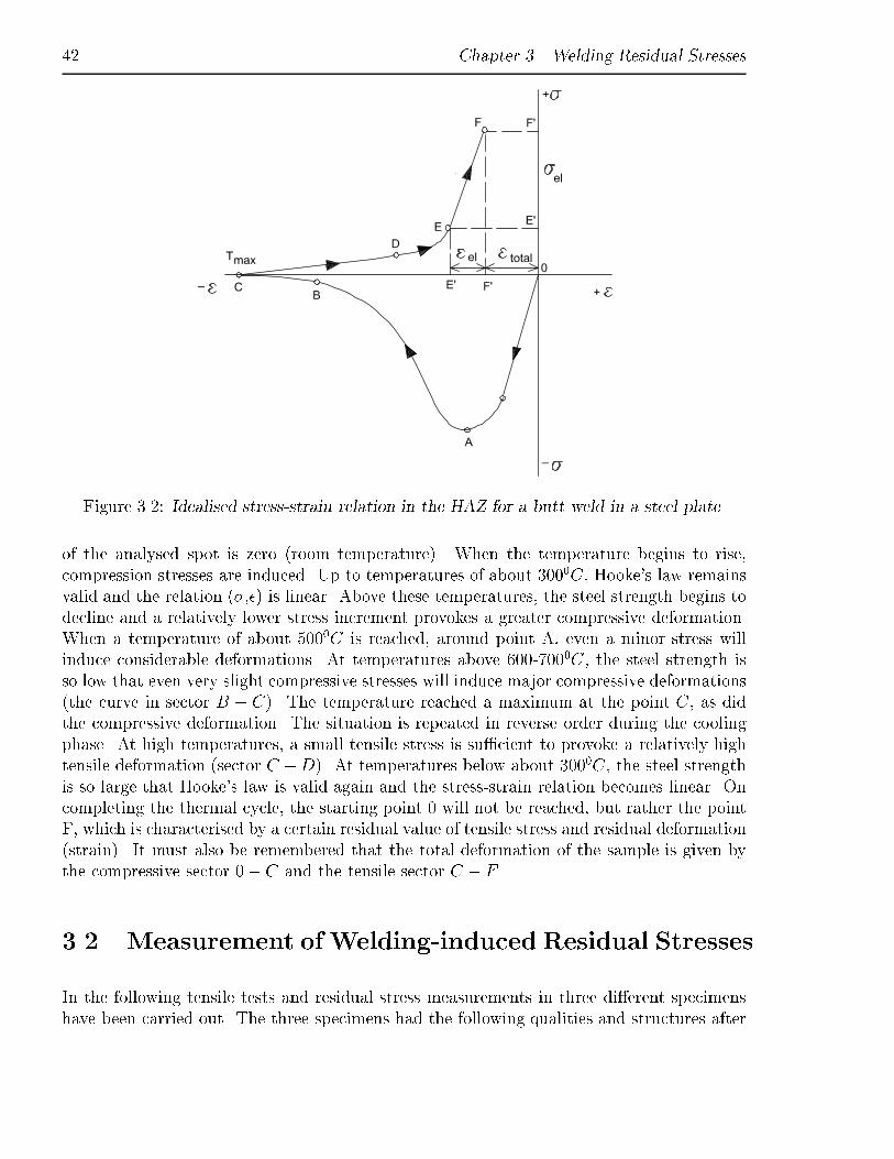
42 Chapter 3. Welding Residual Stresses
Figure 3.2: Idealised stress-strain relation in the HAZ for a butt weld in a steel plate.
of the analysed spot is zero (room temperature). When the temperature begins to rise,compression stresses are induced. Up to temperatures of about 3000C, Hooke's law remainsvalid and the relation (�,�) is linear. Above these temperatures, the steel strength begins todecline and a relatively lower stress increment provokes a greater compressive deformation.When a temperature of about 5000C is reached, around point A, even a minor stress willinduce considerable deformations. At temperatures above 600-7000C, the steel strength isso low that even very slight compressive stresses will induce major compressive deformations(the curve in sector B � C). The temperature reached a maximum at the point C, as didthe compressive deformation. The situation is repeated in reverse order during the coolingphase. At high temperatures, a small tensile stress is su�cient to provoke a relatively hightensile deformation (sector C �D). At temperatures below about 3000C, the steel strengthis so large that Hooke's law is valid again and the stress-strain relation becomes linear. Oncompleting the thermal cycle, the starting point 0 will not be reached, but rather the pointF, which is characterised by a certain residual value of tensile stress and residual deformation(strain). It must also be remembered that the total deformation of the sample is given bythe compressive sector 0� C and the tensile sector C � F .
3.2 Measurement of Welding-induced Residual Stresses
In the following tensile tests and residual stress measurements in three di�erent specimenshave been carried out. The three specimens had the following qualities and structures after
3.2. Measurement of Welding-induced Residual Stresses 43
the thermal rolling process: SS400 (which has a ferrite + pearlite microstructure), low carbon(bainite) and 9 % Ni (martensite).X-ray measurements have been made in order to determine the stress level in the as-rolledplate. After welding the sectioning method is used, based on measuring the stress relaxationby cutting the specimen into small parts vertical to the surface plane.
3.2.1 Tensile Test
In order to see if the rolling direction in uences the material strength and can be consideredas isotropic, tensile tests have been carried out for the three di�erent steel qualities. Thetensile test specimens are taken from three di�erent angles compared to the direction ofrolling. The angles are 00, 450 and 900.
The chemical composition for the steel used in these experiments is shown in Table 3.1.
Table 3.1: Main chemical compositions.
Type C Si Mn Ni NbSS400 0,16 0,22 0,82 ��� ���LCB 0,016 0,32 1,61 0,24 ���9%Ni 0,05 0,26 0,64 9,32 ���
The experiments were carried out at the Kawasaki Steel Corporation Research Center inMizushima, Japan. The tensile test machine is connected to a data receiver, which calculatesthe stresses and draws the "work curve". The machine has a maximum pull of 50kN andthe rate used in the experiments is 20N/(mm2 s), which is equivalent to a pulling speed of10mm/min. The specimens are standard circular specimens with a diameter of 6.00mm +/-0.03mm and a length of 100mm.
SS400 Steel
The results recorded for the SS400 steel are shown in the Table 3.2. The yield and tensilestrengths are approximately the same for the three directions. This is due to the �nishingrolling temperature which is rather high. The stress-strain curves show that the upper yieldlimit is approximately 276 MPa and the lower yield limit 268 MPa. Yielding occurs afterapproximately 1.7% of the total strain.
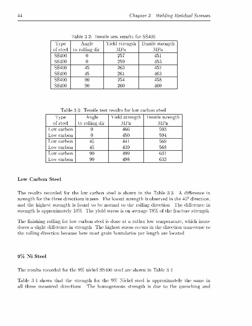
44 Chapter 3. Welding Residual Stresses
Table 3.2: Tensile test results for SS400.
Type Angle Yield strength Tensile strengthof steel to rolling dir. MPa MPaSS400 0 257 451SS400 0 259 453SS400 45 263 452SS400 45 261 463SS400 90 254 458SS400 90 260 460
Table 3.3: Tensile test results for low carbon steel.
Type Angle Yield strength Tensile strengthof steel to rolling dir. MPa MPa
Low carbon 0 466 593Low carbon 0 450 594Low carbon 45 441 569Low carbon 45 439 568Low carbon 90 499 631Low carbon 90 498 633
Low Carbon Steel
The results recorded for the low carbon steel is shown in the Table 3.3. A di�erence instrength for the three directions is seen. The lowest strength is observed in the 450 direction,and the highest strength is found to be normal to the rolling direction. The di�erence instrength is approximately 10%. The yield stress is on average 78% of the fracture strength.
The �nishing rolling for low carbon steel is done at a rather low temperature, which intro-duces a slight di�erence in strength. The highest stress occurs in the direction transverse tothe rolling direction because here most grain boundaries per length are located.
9% Ni Steel
The results recorded for the 9% nickel SS400 steel are shown in Table 3.4.
Table 3.4 shows that the strength for the 9% Nickel steel is approximately the same inall three measured directions. The homogeneous strength is due to the quenching and

3.2. Measurement of Welding-induced Residual Stresses 45
Table 3.4: Tensile test results for 9% Ni steel.
Type Angle Yield strength Tensile strengthof steel to rolling dir. MPa MPa9%Ni 0 583 7169%Ni 0 583 7179%Ni 45 585 7149%Ni 45 586 7149%Ni 90 589 7169%Ni 90 586 714
tempering process to which this type of plate has been exposed. These processes will cancelthe di�erences of strength introduced by the rolling process. The yield stress is of averageapproximately 82% of the tensile strength.
Summary
This study has shown that the posttreatment of steel and rolling at high temperature givesa very homogeneous strength in all directions. The maximum variation in strength was 10%found in the bainite steel with low carbon content, so the conclusion is that a rolled materialcan be assumed as isotropic. In general, the highest strength is in the direction normal tothe rolling direction.
3.2.2 X-ray Readings
The X-ray method can be used to measure residual stresses or, more precisely, strains dueto residual stresses. The X-ray technique is valid only for stress measurements in materialwhich is elastic, homogeneous and isotropic. The angle for the re ection of X-rays fromthe planes of the atoms (�) is sensitive to all factors that in uences the interplanar spacingof the re ecting planes. Since stresses within the elastic range can alter the spacing ofre ecting planes, enough to change the angle � in the Bragg's law by a measurable amount,the magnitude of stresses that are altering the normal spacing of the planes can be deducedfrom the observed 2� angles. Only elastic strains are indicated by the change in 2�. Thestrain can only be measured on the surface where the stress is relieved in the direction normalto the surface by lack of constraint in this direction. The interplanar spacing becomes a gaugelength which is altered proportionately by elastic stresses. A more profound description ofthe method is given in e.g. [10], [24] and [42].
As an illustration of the re ection or di�raction suppose that a monochromatic plane wave isintroduced to the atomic planes in the direction AB, as shown in Figure 3.3. The re ected

46 Chapter 3. Welding Residual Stresses
beams from successive parallel planes of atoms are reinforced in one direction BC; thedi�raction direction.
Figure 3.3: Di�raction resulting from re ection from adjacent atomic planes of a monochro-matic plane wave.
Bragg's law, Eq. 3.7, de�nes the condition for di�raction as follows:
n� = 2dsin� (3.7)
where n is the number of wavelength di�erence in the path for waves for successive planes, �is the wavelength, d is the interatomic spacing and � is the angle between the incident beamand the planes of the atoms. Eq. 3.7 shows that if the wavelength of the X-ray is known, theinterplanar spacing d can be determined by measuring the angle �. Before starting weldingon the 600 V-groove by multipass SAW the homogeneity "stress level" is investigated byX-ray. The X-ray results for the present three specimens before welding are presented inFigure 3.4.
The results should not be regarded as absolute values, but more as an indicator of thehomogeneity of the inherent stress level brought about by the rolling process. A somewhatnon-uniform stress level is seen, especially for the SS400 steel. The stresses measured aresurface stresses, which here are negatives, but in the middle of the plate the stresses mightbee positive, i.e. in tension.
3.2.3 Welding Experiments
The used welding method is submerged arc welding (SAW). The weld joint is a 600 V-groove.The �ve beads are laid down by a "Bugo-tractor". All the plates have the welding parametersshown in Table 3.5.
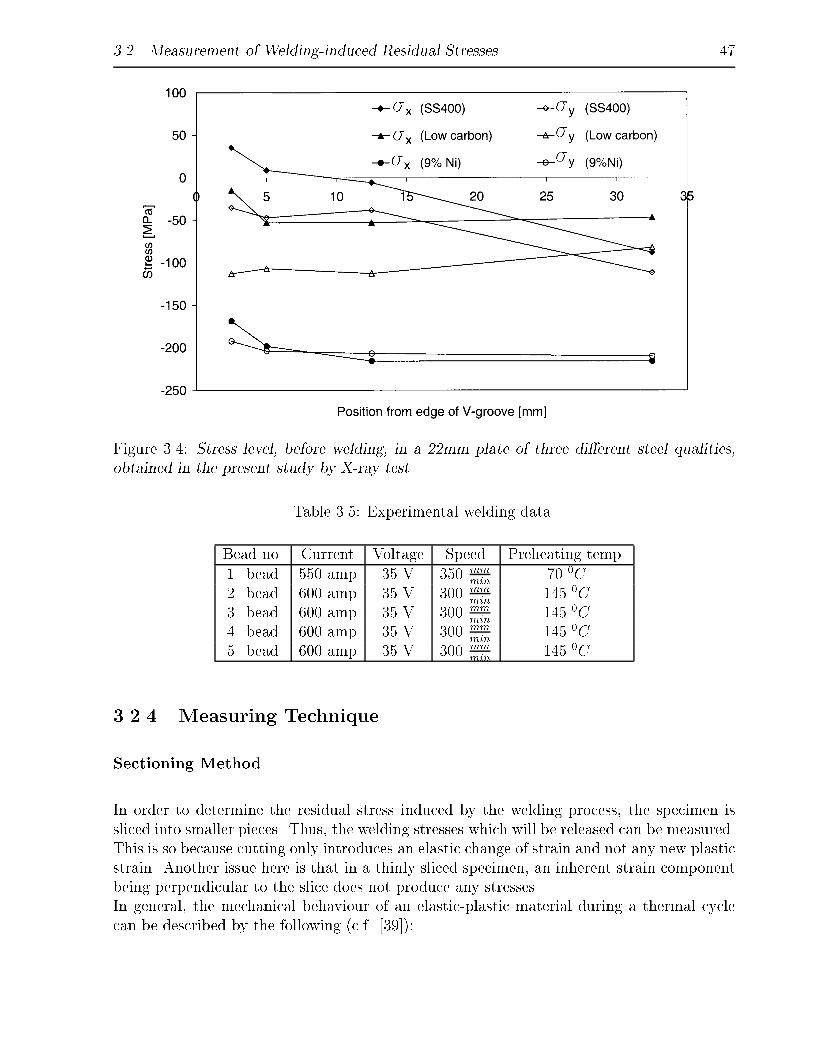
3.2. Measurement of Welding-induced Residual Stresses 47
Figure 3.4: Stress level, before welding, in a 22mm plate of three di�erent steel qualities,obtained in the present study by X-ray test.
Table 3.5: Experimental welding data.
Bead no. Current Voltage Speed Preheating temp.1. bead 550 amp 35 V 350 mm
min70 0C
2. bead 600 amp 35 V 300 mmmin
145 0C3. bead 600 amp 35 V 300 mm
min145 0C
4. bead 600 amp 35 V 300 mmmin
145 0C5. bead 600 amp 35 V 300 mm
min145 0C
3.2.4 Measuring Technique
Sectioning Method
In order to determine the residual stress induced by the welding process, the specimen issliced into smaller pieces. Thus, the welding stresses which will be released can be measured.This is so because cutting only introduces an elastic change of strain and not any new plasticstrain. Another issue here is that in a thinly sliced specimen, an inherent strain componentbeing perpendicular to the slice does not produce any stresses.In general, the mechanical behaviour of an elastic-plastic material during a thermal cyclecan be described by the following (c.f. [39]):
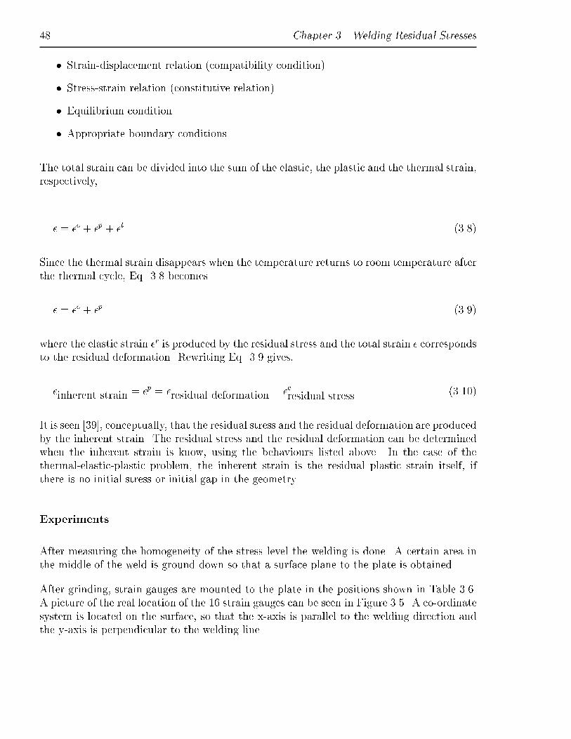
48 Chapter 3. Welding Residual Stresses
� Strain-displacement relation (compatibility condition)
� Stress-strain relation (constitutive relation)
� Equilibrium condition
� Appropriate boundary conditions
The total strain can be divided into the sum of the elastic, the plastic and the thermal strain,respectively,
� = �e + �p + �t (3.8)
Since the thermal strain disappears when the temperature returns to room temperature afterthe thermal cycle, Eq. 3.8 becomes
� = �e + �p (3.9)
where the elastic strain �e is produced by the residual stress and the total strain � correspondsto the residual deformation. Rewriting Eq. 3.9 gives,
�inherent strain = �p = �residual deformation � �eresidual stress (3.10)
It is seen [39], conceptually, that the residual stress and the residual deformation are producedby the inherent strain. The residual stress and the residual deformation can be determinedwhen the inherent strain is know, using the behaviours listed above. In the case of thethermal-elastic-plastic problem, the inherent strain is the residual plastic strain itself, ifthere is no initial stress or initial gap in the geometry.
Experiments
After measuring the homogeneity of the stress level the welding is done. A certain area inthe middle of the weld is ground down so that a surface plane to the plate is obtained.
After grinding, strain gauges are mounted to the plate in the positions shown in Table 3.6.A picture of the real location of the 16 strain gauges can be seen in Figure 3.5. A co-ordinatesystem is located on the surface, so that the x-axis is parallel to the welding direction andthe y-axis is perpendicular to the welding line.
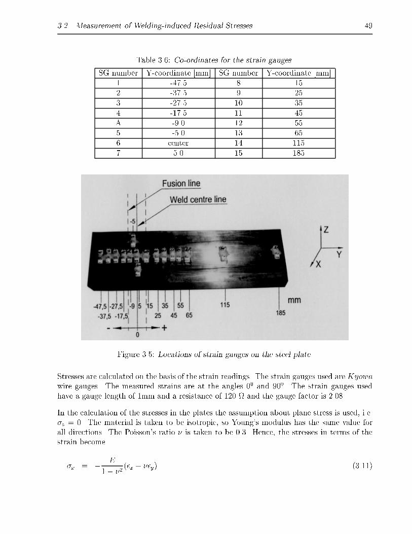
3.2. Measurement of Welding-induced Residual Stresses 49
Table 3.6: Co-ordinates for the strain gauges.
SG number Y-coordinate [mm] SG number Y-coordinate [mm]1 -47.5 8 152 -37.5 9 253 -27.5 10 354 -17.5 11 45A -9.0 12 555 -5.0 13 656 center 14 1157 5.0 15 185
Figure 3.5: Locations of strain gauges on the steel plate.
Stresses are calculated on the basis of the strain readings. The strain gauges used are Kyowawire gauges. The measured strains are at the angles 00 and 900. The strain gauges usedhave a gauge length of 1mm and a resistance of 120 and the gauge factor is 2.08.
In the calculation of the stresses in the plates the assumption about plane stress is used, i.e.�z = 0. The material is taken to be isotropic, so Young's modulus has the same value forall directions. The Poisson's ratio � is taken to be 0.3. Hence, the stresses in terms of thestrain become
�x = � E
1� �2(�x + ��y) (3.11)
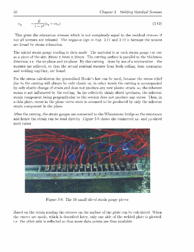
50 Chapter 3. Welding Residual Stresses
�y = � E
1� �2(�y + ��x) (3.12)
This gives the relaxation stresses which is not completely equal to the residual stresses ifnot all stresses are released. The negative sign in Eqs. 3.11 and 3.12 is because the strainsare found by strain relaxation.
The initial strain gauge reading is then made. The material is at each strain gauge cut outas a piece of the size 20mm x 8mm x 20mm. The cutting surface is parallel to the thicknessdirection, i.e. the xz-plane and yz-plane. By this cutting { done by use of a microcutter { thestresses are relieved, so that the actual residual stresses from both rolling, heat treatmentand welding together, are found.
For the stress calculation the generalised Hooke's law can be used, because the stress reliefdue to the cutting will always be only elastic or, in other words the cutting is accompaniedby only elastic change of strain and does not produce any new plastic strain, so, the inherentstrain is not in uenced by the cutting. In the relatively thinly sliced specimen, the inherentstrain component being perpendicular to the section does not produce any stress. Thus, ina thin plate, stress in the plane stress state is assumed to be produced by only the inherentstrain component in the plane.
After the cutting, the strain gauges are connected to the Wheatstone bridge so the resistanceand hence the strain can be read directly. Figure 3.6 shows the connected xz- and yz-slicedsteel cubes.
Figure 3.6: The 16 small sliced strain gauge pieces.
Based on the strain reading the stresses on the surface of the plate can be calculated. Whenthe curves are made, which is described later, only one side of the welded plate is plotted,i.e. the other side is re ected so that more data points are thus available.
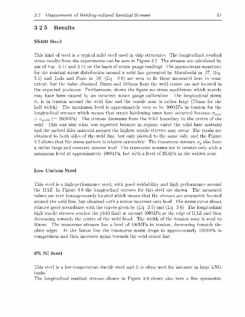
3.2. Measurement of Welding-induced Residual Stresses 51
3.2.5 Results
SS400 Steel
This kind of steel is a typical mild steel used in ship structures. The longitudinal residualstress results from the experiments can be seen in Figure 3.7. The stresses are calculated byuse of Eqs. 3.11 and 3.12 on the basis of strain gauge readings. The approximate equationsfor the residual stress distribution around a weld line presented by Masubuchi in [37] (Eq.3.5) and Tada and Paris in [58] (Eq. 3.6) are seen to �t those measured here to someextent, but the value obtained 45mm and 185mm from the weld centre are not located inthe expected positions. Furthermore, shows the �gure no stress equlibrium which mainlymay have been caused by an incorrect strain gauge calibration. The longitudinal stress�x is in tension around the weld line and the tensile zone is rather large (75mm for thehalf width). The maximum level is approximately seen to be 300MPa in tension for thelongitudinal stresses which means that strain hardening must have occurred because �max
> �yield (= 260MPa). The stresses decreases from the HAZ boundary to the centre of theweld. This was also what was expected because in regions where the solid base materialand the melted �ller material merged the highest tensile stresses may occur. The strain areobtained to both sides of the weld line, but only plotted to the same side, and the Figure3.7 shows that the stress pattern is relative symmetric. The transverse stresses �y also havea rather large and constant tension level. The transverse stresses are in tension only with amaximum level at approximately 100MPa, but with a level of 25MPa in the welded zone.
Low Carbon Steel
This steel is a high-performance steel, with good weldability and high performance aroundthe HAZ. In Figure 3.8 the longitudinal stresses for this steel are shown. The measuredvalues are very homogeneously located which means that the stresses are symmetric locatedaround the weld line, but obtained with a minor incorrect zero level. The stress curve showsrelative good accordance with the curves given by (Eq. 3.5) and (Eq. 3.6). The longitudinalhigh tensile stresses reaches the yield limit at around 500MPa at the edge of HAZ and thendecreasing towards the centre of the weld bead. The width of the tension zone is read to90mm. The transverse stresses has a level of 100MPa in tension, decreasing towards theplate edges. At the fusion line the transverse stress drops to approximately 100MPa incompression and then increases again towards the weld centre line.
9% Ni Steel
This steel is a low-temperature ductile steel and it is often used for instance in large LNGtanks.The longitudinal residual stresses shown in Figure 3.9 shows also here a �ne symmetric
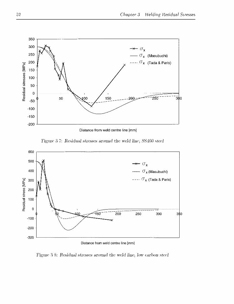
52 Chapter 3. Welding Residual Stresses
Figure 3.7: Residual stresses around the weld line, SS400 steel.
Figure 3.8: Residual stresses around the weld line, low carbon steel.
3.2. Measurement of Welding-induced Residual Stresses 53
stress pro�le, although the zero level is not located properly in order to obtained stressequlibrium, but this "error" may be due to the strain gauge calibration. The agreementbetween the measured values and those given by (Eq. 3.5) and (Eq. 3.6) is not good. Thiswas expected because the given equations are made as assumtions for longitudinal residualstress distribution in mild steel. The longitudinal stresses decrease steeply in the HAZ and isdisplaced into the compression range. In the weld centre the stresses are reversed into a lowtension. The peak for �x is around 400MPa measured 17.5mm from the weld centre which ismuch below the yield limit. From the middle of the plate half the stresses reversal into thetension range and the stresses keeps in tension towards the plate edge. This may occur as aconsequence of complex formation mechanism of residual stresses which is not dealt with inthe present study. The width of the tension zone is read to 100mm. The transverse stressesare nearly only in tension at a level of approximately 50MPa outside the HAZ.
Figure 3.9: Residual stresses around the weld line, 9%Ni steel.
Summary
Table 3.7 summarises the main results obtained in the experiments. The maximum stressesrange from 350MPa to 500MPa, and the width of the tension zone of the residual stressesranges from 90 to 150mm for the butt welds in these 20mm steel plates. The width of thetension zone can be discussed because it is measured by use of the stress �gures, whichincludes a levelling incorrectness. Di�erence in the stress distribution in the HAZ for mildsteel and high tensile steel is what was seen in [45].

54 Chapter 3. Welding Residual Stresses
Table 3.7: Summary of the results of the longitudinal residual stress measurements.
Type of steel Joint type Max. stress Width of tension zoneSS400 Butt joint, 5 beads 350 MPa 150mmLow C Butt joint, 5 beads 500 MPa 90mm9%Ni Butt joint, 5 beads 400 MPa 100mm
Uncertainties
The assumption about plane stress in a 20mm x 8mm x 20mm small steel piece may not beas good as we would like it to be.
When measuring the strain in the x; y-plane it is assumed that the stress state is plane. Forthe whole plate before cutting, this assumption is rather accurate because of the extension ofthe plate in the x; y-direction compared to the relatively thin z-direction (400x400x20mm).After cutting the gauges out in small cubes the situation is another. The cubes are 20mmin length, 8mm in width and 20mm in depth. Here the assumption about plane stress is lessgood. Of course, it is not technically possible to cut the cubes in the same x/z- or y/z-ratioas for the whole plate, but a small comparative study has been made for two sizes of "gaugecubes": 20mm x 8mm x 20mm and 20mm x 8mm x 3mm, as illustrated in Figure 3.10.
Figure 3.10: Sectioning of the 20mm thick block into a 3mm thick block mounted with astrain gauge.
From Figure 3.11 it is seen that the thickness of the slice in uences the gauged stresses.The thin slice gives in general lower stresses than the thick slice. The values for �y 12.5mmand 35mm away from the weld line do not match each other so well as the other obtainedstresses, this can be due to technical errors with the strain gauges, but the same tendencywith lower stresses for the thin sliced specimens is seen.
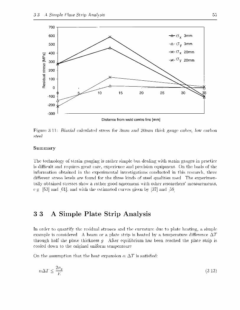
3.3. A Simple Plate Strip Analysis 55
Figure 3.11: Biaxial calculated stress for 3mm and 20mm thick gauge cubes, low carbonsteel.
Summary
The technology of strain gauging is rather simple but dealing with strain gauges in practiceis di�cult and requires great care, experience and precision equipment. On the basis of theinformation obtained in the experimental investigations conducted in this research, threedi�erent stress levels are found for the three kinds of steel qualities used. The experimen-tally obtained stresses show a rather good agreement with other researchers' measurements,e.g. [53] and [61], and with the estimated curves given by [37] and [58].
3.3 A Simple Plate Strip Analysis
In order to quantify the residual stresses and the curvature due to plate heating, a simpleexample is considered. A beam or a plate strip is heated by a temperature di�erence �Tthrough half the plate thickness g. After equilibrium has been reached the plate strip iscooled down to the original uniform temperature.
On the assumption that the heat expansion � �T is satis�ed:
��T � 2�yE
(3.13)
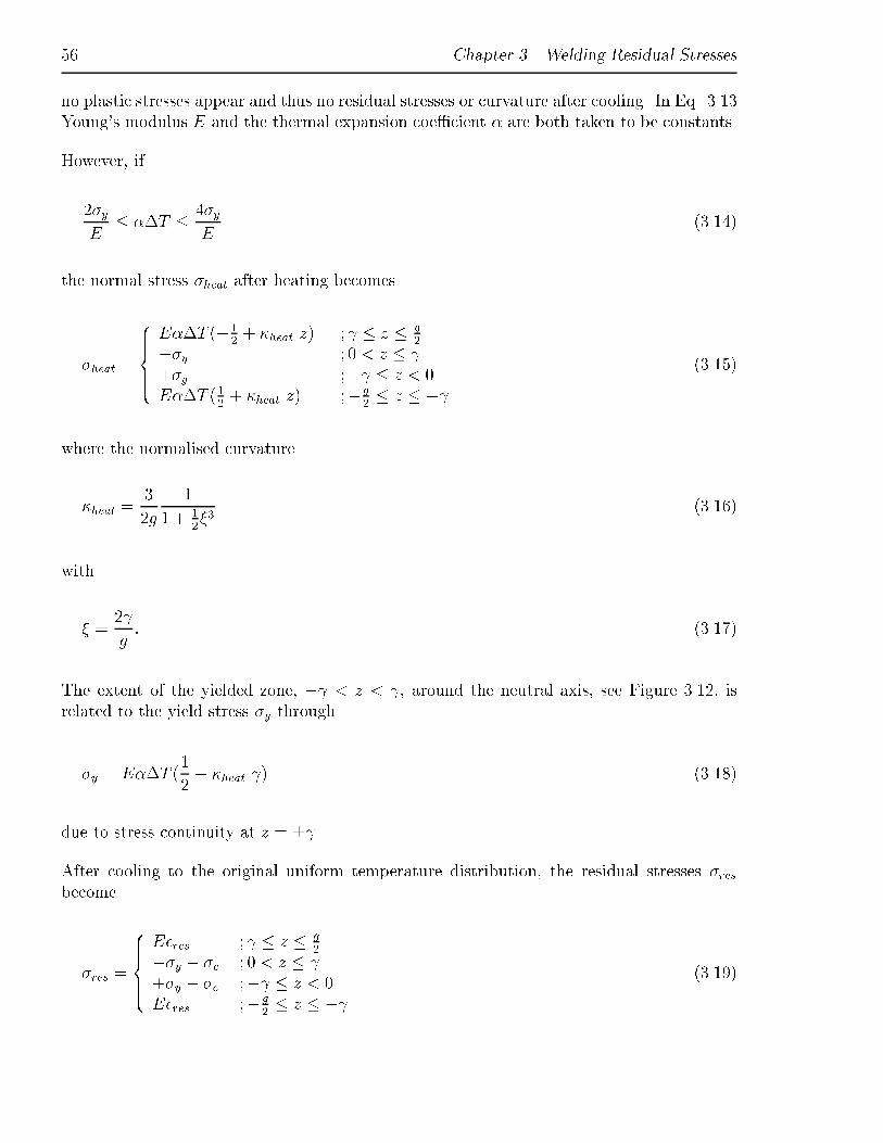
56 Chapter 3. Welding Residual Stresses
no plastic stresses appear and thus no residual stresses or curvature after cooling. In Eq. 3.13Young's modulus E and the thermal expansion coe�cient � are both taken to be constants.
However, if
2�yE
� ��T � 4�yE
(3.14)
the normal stress �heat after heating becomes
�heat =
8>>><>>>:
E��T (�12+ �heat z) ; � z � g
2
��y ; 0 < z � +�y ;� � z < 0E��T (1
2+ �heat z) ;�g
2� z � �
(3.15)
where the normalised curvature
�heat =3
2g
1
1 + 12�3
(3.16)
with
� =2
g: (3.17)
The extent of the yielded zone, � < z < , around the neutral axis, see Figure 3.12, isrelated to the yield stress �y through
�y = E��T (1
2� �heat ) (3.18)
due to stress continuity at z = � .
After cooling to the original uniform temperature distribution, the residual stresses �resbecome
�res =
8>>><>>>:
E�res ; � z � g2
��y � �e ; 0 < z � +�y � �e ;� � z < 0E�res ;�g
2� z � �
(3.19)
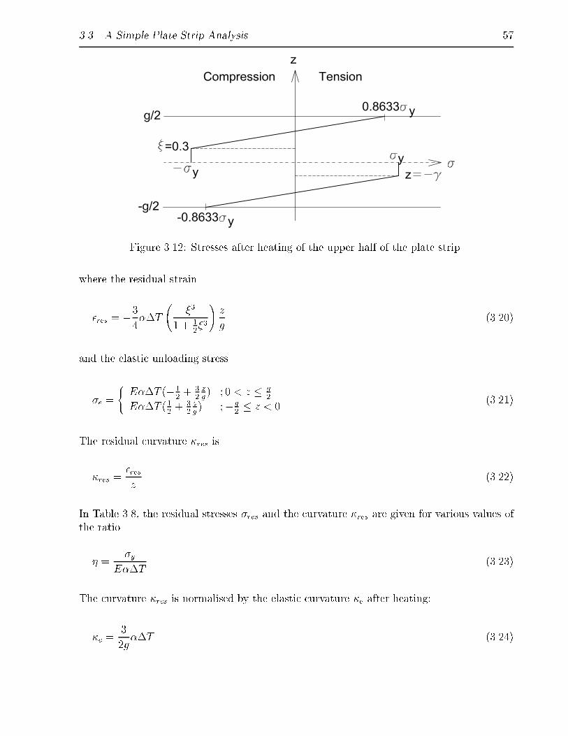
3.3. A Simple Plate Strip Analysis 57
Figure 3.12: Stresses after heating of the upper half of the plate strip.
where the residual strain
�res = �34��T
�3
1 + 12�3
!z
g(3.20)
and the elastic unloading stress
�e =
(E��T (�1
2+ 3
2zg) ; 0 < z � g
2
E��T (12+ 3
2zg) ;�g
2� z < 0
(3.21)
The residual curvature �res is
�res =�resz
(3.22)
In Table 3.8, the residual stresses �res and the curvature �res are given for various values ofthe ratio
� =�y
E��T(3.23)
The curvature �res is normalised by the elastic curvature �e after heating:
�e =3
2g��T (3.24)
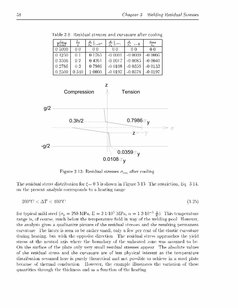
58 Chapter 3. Welding Residual Stresses
Table 3.8: Residual stresses and curvature after cooling.�y
E��T2 g
��yjz=0+ �
�yjz= �
�y
���z= g
2
�res�e
0.5000 0.0 0.0 0.0 0.0 0.00.4250 0.1 0.1765 -0.0001 -0.0009 -0.00050.3506 0.2 0.4261 -0.0017 -0.0085 -0.00400.2786 0.3 0.7986 -0.0108 -0.0359 -0.01330.2500 0.340 1.0000 -0.0197 -0.0578 -0.0197
Figure 3.13: Residual stresses �res after cooling.
The residual stress distribution for �= 0.3 is shown in Figure 3.13. The restriction, Eq. 3.14,on the present analysis corresponds to a heating range
200oC < �T < 400oC (3.25)
for typical mild steel (�y = 250 MPa, E = 2.1�105 MPa, � = 1.2�10�5 1K). This temperature
range is, of course, much below the temperature �eld in way of the welding pool. However,the analysis gives a qualitative picture of the residual stresses and the resulting permanentcurvature. The latter is seen to be rather small, only a few per cent of the elastic curvatureduring heating, but with the opposite direction. The residual stress approaches the yieldstress at the neutral axis where the boundary of the unheated zone was assumed to be.On the surface of the plate only very small residual stresses appear. The absolute valuesof the residual stress and the curvature are of less physical interest as the temperaturedistribution assumed here is purely theoretical and not possible to achieve in a steel platebecause of thermal conduction. However, the example illustrates the variation of thesequantities through the thickness and as a function of the heating.
Chapter 4
Welding Distortion Measurements
4.1 Introduction
A serious problem in ship building is the distortion introduced by the welding. A number ofstudies have been performed on the calculation of residual stresses and deformations, but feware useful in the design process. Most of these calculation methods are either rather restrictedand made for special purposes, e.g. Hansen [22] or Malisius [34], or too complicated to beused in design and production, e.g. Okerblom [41]. Most of the formulas are semi-empiricaland based on measurements of deformations and strains and cannot take into account whatreally happens in the heat-a�ected zone (HAZ) when the welding is cooling down.
In the past, attempts were made to investigate changes in the bending deformation due tovarying pertinent parameters, see e.g. Iwamura [26] and Masubuchi [35]. These investiga-tions cover many practical aspects of the process, but are based mainly on experimentaldata.
In welding of plates, plastic deformations are created as a result of the heating, melting andcooling processes. The stress-strain behaviour of the plate during welding is complex andtherefore the in-plane and lateral de ections after the welding are di�cult to predict. Themost signi�cant factors a�ecting the inherent de ections are
� Heat input rate and distribution
� Constraints of the plate (boundary conditions)
� Initial curvature
� Residual stresses in the plate due to rolling

60 Chapter 4. Welding Distortion Measurements
The purpose of this chapter is to investigate the deformation due to the welding process.These deformations are obtained from measurements on T-beams from the productions and�llet and butt welds in model size. The constraints, which are �xed along one of the sideedges of the plates, are kept equal in all model welding cases.
The T-beams dealt with in this chapter are so-called "fabricated built-up beams", [28].The most critical deformation in a relatively long and slender beam is from a productionpoint of view the uneven longitudinal deformation. For straightening of the deformation,heating of web plates is necessary. To manufacture built-up beams automatically, controlof deformations is needed, on the basis of precise estimation of longitudinal deformationsdue to welding and heating. Built-up T-beams are normally manufactured by Odense SteelShipyard itself. The plastic strains are caused by the uneven temperature distribution aroundweld beads and the restraining e�ect of the section.
At Odense Steel Shipyard Ltd, measurements have been carried out in the assembly hallsand in the welding laboratory.
Attention has been paid to
1. Longitudinal shrinkage
2. Transverse shrinkage
3. De ections
4. Welding-induced strain
The measurements have been concentrated on butt and �llet welds, with most weight to�llets.
In a previous study made by Rasmussen [46] the shrinkage of T-beams produced at OdenseSteel Shipyard was measured. The results are shown in Table 4.1. The welding parametersfor the T-beams are
Speci�ed A-measure = 3.5mm.Current = 750 � 50 ampVoltage = 28 � 2 VTorch velocity = 150 � 10 cm
min
Wire diameter = 2 x 2mm
In Table 4.1 are the longitudinals marked with a s for the starboard side and a p for portside.
The face plate has a dimension of 150 x 25mm except for PD 083s, 181s, 180s, 214s, 215s,216s and 217s, which have a face dimension of 130 x 16mm.

4.1. Introduction 61
Table 4.1: Longitudinal shrinkage of the body of T-beams (longitudinals).
PD number Dim. of web Length before [mm] Length after [mm] Shrinkage [mm]
081s 400 x 11 13867 13863 4083s 380 x 11 13669 13858 11356s 420 x 11 13055 13054 1357s 420 x 11 13057 13052 5181s 300 x 11 14375 14369 6180s 300 x 11 14373 14368 5177s 300 x 11 14374 14374 0176s 300 x 11 14374 14372 2173s 400 x 11 14374 14369 5199s 300 x 11 14376 14375 1200s 300 x 11 14375 14370 5214s 300 x 11 14375 14368 7215s 300 x 11 14375 14368 7216s 260 x 11 14375 14367 8217s 260 x 11 14375 14368 7219s 300 x 11 13068 13057 1224s 400 x 11 13058 13053 5115p 380 x 11 13064 13060 4116p 380 x 11 13063 13057 6218p 300 x 11 13060 13057 3219p 300 x 11 13060 13057 3218s 300 x 11 13058 13056 2111p 380 x 11 13061 13055 6346s 400 x 11 13060 13053 7347s 400 x 11 13059 13055 4302s 420 x 11 13058 13052 6301s 420 x 11 13058 13052 6351s 480 x 11 13058 13051 7172p 400 x 11 14376 14372 4173p 400 x 11 14375 14369 6176p 300 x 11 14374 14373 1177p 300 x 11 14374 14372 2
Statistics Mean value 4.59Std. deviation 2.46

62 Chapter 4. Welding Distortion Measurements
PD 356s, 357s, 346s, 347s, 302s, 301s, 351s have a dimension of 200 x 25mm for the faceplate.
If it is assumed that the shrinkage of a 13720mm longitudinal is a superposition of e.g. 34400mm long T-pro�les, then the shrinkage for one 400mm T-pro�le should be approximately0.134mm (0.335mm/m) with a standard deviation of about 50%. The model size T-pro�leswelded in the laboratory, (see later), have on average a longitudinal shrinkage of -0.13mm i.e.an extension for the pro�les without forced cooling and approximately 0.27 i.e. a shrinkagefor the pro�les with forced cooling. This indicates that the boundary conditions need to beright in the sense of cooling or more correct heat absorption. It is a coincidence that thenumerical value of the shrinkage is the same.
4.2 Analysis of the Shrinkage in Test Models
4.2.1 Fillets
The test pieces of �llet welds have the dimensions 400mm x 300mm for the ange plate and400mm x 150mm for the web plate. The thickness is 12mm for both plates.
A table with three support legs and �xtures for dial indicators was used, see Figure 4.1.In order to let the plate be free to de ect, so that the angular change could be obtained asfunction of time, a �xture board with a heavy �x plate clamping the plate was used, seeFigure 4.2. As also illustrated by Figure 4.2, a robot was used in order to get the most
Figure 4.1: The �xture board, with threesupports and pins for dialindicators.
Figure 4.2: A T-pro�le clamped by the �x-ture.
homogeneous welding.
The de ection of the T-pro�le, Figure 4.3, is measured continuously in time, e.g. during thewhole welding and cooling process. The used digital dial indicator is a TESER InstrumentDigico 10, connected to a PC data logger by an RS232 optic �bre cable.

4.2. Analysis of the Shrinkage in Test Models 63
Figure 4.3: Cross-section of the T-pro�le inthe �xture, without clamp plate.
Figure 4.4: The tool used for measuring therelatively small shrinkage values.
The longitudinal and transverse shrinkage are measured by use of a micrometer screw gaugeas shown in Figure 4.4. The strain readings are made by standard strain gauges fromHottinger Baldwin Messtechnik. The gauges are of the type 3/120 RE 21, rosette gauges.The positioning on the T-pro�le can be seen in Figure 4.5 and Figure 4.6. The gauge factoris 2.03.
Figure 4.5: The strain gauge locations on the"back"side of the T-pro�le.
Figure 4.6: The strain gauge locations on the"front" side of the T-pro�le.
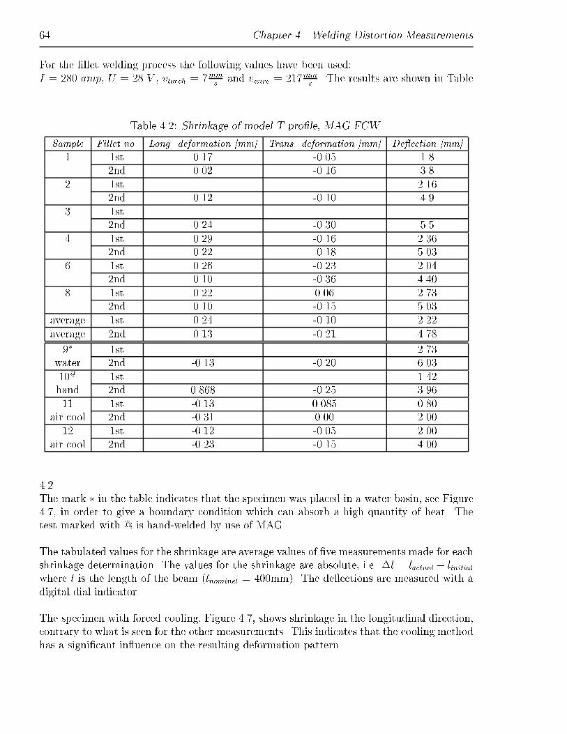
64 Chapter 4. Welding Distortion Measurements
For the �llet welding process the following values have been used:I = 280 amp, U = 28 V , vtorch = 7mm
sand vwire = 217mm
s. The results are shown in Table
Table 4.2: Shrinkage of model T-pro�le, MAG FCW.
Sample Fillet no. Long. deformation [mm] Trans. deformation [mm] De ection [mm]
1 1st 0.17 -0.05 1.82nd 0.02 -0.16 3.8
2 1st | | 2.162nd 0.12 -0.10 4.9
3 1st | | |2nd 0.24 -0.30 5.5
4 1st 0.29 -0.16 2.362nd 0.22 -0.18 5.03
6 1st 0.26 -0.23 2.042nd 0.10 -0.36 4.40
8 1st 0.22 0.06 2.732nd 0.10 -0.15 5.03
average 1st 0.24 -0.10 2.22average 2nd 0.13 -0.21 4.78
9� 1st | | 2.73water 2nd -0.13 -0.20 6.0310@ 1st | | 1.42hand 2nd 0.868 -0.25 3.9611 1st -0.13 0.085 0.80
air cool 2nd -0.31 0.00 2.0012 1st -0.12 -0.05 2.00
air cool 2nd -0.23 -0.15 4.00
4.2.The mark � in the table indicates that the specimen was placed in a water basin, see Figure4.7, in order to give a boundary condition which can absorb a high quantity of heat. Thetest marked with @ is hand-welded by use of MAG.
The tabulated values for the shrinkage are average values of �ve measurements made for eachshrinkage determination. The values for the shrinkage are absolute, i.e. �l = lactual � linitialwhere l is the length of the beam (lnominel = 400mm). The de ections are measured with adigital dial indicator.
The specimen with forced cooling, Figure 4.7, shows shrinkage in the longitudinal direction,contrary to what is seen for the other measurements. This indicates that the cooling methodhas a signi�cant in uence on the resulting deformation pattern.

4.2. Analysis of the Shrinkage in Test Models 65
Figure 4.7: T-specimen with prescribed cooling boundary condition.
Figure 4.8: Longitudinal shrinkage for the forced air-cooled T-pro�le, sample 11.
Two T-pro�les have been cooled with air (samples 11 & 12), and then measured for thereason of obtaining the shrinkage at �ve di�erent positions along the transverse edge of the ange plate. The longitudinal strain is depicted in Figure 4.8. As illustrated in the Figure4.8 the welding of the �rst �llet has almost the same e�ect for the shrinkage as the second�llet.The longitudinal strain is -0.00078 (approx. -0.31mm) along the bead adjacent to the centreline. The transverse shrinkage was also measured and the transverse strain was about -0.0003 (approx. 0.1mm) for the �nal �llet weld. The full size tests showed an averagelongitudinal shrinkage at 0.134mm, which is more than half the value for the forced air-
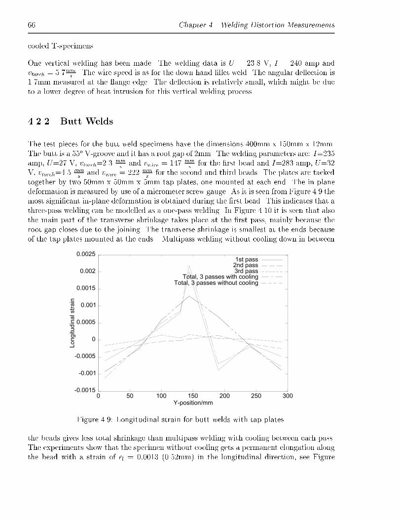
66 Chapter 4. Welding Distortion Measurements
cooled T-specimens.
One vertical welding has been made. The welding data is U = 23.8 V, I = 240 amp andvtorch = 5.7mm
s. The wire speed is as for the down hand �llet weld. The angular de ection is
1.7mm measured at the ange edge. The de ection is relatively small, which might be dueto a lower degree of heat intrusion for this vertical welding process.
4.2.2 Butt Welds
The test pieces for the butt weld specimens have the dimensions 400mm x 150mm x 12mm.The butt is a 55o V-groove and it has a root gap of 2mm. The welding parameters are: I=235amp, U=27 V, vtorch=2.3
mms
and vwire = 147 mms
for the �rst bead and I=283 amp, U=32V, vtorch=4.5
mms
and vwire = 222 mms
for the second and third beads. The plates are tackedtogether by two 50mm x 50mm x 5mm tap plates, one mounted at each end. The in-planedeformation is measured by use of a micrometer screw gauge. As it is seen from Figure 4.9 themost signi�cant in-plane deformation is obtained during the �rst bead. This indicates that athree-pass welding can be modelled as a one-pass welding. In Figure 4.10 it is seen that alsothe main part of the transverse shrinkage takes place at the �rst pass, mainly because theroot gap closes due to the joining. The transverse shrinkage is smallest at the ends becauseof the tap plates mounted at the ends. Multipass welding without cooling down in between
Figure 4.9: Longitudinal strain for butt welds with tap plates.
the beads gives less total shrinkage than multipass welding with cooling between each pass.The experiments show that the specimen without cooling gets a permanent elongation alongthe bead with a strain of �l = 0:0013 (0.52mm) in the longitudinal direction, see Figure

4.2. Analysis of the Shrinkage in Test Models 67
Figure 4.10: Transverse strain for butt welds with tap plates.
4.9. The transverse strain becomes �t = �0:0065 (approximately -2mm) for the specimenwithout cooling. The transverse shrinkage is largest in the middle of the plate, which maybe caused by the tap plates, see Figure 4.10.
A simple empirical expression for the transverse shrinkage st of a V-groove is given in Floor[15] as
st = 0:16 g tanV
2+ 0:4 G = 1:8 mm (4.1)
where g is the plate thickness, V is the groove angle and G is the gap. This simple formulathus shows good agreement with the present experiments with continous cooling, but itsgeneral validity is not known.
The transverse shrinkage during multipass welding (e.g. as shown in Figure 4.10) of con-strained butt-welded joints shows that the rate of shrinkage diminishes during later passes.This happens because the resistance of the previous welds to the thermal expansion of thebase metal increases as the weld becomes larger.
The experiments are rather simple, but the tendency is permanent elongation and shrinkagein the transverse direction for the butt weld for the used model size.
Out-of-plane measurements were made of the butt-welded test specimens, too. Figure 4.11shows the maximum out-of-plane deformation w along the longitudinal X-axis at three points

68 Chapter 4. Welding Distortion Measurements
Figure 4.11: Measured out-of-plane deformation for butt weld, max. angular de ection.
(middle and end points). It is seen from the �gure that the out-of-plane deformation issmallest in the middle, (x = 200mm).
The butt weld is built up of three beads. These beads are welded either continuously orwith cooling in between. In Table 4.3 the continuous welds are marked with �, and thecooled-down welds are marked with |. All measuring points are related to the centre line.The samples marked with 3 have three tack welds in the groove. The other samples arewelded with tab plates at the ends.

4.2. Analysis of the Shrinkage in Test Models 69
Table 4.3: Average shrinkage of butt welds close to the weld line, MAG FCW.
Sample Bead no. Long. deformation [mm] Trans. deformation [mm] De ection [mm]
1� 3rd 0.11 -2.32 1.752� 3rd 0.37 -2.31 1.003| 1st 0.33 -1.29 0.4
2nd 0.08 -1.8 1.083rd 0.05 -2.37 2.25
4| 1st 0.21 -0.23 0.502nd 0.14 -0.77 0.503rd 0.19 -1.22 1.77
53 | 1st 0.24 -1.66 1.82nd 0.31 -2.02 3.53rd 0.26 -2.59 6.0
63 | 1st 0.32 -1.14 0.752nd 0.32 -1.66 2.43rd 0.32 -2.21 4.35
73, � 3rd 0.24 -1.96 5.4average 3rd 0.22 -2.14 3.2
It is seen in Table 4.3 that the longitudinal deformation is positive, which means that theplate is elongated. This behaviour was also found in a study by Matting and Rubo, quotedin [34]. In their test a 200mm long V-groove was welded with electrodes in a 10mm thicksteel plate. The shrinkage obtained is illustrated in Figure 4.12.
Figure 4.13 shows shrinkage values obtained by the present experiments. The number ofpasses in uences the deformation. The tendency that the shrinkage increases when thenumber of beads increases as obtained by Matting and Rubo in Figure 4.12 is not seen here.The transverse shrinkage increases with the number of passes in both studies. The valuesplotted in the Figure are mean values for all butt weld experiments.

70 Chapter 4. Welding Distortion Measurements
Figure 4.12: Geometric change of a 200 x 160 x 10mm steel plate after welding of aV-groove, [34].
Figure 4.13: Geometric change of a 400 x 300 x 12mm steel plate after welding of aV-grove, present measurements.

4.2. Analysis of the Shrinkage in Test Models 71
4.2.3 Bead-on-Plate Specimen Shrinkage Test
The purpose here is to compare the e�ect of a single bead on a plate with the �llet weld.The results are shown in Table 4.4. The welding parameters are: I=283amp, U=32 V, vtorchis 4.5 mm
sand vwire = 222 mm
s. The objective is to investigate whether a �llet weld can be
modelled by bead-on-plate welding, which is more easy to simulate in a given simulationtool. Two weld beads are laid approximately in the same locations on the plate as T-beam�llet welds would have been. This test is called sample 2 in Table 4.4.
Table 4.4: Shrinkage by bead-on-plate welding, MAG FCW.
Sample Bead no. Long. deformation [mm] Trans. deformation [mm] De ection [mm]
1 1st -0.13 -0.12 2.252nd -0.37 -0.27 4.0
2 2nd -0.2 -0.45 0.95�llet 1st 0.24 -0.1 2.22�llet 2nd 0.13 -0.21 4.78butt 3rd 0.22 -2.14 3.2
The bead-on-plate specimens show shrinkage in both longitudinal and transverse directions.Hence, modelling a �llet by use of the bead assumption does not give reliable results.
4.2.4 Strain Gauge Readings
Strain gauge reading has been made on T-pro�les. The strain gauges were mounted directlyon the smoothly grinded surface of the ange and web. The intention is here to measure thechange in strain and dimension.For the biaxial stress state the two stress components (�x and �y) are de�ned by Eq. 3.11and Eq. 3.12 on page 49 and 50. The sub-indices x and y indicate that two axes normal toeach other are following the global co-ordinate system for the model, namely the longitudinalX-axis parallel to the weld seam.
The stresses in Table 4.5 show that the "far �eld" area is in compression, which was alsoexpected. Only in a narrow zone adjacent to the weld are the stresses in tension, but thosestresses could not be obtained by this direct surface method. The stresses are not straightsymmetric, and the huge divergence obtained by SG9 might have been caused by a technicalstrain gauge error. The strain gauge locations are displayed in Figure 4.5 and Figure 4.6 onpage 63. The "|" in Table 4.6 indicates that the reading was bad, due to debonding of thegauge. The strain measurements at the web were made in order to be able to predict the

72 Chapter 4. Welding Distortion Measurements
Table 4.5: Strains and stresses for selected points, face plate.Name X-position Y-position �x [10
�6] �y [10�6] �x [MPa] �y [MPa]
SG4 50mm 60mm -150 0 -35 -10SG5 200mm 60mm -280 90 -58 1SG6 350mm 60mm -80 90 -12 15SG7 200mm 100mm -210 20 -47 -10SG8 200mm -60mm -310 100 -64 2SG9 200mm -100mm 20 90 -10 22SG5b 200mm 110mm -400 120 -82 0SG6b 200mm 70mm -425 115 -88 3SG7b 200mm -70mm -440 130 -91 -0.45
Table 4.6: Strains and stresses for selected points, web plate.Name X-position Z-position �xx [10
�6] �yy [10�6] �xx [MPa] �yy [MPa]
SG1 50mm 90mm 0 400 28 92SG2 200mm 90mm 30 50 10 14SG3 350mm 90mm 40 | | |SG4b 200mm 120mm -15 -5 -4 -2
out-of-plane de ection. An illustration of the bending is shown in Figure 4.14. From Figure4.14 it follows that
R2 = (l=2)2 + (R � �)2 (4.2)
where R de�nes the radius of the bending and l=2 is half of the pro�le length. When � � REq. 4.2 becomes
� � l2
8R(4.3)
and for a small value of � is
l
2= R� (4.4)
Using � we have
l(1 + �) = 2(R + z)� ) (4.5)
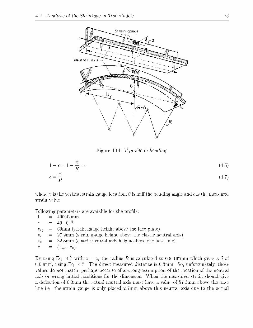
4.2. Analysis of the Shrinkage in Test Models 73
Figure 4.14: T-pro�le in bending.
1 + � = 1 +z
R) (4.6)
� =z
R(4.7)
where z is the vertical strain gauge location, � is half the bending angle and � is the measuredstrain value.
Following parameters are avaiable for the pro�le:l = 400.42mm� = 40 10�6
zsg = 60mm (strain gauge height above the face plate)ze = 27.2mm (strain gauge height above the elastic neutral axis)z0 = 32.8mm (elastic neutral axis height above the base line)z = (zsg - z0)
By using Eq. 4.7 with z = ze the radius R is calculated to 6.8 105mm which gives a � of0.03mm, using Eq. 4.3. The direct measured distance is 0.3mm. So, unfortunately, thosevalues do not match, perhaps because of a wrong assumption of the location of the neutralaxis or wrong initial conditions for the dimension. When the measured strain should givea de ection of 0.3mm the actual neutral axis must have a value of 57.3mm above the baseline i.e. the strain gauge is only placed 2.7mm above this neutral axis due to the actual
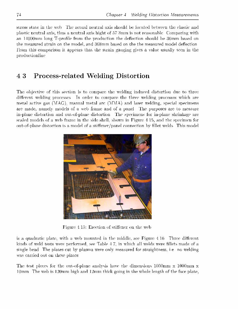
74 Chapter 4. Welding Distortion Measurements
stress state in the web. The actual neutral axis should be located between the elastic andplastic neutral axis, thus a neutral axis hight of 57.3mm is not reasonable. Comparing withan 14000mm long T-pro�le from the production the de ection should be 36mm based onthe measured strain on the model, and 368mm based on the the measured model de ection.From this comparison it appears that the strain gauging gives a value usually seen in theproductionline.
4.3 Process-related Welding Distortion
The objective of this section is to compare the welding induced distortion due to threedi�erent welding processes. In order to compare the three welding processes which aremetal active gas (MAG), manual metal arc (MMA) and laser welding, special specimensare made, namely models of a web frame and of a panel. The purposes are to measurein-plane distortion and out-of-plane distortion. The specimens for in-plane shrinkage arescaled models of a web frame in the side shell, shown in Figure 4.15, and the specimen forout-of-plane distortion is a model of a sti�ener/panel connection by �llet welds. This model
Figure 4.15: Erection of sti�ener on the web.
is a quadratic plate, with a web mounted in the middle, see Figure 4.16. Three di�erentkinds of weld tests were performed, see Table 4.7, in which all welds were �llets made of asingle bead. The plates cut by plasma were only measured for straightness, i.e. no weldingwas carried out on these plates.
The test pieces for the out-of-plane analysis have the dimensions 1000mm x 1000mm x10mm. The web is 120mm high and 12mm thick going in the whole length of the face plate,
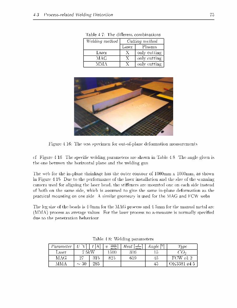
4.3. Process-related Welding Distortion 75
Table 4.7: The di�erent combinations.
Welding method Cutting methodLaser Plasma
Laser X only cuttingMAG X only cuttingMMA X only cutting
Figure 4.16: The test specimen for out-of-plane deformation measurements.
cf. Figure 4.16. The speci�c welding parameters are shown in Table 4.8. The angle given isthe one between the horizontal plane and the welding gun.
The web for the in-plane shrinkage has the outer contour of 1000mm x 1000mm, as shownin Figure 4.15. Due to the performance of the laser installation and the size of the scanningcamera used for aligning the laser head, the sti�eners are mounted one on each side insteadof both on the same side, which is assumed to give the same in-plane deformation as thepractical mounting on one side. A similar geometry is used for the MAG and FCW webs.
The leg size of the beads is 4.0mm for the MAG process and 4.5mm for the manual metal arc(MMA) process as average values. For the laser process no a-measure is normally speci�eddue to the penetration behaviour.
Table 4.8: Welding parameters.
Parameter U [V] I [A] v [mmmin
] Heat [ Jmm
] Angle [0] TypeLaser 7.5kW 1500 316 15 CO2
MAG 27 315 825 619 45 FCW �1.2MMA � 30 285 { { 45 OK3381 �4.5

76 Chapter 4. Welding Distortion Measurements
Table 4.9: Statistical values for the out-of-plane de ection.
Process Mean value � [mm] Standard deviation �Laser 0.54 0.69MAG 15.06 1.62
Electrode 19.08 1.72
Out-of-plane measurements were made with a ruler and a straight pin. The out-of-planeresults in Table 4.9 show that welding with a MMA (electrodes) gives a de ection which isslightly larger than the de ection for the MAG processes, whereas the laser method gives asigni�cant smaller de ection.
It can also be seen that the variation is smaller for the laser welding. Hence, the data forthe laser welding process is located more homogeneously around the mean value than forthe MMA or MAG welds, which indicates that the laser welding is a more uniform weldingprocess. This is due to both the process and the high-precision steering of the laser processand mechanics.
The in-plane shrinkage is measured with the high-performance measuring equipment MON-MOS. A co-ordinate system is aligned with the X-axis through points 1 and 2, as shown inFigure 4.17.
The in uence of the processes on the in-plane shrinkage can be seen in Table 4.10, where themovement of point 5 parallel with the X-axis is tabulated. For the in-plane shrinkage only
Table 4.10: In-plane shrinkage, [mm].
Process Shrinkage [mm] Mean [mm]Laser 3.05 1.22 1.11 1.81 1.43 1.7MAG 4.63 6.48 1.9 5.95 5.96 5.0MMA 5.56 7.05 5.42 | 6.23 6.0
one measurement per point per plate - i.e. �ve measurements for alignment and angle foreach process - is available. The in-plane displacement given is related to the X-axis betweenpoints 1 and 2, illustrated in Figure 4.17.
As shown in Table 4.10, the laser process gives signi�cantly less in-plane shrinkage than thetwo other processes.
The straightness of the corner (at point 1 in Figure 4.17) is measured and the results areshown in Table 4.11. 30 specimens in total have been measured, i.e. �ve specimens perprocess.

4.3. Process-related Welding Distortion 77
Figure 4.17: The web specimen with the sti�ener, the used co-ordinate system, and thelocation of measure points.
Both processes cut with a high accuracy.
The three processes dealt with here operate with signi�cantly di�erent welding parameters.Moreover, the heat input is di�erent and thus, also the thermal zones (HAZ), see Figure4.18.
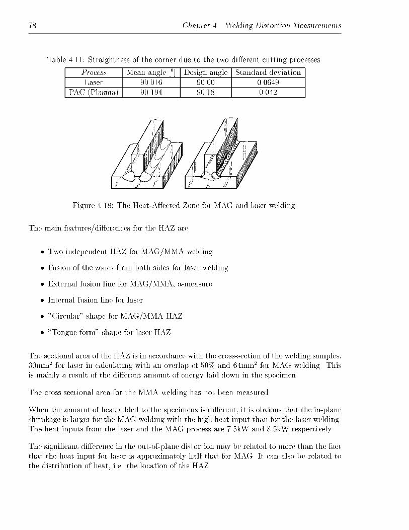
78 Chapter 4. Welding Distortion Measurements
Table 4.11: Straightness of the corner due to the two di�erent cutting processes.
Process Mean angle [0] Design angle Standard deviationLaser 90.016 90.00 0.0649
PAC (Plasma) 90.194 90.18 0.042
Figure 4.18: The Heat-A�ected Zone for MAG and laser welding.
The main features/di�erences for the HAZ are
� Two independent HAZ for MAG/MMA welding
� Fusion of the zones from both sides for laser welding
� External fusion line for MAG/MMA, a-measure
� Internal fusion line for laser
� "Circular" shape for MAG/MMA HAZ
� "Tongue form" shape for laser HAZ
The sectional area of the HAZ is in accordance with the cross-section of the welding samples,30mm2 for laser in calculating with an overlap of 50% and 64mm2 for MAG welding. Thisis mainly a result of the di�erent amount of energy laid down in the specimen.
The cross sectional area for the MMA welding has not been measured.
When the amount of heat added to the specimens is di�erent, it is obvious that the in-planeshrinkage is larger for the MAG welding with the high heat input than for the laser welding.The heat inputs from the laser and the MAG process are 7.5kW and 8.5kW respectively.
The signi�cant di�erence in the out-of-plane distortion may be related to more than the factthat the heat input for laser is approximately half that for MAG. It can also be related tothe distribution of heat, i.e. the location of the HAZ.

4.3. Process-related Welding Distortion 79
The hand welding with electrodes gives the highest de ection (approximately 30% morethan for the MAG process), which is partly because of the higher a-measure (4.5mm against4.0mm, which gives an increase in the sectional area of 25%) and partly due to the di�erentHAZ.
The angular distortion is signi�cant lower for the laser process than for the MAG, becauseof the signi�cant di�erence in a-measure and the welding process itself.
The study has proved that the laser process gives much less in-plane shrinkage, and especiallyout-of-plane distortion, compared with the MAG and MMA welding.

80 Chapter 4. Welding Distortion Measurements
This page is intentionally left blank.
Chapter 5
Thermomechanical Analysis Using
FEM
5.1 Introduction
When a commercial FEM program is to be chosen, four main issues should be considered:functionality, computational e�ciency, ease of use and ease of learning. Because most ofthe time dealing with �nite element modelling concerns data preparation and test runs, thelatter two items are nearly as important as functionality.
By a literature study and from experience with di�erent FEM programs as ABAQUSTM
and NISATM see Appendix A, the program SYSTUS+ c was selected. The experienceswith NISA is presented in [4].
SYSTUS+ is divided in two applications:
� A geometry/meshing application used to model a mechanical structure. This structurecan also be retrieved from CAD software by means of an interface such as IGES, STEPand VAD.
� An analysis application subdivided in several analysis modules is used, �rst to build the�nite element model with its physical numerical properties, then to solve the problem.
Fore more information about SYSTUS+, see [16].
The SYSWELD+ software, directly derived from the SYSTUS+ system, is able to determineresidual stresses and strains resulting from welding or heat treatments (quenching, induction,surface treatment) as well as di�usion precipitation and hydrogen di�usion.
82 Chapter 5. Thermomechanical Analysis Using FEM
The software can compute the link between the structure, the residual stress and the hydro-gen di�usion by integrating the e�ects of metallurgical transformation.
The main di�erences from other FEM programs are, [55]:
1. Thermal and metallurgical calculations, which can couple temperatures and phaseproperties. Thus, in the equation expressing conduction of heat in the transient state,the latent heat of solidi�cation and metallurgical transformations can be taken intoaccount. At the end of the �rst stage, the information available for each elementof material includes not only its thermal history but also its metallurgical history(proportions of phases, austenitic grain size).
2. The coupling between electro-kinetic, thermal and metallurgical equations, which makesit possible on one hand, to account for the variation of electrical properties as a func-tion of temperature and, on the other hand, to account for heat sources resulting fromthe Joule e�ect and metallurgical phase transformations.
3. Mechanical plasticity calculations which depend not only on temperature but also onthe metallurgical history of the elements.
4. Hydrogen di�usion calculation, which includes (depending on the degree of accuracyrequired) the e�ects of temperature, metallurgical transformation, stresses, plastic de-formations, inclusions and non-uniform solubility.
5. Modelling of di�usion and/or precipitation of chemical elements prior to heat treat-ment.
Graphically, the structure of SYSTUS+ is as depicted in Figure 5.1.
The main purpose of the study is to investigate the deformation due to a weld, and not somuch the weld mechanics itself. Therefore, phase transformations are not taken into account.Mechanical properties such as fracture toughness, ductile-brittle transition temperature andhydrogen di�usion are not included either, because it is assumed that these e�ects accountfor an insigni�cant contribution to the total solution.
5.2 Thermal FE Analysis
Thermal problems which can be solved in advance by using the FEM may roughly be dividedinto three categories:The �rst category concerns thermal problems at a steady state involving constant thermo-physical properties. The second category concerns problems in a transient state with constantthermophysical properties and boundary conditions which may depend on time but not ontemperature. The aim is here to compute the change in temperature in the course of time

5.2. Thermal FE Analysis 83
Figure 5.1: Structure of SYSWELD, [56].
starting from an initial state. Finally, the third category covers all the stationary or non-stationary problems including non-linearities or the heat transfer coe�cient varying withtime and temperature.
The boundary conditions are applied to the model by specifying the value of the heat transfercoe�cient h and the surrounding temperatures for the elements and at the nodes, respec-tively, of the skin elements obtained by creating a mesh on the surface of the structuraldomain. For a 2D problem, the skin elements are 1D elements and for a 3D problem, theskin elements are 2D elements.When applied to the heat equation, the �nite element method involves the solution of asystem of di�erential equations:
C _T+KT = Q (5.1)
where T represents the nodal temperature vector, _T is the time derivative of temperature,C is the speci�c heat matrix ( J
K), K the conductivity matrix (W
K), and Q the vector of nodal
powers equivalent to an internal heat source and boundary conditions. Eq. 5.1 is derived byuse of shape (or interpolation) functions, see e.g. [12]. Under static conditions, this systemis reduced to
KT = Q (5.2)

84 Chapter 5. Thermomechanical Analysis Using FEM
Eq. 5.1 can be written
R = Q�C _T�KT = 0 (5.3)
where R represents a table containing all the residual nodal forces (temperatures). Fornon-linear problems, Eq. 5.3 must be solved at each time instant by an iterative method.
If R is taken to be the residue resulting from the ith iteration, i.e. obtained with a tempe-rature �eld Ti, then an improved solution could be obtained by writing
Ri+1 = Ri +
@R
@T
!i
�Ti = 0 (5.4)
where�@R@T
�irepresents the tangent matrix resulting from the ith iteration. Thus
�Ti = � @R
@T
!�1i
Ri (5.5)
is obtained either iteratively or directly by Choleski factorisation and yields the new approx-imation
Ti+1 = Ti + �Ti (5.6)
This procedure is repeated until the norm of the residue
kRi+1k � �m (5.7)
where �m is a small parameter speci�ed by the user.
The matrix�@R@T
��1i
is only used to provide a tangent sti�ness matrix for an improved tempe-
rature vector. Hence, it is not necessary to recompute it at each iteration. As the iterativesolution method BFGS (quasi-newton), see [32] has been chosen, the left-hand side matrixcorresponds to the secant matrix between two successive iterations.

5.3. Mechanical FE Analysis 85
5.3 Mechanical FE Analysis
5.3.1 Equilibrium Equations
A static linear analysis is used to determine the response of a structure subjected to any setof loads, where the behaviour of the structure is not in uenced by
� Time factor and dynamic e�ects (inertia and damping in particular)
� Non-linearities of any origin (geometric, material, contact, etc.)
The equation governing this type of behaviour is
KsU = F (5.8)
where Ks is the sti�ness matrix, U is the displacement vector for the structure, and F theexternal load vector. The force vector F may include thermal loads or initial strains.
The basic equation governing the dynamic behaviour of a structure, is
M�U+C _U +KU = F(t) (5.9)
When the behaviour of the structure is linear, the matrices K, M and C are independent ofthe displacement.
Two methods of solving this equation are available with SYSTUS+, cf. [56]:
� A method involving utilisation of a representative eigenmode base, referred to as themodal superposition method
� A direct solution method, referred to as the step-by-step time integration method
The analysis of the mechanical system is similar to the analysis of the thermal problem. Forthe non-linear dynamic problem, the �nite element analysis involves repeated solutions ofthe following type:
R = F�KU�C _U�M�U = 0 (5.10)
where R = the residual nodal force vector, K is the sti�ness matrix, C is the damping matrixand M is the mass matrix.

86 Chapter 5. Thermomechanical Analysis Using FEM
5.3.2 Constitutive Equations
A number of plasticity criteria and models are available in SYSTUS:
� Von Mises, Drucker, Stassi, Tsai-Hill are implemented. In addition user-de�ned criteriamay be applied.
� Perfect plasticity models and plasticity models with isotropic, kinematic or combinedstrain hardening in the case of the von Mises criterion. Plasticity models interactingwith ductile damage (germination, growth, and coalescence of cavities).
Experience shows, e.g. [59], that there is a convex domain in the stress space, referred to asthe elastic domain, so that any load path inside this domain generates elastic strains only.This domain is de�ned from a scalar value function Y, referred to as the yield function orthe plasticity criterion:
Y (�ij) � 0 (5.11)
If an elastic stress state reaches the boundary of this domain, plastic strain occurs so thatthe stress state satis�es,
Y (�ij) = 0 (5.12)
This equation de�nes the yield surface in the stress space. The total strain is broken downinto
� Thermal strain
� Elastic strain
� Plastic strain
In incremental form the above strains read
��ij = ��eij +��tij +��pij (5.13)
The existence of a plastic potential (Hill's principle of maximum plastic work, [5]) leads toformulation of a hypothesis of normality, so that the following relation can be written:
��pij = ��@Y
@�ij(5.14)
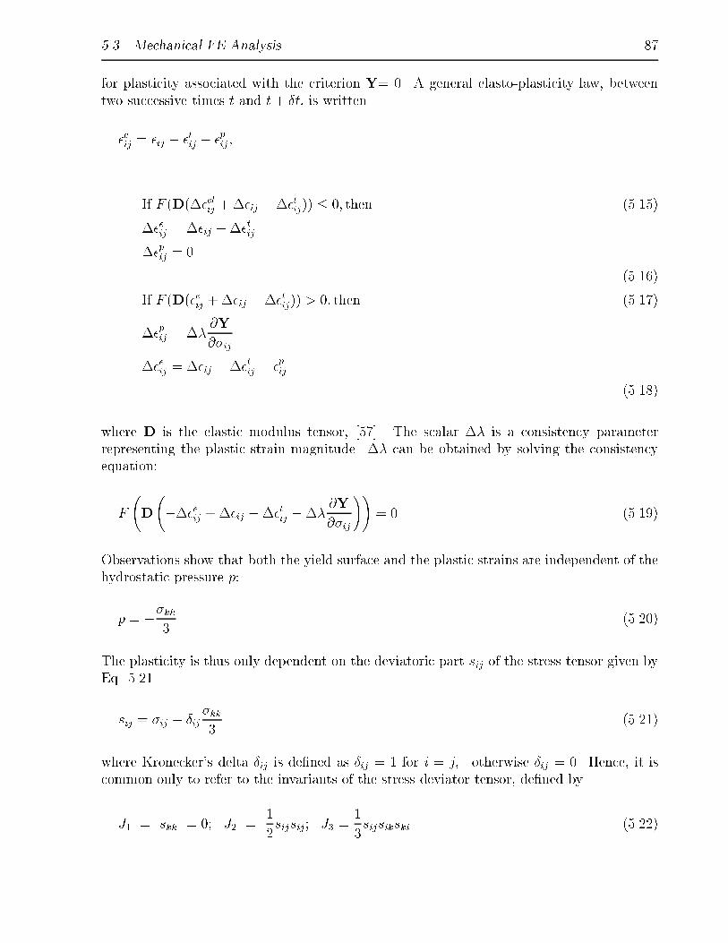
5.3. Mechanical FE Analysis 87
for plasticity associated with the criterion Y= 0. A general elasto-plasticity law, betweentwo successive times t and t + �t, is written
�eij = �ij � �tij � �pij;
If F (D(��elij +��ij ���tij)) � 0; then (5.15)
��eij = ��ij ���tij
��pij = 0
(5.16)
If F (D(�eij +��ij ���tij)) > 0; then (5.17)
��pij = ��@Y
@�ij
��eij = ��ij ���tij � �pij
(5.18)
where D is the elastic modulus tensor, [57]. The scalar �� is a consistency parameterrepresenting the plastic strain magnitude. �� can be obtained by solving the consistencyequation:
F
D
���eij +��ij ���tij ���
@Y
@�ij
!!= 0 (5.19)
Observations show that both the yield surface and the plastic strains are independent of thehydrostatic pressure p:
p = ��kk3
(5.20)
The plasticity is thus only dependent on the deviatoric part sij of the stress tensor given byEq. 5.21.
sij = �ij � �ij�kk3
(5.21)
where Kronecker's delta �ij is de�ned as �ij = 1 for i = j; otherwise �ij = 0. Hence, it iscommon only to refer to the invariants of the stress deviator tensor, de�ned by
J1 = skk = 0; J2 =1
2sijsij; J3 =
1
3sijsikski (5.22)

88 Chapter 5. Thermomechanical Analysis Using FEM
The von Mises yield surface is only dependent on J2.
The von Mises stress yield surface is represented, in the principal stress space, by a circle
with the radiusq
23�y. The von Mises criterion is particularly suitable for analysis of metal
plasticity. The von Mises yield surface (or domain) is de�ned by
�e = �y; for �2e =3
2sijsij (5.23)
The von Mises stress or equivalent stress becomes
�e =q3J2 (5.24)
An important observation in metallic plasticity is the plastic incompressibility, implying thatplastic strains do not generate any change in volume:
�pkk = 0 (5.25)
In practice, the elasticity domain changes in the presence of a plastic strain. This phe-nomenon is referred to as strain-hardening. The plasticity criterion then depends on othervariables, notably the plastic strains. Conventionally, distinction is made between two typesof strain hardening.
Isotropic strain-hardening, which corresponds to "expansion" of the elasticity domain, seeFigure 5.2. By application of the von Mises criterion this expression is governed by a scalarinternal variable �peq, corresponding to the cumulative equivalent plastic strain
�peq =Z t
0
_�peqdt (5.26)
_�peq =
s2
3_�pij_�pij (5.27)
The isotropic strain hardening model is de�ned by
Y (�ij; �peq) = �e � �0(T; �
peq) (5.28)
with �0(T; �peq = 0) = �y(T ) as the initial yield stress of the material at the actual tempe-
rature.

5.3. Mechanical FE Analysis 89
Figure 5.2: Isotropic strain-hardening. Figure 5.3: Kinematic strain-hardening.
Figure 5.4: Strain-hardening slope depending on both plastic strain and temperature.
SYSTUS+ enables the user to enter the strain-hardening law point by point or to apply aRamberg-Osgood law reading
� =�
E+ �
�yE
�
�y
!n(5.29)
where � is a constant experimentally determined to be approximately 0.1, [59]. n is thehardening exponent, approximately 5 for steel alloys, and E is Young's modulus.
The other strain hardening model is kinematic strain-hardening, which corresponds to atranslation of the elasticity domain in the stress space, Figure 5.3. Kinematic strain-hardening models can be used to represent the Bauschinger e�ect (behavioural anisotropyunder tensile - compression loads) and are consequently recommended for cyclic applications.
The degree of strain-hardening depends on various parameters such as the temperature-dependent yield stresses and the strain-hardening slope depending on the plastic strain(zero for perfect plasticity). The last item is illustrated in Figure 5.4. The elasto-plastic
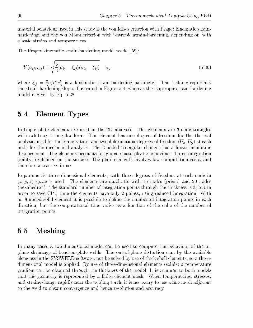
90 Chapter 5. Thermomechanical Analysis Using FEM
material behaviour used in this study is the von Mises criterion with Prager kinematic strain-hardening, and the von Mises criterion with isotropic strain-hardening, depending on bothplastic strains and temperatures.
The Prager kinematic strain-hardening model reads, [59]:
Y (�ij; �ij) =
s3
2(�ij � �ij)(�ij � �ij)� �y (5.30)
where �ij = 23c(T )�pij is a kinematic strain-hardening parameter. The scalar c represents
the strain-hardening slope, illustrated in Figure 5.4, whereas the isoptropic strain-hardeningmodel is given by Eq. 5.28.
5.4 Element Types
Isotropic plate elements are used in the 2D analyses. The elements are 3-node triangleswith arbitrary triangular form. The element has one degree of freedom for the thermalanalysis, used for the temperature, and two deformations degrees-of-freedom (Ux, Uy) at eachnode for the mechanical analysis. The 3-noded triangular element has a linear membranedisplacement. The elements accounts for global elasto-plastic behaviour. Three integrationpoints are de�ned on the surface. The plate elements involves low computation costs, andtherefore attractive in use.
Isoparametric three-dimensional elements, with three degrees of freedom at each node in(x; y; z) space is used. The elements are quadratic with 15 nodes (prism) and 20 nodes(hexahedron). The standard number of integration points through the thickness is 3, but inorder to save CPU time the elements have only 2 points, using reduced integration. Withan 8-noded solid element it is possible to de�ne the number of integration points in eachdirection, but the computational time varies as a function of the cube of the number ofintegration points.
5.5 Meshing
In many cases a two-dimensional model can be used to compute the behaviour of the in-plane shrinkage of bead-on-plate welds. The out-of-plane distortion can, by the availableelements in the SYSWELD software, not be solved by use of thick shell elements, so a three-dimensional model is applied. By use of three-dimensional elements (solids) a temperaturegradient can be obtained through the thickness of the model. It is common to both modelsthat the geometry is represented by a �nite element mesh. When temperatures, stresses,and strains change rapidly near the welding torch, it is necessary to use a �ne mesh adjacentto the weld to obtain convergence and hence resolution and accuracy.
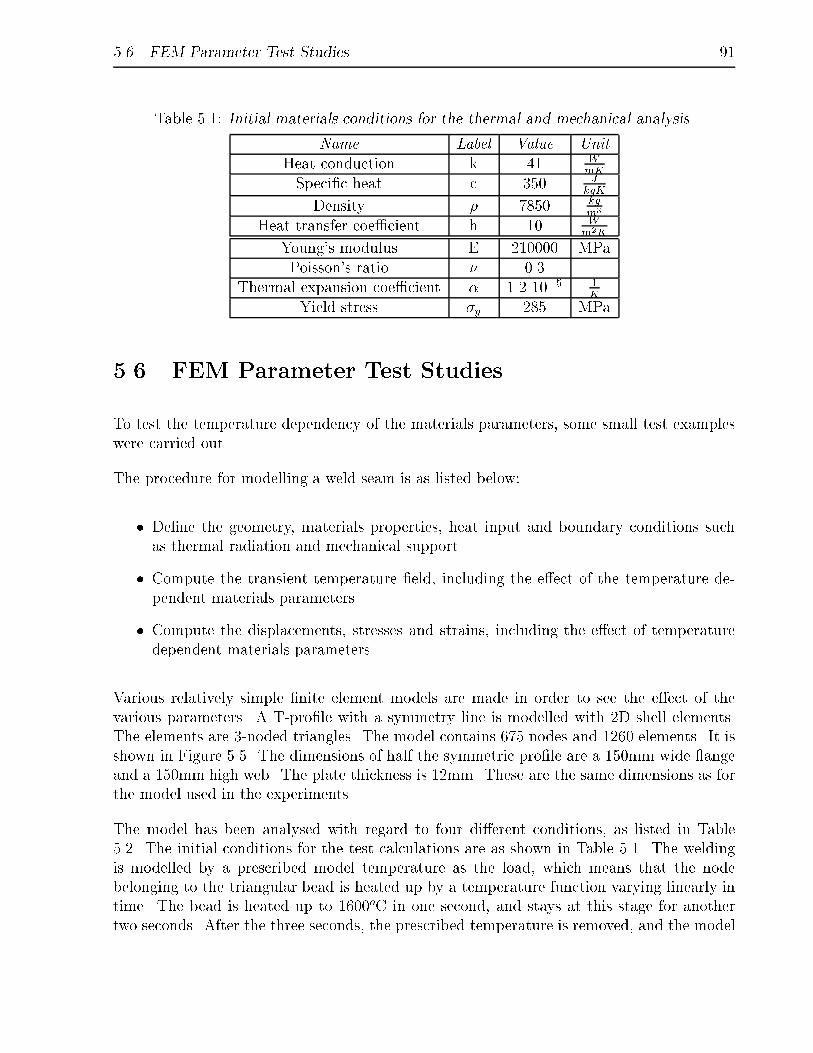
5.6. FEM Parameter Test Studies 91
Table 5.1: Initial materials conditions for the thermal and mechanical analysis.
Name Label Value UnitHeat conduction k 41 W
mK
Speci�c heat c 350 JkgK
Density � 7850 kgm3
Heat transfer coe�cient h 10 Wm2K
Young's modulus E 210000 MPaPoisson's ratio � 0.3 |
Thermal expansion coe�cient � 1.2 10�5 1K
Yield stress �y 285 MPa
5.6 FEM Parameter Test Studies
To test the temperature dependency of the materials parameters, some small test exampleswere carried out.
The procedure for modelling a weld seam is as listed below:
� De�ne the geometry, materials properties, heat input and boundary conditions suchas thermal radiation and mechanical support.
� Compute the transient temperature �eld, including the e�ect of the temperature de-pendent materials parameters.
� Compute the displacements, stresses and strains, including the e�ect of temperaturedependent materials parameters.
Various relatively simple �nite element models are made in order to see the e�ect of thevarious parameters. A T-pro�le with a symmetry line is modelled with 2D shell elements.The elements are 3-noded triangles. The model contains 675 nodes and 1260 elements. It isshown in Figure 5.5. The dimensions of half the symmetric pro�le are a 150mm wide angeand a 150mm high web. The plate thickness is 12mm. These are the same dimensions as forthe model used in the experiments.
The model has been analysed with regard to four di�erent conditions, as listed in Table5.2. The initial conditions for the test calculations are as shown in Table 5.1. The weldingis modelled by a prescribed model temperature as the load, which means that the nodebelonging to the triangular bead is heated up by a temperature function varying linearly intime. The bead is heated up to 1600oC in one second, and stays at this stage for anothertwo seconds. After the three seconds, the prescribed temperature is removed, and the model
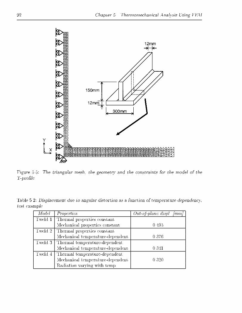
92 Chapter 5. Thermomechanical Analysis Using FEM
Figure 5.5: The triangular mesh, the geometry and the constraints for the model of theT-pro�le.
Table 5.2: Displacement due to angular distortion as a function of temperature dependency,test example.
Model Properties Out-of-plane displ. [mm]Tweld 1 Thermal properties constant
Mechanical properties constant 0.495Tweld 2 Thermal properties constant
Mechanical temperature-dependent 0.376Tweld 3 Thermal temperature-dependent
Mechanical temperature-dependent 0.341Tweld 4 Thermal temperature-dependent
Mechanical temperature-dependent 0.320Radiation varying with temp.

5.6. FEM Parameter Test Studies 93
cools down by the boundary conditions which are given a heat transfer coe�cient, in orderto simulate the boundaries of the model as the heat exchanges surfaces. The displacementsshown in Table 5.2 are the vertical displacement of the ange plate 150mm from the centreline. The comparative study shown in Table 5.2 clearly indicates that the in uence oftemperature on especially the mechanical parameters is signi�cant for the displacement.
The di�erence in the de ection is more than 30% if all temperature dependencies are takeninto account compared to the model with temperature-independent parameters. The mate-rials parameter dependency on temperature are illustrated in Figure 5.9.
5.6.1 Temperature Dependency in the Thermal Part
Based on experiments and knowledge obtained from the application development group atSYSTUS, then temperature load is applied as stated previously. In order to validate thereliability of this speci�c load case, some other "heating pro�les" is applied the model ofthe 2D T-pro�le, for comparing the residual de ection of the ange plate 150mm from thecentre line. The results are shown in Figure 5.6. It should be noted that the FEM modelaccounts for heat losses by radiation and convection already from the start of heating, e.g.from the time t = 0 secs, which in uences the global heating of the model. As Figure 5.6shows the variation in de ection is relative small, from 0.7mm to 1.9mm, when only heatingup to 16000C, which is a little above the melting temperature for the steel. A higher heatinput, related to a higher temperature of the bead elements give a drastic increase in the out-of-plane de ection. An overall temperature of the bead elements higher than approximately16000C is assumed much to unrealistic. Hence, the applied temperature pro�le for thethermal load case is assumed to be usable. Of course it is only an assumption, because thecross-section of the bead is a steady picture of a transient heat source.
The heat transfer coe�cient is the thermal equivalent of an elastic constraint. This is acondition which is normally applied to a surface of the elements. Because of its nature, thiscondition can be de�ned either as a constraint or as a load (temperature). Table 5.3 showsthe results for di�erent values of the heat transfer coe�cient h. An average value of the heattransfer coe�cient for this speci�c case could be approximately 100 W
m2K.
The in uence of the yield stress on the angular displacement of the FEM model is shownin Table 5.4 and Figure 5.7. The results show that the yield limit has a more signi�cantin uence on the residual de ection for the temperature-independent yield stress than forthe temperature-dependent yield stress. The temperature dependency of the yield stressintroduces a de ection variation of approximately 4% in the interval from 200 MPa to 500MPa. The temperature-independent yield stress gives a change of approximately 20% in thesame interval. This was also expected, because the yield stress decreases very much in therelative low temperature interval.
In order to test how important the a-measure size is to the distortion, as illustrated by theangular displacement in mm, three di�erent a-measure sizes are considered. The leg length
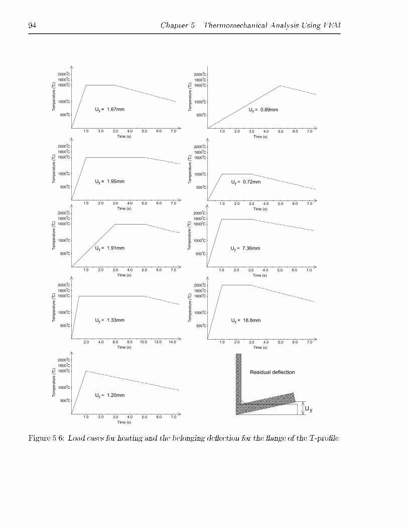
94 Chapter 5. Thermomechanical Analysis Using FEM
Figure 5.6: Load cases for heating and the belonging de ection for the ange of the T-pro�le.
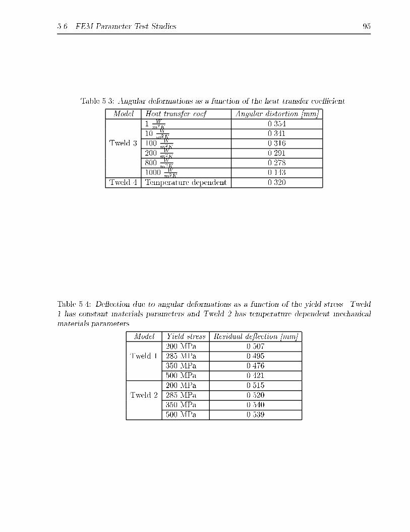
5.6. FEM Parameter Test Studies 95
Table 5.3: Angular deformations as a function of the heat transfer coe�cient.
Model Heat transfer coef. Angular distortion [mm]1 W
m2K0.354
10 Wm2K
0.341Tweld 3 100 W
m2K0.316
200 Wm2K
0.291800 W
m2K0.278
1000 Wm2K
0.143Tweld 4 Temperature dependent 0.320
Table 5.4: De ection due to angular deformations as a function of the yield stress. Tweld1 has constant materials parameters and Tweld 2 has temperature dependent mechanicalmaterials parameters.
Model Yield stress Residual de ection [mm]200 MPa 0.507
Tweld 1 285 MPa 0.495350 MPa 0.476500 MPa 0.421200 MPa 0.515
Tweld 2 285 MPa 0.520350 MPa 0.540500 MPa 0.539
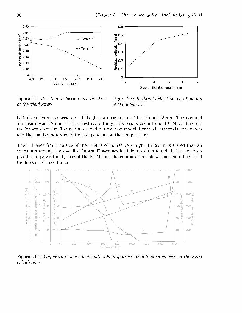
96 Chapter 5. Thermomechanical Analysis Using FEM
Figure 5.7: Residual de ection as a functionof the yield stress.
Figure 5.8: Residual de ection as a functionof the �llet size.
is 3, 6 and 9mm, respectively. This gives a-measures of 2.1, 4.2 and 6.3mm. The nominala-measure was 4.2mm. In these test cases the yield stress is taken to be 350 MPa. The testresults are shown in Figure 5.8, carried out for test model 4 with all materials parametersand thermal boundary conditions dependent on the temperature.
The in uence from the size of the �llet is of course very high. In [22] it is stated that anextremum around the so-called "normal" a-values for �llets is often found. It has not beenpossible to prove this by use of the FEM, but the computations show that the in uence ofthe �llet size is not linear.
Figure 5.9: Temperature-dependent materials properties for mild steel as used in the FEMcalculations.
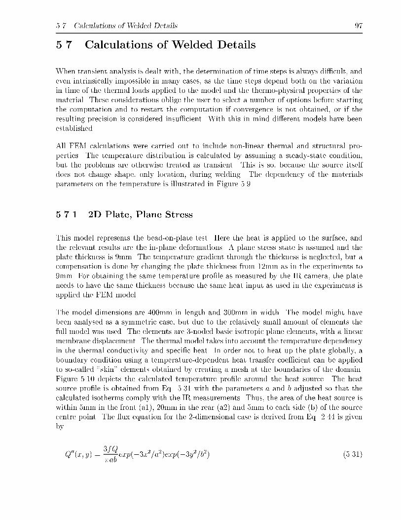
5.7. Calculations of Welded Details 97
5.7 Calculations of Welded Details
When transient analysis is dealt with, the determination of time steps is always di�cult, andeven intrinsically impossible in many cases, as the time steps depend both on the variationin time of the thermal loads applied to the model and the thermo-physical properties of thematerial. These considerations oblige the user to select a number of options before startingthe computation and to restart the computation if convergence is not obtained, or if theresulting precision is considered insu�cient. With this in mind di�erent models have beenestablished.
All FEM calculations were carried out to include non-linear thermal and structural pro-perties. The temperature distribution is calculated by assuming a steady-state condition,but the problems are otherwise treated as transient. This is so, because the source itselfdoes not change shape, only location, during welding. The dependency of the materialsparameters on the temperature is illustrated in Figure 5.9.
5.7.1 2D Plate, Plane Stress
This model represents the bead-on-plate test. Here the heat is applied to the surface, andthe relevant results are the in-plane deformations. A plane stress state is assumed and theplate thickness is 9mm. The temperature gradient through the thickness is neglected, but acompensation is done by changing the plate thickness from 12mm as in the experiments to9mm. For obtaining the same temperature pro�le as measured by the IR camera, the plateneeds to have the same thickness because the same heat input as used in the experiments isapplied the FEM model.
The model dimensions are 400mm in length and 300mm in width. The model might havebeen analysed as a symmetric case, but due to the relatively small amount of elements thefull model was used. The elements are 3-noded basic isotropic plane elements, with a linearmembrane displacement. The thermal model takes into account the temperature dependencyin the thermal conductivity and speci�c heat. In order not to heat up the plate globally, aboundary condition using a temperature-dependent heat transfer coe�cient can be appliedto so-called "skin" elements obtained by creating a mesh at the boundaries of the domain.Figure 5.10 depicts the calculated temperature pro�le around the heat source. The heatsource pro�le is obtained from Eq. 5.31 with the parameters a and b adjusted so that thecalculated isotherms comply with the IR measurements. Thus, the area of the heat source iswithin 5mm in the front (a1), 20mm in the rear (a2) and 5mm to each side (b) of the sourcecentre point. The ux equation for the 2-dimensional case is derived from Eq. 2.44 is givenby
Q00(x; y) =3fQ
�abexp(�3x2=a2)exp(�3y2=b2) (5.31)

98 Chapter 5. Thermomechanical Analysis Using FEM
x
y
z
0
147.386
1508.97
298.672449.959601.246752.533903.8191055.111206.391357.68
Max = 1660.25Min = -3.90101 Time 30.000078TempCONTOURS
SY
STU
S+ V
2.0 - HP
-UX
-B.10.20 - Tue A
pr 13 19:27:38 1999
Figure 5.10: Elements and temperature pro�le around a heat source moving at 7 mm/s.
where f is the fraction of heat deposited in the front (ff) and the rear (fr), where ff =0.8 and fr = 1.2. Q00(x; y) has the unit ( W
m2 ). Eq. 5.31 is the 2D version of the Gaussian"bell" (Eq. 2.50), which calculates a temperature pro�le with the same width of the HAZ,as obtained in the experiments.
In SYSWELD+, the heat ux value is given by the label QR is de�ned a priori with respectto the dimension of the element. Thus on a 2D element, QR indicates a surface density ofthermal ux and on a 3D element, a volume density.
In Figure 5.11 a comparison is shown for the temperature distribution along the surface ofthe work piece across the weld. As seen in Figure 5.11 the peak temperature obtained by aFEM calculation is relative low, approximately 1650oC. For comparison temperature curvesobtained by Christensen [11], Goldak [20] and Krutz [33]. Their experiments are done onheavy slabs using submerged arc welding, which is as very high powered process. The sourcearea is modelled in such a way that for a given -high- heat input, the peak temperature iskept below 2000oC. When using a volumetric heat source the ration between heat input,volume and temperature should always be approximately the same.
The calculation took 1360 secs for the thermal part and 568 secs for the mechanical part.The size of the model is 2442 elements with 1222 nodes. The smallest size of the elements

5.7. Calculations of Welded Details 99
Figure 5.11: Temperature distribution along the top of a thick plate, perpendicular to theweld, after quasi-steady state has been reached. The welding speed approximately 5mm/s.
is 4mm. It should be noted that the �nal temperature here is 130oC, due to the low heatradiation assumed, in order not to in uence the results in a negative way because of amismatch between heat source and boundary elements. The temperature in the plate attime 2 hours after welding is displayed in Figure 5.12. This actual �nal temperature level isnot so signi�cant, because it is still "cold" compared to the maximum temperature.
The longitudinal shrinkage after cooling is shown in Figure 5.13. The shrinkage at the weldline is 0.032mm, which is much to low. The numerical value of this is approximately afactor of 10 too low compared to the measured value, but the trend is clear, namely thatthe material around the weld line �rst elongates and afterwards during the cooling shrinks.As seen in the experiments the tension forces do not pull the weld line material back intoa position shorter than the initial material, so the overall length shows extension. Thetransverse shrinkage is largest at the middle of the plate of 0.035mm, which also is a muchtoo low a value. The shrinkage values after cooling are shown in Table 5.5.The results should be comparable because the geometry of the FEMmodel and the specimenused in the thermal and shrinkage experiments is the same. The shrinkage calculated bythe FEA and the experimentally obtained shrinkage values are not similar but the relativedi�erence between them is almost the same. The reason to this deviation is not known.

100 Chapter 5. Thermomechanical Analysis Using FEM
x
y
z
0
130.37
130.539
130.388130.407130.426130.445130.464130.483130.502130.52
Max = 130.558Min = 130.351 Time 3599.999512TempCONTOURS
SY
STU
S+ V
2.0 - HP
-UX
-B.10.20 - Tue A
pr 13 19:29:17 1999
Figure 5.12: Temperature in the plate af-ter cooling.
x
y
z
0
-1.3494e-05
0.000106566
-1.5405e-071.31859e-052.65259e-053.98658e-055.32058e-056.65457e-057.98857e-059.32256e-05
Max = 0.000119906Min = -2.6834e-05 Deformed shape X 1000.000000Time 7200.000000Ux
CONTOURS
SY
SW
ELD
+ V 2.0 - H
P-U
X-B
.10.20 - Tue Apr 13 14:48:40 1999
Figure 5.13: Deformation of the plate, leg-end text for longitudinal shrinkage.
Table 5.5: The maximum shrinkage for the 2D plate.
Longitudinal shrinkage adjacent to the weld line 0.032mmTransverse shrinkage at the middle of the plate 0.035mm
Experimentally determined longitudinal shrinkage 0.13mmExperimentally determined transverse shrinkage 0.12mm
5.7.2 Elastoplastic Models
Numerical experiments have shown that using a plasticity model with isotropic strain-hardening where the yield surface is expanding gives results which have a better accordancewith the measured angular distortion than a plasticity model with Prager kinematic strain-hardening. Both models are based on the von Mises criterion. The isotropic model gives ingeneral an easier convergence. This model is therefore used in the following calculations.
5.7.3 T-pro�le, Plane Strain (2D)
The model analysed here is the one used previously in Figure 5.5. The purpose of this two-dimensional model is to calculate the out-of-plane distortion for a �llet weld. The modelis built up of 2D plane strain elements. The plane strain assumption is reasonable in thisspeci�c case because of the 2D cross sectional model. For symmetry reasons only half ofthe structure is modelled. The geometry of the pro�le is as follows: Web height = 150mm, ange = 300mm, length = 400mm. The �llet bead has a size of 5mm. In accordance with[60] the e�ect of gap can be neglected in the FEM modelling. The gap has only some e�ecton the local transverse residual stresses near the gap and in the web, but it has very smalle�ect on residual stresses in the ange. The following models are therefore modelled without
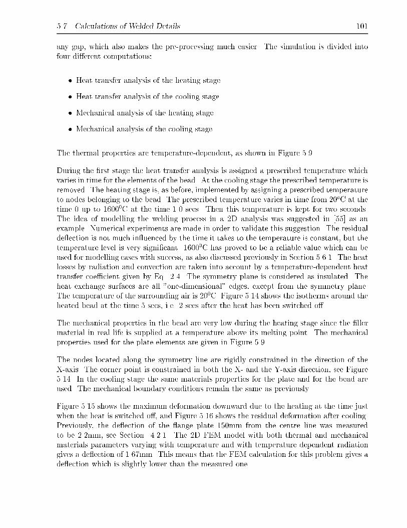
5.7. Calculations of Welded Details 101
any gap, which also makes the pre-processing much easier. The simulation is divided intofour di�erent computations:
� Heat transfer analysis of the heating stage
� Heat transfer analysis of the cooling stage
� Mechanical analysis of the heating stage
� Mechanical analysis of the cooling stage
The thermal properties are temperature-dependent, as shown in Figure 5.9.
During the �rst stage the heat transfer analysis is assigned a prescribed temperature whichvaries in time for the elements of the bead. At the cooling stage the prescribed temperature isremoved. The heating stage is, as before, implemented by assigning a prescribed temperatureto nodes belonging to the bead. The prescribed temperature varies in time from 20oC at thetime 0 up to 16000C at the time 1.0 secs. Then this temperature is kept for two seconds.The idea of modelling the welding process in a 2D analysis was suggested in [55] as anexample. Numerical experiments are made in order to validate this suggestion. The residualde ection is not much in uenced by the time it takes to the temperature is constant, but thetemperature level is very signi�cant. 16000C has proved to be a reliable value which can beused for modelling cases with success, as also discussed previously in Section 5.6.1. The heatlosses by radiation and convection are taken into account by a temperature-dependent heattransfer coe�cient given by Eq. 2.4. The symmetry plane is considered as insulated. Theheat exchange surfaces are all "one-dimensional" edges, except from the symmetry plane.The temperature of the surrounding air is 200C. Figure 5.14 shows the isotherms around theheated bead at the time 5 secs, i.e. 2 secs after the heat has been switched o�.
The mechanical properties in the bead are very low during the heating stage since the �llermaterial in real life is supplied at a temperature above its melting point. The mechanicalproperties used for the plate elements are given in Figure 5.9.
The nodes located along the symmetry line are rigidly constrained in the direction of theX-axis. The corner point is constrained in both the X- and the Y-axis direction, see Figure5.14. In the cooling stage the same materials properties for the plate and for the bead areused. The mechanical boundary conditions remain the same as previously.
Figure 5.15 shows the maximum deformation downward due to the heating at the time justwhen the heat is switched o�, and Figure 5.16 shows the residual deformation after cooling.Previously, the de ection of the ange plate 150mm from the centre line was measuredto be 2.2mm, see Section 4.2.1. The 2D FEM model with both thermal and mechanicalmaterials parameters varying with temperature and with temperature dependent radiationgives a de ection of 1.67mm. This means that the FEM calculation for this problem gives ade ection which is slightly lower than the measured one.
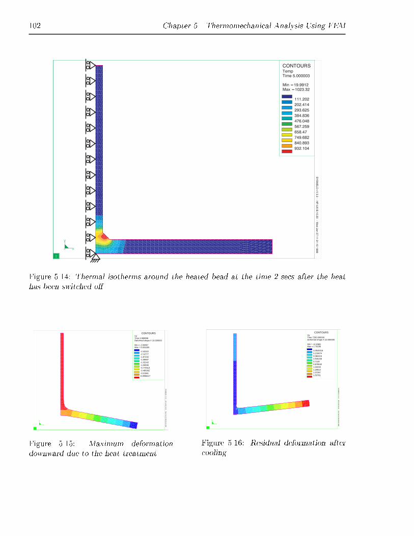
102 Chapter 5. Thermomechanical Analysis Using FEM
Figure 5.14: Thermal isotherms around the heated bead at the time 2 secs after the heathas been switched o�.
x
y
z
0
-2.42322
0.0558417
-2.14777-1.87232-1.59687-1.32142-1.04596-0.770513-0.495062-0.21961
Max = 0.331293Min = -2.69867 Deformed shape X 10.000000Time 2.999998Uy
CONTOURS
SY
SW
ELD
+ V 2.0 - H
P-U
X-B
.10.20 - Mon Feb 22 08:28:16 1999
Figure 5.15: Maximum deformationdownward due to the heat treatment.
x
y
z
0
0.0549318
1.53761
0.2196740.3844160.5491580.71390.8786421.043381.208131.37287
Max = 1.70235Min = -0.10981 Deformed shape X 10.000000Time 7200.000000Uy
CONTOURS
SY
SW
ELD
+ V 2.0 - H
P-U
X-B
.10.20 - Mon Feb 22 08:29:28 1999
Figure 5.16: Residual deformation aftercooling.

5.7. Calculations of Welded Details 103
Figure 5.17: The residual longitudinal stresses in the T-pro�le after cooling compared withmeasured values.
During the cooling stage the heat-a�ected material shrinks due to the plastic e�ect. Themaximum downward bending was just seen when the heat was switched o� for the FE calcu-lation and the maximum shrinkage level was reached after approximately 20 secs. Afterwardsthe residual de ection was constant. For the experiments the maximum shrinkage was seena few seconds after the heat has been switched o�. Afterwards the ange plate fell down alittle. This phenomenon is illustrated in Figure 5.18. The "spring-back" cannot be statedas a constant value because the experiments (Figure 5.18) only show "spring-back" for the�rst �llet and not for the second �llet. This may be due to the constraint of the structureafter laying down the �rst �llet. Due to the severe constraint for the T-pro�le model usedin the experiments, the downward de ection cannot be expected to be as large as for the 2DFEM model, which is a cross-section of the pro�le and, hence, cannot have any constraintfrom the adjacent section for downward bending at the heating stage. The phenomena isillustrated in Figure 5.19.
It is seen from the Figures 5.18 and 5.19 that the isotropic-hardening model gives predictionsof the residual de ection in better agreement with the measurements than the kinematic-hardening model. The calculated and experimental longitudinal residual stresses are plottedin Figure 5.17 and a reasonable agreement is found.

104 Chapter 5. Thermomechanical Analysis Using FEM
Figure 5.18: De ection curves obtained by the present experiments and FEM anal-yses.
Figure 5.19: De ection curves during the �rst two minutes.
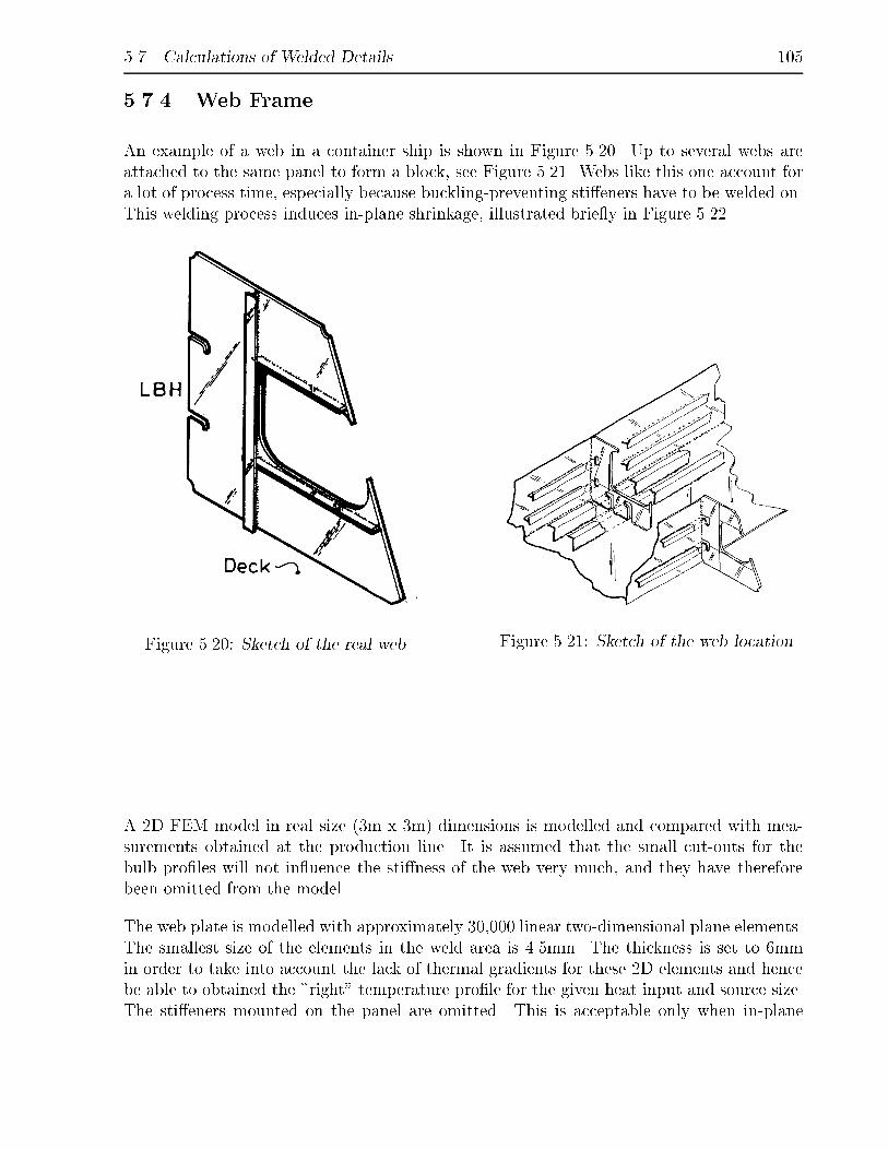
5.7. Calculations of Welded Details 105
5.7.4 Web Frame
An example of a web in a container ship is shown in Figure 5.20. Up to several webs areattached to the same panel to form a block, see Figure 5.21. Webs like this one account fora lot of process time, especially because buckling-preventing sti�eners have to be welded on.This welding process induces in-plane shrinkage, illustrated brie y in Figure 5.22.
Figure 5.20: Sketch of the real web. Figure 5.21: Sketch of the web location.
A 2D FEM model in real size (3m x 3m) dimensions is modelled and compared with mea-surements obtained at the production line. It is assumed that the small cut-outs for thebulb pro�les will not in uence the sti�ness of the web very much, and they have thereforebeen omitted from the model.
The web plate is modelled with approximately 30,000 linear two-dimensional plane elements.The smallest size of the elements in the weld area is 4.5mm. The thickness is set to 6mmin order to take into account the lack of thermal gradients for these 2D elements and hencebe able to obtained the "right" temperature pro�le for the given heat input and source size.The sti�eners mounted on the panel are omitted. This is acceptable only when in-plane

106 Chapter 5. Thermomechanical Analysis Using FEM
Figure 5.22: An artist impression of wel-ding distortions.
x
y
z
0
SY
STU
S+ V
2.0 - HP
-UX
-B.10.20 - S
un May 2 12:34:48 1999
Figure 5.23: The triangular web mesh.
shrinkage is considered. So, only the weld lines for the �llets are modelled. The mesh is �nearound these weld lines, and coarse in the far �eld, as shown in Figure 5.23. The model isclamped in the lower left corner, and simply supported in the lower right corner.
The sti�eners are welded at the same time with only a few seconds in starting times in ordernot to have more than one transient inlet at the time. The problem is solved numerically inthe same way as for the T-pro�le, i.e. �rst the thermal and then the mechanical analysis.The heat is applied by use of the moving Gaussian heat source, de�ned by Eq. 5.31. Thesize of the Gausssian surface is 10mm in the front, 35mm in the rear and the transverseextension is 30mm. The power of the heat source is here twice as much as for a single �lletin order to simulate the total heat input for a double sided �llet in one run. In order toget an easier numerical convergence for the thermal calculation the "jumps" for the speci�cheat and conductivity as seen in Figure 5.11 are omitted and then modelled a straight lines.It is assumed that these local e�ects for the materials parameters do not have a signi�cantin uence of the global result, which has seemed to be true.
Figure 5.24 shows the three heat sources 90 secs after start. Two heat sources move alongthe surface in the X-direction and one heat source moves along the Y-direction. When theheat sources reach the edge they automatically switch o�, and the temperature in the plateis only changed due to the radiative and convective boundary conditions. Figure 5.25 showsa zoomed view of the isotherms around the heat source travelling along the Y-axis. Theextent of the heat source is relatively small compared with the dimensions of the web plate.The temperature of the web plate after 2 hours is shown in Figure 5.26, and as it can be seenis the web plate not completely homogeneous cooled, due to the relative low heat radiationas a boundary condition as also assumed for the 2D plate.
Figure 5.27 is a displacement plot after cooled down. The upper left corner is (A) shrinks2mm, from -3mm obtained just after welding to -1mm after cooling. The X-displacement forthe left edge gives a camber of approximately 4mm. The lower right corner in the cut-out (B)
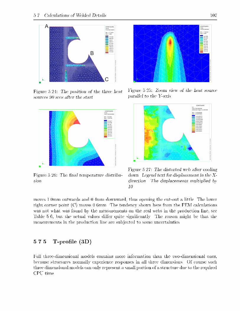
5.7. Calculations of Welded Details 107
Figure 5.24: The position of the three heatsources 90 secs after the start.
x
y
z
0
144.588
1510.26
296.329448.07599.812751.553903.2941055.041206.781358.52
Max = 1662Min = -7.15344 Time 90.000000TempCONTOURS
SY
STU
S+ V
2.0 - HP
-UX
-B.10.20 - M
on May 3 08:24:13 1999
Figure 5.25: Zoom view of the heat sourceparallel to the Y-axis.
x
y
z
0
37.4517
164.605
51.579865.70879.836293.9644108.093122.221136.349150.477
Max = 178.733Min = 23.3235 Time 7200.000000TempCONTOURS
SY
STU
S+ V
2.0 - HP
-UX
-B.10.20 - M
on May 3 08:22:39 1999
Figure 5.26: The �nal temperature distribu-tion.
x
y
z
0
-0.00135073
0.00323869
-0.00084079-0.0003308550.0001790810.0006890160.001198950.001708890.002218820.00272876
Max = 0.00374863Min = -0.00186066 Deformed shape X 10.000000Time 7200.000000Ux
CONTOURS
SY
STU
S+ V
2.0 - HP
-UX
-B.10.20 - M
on May 3 08:33:21 1999
Figure 5.27: The distorted web after coolingdown. Legend text for displacement in the X-direction. The displacements multiplied by10
moves 1.0mm outwards and 0.4mm downward, thus opening the cut-out a little. The lowerright corner point (C) moves 0.6mm. The tendency shown here from the FEM calculationswas not what was found by the measurements on the real webs in the production line, seeTable 5.6, but the actual values di�er quite signi�cantly. The reason might be that themeasurements in the production line are subjected to some uncertainties.
5.7.5 T-pro�le (3D)
Full three-dimensional models contains more information than the two-dimensional ones,because structures normally experience responses in all three dimensions. Of course suchthree dimensional models can only represent a small portion of a structure due to the requiredCPU time.

108 Chapter 5. Thermomechanical Analysis Using FEM
Table 5.6: Shrinkage comparison for web frame.
Point Ux (mm) FEM Ux (mm) MeasurementA Upper left corner -1.0 6B Lower cut-out point 1.0 0.5C Lower right corner 0.6 -0.2
x y
z
0
SY
SW
ELD
+ V 2.0 - H
P-U
X-B
.10.20 - Tue Mar 2 13:16:14 1999
Figure 5.28: The mesh, containing of three and four noded solid, elements used forthe analysis.
Straight Symmetric Pro�le
The T-pro�le considered above is also analysed by a 3D FEM model. The FEM model useslinear triangular and quadratic solid elements with 6 and 8 nodes, respectivily. This kind ofelements has a rather low degree of freedom, but gives a good compromise between accuracyand model size. The materials properties are as those of previous analysis.
The model contains 8165 nodes and 11427 elements. The e�ect of the weld bead geometryhas to be taken into account. It is modelled as a triangular "beam", implemented in theoverall model. The mesh is shown in Figure 5.28. As illustrated in Figure 5.28 the meshdensity increases towards the weld bead which has the highest gradients. The �nest mesh

5.7. Calculations of Welded Details 109
density along the weld bead is 4mm per element.
The heat source is rotated 450 around the longitudinal axis, in order to get a position whichis normal to the bead. The heat source, Q000 expressed by Eq. 2.50, travels from one endto the other. When passing the �nal edge, the heat source turns o� and the pro�le is onlyin uenced by the radiative and convective boundary conditions.
The heat input for the source distribution is corrected by a factor of four in order to achievethe right temperature level in and around the weld bead. In a weld the thermal power isused mainly to melt the �ller material, surrounded by shielding gasses which works as aninsulator for incoming oxides etc. but also as a insulator for outgoing heat. In the FEM casewhere the bead elements are heated up and the heat is conducted to the adjacent elements itis therefore necessary to add a higher heat input to compensate for the heat conditions. InFigure 5.29 the �ne mesh density around the weld bead is included just after the transientinlet. Figure 5.30 shows the quasi-steady state of the heatsource, here depicted after 5secs.
xy
z
0
154.296
1459.78
299.35444.403589.456734.509879.5631024.621169.671314.72
Max = 1604.83Min = 9.24297 Time 1.500000TempCONTOURS
SY
STU
S+ V
2.0 - HP
-UX
-B.10.20 - M
on May 3 09:32:48 1999
Figure 5.29: The temperature distributionaround the heat source, just after the tran-sient inlet.
xy
z
0
161.134
1535.33
313.823466.512619.201771.89924.5781077.271229.961382.64
Max = 1688.02Min = 8.44544 Time 5.000001TempCONTOURS
SY
STU
S+ V
2.0 - HP
-UX
-B.10.20 - M
on May 3 09:35:21 1999
Figure 5.30: The temperature distributionaround the heat source, after 5 secs.
Figure 5.31 shows the reaction of the plate to the heat source 30 secs after the start. Whenthe torch moves at a velocity of 7mm/s, the torch has covered a distance of 210mm. Figure5.32 shows the temperature of the T-pro�le after cooling.

110 Chapter 5. Thermomechanical Analysis Using FEM
x y
z
0
161.191
1536.62
314.017466.843619.669772.495925.3211078.151230.971383.8
Max = 1689.45Min = 8.36475 Time 30.000082TempCONTOURS
SY
STU
S+ V
2.0 - HP
-UX
-B.10.20 - M
on May 3 09:36:37 1999
Figure 5.31: The temperature distribution around the heat source, 30 secs after theinlet.
x y
z
0
21.6963
35.3398
23.212224.728226.244127.760129.27630.79232.307933.8239
Max = 36.8558Min = 20.1804 Time 2479.999512TempCONTOURS
SY
STU
S+ V
2.0 - HP
-UX
-B.10.20 - M
on May 3 09:37:22 1999
Figure 5.32: The temperature distribution after cooling down.
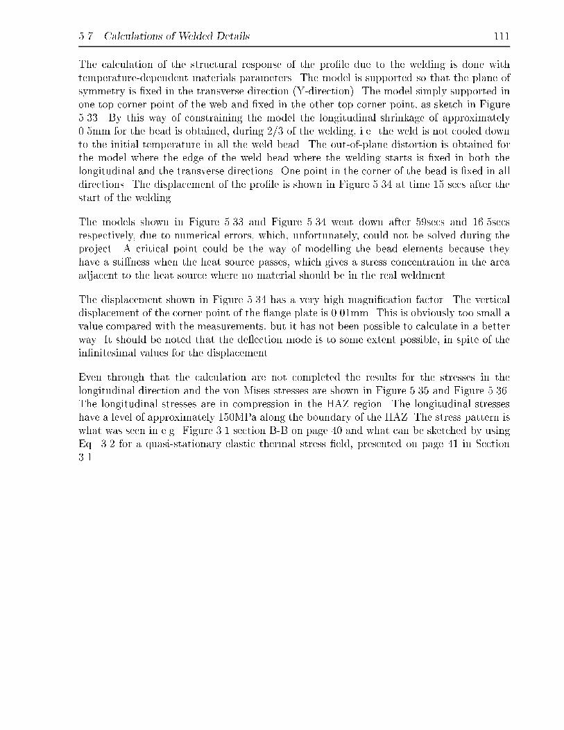
5.7. Calculations of Welded Details 111
The calculation of the structural response of the pro�le due to the welding is done withtemperature-dependent materials parameters. The model is supported so that the plane ofsymmetry is �xed in the transverse direction (Y-direction). The model simply supported inone top corner point of the web and �xed in the other top corner point, as sketch in Figure5.33. By this way of constraining the model the longitudinal shrinkage of approximately0.5mm for the bead is obtained, during 2/3 of the welding, i.e. the weld is not cooled downto the initial temperature in all the weld bead. The out-of-plane distortion is obtained forthe model where the edge of the weld bead where the welding starts is �xed in both thelongitudinal and the transverse directions. One point in the corner of the bead is �xed in alldirections. The displacement of the pro�le is shown in Figure 5.34 at time 15 secs after thestart of the welding.
The models shown in Figure 5.33 and Figure 5.34 went down after 59secs and 16.5secsrespectively, due to numerical errors, which, unfortunately, could not be solved during theproject. A critical point could be the way of modelling the bead elements because theyhave a sti�ness when the heat source passes, which gives a stress concentration in the areaadjacent to the heat source where no material should be in the real weldment.
The displacement shown in Figure 5.34 has a very high magni�cation factor. The verticaldisplacement of the corner point of the ange plate is 0.01mm. This is obviously too small avalue compared with the measurements, but it has not been possible to calculate in a betterway. It should be noted that the de ection mode is to some extent possible, in spite of thein�nitesimal values for the displacement.
Even through that the calculation are not completed the results for the stresses in thelongitudinal direction and the von Mises stresses are shown in Figure 5.35 and Figure 5.36.The longitudinal stresses are in compression in the HAZ region. The longitudinal stresseshave a level of approximately 150MPa along the boundary of the HAZ. The stress pattern iswhat was seen in e.g. Figure 3.1 section B-B on page 40 and what can be sketched by usingEq. 3.2 for a quasi-stationary elastic thermal stress �eld, presented on page 41 in Section3.1.
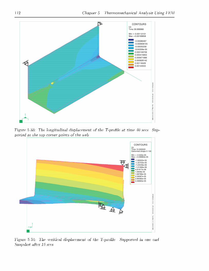
112 Chapter 5. Thermomechanical Analysis Using FEM
Figure 5.33: The longitudinal displacement of the T-pro�le at time 40 secs. Sup-ported at the top corner points of the web.
Figure 5.34: The veritical displacement of the T-pro�le. Supported in one end.Snapshot after 15 secs.

5.7. Calculations of Welded Details 113
x y
z
0
-3.35001e+08
1.79291e+08
-2.77858e+08-2.20714e+08-1.6357e+08-1.06427e+08-4.92832e+077.86038e+066.5004e+071.22148e+08
Max = 2.36435e+08Min = -3.92145e+08 Time 39.999966Sigma 11
CONTOURS
SY
SW
ELD
+ V 2.0 - H
P-U
X-B
.10.20 - Fri May 28 16:47:11 1999
Figure 5.35: The longitudinal stresses around the moving heat source, at time 40secs.
x y
z
0
2.48246e+07
2.48246e+08
4.96492e+077.44738e+079.92984e+071.24123e+081.48948e+081.73772e+081.98597e+082.23421e+08
Max = 2.73071e+08Min = 17.2983 Time 39.999966Von mises stress
CONTOURS
SY
SW
ELD
+ V 2.0 - H
P-U
X-B
.10.20 - Fri May 28 16:47:55 1999
Figure 5.36: The von Mises stresses around the moving heat source, at time 40 secs.
114 Chapter 5. Thermomechanical Analysis Using FEM
This page is intentionally left blank.

Chapter 6
Parametric Expressions and
Veri�cation
6.1 Introduction
The intention of this chapter is to set up some parametric expressions for the shortening andde ection for butt welds and �llets. The majority of the expressions are those which are todayin common use at shipyards - mainly because there is no better alternative. The expressionsare directly or in modi�ed versions compared with measured values at the shipyard and withFE calculations.
For numerical comparisons the two examples listed in Table 6.1 are used.
6.2 Approximate Method for Fillets
Okerblom [41] gives an empirical formula for longitudinal shrinkage and bending, betterknown as sagging, for a �llet weld of a T-pro�le made of low carbon steel.For the curvature (C) and de ection (�) in sagging (camber) the following simpli�ed formulareads
C = 8:4410�7 qz0Iy
(6.1)
The deformation in the middle of a beam due to constant uniform curvature is given by
� = Cl2
8(6.2)
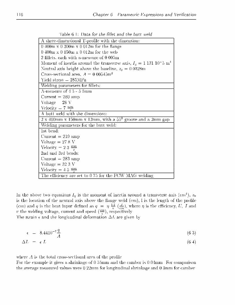
116 Chapter 6. Parametric Expressions and Veri�cation
Table 6.1: Data for the �llet and the butt weld.
A three-dimensional T-pro�le with the dimension:0.400m x 0.300m x 0.012m for the ange.0.400m x 0.150m x 0.012m for the web2 �llets, each with a-measure of 0.005mMoment of inertia around the transverse axis, Iy = 1.131 10�5 m4
Neutral axis height above the baseline, z0 = 0.0328mCross-sectional area, A = 0.00545m2
Yield stress = 285MPaWelding parameters for �llets:A-measure of 4.5 - 5.5mmCurrent = 280 ampVoltage = 28 VVelocity = 7 mm
s.
A butt weld with the dimensions:2 x 400mm x 150mm x 12mm, with a 550 groove and a 2mm gapWelding parameters for the butt weld:1st bead:Current = 219 ampVoltage = 27.8 VVelocity = 2.3 mm
s
2nd and 3rd beads:Current = 283 ampVoltage = 32.3 VVelocity = 4.5 mm
s.
The e�ciency are set to 0.75 for the FCW MAG welding.
In the above two equations Iy is the moment of inertia around a transverse axis (cm4), z0is the location of the neutral axis above the ange weld (cm), l is the length of the pro�le(cm) and q is the heat input de�ned as q = � UI
v( Jcm), where � is the e�ciency, U; I and
v the welding voltage, current and speed ( cms), respectively.
The strain � and the longitudinal deformation �L are given by
� = 8:4410�7q
A(6.3)
�L = � L (6.4)
where A is the total cross-sectional area of the pro�le.For the example it gives a shrinkage of 0.55mm and the camber is 0.04mm. For comparisonthe average measured values were 0.22mm for longitudinal shrinkage and 0.3mm for camber.

6.2. Approximate Method for Fillets 117
For the angular distortion � of the ange due to a single �llet weld Okerblom [41] gives twoformulas:
� = �35:5 10�6 qlin:pen�2
(6.5)
where qlin:pen is the penetration energy ( calcm) de�ned by
qlin:pen =2gflange
2gflange + gweb�mqlin (6.6)
where g is the thickness, �m = 0.43 is a measure of the fraction of the heat used to melt thebase metal, and qlin is the total energy per unit length into the plate.
The second formula reads
� = �64 � 10�3 m
g
!2
(6.7)
where m is the leg length and g the web thickness.
Eq. 6.5 gives an angular deformation of 0.0117 rad which gives corresponds to a verticaldisplacement of 150mm from the rotational centre of 1.76mm. Eq. 6.7 gives an angle of0.0111 rad, which corresponds to a vertical displacement of 1.67mm. The two results agreerather well, also with the measured value of 2.22mm and the 2D FEM value of 1.67mm.
In [30] Lee gives a simple but not very obvious formula for the angular distortion for �llets:
� = �1:2427p1:8943heat e�0:165pheat (10�3rad) (6.8)
where pheat is a heat input parameter de�ned as
pheat =q
g1:5(6.9)
Here g and q are the plate thickness (mm) and the heat input per unit length (cal/mm),respectively.
For the �llet weld example, Eq. 6.8 gives an angular de ection of 0.0147 rad, correspondingto a displacement of 2.2mm 150mm from the centre, exactly as measured.

118 Chapter 6. Parametric Expressions and Veri�cation
Jang [9] proposed a model where it is assumed that the elastoplastic process is concentratedon the circular disc around the heat source. The parametric formula for total angulardistortion (in rad) for the line heating process reads
� = �2(1� �2)1:05
sQ
vg2��
243�0:25Q
4vg2� 2
0:25Q
vg2
!235 (6.10)
where � is the poisson ratio, Q is the strength of the heat source (cal/s), v is the movingspeed of the heat source (mm/s), g the thickness of the plate (mm). The plastic strain �� isde�ned as
�� = �Tc � �y
�1
rK�+1� �dEd
�(6.11)
where � is the thermal expansion of the disc (index d), Tc is the critical temperature hereassumed to be equal to the melting temperature (15300 C), r is the radius of the circulardisc (here equal to 3mm), K� is the spring constant for the plate around the circular disc,K� = Ep
r(1+�p). �y is the yield stress of the disc. By using the same material for the disc and
for the plate Eq. 6.11 becomes
�� = �Tc � �y
�2
E
�(6.12)
In this study it is assumed that the line heating process is comparable with the bead-on-platetest.With �y = 285 MPa and � = 0.3 and on the assumption that the disc material is equal tothe surrounding plate, the angular de ection is 0.020 rad. The displacement is then 3.2mm150mm away from the centre. The value is comparable with the measured ones which areon average 2.2mm.
In [8] Jang presents a formula for the curvature (sagging) of T-pro�les:
C =0:487 �
�cqz0�
1 + 0:487 �Eq�c�yAef
�I
(6.13)
Here � is the thermal expansion coe�cient, ��cis a coe�cient equal to 7.8 10�3 mm3/cal for
steel, Iy is the moment of inertia, z0 is the distance from the neutral axis of the beam tothe heated zone (� 25mm), and Aef is the e�ective area approximately equal to A. By useof Eqs. 6.2 and 6.13 the de ection � for the T-pro�le is calculated to be 0.04mm from theabove formula. The sagging is measured to be 0.3mm for the 400mm long T-specimen. As
6.2. Approximate Method for Fillets 119
in the case of Eq. 6.4 signi�cant deviations from the present measured values occur.
Satoh et al: [54] give some simple expressions for angular distortion (�) and transverseshrinkage (s) for bead-on-plate welding. For mild steel with the welding condition 2500 <qh2� 5000, where q is in cal
cm:
� = �2:4 10�6 qh2
+ 0:021 (rad) (6.14)
s = 1:9 10�5q
h� 0:035h (mm) (6.15)
For the bead-on-plate tests the values are� = 0.026radS = 0.075mmThis angular de ection gives a vertical displacement of 3.9mm 150mm away from the weldline. The measured value is for one bead pass 2.2mm, i.e. somewhat less.
Ueda et al: [63] give a formula for the angular distortion of a T-joint due to �llet welding.The formulas as originally presented by Watanabe and Satoh in 1956read as follows for onepass welding:
� = �0:36
I
(gpvg)
10�3!1:6
exp(�2:8 I
(gpvg)
10�3) (rad) (6.16)
where I is the welding current, v the welding speed in (cm/s), g the plate thickness in cm.For the present example � = 0.020 rad, which gives a displacement of 3mm for the angeside edge, slightly above the measured value of 2.2mm.
White et al: give in [64] an equation for the angular de ection, for a single-pass bead-on-plate weld laid on a long at unclamped plate. The equation is based on experimental resultswhere the plate thickness is the varying parameter and reads
� = 0:22Q
vg2�
180(rad) (6.17)
where q is the power input (W), v the welding speed (mm=s) and g is the thickness of theplate in mm. In the considered case this gives an angle of 0.030 rad. For the edge of the ange this angle results in a displacement of 4.5mm if the welding parameters are as for the�llet weld. A summary of the �ndings is given in Table 6.2.

120 Chapter 6. Parametric Expressions and Veri�cation
Table 6.2: Comparison of di�erent predictions of angular displacement 150mm from the weldfor the T-bar example.
Method De ection [mm]
Measured (present) 2.2FEM (present) 1.7Okerblom [41] 1.8/1.7White [64] 4.5Ueda [63] 3.0Satoh [54] 3.9 (bead-on-plate)Jang [9] 3.2 (line heating)Lee [30] 2.2

Chapter 7
Conclusions and Recommendations
7.1 Conclusion
In the production of ship sections the expenses for rework, such as straightening and adjust-ment work of the modules which are joined together, are an important part of the productioncosts. These inaccuracies arise partly from thermal deformations due to cutting and wel-ding and partly as dimensional variations due to human factors. With the increasing use ofautomatisation, as seen at Odense Steel Shipyard, it is attractive to quantify the thermal de-formations by mathematical models. Thus it would be possible to plan the joining sequencein building up the sections, so that the required tolerances of the sections can be achievedby a minimum of rework.
The objective of the present work has been to investigate and simulate some typical weldingjoints. This included establishing an arbitrary moveable heat source, �nite element models,veri�cation measurements of the temperature distribution in a steel plate and measurementsof distortions and stresses.
When in uence from the welding, i.e. the thermal process, is described and quanti�ed itis possible to simulate the mechanics of the welding process in a computer-based productmodel. In the present work calculations by a �nite element program were performed. Thesimulation routines were applied to a comparison of distortions and stresses of real modelsadopted from the assembly line. These models are both in model size and full-scale size.
Infrared measurements of temperature distribution in di�erent plate thickness', show thatthe overall best assumption about this distribution is that made by Rosenthal, althoughRosenthal's analysis is rather inaccurate for temperatures in or near the heat-a�ected zone.In zones where the temperature is less than half the melting point Rosenthal's solution cangive quite accurate results.

122 Chapter 7. Conclusions and Recommendations
Based on the cooling rates of a weld formulas have been derived in order to determine whethera heat ow for di�erent types of welding and materials parameters, can be calculated as atwo-dimensional or a three-dimensional problem.
Residual strain measurements are made, using strain gauges, on various qualities of steelplates. Large longitudinal residual tensile stresses are produced near the weld fusion line.The magnitude for the residual stresses at the fusion line is 350 MPa for SS400 steel, around500 MPa for low Carbon steel, and 400 MPa for the 9 % Nickel steel. These peak stressesare comparable with the yield stresses for the ground material. A simple procedure forquantitative estimations of residual stresses caused by welding has been outlined using thesectioning method.Slicing up the specimens from the sectioning procedure changes the measured residual stresslevel. The relatively greatest in uence of the slicing is observed where the stress level ishighest.
The rolling direction of a steel plate is shown not to have a signi�cant in uence on the tensilestrength.
In order to illustrate the variation of residual stresses and curvature, a beam theory is used.The resulting permanent curvature is rather small in the calculation made with the simpleplate strip. The elastic bending will results in a hogging mode and the permanent plasticbending is in a slight sagging mode. The residual stress approaches the yield stress atthe neutral axis where the boundary of the unheated material was assumed to be. Thissingularity is not possible in practice, but it illustrates rather well that the highest stresslevel occurs inside the bulk.
Studies have shown that laser welding gives much less in-plane shrinkage, and especiallyout-of-plane distortion, compared with MAG and manual metal arc (electrode) welding.
The traditional handling of welding distortions is not to simulate them but to predict themby empirical rules often in the form of a set of "de ection curves". These curves are afunction of only one or two parameters, and it is often seen that the speci�c parametersavailable are not in the speci�c �gure. Testing of parametric expressions has shown thatthese expressions are relatively precise. The problem is that the parametric expressionsmainly work for standard joints, such as symmetric T-pro�le. In order to make a rationalanalysis of the stresses and distortions in ship sections caused by welding, �nite-elementsimulations are carried out. Simulations which involve non-linear materials parameters andthe thermoelastic-plastic material behaviour law is complied with.
To gain empirical knowledge of the distortions due to welding and to obtain veri�cationdata for the computer simulations, measurements are carried out on some modules in theproduction line and on test specimens in the welding laboratory. Real size longitudinalswelded by use of twin arc shrinks in average 0.33mm/m. The test specimens shows that thecooling rate is rather signi�cant for the shrinkage. Multi-pass welding of the test specimenswill show an elongation after the �rst bead, and then afterward the shrinkage will occur asa function of the following beads. This tendency was obtained by the FEM simulation too.
7.2. Recommendations for Future Work 123
The purpose of the simulation or calculation is to obtain values for in-plane shrinkage andout-of-plane distortion. For the in-plane calculation a plane element model of a plate as-suming a plane stress �eld works quite well. The heat source can be moved in straight linesall over the plate, by use of the developed simpli�ed Fortran subroutine. The start andstop positions, the heat input as power and area or volume, the welding velocity and thepower loss can be speci�ed by the user. The FEM results are here in general lower thanthose experimentally measured. The distortion pattern is as seen in the experiments, whichindicates that this di�erence is just a matter of levelling.
A plane strain model of the cross-section of the symmetric T-pro�le is easy to handle andCPU e�cient. The temperature is here prescribed in the nodes. The heating and coolingcycles are implemented by curves. The results of this kind of analysis show a very highaccuracy between experiments and FEM calculations. A disadvantage of the two-dimensionalmodel is that it cannot take into account complex geometries. Therefore, a three-dimensionalmodel is included too. This model takes into account both the in-plane and out-of planedistortion. The results show no satisfying accuracy but the tendencies are roughly what wasseen from the experiments.
From the experiments it can be stated, that the weld �llet size should be kept at the speci�edminimum, balanced welding about the neutral axis should be used, and that the time betweeneach run should be kept at a minimum.
Computational welding simulations (and mechanics) are not fully established as a sciencebut almost su�ciently developed to be applied to various simpli�ed problems in the shipyardindustry.
The study has shown the advantage of using the FEM for a welding simulation tool, but theobjective of simulating welding distortions in the production line was ambitious, and largethree-dimensional problems have not been solved satisfactorily.
The expected achievements from this kind of projects are at long-term sight
� Improved planning and work scheduling by reducing the rework
� Signi�cant reductions in production costs by reducing the measurements and the re-work
� Improved ship quality
7.2 Recommendations for Future Work
The outlined way of simulating the welding distortions covers the main issues of the non-linear thermoelasto-plastic problem. However, improvements of the FEM models could bemade and additional e�ects could be included.

124 Chapter 7. Conclusions and Recommendations
In the near future much more will be seen of practical applications based on fundamentalmathematics and numerical modelling.
E�ort could be made in the area of welding stresses during phase transformation.
Taking into account the weld �ller material an objective of the theoretical study could beto model, pass by pass, the geometric build-up of the weld as well as the accumulation ofstress and displacement, without having a constraint before the weld passes, i.e. activa-tion/deactivation of elements to simulate welding processes involving the �ller metal.
More attention could be focused on the welding mechanics such as volume changes dueto phase transformation, plasticity transformation, chemical composition and alloy-speci�cmaterials parameters. In the present work the most in uential parameters are taken intoaccount.
A superelement containing a �llet weld with the actual displacements should be the basicelement in building up a more complicated model. The idea is here that a tree-dimensionalstructure can always be broken down in such a �llet element. The elements should be con-nected by springs so that the interaction of the "system" resembles a physical phenomenon.
Modelling the weld bead with solids and then modelling the ange with shells. This methodis called substructuring with superelements.
Further work on the simulation of welding distortion could be done in order to be able totake into account the welding sequence. This involves more elements due to the need of moreweld beads.
In the present work calculations by a �nite element program have been performed. Subse-quently, it should be possible to make corrective preadjustments of geometry and change thejoining process parameters or the joining sequence in order to improve the accuracy in theproduction.
A more comprehensive study could be done in obtaining temperatures inside the bulk of aplate. This could be done by thermo couples, and the challenge here is to get a proper heattransfer from the bulk to the thermo couples.
At last it could be interesting to estimate the probability of defects and the risk of failure ina welding joining process.
7.3 Comments
The purpose of this study has all the time been to produce a "tool" which can simulatethe distortions in a ship section with required precision. The results should mainly help thedesign o�ce to plan the work so unforeseen structural complications due to distortion couldbe redressed already at the design stage.

7.3. Comments 125
7.3.1 Reduction of Welding Distortions
A basic problem here is the fact that welding residual stresses and welding distortion to alarge extent behave in an opposite way. A component which rigidly �xed when welded showshigh residual stresses. If, by contrast, it is welded without any restraint, the distortion islarge and the residual stresses are relatively small. It is therefore not possible in practiceto manufacture a component with both a low level of residual stresses and distortions. Acompromise has often to be made, but in the shipbuilding industry most e�ort is as a rulemade to keep the distortion low, for example by straightening or heating methods.
In general, excessively high temperature concentrations should be avoided, however, not onlybecause of possibly locally increased residual stresses, but because of undesired microstruc-tural changes connected with the temperature gradient over time. Actions concerning thereduction of welding distortion should be arranged according to the design, material andmanufacturing stages.
All wider-ranging decisions, particularly those relating to the groove shape and weldingsequence as well as the choice between continuous and intermittent welds, are assigned tomanufacturing. Of course, also the design engineer has some responsibility, that the weldedstructure is designed so that welding distortion remains controllable during manufacturing.This "idea" of letting every people be responsible for the �nal product does not alwaysconform to organisational commitments.
The principal design and manufacturing measures for limiting welding distortion are
� The smallest possible leg length A-measure
� Intermittent weld
� Transverse welds �rst, longitudinal welds afterwards
� Weld crossings to be avoided by cut-outs
� Overall welding sequence from the centre and outwards
� Quality in all processes
� Tacking as much as possible before welding, no subassemblies
� Prebending of panels for longitudinal welding of girders

126 Chapter 7. Conclusions and Recommendations
7.3.2 Control Needs
As stated in this study, residual stresses and distortion are major problems associated withwelding manufacture of large, complex structures such as those of ships, see also [36]. Com-plex thermal stresses and distortions occur during the welding and residual stresses anddistortions remain, which have various consequences. Most of them are detrimental to theintegrity of welded structures. The shipbuilding industry will face severe problems withresidual stresses and distortion in the years ahead because
� Increasing amounts of thinner sections tend to be more distorted
The best way of dealing with such problems is to develop technologies for controlling andreducing residual stresses and distortion during manufacture.The most e�ective way of reducing distortion is to control the formation of plastic strainsproduced in regions near the weld. The di�culty here is that the necessary control must bemade during welding. If the performed control is correct, the �nal distortion will be reduced.Correct controls consist of
� Prediction capability
� Sensing capability
� Control capability
7.3.3 Expert Systems
It is possible to solve the problem in a reliable way and completely by use of mathematicsand solid mechanics?
This very complex problem, could or should be solved in a team work, not only consisting ofthe design, and manufacturing engineers, but also of the areas of management, policy, science,engineering, techniques and research. Expert knowledge has to be used and productioninformation must be quanti�ed in a user-friendly system. How this could be done is adi�cult task, but relatively new areas as CALS, Concurrent Engineering, Neural Network,Expert Systems, Genetic Algorithm, Fuzzy and Product Data Management are perhapsneedful tools to reach the goal, to control the distortions through the whole production,from plate stack to ship.
The welding residual stresses should be taken into account in the calculation of ship's hullstrength, for the purpose of seeing how the in uence of these stresses a�ects the ship's hullstrength.
7.3. Comments 127
If you stops in getting better,you are no longer good.

128 Chapter 7. Conclusions and Recommendations
This page is intentionally left blank.
Bibliography
[1] Adams, Clyde M. Cooling Rates and Peak Temperatures in Fusion Welding. WeldingJournal, pages 210s{215s, May 1958. Welding Research Supplement.
[2] Anderson, B.A.B. Thermal Stresses in Submerged-Arc Welded Joint Considering PhaseTransformations. Journal of Engineering Materials and Technology, 100:356{362, Oc-tober 1978. Transactions of the ASME.
[3] Benham, P.P., Hoyle, Russel and Ford, Hugh. Thermal Stress. Sir Isaac Pitman & Sons,Ltd., London, 1964.
[4] Birk-S�rensen, M. and Kierkegaard, H. Simulation of Welding Distortions in Theoryand Practice. In ICCAS 97, pages 383{398. Yokohama, Japan, October 1997. Volume2.
[5] Bishop, J.F.W. and Hill, R. A Theory for the Plastic Distortion of a PolycrystallineAggregate under Combined Stress. Philosophical Magazine, 42, 1951.
[6] Boley, Bruno A., Weiner, Jerome H. Theory of Thermal Stresses. John Wiley & Sons,Inc., 1960.
[7] Carslaw, H.S. and Jaeger, J.C. Conduction of Heat in Solids. Clarendon Press, Oxford,second edition, 1988.
[8] Chang, Doo Jang and Seung, Il Seo. Basic Studies for the Automatic Fabrication ofWelded Built-up Beams. Journal of Ship Production, 11(2):111{116, May 1995.
[9] Chang, Doo Jang, Seung, Il Seo and Dae, Eun Ko. A Study on the Prediction ofDeformations of Plates Due to Line Heating Using a Simpli�ed Thermal Elasto-PlasticAnalysis. Journal of Ship Production, 13(1):22{27, February 1997.
[10] Christensen, A.L. Measurements of Stress by X-ray. SAE Information, 1960. Report.TR-182.
[11] Christensen, N., Davies, V. de L. and Gjurmundsen, K. Distribution of Temperaturesin Arc Welding. British Welding Journal, pages 54{75, February 1965.

130 Bibliography
[12] Cook, Robert D., Malkus, Davis S. and Plesha, Michael E. Concepts of Applications ofFinite Element Analysis. John Wiley & Sons, third edition, 1989.
[13] Dezillie, L. Introduction to Thermo-mechanical Changes during Welding. Note fromDept. of Manufacturing Engineering, March 1995. IPT, Lyngby.
[14] EMRC. NISA Manual. User's Manual, Release 6.0, Unix Version, England, 1996.
[15] Floor, Aksel. Creep, Deformations and Stresses. ESAB Denmark Ltd., 2500 Valby, 2ndedition, 1983. Booklet no. 9.
[16] Framatome, Information Systems. SYSTUS+ Analysis Reference Manual, Chapters Ito X, version 1.0. Framasoft + CSI, Paris /Lyon, Frankrig, 1996.
[17] Friedman, E. Thermomechanical Analysis of the Welding Process Using the Finite El-ement Method. Journal Pressure Vessel Technology, 97:206{213, August 1975. Trans-actions of the ASME.
[18] Thomas Gell. Stress Redistribution in Flame - Cut or Welded Thin Plates Subjectedto External Loading. PhD thesis, Chalmers University of Technology, Dept. of MarineStructural Engineering, 1987.
[19] Goldak, J., Gu, Moashi and Karlsson, Lennart. Numerical Aspects of Modeling Welds.ASM Handbook of Welding, 6:1131{1140, 1993.
[20] Goldak, John, Chakravarti, Aditya and Bibby, Malcom. A New Finite Element Modelfor Welding Heat Sources. Metallurgy Transactions B, pages 299{305, June 1984. Vol.15B.
[21] Grong, Oestein. Metallurgical Modelling of Welding. The Institute of Materials, London,1st edition, 1994.
[22] Hansen, Birger. Welding Stresses and Welding Deformations. Svejse Centralen, Copen-hagen, report no. 68.07 edition, 1968. In Danish.
[23] Hansen, H.E., Kjerulf-Jensen, P. and Stempe, Ole B. Varme- og Klimateknik, Grundbog.DANVAK ApS, Teknisk Forlag A/S, K�benhavn, 1990. In Danish.
[24] Heindlhofer, K. Evaluation of Residual Stress. McGraw-Hill Inc., New York, 1948.
[25] Hrivnak, Ivan. Theory of Weldability of Metals and Alloys. Elsevier, Faculty of Metal-lurgy, Technical University Kosice, Czechoslovakia, 1992.
[26] Iwamura, Y and Rybicki, E.F. A Transient Elastic-Plastic Thermal Stress Analysis ofFlame Forming. Journal of Engineering for Industry, February:163{171, 1973.
[27] Iwasaki, Yasuhiro et al. Study on the Forming of Hull Plate by Line Heating Method.Technical Review, Mitsubishi Heavy Industries, Ltd, October:161{170, 1975.
Bibliography 131
[28] Jang, Chang Doo and Seo, Seung ll. A Simpli�ed Method to Estimate LongitudinalDeformations of Built-up Beams Due to Welding and Heating. Journal of Ship Research,39(2):176{183, 1995.
[29] Jog, M.A. , Cohen, I.M. and Ayyaswamy, P.S. Heat Transfer in Electric Arc Welding.Welding and Joining Processes, ASME, 51:135{142, 1991.
[30] Joo-sung, Lee and Gu-gun, Byun. A Study on the Production-oriented Structural DesignInformation System of Panel Blocks. In M.W.C Oosterveld and Tan S.G., editors,Practical Design of Ships and Mobile Units, pages 359{364. Elsevier Science B.V., 1998.
[31] Junek, L., Slov�a�cek, M. and Ochodek, V. Steam Generator Weld Repair and theirIn uence on its Lifetime. In PAM '97 Proceedings, 1997.
[32] Krenk, Steen. Non-linear Analysis with Finite Elements. Dept. of Building Technologyand Structural Engineering, DK-9000 Aalborg University, 1993.
[33] Krutz, G.W. and Segerlind, L.J. Finite Element Analysis of Welded Structures. WeldingResearch Supplement, 57:211s{215s, July 1978.
[34] Malisius, R. Schrumpfungen, Spannungen und Risse beim Schwei�en. Deutscher Verlagf�ur Schweisstechnik (DVS), D�usseldorf, 3. au age edition, 1969. In German.
[35] Masubuchi, Koichi. Analysis of Welded Structures. Massachusetts Institute of Technol-ogy, USA, 1980. Pergamon Press.
[36] Masubuchi, Koichi. Recent M.I.T. Research on Residual Stresses and Distortion inWelded Structures. Journal of Ship Research, 9(3):137{145, 1993.
[37] Masubuchi, Koichi and Martin, D.C. Investigations of Residual Stresses in Steel Weld-ments. Ship Structure Committee, October 1966. SSC-174.
[38] Moshaiov, A. and Latorre, R. Temperature Distribution During Plate Bending by TorchFlame Heating. Journal of Ship Research, 29(1):1{11, March 1985.
[39] Murakawa, Hidekazu. Computational Welding Mechanics and Its Interface with Indus-trial Application. Trans. JWRI, 25(2):191{204, 1996.
[40] Myers, P.S., Uyehara, O.A. and Borman, G.L. Fundamentals of Heat Flow in Welding.Welding Research Council Bulletin, 123, Mechanical Engineering, The University ofWisconsin, Madison, Wis., July 1967.
[41] Okerblom, N.O. The Calculations of Deformations of Welded Metal Structures. Mash-giz, Moscow - Leningrad, 1955.
[42] Osgood, William R. Residual Stresses in Metal Constructions. Reinhold PublishingCo., New York, 1954.
132 Bibliography
[43] Paley, Zvi, Lynch, J.N. and Adams C.M. JR. Heat Flow in Welding Heavy Steel Plate.Welding Research Supplement, pages 71s{79s, February 1964.
[44] Pavelic, V., Tanbakuchi, R., Uyehara, O.A. and Myers, P.S. Experimental and Com-puted Temperature Histories in Gas Tung-sten-Arc Welding. Welding Journal ResearchSupplement, 48:295s{305s, 1969.
[45] Radaj, Dieter. Heat E�ects of Welding. Springer-Verlag, 1992.
[46] Rasmussen, Carsten J. Process Modelling for Automated Multipass GMA-Welding.Master's thesis, Technical University of Denmark, Dept. of Thermal Processing of Ma-terials, August 1996. Appendix.
[47] Rosenthal, D. The Theory of Moving Sources of Heat and Its Application to MetalTreatments. Transactions of A.S.M.E., pages 849{866, November 1946.
[48] Rosenthal, Daniel. Mathematical Theory of Heat Distribution during Welding and Cutting. Welding Journal, 20(5):220s{234s, 1941.
[49] Rykalin, N.N. Calculation of Thermal Processes during Welding. The GovernmentalTechnical Science Publishing Firm for Machine Literature, Moscow, 1951. (In Russian).
[50] Kunihiko Satoh. A note On Heat Conduction by Moving Heat Source. JWRI, 36(2):154{159, 1967. (In Japanese).
[51] Kunihiko Satoh. Handbook on the Strength of Weld Joints. Rikogakusha PublishingCompany, 3rd edition, 1990. (In Japanese).
[52] Satoh, K., Ueda, Y. and Fujimoto, T. Welding Deformations, Residual Inherent Stress.Sanho Syuppan Publishing Company, 1979.
[53] Satoh, Kunihiko and Terasaki, Toshio. E�ect of Welding Condition on Residual StressDistribution and Welding Deformation in Welding. (In Japanese), 1976.
[54] Satoh, Kunihiko and Terasaki, Toshio. E�ect of Welding Conditions on Welding Defor-mations in Welded Structural Materials. JWRI, 1976. Vol. 45, pp. 302.
[55] Systus International, ESI Group. SYSWELD+ c 2.0 Rerefence Manual. ESI Group,Paris /Lyon, France, 1998.
[56] Systus International, ESI Group. SYSWORLD+ Technical Description of Capabilities,ver.2.0. ESI Group, Paris /Lyon, France, 1998.
[57] Systus International, ESI Group. SYSWORLD+ c Analysis Reference Manual, ver.2.0.ESI Group, Paris /Lyon, France, 1998.
[58] Tada, H. and Paris, P.C. The Stress Intensity Factor for a Crack Perpendicular to theWelding Bead. International Journal of Fracture, 21:279{284, 1983.
Bibliography 133
[59] Tvergaard, Viggo. Plasticity and Creep in Structural Material. Department of SolidMechanics, DTU, Denmark, 1997. (In Danish).
[60] Ueda, Yukio and Ma, Ning-Xu. Measuring Methods of Three-Dimensional ResidualStress with Aid of Distribution Functions of Inherent Strain. Transactions of JWRI,24(2), 1995. Japan.
[61] Ueda, Yukio, Fukuda, Keiji, Tanigawa, Masayuki. New Measuring Method of ThreeDimensional Residual Stress Based on Theory of Inherent Strain. Transactions of JWRI,8(2), 1979. Japan.
[62] Ueda, Yukio, Murakawa, Hidekazu, Rashwan, Ahmed M. Neki, Isao, Kamichika, Ry-oichi, Ishiyama, Morinobu and Ogawa Jun-ichiro. Development of Computer-AidedProcess Planning System for Plate Bending by Line Heating (Report 3){Relation Be-tween Heating Condition and Deformation. Journal of Ship Production, 10(4):248{257,1994.
[63] Ueda, Yukio, Nakacho, Keiji, Moriyama, Shuji. Simple Prediction Methods for WeldingDe ection and Residual Stress of Sti�ened Panels. Transactions of JWRI, 15(2), 1986.Japan.
[64] White, J.D., Leggatt, R.H. and Dwight, J.B. Weld Shrinkage Prediction. In BOSS'79,pages 245 { 266, Cran�eld, Bedford, England, 28 to 31 August 1979. BHRA FluidEngineering. Vol. 1, paper 19.

134 Bibliography
This page is intentionally left blank.
Appendix A
Simple FEM Calculation with Strain
Measurements
A.1 FEM-Calculations
The purpose is to demonstrate the possibilities of using a second non-linear FEM programnamed NISATM to simulate the welding process. One of the test samples with one-sided �lletweld is selected for the analysis, which can be split up into two tasks: First the temperaturedistribution is found, and secondly, the non-linear elastic-plastic behaviour of the materialis obtained by use of the temperature distribution. Both tasks can be analysed by the�nite element method, but in order to make a simple FEM-analysis and with as low CPU-time as possible, only the elastic-plastic module of the FEM-program is used in the presentinvestigation. The temperature distribution around the moving heat source is instead takento be the analytical solution for a 2D in�nite plate. Hence, the temperature distributionacross the thickness is not taken into account and therefore the out-of-plane displacement isnot determined.
The NISA program is one of the commercial FEM programs which have been studied duringthe project, in order to �nd the most advantageous program for the actual welding distortionproblem.
A.1.1 The Finite Element Model
Only half of the base plate in the T-sample is modelled in the FE-model, see Figure A.1.The model is, as mentioned earlier, analysed by the non-linear FEM-package NISATM [14].
The model is a plane model where a symmetry condition is applied to the centre of the baseplate, i.e. Uy = Rx = Rz = 0 at the lower edge. The model is �xed in the x-direction at the
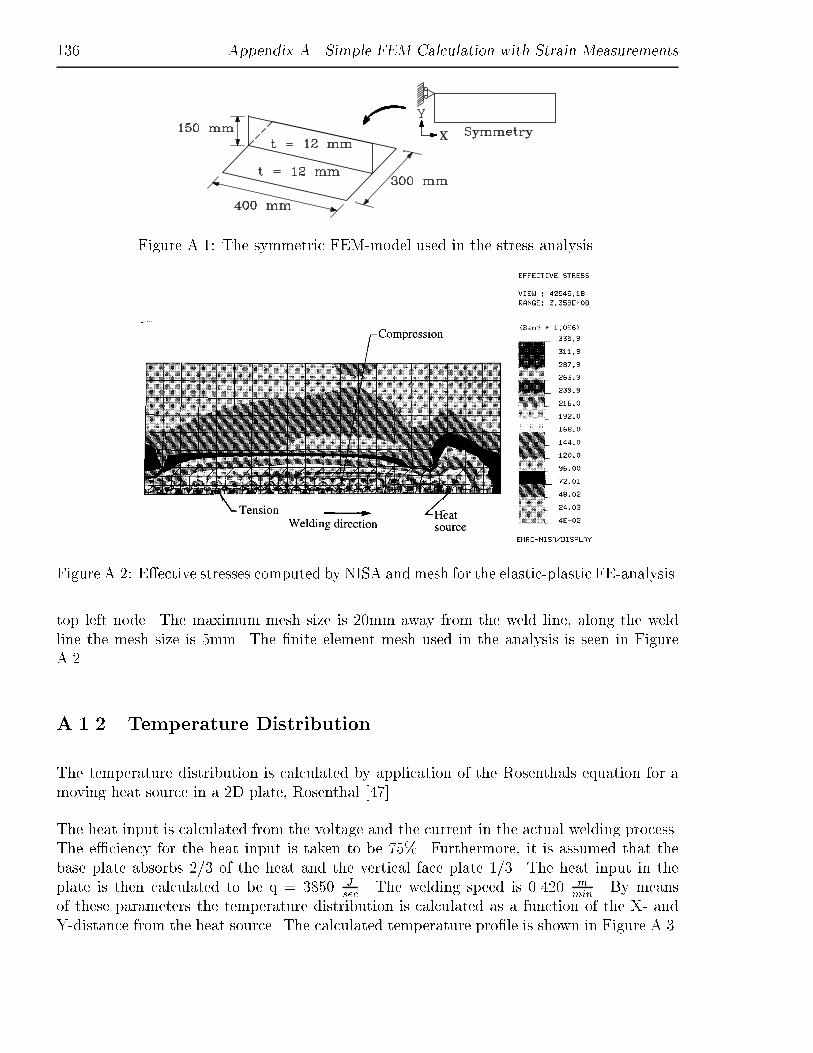
136 Appendix A. Simple FEM Calculation with Strain Measurements
Figure A.1: The symmetric FEM-model used in the stress analysis.
Figure A.2: E�ective stresses computed by NISA and mesh for the elastic-plastic FE-analysis.
top left node. The maximum mesh size is 20mm away from the weld line, along the weldline the mesh size is 5mm. The �nite element mesh used in the analysis is seen in FigureA.2.
A.1.2 Temperature Distribution
The temperature distribution is calculated by application of the Rosenthals equation for amoving heat source in a 2D plate, Rosenthal [47].
The heat input is calculated from the voltage and the current in the actual welding process.The e�ciency for the heat input is taken to be 75%. Furthermore, it is assumed that thebase plate absorbs 2=3 of the heat and the vertical face plate 1=3. The heat input in theplate is then calculated to be q = 3850 J
sec. The welding speed is 0.420 m
min. By means
of these parameters the temperature distribution is calculated as a function of the X- andY-distance from the heat source. The calculated temperature pro�le is shown in Figure A.3.
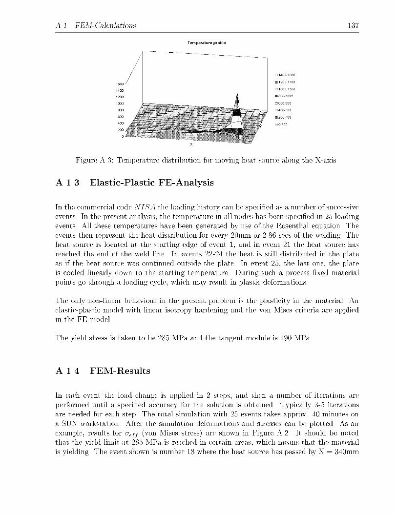
A.1. FEM-Calculations 137
Figure A.3: Temperature distribution for moving heat source along the X-axis.
A.1.3 Elastic-Plastic FE-Analysis
In the commercial code NISA the loading history can be speci�ed as a number of successiveevents. In the present analysis, the temperature in all nodes has been speci�ed in 25 loadingevents. All these temperatures have been generated by use of the Rosenthal equation. Theevents then represent the heat distribution for every 20mm or 2.86 secs of the welding. Theheat source is located at the starting edge of event 1, and in event 21 the heat source hasreached the end of the weld line. In events 22-24 the heat is still distributed in the plateas if the heat source was continued outside the plate. In event 25, the last one, the plateis cooled linearly down to the starting temperature. During such a process �xed materialpoints go through a loading cycle, which may result in plastic deformations.
The only non-linear behaviour in the present problem is the plasticity in the material. Anelastic-plastic model with linear isotropy hardening and the von Mises criteria are appliedin the FE-model.
The yield stress is taken to be 285 MPa and the tangent module is 490 MPa.
A.1.4 FEM-Results
In each event the load change is applied in 2 steps, and then a number of iterations areperformed until a speci�ed accuracy for the solution is obtained. Typically 3-5 iterationsare needed for each step. The total simulation with 25 events takes approx. 40 minutes ona SUN workstation. After the simulation deformations and stresses can be plotted. As anexample, results for �eff (von Mises stress) are shown in Figure A.2. It should be notedthat the yield limit at 285 MPa is reached in certain areas, which means that the materialis yielding. The event shown is number 18 where the heat source has passed by X = 340mm
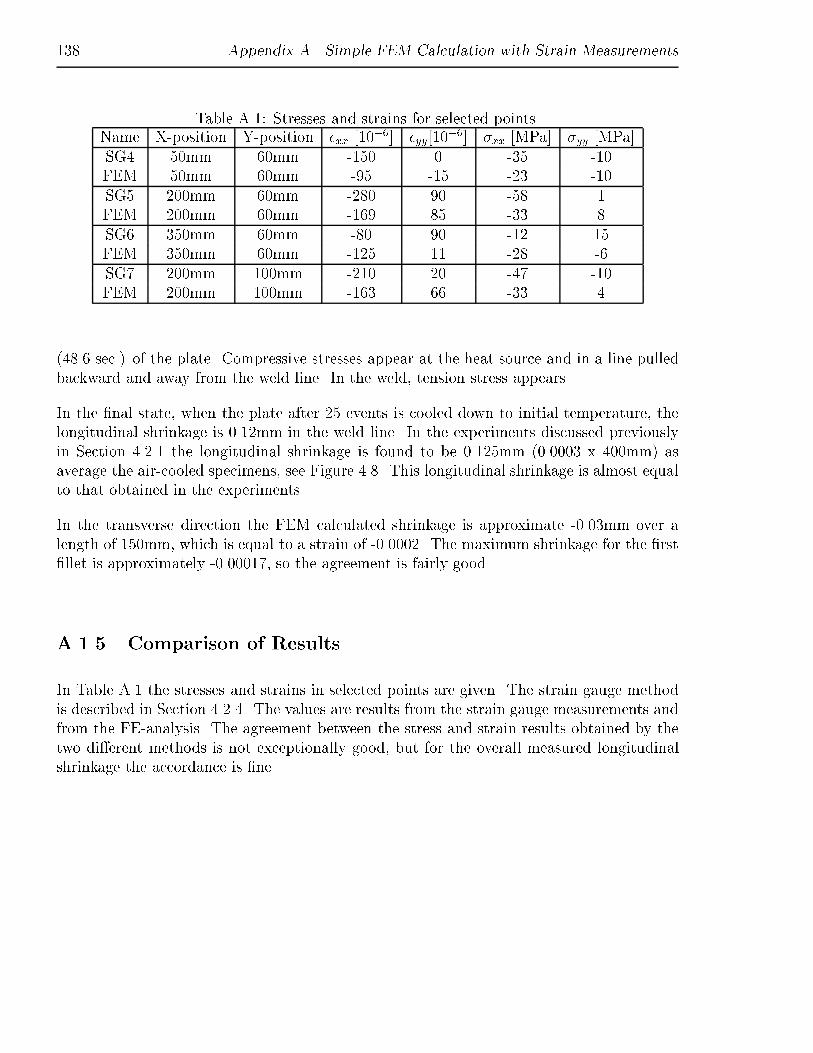
138 Appendix A. Simple FEM Calculation with Strain Measurements
Table A.1: Stresses and strains for selected points.Name X-position Y-position �xx [10
�6] �yy[10�6] �xx [MPa] �yy [MPa]
SG4 50mm 60mm -150 0 -35 -10FEM 50mm 60mm -95 -15 -23 -10SG5 200mm 60mm -280 90 -58 1FEM 200mm 60mm -169 85 -33 8SG6 350mm 60mm -80 90 -12 15FEM 350mm 60mm -125 11 -28 -6SG7 200mm 100mm -210 20 -47 -10FEM 200mm 100mm -163 66 -33 4
(48.6 sec.) of the plate. Compressive stresses appear at the heat source and in a line pulledbackward and away from the weld line. In the weld, tension stress appears.
In the �nal state, when the plate after 25 events is cooled down to initial temperature, thelongitudinal shrinkage is 0.12mm in the weld line. In the experiments discussed previouslyin Section 4.2.1 the longitudinal shrinkage is found to be 0.125mm (0.0003 x 400mm) asaverage the air-cooled specimens, see Figure 4.8. This longitudinal shrinkage is almost equalto that obtained in the experiments.
In the transverse direction the FEM calculated shrinkage is approximate -0.03mm over alength of 150mm, which is equal to a strain of -0.0002. The maximum shrinkage for the �rst�llet is approximately -0.00017, so the agreement is fairly good.
A.1.5 Comparison of Results
In Table A.1 the stresses and strains in selected points are given. The strain gauge methodis described in Section 4.2.4. The values are results from the strain gauge measurements andfrom the FE-analysis. The agreement between the stress and strain results obtained by thetwo di�erent methods is not exceptionally good, but for the overall measured longitudinalshrinkage the accordance is �ne.

Appendix B
An Example of a Data �le
B.1 Introduction
The SYSWORLD software can be run in both the interactive mode and by use of input�les. The latter is the easiest to handle because the options are well arranged, and thus theaccess to options, properties precessions etc. are easy to change. The included �le is withthe moving heat source and radiative boundary condition.
B.2 The SYSWORLD Data File
search data 11
;*********************File 3DT.DAT****************************************
;This file is the one used for moving heat source (Gauss bell) on a 3D T profile
;**************************************************************************
MODE BATCH
DEFINITION
one moving heat sources
OPTION THERMAL SPATIAL
RESTART GEOM
MATE PROP
ELEM 1 to 34080 / KX KY KZ -1 RO 7850 C -2 INTEG 2
CONSTRAINTS
ELEM 34081 to 38510 / KT 1 vari 6
LOADING
1
ELEM 1 to 34080 / QR 1 vari -3
ELEM 34081 to 38510 / tt 20

140 Appendix B. An Example of a Data �le
TABLE
; conductivity KX=KY=KZ=f(T) [W/(m k)]
1 / 1 0 41 200 41 400 38 600 32 870 26 1470 32 1600 230
; specific heat C=f(T) [J/(kg K)]
2 / 1 0 350 580 750 700 900 750 900 810 800 875 620
1510 750 1530 2500 1550 750
3 / FORTRAN
FUNCTION F(X)
DIMENSION X(5)
; Co-ordinates of Gauss point under consideration
xx = X(1)
yy = X(2)
zz = X(3)
t = X(4) ; current time value
; del = 0 ; Delay time
; t = t- del ; t- delay time
if(t.lt.0) goto 35
; Source data
q0=0
; **INPUT*PRIMARY*Source 1**********************
; U = 28 ; Voltage [V] *
; I = 280 ; Current [Amp] *
; eta = 0.75 ; Efficiency [-] *
; Velocity of source
v=0.007 ; m/s
; START coordinates for the heat source
xs=0.0
ys=0.01
zs=0.0035
; STOP co-ordinates for the heat source
xst=0.4
yst=0.01
zst=0.0035
; **INPUT SECONDARY(ellipsoid parameters)******
; a1 = 0.005 ; semiaxis- in translation direction (in front)[m]
; a2 = 0.010 ; semiaxis in translation direction (behind) [m]
; b = 0.020 ; semiaxis in transverse direction [m]
; c = 0.025 ; depth of energy flux [m]
; ff = 0.8
; fr = 1.2
; pi = 3.141593
; **END of INPUT*******************************
; q = U * I
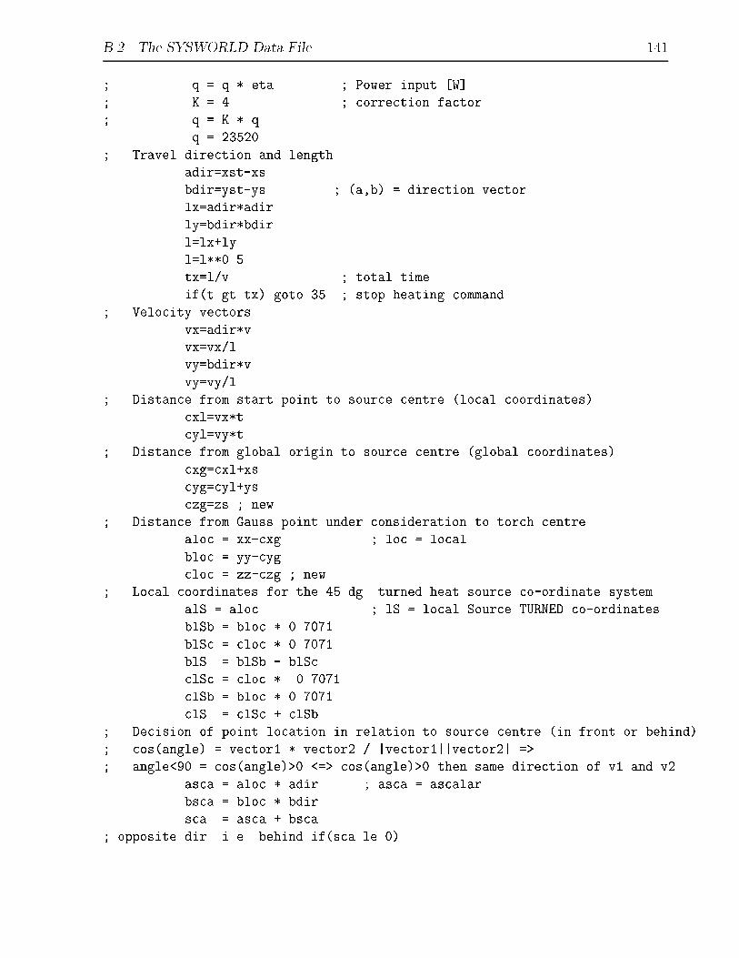
B.2. The SYSWORLD Data File 141
; q = q * eta ; Power input [W]
; K = 4 ; correction factor
; q = K * q
q = 23520
; Travel direction and length
adir=xst-xs
bdir=yst-ys ; (a,b) = direction vector
lx=adir*adir
ly=bdir*bdir
l=lx+ly
l=l**0.5
tx=l/v ; total time
if(t.gt.tx) goto 35 ; stop heating command
; Velocity vectors
vx=adir*v
vx=vx/l
vy=bdir*v
vy=vy/l
; Distance from start point to source centre (local coordinates)
cxl=vx*t
cyl=vy*t
; Distance from global origin to source centre (global coordinates)
cxg=cxl+xs
cyg=cyl+ys
czg=zs ; new
; Distance from Gauss point under consideration to torch centre
aloc = xx-cxg ; loc = local
bloc = yy-cyg
cloc = zz-czg ; new
; Local coordinates for the 45 dg. turned heat source co-ordinate system.
alS = aloc ; lS = local Source TURNED co-ordinates
blSb = bloc * 0.7071
blSc = cloc * 0.7071
blS = blSb - blSc
clSc = cloc * 0.7071
clSb = bloc * 0.7071
clS = clSc + clSb
; Decision of point location in relation to source centre (in front or behind)
; cos(angle) = vector1 * vector2 / |vector1||vector2| =>
; angle<90 = cos(angle)>0 <=> cos(angle)>0 then same direction of v1 and v2
asca = aloc * adir ; asca = ascalar
bsca = bloc * bdir
sca = asca + bsca
; opposite dir. i.e. behind if(sca.le.0)

142 Appendix B. An Example of a Data �le
; same direction i.e. in front if(sca.gt.0)
a = 0.01; a2
fs = 1.2; fr
if(sca.gt.0) a = 0.005; a1
if (sca.gt.0) fs = 0.8 ; fs = ff
; q = ((6*sqrt(3)f*Q/a*b*c*pi*sqrt(pi)) *exp(-3*x**2/a**2)*exp(-3*y**2/b**2)
; *exp(-3*z**2/c**2)
30 EE1= 6
EE1= 1.732 * EE1
EE1= fs * EE1
EE1=q * EE1
EE2=a * 0.020 ; b
EE2=EE2 * 0.025 ; c
EE2=EE2 * 5.568 ; pi * sqrt(pi)
EE4=EE1 / EE2
; 1st exp. function
EX1=alS
EX1=EX1**2
EX1=3 * EX1
EX1=-EX1
EX2=a * a
EX3=EX1 / EX2
EXX=exp(EX3)
; 2nd exp. function
EY1=blS
EY1=EY1**2
EY1=3 * EY1
EY1=-EY1
EY2=0.020 * 0.020 ;b * b
EY3=EY1 / EY2
EXY=exp(EY3)
; 3rd exp. function
EZ1=clS
EZ1=EZ1**2
EZ1=3 * EZ1
EZ1=-EZ1
EZ2=0.025 * 0.025 ;c * c
EZ3=EZ1 / EZ2
EXZ=exp(EZ3)
; summing up
EE=EXX * EXY
EE=EE * EXZ
EE=EE * EE4
; limit for distribution

B.2. The SYSWORLD Data File 143
ELIM=EE*0.1
if(EE.le.ELIM) EE=0
; power function f(x)
F=EE + q0
goto 40
35 F=q0
40 continue
return
end
;***************************
6 / FORTRAN
FUNCTION F(T)
; Radiation losses
; F = SIG * EPS * (T+T0)*(T$^2$ + T0$^2$)
EPS = 0.7
SIG = 5.678*-8
T0 = 20
A = 0
; Temperature in Kelvin degrees
T0 = T0 + 273.15
T1 = T + 273.15
; Calculation of losses by radiation
A = T1 * T1
B = T0 * T0
C = A + B
D = T1 + T0
D = D * C
D = D * EPS
D = D * SIG
; Losses by convection
; Assumption 25 W/m$^2$
; Total losses
F = D + 25
CONTINUE
RETURN
END

144 Appendix B. An Example of a Data �le
RETURN
TRANS NON-LINEAR
RENUMBER
ALGO BFGS ITERATION 20 CORRECTION 10
METHOD ITER
PRECISION ABSO DISPLACEMENT 10
INIT COND
NODES / tt = 20
TIME INIT 0
0.02 step 0.005 / store 1 ; 4
0.06 step 0.01 / store 1 ; 4
0.1 step 0.02 / store 1 ; 2
5.0 step 0.05 / store 1 ; 98
40.0 step 0.1 / store 1 ; 350
300.0 step 10 / store 1 ; 26
3600 step 100 / store 1 ; 33
RETURN
MODE INTE
SAVE DATA TRAN 2
;****************END OF THERMAL COMPUTATION***************
;****************mechanical computations***************
SEARCH DATA 11
MODE BATCH
DEFINITION
MECHANICAL COMPUTATION
OPTION THREE DIMENSIONAL THERMOPLAST
RESTART GEOMETRY
MATERIALs PROPERTIES
E / E -1 NU -2 LX LY LZ -3 YIELD -4 SLOPE -5 MODEL 3 INTEG 2
CONSTRAINT
PLANE NODE 1 12 10524 / UY=0
PLANE NODE 10522 10524 21031 / UY=0
NODE 21020 / UY=UZ=0
NODE 1 / UX=UY=UZ=0
LOADING
1 Thermomechanical statements
TABLE
; Young's modulus [Pa]
1 / 1 20 210000*6 100 203000*6 200 198000*6 300 190000*6 400 180000*6
500 166000*6 600 137000*6 650 105000*6 700 82000*6 750 64000*6
800 52000*6 850 42000*6 900 33000*6 1000 20000*6
1100 1000*6 1250 10*6 1600 1*2

B.2. The SYSWORLD Data File 145
; Poisson's ratio [-]
2 / 1 0 0.28 400 0.3 1500 0.49
; Thermal expansions coef.
3 / 1 20 1.2*-5 1250 0.01845*-3
; Yield stress
4 / 1 20 285*6 400 250*6 700 40*6 1000 15*6 1600 1*2
5 / 7 20 11 400 12 700 13 1000 14 1600 15
11 / 1 0 285*6 1 1050*6
12 / 1 0 250*6 1 1200*6
13 / 1 0 40*6 1 130*6
14 / 1 0 15*6 1 55*6
15 / 1 0 1*2 1 1*3
RETURN
mode inte
SAVE DATA 3
ASSI 19 TRAN2.TIT BINA
TEMPERATURE TRANSIENT CARD 1 to 517
DEASSIGN 19
TRANS NON LINEAR STATIC
RENUMBER
BEHAVIOUR PLASTIC UPDATE
ALGO BFGS ITER 20 CORRECTION 10
METHOD ITERATIVE
PRECISION ABSOLUTE DISPLACEMENT 0.000005; FORCE 0.000001
TIME INITIAL 0
0.02 step 0.005 / store 4 ; 1
0.06 step 0.01 / store 4 ; 1
0.1 step 0.02 / store 2 ; 1
5.0 step 0.02 / store 245; 1
40.0 step 0.1 / store 350; 1
300 step 10 / store 26 ; 1
3600 step 100 / store 33 ; 1
RETURN
SAVE DATA TRAN 4

146 Appendix B. An Example of a Data �le
This page is intentionally left blank
Ph.D. ThesesDepartment of Naval Architecture and O�shore Engineering
Technical University of Denmark � Lyngby
1961 Str�m-Tejsen, J. Damage Stability Calculations on the Computer DASK.
1963 Silovic, V. A Five Hole Spherical Pilot Tube for three Dimensional Wake Measure-ments.
1964 Chomchuenchit, V. Determination of the Weight Distribution of Ship Models.
1965 Chislett, M.S. A Planar Motion Mechanism.
1965 Nicordhanon, P. A Phase Changer in the HyA Planar Motion Mechanism andCalculation of Phase Angle.
1966 Jensen, B. Anvendelse af statistiske metoder til kontrol af forskellige eksisterendetiln�rmelsesformler og udarbejdelse af nye til bestemmelse af skibes tonnage og sta-bilitet.
1968 Aage, C. Eksperimentel og beregningsm�ssig bestemmelse af vindkr�fter p�a skibe.
1972 Prytz, K. Datamatorienterede studier af planende b�ades fremdrivningsforhold.
1977 Hee, J.M. Store sideportes ind ydelse p�a langskibs styrke.
1977 Madsen, N.F. Vibrations in Ships.
1978 Andersen, P. B�lgeinducerede bev�gelser og belastninger for skib p�a l�gt vand.
1978 R�omeling, J.U. Buling af afstivede pladepaneler.
1978 S�rensen, H.H. Sammenkobling af rotations-symmetriske og generelle tre-dimen-sionale konstruktioner i elementmetode-beregninger.
1980 Fabian, O. Elastic-Plastic Collapse of Long Tubes under Combined Bending andPressure Load.
1980 Petersen, M.J. Ship Collisions.
1981 Gong, J. A Rational Approach to Automatic Design of Ship Sections.
1982 Nielsen, K. B�lgeenergimaskiner.
1984 Rish�j Nielsen, N.J. Structural Optimization of Ship Structures.
1984 Liebst, J. Torsion of Container Ships.
1985 Gjers�e-Fog, N. Mathematical De�nition of Ship Hull Surfaces using B-splines.
148 List of Ph.D. Theses Available from the Department
1985 Jensen, P.S. Station�re skibsb�lger.
1986 Nedergaard, H. Collapse of O�shore Platforms.
1986 Junqui, Y. 3-D Analysis of Pipelines during Laying.
1987 Holt-Madsen, A. A Quadratic Theory for the Fatigue Life Estimation of O�shoreStructures.
1989 Vogt Andersen, S. Numerical Treatment of the Design-Analysis Problem of ShipPropellers using Vortex Lattice Methods.
1989 Rasmussen, J. Structural Design of Sandwich Structures.
1990 Baatrup, J. Structural Analysis of Marine Structures.
1990 Wedel-Heinen, J. Vibration Analysis of Imperfect Elements in Marine Structures.
1991 Almlund, J. Life Cycle Model for O�shore Installations for Use in Prospect Eval-uation.
1991 Back-Pedersen, A. Analysis of Slender Marine Structures.
1992 Bendiksen, E. Hull Girder Collapse.
1992 Buus Petersen, J. Non-Linear Strip Theories for Ship Response in Waves.
1992 Schalck, S. Ship Design Using B-spline Patches.
1993 Kierkegaard, H. Ship Collisions with Icebergs.
1994 Pedersen, B. A Free-Surface Analysis of a Two-Dimensional Moving Surface-Pierc-ing Body.
1994 Friis Hansen, P. Reliability Analysis of a Midship Section.
1994 Michelsen, J. A Free-Form Geometric Modelling Approach with Ship Design Ap-plications.
1995 Melchior Hansen, A. Reliability Methods for the Longitudinal Strength of Ships.
1995 Branner, K. Capacity and Lifetime of Foam Core Sandwich Structures.
1995 Schack, C. Skrogudvikling af hurtigg�aende f�rger med henblik p�a s�dygtighed oglav modstand.
1997 Cerup Simonsen, B. Mechanics of Ship Grounding.
1997 Riber, H.J. Response Analysis of Dynamically Loaded Composite Panels.
1997 Olesen, N.A. Turbulent Flow past Ship Hulls.

List of Ph.D. Theses Available from the Department 149
1998 Andersen, M.R. Fatigue Crack Initiation and Growth in Ship Structures.
1998 Nielsen, L.P. Structural Capacity of the Hull Girder.
1999 Zhang, S. The Mechanics of Ship Collisions.


Department of Naval Architecture
And Offshore Engineering
Technical University of Denmark
Building 101E
Dk-2800 Lyngby
Denmark
Phone +45 4525 1360
Telefax +45 4588 4325
Internet
[email protected]://www.ish.dtu.dk
ISBN 87-89502-13-2
Related Documents


