Simulation of the transient behavior of fuel cells by using operator splitting techniques for real-time applications

1

Simulation of the transient behavior of fuel cells by using operator splitting

techniques for real-time applications

Ákos Kriston*1, György Inzelt

1, István Faragó

2, Tamás Szabó

2

1Department of Physical Chemistry, Institute of Chemistry, Eötvös Loránd University,

1117 Budapest,Pázmány Péter sétány 1/a, Hungary

2Department of Applied Analysis and Computational Mathematics, Eötvös Loránd University,

P.O. Box 120, H-1518 Budapest, Hungary

*e-mail: [email protected]

Abstract

The functioning of fuel cells, in which simultaneous processes having different kinetics and different time

constants occur, can be simulated by applying rather complex models. For the sake of better modeling

larger numbers of sub-processes and their couplings have to be considered, which leads to complex and

multi-step simulation frameworks. In this work new methods are introduced for the simulation of the

behavior of fuel cells, which are based on operator splitting techniques. These methods can be applied for

the simulation of rather complex problems, consequently they open up new vistas in respect to the real-

time simulation. The errors of the schemes are analyzed while applying different kinetic approaches. The

effects of constant current, current sweep and pulsed current are calculated. The qualitative and

quantitative errors are analyzed and compared with measured data. It is proven that the method developed

is suitable for describing the fast transient behavior, therefore it makes the real-time monitoring and

controlling of the functioning of fuel cells possible.

Keywords: fuel cell, real-time simulation, operator splitting, pulsed load, peak power,

FPGA

2

1 Introduction

The importance of modeling analyses of fuel cells is threefold. First, it leads to a better

understanding of the underlying phenomena. Second, it provides a useful tool for the

optimization of fuel cell systems. Third, it will be crucial to control FC based

applications (vehicle, backup power etc.) in the future. The general method to build up a

reliable model starts with the selection of the phenomena that primarily influence FC‟s

performance under interest. The subsequent step is the description of these processes in

terms of differential or algebraic equations, and finally the selection of an adequate

mathematical scheme. The use of an analytical method leads to an exact description,

however, it can be applied only for very simplified cases. A broadly used empirical

model was published by Kim et al. [1], which fits the experimental curves excellently,

but without the detailed interpretation of the parameters used. This model can be applied

for the steady-state behavior of fuel cells [2] and for real-time simulation, but it is

unsuitable for the optimization of the parameters, like Pt loading, Nafion content etc.

The transient behavior cannot be elucidated by this model, either.

Gomadam et al. [3] studied the transient behavior of porous electrodes by using a

linearized form of the kinetic equations related to the electrochemical reactions. The

double-layer effect was also taken into account. The respective set of partial differential

equations (PDEs) has been solved analytically. Based on the results of the calculation

the corresponding impedance spectra were derived for different configurations of the

measurement. Because of using linear relationship, the steady-state performance in the

whole current range cannot be interpreted. Kulikovsky [4] gave two asymptotic

solutions for high and low currents, respectively, assuming ideal transport of reactants.

By the expressions derived for voltage-current curves, the appearance of the double

3

Tafel slope was elucidated. Other asymptotic solutions were given by Jaounen [5] for

the voltage–current curves considering the structure of the electrode, by using a

spherical agglomerate model. Deeper insight and understanding of the effects of the

material parameters for fuel cell performance can be achieved by the exact expressions,

however, the detailed and transient behaviors cannot be predicted by analytical models.

Results obtained by numerical models are less general, but both the steady-state voltage

–current curves (V-I curves) and transient effects can be interpreted. These methods can

be used for parameter estimation of the transport and electrochemical properties [6], and

they are also useful for revealing new parameter‟s effects [7]. Complex models [8] are

needed to solve different phenomenological equations such as the Nernst-Planck

equation for multiple mass transport, the Stefan-Maxwell equation for heat transfer,

Ohm‟s law for ionic migration and electron conductivity, and the equations of

electrochemical kinetics. These transport and transfer processes are coupled, and the

equations are often highly nonlinear. In practical systems (using real parameters) these

processes have different time scales, as well. However, each of the subsystems requires

different numerical schemes with different time and spatial discretizations. These

models are usually solved by using only a single numerical treatment e.g., Runge-Kutta,

Newton or Cranck-Nicholson methods. The solution of the respective numerical scheme

is quite slow (sometimes slower than an experiment), therefore this type of techniques

for real-time simulation cannot be applied. There are some possibilities for reducing the

running time. For instance, Faragó et al. developed a parameter scaling method [9], with

the help of which the parameter set of the original problem is converted to a more stable

space and after the execution of the calculation the results are transformed back by

using a reverse transformation. The stability of the scheme substantially increased and

4

the time required to calculate the results decreased by 10000 times, while the error of

the calculation was less than 5%.

Subramanian [10] et al. developed a method to reduce the number of the governing

partial algebric equations (PAEs) of Li-ion battery simulation by using different

mathematical techniques (Ljapunov-Schmidt, volume averaging, dimension analysis

etc). The original problem with a proper discretization has 4800 PAEs which can be

reduced to 49, and finally the simulation time of the discharge curve can be cut to 85

ms. However, in this model the double-layer capacitance was not included. The

completion of the model with the capacitance the simulation of transient behavior

would certainly increase the duration of the execution.

It is quite evident that there is no such method which fulfills all of the requirements.

Therefore, in this work a new numerical method, the operator splitting technique [11] is

applied for the simulation of fuel cells. The procedure applied herein possesses

practically all of the advantages of the other techniques mentioned previously, i.e.,

dealing with complexity, using different numerical schemes and its characteristic

properties. Furthermore, the operator splitting method is more stable and accurate than

other numerical techniques.

1.1 The fuel cell model

The fuel cell model applied is based on the Litster potential summation algorithm [12],

the Kulikovsky diffusion kinetic approximation [13] and the Weber membrane

conductivity model [14]. Additionally the double layer capacity is taken into account to

simulate transient curves, as well. The schematic picture of the membrane electrode

assembly is shown in Fig. 1.

5

Figure 1. Schematic drawing of the membrane electrode assembly (MEA)

The list of the generally used symbols is given in Table 1. Specific symbols will be

explained in the text. Table 1. List of symbols

Symbol Description

A specific interfacial area (cm-1)

Cdl double-layer capacitance (F/cm2)

F Faraday constant (96487 C/mol)

i0 exchange current density (A/cm2)

i1 solid phase current density (A/cm2)

i2 solution phase current density (A/cm2)

I total cell current density (A/cm2)

jn volumetric interfacial current density

(A/cm3)

L thickness of the porous electrode (cm)

R gas constant (8.313 J/mol K)

t time (s)

T temperature (K)

x distance (cm)

X dimensionless distance x/L

transfer coefficient at the cathode

a

a anodic transfer coefficient at the anode

a

c cathodic transfer coefficient at the anode

overpotential (V)

eff effective solution phase conductivity (S/cm)

eff effective solid phase conductivity (S/cm)

2 dimensionless exchange current density

dimensionless time

1 solid phase potential (V)

2 solution phase potential (V)

6

The main equations of the model are as follows [Eqs. (1)-(14)]

cell

mem

memA

OCcell IW

VEE

(1)

where Wmem is the membrane thickness (cm), m is the membrane conductivity (Scm-1

),

Icell is the applied current density (Acm-2

). The open circuit potential (EOC) of the cell is

00

2

2

2

2 ln2

1lnO

O

H

HOC P

P

P

P

nF

RT

nF

GE (2)

where G is the Gibbs energy of the reaction H2(g)+1/2O2(g)=H2O(g), 2HP and

2OP are

the respective partial pressures, 0

H 2P and 0

O2P are the standard pressures.

The interface catalyst model [12] for the anode, and Butler-Volmer kinetics for

hydrogen oxidation reaction are considered, respectively.

a

a

caa

aa

cellRT

F

RT

FiI

expexp0 (3)

The cathode is considered as a porous finite thickness electrode, which is described by

using a macro-homogeneous model [15]. Hydrogen ion migration and electron transfer

are considered to follow Ohm‟s law, and the volumetric interfacial current density is the

sum of the faradaic and the capacitive currents:

xi eff

1

1

(4)

xi eff

2

2

(5)

.21

fdln Jt

ACj

(6)

7

xxj effn

2 (7)

)()0( 21 LV is the potential loss at the cathode. (8)

The generalized form of the faradaic current is

)( c

PtPtf AJ (9)

where APt is the platinum surface area per unit volume and Pt is the platinum utilization

[12]. c is the general term of the oxygen reduction reaction (ORR), which depends

on the overpotential 21 c , and according to the different approximations it can

be given in the following forms:

Linear [3]: c

f

c

RT

F

c

ci

Re

O

O

0

2

2 , (10)

Tafel [12]:

c

f

O

Oc

RT

F

c

ci

expRe0

2

2 , (11)

Diffusion limiting current [13]:

D

cc

D

cc

jRT

Fi

jRT

Fi

exp

exp

0

0

(12)

where ci0 is the exchange current density of the ORR on Pt, 2Oc is the oxygen

concentration at the Pt-Nafion interface, Ref

O2c is the reference concentration and is the

oxygen concentration exponent. The equations (11)-(12) are suitable only for the

simulation of steady-state behavior, because when the current reaches zero, Eq.(6) does

not diminish, therefore jn does not become zero, either. It means that the poor

approximation causes a steady increase in the potential even at Icell = 0. In the case of the

simulation of pulsed power Eqs. (11)-(12) should be modified in order to eliminate this

8

problem. According to the modification the following equations are used instead of (11)

and (12).

ccc

RT

F

RT

F

c

ci

expexpRef

O

O

0

2

2 (13)

D

cc

D

cc

D

cc

D

cc

jRT

Fi

jRT

Fi

jRT

Fi

jRT

Fi

exp

exp

exp

exp

0

0

0

0

(14)

In these cases the current is zero if the overpotential is zero. Equation (13) reflects the

Butler-Volmer kinetics if the transfer coefficients for the anodic and cathodic processes

are equal. Equation (14) follows the same construction as Eq.(13). The comparison of

different kinetics is shown in Fig. 2.

0

0,5

1

1,5

2

2,5

3

3,5

4

0 1 2 3 4 5 6 7

Dimensionless overpotential

Dim

en

sio

nle

ss c

urr

en

t d

en

sit

y

Diffusion

Linear

Butler-Volmer

Figure 2. Comparison of different kinetics

1.2 Calculating model parameters

The model parameters were calculated according to Ref. [12]. The input parameters are

summarized in Table 2:

9

Table 2. Properties of the porous cathode taken from Ref. [12]

Property Symbol Unit Value

Pt loading mPt mg cm-2

0.5

Pt/C ratio yPt Pt/C % 20%

Nafion ratio yN wt% 30%

Pt density Pt kg m-3

21500

Nafion density N kg m-3

1900

Graphite density C kg m-3

2267

Porosity eV volume % 55%

Pt active area sPt cm2 mg

-1 1120

Temperature T Kelvin 353

Reference temperature Tref Kelvin 303

Graphite conductivity S m-1

1400

Double layer capacitance Cdl F cm-2

810-4

Diffusion coefficient in GDL Deff cm

2 s

-1 0.000017

O2 concentration at GDL catalyst interface ch mol cm

-3 210

-3

Transfer coefficient 1

The ionic conductivity was calculated by using the formula of Weber [14] supposing

that the MEA is well humidified.

TTR ref

111500exp)39.0(5.0 5.1

(15)

The limiting current was calculated by assuming linear diffusion and constant oxygen

concentration across the catalyst according to Kulikovsky‟s model [13]. This

approximation is appropriate in the case of short pulses and high flow rates.

CL

heff

DW

cDFj 4 (16)

The calculated values of the MEA are summarized in

10

Table 3.

11

Table 3. Calculated properties of the porous cathode

Property Symbol Unit Value

Thickness of the CL Wcl cm 0.0032

Pt volume ratio ePt volume % 0.71%

C volume ratio eC volume % 27%

Nafion volume ratio eN volume % 17%

Pt surface area / unit volume APt cm-1

171499

Exchange current density i0 A cm-2

7.2210-8

Limiting current jD A cm-2

1.05

Pt utilization vPt % 48%

Porous ionomer conductivity effN S cm-1

0.0202

Porous graphite conductivity effC S cm-1

1.9

1.3 The mathematical model

To date, there is no complete computational model for fuel cell stacks including all the

phenomena together. Nevertheless, increasing focus on this topic has produced

rudimentary attempts which will probably support later studies. Available experimental

data and mathematical models have been obtained for very restricted and idealized

situations, and do not take into account of phenomena other than the one investigated.

Both experimental and analytical/numerical studies need to be conducted and compared

with each other for describing a complete fuel cell system. Future research should focus

on the performance and integration of fuel cell stacks and associated sub-systems

including fuel storage, reforming and processing, air delivery systems, heat exchangers

and thermal integration, humidification and water management, DC power processing,

sensors and controls.

The operator splitting method is a well-known and widely used method [16, 17, 18] for

solving time-dependent complex physical problems, where the operators in the

equations describe different sub-processes. During the operator splitting these sub-

processes are separated to different equations, accordingly, and the original problem can

be approached by solving each equation generated by the sub-operators separately,

12

where the equations are connected by the initial conditions. This approach according to

our knowledge was also successfully applied to some other kind of physical problems

(air pollution modeling, advection-diffusion problem, etc.) but not to the fuel cell

modeling.

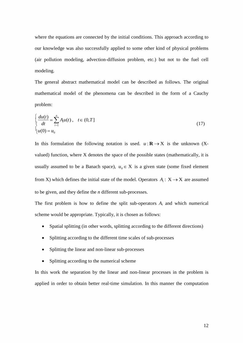
The general abstract mathematical model can be described as follows. The original

mathematical model of the phenomena can be described in the form of a Cauchy

problem:

0

1

)0(

],0(,)()(

uu

TttuAdt

tdu n

i

i (17)

In this formulation the following notation is used. X: Ru is the unknown (X-

valued) function, where X denotes the space of the possible states (mathematically, it is

usually assumed to be a Banach space), X0 u is a given state (some fixed element

from X) which defines the initial state of the model. Operators iA : XX are assumed

to be given, and they define the n different sub-processes.

The first problem is how to define the split sub-operators Ai and which numerical

scheme would be appropriate. Typically, it is chosen as follows:

Spatial splitting (in other words, splitting according to the different directions)

Splitting according to the different time scales of sub-processes

Splitting the linear and non-linear sub-processes

Splitting according to the numerical scheme

In this work the separation by the linear and non-linear processes in the problem is

applied in order to obtain better real-time simulation. In this manner the computation

13

can be solved in parallel, and several sub-problems can be solved analytically. The

effect of the nonlinearity is also studied by using different approximations.

It can be shown [9] that the continuous mathematical model of the porous electrode Eqs.

(4)-(8), (under the assumptions that the coefficients are constant) can be transformed

into the form

)()0,(

],0(,)1,0(,)(

0

2

2

2

xuxu

Ttxufx

u

t

u

(18)

where ),( txuu , is the overpotential between the two phases, 2 is the dimensionless

exchange current density, )(uf is an arbitrary source function, defined by one of the

formulas (10) (11) and (12). For this function the following so called non-negativity

property holds: for any nonnegative scalar s the value of the function at this point )(sf

is also nonnegative, i.e., the implication

0)(0),( uftxu (19)

holds. For this problem the boundary conditions are formulated as follows:

.)()()(),1(

,)()(),0(

12

1

eff

eff

eff

eff

tgRT

FLtItgt

x

u

RT

FLtItgt

x

u

(20)

Here )(1 tg and )(2 tg are the dimensionless currents in the solid phase and the solution

phase, respectively. Two different sub-processes can be defined by using the following

operators:

)(2

1 ufuA is the source operator (21)

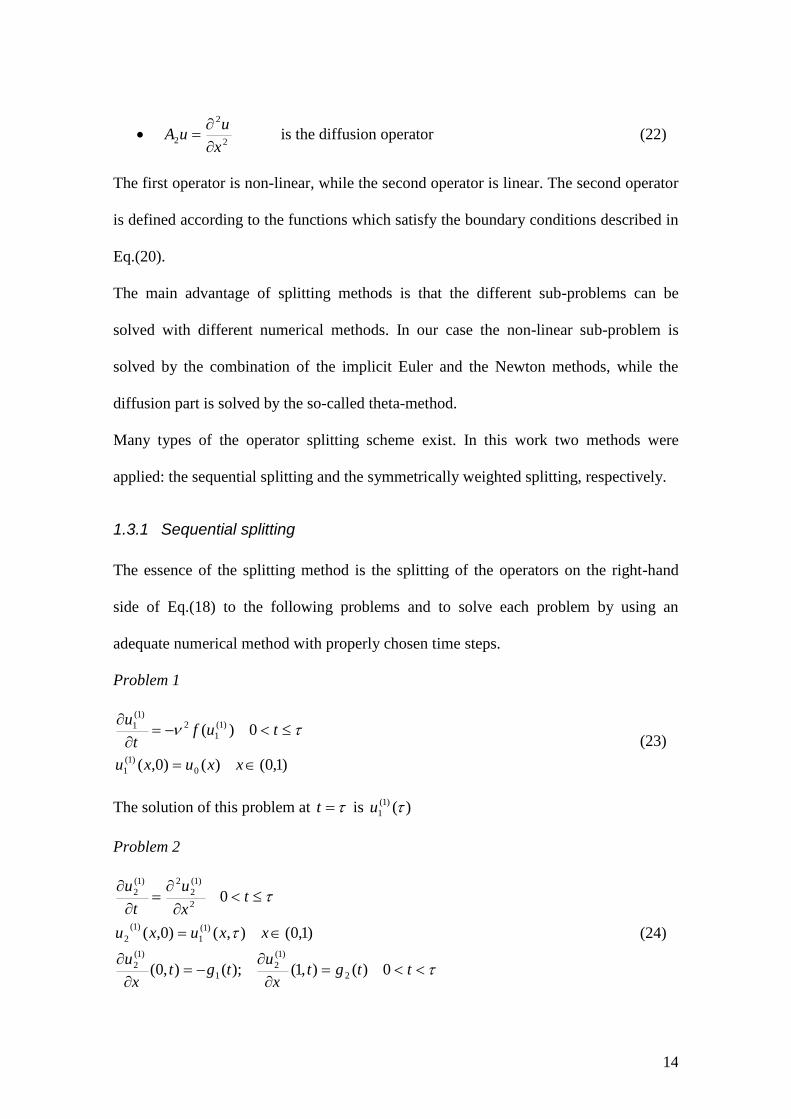
14

2

2

2x

uuA

is the diffusion operator (22)

The first operator is non-linear, while the second operator is linear. The second operator

is defined according to the functions which satisfy the boundary conditions described in

Eq.(20).

The main advantage of splitting methods is that the different sub-problems can be

solved with different numerical methods. In our case the non-linear sub-problem is

solved by the combination of the implicit Euler and the Newton methods, while the

diffusion part is solved by the so-called theta-method.

Many types of the operator splitting scheme exist. In this work two methods were

applied: the sequential splitting and the symmetrically weighted splitting, respectively.

1.3.1 Sequential splitting

The essence of the splitting method is the splitting of the operators on the right-hand

side of Eq.(18) to the following problems and to solve each problem by using an

adequate numerical method with properly chosen time steps.

Problem 1

)1,0()()0,(

0)(

0

)1(

1

)1(

1

2)1(

1

xxuxu

tuft

u

(23)

The solution of this problem at t is )()1(

1 u

Problem 2

ttgtx

utgt

x

u

xxuxu

tx

u

t

u

0)(),1();(),0(

)1,0(),()0,(

0

2

)1(

21

)1(

2

)1(

1

)1(

2

2

)1(

2

2)1(

2

(24)

15

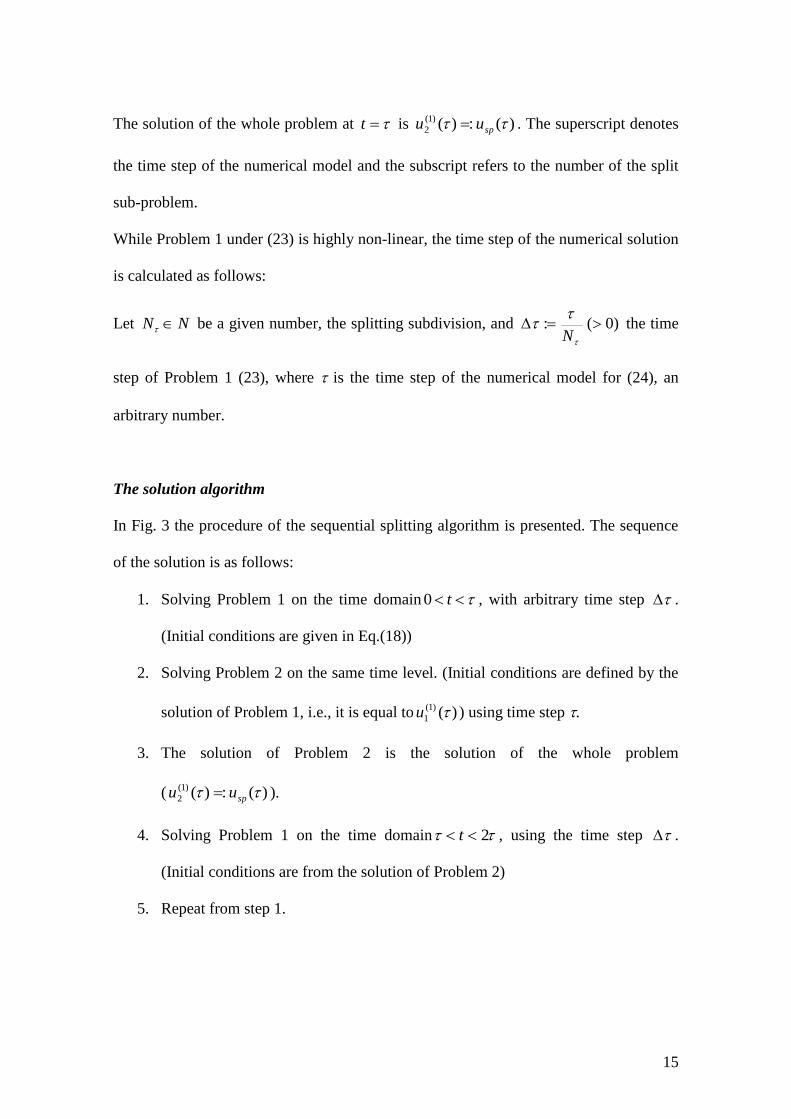
The solution of the whole problem at t is )(:)()1(

2 spuu . The superscript denotes

the time step of the numerical model and the subscript refers to the number of the split

sub-problem.

While Problem 1 under (23) is highly non-linear, the time step of the numerical solution

is calculated as follows:

Let NN be a given number, the splitting subdivision, and )0(:

N the time

step of Problem 1 (23), where is the time step of the numerical model for (24), an

arbitrary number.

The solution algorithm

In Fig. 3 the procedure of the sequential splitting algorithm is presented. The sequence

of the solution is as follows:

1. Solving Problem 1 on the time domain t0 , with arbitrary time step .

(Initial conditions are given in Eq.(18))

2. Solving Problem 2 on the same time level. (Initial conditions are defined by the

solution of Problem 1, i.e., it is equal to )()1(

1 u ) using time step .

3. The solution of Problem 2 is the solution of the whole problem

( )(:)()1(

2 spuu ).

4. Solving Problem 1 on the time domain 2 t , using the time step .

(Initial conditions are from the solution of Problem 2)

5. Repeat from step 1.

16

Figure 3. The sequential splitting method

1.3.2 Symmetrically weighted splitting

The sequential splitting method is not symmetrical with respect to the order of the

operators therefore its accuracy is not high. (We consider this question later.) This

means that using different orderings of the operators typically we obtain different

numerical results. We can symmetrize it, and this approach improves the efficiency of

the algorithm. The idea of the symmetrically weighted method is the following: the

sequentially split solutions are defined in both orderings, and then their average value is

taken for calculating the solution.

In Fig. 4 the process of the symmetrically weighted splitting method is illustrated. The

algorithm of the solution is the following:

1. Solving Problem 1 on the time domain t0 , using arbitrary time step .

(Initial conditions are given)

2. Solving Problem 2 on the same time domain. (Initial conditions are from the

solution of Problem 1)

3. Solving Problem 2‟ (This problem is equivalent to problem 2) on the same time

domain. (Initial conditions are given)

17

4. Solving Problem 1‟ (This problem is equivalent to problem 1) on the same time

domain, using arbitrary time step . (Initial conditions are from the solution of

Problem 2‟)

5. The average of Problem 2 and Problem 1‟ is the solution of the whole problem.

6. Repeat from step 1.

Figure 4. The symmetrically weighted splitting method

1.3.3 The accuracy of the splitting

The exact solution and the split solution of the given problem are denoted by )(tu and

by )(tusp , respectively. By definition, their difference at the point t (at the first

splitting time step) is called local splitting error, which can be written by using the

Landau symbol as

)(O)(u)(u)(Err 1p

spsp

(25)

where p>0 some given number. Then the splitting method is called p-th order splitting.

The splitting is called consistent when Eq.(25) holds uniformly starting for any starting

point t. It is known that, for well-posed problems, when the scheme is consistent and

stable, then it is convergent, too. Most of the numerical schemes applied are convergent,

18

however, the order of decay (of Errsp) is different, which means that the time required to

reach the same accuracy is different. If the order is higher, the method is more precise,

but the computational time might be longer. The trade-off between the precision and the

computational time (practically the cost) is the main optimization problem in real-time

applications.

In appendix 1. we show that the sequential splitting has first order, while the

symmetrically weighted splitting has second order accuracy.

We decrease until the results of two successive numerical experiments differ less than

a given error bound. For a given tau, , i.e., N is chosen such that increasing the

value of N does not change the numerical result significantly [22].

1.3.4 Benefits and drawbacks

The benefits of the splitting methods are the following:

1) Easier theoretical investigation. In order to show the convergence, we should

prove the consistency and stability. It is almost evident that when the sub-

problems are consistent then the total method is also consistent. For the stability

we can use the result that if both sub-problems are contractive then this implies

the stability. Of the whole method. We note that to show these properties for the

split sub-problems is easier task due to the simpler structure of the split sub-

problems.

2) Choice of suitable numerical method. We can apply different numerical methods

to the different sub-problems with different step-sizes. In our approach the time-

steps for the linear and non-linear split subproblems were quite different and

with this approach we could significantly increase the efficiency of the global

algorithm.

19

3) Applicability of the existing software products. The sub-problems are standard

therefore we can use the existing program packages to their solution (like

diffusion part, chemistry, etc.)

4) Use of numerical-analytical methods. If one of the sub-problems can be solved

analytically then there is no need to apply numerical method to its solving. This

may increase the efficiency of the method.

5) Preservation of main qualitative properties. When in the split sub-problems the

required qualitative properties (like non-negativity preservation, maximum

principle, etc.) are preserved then the complete numerical algorithm also has

this property.

However the splitting methods have some drawbacks as well:

1) Local splitting error. New source of the error appears and it disappears only

under some (mostly unrealistic) conditions. However our approach makes

possible its handling.

2) Handling of the boundary conditions. The problem is how it is possible to

describe the boundary conditions for the different sub-problems of different

type? ( E.g. for the diffusion and advection parts.)

2 Experimental

2.1 General approach to compare the numerical results

The exact solution was calculated by applying the implicit Euler method (IEM) with a

very short time step (10-6

s). The relative error of the numerical schemes was calculated

by using the following equation:

pr

pr

y

yyErr

(26)

20

where pry is the exact solution, and y is the solution compared. The positive sign of

the relative error means that the solution is lower than the exact one, and if it is

negative, then the solution is higher than the exact one.

In Table 4 the parameters of the numerical models are listed. Column „Symbol‟ (e.g.

EE.1, EE.2) are the short codes of the model‟s numerical parameter set, which will be

used further on. ‟Type‟ shows the numerical scheme used: Implicit Euler (in this case

no splitting method was used), sequential splitting and symmetrically weighted

splitting. The time step ( ) is the time length between two solution sequences, and the

splitting subdivision is the number of the sub-division of the problem (23) ( N ). The

other parameters as the applied current density, the current sweep rate and the kinetics

are always mentioned in the figure‟s caption, separately.

Table 4. The parameters of the numerical models

Symbol Type Time step / s Splitting subdiv.

EE.1 Implicit Euler 0.001 -

EE.2 Implicit Euler 0.0001 -

EE.3 Implicit Euler 0.00001 -

SQ.1.1 Sequential splitting 0.001 1

SQ.1.10 Sequential splitting 0.001 10

SQ.2.1 Sequential splitting 0.0001 1

SQ.2.10 Sequential splitting 0.0001 10

SQ.3.1 Sequential splitting 0.00001 1

SQ.3.10 Sequential splitting 0.00001 10

SY.1.1 Symmetrically weighted s. 0.001 1

SY.1.10 Symmetrically weighted s. 0.001 10

SY.2.1 Symmetrically weighted s. 0.0001 1

SY.2.10 Symmetrically weighted s. 0.0001 10

SY.3.1 Symmetrically weighted s. 0.00001 1

SY.3.10 Symmetrically weighted s. 0.00001 10

3 Results and discussion

The elucidation of the effect of the kinetics on the error of the scheme is very

problematic using complex equations, such as Eq.(15). Therefore, only linear and

21

Butler-Volmer kinetics will be studied. In these cases the effects of the non-linearity on

the scheme accuracy can be determined. The simulation result of the complex diffusion

limitation kinetics will be compared with the measurements calculating the V-I and

series of the current step curves of the system.

3.1 The effect of constant current

3.1.1 Linear kinetics

In Fig. 5 the accuracy of the sequential splitting method and the symmetrically weighted

method were analyzed at different time steps, by using linear kinetics and applying

constant current. As it was expected, the smaller the time step, the smaller the relative

error. The sharp peaks (around 0.25s) in Fig. 5 are artifacts due to the computation of

the relative error, and not to the numerical method. It is a consequence of the fact, that

the inaccuracy becomes very high when the denominator in Eq.(26) approaches zero.

a)

b)

Figure 5. The error of the sequential splitting (a) and the symmetrically weighted splitting (b)

method. Liner kinetics at different time steps, applying constant current (0.1A)

22

3.1.2 Butler-Volmer kinetics

The results obtained when the IEM with different time steps and Butler-Volmer kinetics

are applied and those of the exact solution were compared in Fig. 6. It is plausible that

the relative error diminishes when the time step decreases. After applying the current a

positive and a negative peak appear, because the approximation error depends on the

time-derivative of the rapidly changing solution at the transient state. After the complete

charging of the double layer the relative error becomes practically zero in all cases. This

means that the steady-state in the physical system is reached.

However, the accuracy is sufficient mainly at constant current simulation, because in the

case of alternating current or current sweeps transient effect dominates at short times,

i.e., when the derivative is changing very fast. This can lead to a higher relative error of

the IEM in comparison with the splitting methods.

Figure 6. The relative error of the IEM method incorporating Butler-Volmer kinetics, at different

time steps and applying constant current (0.1A)

Fig. 7 shows the relative error when Butler-Volmer kinetics was considered, and the

sequential and the symmetrically weighted methods were used at different time steps

and different splitting sub-divisions. The relative error did not converge to zero when

the splitting technique was used, however, it was stabilized at a constant, relatively low

23

value. Furthermore, this constant value is decreasing if the time step is decreased or the

sub-division is increased. Owing to its minor value, the error can be neglected, however

it has some mathematical interest regarding to the solution of a combination of linear

and non-linear operators. When Problems 1 and 2 are solved in one step (i.e., by IEM)

the slight instability of the non-linear operator is compensated by the diffusion operator.

But if the operators are solved separately (i.e., by splitting), this error correction ability

is slightly lower than in the joint solution steps.

a)

b)

Figure 7. The relative error of the sequential splitting (a) and the symmetrically weighted splitting

(b) method incorporating Butler-Volmer kinetics, at different time steps and applying constant

current (0.1A)

The symmetrically weighted splitting method (Fig. 7 b) is more accurate than the

sequential one, but increasing the subdivision does not necessarily decreases the relative

error. The symmetrically weighted solution is the average of the differently ordered

sequential split solutions. When the non-linear part is the first step of the calculation,

the diffusion-like operator has a smoothing effect, which can “repair” the non-linear

subproblem error. But when the diffusion operator is solved first, the non-linear

operator can spoil the accuracy.

24

It is worth emphasizing that under linear kinetics when both operators are linear and

stable in themselves, the relative error approaches to zero and does not become a

constant value as in the case of the Butler-Volmer (non-linear) kinetics. This effect is

caused by the non-linearity of the source operator, which will be analyzed in Fig. 10.

3.2 The investigation of current sweeps

In Fig. 8 the error functions of the sequential splitting method and the symmetrically

weighted method obtained at different time steps, by using Butler-Volmer kinetics and

0.1 As-1

current sweep rate are displayed. In the sequential splitting cases the relative

error decreases with the decrease of the time step and with the increase of the splitting

subdivision, respectively. The relative error of models SQ.2, SQ.3 is less than 5 percent.

a)

b)

Figure 8. The error of sequential splitting (a) and symmetrically weighted splitting (b) methods at

different time steps, Butler-Volmer kinetics, rate of current sweep was 0.1As-1

.

The relative error of the symmetrical splitting method, as it is expected, is smaller than

that of the sequential method, however, the courses of the curves are different. An

increase of the number of the splitting subdivision does not necessarily causes the

25

decrease of the relative error. However, the solution with bigger subdivision (smaller

) can be more accurate and the error of the longest time step has a surprisingly very

good accuracy, because of the parabolic type curve. It can be interpreted in terms of the

change of the linearity of the source operator. At low currents the operator is practically

linear since the exponential function can be linearized at low perturbations. At higher

currents the operator becomes non-linear and simultaneously the model is switched

from the stable to the unstable state.

Fig. 9 shows the error of the implicit Euler method (IEM) under different time steps by

using Butler-Volmer kinetics and applying current sweeps 0.1 As-1

and 1 As-1

. At low

sweep rates and long time steps the model became unstable after 0.5 seconds (at 0.05 A)

and the relative error grew above 100%. However, the accuracy in the case of the short

time steps is very good. At higher sweep rates the accuracy and stability of the IEM

gradually become worse. Even at short time steps the error starts to increase (Fig. 9 b),

while the system is still stable, however, the stability also deteriorates with time. Longer

time steps together with high sweep rate conditions cannot be applied because of a fast

loss of accuracy and stability. This means that many situations occurring in real-time

applications cannot be treated by this method. Even at shorter time steps the

preservation of qualitative properties, namely the non-negativity of the derivate cannot

be guaranteed as seen at small perturbations of the EE.2 run on Fig. 9.

On the other hand, by using any of the splitting methods, even at long time steps, the

model remains stable, and the absolute value of the relative error is less than 20%. In the

case of the symmetrical method the relative error does not exceed 2%.

26

Table 5. Comparison of the used numerical methods(constant current was applied [1A])

Method Running Time / s Err / ‰

EE.3 301065 0.001110

SQ.3.10 224563 0.002343

SY.3.10 151517 0.002345

EE.1 4561 -6.507659

SQ.1.10 4618 0.123172

SY.1.10 3088 0.0123256

On Table 5. the used numerical methods are compared in running time and numerical

accuracy. The results show the use of splitting methods shorten the computational time,

in the same time preserving the accuracy of the method. Therefore the splitting methods

enhance the applicability of the numerical model effectively even at high sweep rates.

a)

b)

Figure 9. The error of IEM at different time steps, Butler-Volmer kinetics. Current sweeps are a)

0.1 As-1

and b) 1 As-1

.

3.3 The spatial potential distribution

The effect of the non-linearity on the spatial distribution of the local overpotential is

demonstrated in Fig. 10. The difference between the exact and the splitting solutions,

which was observed in the time domain (Fig. 9), also appears. The symmetrical splitting

evidently gives more accurate solution than the sequential method. The decrease of time

27

step results in a more accurate solution even at higher currents (Fig. 10). The relative

error, however, starts to increase when the derivative of the local overpotential reaches a

critical value at a given time step. In Fig. 10 b the results obtained at a higher current

density are shown. Despite the non-uniform potential distribution at shorter time step,

more accurate solution is obtained. The splitting method leads to approximately exact

solution, when the spatial derivative is small.

a)

b)

Figure 10. Spatial distribution of the local overpotential at constant current densities (a) 0.1 Acm-2

and (b) 0.5 A cm-2

by using different numerical schemes

3.4 The preservation of qualitative properties

The preservation of qualitative properties is as important as the relative error

(convergence) of the scheme. In the following two qualitative properties will be

examined: the non-negativity of the derivative and the asymptotic solution [4,5], , i.e.,

doubling of the Tafel slope.

The solution of a numerical scheme can be very accurate in absolute value, even if it

converges alternately to the exact solution. The alternating nature of the numerical

28

solution, however, can lead to failure in real-time controlling. The splitting methods

avoid the alternation of the derivative, which allows their use in real-time simulation.

The doubling of the Tafel slope [6] is demonstrated in Fig. 11 when the V-I curves were

obtained under different time steps and at a current sweep rate of 1 As-1

. The Tafel

slopes are practically the same as calculated from the precise solution both in the lower

and the higher polarization regimes, even if the accuracy is very bad at SY.1.10. The

IEM method under high sweep rate and the same numerical conditions was unstable

(Fig. 9b), and it stopped before the end of the simulation even if the shortest time step

was applied. Furthermore, the accuracy exceeded 10% before the IEM model lost its

stability. The symmetrical splitting method expands the stability of the calculation with

an increase of the relative error, however, it is less than 10%.

a)

b)

Figure 11. The relative error (a) and the calculated V-I curves (b) at different time steps by using

symmetrically weighted splitting and Butler-Volmer kinetics. The current sweep rate is 1 As-1

.

3.5 The comparison of the simulated and measured data

Two of the kinetic parameter sets were simulated and the results were compared with

the measured data. The measured V-I curves and the simulated ones are presented in

29

Fig. 12. The measured data were obtained on the same MEA after the application of two

different pretreatments. One of the set of data () was measured after the intense use of

the membrane, the second set of data () was measured after holding at OCV for an

hour. A high activation loss can be observed at the beginning when the MEA was

conditioned at open-circuit. However, after reaching 0.3 Acm-2

this activation loss

diminishes, and its behavior approaches to that of the intensively used MEA. The

simulation of the V-I curves (continuous lines 1-3) was based on the calculated

parameters in

30

Table 3. Curve 1 was calculated by using = 1 and n = 1 (Tafel slope = -60 mV/dec

and i0= 7.2210-8

Acm-2

) without any further parameter optimization. Curve 2 was

calculated by using = 0.5 and n = 1 (Tafel slope = -110 mV / dec) and i0 = 7.2210-5

Acm-2

. In this case the fit is seemingly rather poor. The difference in the small current

region is not negligible, however, at higher currents when the ohmic loss prevails or the

mass transport is the rate-determining step, the difference is smaller. The variation of

the exchange current density and the apparent transfer coefficient in the low and the

higher current regimes have been reported in [8,20], and it was assigned to the change

in the reaction path. The curve 3 was calculated by using = 0.5 and n = 1 (Tafel slope

= -110 mV / dec) varying only the value of the exchange current density. The optimum

value of the exchange current density was chosen as i0 = 7.2210-6

Acm-2

. This curve

fits well at the low current densities, however, below 0.5 V, possibly due to the change

of the kinetics, the fitting becomes poor. The change of the kinetics is related to the

reduction of the oxides that covered the Pt surface [19].

31

Figure 12. The measured and the simulated V-I curves of an Air / H2 fuel cell at 80oC and ambient

pressure, E-TEK Gas Diffusion Electrodes with Pt loading of 0.5 mg cm-2

for both the anode and

the cathode

The application of splitting techniques provides the opportunity to simulate transients in

“normal” time window on a PC, because this technique is only slightly sensitive to rapid

changes. For the simulation of series of current steps the same parameters were used as

for curve 1 in Fig. 12. Fig. 13 shows the measured and the simulated results,

respectively. In the lower potential ranges the cell was under load, while in the upper

potential ranges the electrode relaxed. The shape of the curves is very similar but the

potential maxima in the relaxation ranges of the simulated curves are definitely lower

than the measured values even if the simulated V-I curve fits the measured data fairly

well. In our simulation the maximum rate of diffusion was approximated by the

respecting limiting current, which means that the diffusional relaxation has been

neglected. But if the variation of the oxygen concentration had been taken into account,

the potential relaxation would have been even slower, and the simulation curves would

have been below the current simulated curve. Consequently, the deviation between the

measured and the simulated curves shown in Fig. 13 cannot be interpreted by the

neglected oxygen diffusion.

In our previous work [21] the effect of the current stepping on the Tafel slope was

demonstrated. During these experiments the potential periodically varied between 0.45

V and 0.75 V and a decrease of the Tafel slope was observed. The latter effect was

related to the formation of oxides on the electrode surface. When the potential of the

fuel cell alternates rapidly and with a high amplitude, the surface coverage might

substantially influence the behavior of a functioning fuel cell. This effect has not been

taken account in the simulation and requires further investigation.

32

215 216 217 218 219

0,6

0,7

0,8

0,9

1,015

Ce

ll V

olta

ge

/ V

time / s

Figure 13. Measured ( ■ ) and simulated (continuous line) transients of an Air / H2 fuel cell. The

current was stepped between 0 and 0.4 Acm-2

with 1 Hz and 50 % duty ratio.

4 Conclusions

The real-time simulation of fuel cells has become an important task regarding the

control and automation of functioning applications. The operator splitting methods

provides an opportunity to monitor the actual state of fuel cells in real time, because it

splits the complex system to different subsystems, and the most effective numerical

methods can be applied for every subsystem. While the general approach of the

symmetrical and the sequential splitting method was described in other papers [16, 17,

18], the application for fuel cells, where one operator is linear and one is non linear, is

novel.The computation can be executed simultaneously, which is a great advantage in

the case of the usage of multi-core processors or FPGAs (field-programmable gate

array). In this work the splitting of the linear and non-linear subsystems was applied for

the fuel cell model developed. The accuracy and the preservation of the qualitative

properties of the model were examined by using linear and non-linear (Butler-Volmer)

33

kinetics. The splitting method was more accurate than the mostly used implicit Euler

method (IEM) when the case of linear kinetics and constant current was simulated.

When exponential kinetics was considered the relative error of the splitting methods

was less than 0.2%, which that of the IEM was 0.02%. In the case of the splitting

method, this deviation did not diminish with time as it happened by using the IEM

method, but decreased when the time step was decreased or the splitting subdivision

was increased. The increase of the splitting subdivision yielded substantially more

accurate result, when the first ordered (sequential) splitting scheme was applied, but the

second order (symmetrical) scheme was more accurate in every respect. The

symmetrical splitting method was found more useful for the simulation of high current

sweeps rates, because it was stable at two magnitude longer time steps and the total

accuracy was better than that of the IEM.

The complex limiting current kinetics was compared with the measurements. The

parameters of the cell were calculated by the composition of the catalyst layer and no

further parameter optimization was done. A good fit was found for the simulation of V-I

curves, but the simulated and the measured relaxation states showed a substantial

difference in the case of the examination of current steps. These results indicate that the

effect of variation of the surface coverage (e.g., oxides, chemisorbed species) during

fast changes of potential or current, which occur many times in real applications, can

also be treated.

Acknowledgement

34

Financial support of the National Office of Research and Technology (OMFB-

00356/2007 and OMFB-00121-00123/2008) and National Scientific Research Fund

(OTKA K71771)(G.I.)) are acknowledged.

References

[1] J. Kim, S-M. Lee, S. Srinivasan, J. Electrochem. Soc, 142 (1995) 2670.

[2] S, Srinivasan, Fuel Cells From Fundamental to Applications, Springer, New York, 2006.

[3] P. M. Gomadam, J. W. Weidner, T. A. Zawodinski, A. P. Saab, J. Electrochem Soc., 150 (2003)

E371.

[4] A.A. Kulikovsky, Electrochem. Comm. 4 (2002) 318.

[5] F. Jaounen, G. Lindbergh, G. Sundholm, J. Electrochem. Soc., 149 (2002) A437.

[6] J. Ihonen, F. Jaouen, G. Lindbergh, A. Lundblad, G. Sundholm, J. Electrochem. Soc., 149 (2002)

A448.

[7] T. Navessin, S. Holdcroft, Q. Wang, D. Song, Z. Liu, M. Eikerling, J. Horsfall, K. V. Lovell, J.

Electroanal. Chem., 567 (2004) 111.

[8] C. Ziegler, H.M. Yu, O.J. Schumacher, J. Electrochem. Soc., 152 (2005) A1555.

[9] Faragó, I., Inzelt, G., Kornyik, M., Kriston, Á., Szabó, T., Stabilization of a numerical model through

the boundary conditions for the real-time simulation of fuel cells. International Conference on Systems,

Computing Sciences and Software Engineering. (2007)

[10] V.R. Subramaniam, V. Boovargavan, V.D. Diwakar, Electrochem. and Solid-State Lett., 10 (2007)

A255.

[11] W. Hundsdorfer, J. Verwer: Numerical Solution of Time-Dependent Advection-Diffusion-Reaction

Equations. Springer, 2003.

[12] S. Litster, N. Djilali, Electrochim. Acta, 52 (2007) 3849.

[13] A.A. Kulikovsky, Electrochem. Comm, 4 (2002) 845.

[14] A. Z. Weber, J. Newman, J. Electrochem. Soc., 151 (2004) A311.

[15] J, Newman, K. E. Thomas-Alyea: Electrochemical systems, John Wiley & Sons, New Jersey, 2004.

pp. 517[16] Z. Zlatev and I. Dimov: "Computational and Numerical Challenges in Environmental

Modelling". Elsevier, Amsterdam-Boston-Heidelberg-London-New York-Oxford-Paris-San Diego-San

Francisco-Singapore-Sydney-Tokyo, 2006.

[17] J. Bartholy, I. Faragó, Á. Havasi, Splitting method and its application in air pollution modelling,

Időjárás, Quart. J. HMS, 105 (2001) 39-58.

[18] P. Csomós, I. Faragó, Á. Havasi , Weighted sequential splittings and their analysis, Comput. Math.

Appl., 50 (2005) 1017-1031.

[19] A. Damjanovic, V. Brusic, Electrochim. Acta, 12 (1967) 615.

[20] A. Parthasarathy, C. R. Martin, S. Srinivasan, J. Electrochem. Soc., 138 (1991) 916.

[21] Á. Kriston, G. Inzelt, J. Appl. Electrochem., 38, 415 (2008)

[22] P. Csomós, I. Faragó, Error analysis of the numerical solution of split differential equations,

Mathematical and Computer Modelling, 48 (2008) 1090-1106.

35

List of figures:

Figure 1. Schematic drawing of the membrane electrode assembly (MEA)

Figure 2. Comparison of different kinetics Figure 3. The sequential splitting method Figure 4. The symmetrically weighted splitting method Figure 5. The error of the sequential splitting (a) and the symmetrically weighted

splitting (b) method. Liner kinetics at different time steps, applying constant current

(0.1A) Figure 6. The relative error of the IEM method incorporating Butler-Volmer kinetics, at

different time steps and applying constant current (0.1A)

Figure 7. The relative error of the sequential splitting (a) and the symmetrically

weighted splitting (b) method incorporating Butler-Volmer kinetics, at different time

steps and applying constant current (0.1A) Figure 8. The error of sequential splitting (a) and symmetrically weighted splitting (b)

methods at different time steps, Butler-Volmer kinetics, rate of current sweep was

0.1As-1

. Figure 9. The error of IEM at different time steps, Butler-Volmer kinetics. Current

sweeps are a) 0.1 As-1

and b) 1 As-1

. Figure 10. Spatial distribution of the local overpotential at constant current densities (a)

0.1 Acm-2

and (b) 0.5 A cm-2

by using different numerical schemes Figure 11. The relative error (a) and the calculated V-I curves (b) at different time steps

by using symmetrically weighted splitting and Butler-Volmer kinetics. The current

sweep rate is 1 As-1

.

Figure 12. The measured and the simulated V-I curves of an Air / H2 fuel cell at 80oC

and ambient pressure, E-TEK Gas Diffusion Electrodes with Pt loading of 0.5 mg cm-2

for both the anode and the cathode