Simulation of Supersonic Combustion Using Variable Prandtl ...

Abstract

KEISLTER, PATRICK G. Simulation of Supersonic Combustion Using Variable

Turbulent Prandtl/Schmidt Numbers Formulation. (Under the direction of Dr. Hassan A.

Hassan.)

A turbulence model that allows for the calculation of the variable turbulent

Prandtl (Prt) and Schmidt (Sct) numbers as part of the solution is presented. The model

also accounts for the interactions between turbulence and chemistry by modeling the

corresponding terms. Four equations are added to the baseline k-ζ turbulence model: two

equations for enthalpy variance and its dissipation rate to calculate the turbulent

diffusivity, and two equations for the concentrations variance and its dissipation rate to

calculate the turbulent diffusion coefficient. The variable Prt/Sct turbulence model is

used to simulate the SCHOLAR supersonic combustion experiments. The experiments

include one model with normal hydrogen injection into a vitiated airstream at Mach 2.0,

while the other injects hydrogen at Mach 2.5 and an angle of 30° to the vitiated airstream.

Two sets of calculations are presented for each experiment, one where the turbulent

Prandtl and Schmidt numbers are constant and one where they are allowed to vary. Two

chemical kinetic models are employed for each calculation: a seven species/seven

reaction model where the reaction rates are temperature dependent and a nine

species/nineteen reaction model where the reaction rates are dependent on both pressure

and temperature.

The simulation of the vectored injection experiment predicts an earlier ignition

than what is suggested by the experimental data. Also, the downstream pressure is

underpredicted. The temperature distribution in the downstream portion of the combustor

is higher with the variable Prt/Sct model than with the constant model, which places it

within the experimental scatter. When the computed temperature profiles are subjected

to the same curve fit as the experimental scatter, very good agreement is observed. The

simulation of the normal injection experiment showed similar results, with

underprediction of downstream pressures and less overall combustion. However, the

variable Prt/Sct model does show improved results over the constant model. The variable

model shows a complex shock-boundary layer interaction that extends upstream of the

backward facing step. The pressure distribution along the bottom wall is very closely

matched in this region, but downstream, the pressures are still underpredicted. A

pressure “plateau” effect that is seen in the experimental data suggests that an area of

large separation or intense combustion exists in the region immediately below the

hydrogen injector. This is not reproduced in any of the simulations. In general the two

chemical kinetic mechanisms provide nearly identical results. Finally, it is shown that

the computed results are highly dependent on the compressibility correction for the

turbulence model. When this term is neglected, unstart conditions result for both the

vectored injection experiment and the normal injection experiment.

Simulation of Supersonic Combustion Using Variable

Turbulent Prandtl / Schmidt Numbers Formulation

by

Patrick Keistler

A thesis submitted to the Graduate Faculty of

North Carolina State University

in partial fulfillment of the

requirements for the Degree of

Master of Science

Mechanical and Aerospace Engineering

Raleigh, North Carolina

2006

Approved by:

___________________________ ___________________________

Jack R. Edwards D. Scott McRae

___________________________

Hassan A. Hassan

Chair of Advisory Committee

ii

Biography

Patrick Garrett Keistler was born in Concord, North Carolina on May 1st, 1982.

One of the major influences on his educational choices was his participation in the Air

Force Junior ROTC at Central Cabarrus High School. During this time his interest in

aviation was sparked. With this and an interest in physics and mathematics, the obvious

choice was to study aerospace engineering at North Carolina State University. It was not

until his senior year that an interest in computational fluid dynamics developed, but that

was enough time to decide that it was what he wanted to pursue. Patrick plans to

continue his education in the pursuit of a Ph.D. at NC State.

iii

Acknowledgements

There are a number of people I would like to thank for their support through the

course of this work. First is my thesis advisor Dr. Hassan A. Hassan, who has taught me

many valuable lessons, and provided excellent guidance. Another individual who has

been an invaluable source of information and assistance is Dr. Xudong Xiao. I would not

be to this point without his expertise and knowledge. Also, I would like to thank my

parents, Max and Kristy Keistler for their continued motivation and support throughout

my college career. The interest they show in my work is very encouraging. Finally, I

would like to thank Mr. George Rumford, the program manager of the Defense Test

Resource Management Center’s Test and Evaluation/Science and Technology program

for funding this effort under the Hypersonic Test focus area.

iv

Table of Contents

List of Figures .................................................................................................................... vi

List of Tables ................................................................................................................... viii

List of Symbols .................................................................................................................. ix

1 Introduction................................................................................................................. 1

2 Governing Equations .................................................................................................. 5

2.1 Reacting Gas Equation Set.................................................................................. 5

2.1.1 Navier-Stokes Equations............................................................................. 5

2.1.2 Thermodynamic Relations .......................................................................... 7

2.2 Governing Equations in Vector Form................................................................. 8

2.3 Reynolds and Favre Averaging........................................................................... 9

2.4 Chemical Kinetics............................................................................................. 11

2.4.1 Jachimowski Chemical Mechanism.......................................................... 13

2.4.2 Connaire et al. Chemical Mechanism ....................................................... 13

2.5 Turbulence Closure........................................................................................... 15

2.5.1 k-ζ Model .................................................................................................. 16

2.5.2 Variable Turbulent Prandtl Number Model.............................................. 19

2.5.3 Variable Turbulent Schmidt Number Model ............................................ 22

2.5.4 Turbulence / Chemistry Interactions......................................................... 25

2.6 Complete Equation Set ..................................................................................... 26

2.6.1 Solution Methods...................................................................................... 26

3 Experimental Overview ............................................................................................ 27

3.1 The SCHOLAR Experiments ........................................................................... 27

3.1.1 Vectored Injection Case............................................................................ 28

3.1.2 Normal Injection Case .............................................................................. 30

3.2 CARS Measurement Techniques...................................................................... 32

3.3 Experimental Data Fitting................................................................................. 33

4 Implementation ......................................................................................................... 35

4.1 Multiblock Parallel Approach........................................................................... 35

v

4.2 Computational Geometry.................................................................................. 35

4.3 Wall and Inlet Boundary Conditions ................................................................ 39

4.3.1 Wall Boundaries........................................................................................ 39

4.3.2 Inflow and Outflow Boundaries................................................................ 41

5 Results and Discussion ............................................................................................. 42

5.1 General Results ................................................................................................. 42

5.2 Vectored Injection Model ................................................................................. 47

5.2.1 Variable Prt / Sct Runs .............................................................................. 47

5.2.2 Constant Prt / Sct Runs.............................................................................. 56

5.3 Normal Injection Model.................................................................................... 60

5.3.1 Constant Prt / Sct Run ............................................................................... 61

5.3.2 Variable Prt / Sct Run................................................................................ 64

6 Conclusions............................................................................................................... 71

References......................................................................................................................... 73

Appendix A: Governing Equations Vectors ..................................................................... 78

Appendix B: Transformation to Generalized Coordinates ............................................... 80

Appendix C: Chemical Kinetic Mechanism Parameters .................................................. 84

Appendix D: Complete Equation Set in Vector Form...................................................... 88

Appendix E: Numerical Formulation................................................................................ 92

vi

List of Figures

Figure 3.1: Schematic of Vectored Injection SCHOLAR Experiment............................. 28

Figure 3.2: Detail of Vectored Hydrogen Injector............................................................ 29

Figure 3.3: Schematic of Normal Injection SCHOLAR Experiment ............................... 30

Figure 3.4: Detail of Normal Hydrogen Injector .............................................................. 31

Figure 3.5: Example of CARS Measurements and Curve Fit (Plane 6, y = 18.2 mm)..... 34

Figure 4.1: Block Layout and H2 Injector Detail for Vectored Injection ......................... 36

Figure 4.2: Vectored Block Layout with CARS Survey Planes Highlighted ................... 37

Figure 4.3: Block Layout and H2 Injector Detail for Normal Injection............................ 38

Figure 5.1: Pitot Pressure Profile at Vitiated Air Nozzle Exit.......................................... 44

Figure 5.2: Temperature Slice with Adiabatic Wall Temperature.................................... 45

Figure 5.3: Wall Temperature vs. Run Time at Three Locations (Ref [11]) .................... 46

Figure 5.4: Temperature Slice of Plane 6 at y = 18.2 mm (Connaire).............................. 48

Figure 5.5: Mole Fraction Slices of Plane 6 at y = 18.2 mm (Connaire).......................... 49

Figure 5.6: 5th Degree Polynomial Fits of Exp. and Computed Temperature (Run 1) ..... 50

Figure 5.7: 5th Degree Polynomial Fits of Exp. and Computed Mole Fractions (Run 1) . 50

Figure 5.8: Experimental Surface Fits of Temperature for Vectored Case ...................... 51

Figure 5.9: Temperature Contours for Run 1.................................................................... 52

Figure 5.10: Nitrogen and Oxygen Mole Fractions for Run 1.......................................... 52

Figure 5.11: Temperature from Runs 1 and 2 (Left: Jach., Right: Connaire)................... 53

Figure 5.12: Wall Pressures for Runs 1 and 2 .................................................................. 54

Figure 5.13: OH Mole Fractions for Runs 1 and 2 (Left: Connaire, Right: Jach.) ........... 55

Figure 5.14: Turbulent Prantl Number (left) and Turbulent Schmidt Number (right) ..... 56

Figure 5.15: Temperature Contours for Run 3.................................................................. 57

Figure 5.16: Nitrogen and Oxygen Mole Fractions for Run 3......................................... 58

Figure 5.17: Temperature from Runs 3 and 4 (Left: Jach., Right: Connaire)................... 59

Figure 5.18: Wall Pressures for Runs 3 and 4 .................................................................. 60

Figure 5.19: Temperature Contours for Run 5.................................................................. 61

vii

Figure 5.20: Mole Fraction Contours for Run 5 (left: N2, right: O2) ................................ 62

Figure 5.21: Bottom Wall Pressure for Run 5 .................................................................. 63

Figure 5.22: Temperature Contours for Run 6.................................................................. 64

Figure 5.23: Mach Contours on Symmetry Plane for Run 6 ............................................ 65

Figure 5.24: Mach Contours on Symmetry Plane for Run 5 ............................................ 66

Figure 5.25: Mole Fraction Contours for Run 6 (left: N2, right: O2) ................................ 67

Figure 5.26: Bottom Wall Pressure for Runs 5 and 6 ....................................................... 67

Figure 5.27: 3D Hydrogen Mole Fraction Contours for Run 6 ........................................ 68

Figure 5.28: Stream Traces Originating in Hydrogen Injector ......................................... 69

Figure 5.29: Mach Number Contours on Symmetry Plane for Unstart Conditions.......... 70

viii

List of Tables

Table 2.1: Troe Parameters for Connaire et al. Mechanism ............................................. 15

Table 2.2: k-ζ Model Closure Coefficients ....................................................................... 19

Table 2.3: Variable Prandtl Number Model Constants..................................................... 22

Table 2.4: Variable Schmidt Number Model Constants................................................... 25

Table 3.1: Inflow Conditions for Vectored Injection........................................................ 30

Table 3.2: Inflow Conditions for Normal Injection .......................................................... 32

Table 5.1: Runs Presented................................................................................................. 47

Table C.1: Abridged Jachimowski Mechanism Reactions ............................................... 84

Table C.2: Abridged Jachimowski Mechanism Parameters ............................................. 84

Table C.3: Connaire et al. Mechanism Reactions............................................................. 85

Table C.4: Connaire et al. Mechanism Parameters........................................................... 86

Table C.5: Connaire et al. Mechanism Third Body Efficiencies ...................................... 87

ix

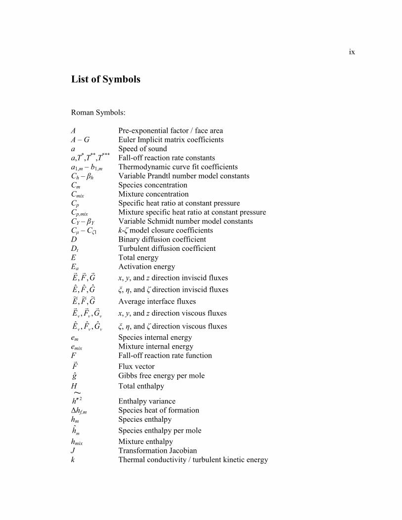
List of Symbols

Roman Symbols:

A Pre-exponential factor / face area

A – G Euler Implicit matrix coefficients

a Speed of sound

a,T*,T**,T*** Fall-off reaction rate constants

a1,m – b1,m Thermodynamic curve fit coefficients

Ch – βh Variable Prandtl number model constants

Cm Species concentration

Cmix Mixture concentration

Cp Specific heat ratio at constant pressure

Cp,mix Mixture specific heat ratio at constant pressure

CY – βY Variable Schmidt number model constants

Cµ – Cζ1 k-ζ model closure coefficients

D Binary diffusion coefficient

Dt Turbulent diffusion coefficient

E Total energy

Ea Activation energy

GFErrr,, x, y, and z direction inviscid fluxes

GFE ˆ,ˆ,ˆ ξ, η, and ζ direction inviscid fluxes

GFE~,~,~

Average interface fluxes

vvv GFErrr,, x, y, and z direction viscous fluxes

vvv GFE ˆ,ˆ,ˆ ξ, η, and ζ direction viscous fluxes

em Species internal energy

emix Mixture internal energy

F Fall-off reaction rate function

Fr Flux vector

g Gibbs free energy per mole

H Total enthalpy ~2h ′′ Enthalpy variance

∆hf,m Species heat of formation

hm Species enthalpy

mh Species enthalpy per mole

hmix Mixture enthalpy

J Transformation Jacobian

k Thermal conductivity / turbulent kinetic energy

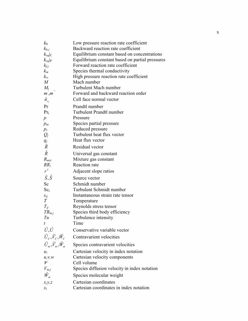
x

k0 Low pressure reaction rate coefficient

kb,i Backward reaction rate coefficient

keq|C Equilibrium constant based on concentrations

keq|P Equilibrium constant based on partial pressures

kf,i Forward reaction rate coefficient

km Species thermal conductivity

k∞ High pressure reaction rate coefficient

M Mach number

Mt Turbulent Mach number

m’,m

” Forward and backward reaction order

ixn Cell face normal vector

Pr Prandtl number

Prt Turbulent Prandtl number

p Pressure

pm Species partial pressure

pr Reduced pressure

Qj Turbulent heat flux vector

qj Heat flux vector

Rr Residual vector

R Universal gas constant

Rmix Mixture gas constant

RRi Reaction rate ±r Adjacent slope ratios

SS ˆ,r

Source vector

Sc Schmidt number

Sct Turbulent Schmidt number

sij Instantaneous strain rate tensor

T Temperature

Tij Reynolds stress tensor

TBm,j Species third body efficiency

Tu Turbulence intensity

t Time

UU ˆ,r

Conservative variable vector

CCC WVU~,

~,

~ Contravarient velocities

mmm WVU~,

~,

~ Species contravarient velocities

ui Cartesian velocity in index notation

u,v,w Cartesian velocity components

V Cell volume

Vm,j Species diffusion velocity in index notation

mW Species molecular weight

x,y,z Cartesian coordinates

xi Cartesian coordinates in index notation

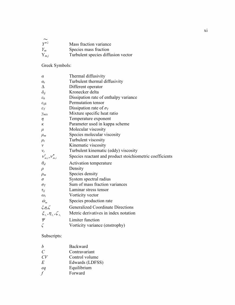
xi

~2Y ′′ Mass fraction variance

Ym Species mass fraction

Ym,j Turbulent species diffusion vector

Greek Symbols:

α Thermal diffusivity

αt Turbulent thermal diffusivity

∆ Different operator

δij Kronecker delta

εh Dissipation rate of enthalpy variance

εijk Permutation tensor

εY Dissipation rate of σY γmix Mixture specific heat ratio

η Temperature exponent

κ Parameter used in kappa scheme

µ Molecular viscosity

µm Species molecular viscosity

µt Turbulent viscosity

ν Kinematic viscosity

νt Turbulent kinematic (eddy) viscosity

imim ,, ,νν ′′′ Species reactant and product stoichiometric coefficients

θd Activation temperature

ρ Density

ρm Species density

σ System spectral radius

σY Sum of mass fraction variances

τij Laminar stress tensor

ωi Vorticity vector

mω& Species production rate

ξ,η,ζ Generalized Coordinate Directions

iii xxx ζηξ ,, Metric derivatives in index notation

Ψ Limiter function

ζ Vorticity variance (enstrophy)

Subscripts:

b Backward

C Contravariant

CV Control volume

E Edwards (LDFSS)

eq Equilibrium

f Forward

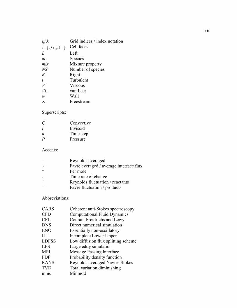
xii

i,j,k Grid indices / index notation

21

21

21 ,, +++ kji Cell faces

L Left m Species

mix Mixture property

NS Number of species

R Right

t Turbulent

V Viscous

VL van Leer

w Wall

∞ Freestream

Superscripts:

C Convective

I Inviscid

n Time step

P Pressure

Accents:

– Reynolds averaged

~ Favre averaged / average interface flux

^ Per mole

. Time rate of change

‘ Reynolds fluctuation / reactants

“ Favre fluctuation / products

Abbreviations:

CARS Coherent anti-Stokes spectroscopy

CFD Computational Fluid Dynamics

CFL Courant Freidrichs and Lewy

DNS Direct numerical simulation

ENO Essentially non-oscillatory

ILU Incomplete Lower Upper

LDFSS Low diffusion flux splitting scheme

LES Large eddy simulation

MPI Message Passing Interface

PDF Probability density function

RANS Reynolds averaged Navier-Stokes

TVD Total variation diminishing

mmd Minmod

xiii

Other symbols:

∂ Partial derivative

∇ Gradient operator

1 Introduction

There has always been a need for air-breathing aerospace vehicles to travel higher

and faster. Whether it is for more affordable access to orbit, or for defense applications,

the need for engines that are capable of propelling an aircraft to hypersonic speeds is

clear. Traditional turbojets, in the extreme case, can operate from zero velocity up to

around Mach 3. At this point the compressor starts to do more harm than good. By

removing the compressor, and thus the need for a turbine, a ramjet engine is created.

Ramjets can operate in the range from Mach 3 or 4 to about Mach 5 [19]. At Mach 5,

decelerating the flow to subsonic speeds for combustion becomes unreasonable due to the

excessive temperatures and thus dissociation of fuel rather than combustion. This

illustrates the need for a supersonic combustion ramjet, also known as a scramjet. Rather

than mixing and combusting fuel at subsonic speeds, the incoming air is allowed to

remain supersonic. The task of mixing and combusting supersonically is a daunting one

and the simulation of this process can be equally as difficult. Important factors in the

simulation of these types of flows include, but are not limited to, the specification of the

turbulent Prandtl and Schmidt numbers and the consideration of turbulence/chemistry

interactions. The turbulent Prandtl and Schmidt numbers are inherently variable in the

complex three-dimensional flows that are characteristic of current proposed scramjet

designs. Since classic turbulence models assume these numbers to be constant and

specified ahead of time, a new turbulence model that allows these numbers to vary and

also accounts for turbulence/chemistry interactions is required [16][43]. One such model

is utilized herein. Another factor that has received little attention in the literature is the

role of compressibility on high speed mixing and combustion. It is well known that

mixing-layer growth rate decreases with increasing Mach number [40]. This

phenomenon becomes especially important in supersonic combustion devices due to the

fact that compressibility effects reduce the ability of the fuel to mix with air at supersonic

speeds, resulting in less overall combustion.

2

Some efforts have been made to move toward the calculation, rather than

specification, of the turbulent Prandtl and Schmidt numbers as part of the solution.

Methods based on the mixing length have been employed as early as 1975, by Reynolds,

to calculate both the turbulent Prandtl and Schmidt numbers [30]. In 1988, Nagano

developed a two equation model for calculating the turbulent diffusivity, which was used

in conjunction with the k-ε turbulence model [28]. However, the model was not

developed for high speed flow and thus does not include the effects of compressibility.

This model provided the framework for most of the work to follow. In 1993, Sommer et

al. developed a variable turbulent Prandtl number model using methods very similar to

those used by Nagano [35]. This model was also derived from the incompressible energy

equation rather than the compressible energy equation, so compressibility effects, which

have been determined to be quite important, are not accounted for. Two additional

equations were added to the base incompressible k-ε turbulence model, temperature

variance, and its dissipation rate. Solving these four equations allowed for the calculation

of the turbulent diffusivity. In general the results for high Mach number, low wall

temperature cases were improved over those utilizing the k-ε model alone. In 1999,

another approach was taken by Guo et al. to create a variable turbulent Schmidt number

model [18]. In addition to the k-ε turbulence model, Guo modeled the turbulent species

diffusion vector with a single transport equation. A genetic algorithm technique was

applied to efficiently obtain the model constants. Again, the results were improved over

the baseline k-ε model for a jet-in-crossflow application.

A company known as Combustion Research and Flow Technology, Inc. (CRAFT

Tech) have been investigating the use of variable turbulent Prandtl number methodology

for propulsive type flows since 2000 [25]. The formulation is based largely on the work

of Sommer and Nagano, but they did also investigate algebraic stress models in addition

to the k-ε model. Again the model equations for temperature variation and its dissipation

rate are based on the low speed energy equation. The pressure gradient term and the term

responsible for energy dissipation are ignored. The current work does not make these

simplifications since such assumptions are not valid for scramjet type flows. The model

3

was later applied by CRAFT Tech to a Large Eddy Simulation (LES) of reacting and

non-reacting shear layers at high speeds [6][7]. The purpose of this work was to generate

data to be used in improving RANS models. Compressibility corrections were applied in

this work, but the model constants were modified in an ad hoc manner, without

significant validation. The model was extended to include variable Prt and variable Sct in

2005 [4].

In 2005, Xiao et al. presented two similar approaches, one for calculating the

turbulent Prandtl number (Prt) as part of the solution [42] and one for calculating the

turbulent Schmidt number (Sct) as part of the solution [41]. Each of these new models

used the k-ζ turbulence model of Robinson and Hassan as a base [31]. With the addition

of two equations each, enthalpy variance and its dissipation rate for the variable Prt model

and concentrations variance and its dissipation rate for the variable Sct model, the

turbulent diffusivity and the turbulent diffusion coefficient were able to be determined.

Improvements were observed for a coaxial jet flow [9] with the variable Sct model, and

improvements in heat flux predictions were seen with the variable Prt model. The

variable Sct model was later applied to the supersonic combustion experiment of Burrows

and Kurkov [5], while using a probability density function (PDF) to address the

turbulence/chemistry interactions. In general the variable Sct formulation worked well

for both mixing and reacting supersonic flows; however, the PDF method for addressing

turbulence/chemistry interactions did not necessarily improve the results [22]. A

complete turbulence model, where both the Prt and Sct are calculated as part of the

solution was presented by Xiao et al. in 2006 [43]. This work, which employed a new

modeling approach for the turbulence/chemistry interactions, showed improvement in

predictions for both the coaxial jet and the Burrows and Kurkov combustor. The work

also reinforced the fact that the turbulence/chemistry interactions must be accounted for.

The latest work, which most of the content herein is based on, applied the complete

model to the SCHOLAR supersonic combustion experiments [24][23]. These results are

discussed in Chapter 5.

4

The SCHOLAR combustor has been simulated extensively by Rodriguez and

Cutler in conjunction with the actual experiments. Initially, only mixing was considered

[13], then the reacting case [10]. Rodriguez and Cutler later continued the work in a

more comprehensive study [33]. The simulation utilized the VULCAN CFD code,

developed at NASA Langley Research Center. The k-ω turbulence model was used with

various constant values of Prt and Sct. The computed results were seen to vary greatly

with the specification of these parameters. The best results were obtained with Prt = 0.9

and Sct = 1.0, therefore, the constant Prt/Sct runs in the current work use these values.

The computational grid used in the current work was also developed from a grid

originally generated by Rodriguez.

5

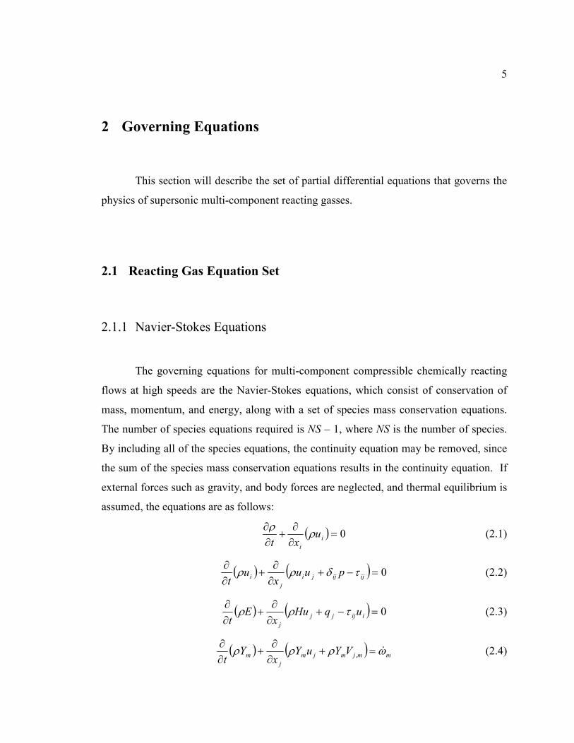
2 Governing Equations

This section will describe the set of partial differential equations that governs the

physics of supersonic multi-component reacting gasses.

2.1 Reacting Gas Equation Set

2.1.1 Navier-Stokes Equations

The governing equations for multi-component compressible chemically reacting

flows at high speeds are the Navier-Stokes equations, which consist of conservation of

mass, momentum, and energy, along with a set of species mass conservation equations.

The number of species equations required is NS – 1, where NS is the number of species.

By including all of the species equations, the continuity equation may be removed, since

the sum of the species mass conservation equations results in the continuity equation. If

external forces such as gravity, and body forces are neglected, and thermal equilibrium is

assumed, the equations are as follows:

( ) 0=∂∂

+∂∂

i

i

uxt

ρρ

(2.1)

( ) ( ) 0=−+∂∂

+∂∂

ijijji

j

i puux

ut

τδρρ (2.2)

( ) ( ) 0=−+∂∂

+∂∂

iijjj

j

uqHux

Et

τρρ (2.3)

( ) ( ) mmjmjm

j

m VYuYx

Yt

ωρρρ &=+∂∂

+∂∂

, (2.4)

6

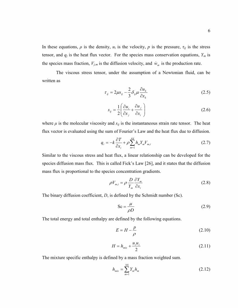
In these equations, ρ is the density, ui is the velocity, p is the pressure, τij is the stress

tensor, and qj is the heat flux vector. For the species mass conservation equations, Ym is

the species mass fraction, Vj,m is the diffusion velocity, and mw& is the production rate.

The viscous stress tensor, under the assumption of a Newtonian fluid, can be

written as

k

k

ijijijx

us

∂

∂−= µδµτ3

22 (2.5)

∂

∂+

∂

∂=

i

j

j

iij

x

u

x

us

2

1 (2.6)

where µ is the molecular viscosity and sij is the instantaneous strain rate tensor. The heat

flux vector is evaluated using the sum of Fourier’s Law and the heat flux due to diffusion.

∑=

+∂∂

−=NS

m

immm

i

i VYhx

Tkq

1

,ρ (2.7)

Similar to the viscous stress and heat flux, a linear relationship can be developed for the

species diffusion mass flux. This is called Fick’s Law [26], and it states that the diffusion

mass flux is proportional to the species concentration gradients.

i

m

m

imx

Y

Y

DV

∂∂

= ρρ , (2.8)

The binary diffusion coefficient, D, is defined by the Schmidt number (Sc).

Dρµ

=Sc (2.9)

The total energy and total enthalpy are defined by the following equations.

ρp

HE −= (2.10)

2

iimix

uuhH += (2.11)

The mixture specific enthalpy is defined by a mass fraction weighted sum.

∑=

=NS

m

mmmix hYh1

(2.12)

7

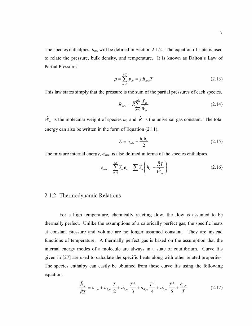
The species enthalpies, hm, will be defined in Section 2.1.2. The equation of state is used

to relate the pressure, bulk density, and temperature. It is known as Dalton’s Law of

Partial Pressures.

TRpp mix

NS

m

m ρ== ∑=1

(2.13)

This law states simply that the pressure is the sum of the partial pressures of each species.

∑=

=NS

m m

m

mixW

YRR

1ˆ

ˆ (2.14)

mW is the molecular weight of species m, and R is the universal gas constant. The total

energy can also be written in the form of Equation (2.11).

2

iimix

uueE += (2.15)

The mixture internal energy, emix, is also defined in terms of the species enthalpies.

∑∑

−==

= m

mm

NS

m

mmmixW

TRhYeYe

ˆ

ˆ

1

(2.16)

2.1.2 Thermodynamic Relations

For a high temperature, chemically reacting flow, the flow is assumed to be

thermally perfect. Unlike the assumptions of a calorically perfect gas, the specific heats

at constant pressure and volume are no longer assumed constant. They are instead

functions of temperature. A thermally perfect gas is based on the assumption that the

internal energy modes of a molecule are always in a state of equilibrium. Curve fits

given in [27] are used to calculate the specific heats along with other related properties.

The species enthalpy can easily be obtained from these curve fits using the following

equation.

T

bTa

Ta

Ta

Taa

TR

h m

mmmmm

m ,14

,5

3

,4

2

,3,2,15432ˆ

ˆ+++++= (2.17)

8

The species enthalpy in this equation is defined on a per mole basis. To obtain the

enthalpy per unit mass, simply multiply by the species molecular weight. Specific heat,

entropy, and Gibbs free energy can be calculated in a similar manner.

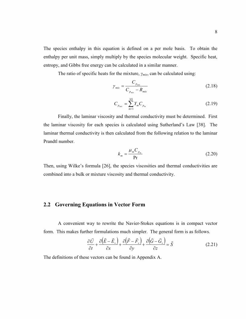
The ratio of specific heats for the mixture, γmix, can be calculated using:

mixp

p

mixRC

C

mix

mix

−=γ (2.18)

∑=

=NS

m

pmp mmixCYC

1

(2.19)

Finally, the laminar viscosity and thermal conductivity must be determined. First

the laminar viscosity for each species is calculated using Sutherland’s Law [38]. The

laminar thermal conductivity is then calculated from the following relation to the laminar

Prandtl number.

Pr

mpm

m

Ck

µ= (2.20)

Then, using Wilke’s formula [26], the species viscosities and thermal conductivities are

combined into a bulk or mixture viscosity and thermal conductivity.

2.2 Governing Equations in Vector Form

A convenient way to rewrite the Navier-Stokes equations is in compact vector

form. This makes further formulations much simpler. The general form is as follows.

( ) ( ) ( )

Sz

GG

y

FF

x

EE

t

U vvvr

rrrrrrr

=∂

−∂+

∂

−∂+

∂

−∂+

∂∂

(2.21)

The definitions of these vectors can be found in Appendix A.

9

2.3 Reynolds and Favre Averaging

While the Navier-Stokes equations describe continuum fluid flow down to the

smallest scales of turbulent motion, the discrete computational grids on which the

equations are solved are unable to resolve such small scales of motion. The small

turbulence scales are very important however, in dissipating energy from larger scale

motion and the mean flow. The traditional approach to this problem is not to resolve the

smallest features of the flow, but rather to model them using the local characteristics and

time history of the flow. This provides a macroscopic view of the affects of turbulence

on the mean flow.

There are certainly alternatives to modeling the turbulence. One such alternative

is direct numerical simulation (DNS), in which the exact Navier-Stokes equations are

resolved down to the smallest turbulence scales. This requires many times more grid

points than a solution where the turbulence is completely modeled, and the requirement is

ever steeper with increasing Reynolds numbers. Another alternative is to resolve some of

the large scale turbulent features and model the scales that occur on the sub-grid level.

This is known as large eddy simulation (LES). This is a compromise, but it still requires

a significantly higher resolution than simulations that model all turbulence scales. Due to

the size of modern engineering problems and the limited computing power that is

available, a completely modeled approach is adopted in the current work.

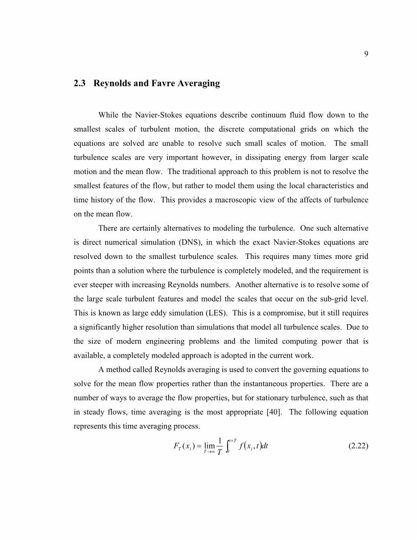
A method called Reynolds averaging is used to convert the governing equations to

solve for the mean flow properties rather than the instantaneous properties. There are a

number of ways to average the flow properties, but for stationary turbulence, such as that

in steady flows, time averaging is the most appropriate [40]. The following equation

represents this time averaging process.

( )∫+

∞→=

Tt

ti

TiT dttxf

TxF ,

1lim)( (2.22)

10

The instantaneous flow property is represented by f(xi,t) while FT(xi) is the time averaged

flow property. The instantaneous flow properties can then be expressed by the time

averaged mean property plus a fluctuation.

qqq ′+= (2.23)

Here, q represents any flow property; q is the time averaged quantity and q′ is the

fluctuation. This averaging is applied to the velocity and pressure fluctuations.

Applying this time averaging technique to the Navier-Stokes equations results in

what is known as the Reynolds Averaged Navier-Stokes (RANS) equations. While this

method works well for incompressible flows, more variables must be taken into account

if the flow is compressible, namely density and temperature. However, if the same

Reynolds averaging technique is used, terms arise that have no analogue to those in the

incompressible equations. To alleviate this problem, a different type of averaging is

introduced, Favre, or mass-weighted averaging. This average is obtained from the

following equation.

( ) ( )∫+

∞→=

Tt

tii

Tdttxqtxq ,,lim

1~ ρρ

(2.24)

Here, q~ represents the Favre averaged quantity, and, just as before, the instantaneous

quantity can be written as:

qqq ′′+= ~ (2.25)

When averaging the equations, correlation terms appear that are not necessarily zero.

Consider the averaging of the product of any two variables.

( )( ) ψϕψϕψϕϕψψϕψϕψψϕϕϕψ ′′+=′′+′+′+=′+′+= (2.26)

The terms with only one fluctuating term become zero when averaged, but the product of

two fluctuating properties is not necessarily zero if there is a correlation between them.

The density, pressure, stress tensor, heat flux, and species production rate are represented

using the Reynolds average, while the other variables use the Favre average.

mmmiii

ijijij

qqq

ppp

ωωω

τττρρρ

′+=′+=

′+=′+=′+=

&&&,

,,, (2.27)

11

TTTHHHEEE

YYYVVVuuu mmmmimimiiii

′′+=′′+=′′+=

′′+=′′+=′′+=~

,~

,~

,~

,~

,~,,,

(2.28)

Substituting these quantities into the Navier-Stokes equations and performing the

prescribed averaging results in the Favre averaged Navier-Stokes equations, still known

as the RANS equations [43].

( ) 0~ =∂∂

+∂∂

i

i

uxt

ρρ

(2.29)

( ) ( ) mjm

j

m

j

mj

j

m uYx

YD

xYu

xY

tωρρρρ &+

′′′′−

∂∂

∂∂

=∂∂

+∂∂

~~~~

(2.30)

( ) ( ) [ ]ijij

ji

ij

j

i uuxx

puu

xu

t′′′′−

∂∂

+∂∂

−=∂∂

+∂∂

ρτρρ ~~~ (2.31)

( ) ( ) ( )[ ] ( )huqx

uuux

uHx

Et

ii

i

ijijj

i

i

i

′′′′+∂∂

−′′′′−∂∂

=∂∂

+∂∂

ρρτρρ ~~~ (2.32)

Three new terms are introduced in this form of the equations, the turbulent stress tensor,

ijuu ′′′′− ρ , the turbulent heat flux vector, hui ′′′′ρ , and the turbulent species diffusion

vector, jmuY ′′′′− ρ . These terms are approximated by the turbulence model to be defined in

Section 2.5. The turbulent stress tensor is also known as the Reynolds stress tensor.

2.4 Chemical Kinetics

Finite rate chemical kinetics is used to track chemical reactions in the present

work. This method is based on the Law of Mass Action (LMA) [26]. This law

determines the rate of change of the concentration of a single species in a multi-

component flow. This rate is then incorporated into the source term for the species

conservation equations.

12

A chemical mechanism consists of a collection of exchange/recombination

reactions and third body reactions, which when combined, result in the global reaction

such as that for hydrogen oxidation. The Law of Mass Action for

exchange/recombination reactions is:

∏∏=

′′

=

′ −=NS

m

mib

NS

m

mifiimim CkCkRR

1

,

1

,,, νν (2.33)

For third body reactions, which require any third molecule to initiate, the equation

becomes:

−= ∑∏∏

==

′′

=

′NS

m

imm

NS

m

mib

NS

m

mifi TBCCkCkRR imim

1

,

1

,

1

,,, νν

(2.34)

Cm is the species concentration, or molar density, which is the species density divided by

the molecular weight. The stoichometric coefficients for the reactants are designated by

ν’ and for the products, ν”. The effects of the third body are combined into a single term

called the third body efficiency, TBm,i. Each species has a third body efficiency for each

third body reaction. The forward reaction rate coefficient, kf,i, is determined by the

Arrhenius Law. It takes the following form.

)/exp( TATk df θη −= (2.35)

The parameters A, η, and θd are specific to the chemical kinetic mechanism and will be

discussed in Sections 2.4.1 and 2.4.2. Rather than require a separate set of parameters for

the backward rate coefficient, kb is calculated using the equilibrium coefficient with the

following relation.

)(

ˆ

101325mm

PeqCeq

b

f

TRkk

k

k′−′′

== (2.36)

The above equation also demonstrates the conversion of the equilibrium constant from a

partial pressure basis to a concentration basis, as indicated by the subscripts. The

equilibrium constant for a particular reaction can be calculated from the change in Gibbs

free energy.

∆−=

TR

gk

Peq ˆ

ˆexp (2.37)

13

∑ ′−′′=∆NS

m

mmm gg ˆ)(ˆ νν (2.38)

The production rate of each species can be determined using the preceding information.

m

NR

i

iimimm WRR ˆ)(1

,,

′−′′= ∑=

ννω& (2.39)

2.4.1 Jachimowski Chemical Mechanism

The abridged chemical kinetic mechanism of Jachimowski is one of two models

used in this work [21]. The mechanism consists of seven species and seven reactions.

The species are N2, O2, H2, H2O, OH, H, and O. The reactions are listed in Table C.1 of

Appendix C. Note that the first two reactions are third body reactions, where M

represents the third body. Thus, each equation requires a third body (TB) efficiency for

each species. The species H2 has TB = 2.5 for both reactions and H2O has TB = 16.0 for

both reactions. All other species have a third body efficiency of 1.0 for both reactions.

The mechanism parameters, such as the pre-exponential factor and activation energies are

listed in Table C.2.

2.4.2 Connaire et al. Chemical Mechanism

The second chemical model is that of Connaire et al. [8]. This model employs

nine species and nineteen reactions. It is slightly more complicated than the Jachimowski

mechanism, not just in the magnitude of species and reactions, but in the complexity of

the rate expressions. The reactions are listed in Table C.3 of Appendix C. The

mechanism parameters and third body efficiencies that are not equal to one are also listed

in Appendix C. Note that some of the reactions have two listings. Reactions 14 and 19

are expressed as the sum of two rate expressions. Reactions 9 and 15 employ a different

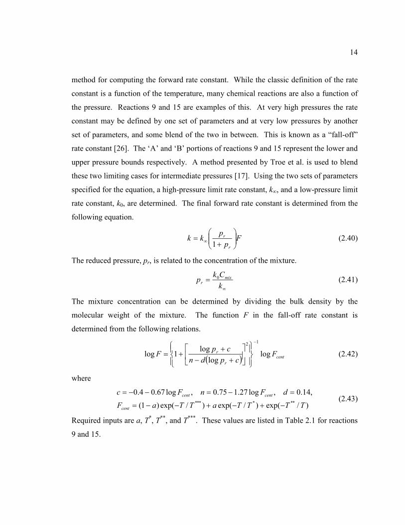
14

method for computing the forward rate constant. While the classic definition of the rate

constant is a function of the temperature, many chemical reactions are also a function of

the pressure. Reactions 9 and 15 are examples of this. At very high pressures the rate

constant may be defined by one set of parameters and at very low pressures by another

set of parameters, and some blend of the two in between. This is known as a “fall-off”

rate constant [26]. The ‘A’ and ‘B’ portions of reactions 9 and 15 represent the lower and

upper pressure bounds respectively. A method presented by Troe et al. is used to blend

these two limiting cases for intermediate pressures [17]. Using the two sets of parameters

specified for the equation, a high-pressure limit rate constant, k∞, and a low-pressure limit

rate constant, k0, are determined. The final forward rate constant is determined from the

following equation.

Fp

pkk

r

r

+= ∞

1 (2.40)

The reduced pressure, pr, is related to the concentration of the mixture.

∞

=k

Ckp mixr

0 (2.41)

The mixture concentration can be determined by dividing the bulk density by the

molecular weight of the mixture. The function F in the fall-off rate constant is

determined from the following relations.

( ) cent

r

r Fcpdn

cpF log

log

log1log

12

−

+−+

+= (2.42)

where

)/exp()/exp()/exp()1(

,14.0,log27.175.0,log67.04.0

****** TTTTaTTaF

dFnFc

cent

centcent

−+−+−−=

=−=−−= (2.43)

Required inputs are a, T*, T

**, and T

***. These values are listed in Table 2.1 for reactions

9 and 15.

15

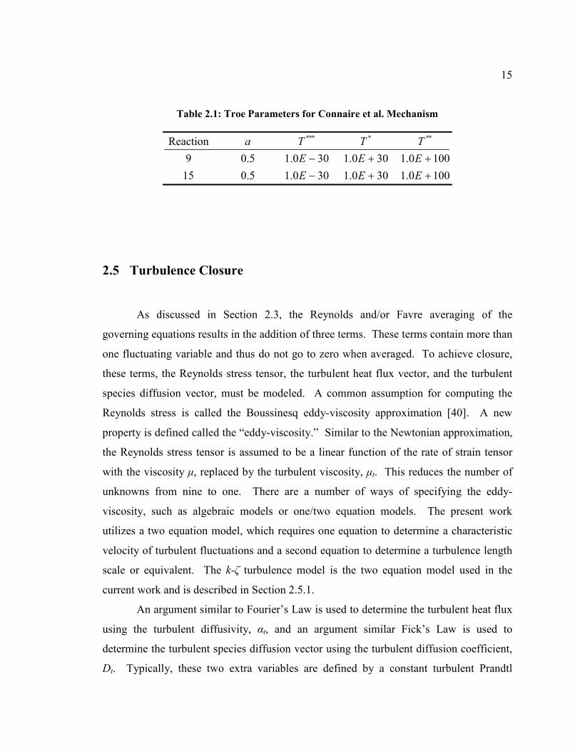
Table 2.1: Troe Parameters for Connaire et al. Mechanism

1000.1300.1300.15.015

1000.1300.1300.15.09

Reaction ******

++−

++−

EEE

EEE

TTTa

2.5 Turbulence Closure

As discussed in Section 2.3, the Reynolds and/or Favre averaging of the

governing equations results in the addition of three terms. These terms contain more than

one fluctuating variable and thus do not go to zero when averaged. To achieve closure,

these terms, the Reynolds stress tensor, the turbulent heat flux vector, and the turbulent

species diffusion vector, must be modeled. A common assumption for computing the

Reynolds stress is called the Boussinesq eddy-viscosity approximation [40]. A new

property is defined called the “eddy-viscosity.” Similar to the Newtonian approximation,

the Reynolds stress tensor is assumed to be a linear function of the rate of strain tensor

with the viscosity µ, replaced by the turbulent viscosity, µt. This reduces the number of

unknowns from nine to one. There are a number of ways of specifying the eddy-

viscosity, such as algebraic models or one/two equation models. The present work

utilizes a two equation model, which requires one equation to determine a characteristic

velocity of turbulent fluctuations and a second equation to determine a turbulence length

scale or equivalent. The k-ζ turbulence model is the two equation model used in the

current work and is described in Section 2.5.1.

An argument similar to Fourier’s Law is used to determine the turbulent heat flux

using the turbulent diffusivity, αt, and an argument similar Fick’s Law is used to

determine the turbulent species diffusion vector using the turbulent diffusion coefficient,

Dt. Typically, these two extra variables are defined by a constant turbulent Prandtl

16

number and turbulent Schmidt number, essentially the same way as their laminar

counterparts. However, in the current work, these two parameters are modeled using two

equations for each that characterize the turbulent heat conduction and turbulent species

diffusion. The formulation of these equations can be found in Sections 2.5.2 and 2.5.3.

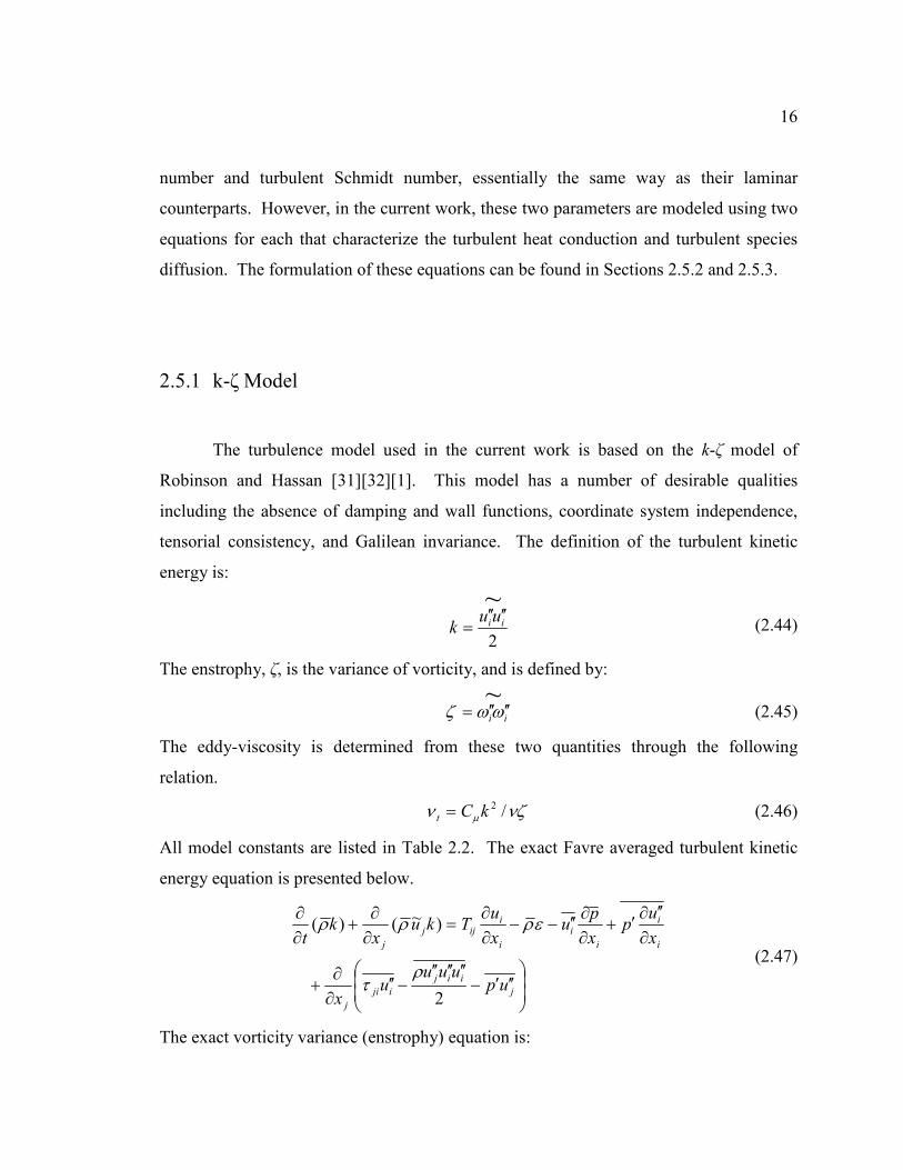
2.5.1 k-ζ Model

The turbulence model used in the current work is based on the k-ζ model of

Robinson and Hassan [31][32][1]. This model has a number of desirable qualities

including the absence of damping and wall functions, coordinate system independence,

tensorial consistency, and Galilean invariance. The definition of the turbulent kinetic

energy is:

2

~iiuuk′′′′

= (2.44)

The enstrophy, ζ, is the variance of vorticity, and is defined by:

~

iiωωζ ′′′′= (2.45)

The eddy-viscosity is determined from these two quantities through the following

relation.

νζν µ /2kCt = (2.46)

All model constants are listed in Table 2.2. The exact Favre averaged turbulent kinetic

energy equation is presented below.

′′′−

′′′′′′−′′

∂∂

+

∂

′′∂′+

∂∂′′−−

∂∂

=∂∂

+∂∂

j

iij

iji

j

i

i

i

i

i

iijj

j

upuuu

ux

x

up

x

pu

x

uTku

xk

t

2

)~()(

ρτ

ερρρ

(2.47)

The exact vorticity variance (enstrophy) equation is:

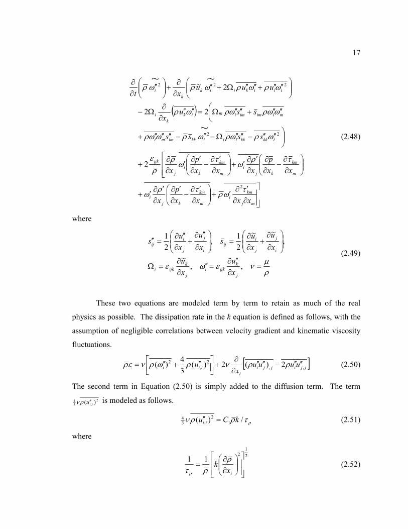
17

( )

∂∂

′∂′+

∂

′∂−

∂

′∂∂

′∂′+

∂∂

−∂∂

∂

′∂′+

∂

′∂−

∂

′∂′∂∂

+

′′′′−′′′′Ω−′′−′′′′′′+

′′′′+′′′′Ω=′′′′∂∂

Ω−

′′′′+′′′′Ω+′′

∂∂

+

′′

∂∂

mj

kmi

m

km

kj

i

m

km

kj

i

m

km

k

i

j

ijk

ikkkkiiikkimmi

miimimimik

k

i

iiikiik

k

i

xxxx

p

x

xx

p

xxx

p

x

ssss

ssux

uuuxt

τωρ

τρω

τρω

τω

ρρ

ε

ωρωρωρωωρ

ωωρωρωρ

ωρωρωρωρ

2

22

222

2

22

2~

~

~~

(2.48)

where

ρµ

νεωε =∂

′′∂=′′

∂∂

=Ω

∂

∂+

∂∂

=

∂

′′∂+

∂

′′∂=′′

,,~

,~~

2

1,

2

1

j

kijki

j

kijki

i

j

j

iij

i

j

j

iij

x

u

x

u

x

u

x

us

x

u

x

us

(2.49)

These two equations are modeled term by term to retain as much of the real

physics as possible. The dissipation rate in the k equation is defined as follows, with the

assumption of negligible correlations between velocity gradient and kinematic viscosity

fluctuations.

[ ]jjijji

i

iii uuuux

u ,,

2

,

2 2)(2)(3

4)( ′′′′−′′′′

∂∂

+

′′+′′= ρρνρωρνερ (2.50)

The second term in Equation (2.50) is simply added to the diffusion term. The term

2

,34 )( iiu ′′ρν is modeled as follows.

ρτρρν /)( 1

2

,34 kCu ii =′′ (2.51)

where

2

12

11

∂∂

=ix

kρ

ρτ ρ

(2.52)

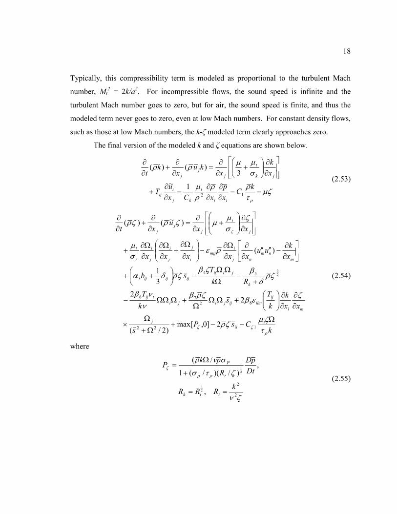
18

Typically, this compressibility term is modeled as proportional to the turbulent Mach

number, Mt2 = 2k/a

2. For incompressible flows, the sound speed is infinite and the

turbulent Mach number goes to zero, but for air, the sound speed is finite, and thus the

modeled term never goes to zero, even at low Mach numbers. For constant density flows,

such as those at low Mach numbers, the k-ζ modeled term clearly approaches zero.

The final version of the modeled k and ζ equations are shown below.

µζτρρ

ρµ

σµµ

ρρ

ρ

−−∂∂

∂∂

−∂∂

+

∂∂

+

∂∂

=∂∂

+∂∂

kC

x

p

xCx

uT

x

k

xku

xk

t

ii

t

kj

iij

jk

t

j

j

j

12

1~

3)~()(

(2.53)

kCsP

s

xx

k

k

Ts

k

T

Rk

Tsb

x

kuu

xxxxx

xxu

xt

tii

j

ml

ij

ilmijjiji

tij

k

jiij

ijijij

m

nm

nj

imij

i

j

j

i

j

i

r

t

j

t

j

j

j

ρζζ

ζ

τζµ

ζρ

ζεβ

ζρβν

νβ

ζρδ

βζβζρδα

ρεσµ

ζσµ

µζρζρ

Ω−−+

Ω+

Ω×

∂∂

∂∂

+ΩΩ

Ω+ΩΩΩ−

+−

Ω

ΩΩ−

++

∂∂

−′′′′∂∂

∂Ω∂

−

∂

Ω∂+

∂Ω∂

∂Ω∂

+

∂∂

+

∂∂

=∂∂

+∂∂

122

82

76

54

3

2]0,max[)2/(

22

3

1

)(

)~()(

2

3

(2.54)

where

ζν

ζτσ

σνρ

ρρ

ζ

2

2

,

,)/)(/(1

/(

2

1

2

1

kRRR

Dt

pD

R

pkP

ttk

t

P

==

+

Ω=

(2.55)

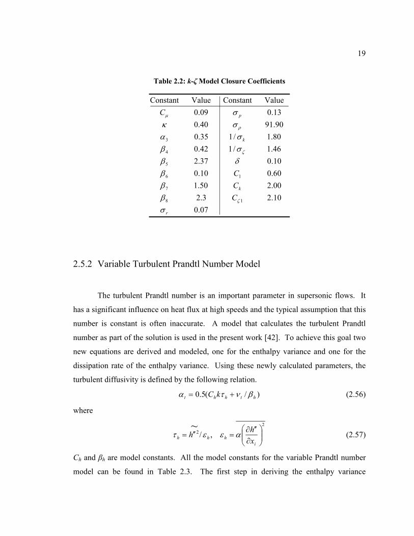
19

Table 2.2: k-ζ Model Closure Coefficients

07.0

10.23.2

00.250.1

60.010.0

10.037.2

46.1/142.0

80.1/135.0

90.9140.0

13.009.0

ValueConstantValueConstant

18

7

16

5

4

3

r

k

k

p

C

C

C

C

σβββ

δβσβσα

σκσ

ζ

ζ

ρ

µ

2.5.2 Variable Turbulent Prandtl Number Model

The turbulent Prandtl number is an important parameter in supersonic flows. It

has a significant influence on heat flux at high speeds and the typical assumption that this

number is constant is often inaccurate. A model that calculates the turbulent Prandtl

number as part of the solution is used in the present work [42]. To achieve this goal two

new equations are derived and modeled, one for the enthalpy variance and one for the

dissipation rate of the enthalpy variance. Using these newly calculated parameters, the

turbulent diffusivity is defined by the following relation.

)/(5.0 hthht kC βντα += (2.56)

where

2

2 ,/~

∂

′′∂=′′=

i

hhhx

hh αεετ (2.57)

Ch and βh are model constants. All the model constants for the variable Prandtl number

model can be found in Table 2.3. The first step in deriving the enthalpy variance

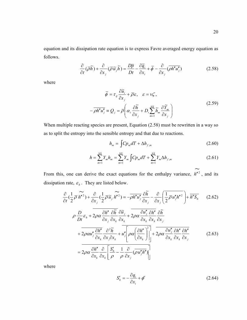
20

equation and its dissipation rate equation is to express Favre averaged energy equation as

follows.

)()~~()

~( j

ji

ij

j

uhxx

q

Dt

pDhu

xh

t′′′′

∂∂

−+∂∂

−=∂∂

+∂∂

ρφρρ (2.58)

where

∂∂

+∂∂

=≡′′′′−

=+∂∂

=

∑=

NS

m j

mmt

j

tjj

j

iij

x

YhD

x

hQuh

x

u

1

~~

~

,,~

αρρ

νζεερτφ

(2.59)

When multiple reacting species are present, Equation (2.58) must be rewritten in a way so

as to split the entropy into the sensible entropy and that due to reactions.

∫ ∆+= mfmm hdTCph , (2.60)

∑∑ ∫∑===

∆+==NS

m

mfm

NS

m

mm

NS

m

mm hYdTCpYhYh1

,

11

(2.61)

From this, one can derive the exact equations for the enthalpy variance, ~2h ′′ , and its

dissipation rate, hε . They are listed below.

hj

jj

jj

j

Shhuxx

huhhu

xh

t′′+

′′′′

∂∂

−∂∂

′′′′−=′′∂∂

+′′∂∂ 222

2

1~

)~

2

1()

2

1(

~~ρρρρ (2.62)

′′′′

∂∂

−′

∂∂

∂

′′∂=

∂

′′∂∂

′′∂∂

′′∂+

∂

′′∂′′+

∂∂∂

∂

′′∂′′+

∂∂

∂

′′∂∂

′′∂+

∂

∂

∂∂

∂

′′∂+

)(1

2

2

~

2

~

2~~

2

22

hux

S

xx

h

x

h

x

h

x

u

x

hu

xx

h

x

hu

x

h

x

h

x

u

x

u

x

h

x

h

Dt

D

j

j

h

kk

jkk

j

k

j

kjk

j

jkk

j

k

j

kj

h

ρρρ

ρα

ραραρα

ραραερ

(2.63)

where

φ ′+∂∂

−=′i

ih

x

qS (2.64)

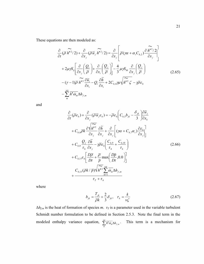
21

These equations are then modeled as:

∑ ∆′′−

−′′+∂∂

−∂∂

′′−−

∂∂

−

∂∂

+

∂∂

+

∂

′′∂+

∂∂

=′′∂∂

+′′∂∂

NS

m

mfm

hh

i

i

i

i

j

j

kk

j

i

i

j

ij

j

ht

j

j

j

hh

hCx

hQ

x

uh

Q

xS

Q

x

Q

xS

x

hC

xhu

xh

t

,

2

4,

2

2

2,

22

~~

~~~

2

~~)1(

3

42

2/)()2/~()2/(

ω

εργζγµργ

ρµγ

ρρµγ

αγαρρρ

&

(2.65)

and

hY

NS

m

mfmh

hh

k

h

h

h

h

jh

j

h

j

hth

jjj

h

k

jjk

jkhhhj

j

h

hhpkC

Dt

pD

pDt

DC

CC

x

hQC

xC

xx

h

x

hkC

x

ubCu

xt

ττ

ωρ

ρρε

ττεργ

τ

εαγαρ

δερερερ

+

∆′′+

++

+−

∂∂

+

∂∂

+∂∂

+∂∂

∂

′′∂+

∂

∂

−−=

∂∂

+∂∂

∑=1

,

2

13,

11,

10,9,

8,

7,

2

6,

5,

~

~

)/(

0.0,max

~

)(

~

~

3)~()(

&

(2.66)

where

νζ

τδρ

k

k

Tb kjk

jk

jk =+= ,3

2 (2.67)

∆hf,m is the heat of formation of species m. τY is a parameter used in the variable turbulent

Schmidt number formulation to be defined in Section 2.5.3. Note the final term in the

modeled enthalpy variance equation, ∑ ∆′′NS

m

mfm hh ,ω& . This term is a mechanism for

22

turbulence/chemistry interactions and the modeling of this term is described in Section

2.5.4.

Table 2.3: Variable Prandtl Number Model Constants

7597.0

5.045.1

0.512.0

86.005.0

55.04.0

25.05.0

87.00648.0

ValueConstantValueConstant

8,

7,

13,6,

12,5,

11,4,

10,2,

9,

h

hh

hh

hh

hh

hh

hh

C

C

CC

CC

CC

CC

CC

β−−

−−

−

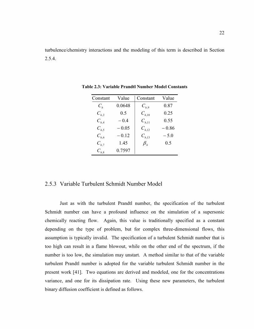
2.5.3 Variable Turbulent Schmidt Number Model

Just as with the turbulent Prandtl number, the specification of the turbulent

Schmidt number can have a profound influence on the simulation of a supersonic

chemically reacting flow. Again, this value is traditionally specified as a constant

depending on the type of problem, but for complex three-dimensional flows, this

assumption is typically invalid. The specification of a turbulent Schmidt number that is

too high can result in a flame blowout, while on the other end of the spectrum, if the

number is too low, the simulation may unstart. A method similar to that of the variable

turbulent Prandtl number is adopted for the variable turbulent Schmidt number in the

present work [41]. Two equations are derived and modeled, one for the concentrations

variance, and one for its dissipation rate. Using these new parameters, the turbulent

binary diffusion coefficient is defined as follows.

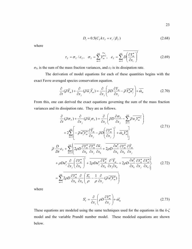
23

)/(5.0 YtYYt kCD βντ += (2.68)

where

∑∑==

∂

′′∂=′′==

NS

m i

mY

NS

m

mYYYYx

YDY

1

2

1

2 ,,/~

εσεστ (2.69)

σY, is the sum of the mass fraction variances, and εY is its dissipation rate.

The derivation of model equations for each of these quantities begins with the

exact Favre averaged species conservation equation.

mjm

j

m

j

mj

j

m uYx

YD

xYu

xY

tωρρρρ &+

′′′′−

∂∂

∂∂

=∂∂

+∂∂

)~~()

~( (2.70)

From this, one can derived the exact equations governing the sum of the mass fraction

variances and its dissipation rate. They are as follows.

∑

∑

=

=

′′+

∂

′′∂−

∂∂

′′′′−+

′′−

∂∂

∂∂

=∂∂

+∂∂

NS

m

mm

j

m

j

mmj

NS

m

mj

j

Y

j

Yj

j

Y

Yx

YD

x

YYu

Yux

Dx

uxt

1

2

1

2

~

2

)~()(

ωρρ

ρσ

ρσρσρ

&

(2.71)

∑

∑

=

=

′′′′

∂∂

−′

∂∂

∂

′′∂=

∂

′′∂∂

′′∂∂

′′∂+

∂∂∂

∂

′′∂′′+

∂

′′∂∂∂′′+

∂∂

∂

′′∂∂

′′∂+

∂

∂

∂

′′∂∂

′′∂+

NS

m

mj

j

Y

kk

m

k

m

j

m

k

j

kj

m

k

mj

k

m

j

j

NS

m j

m

k

m

k

j

k

j

j

m

k

mY

Yux

S

xx

YD

x

Y

x

Y

x

uD

xx

Y

x

YuD

x

Y

xuD

x

Y

x

Y

x

uD

x

u

x

Y

x

YD

Dt

D

1

22

1

)(1

2

2

~

2

~

2~

2

ρρρ

ρ

ρρρ

ρρερ

(2.72)

where

m

j

m

j

Yx

YD

xS ωρ ′+

∂

′′∂∂∂

=′ & (2.73)

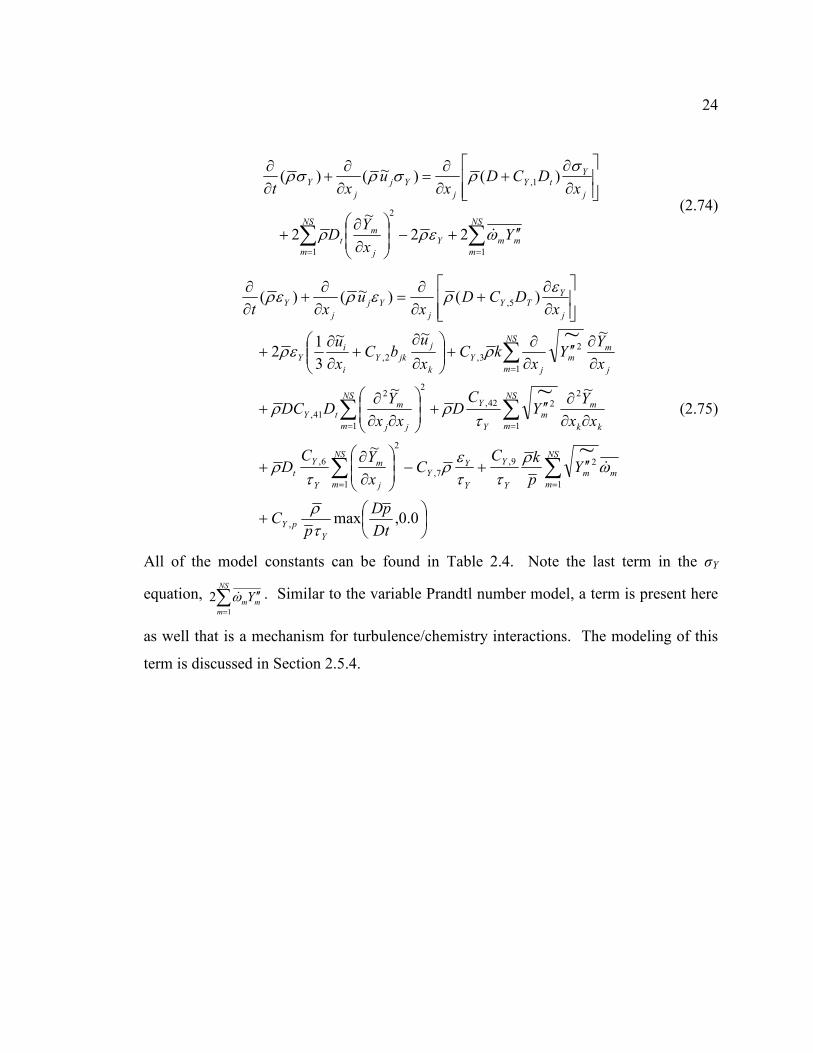
These equations are modeled using the same techniques used for the equations in the k-ζ

model and the variable Prandtl number model. These modeled equations are shown

below.

24

∑ ∑= =

′′+−

∂∂

+

∂∂

+∂∂

=∂∂

+∂∂

NS

m

NS

m

mmY

j

mt

j

YtY

j

Yj

j

Y

Yx

YD

xDCD

xu

xt

1 1

2

1,

22

~

2

)()~()(

ωερρ

σρσρσρ

&

(2.74)

+

′′+−

∂∂

+

∂∂∂

′′+

∂∂∂

+

∂∂

′′∂∂

+

∂

∂+

∂∂

+

∂∂

+∂∂

=∂∂

+∂∂

∑∑

∑ ∑

∑

==

= =

=

0.0,max

~

~~

~~~

3

12

)()~()(

,

1

29,

7,

1

2

6,

1 1

2242,

22

41,

1

2

3,2,

5,

~

~

~

Dt

pD

pC

Yp

kCC

x

YCD

xx

YY

CD

xx

YDDC

x

YY

xkC

x

ubC

x

u

xDCD

xu

xt

Y

pY

NS

m

mm

Y

Y

Y

YY

NS

m j

m

Y

Y

t

NS

m

NS

m kk

mm

Y

Y

jj

mtY

NS

m j

mm

j

Y

k

j

jkY

i

iY

j

YTY

j

Yj

j

Y

τρ

ωρ

ττε

ρτ

ρ

τρρ

ρερ

ερερερ

&

(2.75)

All of the model constants can be found in Table 2.4. Note the last term in the σY

equation, ∑=

′′NS

m

mmY1

2 ω& . Similar to the variable Prandtl number model, a term is present here

as well that is a mechanism for turbulence/chemistry interactions. The modeling of this

term is discussed in Section 2.5.4.

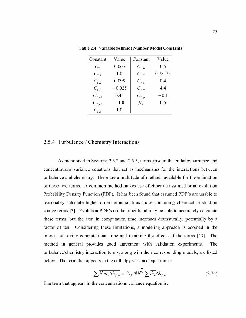
25

Table 2.4: Variable Schmidt Number Model Constants

0.1

5.00.1

1.045.0

4.4025.0

4.0095.0

78125.00.1

5.0065.0

ValueConstantValueConstant

5,

42,

,41,

9,3,

8,2,

7,1,

6,

Y

YY

pYY

YY

YY

YY

YY

C

C

CC

CC

CC

CC

CC

β−

−

−

2.5.4 Turbulence / Chemistry Interactions

As mentioned in Sections 2.5.2 and 2.5.3, terms arise in the enthalpy variance and

concentrations variance equations that act as mechanisms for the interactions between

turbulence and chemistry. There are a multitude of methods available for the estimation

of these two terms. A common method makes use of either an assumed or an evolution

Probability Density Function (PDF). It has been found that assumed PDF’s are unable to

reasonably calculate higher order terms such as those containing chemical production

source terms [3]. Evolution PDF’s on the other hand may be able to accurately calculate

these terms, but the cost in computation time increases dramatically, potentially by a

factor of ten. Considering these limitations, a modeling approach is adopted in the

interest of saving computational time and retaining the effects of the terms [43]. The

method in general provides good agreement with validation experiments. The

turbulence/chemistry interaction terms, along with their corresponding models, are listed

below. The term that appears in the enthalpy variance equation is:

∑∑ ∆′′=∆′′mfmhmfm hhChh ,

2

12,,

~ωω && (2.76)

The term that appears in the concentrations variance equation is:

26

∑∑ ′′=′′mmYmm YCY ωω &&

~2

8,2 (2.77)

For both of these models, mω& is calculated using the mean temperature and mass

fractions. Refer to Table 2.3 and Table 2.4 for the model constants.

2.6 Complete Equation Set

Once the six turbulence equations are incorporated into the reacting gas equation

set, the result is a system of 19 coupled nonlinear partial differential equations. For an

explanation of the solution methods employed, refer to Appendix E. Just as before, the

system of equations can be written in compact vector form for a generalized coordinate

system. See Equation (B.2). Refer to Appendix D for these vectors.

2.6.1 Solution Methods

A finite volume method is used to solve this set of equations. An Essentially

Non-Oscillatory (ENO) and/or Total Variation Diminishing (TVD) scheme is used in

conjunction with the Low Diffusion Flux Splitting Scheme (LDFSS) of Edwards, and the

system is advanced in time using a planar implicit scheme. The viscous and diffusion

terms are evaluated using central differences.

An alternate version of the code was developed, which solved the turbulence

equations separately. The species and conservation equations were solved using the

planar implicit scheme, then the six turbulence equations were solved sequentially using

a three-dimensional scheme. This modification resulted in a significant speed

improvement without changing the computed results.

Appendix E contains a more detailed explanation of the numerical formulation.

27

3 Experimental Overview

This chapter describes the experiments that are used for model validation in the

present study. The experiment is one that has been adopted by a working group of the

NATO Research and Technology Organization for use in CFD validation. The

experiment is known as SCHOLAR. The sections below describe the two experimental

configurations as well as the measurement techniques used.

3.1 The SCHOLAR Experiments

The SCHOLAR experiments were performed at NASA Langley Research

Center’s Direct Connect Supersonic Combustion Test Facility (DCSCTF) [11][29][36].

The experiments were conducted with the intention of being used for CFD validation of

supersonic combustion. The model consists of hydrogen being injected normally or at a

30° angle to a vitiated air stream at Mach 2.0. The initial experiment, with vectored

injection was designed using the VULCAN CFD code [39] with emphasis on avoiding

large regions of subsonic flow. This resulted in a situation where chemical reactions

lagged mixing and combustion did not initiate until far downstream of the injector. This

proved to be difficult for CFD simulations, therefore another experiment, with normal

hydrogen injection was conducted to complement the vectored injection case. Along

with pressure and temperature measurements along the four walls of the combustor, two-

dimensional slices of temperature and species mole fractions were extracted using a

method called coherent anti-Stokes Raman spectroscopy (CARS). These measurements

were taken at a number of planes upstream and downstream of the hydrogen injector.

This technique is described in section 3.2 along with samples of the data obtained.

28

3.1.1 Vectored Injection Case

The first SCHOLAR model employs vectored hydrogen injection [29]. The

hydrogen is injected at Mach 2.5 and a 30° angle to the vitiated air stream. Vitiated air is

the result of hydrogen burning in oxygen enriched air. This technique is used to raise the

enthalpy of the incoming gas to that of hypersonic flight conditions. A schematic of the

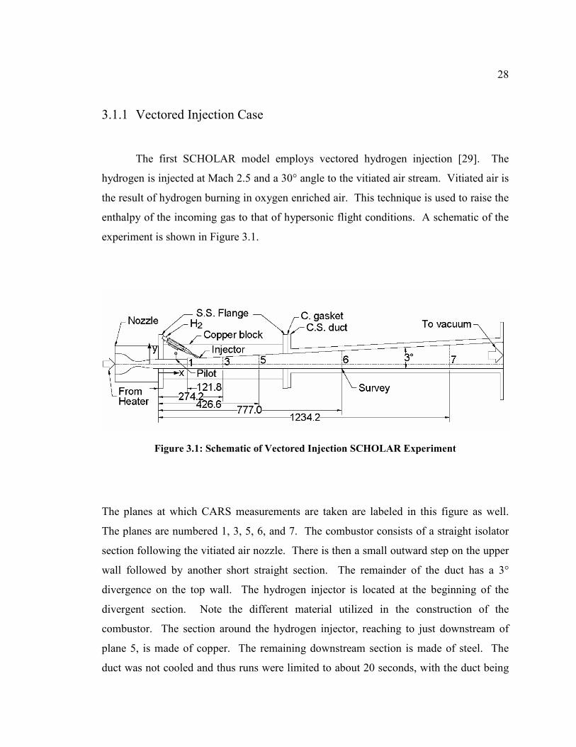
experiment is shown in Figure 3.1.

Figure 3.1: Schematic of Vectored Injection SCHOLAR Experiment

The planes at which CARS measurements are taken are labeled in this figure as well.

The planes are numbered 1, 3, 5, 6, and 7. The combustor consists of a straight isolator

section following the vitiated air nozzle. There is then a small outward step on the upper

wall followed by another short straight section. The remainder of the duct has a 3°

divergence on the top wall. The hydrogen injector is located at the beginning of the

divergent section. Note the different material utilized in the construction of the

combustor. The section around the hydrogen injector, reaching to just downstream of

plane 5, is made of copper. The remaining downstream section is made of steel. The

duct was not cooled and thus runs were limited to about 20 seconds, with the duct being

29

allowed to cool between runs. As a result of this, the wall temperatures are constantly

increasing with a rate depending on the location and local wall material. Measurements

are available for the wall temperatures as a function of time [11], but the simulation is not

time accurate, and thus these measurements cannot be used to provide a temperature

boundary condition. The specification of wall temperatures is discussed further in

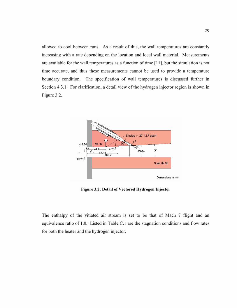
Section 4.3.1. For clarification, a detail view of the hydrogen injector region is shown in

Figure 3.2.

Figure 3.2: Detail of Vectored Hydrogen Injector

The enthalpy of the vitiated air stream is set to be that of Mach 7 flight and an

equivalence ratio of 1.0. Listed in Table C.1 are the stagnation conditions and flow rates

for both the heater and the hydrogen injector.

30

Table 3.1: Inflow Conditions for Vectored Injection

K4 302 eTemperatur1.0 of ratio

MPa0.065 3.44 Pressureeequivalenc tosCorrespond:Injector H

O kg/s 0.005 0.300

K75 1827 eTemperatur Hkg/s 0.0006 0.0284

MPa0.008 0.765 PressureAir kg/s 0.008 0.915:Heater

StagnationFlow RatesLocation

2

2

2

±

±

±

±±

±±

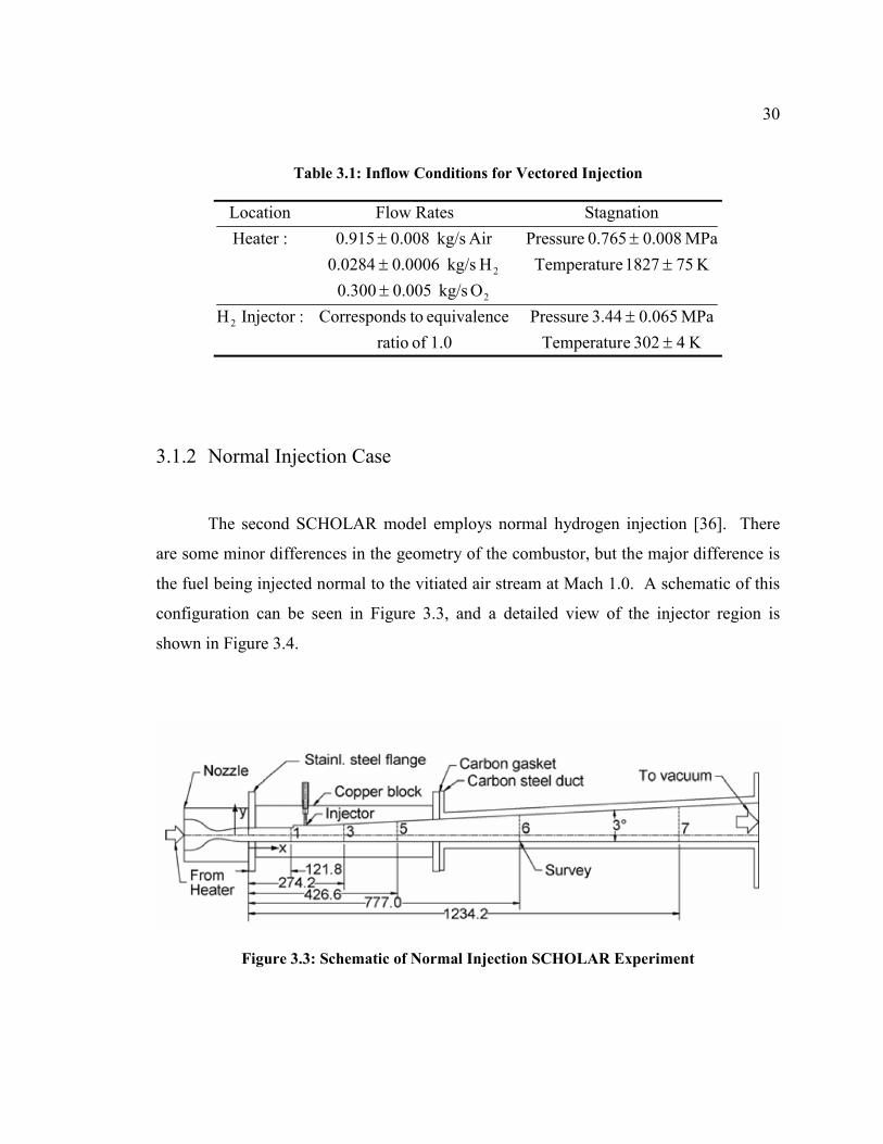
3.1.2 Normal Injection Case

The second SCHOLAR model employs normal hydrogen injection [36]. There

are some minor differences in the geometry of the combustor, but the major difference is

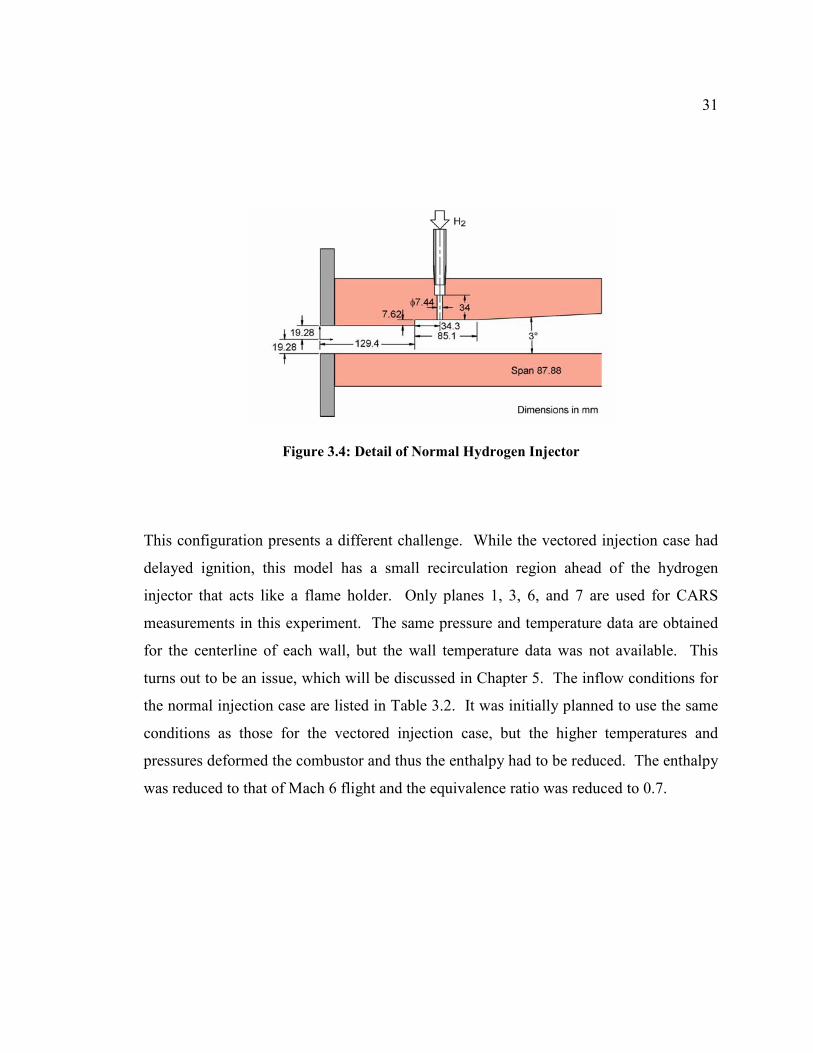
the fuel being injected normal to the vitiated air stream at Mach 1.0. A schematic of this

configuration can be seen in Figure 3.3, and a detailed view of the injector region is

shown in Figure 3.4.

Figure 3.3: Schematic of Normal Injection SCHOLAR Experiment

31

Figure 3.4: Detail of Normal Hydrogen Injector

This configuration presents a different challenge. While the vectored injection case had

delayed ignition, this model has a small recirculation region ahead of the hydrogen

injector that acts like a flame holder. Only planes 1, 3, 6, and 7 are used for CARS

measurements in this experiment. The same pressure and temperature data are obtained

for the centerline of each wall, but the wall temperature data was not available. This

turns out to be an issue, which will be discussed in Chapter 5. The inflow conditions for

the normal injection case are listed in Table 3.2. It was initially planned to use the same

conditions as those for the vectored injection case, but the higher temperatures and

pressures deformed the combustor and thus the enthalpy had to be reduced. The enthalpy

was reduced to that of Mach 6 flight and the equivalence ratio was reduced to 0.7.

32

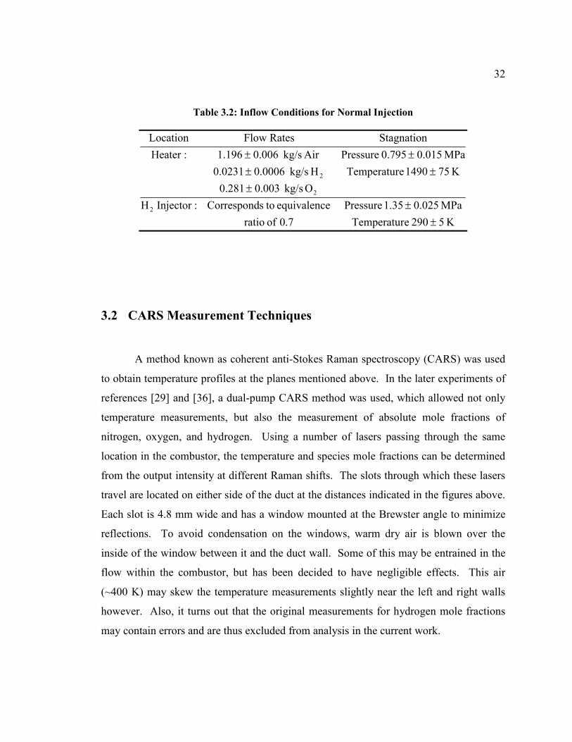
Table 3.2: Inflow Conditions for Normal Injection

K5 290 eTemperatur0.7 of ratio

MPa0.025 1.35 Pressureeequivalenc tosCorrespond:Injector H

O kg/s 0.003 0.281

K75 1490 eTemperatur Hkg/s 0.0006 0.0231

MPa0.015 0.795 PressureAir kg/s 0.006 1.196:Heater

StagnationFlow RatesLocation

2

2

2

±

±

±

±±

±±

3.2 CARS Measurement Techniques

A method known as coherent anti-Stokes Raman spectroscopy (CARS) was used

to obtain temperature profiles at the planes mentioned above. In the later experiments of

references [29] and [36], a dual-pump CARS method was used, which allowed not only

temperature measurements, but also the measurement of absolute mole fractions of

nitrogen, oxygen, and hydrogen. Using a number of lasers passing through the same

location in the combustor, the temperature and species mole fractions can be determined

from the output intensity at different Raman shifts. The slots through which these lasers

travel are located on either side of the duct at the distances indicated in the figures above.

Each slot is 4.8 mm wide and has a window mounted at the Brewster angle to minimize

reflections. To avoid condensation on the windows, warm dry air is blown over the

inside of the window between it and the duct wall. Some of this may be entrained in the

flow within the combustor, but has been decided to have negligible effects. This air

(~400 K) may skew the temperature measurements slightly near the left and right walls

however. Also, it turns out that the original measurements for hydrogen mole fractions

may contain errors and are thus excluded from analysis in the current work.

33

3.3 Experimental Data Fitting

Experimental data fitting is an important issue when comparing with CFD

simulations. The CARS data has a large amount of scatter, thus many measurements are

required to obtain spatially resolved averages. Because it is not practical to accumulate a

large sample, numerical techniques were used to smooth and present the data. A program

called Table Curve 3D® was used to generate the surface fits for the 2D array of data at

each plane. A large number of methods are available to generate these averages, many of

which are examined in reference [12] to determine the best option for the data that was

obtained. A preliminary CFD analysis was conducted in reference [13], and the methods

for comparison with computation and experiment were investigated in an attempt to

determine the best way to analyze the two sets of data. Figure 3.5 shows an example of

the CARS scatter data for temperature and the curve fit that has been applied to it. This

data represents a horizontal slice of plane 6 about half way between the top and bottom

walls (at y = 18.2 mm). This particular location is used throughout the current work for

comparison between experiment and computation. Similar plots are available for species

mole fractions.

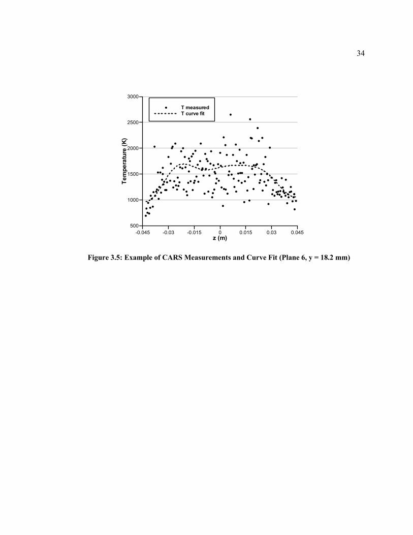
34

z (m)

Temperature(K)

-0.045 -0.03 -0.015 0 0.015 0.03 0.045

500

1000

1500

2000

2500

3000

T measured

T curve fit

Figure 3.5: Example of CARS Measurements and Curve Fit (Plane 6, y = 18.2 mm)

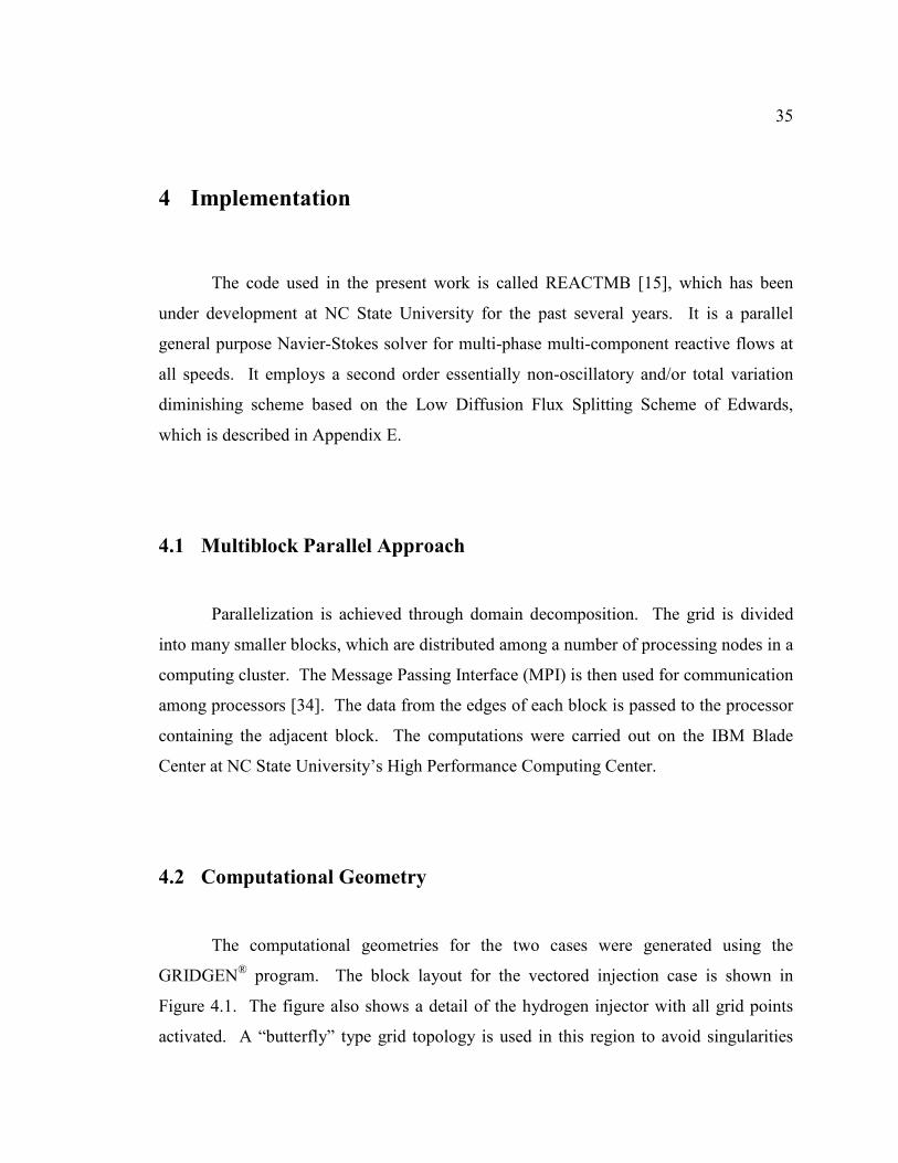
35

4 Implementation

The code used in the present work is called REACTMB [15], which has been

under development at NC State University for the past several years. It is a parallel

general purpose Navier-Stokes solver for multi-phase multi-component reactive flows at

all speeds. It employs a second order essentially non-oscillatory and/or total variation

diminishing scheme based on the Low Diffusion Flux Splitting Scheme of Edwards,

which is described in Appendix E.

4.1 Multiblock Parallel Approach

Parallelization is achieved through domain decomposition. The grid is divided

into many smaller blocks, which are distributed among a number of processing nodes in a

computing cluster. The Message Passing Interface (MPI) is then used for communication

among processors [34]. The data from the edges of each block is passed to the processor

containing the adjacent block. The computations were carried out on the IBM Blade

Center at NC State University’s High Performance Computing Center.

4.2 Computational Geometry

The computational geometries for the two cases were generated using the

GRIDGEN® program. The block layout for the vectored injection case is shown in

Figure 4.1. The figure also shows a detail of the hydrogen injector with all grid points

activated. A “butterfly” type grid topology is used in this region to avoid singularities

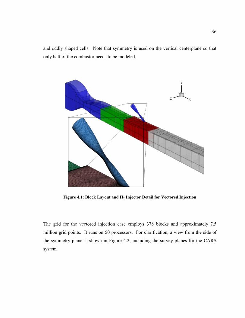
36

and oddly shaped cells. Note that symmetry is used on the vertical centerplane so that

only half of the combustor needs to be modeled.

Figure 4.1: Block Layout and H2 Injector Detail for Vectored Injection

The grid for the vectored injection case employs 378 blocks and approximately 7.5

million grid points. It runs on 50 processors. For clarification, a view from the side of

the symmetry plane is shown in Figure 4.2, including the survey planes for the CARS

system.

37

Figure 4.2: Vectored Block Layout with CARS Survey Planes Highlighted

The grid for the normal injection case is similar and was created by the same

means. The block layout for the normal injection case is shown in Figure 4.3.

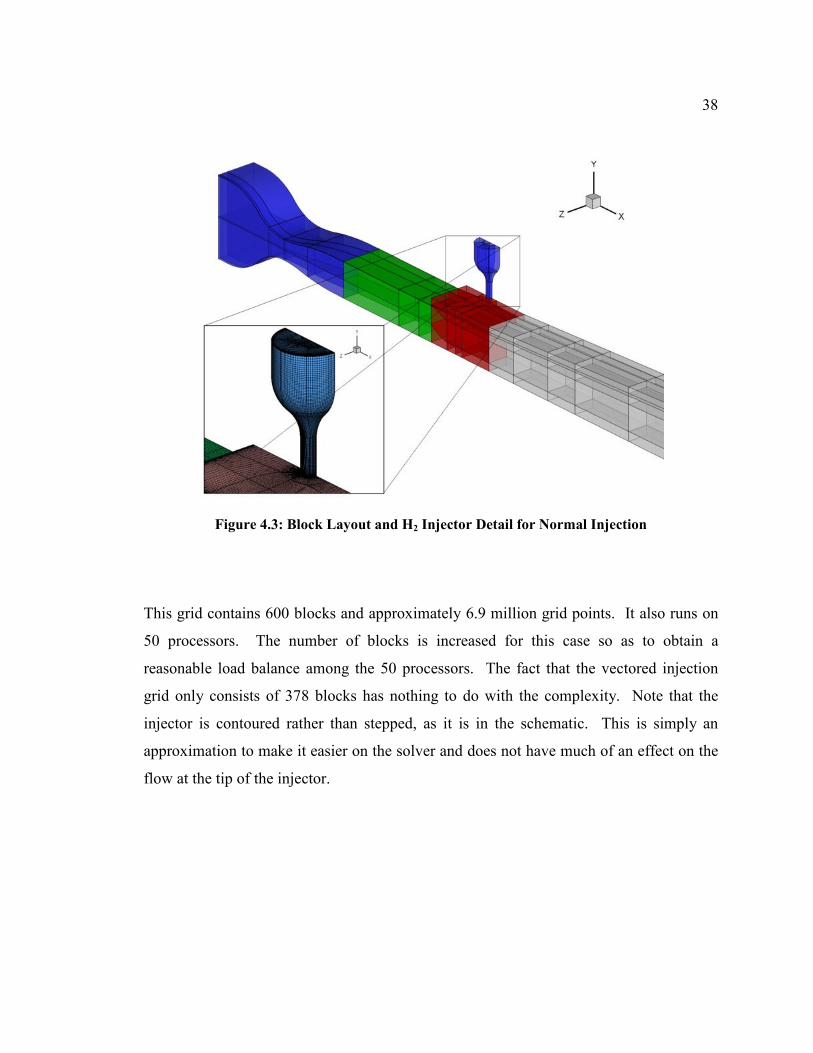
38

Figure 4.3: Block Layout and H2 Injector Detail for Normal Injection

This grid contains 600 blocks and approximately 6.9 million grid points. It also runs on

50 processors. The number of blocks is increased for this case so as to obtain a

reasonable load balance among the 50 processors. The fact that the vectored injection

grid only consists of 378 blocks has nothing to do with the complexity. Note that the

injector is contoured rather than stepped, as it is in the schematic. This is simply an

approximation to make it easier on the solver and does not have much of an effect on the

flow at the tip of the injector.

39

4.3 Wall and Inlet Boundary Conditions

For the representation of boundary conditions, the ghost cell method is employed.

Rather than imposing boundary conditions directly on the fluxes at a wall or inlet, an

imaginary cell on the opposite side of the boundary is created. The data in these cells is

defined in a way such that the flux at the interface between them corresponds to the

physical boundary conditions, such as the no-slip velocity condition and constant or

adiabatic wall temperature. When higher order flux reconstruction schemes are used,

multiple layers of cells may be required. The code can accommodate up to three layers

of ghost cells. Since symmetry is utilized, a symmetry boundary condition is necessary.

This is achieved by merely mirroring all scalar properties into the ghost cells from the

interior cells. Care must be taken with the velocity vector however. Since the plane is of

constant z, the w velocity component must be made negative. The other components are

simply copied.

4.3.1 Wall Boundaries

A number of different wall boundary conditions are required for the present

simulation. The first condition corresponds to the no-slip condition.

0=== www wvu (4.1)

0=∂∂

wn

p (4.2)

The direction normal to the wall is represented by n. The velocities become zero at the

wall by applying the negative of all three velocity components to the ghost cells. The

zero pressure gradient is enforced by simply setting the ghost cell pressure to the nearest

internal cell pressure. Higher order approximations of this are also possible.

40

For the species equations, the normal concentration gradient must be zero at the

wall.

0=∂∂

w

m

n

Y (4.3)

This is enforced in a manner similar to the pressure.

There are various options for the wall temperature. The first and simplest

condition is an adiabatic wall. Since the heat flux is proportional to the temperature

gradient, the normal temperature gradient at the wall must be zero for it to be adiabatic.

Conditions similar to the pressure and mass fractions can be used for this. The second

possibility is to have an isothermal wall, meaning that the temperature is constant. To

accomplish this, the temperature is extrapolated from the first internal layer of cells

through the wall into the ghost cell. Many times this can result in a negative temperature

in the ghost cell. This of course must be limited to a small positive value, or the

calculation of the viscosity or other thermal properties in that cell will cause the program

to crash. A third option is the isothermal ghost cell wall. This is somewhere between an

adiabatic wall and an isothermal wall. The wall temperature is allowed to change but still

remains close to the specified ghost cell value.

For the turbulence model, k = 0 at the walls. For ζ, the wall condition reduces to

the following.

w

wn

k

n

∂∂

∂∂

= ννζ (4.4)

The boundary conditions for the variable turbulent Prandtl/Schmidt number models are

similar to those of the k-ζ model. σY and ~2h ′′ must be zero at the walls, and a condition

similar to Equation (4.4) holds for the dissipation rates.

41

4.3.2 Inflow and Outflow Boundaries

Both of the inflow boundaries, the vitiated air nozzle and the hydrogen nozzle, are

subsonic. With grid aligned subsonic flow, there is one characteristic that propagates

backward, out of the domain. For this reason, some information must be extrapolated

from the flow inside the boundary. The velocity components are best suited for this. For

the k-ζ turbulence model, the incoming turbulence intensity Tu and the initial length scale

(νt / ν) must be specified.

The outflow boundary is supersonic for this combustor; therefore all

characteristics are propagating out of the domain. This means that the entire solution

must be extrapolated into the ghost cells.

42

5 Results and Discussion

This chapter presents the results that have been obtained using the procedures and

models described in the previous sections for both the vectored injection experiment and

the normal injection experiment. Below is a list of the important factors investigated in

this work.

• Wall temperatures and thermal boundary conditions. Since the walls were not

cooled, a variety of methods were investigated.

• Specification of various inflow conditions such as turbulence intensity, length

scale (νt / ν), and OH concentration.

• Grid resolution and refinement for the vectored injection case.

• Role of software in comparing computed data with experimental data.

• Variable vs. constant turbulent Prandtl/Schmidt numbers.

• Role of chemical kinetic mechanisms.

• Role of the compressibility term.

5.1 General Results

As mentioned above, one of the factors investigated was the effect of the inflow

conditions on the solution. The sensitivities of several parameters were examined. First

is the initial turbulence intensity, which is defined as:

23

2100

∞

∞=u

kTu (5.1)

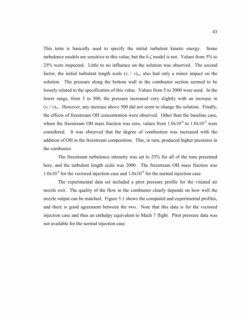
43

This term is basically used to specify the initial turbulent kinetic energy. Some

turbulence models are sensitive to this value, but the k-ζ model is not. Values from 5% to

25% were inspected. Little to no influence on the solution was observed. The second

factor, the initial turbulent length scale (νt / ν)∞, also had only a minor impact on the

solution. The pressure along the bottom wall in the combustor section seemed to be

loosely related to the specification of this value. Values from 5 to 2000 were used. In the

lower range, from 5 to 500, the pressure increased very slightly with an increase in

(νt / ν)∞. However, any increase above 500 did not seem to change the solution. Finally,

the effects of freestream OH concentration were observed. Other than the baseline case,

where the freestream OH mass fraction was zero, values from 1.0x10-6 to 1.0x10

-3 were

considered. It was observed that the degree of combustion was increased with the

addition of OH in the freestream composition. This, in turn, produced higher pressures in

the combustor.

The freestream turbulence intensity was set to 25% for all of the runs presented

here, and the turbulent length scale was 2000. The freestream OH mass fraction was

1.0x10-5 for the vectored injection case and 1.0x10

-6 for the normal injection case.

The experimental data set included a pitot pressure profile for the vitiated air

nozzle exit. The quality of the flow in the combustor clearly depends on how well the

nozzle output can be matched. Figure 5.1 shows the computed and experimental profiles,

and there is good agreement between the two. Note that this data is for the vectored

injection case and thus an enthalpy equivalent to Mach 7 flight. Pitot pressure data was

not available for the normal injection case.

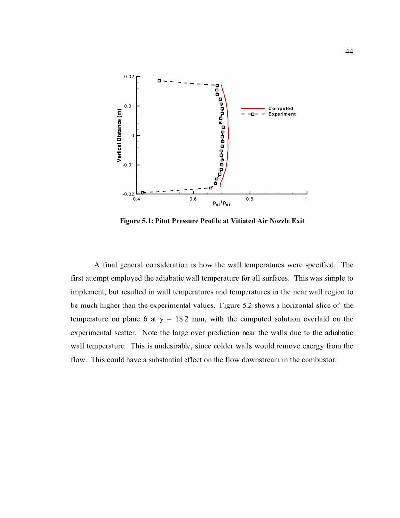
44

p02/p01

VerticalDistance(m)

0.4 0.6 0.8 1

-0.02

-0.01

0

0.01

0.02

Computed

Experiment

Figure 5.1: Pitot Pressure Profile at Vitiated Air Nozzle Exit

A final general consideration is how the wall temperatures were specified. The

first attempt employed the adiabatic wall temperature for all surfaces. This was simple to

implement, but resulted in wall temperatures and temperatures in the near wall region to

be much higher than the experimental values. Figure 5.2 shows a horizontal slice of the

temperature on plane 6 at y = 18.2 mm, with the computed solution overlaid on the

experimental scatter. Note the large over prediction near the walls due to the adiabatic

wall temperature. This is undesirable, since colder walls would remove energy from the

flow. This could have a substantial effect on the flow downstream in the combustor.

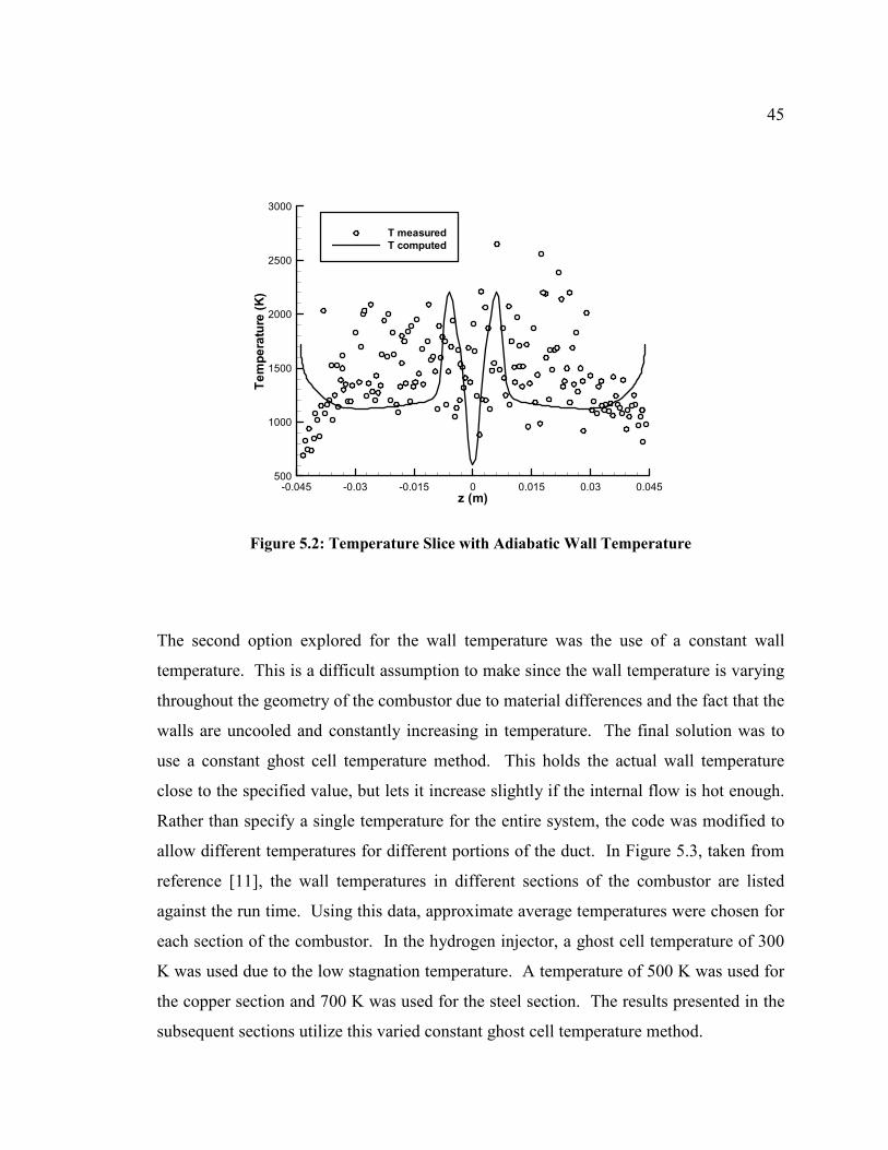
45

z (m)

Temperature(K)

-0.045 -0.03 -0.015 0 0.015 0.03 0.045

500

1000

1500

2000

2500

3000

T measured

T computed

Figure 5.2: Temperature Slice with Adiabatic Wall Temperature

The second option explored for the wall temperature was the use of a constant wall

temperature. This is a difficult assumption to make since the wall temperature is varying

throughout the geometry of the combustor due to material differences and the fact that the

walls are uncooled and constantly increasing in temperature. The final solution was to

use a constant ghost cell temperature method. This holds the actual wall temperature

close to the specified value, but lets it increase slightly if the internal flow is hot enough.

Rather than specify a single temperature for the entire system, the code was modified to

allow different temperatures for different portions of the duct. In Figure 5.3, taken from

reference [11], the wall temperatures in different sections of the combustor are listed

against the run time. Using this data, approximate average temperatures were chosen for

each section of the combustor. In the hydrogen injector, a ghost cell temperature of 300

K was used due to the low stagnation temperature. A temperature of 500 K was used for

the copper section and 700 K was used for the steel section. The results presented in the

subsequent sections utilize this varied constant ghost cell temperature method.

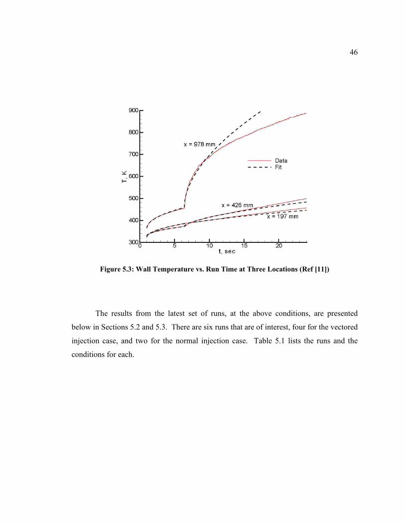
46

Figure 5.3: Wall Temperature vs. Run Time at Three Locations (Ref [11])

The results from the latest set of runs, at the above conditions, are presented

below in Sections 5.2 and 5.3. There are six runs that are of interest, four for the vectored

injection case, and two for the normal injection case. Table 5.1 lists the runs and the

conditions for each.

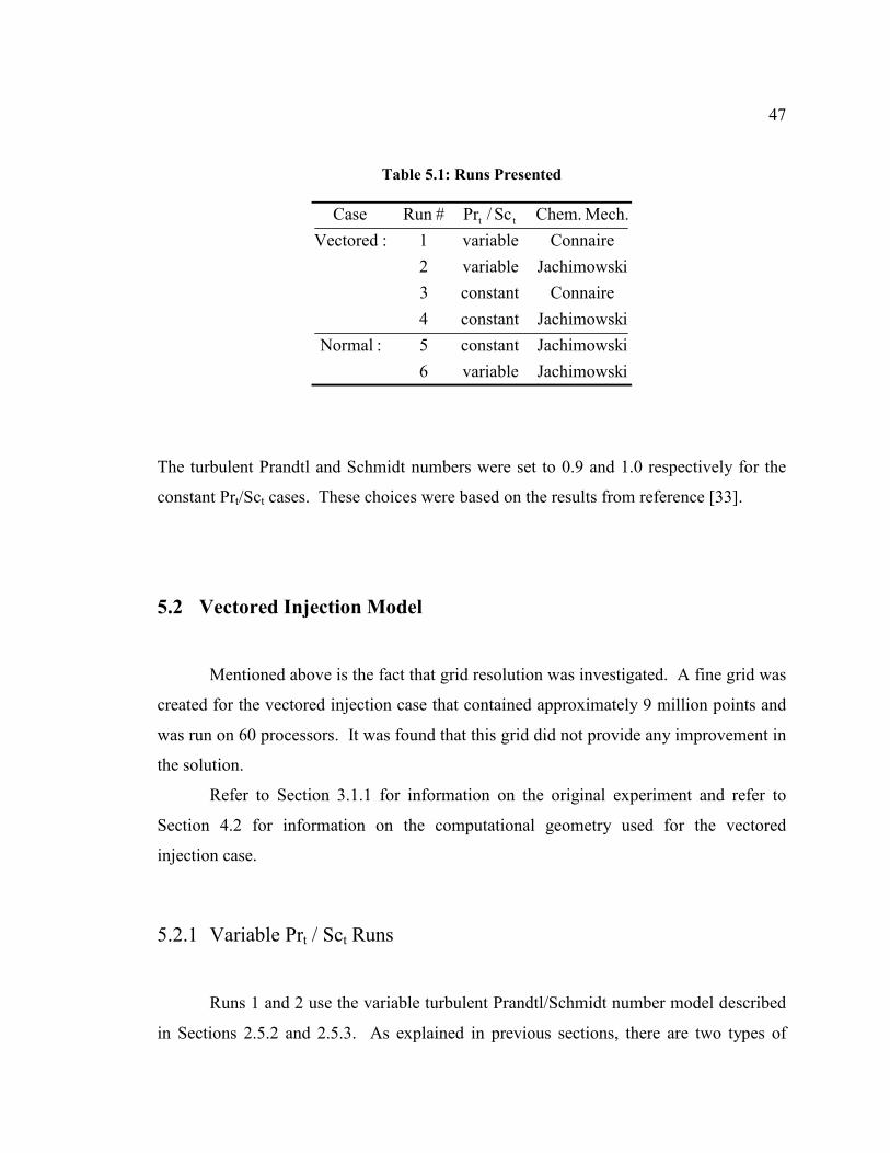
47

Table 5.1: Runs Presented

iJachimowskvariable6

iJachimowskconstant5:Normal

iJachimowskconstant4

Connaireconstant3

iJachimowskvariable2

Connairevariable1:Vectored

Mech.Chem.Sc/Pr# RunCase tt

The turbulent Prandtl and Schmidt numbers were set to 0.9 and 1.0 respectively for the

constant Prt/Sct cases. These choices were based on the results from reference [33].

5.2 Vectored Injection Model

Mentioned above is the fact that grid resolution was investigated. A fine grid was

created for the vectored injection case that contained approximately 9 million points and

was run on 60 processors. It was found that this grid did not provide any improvement in

the solution.

Refer to Section 3.1.1 for information on the original experiment and refer to

Section 4.2 for information on the computational geometry used for the vectored

injection case.

5.2.1 Variable Prt / Sct Runs

Runs 1 and 2 use the variable turbulent Prandtl/Schmidt number model described

in Sections 2.5.2 and 2.5.3. As explained in previous sections, there are two types of

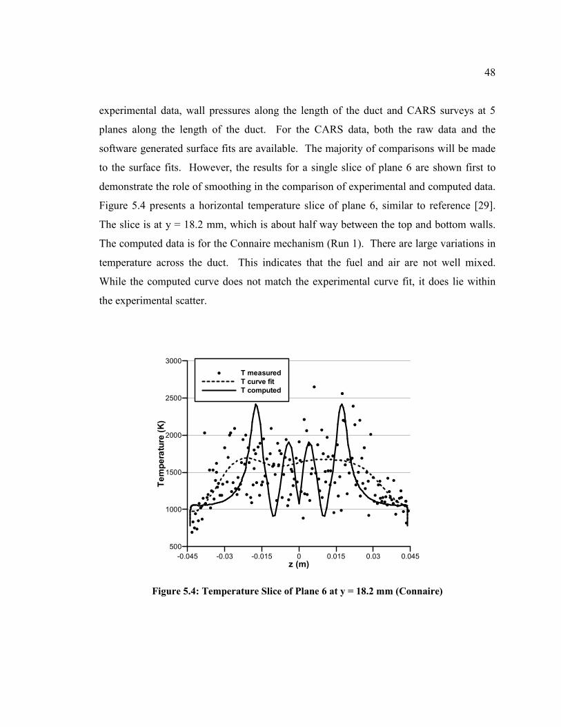
48

experimental data, wall pressures along the length of the duct and CARS surveys at 5

planes along the length of the duct. For the CARS data, both the raw data and the

software generated surface fits are available. The majority of comparisons will be made

to the surface fits. However, the results for a single slice of plane 6 are shown first to

demonstrate the role of smoothing in the comparison of experimental and computed data.

Figure 5.4 presents a horizontal temperature slice of plane 6, similar to reference [29].

The slice is at y = 18.2 mm, which is about half way between the top and bottom walls.

The computed data is for the Connaire mechanism (Run 1). There are large variations in

temperature across the duct. This indicates that the fuel and air are not well mixed.

While the computed curve does not match the experimental curve fit, it does lie within

the experimental scatter.

z (m)

Temperature(K)

-0.045 -0.03 -0.015 0 0.015 0.03 0.045

500

1000

1500

2000

2500

3000

T measured

T curve fit

T computed

Figure 5.4: Temperature Slice of Plane 6 at y = 18.2 mm (Connaire)

49

Figure 5.5 shows nitrogen and oxygen mole fraction slices at the same location. The

profiles follow the same trends as the experimental data, but again, do not follow the

curve fit applied to the experimental data.

z (m)

MoleFraction

-0.045 -0.03 -0.015 0 0.015 0.03 0.045

0

0.1

0.2

0.3

0.4

0.5

0.6

0.7

0.8

0.9

N2 measured

N2 curve fit

N2 computed

z (m)

MoleFraction

-0.045 -0.03 -0.015 0 0.015 0.03 0.045

-0.1

0

0.1

0.2

0.3

0.4

O2 measured

O2 curve fit

O2 computed

Figure 5.5: Mole Fraction Slices of Plane 6 at y = 18.2 mm (Connaire)

In an effort to obtain a more reasonable comparison between computed and

experimental data, the same curve fit was applied to both sets of data. Figure 5.6 shows

the same slice as Figure 5.4, but with a 5th degree polynomial fit applied to both the raw

experimental data and the computed solution. A 5th degree polynomial was chosen since,

when applied to the experimental scatter, it most closely resembled the original curve fit,

which is also shown in the figure for reference. Clearly, when subjected to the same

smoothing, the computed solution displays very good agreement with the experimental

data. Similar results are seen for the nitrogen and oxygen mole fractions, shown in

Figure 5.7. The Jachimowski mechanism provides similar results.

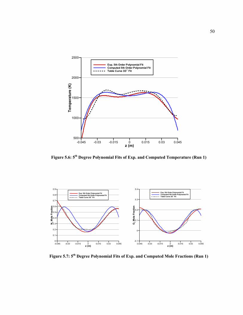
50

z (m)

Temperature(K)

-0.045 -0.03 -0.015 0 0.015 0.03 0.045

500

1000

1500

2000

2500

Exp. 5th Order Polynomial Fit

Computed 5th Order Polynomial Fit

Table Curve 3DFit

Figure 5.6: 5th Degree Polynomial Fits of Exp. and Computed Temperature (Run 1)

z (m)

N2MoleFraction

-0.045 -0.03 -0.015 0 0.015 0.03 0.045

0

0.1

0.2

0.3

0.4

0.5

0.6

0.7

0.8

0.9

Exp. 5th Order Polynomial Fit

Computed 5th Order Polynomial Fit

Table Curve 3DFit

z (m)

O2MoleFraction

-0.045 -0.03 -0.015 0 0.015 0.03 0.045

-0.1

0

0.1

0.2

0.3

0.4

Exp. 5th Order Polynomial Fit

Computed 5th Order Polynomial Fit

Table Curve 3DFit

Figure 5.7: 5th Degree Polynomial Fits of Exp. and Computed Mole Fractions (Run 1)

51

Figure 5.8 shows the CARS surface fits of temperature for the vectored injection

model. Regardless of the fact that the data is slightly asymmetric, the computed results

are shown on the left side of each slice and the experimental data on the right side. The

temperature contours for the Connaire mechanism (Run 1) plotted against the smoothed

experimental data are shown in Figure 5.9. Note the thin combustion region as opposed

to the smoothed experimental data. Also, there is indication of ignition on plane 5 for the

computed solution that is not reflected in the experimental data.

Figure 5.8: Experimental Surface Fits of Temperature for Vectored Case

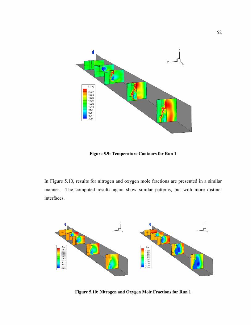
52

Figure 5.9: Temperature Contours for Run 1

In Figure 5.10, results for nitrogen and oxygen mole fractions are presented in a similar

manner. The computed results again show similar patterns, but with more distinct

interfaces.

Figure 5.10: Nitrogen and Oxygen Mole Fractions for Run 1

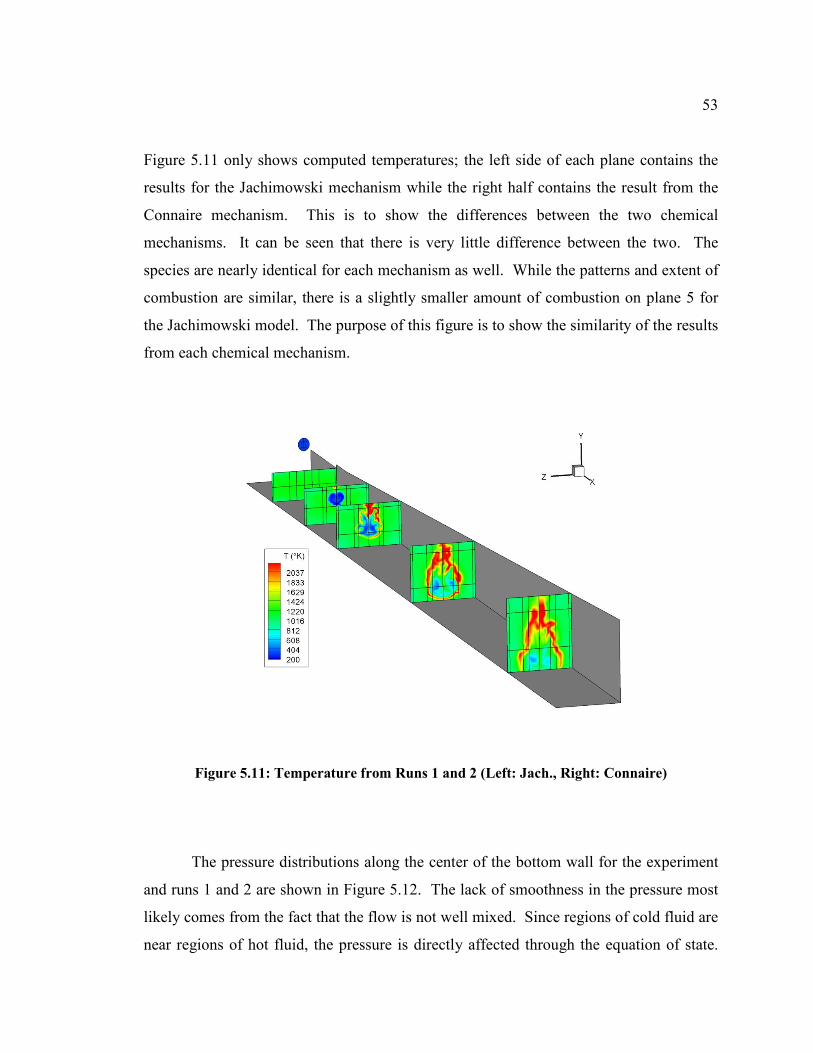
53

Figure 5.11 only shows computed temperatures; the left side of each plane contains the

results for the Jachimowski mechanism while the right half contains the result from the

Connaire mechanism. This is to show the differences between the two chemical

mechanisms. It can be seen that there is very little difference between the two. The

species are nearly identical for each mechanism as well. While the patterns and extent of

combustion are similar, there is a slightly smaller amount of combustion on plane 5 for

the Jachimowski model. The purpose of this figure is to show the similarity of the results

from each chemical mechanism.

Figure 5.11: Temperature from Runs 1 and 2 (Left: Jach., Right: Connaire)

The pressure distributions along the center of the bottom wall for the experiment

and runs 1 and 2 are shown in Figure 5.12. The lack of smoothness in the pressure most

likely comes from the fact that the flow is not well mixed. Since regions of cold fluid are

near regions of hot fluid, the pressure is directly affected through the equation of state.

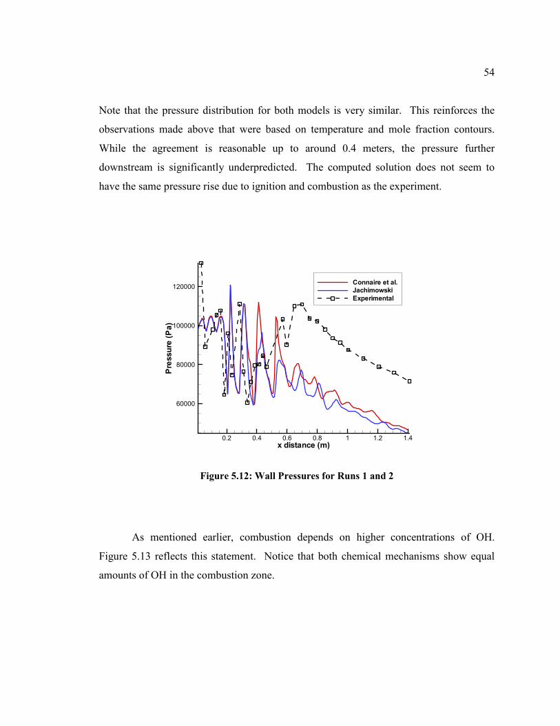
54

Note that the pressure distribution for both models is very similar. This reinforces the

observations made above that were based on temperature and mole fraction contours.

While the agreement is reasonable up to around 0.4 meters, the pressure further

downstream is significantly underpredicted. The computed solution does not seem to

have the same pressure rise due to ignition and combustion as the experiment.

x distance (m)

Pressure(Pa)

0.2 0.4 0.6 0.8 1 1.2 1.4

60000

80000

100000

120000Connaire et al.

Jachimowski

Experimental

Figure 5.12: Wall Pressures for Runs 1 and 2

As mentioned earlier, combustion depends on higher concentrations of OH.

Figure 5.13 reflects this statement. Notice that both chemical mechanisms show equal

amounts of OH in the combustion zone.

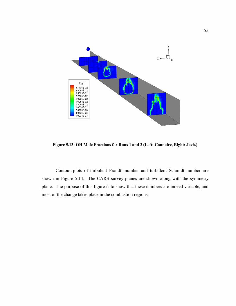
55

Figure 5.13: OH Mole Fractions for Runs 1 and 2 (Left: Connaire, Right: Jach.)

Contour plots of turbulent Prandtl number and turbulent Schmidt number are

shown in Figure 5.14. The CARS survey planes are shown along with the symmetry

plane. The purpose of this figure is to show that these numbers are indeed variable, and

most of the change takes place in the combustion regions.

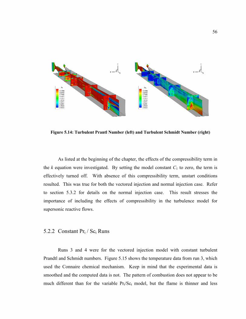
56

Figure 5.14: Turbulent Prantl Number (left) and Turbulent Schmidt Number (right)

As listed at the beginning of the chapter, the effects of the compressibility term in

the k equation were investigated. By setting the model constant C1 to zero, the term is

effectively turned off. With absence of this compressibility term, unstart conditions

resulted. This was true for both the vectored injection and normal injection case. Refer

to section 5.3.2 for details on the normal injection case. This result stresses the

importance of including the effects of compressibility in the turbulence model for

supersonic reactive flows.

5.2.2 Constant Prt / Sct Runs

Runs 3 and 4 were for the vectored injection model with constant turbulent

Prandtl and Schmidt numbers. Figure 5.15 shows the temperature data from run 3, which

used the Connaire chemical mechanism. Keep in mind that the experimental data is

smoothed and the computed data is not. The pattern of combustion does not appear to be

much different than for the variable Prt/Sct model, but the flame is thinner and less

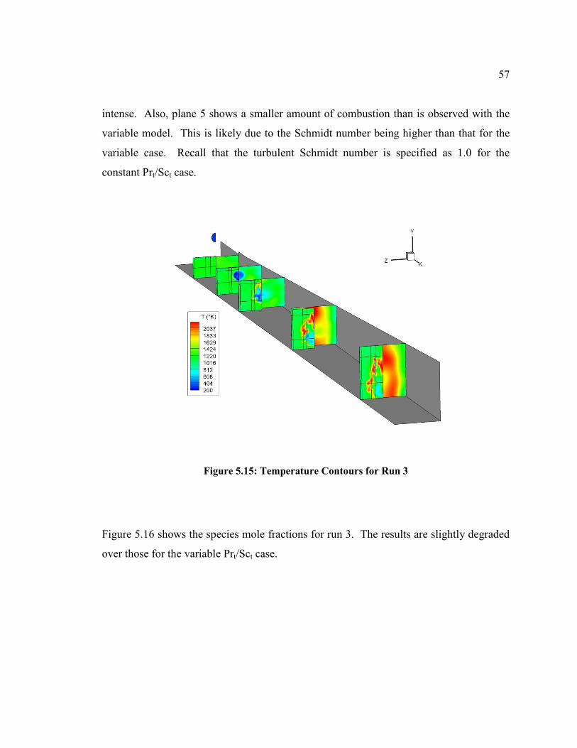
57

intense. Also, plane 5 shows a smaller amount of combustion than is observed with the

variable model. This is likely due to the Schmidt number being higher than that for the

variable case. Recall that the turbulent Schmidt number is specified as 1.0 for the

constant Prt/Sct case.

Figure 5.15: Temperature Contours for Run 3

Figure 5.16 shows the species mole fractions for run 3. The results are slightly degraded

over those for the variable Prt/Sct case.

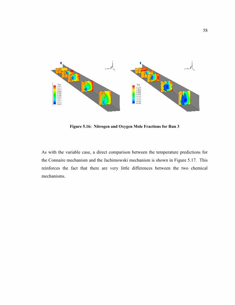
58

Figure 5.16: Nitrogen and Oxygen Mole Fractions for Run 3

As with the variable case, a direct comparison between the temperature predictions for

the Connaire mechanism and the Jachimowski mechanism is shown in Figure 5.17. This

reinforces the fact that there are very little differences between the two chemical

mechanisms.

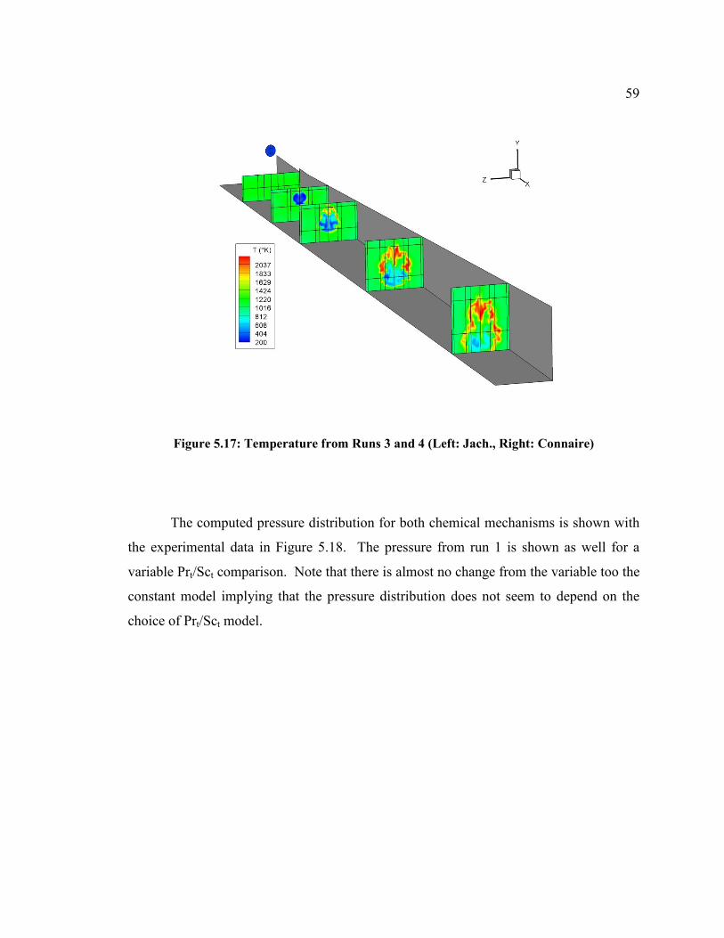
59

Figure 5.17: Temperature from Runs 3 and 4 (Left: Jach., Right: Connaire)

The computed pressure distribution for both chemical mechanisms is shown with

the experimental data in Figure 5.18. The pressure from run 1 is shown as well for a

variable Prt/Sct comparison. Note that there is almost no change from the variable too the

constant model implying that the pressure distribution does not seem to depend on the

choice of Prt/Sct model.

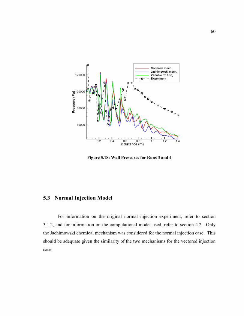
60

x distance (m)

Pressure(Pa)

0.2 0.4 0.6 0.8 1 1.2 1.4

60000

80000

100000

120000

Connaire mech.

Jachimowski mech.

Variable Prt/ Sc

t

Experiment

Figure 5.18: Wall Pressures for Runs 3 and 4

5.3 Normal Injection Model

For information on the original normal injection experiment, refer to section

3.1.2, and for information on the computational model used, refer to section 4.2. Only

the Jachimowski chemical mechanism was considered for the normal injection case. This

should be adequate given the similarity of the two mechanisms for the vectored injection

case.

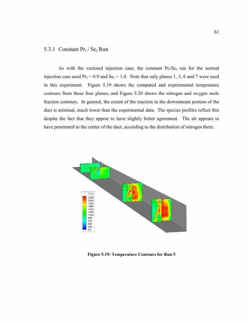
61

5.3.1 Constant Prt / Sct Run

As with the vectored injection case, the constant Prt/Sct run for the normal

injection case used Prt = 0.9 and Sct = 1.0. Note that only planes 1, 3, 6 and 7 were used

in this experiment. Figure 5.19 shows the computed and experimental temperature

contours from these four planes, and Figure 5.20 shows the nitrogen and oxygen mole

fraction contours. In general, the extent of the reaction in the downstream portion of the

duct is minimal, much lower than the experimental data. The species profiles reflect this

despite the fact that they appear to have slightly better agreement. The air appears to

have penetrated to the center of the duct, according to the distribution of nitrogen there.

Figure 5.19: Temperature Contours for Run 5

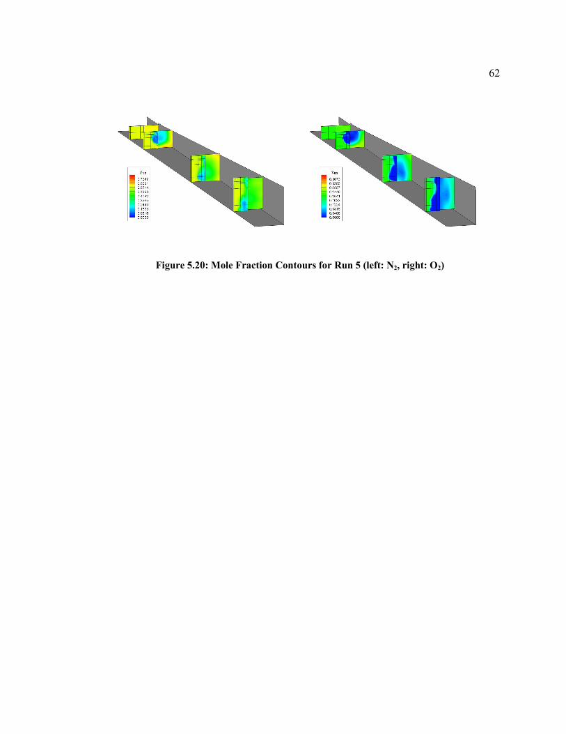
62

Figure 5.20: Mole Fraction Contours for Run 5 (left: N2, right: O2)

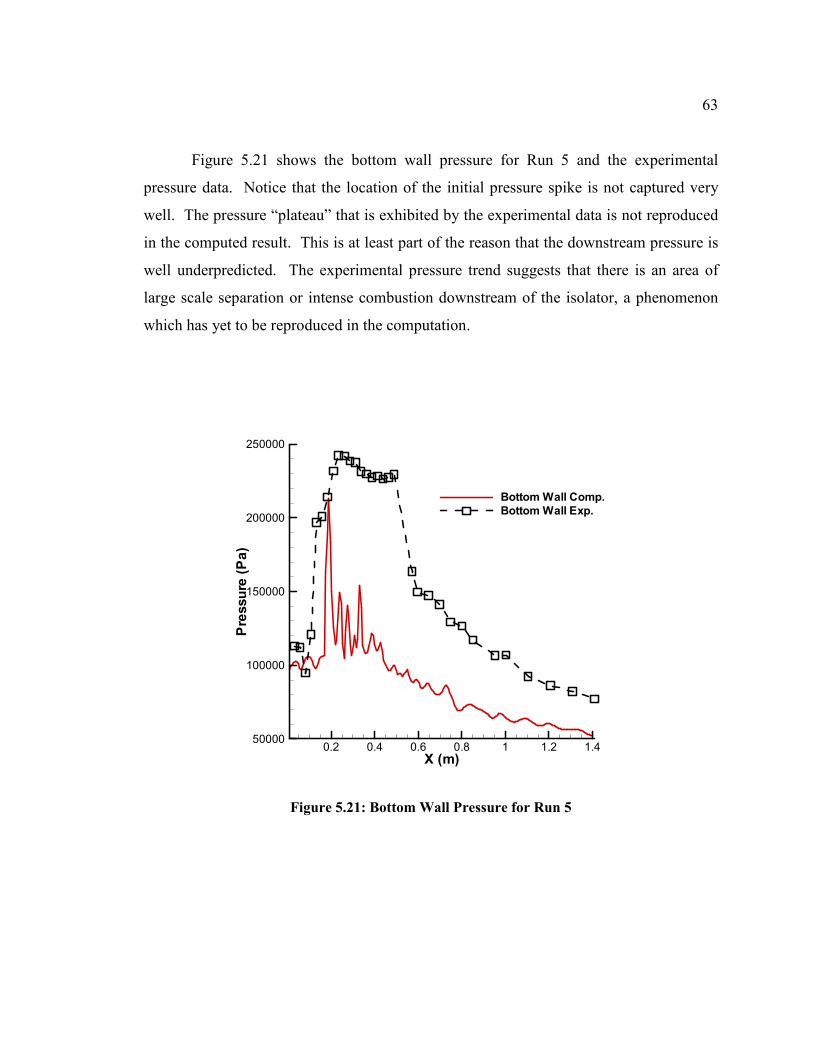
63

Figure 5.21 shows the bottom wall pressure for Run 5 and the experimental

pressure data. Notice that the location of the initial pressure spike is not captured very

well. The pressure “plateau” that is exhibited by the experimental data is not reproduced

in the computed result. This is at least part of the reason that the downstream pressure is

well underpredicted. The experimental pressure trend suggests that there is an area of

large scale separation or intense combustion downstream of the isolator, a phenomenon

which has yet to be reproduced in the computation.

X (m)

Pressure(Pa)

0.2 0.4 0.6 0.8 1 1.2 1.450000

100000

150000

200000

250000

Bottom Wall Comp.

Bottom Wall Exp.

Figure 5.21: Bottom Wall Pressure for Run 5

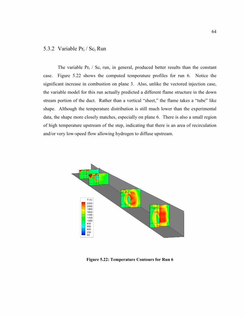
64

5.3.2 Variable Prt / Sct Run

The variable Prt / Sct run, in general, produced better results than the constant

case. Figure 5.22 shows the computed temperature profiles for run 6. Notice the

significant increase in combustion on plane 3. Also, unlike the vectored injection case,

the variable model for this run actually predicted a different flame structure in the down

stream portion of the duct. Rather than a vertical “sheet,” the flame takes a “tube” like

shape. Although the temperature distribution is still much lower than the experimental

data, the shape more closely matches, especially on plane 6. There is also a small region

of high temperature upstream of the step, indicating that there is an area of recirculation

and/or very low-speed flow allowing hydrogen to diffuse upstream.

Figure 5.22: Temperature Contours for Run 6

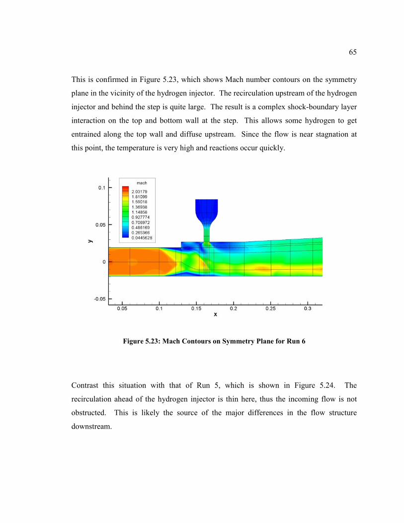
65

This is confirmed in Figure 5.23, which shows Mach number contours on the symmetry

plane in the vicinity of the hydrogen injector. The recirculation upstream of the hydrogen

injector and behind the step is quite large. The result is a complex shock-boundary layer

interaction on the top and bottom wall at the step. This allows some hydrogen to get

entrained along the top wall and diffuse upstream. Since the flow is near stagnation at

this point, the temperature is very high and reactions occur quickly.

Figure 5.23: Mach Contours on Symmetry Plane for Run 6

Contrast this situation with that of Run 5, which is shown in Figure 5.24. The

recirculation ahead of the hydrogen injector is thin here, thus the incoming flow is not

obstructed. This is likely the source of the major differences in the flow structure

downstream.

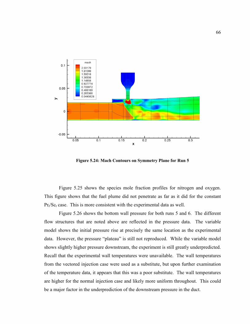
66

Figure 5.24: Mach Contours on Symmetry Plane for Run 5

Figure 5.25 shows the species mole fraction profiles for nitrogen and oxygen.

This figure shows that the fuel plume did not penetrate as far as it did for the constant

Prt/Sct case. This is more consistent with the experimental data as well.

Figure 5.26 shows the bottom wall pressure for both runs 5 and 6. The different

flow structures that are noted above are reflected in the pressure data. The variable

model shows the initial pressure rise at precisely the same location as the experimental

data. However, the pressure “plateau” is still not reproduced. While the variable model

shows slightly higher pressure downstream, the experiment is still greatly underpredicted.

Recall that the experimental wall temperatures were unavailable. The wall temperatures

from the vectored injection case were used as a substitute, but upon further examination

of the temperature data, it appears that this was a poor substitute. The wall temperatures

are higher for the normal injection case and likely more uniform throughout. This could

be a major factor in the underprediction of the downstream pressure in the duct.

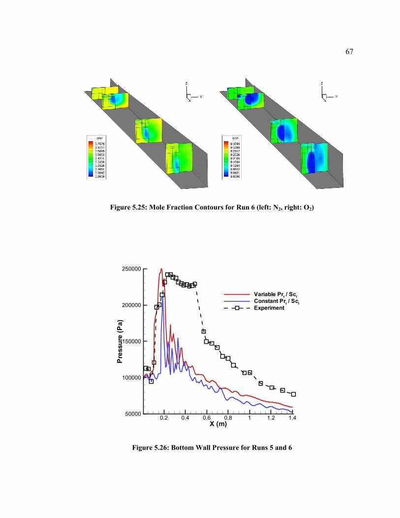
67

Figure 5.25: Mole Fraction Contours for Run 6 (left: N2, right: O2)

X (m)

Pressure(Pa)

0.2 0.4 0.6 0.8 1 1.2 1.450000

100000

150000

200000

250000

Variable Prt/ Sc

t

Constant Prt/ Sc

t

Experiment

Figure 5.26: Bottom Wall Pressure for Runs 5 and 6

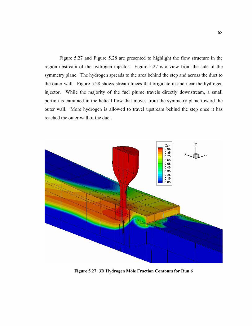
68

Figure 5.27 and Figure 5.28 are presented to highlight the flow structure in the

region upstream of the hydrogen injector. Figure 5.27 is a view from the side of the

symmetry plane. The hydrogen spreads to the area behind the step and across the duct to

the outer wall. Figure 5.28 shows stream traces that originate in and near the hydrogen

injector. While the majority of the fuel plume travels directly downstream, a small

portion is entrained in the helical flow that moves from the symmetry plane toward the

outer wall. More hydrogen is allowed to travel upstream behind the step once it has

reached the outer wall of the duct.

Figure 5.27: 3D Hydrogen Mole Fraction Contours for Run 6

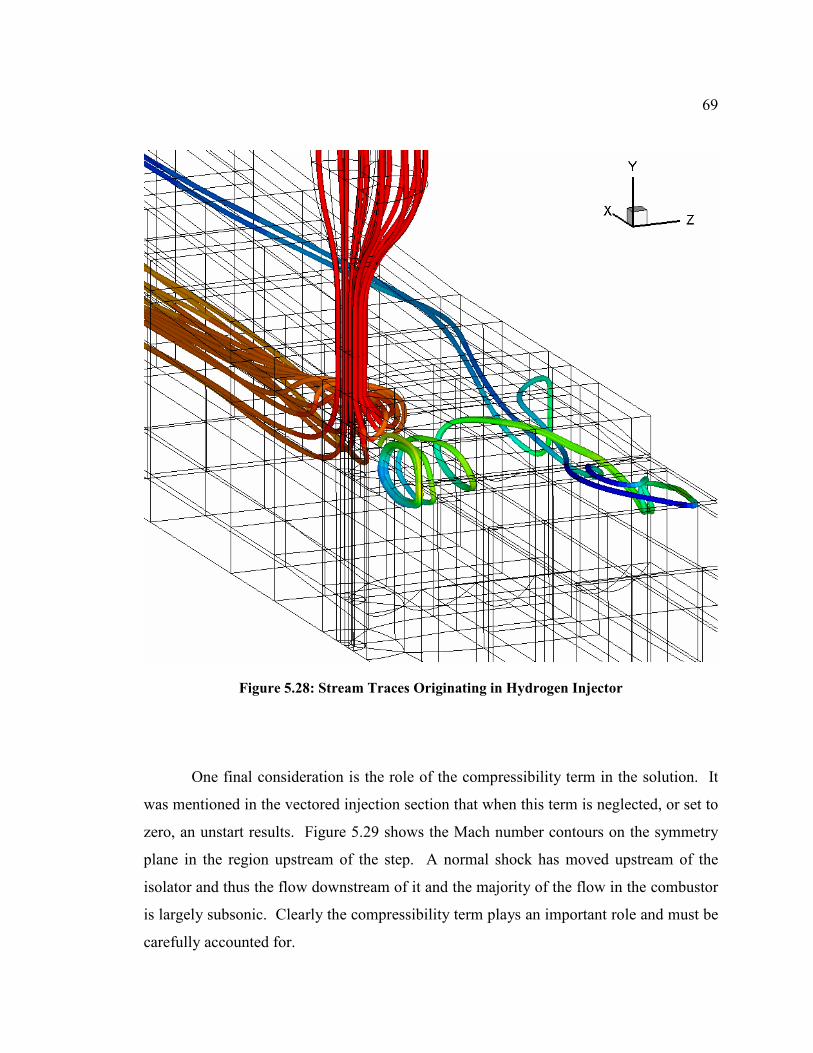
69

Figure 5.28: Stream Traces Originating in Hydrogen Injector

One final consideration is the role of the compressibility term in the solution. It

was mentioned in the vectored injection section that when this term is neglected, or set to

zero, an unstart results. Figure 5.29 shows the Mach number contours on the symmetry

plane in the region upstream of the step. A normal shock has moved upstream of the

isolator and thus the flow downstream of it and the majority of the flow in the combustor

is largely subsonic. Clearly the compressibility term plays an important role and must be

carefully accounted for.

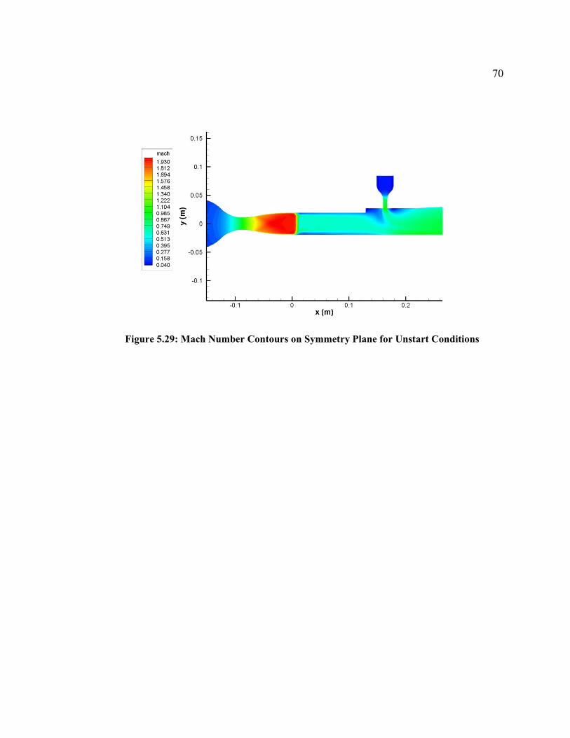
70

Figure 5.29: Mach Number Contours on Symmetry Plane for Unstart Conditions

71

6 Conclusions

The turbulence model employed in the current work removes uncertainties in

specifying the turbulent Prandtl and Schmidt numbers. Classic turbulence models

assume these numbers to be constant and they must be specified before hand. In reality,

these numbers are not constant for complex three dimensional flows, and the chosen

values can have profound effects on the solution. The model also accounts for

turbulence/chemistry interactions, which are certainly necessary for scramjet type flows.

Also, an item which has received little attention in the literature is the role of the

compressibility correction in the turbulence model. The current results show that

neglecting this term results in an unstart condition for this specific experiment. Despite

these efforts to improve the modeling, the prediction of ignition location is still difficult.

Other factors such as grid resolution and chemical kinetic models can also have a

profound effect on ignition location.

In general, the current model shows early ignition and a lack of significant

combustion downstream. Even so, the computed temperature profiles do fall within

experimental scatter, and when subjected to the same curve fits, the two show very good

agreement. This stresses the fact that care must be taken when comparing computed

results with smoothed CARS data.

For the normal injection case, the recirculation ahead of the injector acts as a

flame holder as predicted, but past the initial shock system, the pressure and amount of

combustion are lower than the experiment. Again, there are a number of factors other

than the turbulence model that can affect these predictions, but in general, the variable

Prt/Sct model provides better results than the constant model.

It is not practical to generate a large sample when CARS measurements are

employed. Thus, the accuracy of the experimental data depends on the size of the sample

collected, and statistical methods have to be employed to determine mean properties.

Because of this, a more meaningful method of comparing theory and experiments

72

employing CARS is the use of an LES/RANS approach. Such calculations provide

“samples” that require smoothing to determine the mean flow. Thus, using the same

smoothing technique for theory and experiment would result in better evaluation of

existing turbulence models.

73

References

[1] Alexopoulos, G. A. and Hassan, H. A., “A k-ζ (Enstrophy) Compressible Turbulence

Model for Mixing Layers and Wall Bounded Flows,” AIAA Paper 1996-2039, 1996.

[2] Baurle, R. A., “Modeling of High Speed Reacting Flows: Established Practices and

Future Challenges,” AIAA Paper 2004-0267, 2004.

[3] Baurle, R. A., Hsu, A. T., and Hassan, H. A., “Assumed and Evolution Probability

Density Functions in Supersonic Turbulent Combustion Calculations,” Journal of

Propulsion and Power, Vol. 11, pp. 1132-1138.

[4] Brinckman, K. W., Kenzakowski, D. C., and Dash, S. M., “Progress in Practical

Scalar Fluctuation Modeling for High Speed Aeropropulsive Flows,” AIAA Paper

2005-0508, 2005.

[5] Burrows, M. C., and Kurkov, A. P., “Analytical and Experimental Study of

Supersonic Combustion of Hydrogen in a Vitiated Airstream,” NASA TM X-2828,

1973.

[6] Calhoon, W. H., Arunajatesan, S., and Dash, S. M., “Heat Release and

Compressibility Effects on Planar Shear Layer Development,” AIAA Paper 2003-

1273, 2003.

[7] Calhoon, W. H., Kannepalli, C., Papp, J. L., and Dash, S. M., “Analysis of Scalar

Fluctuations at High Convective Mach Numbers,” AIAA Paper 2002-1087, 2002.

[8] Connaire, M. O., Curran, H. J., Simmie, J. M., Pitz, W. J., and Westbrook, C. K., “A

Comprehensive Modeling Study of Hydrogen Oxidation,” International Journal of

Chemical Kinetics, Vol. 36, 2004, pp. 603-622.

[9] Cutler, A. D., Carty, A. A., Doemer, S. E., Diskin, G. S., and Drummond, J. P.,

“Supersonic Coaxial Jet Flow Experiment for CFD Validation,” AIAA Paper 1999-

3388, 1999.

74

[10] Cutler, A. D., Danehy, P. M., O’Byrne, S., Rodriguez, C. G., and Drummond, J. P.,

“Supersonic Combustion Experiments for CFD Model Development and Validation

(Invited),” AIAA Paper 2004-0266, 2004.

[11] Cutler, A. D., Danehy, P. M., Springer, R. R., DeLoach, R., and Capriotti, D. P.,

“CARS Thermometry in a Supersonic Combustor for CFD Code Validation,” AIAA

Paper 2002-0743, 2002.

[12] Danehy, P. M., DeLoach, R., and Cutler, A. D., “Application of Modern Design of

Experiments to CARS Thermometry in a Supersonic Combustor,” AIAA Paper 2002-

2914, 2002.

[13] Danehy, P. M., O’Byrne, S., Cutler, A. D., and Rodriguez, C. G., “Coherent Anti-

Stokes Raman Scattering (CARS) as a Probe for Supersonic Hydrogen-Fuel/Air

Mixing,” JANNAF APS/CS/PSHS/MSS Joint Meeting, Colorado Springs, Colorado,

December 1-5, 2003.

[14] Edwards, J. R., “A Low Diffusion Flux Splitting Scheme for Navier-Stokes

Calculation,” Computers and Fluids, Vol. 26, pp. 635-659, 1997.

[15] Edwards, J. R., “Advanced Implicit Algorithms for Finite-Rate Hydrogen-Air

Combustion Calculations,” AIAA Paper 96-3129, June 1996.

[16] Eklund, D. R., Baurle, R. A., and Gruber, M. R., “Numerical Study of a Scramjet

Combustor Fueled by an Aerodynamic Ramp Injector in Dual-Mode Combustion,”

AIAA Paper 2001-0379, 2001.

[17] Gilbert, R. G., Luther, K., and Troe, J., “Theory of Unimolecular Reactions in the

Fall-Off Range,” Ber. Bunsenges. Phys. Chem., Vol. 87, 1983, pp. 169-177.

[18] Guo, Y., He, G., Hsu, A. T., Brankovic, A., Syed, S., and Liu, N.-S., “The

Development of a Variable Schmidt Number Model for Jet-in-Crossflows Using

Genetic Algorithms,” AIAA Paper 99-0671, 1999.

[19] Heiser, W. H. and Pratt, D. T., Hypersonic Airbreathing Propulsion, American

Institute of Aeronautics and Astronautics, Washington, DC, 1994.

[20] Hirsch, C., Numerical Computation of Internal and External Flows, Vol. 2, John

Wiley and Sons Ltd., 1984.

75

[21] Jachimowski, C. J., “An Analytic Study of the Hydrogen-Air Reaction Mechanism

with Application to Scramjet Combustion,” NASA Technical Paper 2781, Feb. 1988.

[22] Keistler, P. G., Gaffney, R. L., Xiao, X., and Hassan, H. A., “Turbulence Modeling

for Scramjet Applications,” AIAA paper 2005-5382, 2005.

[23] Keistler, P. G., Xiao, X., Hassan, H. A., and Cutler, A. D., “Simulation of the

SCHOLAR Supersonic Combustion Experiments,” AIAA Paper 2007-0835, 2007.

[24] Keistler, P. G., Xiao, X., Hassan, H. A., and Rodriguez, C. G., “Simulation of

Supersonic Combustion Using Variable Turbulent Prandtl/Schmidt Number

Formulation,” AIAA Paper 2006-3733, 2006.

[25] Kenzakowski, D. C., Papp, J., and Dash, S. M., “Evaluation of Advanced Turbulence

Models and Variable Prandtl/Schmidt Number Methodology for Propulsive Flows,”

AIAA Paper 2000-0885, 2000.

[26] Kuo, K. K., Principles of Combustion, John Wiley & Sons, Inc., New York, 1986.

[27] McBride, B. J., Gordon, S., and Reno, M. A., “Coefficients for Calculating

Thermodynamic and Transport Properties of Individual Species,” NASA Technical

Memorandum 4513, 1993.

[28] Nagano, Y. and Kim, C., “A Two-Equation Model for Heat Transport in Wall

Turbulent Shear Flows,” Journal of Heat Transfer, Vol. 110, pp. 583-589, 1988.

[29] O’Byrne, S., Danehy, P. M., and Cutler, A. D., “Dual-Pump CARS Thermometry and

Species Concentration Measurements in a Supersonic Combustor,” AIAA Paper

2004-0710, 2004.

[30] Reynolds, A. J., “The Prediction of Turbulent Prandtl and Schmidt Numbers,”

International Journal of Heat and Mass Transfer, Vol. 18, pp. 1055-1069, 1975.

[31] Robinson, D. F., Harris, J. E., and Hassan, H. A., “Unified Turbulence Closure Model

for Axisymmetric and Planar Free Shear Flows,” AIAA Journal, Vol. 33, pp. 2325-

2331.

[32] Robinson, D. F. and Hassan, H. A., “Further Development of the k-ζ (Enstrophy)

Turbulence Closure Model,” AIAA Journal, Vol 36., pp. 1825-1833.

76

[33] Rodriguez, C. G. and Cutler, A. D., “Computational Simulation of a Supersonic-

Combustion Benchmark Experiment,” AIAA Paper 2005-4424, 2005.

[34] Snir, M., Otto, S., Huss-Lederman, S., Walker, D., and Dongarra, J., MPI: The

Complete Reference, The MIT Press, 1996.

[35] Sommer, T. P., So, R. M. C., and Zhang, H. S., “Near-Wall Variable-Prandtl-Number

Turbulence Model for Compressible Flows,” AIAA Journal, Vol, 31., pp. 27-35.

[36] Tedder, S. A., O’Byrne, S., Danehy, P. M., and Cutler, A. D., “CARS Temperature

and Species Concentration Measurements in a Supersonic Combustor with Normal

Injection,” AIAA Paper 2005-0616, 2005.

[37] Wesseling, P., “Introduction to Multigrid Methods,” NASA CR-195045, 1995.

[38] White, F. M., Viscous Fluid Flow, 2nd ed., McGraw Hill, Inc., New York, 1991.

[39] White, J. A., and Morrison, J. M., “A Pseudo-Temporal Multi-Grid Relaxation

Scheme for Solving the Parabolic Navier-Stokes Equations,” AIAA Paper 1999-3360,

1999.

[40] Wilcox, D. C., Turbulence Modeling for CFD, 2nd ed., DCW Industries, 1998, pp.

229-239.

[41] Xiao, X., Edwards, J. R., Hassan, H. A., and Cutler, A. D., “Variable Turbulent

Schmidt Number Formulation for Scramjet Applications,” AIAA Paper 2005-1099,

2005.

[42] Xiao, X., Edwards, J. R., Hassan, H. A., and Gaffney, R. L., “Role of Turbulent

Prandtl Number on Heat Flux at Hypersonic Mach Numbers,” AIAA Paper 2005-

1098, 2005.

[43] Xiao, X., Hassan, H. A., and Baurle, R. A., “Modeling Scramjet Flows with Variable

Turbulent Prandtl and Schmidt Numbers,” AIAA Paper 2006-0128, 2006.

77

Appendix

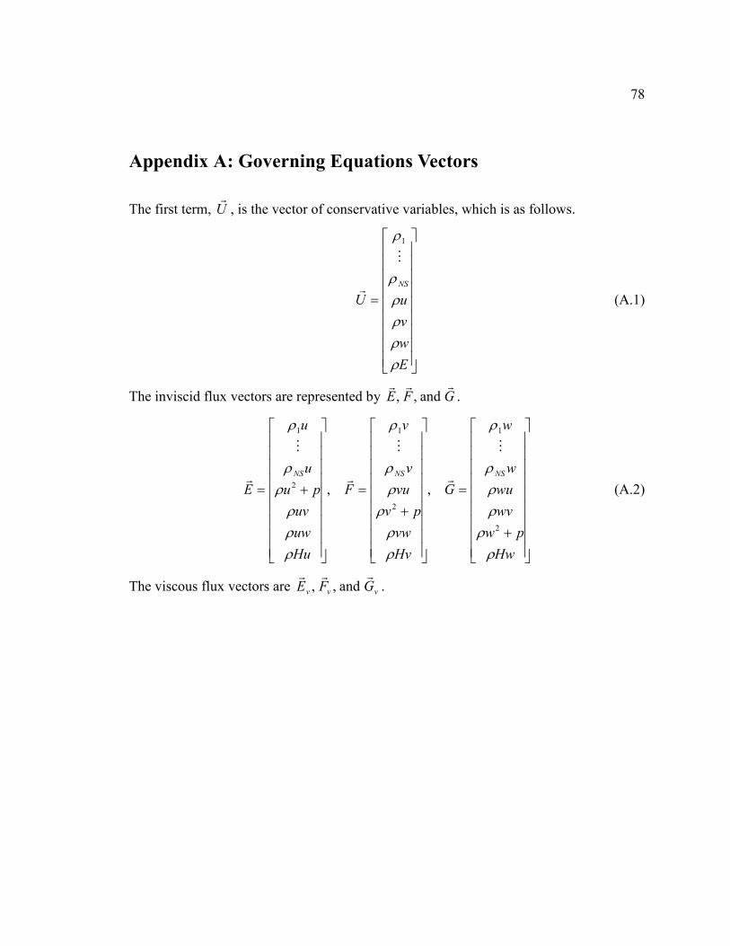
78

Appendix A: Governing Equations Vectors

The first term, Ur, is the vector of conservative variables, which is as follows.

=

E

w

v

uU

NS

ρρρρρ

ρM

r

1

(A.1)

The inviscid flux vectors are represented by GFErrr

and,, .

+

=

+

=

+=

Hw

pw

wv

wu

w

w

G

Hv

vw

pv

vu

v

v

F

Hu

uw

uv

pu

u

u

E

NSNSNS

ρρ

ρρρ

ρ

ρρ

ρρρ

ρ

ρρρ

ρρ

ρ

2

1

2

1

2

1

,,

M

r

M

r

M

r (A.2)

The viscous flux vectors are vvv GFErrr

and,, .

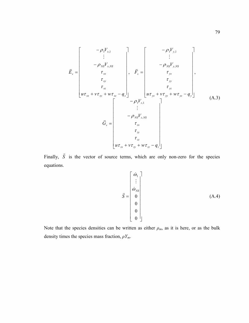
79

−++

−

−

=

−++

−

−

=

−++

−

−

=

zzzzyzx

zz

zy

zx

NSzNS

z

v

yyzyyyx

yz

yy

yx

NSyNS

y

v

xxzxyxx

xz

xy

xx

NSxNS

x

v

qwvu

V

V

G

qwvu

V

V

F

qwvu

V

V

E

ττττττ

ρ

ρτττ

τττ

ρ

ρ

ττττττ

ρ

ρ

,

1,1

,

1,1

,

1,1

,,

M

r

M

r

M

r

(A.3)

Finally, Sr is the vector of source terms, which are only non-zero for the species

equations.

=

0

0

0

0

1

NS

S

ω

ω

&

M

&

r (A.4)

Note that the species densities can be written as either ρm, as it is here, or as the bulk

density times the species mass fraction, ρYm.

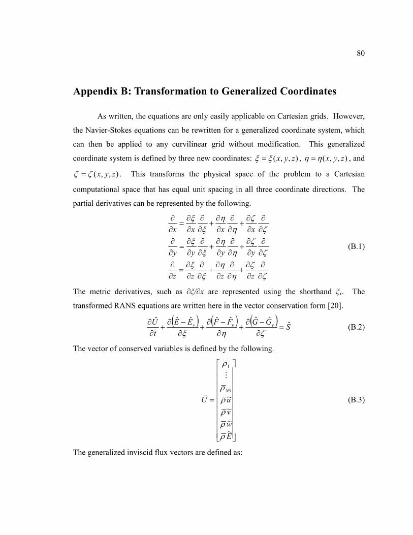
80

Appendix B: Transformation to Generalized Coordinates

As written, the equations are only easily applicable on Cartesian grids. However,

the Navier-Stokes equations can be rewritten for a generalized coordinate system, which

can then be applied to any curvilinear grid without modification. This generalized

coordinate system is defined by three new coordinates: ),,( zyxξξ = , ),,( zyxηη = , and

),,( zyxζζ = . This transforms the physical space of the problem to a Cartesian

computational space that has equal unit spacing in all three coordinate directions. The

partial derivatives can be represented by the following.

ζζ

ηη

ξξ

ζζ

ηη

ξξ

ζζ

ηη

ξξ

∂∂

∂∂

+∂∂

∂∂

+∂∂

∂∂

=∂∂

∂∂

∂∂

+∂∂

∂∂

+∂∂

∂∂

=∂∂

∂∂

∂∂

+∂∂

∂∂

+∂∂

∂∂

=∂∂

zzzz

yyyy

xxxx

(B.1)

The metric derivatives, such as ∂ξ/∂x are represented using the shorthand ξx. The

transformed RANS equations are written here in the vector conservation form [20].

( ) ( ) ( )

SGGFFEE

t

U vvv ˆˆˆˆˆˆˆˆ

=∂−∂

+∂−∂

+∂−∂

+∂∂

ζηξ (B.2)

The vector of conserved variables is defined by the following.

=

E

w

v

uU

NS

~

~

~

~ˆ

1

ρρρρρ

ρM

(B.3)

The generalized inviscid flux vectors are defined as:

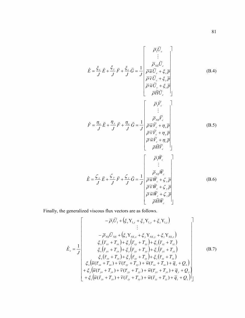
81

+

+

+=++=

c

zc

yc

xc

cNS

c

zyx

UH

pUw

pUv

pUu

U

U

JG

JF

JE

JE

~~

~~

~~

~~

~

~

1ˆ

1

ρξρξρξρ

ρ

ρ

ξξξ

M

rrr (B.4)

+

+

+=++=

c

zc

yc

xc

cNS

c

zyx

VH

pVw

pVv

pVu

V

V

JG

JF

JE

JF

~~

~~

~~

~~

~

~

1ˆ

1

ρηρηρηρ

ρ

ρ

ηηη

M

rrr (B.5)

+

+

+=++=

c

zc

yc

xc

cNS

c

zyx

WH

pWw

pWv

pWu

W

W

JG

JF

JE

JE

~~

~~

~~

~~

~

~

1ˆ

1

ρζρζρζρ

ρ

ρ

ζζζ

M

rrr (B.6)

Finally, the generalized viscous flux vectors are as follows.

( )

( )( ) ( ) ( )( ) ( ) ( )( ) ( ) ( )

( )( )( )

++++++++

++++++++

++++++++++++

+++++

+++++

+++−

+++−

=

zzzzzzxyzyzxzxz

yyyzyzyyyyyxyxy

xxxzxzxyxyxxxxx

zzzzzzyzyyzxzxx

yzyzzyyyyyyxyxx

xzxzzxyxyyxxxxx

zNSzyNSyxNSxNSNS

zzyyxx

v

QqTwTvTu

QqTwTvTu

QqTwTvTu

TTT

TTT

TTT

U

U

JE

)(~)(~)(~)(~)(~)(~)(~)(~)(~

YYY~

YYY~

1ˆ

,,,

,1,1,111

τττξτττξ

τττξτξτξτξτξτξτξτξτξτξξξξρ

ξξξρM

(B.7)

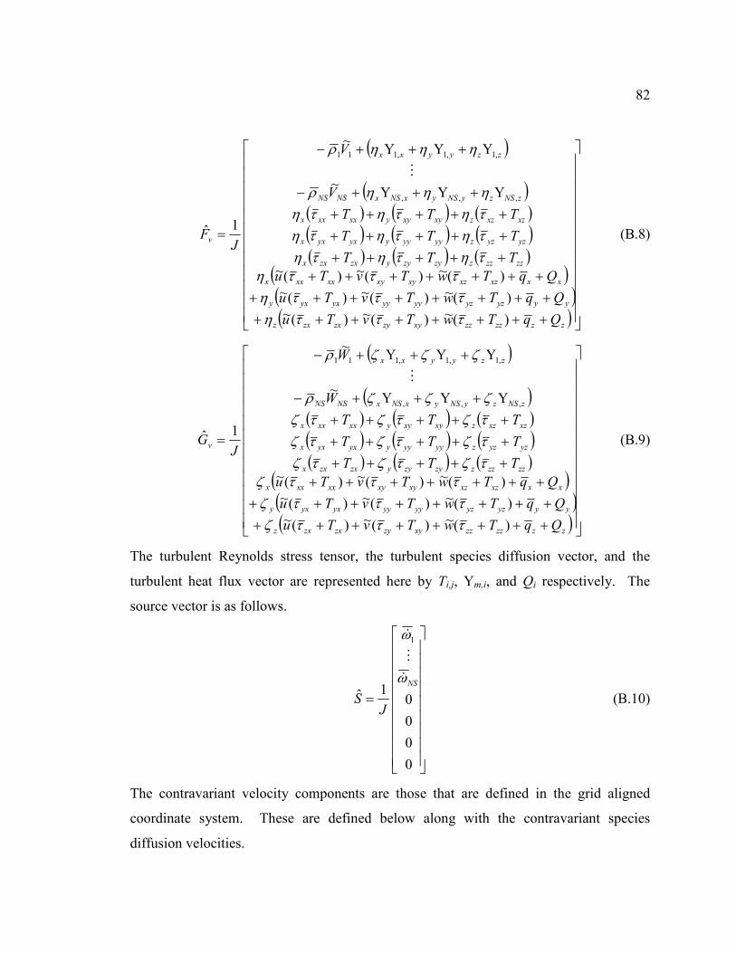
82

( )

( )( ) ( ) ( )( ) ( ) ( )( ) ( ) ( )

( )( )( )

++++++++

++++++++

++++++++++++

+++++

+++++

+++−

+++−

=

zzzzzzxyzyzxzxz

yyyzyzyyyyyxyxy

xxxzxzxyxyxxxxx

zzzzzzyzyyzxzxx

yzyzzyyyyyyxyxx

xzxzzxyxyyxxxxx

zNSzyNSyxNSxNSNS

zzyyxx

v

QqTwTvTu

QqTwTvTu

QqTwTvTu

TTT

TTT

TTT

V

V

JF

)(~)(~)(~)(~)(~)(~)(~)(~)(~

YYY~

YYY~

1ˆ

,,,

,1,1,111

τττητττη

τττητητητητητητητητητηηηηρ

ηηηρM

(B.8)

( )

( )( ) ( ) ( )( ) ( ) ( )( ) ( ) ( )

( )( )( )

++++++++

++++++++

++++++++++++

+++++

+++++

+++−

+++−

=

zzzzzzxyzyzxzxz

yyyzyzyyyyyxyxy

xxxzxzxyxyxxxxx

zzzzzzyzyyzxzxx

yzyzzyyyyyyxyxx

xzxzzxyxyyxxxxx

zNSzyNSyxNSxNSNS

zzyyxx

v

QqTwTvTu

QqTwTvTu

QqTwTvTu

TTT

TTT

TTT

W

W

JG

)(~)(~)(~)(~)(~)(~)(~)(~)(~

YYY~

YYY~

1ˆ

,,,

,1,1,111

τττζτττζ

τττζτζτζτζτζτζτζτζτζτζζζζρ

ζζζρM

(B.9)

The turbulent Reynolds stress tensor, the turbulent species diffusion vector, and the

turbulent heat flux vector are represented here by Ti,j, Ym,i, and Qi respectively. The

source vector is as follows.

=

0

0

0

01ˆ

1

NS

JS

ω

ω

&

M

&

(B.10)

The contravariant velocity components are those that are defined in the grid aligned

coordinate system. These are defined below along with the contravariant species

diffusion velocities.

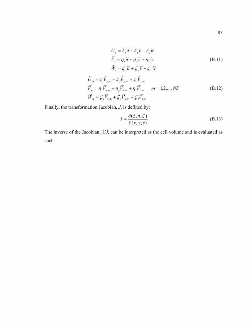
83

wvuW

wvuV

wvuU

zyxc

zyxc

zyxc

~~~~

~~~~

~~~~

ζζζ

ηηη

ξξξ

++=

++=

++=

(B.11)

NSm

VVVW

VVVV

VVVU

mzzmyymxxm

mzzmyymxxm

mzzmyymxxm

,...,2,1

~~~~

~~~~

~~~~

,,,

,,,

,,,

=

++=

++=

++=

ζζζ

ηηη

ξξξ

(B.12)

Finally, the transformation Jacobian, J, is defined by:

),,(

),,(

zyxJ

∂∂

=ζηξ (B.13)

The inverse of the Jacobian, 1/J, can be interpreted as the cell volume and is evaluated as

such.

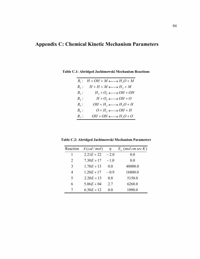
84

Appendix C: Chemical Kinetic Mechanism Parameters

Table C.1: Abridged Jachimowski Mechanism Reactions

OOH

HOH

HOH

OOH

OHOH

MH

MOH

OHOH

HO

HOH

OH

OH

MHH

MOHH

R

R

R

R

R

R

R

+

+

+

+

+

+

+

→←

→←

→←

→←

→←

→←

→←

+

+

+

+

+

++

++

2

2

2

2

2

2

2

22

7

6

5

4

3

2

1

:

:

:

:

:

:

:

Table C.2: Abridged Jachimowski Mechanism Parameters

0.10900.01230.67

0.62687.20406.56

0.51500.01320.25

0.168009.01720.14

0.480000.01370.13

0.00.11730.72

0.00.22221.21

)()/(Reaction

+

+

+

−+

+

−+

−+

E

E

E

E

E

E

E

KseccmmolEmolcalA aη

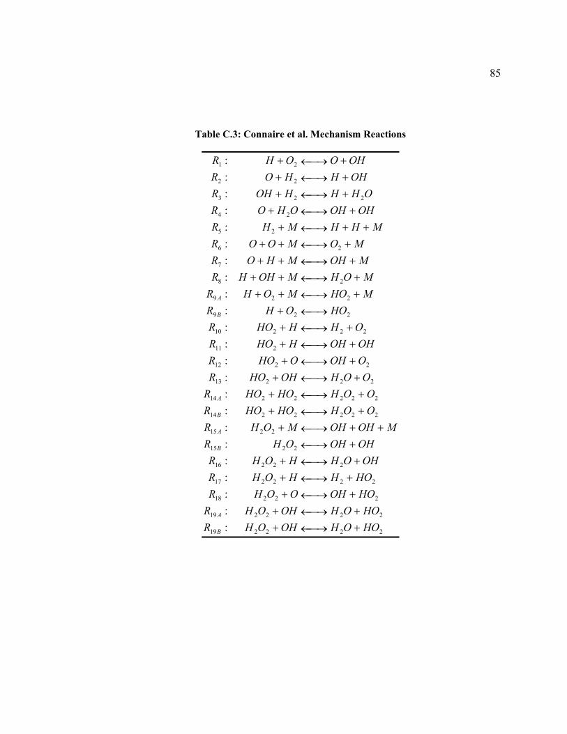
85

Table C.3: Connaire et al. Mechanism Reactions

22

22

2

22

2

222

222

22

2

22

2

2

2

2

2

22

22

22

22

22

22

22

22

22

2

2

2

2

2

2

2

2

2

2

2

19

19

18

17

16

15

15

14

14

13

12

11

10

9

9

8

7

6

5

4

3

2

1

:

:

:

:

:

:

:

:

:

:

:

:

:

:

:

:

:

:

:

:

:

:

:

HOOH

HOOH

HOOH

HOH

OHOH

OHOH

MOHOH

OOH

OOH

OOH

OOH

OHOH

OH

HO

MHO

MOH

MOH

MO

MHH

OHOH

OHH

OHH

OHO

OHOH

OHOH

OOH

HOH

HOH

OH

MOH

HOHO

HOHO

OHHO

OHO

HHO

HHO

OH

MOH

MOHH

MHO

MOO

MH

OHO

HOH

HO

OH

R

R

R

R

R

R

R

R

R

R

R

R

R

R

R

R

R

R

R

R

R

R

R

B

A

B

A

B

A

B

A

+

+

+

+

+

+

++

+

+

+

+

+

+

+

+

+

+

++

+

+

+

+

→←

→←

→←

→←

→←

→←

→←

→←

→←

→←

→←

→←

→←

→←

→←

→←

→←

→←

→←

→←

→←

→←

→←

+

+

+

+

+

+

+

+

+

+

+

+

+

++

++

++

++

+

+

+

+

+

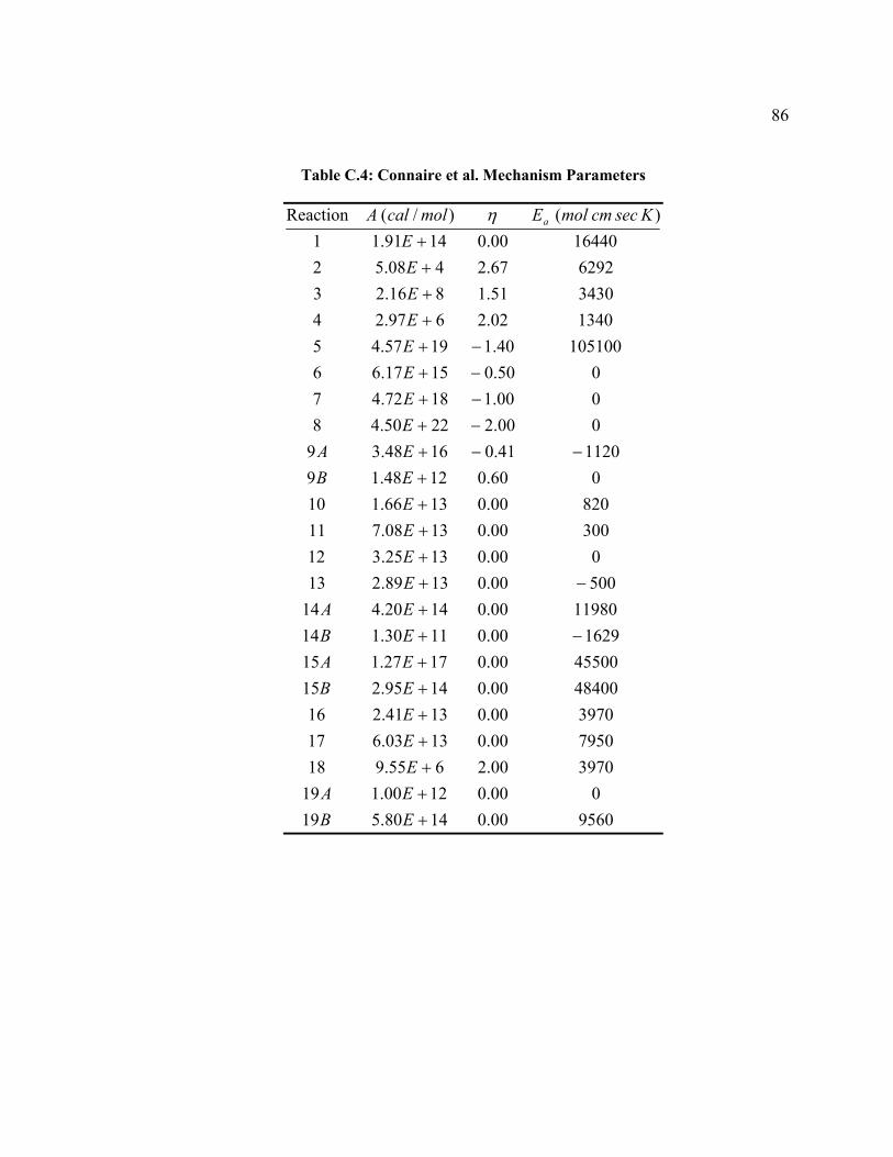
86

Table C.4: Connaire et al. Mechanism Parameters

956000.01480.519

000.01200.119

397000.2655.918

795000.01303.617

397000.01341.216

4840000.01495.215

4550000.01727.115

162900.01130.114

1198000.01420.414

50000.01389.213

000.01325.312

30000.01308.711

82000.01366.110

060.01248.19

112041.01648.39

000.22250.48

000.11872.47

050.01517.66

10510040.11957.45

134002.2697.24

343051.1816.23

629267.2408.52

1644000.01491.11

)()/(Reaction

+

+

+

+

+

+

+

−+

+

−+

+

+

+

+

−−+

−+

−+

−+

−+

+

+

+

+

EB

EA

E

E

E

EB

EA

EB

EA

E

E

E

E

EB

EA

E

E

E

E

E

E

E

E

KseccmmolEmolcalA aη

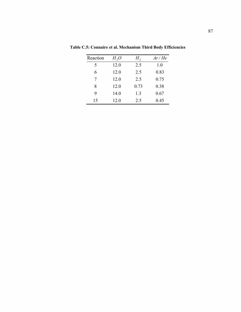
87

Table C.5: Connaire et al. Mechanism Third Body Efficiencies

45.05.20.1215

67.03.10.149

38.073.00.128

75.05.20.127

83.05.20.126

0.15.20.125

/Reaction 22 HeArHOH

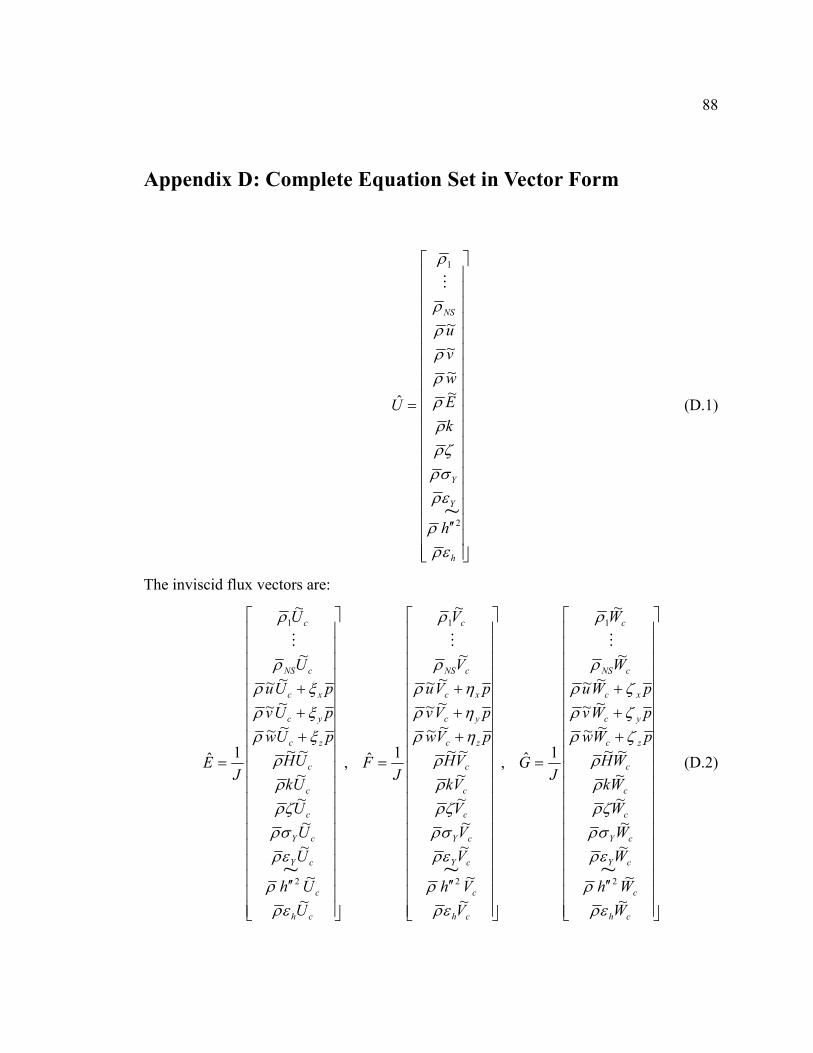
88

Appendix D: Complete Equation Set in Vector Form

′′

=

h

Y

Y

NS

h

k

E

w

v

u

U

ερρ

ερσρζρ

ρρρρρρ

ρ

~2

1

~

~

~

~

ˆ

M

(D.1)

The inviscid flux vectors are:

′′

+

+

+

=

ch

c

cY

cY

c

c

c

zc

yc

xc

cNS

c

U

Uh

U

U

U

Uk

UH

pUw

pUv

pUu

U

U

JE

~

~

~

~

~

~

~~

~~

~~

~~

~

~

1ˆ

~2

1

ερρ

ερσρζρ

ρρ

ξρξρξρ

ρ

ρM

,

′′

+

+

+

=

ch

c

cY

cY

c

c

c

zc

yc

xc

cNS

c

V

Vh

V

V

V

Vk

VH

pVw

pVv

pVu

V

V

JF

~

~

~

~

~

~

~~

~~

~~

~~

~

~

1ˆ

~2

1

ερρ

ερσρζρ

ρρ

ηρηρηρ

ρ

ρM

,

′′

+

+

+

=

ch

c

cY

cY

c

c

c

zc

yc

xc

cNS

c

W

Wh

W

W

W

Wk

WH

pWw

pWv

pWu

W

W

JG

~

~

~

~

~

~

~~

~~

~~

~~

~

~

1ˆ

~2

1

ερρ

ερσρζρ

ρρ

ζρζρζρ

ρ

ρM

(D.2)

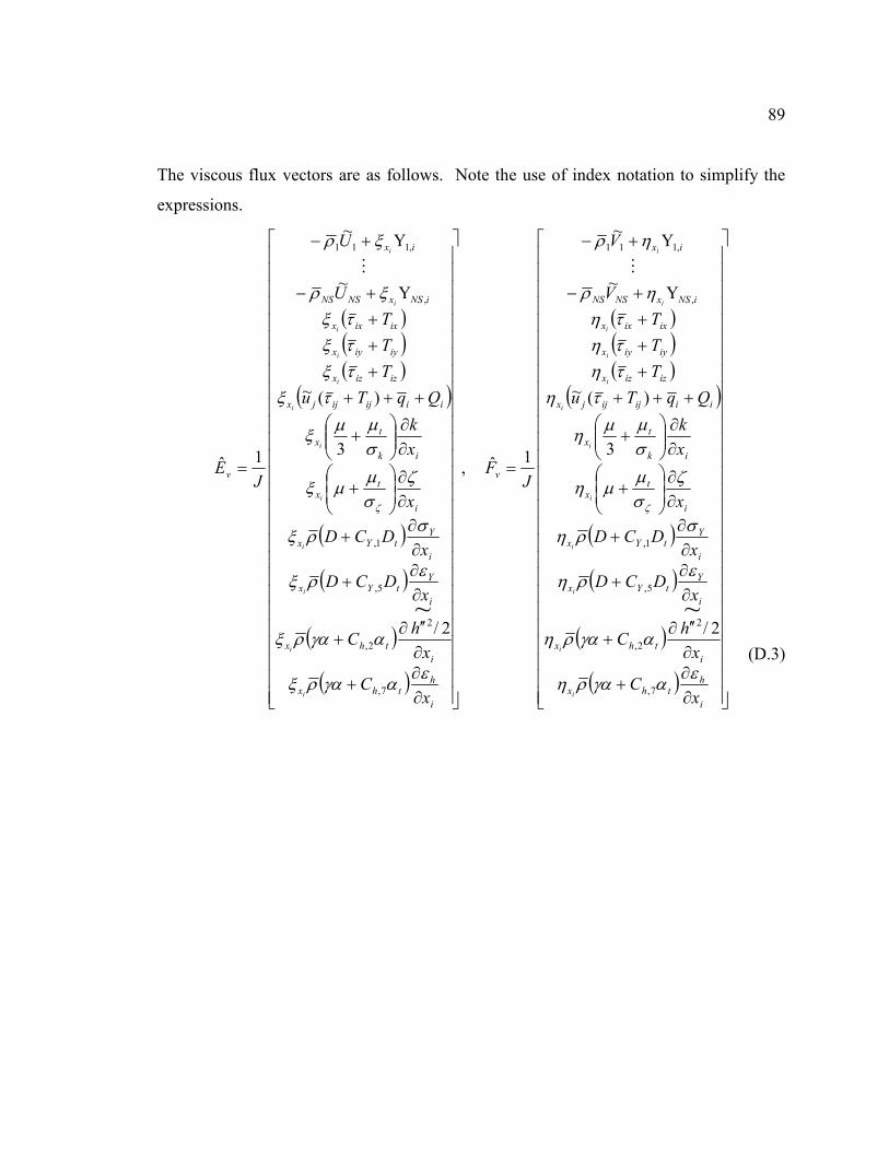
89

The viscous flux vectors are as follows. Note the use of index notation to simplify the

expressions.

( )( )( )

( )

( )

( )

( )

( )

,

2/

3

)(~

Y~

Y~

1ˆ

7,

2

2,

5,

1,

,

,111

~

∂∂

+

∂

′′∂+

∂∂

+

∂∂

+

∂∂

+

∂∂

+

+++

+

+

+

+−

+−

=

i

hthx

i

thx

i

YtYx

i

YtYx

i

tx

ik

tx

iiijijjx

izizx

iyiyx

ixixx

iNSxNSNS

ix

v

xC

x

hC

xDCD

xDCD

x

x

k

QqTu

T

T

T

U

U

JE

i

i

i

i

i

i

i

i

i

i

i

i

εαγαρξ

αγαρξ

ερξ

σρξ

ζσµ

µξ

σµµ

ξ

τξτξτξτξ

ξρ

ξρ

ζ

M

( )( )( )

( )

( )

( )

( )

( )

∂∂

+

∂

′′∂+

∂∂

+

∂∂

+

∂∂

+

∂∂

+

+++

+

+

+

+−

+−

=

i

hthx

i

thx

i

YtYx

i

YtYx

i

tx

ik

tx

iiijijjx

izizx

iyiyx

ixixx

iNSxNSNS

ix

v

xC

x

hC

xDCD

xDCD

x

x

k

QqTu

T

T

T

V

V

JF

i

i

i

i

i

i

i

i

i

i

i

i

εαγαρη

αγαρη

ερη

σρη

ζσµ

µη

σµµ

η

τητητητη

ηρ

ηρ

ζ

7,

2

2,

5,

1,

,

,111

2/

3

)(~

Y~

Y~

1ˆ

~

M

(D.3)

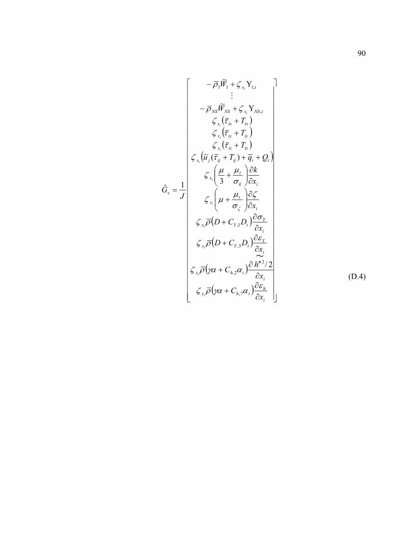
90

( )( )( )

( )

( )

( )

( )

( )

∂∂

+

∂

′′∂+

∂∂

+

∂∂

+

∂∂

+

∂∂

+

+++

+

+

+

+−

+−

=

i

hthx

i

thx

i

YtYx

i

YtYx

i

tx

ik

tx

iiijijjx

izizx

iyiyx

ixixx

iNSxNSNS

ix

v

xC

x

hC

xDCD

xDCD

x

x

k

QqTu

T

T

T

W

W

JG

i

i

i

i

i

i

i

i

i

i

i

i

εαγαρζ

αγαρζ

ερζ

σρζ

ζσµ

µζ

σµµ

ζ

τζτζτζτζ

ζρ

ζρ

ζ

7,

2

2,

5,

1,

,

,111

2/

3

)(~

Y~

Y~

1ˆ

~

M

(D.4)

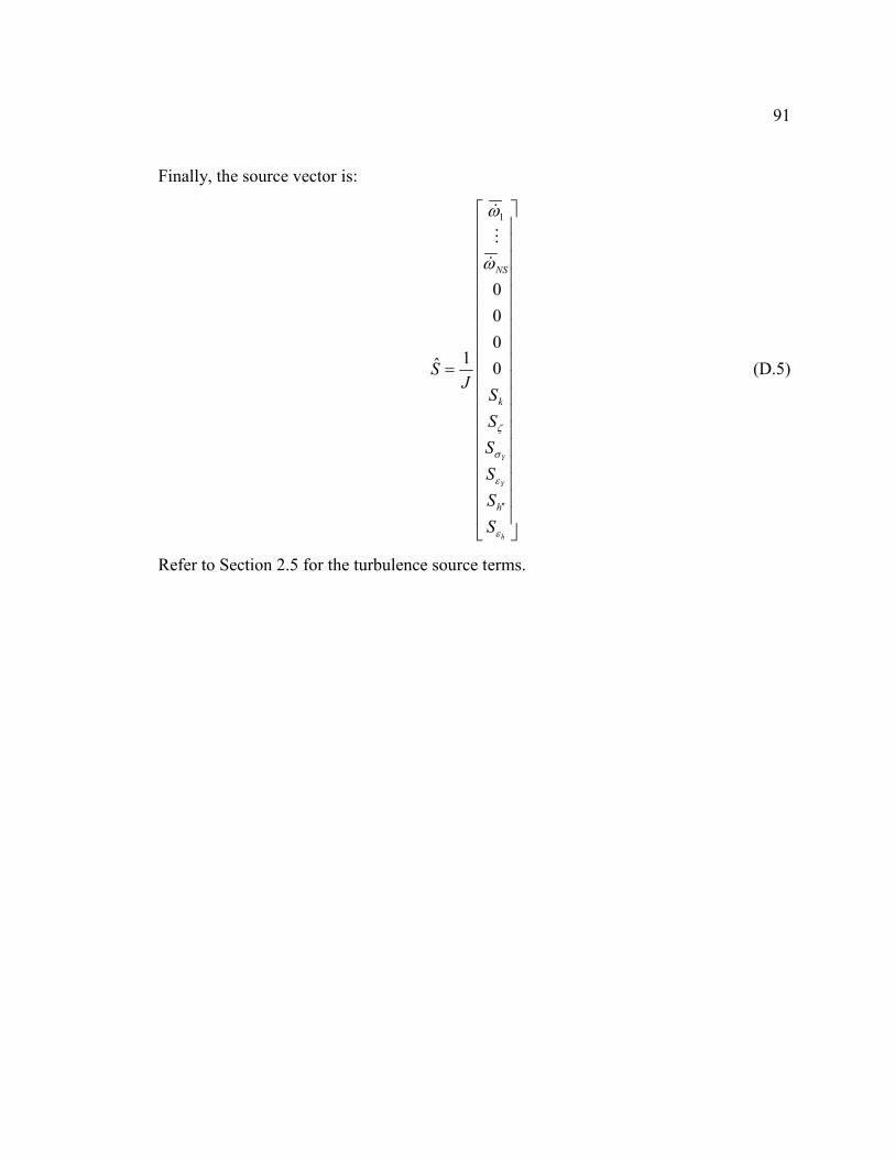
91

Finally, the source vector is:

=

′′

h

Y

Y

S

S

S

S

S

SJ

S

h

k

NS

ε

ε

σ

ζ

ω

ω

0

0

0

0

1ˆ

1

&

M

&

(D.5)

Refer to Section 2.5 for the turbulence source terms.

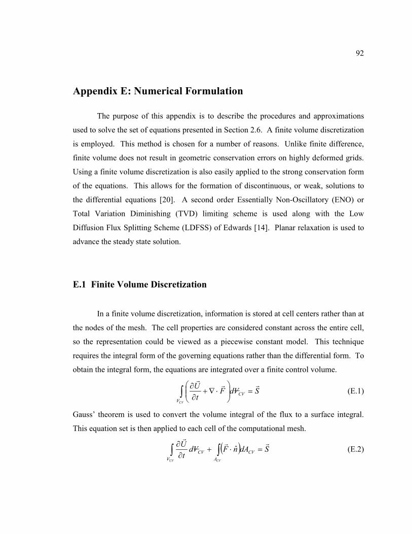
92

Appendix E: Numerical Formulation

The purpose of this appendix is to describe the procedures and approximations

used to solve the set of equations presented in Section 2.6. A finite volume discretization

is employed. This method is chosen for a number of reasons. Unlike finite difference,

finite volume does not result in geometric conservation errors on highly deformed grids.

Using a finite volume discretization is also easily applied to the strong conservation form

of the equations. This allows for the formation of discontinuous, or weak, solutions to

the differential equations [20]. A second order Essentially Non-Oscillatory (ENO) or

Total Variation Diminishing (TVD) limiting scheme is used along with the Low

Diffusion Flux Splitting Scheme (LDFSS) of Edwards [14]. Planar relaxation is used to

advance the steady state solution.

E.1 Finite Volume Discretization

In a finite volume discretization, information is stored at cell centers rather than at

the nodes of the mesh. The cell properties are considered constant across the entire cell,

so the representation could be viewed as a piecewise constant model. This technique

requires the integral form of the governing equations rather than the differential form. To

obtain the integral form, the equations are integrated over a finite control volume.

SVdFt

U

CVV

CV

rrr

=

⋅∇+

∂∂

∫ (E.1)

Gauss’ theorem is used to convert the volume integral of the flux to a surface integral.

This equation set is then applied to each cell of the computational mesh.

( ) SdAnFVdt

U

CVCV A

CV

V

CV

rrr

=⋅+∂∂

∫∫ ˆ (E.2)

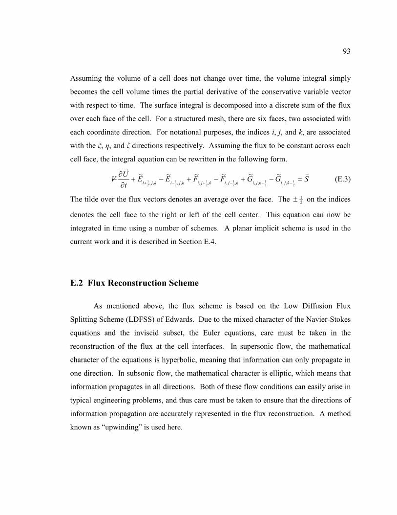
93

Assuming the volume of a cell does not change over time, the volume integral simply

becomes the cell volume times the partial derivative of the conservative variable vector

with respect to time. The surface integral is decomposed into a discrete sum of the flux

over each face of the cell. For a structured mesh, there are six faces, two associated with

each coordinate direction. For notational purposes, the indices i, j, and k, are associated

with the ξ, η, and ζ directions respectively. Assuming the flux to be constant across each

cell face, the integral equation can be rewritten in the following form.

SGGFFEEt

UV

kjikjikjikjikjikji

rr

=−+−+−+∂∂

−+−+−+21

21

21

21

21

21 ,,,,,,,,,,,,

~~~~~~ (E.3)

The tilde over the flux vectors denotes an average over the face. The 21± on the indices

denotes the cell face to the right or left of the cell center. This equation can now be

integrated in time using a number of schemes. A planar implicit scheme is used in the

current work and it is described in Section E.4.

E.2 Flux Reconstruction Scheme

As mentioned above, the flux scheme is based on the Low Diffusion Flux

Splitting Scheme (LDFSS) of Edwards. Due to the mixed character of the Navier-Stokes

equations and the inviscid subset, the Euler equations, care must be taken in the

reconstruction of the flux at the cell interfaces. In supersonic flow, the mathematical

character of the equations is hyperbolic, meaning that information can only propagate in

one direction. In subsonic flow, the mathematical character is elliptic, which means that

information propagates in all directions. Both of these flow conditions can easily arise in

typical engineering problems, and thus care must be taken to ensure that the directions of

information propagation are accurately represented in the flux reconstruction. A method

known as “upwinding” is used here.

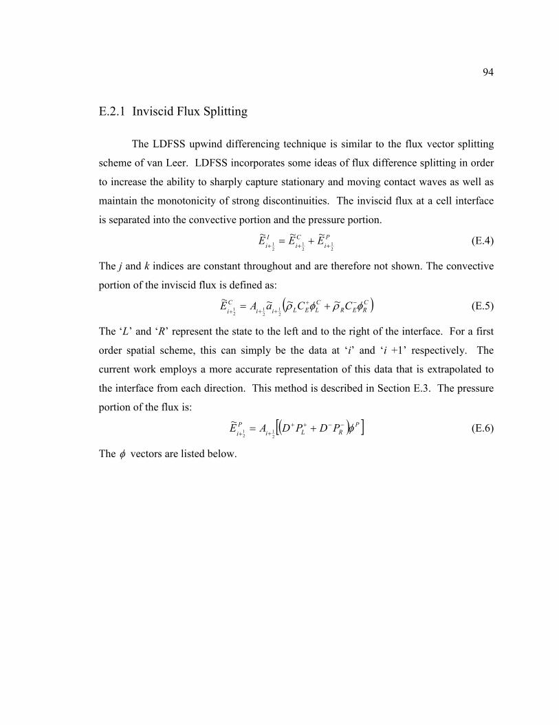
94

E.2.1 Inviscid Flux Splitting

The LDFSS upwind differencing technique is similar to the flux vector splitting

scheme of van Leer. LDFSS incorporates some ideas of flux difference splitting in order

to increase the ability to sharply capture stationary and moving contact waves as well as

maintain the monotonicity of strong discontinuities. The inviscid flux at a cell interface

is separated into the convective portion and the pressure portion.

P

i

C

i

I

iEEE

2

1

2

1

2

1

~~~+++

+= (E.4)

The j and k indices are constant throughout and are therefore not shown. The convective

portion of the inviscid flux is defined as:

( )CRER

C

LELii

C

iCCaAE φρφρ −+

++++= ~~~~

2

1

2

112

(E.5)

The ‘L’ and ‘R’ represent the state to the left and to the right of the interface. For a first

order spatial scheme, this can simply be the data at ‘i’ and ‘i +1’ respectively. The

current work employs a more accurate representation of this data that is extrapolated to

the interface from each direction. This method is described in Section E.3. The pressure

portion of the flux is:

( )[ ]PRLi

P

iPDPDAE φ−−++

+++=

2

112

~ (E.6)

The φ vectors are listed below.

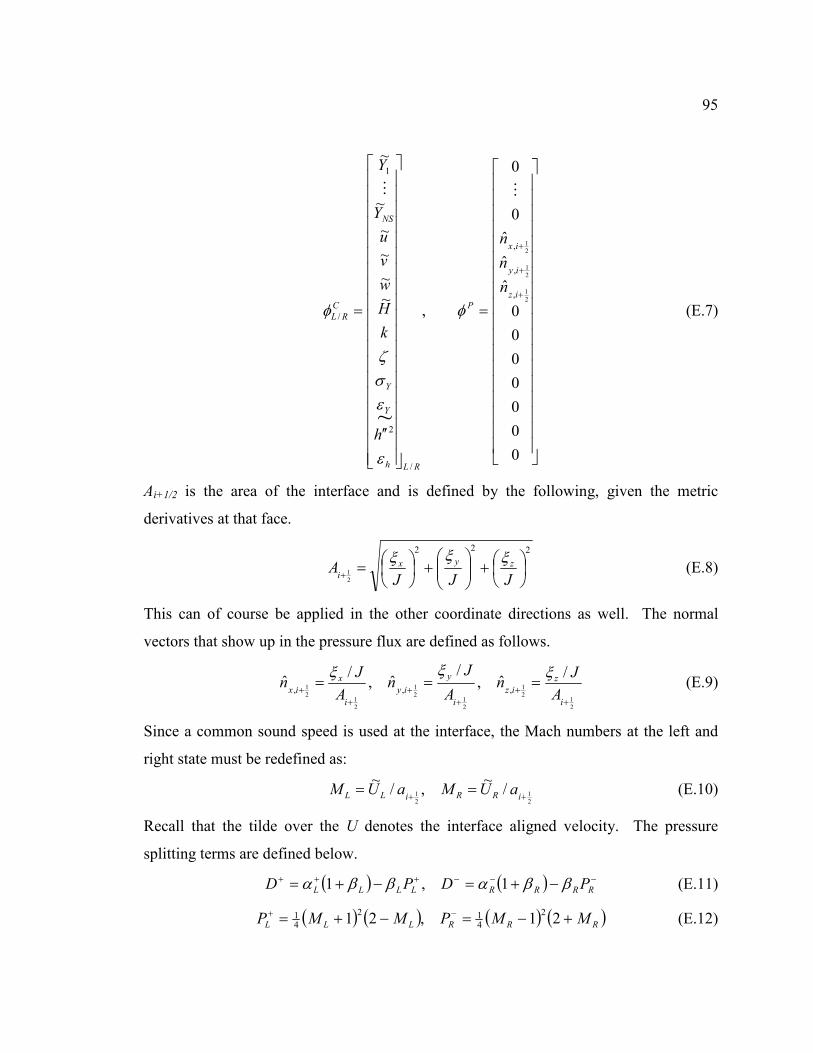
95

=

′′

=+

+

+

0

0

0

0

0

0

0

ˆ

ˆ

ˆ

0

0

,~

~

~

~

~

~

2

1

21

21

,

,

,

/

2

1

/

~

iz

iy

ix

P

RLh

Y

Y

NS

C

RL

n

n

n

h

k

H

w

v

u

Y

Y

MM

φ

ε

εσζ

φ (E.7)

Ai+1/2 is the area of the interface and is defined by the following, given the metric

derivatives at that face.

222

21

+

+

=+ JJJ

A zyx

i

ξξξ (E.8)

This can of course be applied in the other coordinate directions as well. The normal

vectors that show up in the pressure flux are defined as follows.

21

2

1

21

2

1

21

2

1

/ˆ,

/ˆ,

/ˆ

,,,

++

++

++

===i

z

iz

i

y

iy

i

x

ix A

Jn

A

Jn

A

Jn

ξξξ (E.9)

Since a common sound speed is used at the interface, the Mach numbers at the left and

right state must be redefined as:

21

21 /

~,/

~++

==iRRiLL aUMaUM (E.10)

Recall that the tilde over the U denotes the interface aligned velocity. The pressure

splitting terms are defined below.

( ) ( ) −−−+++ −+=−+= RRRRLLLL PDPD ββαββα 1,1 (E.11)

( ) ( ) ( ) ( )RRRLLL MMPMMP +−=−+= −+ 21,212

412

41 (E.12)

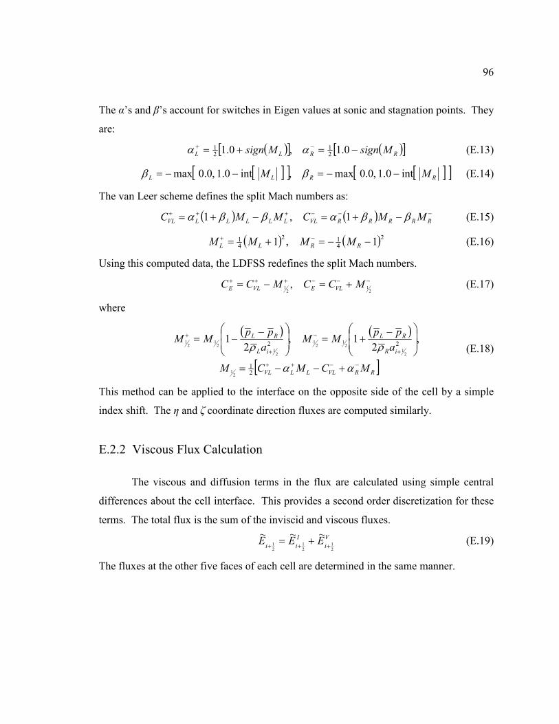
96

The α’s and β’s account for switches in Eigen values at sonic and stagnation points. They

are:

( )[ ] ( )[ ]RRLL MsignMsign −=+= −+ 0.1,0.121

21 αα (E.13)

[ ][ ] [ ][ ]RRLL MM int0.1,0.0max,int0.1,0.0max −−=−−= ββ (E.14)

The van Leer scheme defines the split Mach numbers as:

( ) ( ) −−−+++ −+=−+= RRRRRVLLLLLLVL MMCMMC ββαββα 1,1

(E.15)

( ) ( )2412

41 1,1 −−=+= −+

RRLL MMMM (E.16)

Using this computed data, the LDFSS redefines the split Mach numbers.

−−−+++ +=−=21

21 , MCCMCC VLEVLE (E.17)

where

( ) ( )

[ ]RRVLLLVL

iR

RL

iL

RL

MCMCM

a

ppMM

a

ppMM

−−++

+

−

+

+

+−−=

−+=

−−=

αα

ρρ

21

22

21

21

21

21

21

21

21 ,

21,

21

(E.18)

This method can be applied to the interface on the opposite side of the cell by a simple

index shift. The η and ζ coordinate direction fluxes are computed similarly.

E.2.2 Viscous Flux Calculation

The viscous and diffusion terms in the flux are calculated using simple central

differences about the cell interface. This provides a second order discretization for these

terms. The total flux is the sum of the inviscid and viscous fluxes.

V

i

I

iiEEE

2

1

2

1

2

1

~~~+++

+= (E.19)

The fluxes at the other five faces of each cell are determined in the same manner.

97

E.3 Higher Order Extension

A higher order spatial discretization can be achieved if the conservative or

primitive variables are extrapolated to the cell interfaces rather than assuming that the

properties are constant across the entire cell. A method known as the Monotone Upwind

Scheme for Conservation Laws (MUSCL extrapolation) is used in the current work [20].

Rather than assuming a piecewise constant distribution of properties, the data is assumed

to be piecewise linear or quadratic. The Kappa scheme is based on this idea.

( ) ( )[ ]iiiL uuuurrrr

∆++∆−+= − κκ 114

11 (E.20)

( ) ( )[ ]iiiR uuuurrrr

∆++∆−−= ++ κκ 114

111 (E.21)

iii uuurrr

−=∆ +1 (E.22)

Again, the j and k indices are assumed to be constant, and this method can be applied in

those directions as well. The resulting extrapolation depends on the value chosen for

kappa. A full upwind, full downwind, or a weighted average can result.

As with most high order schemes, some numerical dispersion is induced in

regions with steep gradients or near discontinuities. A method called “slope limiting” is

used to reduce or eliminate these oscillations. By limiting the slopes on either side of the

interface, it can be ensured that no new local maxima or minima develop in the solution.

One class of limiting schemes is called Total Variation Diminishing (TVD) schemes.

This method ensures that the so called total variation of the solution will either decrease

or remain the same. The total variation is:

∑ −= +InterfacesAll

ii uuTVrr

1 (E.23)

The slopes are scaled by a function of the ratio of the adjacent slopes. One such limiting

function is called the Van Albada limiter. The functional form of this limiter is as

follows, where r is the ratio of two adjacent slopes.

2

2

1)(

r

rrr

++

=Ψ (E.24)

98

This is a smooth limiter that lies in the middle of the second order TVD range and is

generally not too compressive or too dissipative. However, it does tend toward the

dissipative extreme as the value of r increases. This limiter also has the property of being

symmetric, which means that the following relation holds.

( ) ( )rrrΨ=Ψ 11 (E.25)

When this is the case, the dependence on kappa vanishes and the final extrapolated

variables are obtained with the following equations.

( )( )12/12

1−

+− −Ψ+= iiiiL uuruu

rrrr (E.26)

( )( )122/312

1++

−++ −Ψ−= iiiiR uuruu

rrrr (E.27)

1

2/3

1

2/1 ,−

−+

+

+− ∆

∆=

∆∆

=i

ii

i

ii

u

ur

u

ur r

r

r

r

(E.28)

Another class of extrapolation methods is called Essentially Non-Oscillatory

(ENO) schemes. When symmetric limiters are applied to the kappa scheme, the data

model is essentially reduced to linear model, losing any ability to produce piecewise

quadratic data. ENO schemes attempt to recover this loss by extending the stencil of the

extrapolation. The main goal of these schemes is to maintain smooth extremes in a

solution. The SONIC-A scheme, which is an ENO extension of the van Leer TVD

limiter is defined by the following set of equations.

2

,2

11

xauu

xauu iiRiiL

∆−=

∆+= ++

rrrr (E.29)

[ ]

+= −+

ii

ii

ii tsss

tsigna ,2max,2

~~

min)(2/12/1

(E.30)

∆

+−∆

+−∆+=

∆

+−∆

+−∆−=

−−−+−−

++−+++

2

21

2

112/12/1

2

12

2

112/12/1

2,

2

2

~

2,

2

2

~

x

uuu

x

uuummdx

ss

x

uuu

x

uuummdx

ss

iiiiiiii

iiiiiiii

(E.31)

x

uus

x

uus ii

iii

i ∆

−=

∆

−= −

−+

+1

2/11

2/1 , (E.32)

99

[ ]2/12/1~,~

−+≡ iii ssmmdt (E.33)

[ ]2/12/1 , −+≡ iii ssmmds (E.34)

Once the variables are extrapolated to the cell interfaces, the fluxes can be

calculated using the methods described in Section E.2.

E.4 Time Integration

The goal of the numerical solver is to advance the solution in time until a steady

state is reached, such that the solution does not change with further advancement. An

implicit method is chosen over an explicit method meaning that the residual is evaluated

at the next time step rather than the current time step. The residual is simply the sum of

the fluxes minus the source vector for each cell.

kji

kjikjikjikjikjikji

kji

R

SGGFFEEt

uV

,,

,,,,,,,,,,,,

,,)

~~~~~~(

2

1

2

1

2

1

2

1

2

1

2

1

r

rr

−≡

−−+−+−−=∂

∂−+−+−+ (E.35)

The time discretization is called the backward Euler scheme, which is as follows.

( ) 011

=+

∆− +

+n

nn

uRt

uuV

rrrr

(E.36)

Consider a system of equations consisting of all equations solved per mesh cell times the

number of mesh cells. The system is denoted by the nonlinear operator )(uRrr. This

system is then linearized as follows.

( ) ( )nnn uRuuu

R

t

V rrrrr

r

−=−

∂∂

+∆

+1 (E.37)

Some simplifications are taken in formulating the system jacobian uRrr

∂∂ / . First,

consider the residual vector to be spatially first order, regardless of the spatial order of the

residual on the right hand side of the equation. Also, the jacobian is formulated based

100

only on the inviscid fluxes. The residual vector for a single mesh cell is a function of the

data in that cell and the six adjacent cells.

( ) ( )( ) ( )( ) ( )1,,1

1,,,,

1

,,

1

1,,,,

1

,,

1

,1,,,

1

,,

1

,1,,,

1

,,

1

,,1,,

1

,,

1

,,1,,

1

,,

,~

,~

,~

,~

,~

,~

21

21

21

21

21

21

++−−

++++

++−−

++++

++−−

++++

+

−+

−+

−=

n

kji

n

kjikji

n

kji

n

kjikji

n

kji

n

kjikji

n

kji

n

kjikji

n

kji

n

kjikji

n

kji

n

kjikji

n

kji

uuGuuG

uuFuuF

uuEuuER

rrrr

rrrr

rrrrr

(E.38)

Differentiating this with respect to the conservative variable vector produces the

following equation for the Euler Implicit form.

( )n

kji

n

kjikji

n

kjikji

n

kjikji

n

kjikji

n

kjikji

n

kjikji

n

kjikji

uRuGuFuE

uDuCuBuA

,,

1

1,,,,

1

,1,,,

1

1,,,,

1

,,,,

1

1,,,,

1

,1,,,

1

,,1,,

rr−=∆+∆+∆+

∆+∆+∆+∆+

+++

++

++−

+−

+−

(E.39)

where A through G are as follows,

kji

kji

kjiu

EA

,,1

,,

,,21

~

−

−

∂

∂−= r (E.40)

kji

kji

kjiu

FB

,1,

,,

,,21

~

−

−

∂

∂−= r (E.41)

1,,

,,

,,21

~

−

−

∂

∂−=

kji

kji

kjiu

GC r (E.42)

t

V

u

G

u

G

u

F

u

F

u

E

u

ED

kji

kji

kji

kji

kji

kji

kji

kji

kji

kji

kji

kji

kji ∆+

∂

∂−

∂

∂+

∂

∂−

∂

∂+

∂

∂−

∂

∂= −+−+−+

,,

,,

,,

,,

,,

,,

,,

,,

,,

,,

,,

,,

,,21

21

21

21

21

21

~~~~~~

rrrrrr (E.43)

1,,

,,

,,21

~

+

+

∂

∂−=

kji

kji

kjiu

GE r (E.44)

kji

kji

kjiu

FF

,1,

,,

,,21

~

+

+

∂

∂−= r (E.45)

kji

kji

kjiu

EG

,,1

,,

,,21

~

+

+

∂

∂−= r (E.46)

With nine chemical species, each of these flux jacobians is a 19 by 19 matrix. Another

simplification used here is to lett the interface fluxes be determined by the Lax-Friedrichs

101

scheme. This allows for the simple calculation of derivatives. The Lax-Friedrichs

scheme is:

( )( )kjikjikjikjikjikjiuuIEEE ,,1,,,,,,1,,2

1,, 2

121

~++++ −++=

rrrrσ (E.47)

Sigma is the maximum Eigen value, or spectral radius of the system. The flux Jacobians

for the Navier-Stokes equations can be found in Hirsch [20]. Two final approximations

include zeroing many of the more complicated entries in the flux Jacobians and assuming

that the flux Jacobians approximately cancel in the D coefficient. This makes the D

matrix diagonal.

While this is sufficient for non-reactive systems, systems with chemical source

terms require further accommodations. The characteristic times for chemical reactions

are significantly smaller than any of those present in the convective or diffusive terms.

Therefore, to solve the system implicitly, the source terms must be linearized in addition

to the inviscid fluxes. This results in an additional term, uSrr

∂∂ / , in the A matrix, and

while the matrix itself may be complicated, the derivation of it is straightforward.

An iterative technique is adopted to approximately solve this linear system. The

method is a combination of two techniques, incomplete lower/upper (ILU) decomposition

and symmetric Gauss-Seidel. On each plane of constant i, ILU is used in the j and k

directions while symmetric Gauss-Seidel iteration is used in the i direction.

The linear system can be written as follows.

nn

nn

n

Ru

Ruu

S

u

R

t

V

rr

rrr

r

r

r

−=∆

−=∆

∂∂

−∂∂

+∆

+

+

1

1

A

(E.48)

The ILU method simplifies the A matrix into lower, upper, and diagonal matrices [37].

( ) nnn Ruu −=∆++=∆ ++ 11 rrUDLA (E.49)

CBA ++=L (E.50)

GFE ++=U (E.51)

D is defined as follows:

1,,1,,,,,1,,1,,,,,1,,1,,,,,, ++++++ −−−= kjikjikjikjikjikjikjikjikjikjikji EDCFDBGDADD (E.52)

102

This is performed in both directions. A is approximated by the ILU scheme as follows.

)()( 1UDDDLA ++= −

ILU (E.53)

Using this approximation, a symmetric Gauss-Seidel technique is used to update the

solution in the i direction with a forward and backward sweep defined as follows.

( ) ( )21

21

,,1,,,,

1

,,,,

+−

−+ ∆−−=∆ n

kji

n

kji

n

kji

n

kji

n

kji uRurrr

LD (E.54)

1

,,1,,,,

1

,,21 +

+++ ∆−∆=∆ n

kji

n

kji

n

kji

n

kji uuurrr

U (E.55)

Once the two sweeps have been performed, the solution is updated.

The time step is determined using the Courant Friedrichs and Lewy (CFL)

condition based on the local maximum Eigen values of the system. Since the only

solution of interest is the steady state solution, the temporal accuracy of the preceding

iterations is not of concern. This allows local time stepping to be used, which increases

convergence rates, but decreases the accuracy of any intermediate solution. The time

step is defined by the following.

( ) ( ) ( )

CFL

aWAaVAaUA

t

V ccckji+++++

=∆

~~~,, ζηξ

(E.56)

The A’s represent average projected areas in the three coordinate directions. The CFL

maybe be specified as high as 5 for the current work.

E.4.1 Alternate Solver (Sequential Solution of Turbulence Equations)

Two different methods were used to solve the turbulence equations. One method

includes the six turbulence equations in the planar ILU scheme. The alternative method

solves the species and conservation equations with the planar ILU scheme and then

solves the turbulence equations sequentially using a three-dimensional ILU method

similar to the one described above. The latter is the method of choice and the overall

result is a much faster computation with solutions that are not noticeably different from

the inclusive solver.