Simulation of Sheet Metal Forming Processes Using a Fully ...

Metals 2018, 8, 991; doi:10.3390/met8120991 www.mdpi.com/journal/metals

Article

Simulation of Sheet Metal Forming Processes Using a

Fully Rheological-Damage Constitutive Model

Coupling and a Specific 3D Remeshing Method

Abel Cherouat 1,*, Houman Borouchaki 1 and Zhang Jie 2

1 Department Recherche Opérationnelle, Statistiques Appliquées, University of Technology of Troyes-

GAMMA3-Team INRIA, 12 rue Marie Curie, 10004 Troyes, France; [email protected] 2 Department of Materials Science and Engineering, Shanghai Jiao Tong University, 1954 Huashan Rd,

Xuhui Qu, Shanghai 200000, China; [email protected]

* Correspondence: [email protected]; Tel.: +33-325-715-674

Received: 17 October 2018; Accepted: 20 November 2018; Published: 26 November 2018

Abstract: Automatic process modeling has become an effective tool in reducing the lead-time and

the cost for designing forming processes. The numerical modeling process is performed on a fully

coupled damage constitutive equations and the advanced 3D adaptive remeshing procedure. Based

on continuum damage mechanics, an isotropic damage model coupled with the Johnson–Cook flow

law is proposed to satisfy the thermodynamic and damage requirements in metals. The Lemaitre

damage potential was chosen to control the damage evolution process and the effective

configuration. These fully coupled constitutive equations have been implemented into a Dynamic

Explicit finite element code Abaqus using user subroutine. On the other hand, an adaptive

remeshing scheme in three dimensions is established to constantly update the deformed mesh to

enable tracking of the large plastic deformations. The quantitative effects of coupled ductile damage

and adaptive remeshing on the sheet metal forming are studied, and qualitative comparison with

some available experimental data are given. As illustrated in the presented examples this overall

strategy ensures a robust and efficient remeshing scheme for finite element simulation of sheet

metal-forming processes.

Keywords: continuum damage mechanics; 3D adaptive remeshing; sheet metal forming

1. Introduction

The commercial finite element software has integrated various material models to describe the

thermal-visco-plastic behaviors of sheet metal in different forming processes (deep-drawing,

hydroforming, incremental forming, blanking). However, when materials are formed by these

processes, they experience large plastic deformations leading to the onset of internal or surface micro-

defects as voids and micro cracks. When micro-defects initiate and grow inside the plastically

deformed metal, the thermo-mechanical fields are deeply modified, leading to significant

modifications in the deformation process. On the other hand, the coalescence of micro-voids defects

during the deformation can lead to the initiation of macro-cracks or damaged zones, inducing

irreversible damage inside the formed part and consequently its loss. Taking into account the damage

defect in sheet metal forming necessitates not only the development of a continuum damage theory,

but also its coupling with the other mechanical fields. This is useful to avoid damage initiation to

obtain a non-damaged work-piece (hot forging, stamping, deep-drawing and hydroforming) and

develop the damage initiation and propagation to simulate the machining processes (orthogonal

cutting, blanking, guillotining).

Metals 2018, 8, 991 2 of 38

During the past decades, constitutive models of ductile damaged materials in the finite

deformation range have received considerable attention. An important point in such

phenomenological constitutive models is the appropriate choice of the physical nature of mechanical

variables realistically describing the damage state of materials. Two main methods exist to predict

the macro-defect in sheet metal forming:

a) The first uncoupled approach aims to calculate the damage (initiation and growth) distribution

without taking into account its effect on the other mechanical fields (elastic, thermal, plastic, and

hardening). This approach is used to predict zones where local failure has taken place inside the

deformed work piece. Generally, this is achieved by post-processing the finite element analysis

for a given time step to calculate the damage distribution using the stress and strain fields [1–3].

b) In the second fully coupled approach, the damage effect is directly introduced into the overall

constitutive equations and affects all the mechanical fields. In this case, the damage field

assumes that the degradation of structure is due to nucleation and growth of micro defects and

their coalescence into macro-cracks. The fully coupled approach has shown their ability to

optimize the process plane, not only to avoid the damage occurrence, but also to enhance the

damage in order to simulate any metal cutting processes [4–6].

Damage mechanics in metal assumes that the degradation of material due to nucleation and

growth of micro defects (voids and cracks), and their coalescence into macro-cracks [1–3]. McClintock

[4] firstly develops the relationship between micro defects and ductile failure. After, three main

approaches based on micro-defects [5] are extensively used to describe the damage mechanics:

fracture mechanics [6], micro-based damage mechanics [7–10], and continuum damage mechanics

(CDM). This somewhat fully coupled approach accounts for the direct interactions between the

plastic flow, including different kinds of hardening, and the ductile damage initiation and growth.

In CDM, the damage is assumed to be one of the internal state variables which relates to material

behavior induced by the irreversible deterioration of microstructure. The function of damage variable

works with effective stress. Kachanov [11] is the pioneer to characterized ductile damage by a scalar

to define the effective stress. Without a clear physical meaning for damage, he introduced a scalar

internal variable to model the creep failure of metal under uniaxial loads. A physical significance for

the damage variable was given later by Rabotnov [12] who proposed the reduction of the cross

sectional area due to micro-cracks as a suitable measure of the state of internal damage.

Lemaitre and Chaboche developed the continuum damage mechanic for ductile damage later

[13]. The constitutive equations of damage variables are derived from specific damage potentials by

using the effective state variables. These are defined from the classical state variables using one of the

three following hypotheses: strain equivalence, stress equivalence or energy equivalence. The

coupled constitutive equations of the damaged domain are generally deduced from the same state

and dissipation potentials in which the state variable are replaced by the effective state variables [13–

16].

In recent years, sets of constitutive equations for elasticity, plasticity and thermo-visco-plasticity

coupled with ductile damage are given [15]. The works of Bouchard [17], Brünig [18], and Wang [19]

summarized and compared various damage models.

The Johnson–Cook (JC) hardening model is the most attractive among well-known visco-plastic

strain flow. This model takes into account both kinematic strengthening and adiabatic heating of the

material undergoing strains and can describe the dynamic behavior of materials, which works in

different thermal environments. For these advantages, the JC model has been modified in parameters

and various forms to fit the different material behaviors. Peirs [20] used the advanced experiment

method and finite element simulation tools to verify the material parameters in JC model, especially

the strain rate hardening and thermal softening parameters. Through enhancing the thermal

softening effects, the simulation results using corrected parameters agreed with the experiments and

some strain localization phenomena happened. Calamaz [21] directly changed the JC model to the

form of TANH model. A new term, which is controlled by temperature, was added to simulate the

serrated chips formation in orthogonal cutting process. On the other hand, Zerilli and Armstrong

proposed dislocation-mechanics-based constitutive relations for different crystalline structures, in

Metals 2018, 8, 991 3 of 38

which the effects of strain hardening, strain rate hardening, and thermal softening based on the

thermal activation analysis were incorporated into constitutive relations [22–24]. Holmquist et al. [25]

and Hor et al. and [26] propose a comparison of the models to be made independent of the material

constants and procedure for which constants can be determined for different constitutive models

using the same test data base.

In these models, the damage generates and evolves during tensile, shearing and cutting process

had never introduced. This point is not identical to the practical situation. Actually, the stiffness of

the material is deteriorating until to losing the abilities of loading which is following with the

evolution of damage. Johnson and Cook [27] have given out a threshold, which is a function of stress

state (stress triaxiality) for equivalent plastic strain. The damage generates when equivalent plastic

strain reaches to this threshold. The limitation of this damage model is that, it can only predict the

onset of the damage and the material stiffness will reduce to zero directly without any evolution

process. Some phenomena (like strain localization) are hard to obtain and it will also lead the

instability into the simulation system. Therefore, it is necessary to integrate a constitutive damage

evolution into the JC model. Based on this aspect, a constitutive equation which couple fully the

ductile damage into JC isotropic hardening model, is developed. These fully coupled constitutive

equations have been implemented into a Dynamic Explicit finite element code (Abaqus/Explicit)

using user subroutine. The local integration of the plastic-damage constitutive equations is

performed using an asymptotic implicit scheme applied to solve the nonlinear local equations.

Numerical errors are intrinsic in Finite Element Analysis (FEA) of sheet metal forming processes

and possess additional difficulties related to the large inelastic deformations with damage imply a

severe distortion of the computational domain [28,29]. In fact, the deformed domain undergoes

geometrical variation (large displacements and rotations) and are characterized by inhomogeneous

spatial distribution of thermo-mechanical fields with evolving localized zones (stress, plastic strain,

damage, temperature, etc.). In fact, the time and space discretization of the continuous differential

equations governing the physical equilibrium events lead inevitably to numerical errors. In this case,

frequent remeshing of the deformed domain during computation is necessary to obtain an accurate

solution and complete the computation until the termination of the numerical simulation process.

Accordingly, several remeshing have to be performed during the simulation in order to preserve the

reliability of the obtained results by minimizing errors generated by either the geometrical

transformations or the heterogeneous thermo-mechanical fields.

To decide when the remeshing is required during the analysis, some appropriate criteria are

needed and should be automatically executed during the FEA. These are generally based on a priori

and a posteriori error estimators. The main goal of any error estimator is the evaluation of the

absolute global error as an addition of the estimated local error for each element. For metal forming,

the error criteria is classified into three classes:

(1) Geometrical: estimation of the element distortion due to the large transformation of the domain.

Distortion criteria are based on the large variation of the geometry of finite elements with respect

to their reference state.

(2) Curvature: estimation of the element size needed to avoid inter-penetration between the

deformed domain and complex tools. This geometric estimator is based on the curvature of the

tools angles inside the contact zones.

(3) Physical: adaptation of the element size to the local or global variation of some physical fields as

temperature, displacement gradient, stress, plastic strain etc.

Accordingly, the damage growth induces a decrease in the stress-like variables generated by a

decrease in physical properties of the material. When all Gauss points within a given finite element

are fully damaged, the corresponding stiffness matrix is zero. Consequently, this element has no more

contribution in the global tangent stiffness matrix and should be removed. Accordingly, there is

problem for elements lying in boundaries of the deformed domain need special attention when this

boundary is concerned with the contact zone between different domains (tools and deformable parts).

The best way to treat the fully damaged elements consists in remeshing the domain after dropping

the fully damaged elements and smoothing the newly created boundaries of the deformed part.

Metals 2018, 8, 991 4 of 38

In this work the damage potential, introduced by Lemaitre [13], is used and coupled into an

elasto-visco-plastic material model through defining the effective stress and plastic strain like a

Johnson–Cook formulation [27]. 3D adaptive remeshing scheme using linear tetrahedral finite

element is developed in order to simulate the large plastic deformations and crack propagation after

damage occurring [28,29]. This scheme is established to simulate to predict when and where ductile

damage zones may take place inside the deformed part during tensile, compressive, and shearing

tests. The localization phenomenon of damage was illustrated clearly. The formation of the cracks

and its propagation to the final fracture of the specimen are also illustrated. Four various sheet metal

forming processes are proposed to prove that the numerical methodology is an advanced and a

reliable tool to simulate various metal forming processes in order to avoid damage in incremental

forming, deep drawing, and multi-point drawing or to enhance damage in order to simulate some

sheet metal cutting operations.

2. Methods and Constitutive Model

2.1. Visco-Elastoplastic Model Fully Coupled to Isotropic Ductile Damage

This section provides a brief description of the major conception for coupling the ductile damage

into the material elasto-visco-plastic behavior. The ductile damage is presented in the framework of

irreversible processes with state variables. An isotropic ductile damage variable D (0 < D < 1) is

measured in a macroscopic scale way through the surface density of intersection of micro-cracks and

micro-cavities at a representative finite elementary volume. In order to perform the effect of this

damage variable on the mechanical behavior, the effective state variables are introduced [11–16].

To another consideration, the damage caused by the micro-cracks and micro-cavities has a

different evolution processes in tensile and compressive load conditions. In one aspect, the micro-

cracks are opened in the tensile state and the module of elasticity reduces gradually until to zero. In

another aspect, the micro-cracks are closed in compressive state and the module of elasticity could

be able to restore to their initial values before the damage accumulates. This recovery effect of

physical properties after closure of micro-cracks is called the quasi-unilateral effect [30–37]. It

demands that the definition of effective state variable σ, ε should be in the unilateral condition.

According to the theory of energy equivalence, we define the effective variables, which consider

the isotropic ductile damage into state variables [38–42] as follows:

σσ

1

D, 1

e eε ε D ,

Hσ σ 1S and H

1σ = trσ

3 (1)

where eε is the small elastic strain tensor representing the elastic flow associated with the Cauchy

stress tensor σ , H,σS are the deviatoric and hydrostatic Cauchy stresses respectively and D is the

ductile damage associated with the potential Y.

The damaged elastoplastic behavior is described in the framework of the thermodynamics of

irreversible processes with state variables. The Helmholtz free energy in which elasticity and

plasticity are uncoupled gives the law of elasticity coupled with damage. Following the 2nd principle

of thermodynamics, non-negativity of the mechanical dissipation, the stress like variables ( σ ,Y ) are

derived from the state potential taken as the classical free energy eΨ ε , D in deformation space

[15,16], as follows:

22

2

22

1 2 : :

1 2: : (1 ) 3( )

2 2 ( ) 3

e e

e e

e e H

μ λ 1 1 ε 1 ε

σ σε ε ν 1 2ν

1 σ

JY

E D J

D I D

(2)

where e eλ ,μ are the classical Lame's constants which are a function of Young modulus E and

Poison’s coefficient ν .

Metals 2018, 8, 991 5 of 38

In order to couple the damage behavior, a single appropriate dissipation potential ( )σ,Y,DF

is defined to govern the evolution law for internal variables in the stress space [39–42]:

2pp

p

0

10

)1

p

pα 1

β

σε

σ, ε , ,γ 1

α 1 γ

Y

Y

JD R

DF Y D

Y YY, D

D

f , ,

=f + F

F(

(3)

The parameters (α, β and γ and Y0) are used to control the evolution of damage potential, pεR

is the JC isotropic yield stress in various visco-plastic flow and 2

3

2σ :S SJ is the second invariant

of the deviatoric Cauchy stress S .

For the case of time independent plasticity, the plastic strain rate tensor p

ε and the rate damage

D are obtained from the stationarity conditions as in which the plastic multiplier is deduced from

the consistency condition [13]:

p

2

0

3

2 1

(1 )

p

α

β

λε λ

σ σ

1λ λ

γY

f S

JD

Y YFD

Y D

(4)

where

p pp 2ε ε :ε

3 (5)

is the effective plastic strain rate.

Failure is assumed to initiate when the damage at a material point reaches the critical damage

value Dc. When this happens, the stiffness of the failed element is significantly reduced and

consequently incapable of carrying any load. The value of Dc for any material must be acquired

through experimental tests. Assuming a fully isotropic material behavior, the plastic multiplier λ

is obtained by the consistency condition p p= = 0f f associated with the loading–unloading

condition [13–15]. It is a strictly positive scalar, which plays the role of Lagrange multiplier for

dissipative phenomena:

2( )e

p

1 1λ 3μ 1 : ε

σD S

H J (6)

The non-symmetric fourth order tangent elastoplastic operator TL defining the stress rate

σ : εT

L is defined as [28,29,36,40]:

α

0e e e e1β+

2p 2 2 2p

1 1=2μ 1 3μ Ä3μ 3μ Ä

γσ σ σ1T

D Y YS S SL D S

H J J JH D

(7)

where pH is the tangent plastic hardening module given by:

Metals 2018, 8, 991 6 of 38

3

2

2 ( ) 13

12 1β

α

0e p

σ δμ

γ δε

Y YJ RH

p

DD

(8)

In this paper, the thermal effects are ignored [30–40] and the visco-plastic hardening yield stress

is written as:

1p p

0

εε ε ln

ε

n

R A B C

(9)

Where pε is the equivalent plastic strain, ε is the equivalent plastic strain rate. The initial strain

rate 0ε is determined by experimental conditions. The parameters A, B and n represent the isotropic

hardening evolution and C represent the material viscosity. The fully isotropic rate formulation

assumes the small strain hypothesis in sheet forming processes where relative slow speeds and inertia

effect can be neglected and dynamic phenomena not occur during the process.

For the constitutive equations, this hypothesis is justified by the fact that the applied load

increments are still very small during remeshing procedure of sheet metal forming. Accordingly, the

total strain rate tensor ε is additively partitioned e p

ε = ε + ε with e

ε and p

ε are respectively

the elastic and plastic strain rate components.

2.2. Local Time Integration of the Constitutive Equations

The fully coupled constitutive equations presented above together with an iterative implicit

procedure for the time integration have been implemented using the user’s subroutine. By combining

the Equations (2) and (4) and saving the damage evolution equation one may obtain the following

system of two scalar equations [28,29]:

¨ 121 1 1 1

1 1

1 12 1 1 1

3( ), 0 (a)

1 1

, 0 (b)1

α

0β

Gσλ

λλ

γn

J

nn n n

n n

n nn n n n

n

f D RD D

Y Yf D D

D

(10)

This simple system is iteratively solved thanks to Newton–Raphson scheme to determine the

two unknowns at the time tn+1. The knowledge of 1 1,n nD allows the updating of the hardening

and damage variables at the end of the time step. The so-called elastic prediction-return mapping

algorithm with an operator splitting methodology is used. For the calculation of stress and plastic

strain tensors, accumulated plastic strain and ductile damage, we use the fully implicit Euler method

since it contains the property of absolute stability and the possibility of appending further equations

to the existing system of nonlinear equations [42,43].

The local numerical integration scheme is known to have important advantages for the

constitutive models with a single yielding surface together with a fully implicit global resolution

scheme. This approach within the coupled problem, consists in splitting it into two parts:

1) Damaged elastic prediction, where the problem is assumed to be purely elastic affected by the

last damage value.

2) Damaged-plastic corrector, in which the system of equations includes the damaged elastic

relation as well as the damaged-plastic consistency condition. Newton–Raphson iteration

algorithm is then used to solve the discretized constitutive equations in the damaged plastic

corrector stage around the current values of the state variables (plasticity, hardening, damage)

[43].

Two procedures related to the damage coupling have been investigated. The first is the one

discussed above and called the strong coupled procedure is implemented into Abaqus subroutines.

Metals 2018, 8, 991 7 of 38

The second one weak approach solves only the equation 1 1 1 0, λ n nf D without damage effect

in order to obtain plastic multiplier1λn . After the convergence the

1λn is used to calculate the

damage increment without any iteration procedure

1 0

11

α

β

λ

γ

n nn

n

Y YD

D

.

If the ductile damage variable reaches its maximum value D Dmax at a given integration

point, the correspondent elastic modulus is set to zero giving zero stresses and no contribution to the

elementary stiffness matrix. This fully damaged integration point is excluded from the integration

domain of the element and has no more contribution in the elementary stiffness matrix. However,

when a node is found to be connected with fully damaged elements, giving a singular global stiffness

matrix, the calculation is terminated. In fact, this situation can be avoided by dropping the

corresponding terms from the stiffness matrix. A new mesh is then generated after removing the fully

damaged elements.

2.3. Global Resolution Strategy

The principal of virtual power written on the current damaged domain configuration with the

volume V and boundary can be written as:

u c

cd : d d d dc

Γ Γ

ρ δ σ δε δ Γ δ ΓV V V

u u V V f V t u t u u (11)

where δu (kinematically admissible) and δu are the virtual velocity and acceleration fields

respectively and cδ u is the virtual velocity vector of contact nodes

The deformed domain at each time is supposed to be discretized on isoparametric finite elements

(C0). By using the classical nodal approximation using displacement based Finite Element Analysis

FEA, Equation (11) can be easily written, on the overall part, under the following nonlinear algebraic

system:

e e ee e

0I I u F F

N int exte e uM (12)

where eM is the consistent mass matrix and ext inte eandF F are the vector of external and

internal forces defined as:

: d

e

e

e u c

e

e e

e e e c e

ρ d

σ

d dΓ dΓf t

Ne

T

V

Tint

V

ext

V Γ Γ

V

F V

F V t

e N N

N N N

M N N

B

N N N

(13)

NeB is the geometric or strain-displacement matrix in the current configuration and NN is the

matrix of the nodal interpolation functions. The index e refers to the eth element.

The system (12) defines a highly nonlinear system expressing the mechanical equilibrium of the

work-piece and the tool at each time step. It can be solved either by iterative static implicit methods

or by explicit methods [44–51].

1) The static implicit iterative procedure requires, at each time step, the calculation of the consistent

stiffness matrix in order to preserve the quadratic convergence property of the Newton method.

When the inertia effect is neglected, the system (Equation (12)) reduces to:

int ext1 e e1 1

0n n nR F F

(14)

The nonlinear problem to be solved over the time increment as follows:

Metals 2018, 8, 991 8 of 38

111 1

1

( ) ...... 0i

i inn nh

n

RR U

U

(15)

where the global tangent stiffness matrix at the time tn+1 and iteration (i) is defined by:

1Structural 1 Contact 1 Force 11 1 1 1

1

i i i ii i i inn n nin n n n

n

RK K U K U K U

U

(16)

represents the contribution of the elastoplastic behavior to the structural stiffness; the contact and

friction stiffness and the external applied body forces.

Note that the tangent matrix are generally non-symmetric and nonlinear because the material

Jacobian matrix are themselves non-symmetric. Due to its quadratic rates of asymptotic convergence,

this method tends to produce relatively robust and efficient incremental nonlinear finite element

schemes. However, the presence of the damage leads to a softening behavior and poses some

difficulties for the calculation of the consistent matrix. This, together with the evolving contact

conditions, induces some difficulties in the convergence of the iterative procedure. On the other hand,

the Newton type implicit iterative resolution strategies are unconditionally stable and allow using

large time or loading increments.

2) The discretized dynamic explicit procedure is formulate as:

int exte e 11 11 11 1

0 nn nn nn nU F F U R

M M (17)

where the degrees of freedom 1U nare computed as:

1

1 1

1 1

2

1

2

2

+1n nn

nn n n n

nn n n n n

U R

tU U U U

tU U t U U

M

(18)

The dynamic explicit procedure avoids the iteration procedure by performing directly a solution

of linearized algebraic system. It is extremely robust since there is no iterative procedure in solving

the global equilibrium problem and there is no need to construct any consistent tangent matrix. This

will reduce greatly the incremental size and generate a large number of increments to calculate the

applied loading. The computing cost then will increase sharply for calculating the tangent matrices

in each iteration. However, explicit procedure needs to control efficiently and automatically the time

step size in order to satisfy the accuracy and stability requirements [43]. The central difference

operator is conditionally stable according to the time increment Δt and the stability limit for the

operator (with no damping) [47]. Instead, it can be estimated by determining the maximum element

dilatational mode of the mesh, and to estimate the time step by:

d

d

(1 )min

(1 )(1 2 )

νΔ

ν,

ρ ν

Et C

C

(19)

where is the mesh dependent stability factor and Cd is the current dilatational wave speed of the

material function of material density ρ , Young module E and Poisson ratio ν .

The unilateral contact with friction has a capital influence in metal forming processes in general

and particularly in cutting operations. In fact, evolving contact with friction takes place between the

formed metal sheet and the tools. The most widely used friction models implemented in FE codes are

supposed isotropic and time independent (Tresca or Coulomb model) or time dependent (Norton–

Hoff model). In this study, we limit ourselves to briefly describe the Coulomb isotropic model

available in Abaqus where finite sliding contact with arbitrary rotation of the surfaces of two

contacting bodies exist in sheet metal forming [22]. The Coulomb’s friction model is defined by:

Metals 2018, 8, 991 9 of 38

eq

eq eq

0

0

Sticking

χ χ Slidingt

t

P u

P u

/ (20)

where η is the temperature dependent friction coefficient, tu is the relative tangential velocity at

the contact point lying on the contact boundary c ; P is the normal contact pressure and

22

21eq is the equivalent tangential stress in tangential sheet plane. The so-called Signorini

unilateral contact conditions where governs the contact between the master surface (representing the

tool) and the slave surface (representing the metal sheet deforming plastically):

0 00, andn n n nu F u F (21)

where c=nu u n

and c cσnF n n

are the normal components of the displacement and

force vectors expressed in a local orthogonal triad and cn

is the normal between the bodies at the

contact node.

Note that conditions in Equation (21) are similar to the Kuhn–Tucker loading–unloading

conditions in classical plasticity. The inequality 0nu expresses the non-penetration condition,

0nF expresses the fact that, at each contact point, the normal force is negative in the local triad.

Finally 0n nu F is valid for two cases:

Case 1: There is contact 0nu but 0nF

Case 2: There no more contact < 0nu but 0nF =

In the present work, the Dynamic Explicit resolution procedure is used within the general-

purpose FE code ABAQUS/Explicit. The fully coupled constitutive equations presented above

together with an iterative implicit procedure for the time integration were implemented using the

user subroutine VUMAT.

2.4. 3D Adaptive Remeshing Procedure

In sheet forming, the blank shape, the tools geometry and the forming process parameters define

the final product shape after metal forming. An incorrect design of the tools and blank shape or an

incorrect choice of material and process parameters can yield a product with a deviating shape or

with failures. A deviating shape is caused by spring-back after forming and retracting the tools. The

most frequent types of failure are wrinkling (high compressive strains) and necking (high tensile

strains). During the numerical simulation of sheet metal forming processes, the large plastic

deformations imply a severe distortion of the computational mesh of the domain. In this case,

frequent remeshing of the deformed domain during computation is necessary to obtain an accurate

solution and complete the computation until the termination of the numerical simulation process. In

this field, Borouchaki made great contributions in both 2D and 3D numerical simulations [48–52].

The advent of fast computers over the last few years has reduced the solution time once a mesh

with an acceptable quality is provided as input. Hence, to obtain a cost and time effective solution to

the forming problem is incremental remeshing of the work-piece at each step deformation. ‘When to

remesh?’, and, ‘how to remesh?’ are the two high level issues that must be considered when

automating process simulations. The criteria used to trigger an automatic remesh are collectively

called the remeshing criteria. Four sources of errors that influence the remesh criteria are:

(i) Geometric approximation errors;

(ii) Element distortion errors;

(iii) Mesh discretization errors;

(iv) Mesh rezoning or physical errors.

Metals 2018, 8, 991 10 of 38

The impact of the different types of errors encountered based on metrics to measure them will

key a remeshing step. The process of remeshing focuses on controlling these errors so that the

simulation can continue.

Until recently, the remeshing process was performed manually and potentially took several days

for each remeshing (several are typically needed to model the entire process) of 3D domain. In

addition, manual remeshing can potentially smooth the geometry thus preventing boundary

defects from being detected, or, introduce constraints that result in false prediction of surface

defects from process modeling.

Hence, a 3D modeling system, that would automatically generate a new mesh on the deformed

domain and continue the analysis, can dramatically reduce the overall modeling time and result

in this technology being widely used in the design of industrial forming processes.

This section presents 3D adaptive remeshing scheme based on the linear tetrahedral element.

The application environment for this scheme was established by python script, which integrates the

3D adaptive mesher, the Abaqus/Explicit solver and the point-to-point field transfer algorithm to new

mesh. In order to control the mesh size adaptively and optimize the element quality automatically,

both the geometrical and physical error estimates criteria are developed in our scheme [47–49].

We consider computational deformable domain of R3, each domain Ω being defined from its

boundary Γ which is expressed analytically by G0(Γ). We assume that domains of tool k are rigid.

Let us denote by Ωj,k the subset of deformable domains Ω which are in contact with a given rigid

domain k. To construct an initial mesh of each deformable domain Ω, at first each boundary of

domain Γ is discretized and then the mesh of domain Ω is generated based on this boundary

discretization. The discretization of boundary Γ is obtained from its analytical definition G0(Γ). The

method proposed in [25] is used to construct the initial “geometric” discretization T0(Γ) of the

boundary Γ.

Based on this discretization, an initial tetrahedral coarse mesh T0(Ω) of deformable domain Ω is

generated. This initial mesh can become invalid after a mechanical computation involving large

deformations (zero or a negative Jacobian in one or more elements). The new mesh representation

must preserve the original topology of the mesh and must form a “good” geometric approximation

to the original mesh with respect the criterion related to the shape of the elements.

In the classical Euclidean space, a popular measure for the shape quality of a mesh element K in three

dimensions is:

1 4

( ) min ( )ii

Q K Q K

, 3/22

( )( )

( ( ))

V KQ K

e K

(22)

where V(K) denotes the volume of element K, i the vertex of K, e(K) the edges of K and is the

coefficient such that the quality of a regular element is valued by 1. From this definition, we deduce

0 ( ) 1Q K and that a nicely shaped element has a quality close to 1 while an ill shaped element

has a quality close to 0.

The final deformation after the whole simulation is assumed to be obtained iteratively by

“small” deformations (which is the case in the framework of an explicit integration scheme to solve

the problem). After such a small deformation, rigid domains are moved and deformable domains are

slightly distorted (assuming that each mesh element is still valid).

The new geometry Gj(Γ) of boundary Γ can be defined in two ways, either by preserving a

geometry close to the one before deformation, or by defining a new “smoother” geometry.

1) In the first case, the new geometry is simply defined by the current discretization Tj−1(Γ) of the

boundary, and the new mesh nodes of Tj(Γ) are placed on the elements of this discretization.

2) In the second case, the new geometry is defined by a smooth curve interpolating the nodes

and/or other geometric features of the current boundary discretization Tj−1(Γ). The new nodes

are then placed on this curve. The advantage of this second approach (which seems more

complicated) is that the geometry of domain Ω remains smooth during its deformation.

Metals 2018, 8, 991 11 of 38

The new geometry Gj(Γ) of the domain includes two types of deformations:

1) Free node deformations: this type concerns the deformations due to mechanical constraints (for

instance equilibrium conditions), freely in the space. In this case, the new geometry of the

domain after deformation is only defined by the new position of the boundary nodes as well as

their connections.

2) Bounded node deformations: these are the deformations limited by a contact with another

domain (deformable or rigid tool domains for example). In this case, domain Ω locally takes the

geometric shape of domains in contact Ωk.

Based on the above classification of deformations, the free and bounded boundary nodes can be

identified using the Hausdorff distance (δ). It consists in associating with each surface of part a region

centered at this surface and in examining the possible intersection between the regions of the

considered domain and those of the other domains. A node of the considered domain is classified as

bounded if it belongs to one of the regions associated with the other domains or vice versa.

Formally, the region Rδ(e) associated with an edge e is defined by:

3

δ{ } , d , δR e X R X e (23)

where d(X,e) is the distance from point X to edge e, and δ is the maximum displacement step of

domain Ω.

The above node identification allows us to define the new mesh size of boundary nodes.

1. If the node is free, the size is proportional to the curvature radius of the new domain boundary

or the new geometry Gj(Γ).

2. If the node is bounded, the size is proportional to the curvature radius of the neighboring part

of the related domain Ωk in contact.

The following remeshing scheme is applied to each deformable domain Ωi after each step

increment load j:

a) Definition of the new geometry Gj(Γ) after computation of the field solution S associated to mesh

T.

b) A posteriori geometrical error estimation from S including mesh gradation control to define a

new discrete metric map: gap between the new geometry Gj(Γ) and the current boundary

discretization Tk−1(Γ). Definition of a geometric size map hg,j(Γ) necessary to rediscretize the

boundary Γ of the domain Ω.

c) A posteriori physical error: gap between the physical solution Sj−1(Ω) obtained in Ω and an ideal

“smooth” solution considered as the reference solution. Definition of a physical size map hφ,j(Ω)

necessary to govern the remeshing of domain Ω.

d) Calculation of size map hj(Ωj) = minimum (hg,j(Γ) and hφ,j(Ω)).

e) Definition of a unique size map with size gradation control parameter (fixed by the users

between 1.2 and 2.15) resulting in a modified size map hj(Ωj).

f) Adaptive rediscretization Tj(Γ) of the domain boundary with respect to the size map hj(Ωj|Γ).

g) Adaptive remeshing Tj(Ω) of the domain with respect to the size map hj(Ω).

h) Interpolation of mechanical fields Fj−1(Ω) of the old mesh on the new mesh Tj(Ω).

i) Loop if necessary.

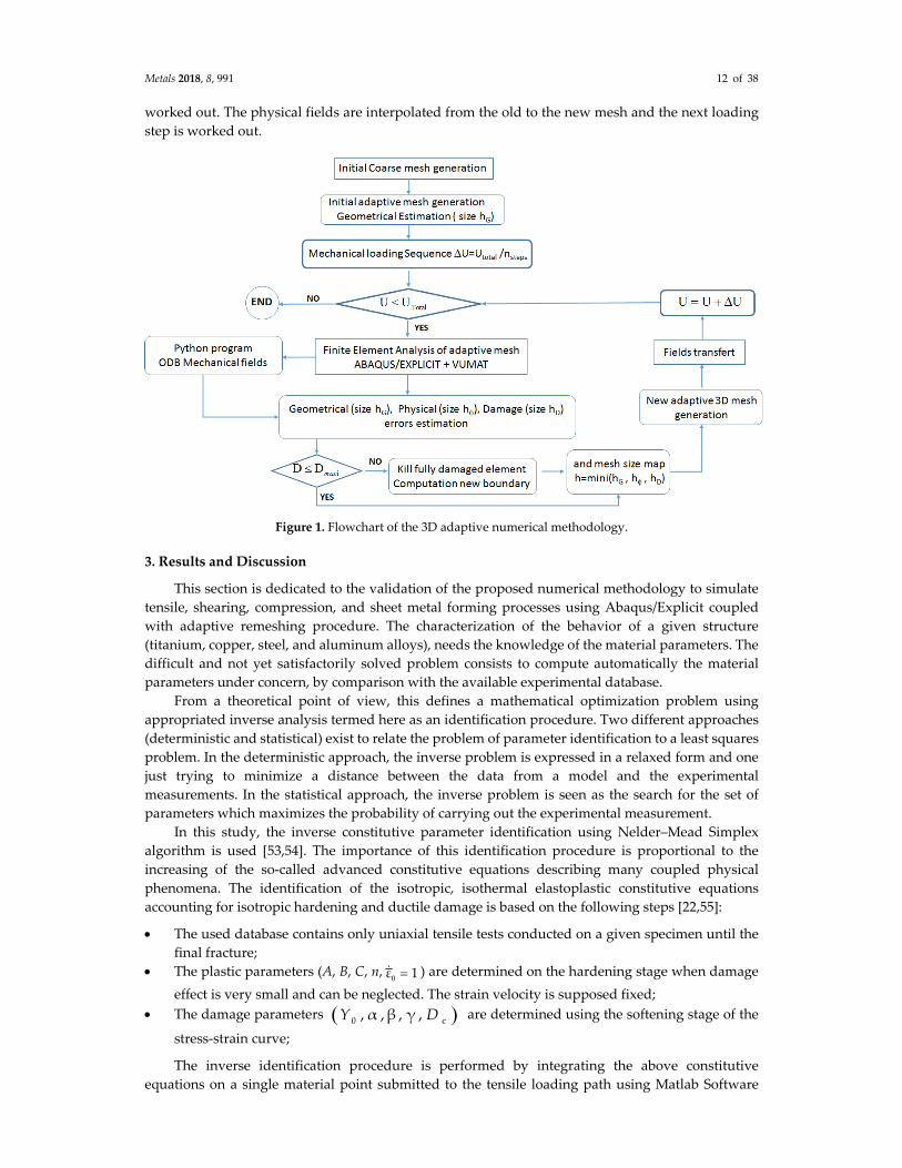
The overall adaptive methodology is implemented in the Optiform mesher package (see Figure

1). It includes the remeshing strategy, the interpolation error and the field transfer from the old mesh

to the new one. For the simulations of sheet metal forming processes, a special procedure has been

developed in order to execute Abaqus software [47] step by step. At each load increment, and after

the convergence has been reached, the overall elements are tested in order to detect the fully damaged

elements (elements where the damage variable has reach its critical value in all Gauss points). If so,

the fully damaged element is removed from the structure and a new adaptive meshing of the part is

Metals 2018, 8, 991 12 of 38

worked out. The physical fields are interpolated from the old to the new mesh and the next loading

step is worked out.

Figure 1. Flowchart of the 3D adaptive numerical methodology.

3. Results and Discussion

This section is dedicated to the validation of the proposed numerical methodology to simulate

tensile, shearing, compression, and sheet metal forming processes using Abaqus/Explicit coupled

with adaptive remeshing procedure. The characterization of the behavior of a given structure

(titanium, copper, steel, and aluminum alloys), needs the knowledge of the material parameters. The

difficult and not yet satisfactorily solved problem consists to compute automatically the material

parameters under concern, by comparison with the available experimental database.

From a theoretical point of view, this defines a mathematical optimization problem using

appropriated inverse analysis termed here as an identification procedure. Two different approaches

(deterministic and statistical) exist to relate the problem of parameter identification to a least squares

problem. In the deterministic approach, the inverse problem is expressed in a relaxed form and one

just trying to minimize a distance between the data from a model and the experimental

measurements. In the statistical approach, the inverse problem is seen as the search for the set of

parameters which maximizes the probability of carrying out the experimental measurement.

In this study, the inverse constitutive parameter identification using Nelder–Mead Simplex

algorithm is used [53,54]. The importance of this identification procedure is proportional to the

increasing of the so-called advanced constitutive equations describing many coupled physical

phenomena. The identification of the isotropic, isothermal elastoplastic constitutive equations

accounting for isotropic hardening and ductile damage is based on the following steps [22,55]:

The used database contains only uniaxial tensile tests conducted on a given specimen until the

final fracture;

The plastic parameters (A, B, C, n,0ε 1 ) are determined on the hardening stage when damage

effect is very small and can be neglected. The strain velocity is supposed fixed;

The damage parameters 0 c, α , β , γ ,Y D are determined using the softening stage of the

stress-strain curve;

The inverse identification procedure is performed by integrating the above constitutive

equations on a single material point submitted to the tensile loading path using Matlab Software

Metals 2018, 8, 991 13 of 38

(Nelder–Mead Simplex algorithm) and the user’s subroutine. Using material parameters determined

above, the real specimen in tensile, shear or compression test is simulated by FEA and the global

force-displacement curve is compared to the experimental one. If needed, the material parameters

are adjusted and new FEA simulations are performed until the experimental and numerical force-

displacement curves compares well.

Some obvious phenomena, like strain localization and damage evolutions, were presented in

order to test the capability of the proposed fully coupled model and adaptive remeshing scheme to

simulate the sheet metal forming process like blanking, multi-point drawing, single incremental

forming and deep-drawing. All the numerical simulation are performed on the Dell Precision T7600

Workstation, 2× Intel Xeon E5-2670 2.6 GHz 4 CPU Cores Processors; 128 GB Memory, Ubuntu Linux

64Mbit.

3.1. Uniaxial Tensile Test of XES Steel Sheet

The proposed constitutive equations are used to predict the stress-strain curve of XES steel

which is used in the tensile experiment [20]. The fully coupled damage constitutive equations are

implemented to predict the maximum stress maxσ = 383 MPa , the plastic strain at damage initiation

c

pε = 0.22 and the plastic strain to fracture max

pε = 0.26 . The damage evolves from the damage

initiation to the fracture Dmax = 0.99 and the material stiffness degrades from maximum tensile force

to zero. The best parameters found to fit the experiment stress-strain curve are shown in Table 1. The

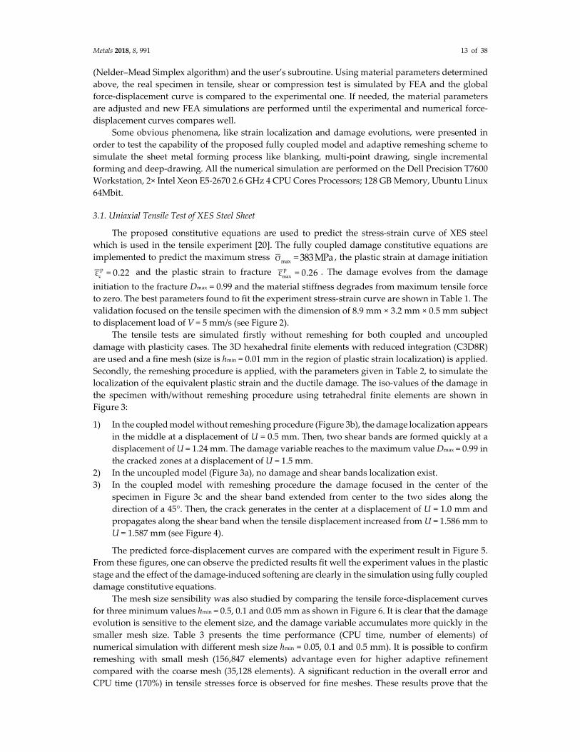
validation focused on the tensile specimen with the dimension of 8.9 mm × 3.2 mm × 0.5 mm subject

to displacement load of V = 5 mm/s (see Figure 2).

The tensile tests are simulated firstly without remeshing for both coupled and uncoupled

damage with plasticity cases. The 3D hexahedral finite elements with reduced integration (C3D8R)

are used and a fine mesh (size is hmin = 0.01 mm in the region of plastic strain localization) is applied.

Secondly, the remeshing procedure is applied, with the parameters given in Table 2, to simulate the

localization of the equivalent plastic strain and the ductile damage. The iso-values of the damage in

the specimen with/without remeshing procedure using tetrahedral finite elements are shown in

Figure 3:

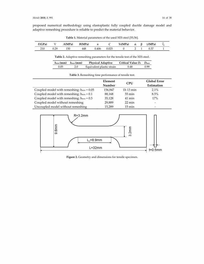
1) In the coupled model without remeshing procedure (Figure 3b), the damage localization appears

in the middle at a displacement of U = 0.5 mm. Then, two shear bands are formed quickly at a

displacement of U = 1.24 mm. The damage variable reaches to the maximum value Dmax = 0.99 in

the cracked zones at a displacement of U = 1.5 mm.

2) In the uncoupled model (Figure 3a), no damage and shear bands localization exist.

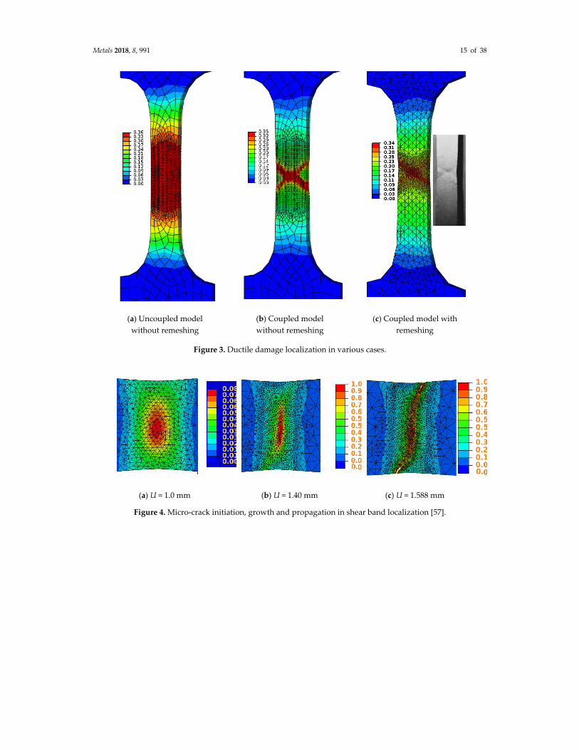
3) In the coupled model with remeshing procedure the damage focused in the center of the

specimen in Figure 3c and the shear band extended from center to the two sides along the

direction of a 45°. Then, the crack generates in the center at a displacement of U = 1.0 mm and

propagates along the shear band when the tensile displacement increased from U = 1.586 mm to

U = 1.587 mm (see Figure 4).

The predicted force-displacement curves are compared with the experiment result in Figure 5.

From these figures, one can observe the predicted results fit well the experiment values in the plastic

stage and the effect of the damage-induced softening are clearly in the simulation using fully coupled

damage constitutive equations.

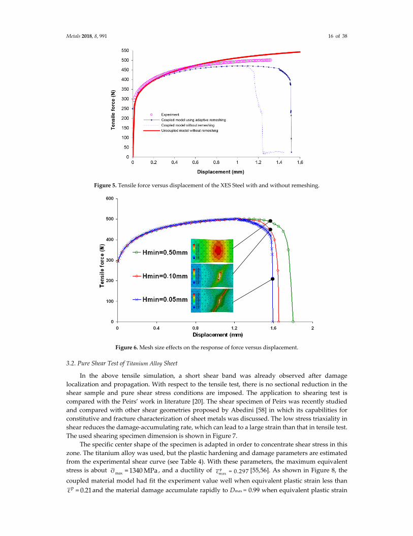
The mesh size sensibility was also studied by comparing the tensile force-displacement curves

for three minimum values hmin = 0.5, 0.1 and 0.05 mm as shown in Figure 6. It is clear that the damage

evolution is sensitive to the element size, and the damage variable accumulates more quickly in the

smaller mesh size. Table 3 presents the time performance (CPU time, number of elements) of

numerical simulation with different mesh size hmin = 0.05, 0.1 and 0.5 mm). It is possible to confirm

remeshing with small mesh (156,847 elements) advantage even for higher adaptive refinement

compared with the coarse mesh (35,128 elements). A significant reduction in the overall error and

CPU time (170%) in tensile stresses force is observed for fine meshes. These results prove that the

Metals 2018, 8, 991 14 of 38

proposed numerical methodology using elastoplastic fully coupled ductile damage model and

adaptive remeshing procedure is reliable to predict the material behavior.

Table 1. Material parameters of the used XES steel [55,56].

E(GPa) ν A(MPa) B(MPa) n C Y0(MPa) α β γ(MPa) 0ε

210 0.29 150 448 0.406 0.025 0 2 1 0.37 1

Table 2. Adaptive remeshing parameters for the tensile test of the XES steel.

hmin (mm) hmax (mm) Physical Adaptive Critical Value Dc Dmax

0.05 2.0 Equivalent plastic strain 0.48 0.99

Table 3. Remeshing time performance of tensile test.

Element

Number CPU

Global Error

Estimation

Coupled model with remeshing: hmin = 0.05 156,847 1h 13 min 2.1%

Coupled model with remeshing: hmin = 0.1 88,168 55 min 8.5%

Coupled model with remeshing: hmin = 0.5 35,128 41 min 17%

Coupled model without remeshing 29,889 22 min -

Uncoupled model without remeshing 15,289 15 min -

Figure 2. Geometry and dimensions for tensile specimen.

Metals 2018, 8, 991 15 of 38

(a) Uncoupled model

without remeshing

(b) Coupled model

without remeshing

(c) Coupled model with

remeshing

Figure 3. Ductile damage localization in various cases.

(a) U = 1.0 mm (b) U = 1.40 mm (c) U = 1.588 mm

Figure 4. Micro-crack initiation, growth and propagation in shear band localization [57].

Metals 2018, 8, 991 16 of 38

Figure 5. Tensile force versus displacement of the XES Steel with and without remeshing.

Figure 6. Mesh size effects on the response of force versus displacement.

3.2. Pure Shear Test of Titanium Alloy Sheet

In the above tensile simulation, a short shear band was already observed after damage

localization and propagation. With respect to the tensile test, there is no sectional reduction in the

shear sample and pure shear stress conditions are imposed. The application to shearing test is

compared with the Peirs’ work in literature [20]. The shear specimen of Peirs was recently studied

and compared with other shear geometries proposed by Abedini [58] in which its capabilities for

constitutive and fracture characterization of sheet metals was discussed. The low stress triaxiality in

shear reduces the damage-accumulating rate, which can lead to a large strain than that in tensile test.

The used shearing specimen dimension is shown in Figure 7.

The specific center shape of the specimen is adapted in order to concentrate shear stress in this

zone. The titanium alloy was used, but the plastic hardening and damage parameters are estimated

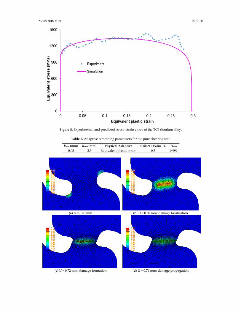
from the experimental shear curve (see Table 4). With these parameters, the maximum equivalent

stress is about maxσ = 1340 MPa , and a ductility of p

maxε = 0.297 [55,56]. As shown in Figure 8, the

coupled material model had fit the experiment value well when equivalent plastic strain less than pε = 0.21and the material damage accumulate rapidly to Dmax = 0.99 when equivalent plastic strain

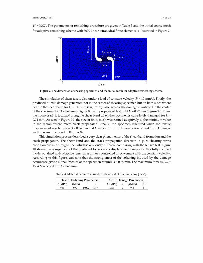
Metals 2018, 8, 991 17 of 38

pε = 0.297 . The parameters of remeshing procedure are given in Table 5 and the initial coarse mesh

for adaptive remeshing scheme with 3000 linear tetrahedral finite elements is illustrated in Figure 7.

Figure 7. The dimension of shearing specimen and the initial mesh for adaptive remeshing scheme.

The simulation of shear test is also under a load of constant velocity (V = 10 mm/s). Firstly, the

predicted ductile damage generated not in the center of shearing specimen but on both sides where

near to the shear band for U = 0.40 mm (Figure 9a). Afterwards, the damage is initiated in the center

of the specimen for U = 0.60 mm (Figure 8b) and propagated fast until U = 0.72 mm (Figure 9c). Then,

the micro-crack is localized along the shear band when the specimen is completely damaged for U =

0.74 mm. As seen in Figure 9d, the size of finite mesh was refined adaptively to the minimum value

in the region where micro-crack propagated. Finally, the specimen fractured when the tensile

displacement was between U = 0.74 mm and U = 0.75 mm. The damage variable and the 3D damage

section were illustrated in Figures 9e.

This simulation process described a very clear phenomenon of the shear band formation and the

crack propagation. The shear band and the crack propagation direction in pure shearing stress

condition are in a straight line, which is obviously different comparing with the tensile test. Figure

10 shows the comparison of the predicted force versus displacement curves for this fully coupled

model obtained with adaptive remeshing under a controlled displacement with the constant velocity.

According to this figure, can note that the strong effect of the softening induced by the damage

occurrence giving a final fracture of the specimen around U = 0.75 mm. The maximum force is Fmax =

1504 N reached for U = 0.68 mm.

Table 4. Material parameters used for shear test of titanium alloy [55,56].

Plastic Hardening Parameters Ductile Damage Parameters

A(MPa) B(MPa) C n Y0(MPa) α γ(MPa) β

951 892 0.027 0.37 0.15 2 9.3 1

Metals 2018, 8, 991 18 of 38

Figure 8. Experimental and predicted stress–strain curve of the TC4 titanium alloy.

Table 5. Adaptive remeshing parameters for the pure shearing test.

hmin (mm) hmax (mm) Physical Adaptive Critical Value Dc Dmax

0.05 2.5 Equivalent plastic strain 0.3 0.999

(a) U = 0.40 mm (b) U = 0.60 mm: damage localisation

(c) U = 0.72 mm: damage formation (d) U = 0.74 mm: damage propagation

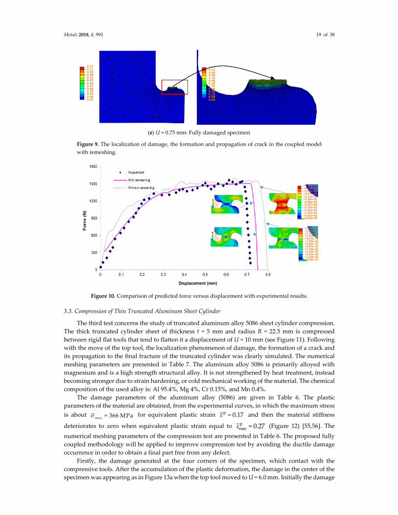
Metals 2018, 8, 991 19 of 38

Figure 9. The localization of damage, the formation and propagation of crack in the coupled model

with remeshing.

Figure 10. Comparison of predicted force versus displacement with experimental results.

3.3. Compression of Thin Truncated Aluminum Sheet Cylinder

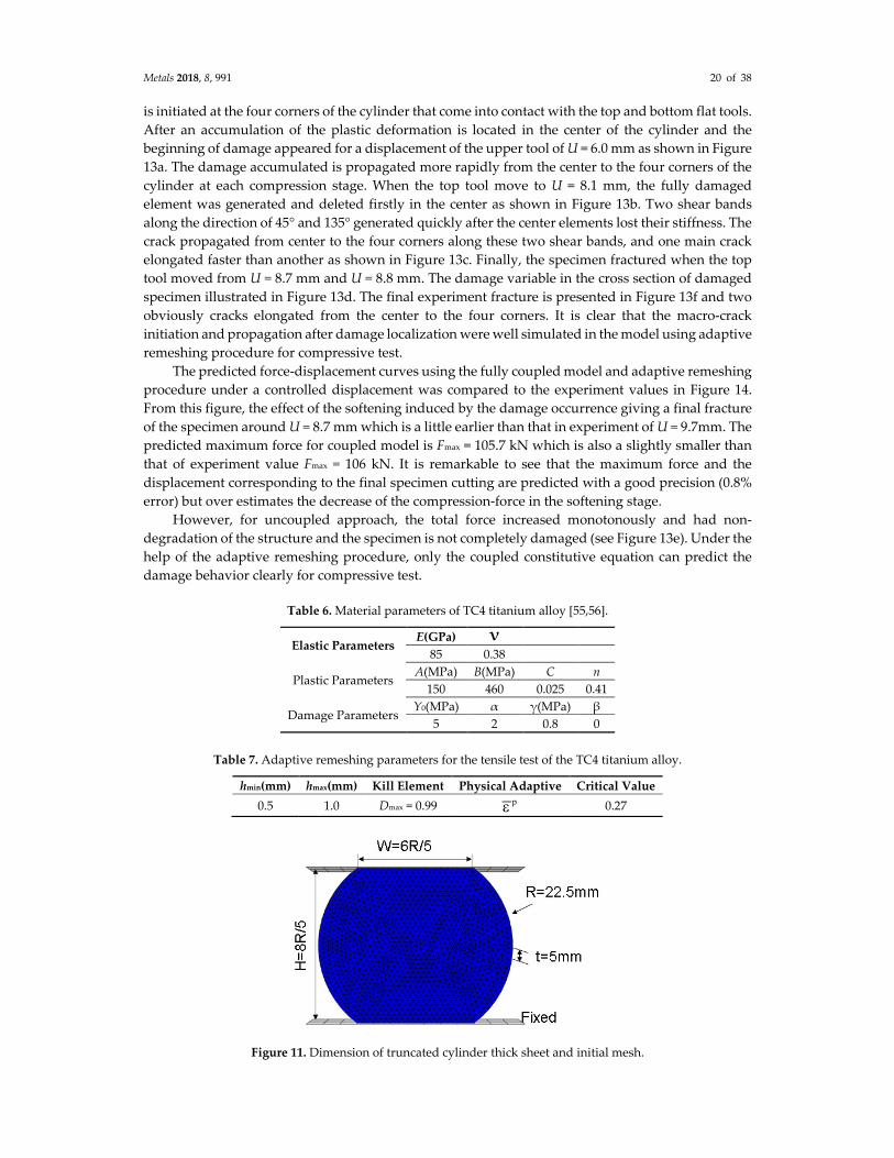
The third test concerns the study of truncated aluminum alloy 5086 sheet cylinder compression.

The thick truncated cylinder sheet of thickness t = 5 mm and radius R = 22.5 mm is compressed

between rigid flat tools that tend to flatten it a displacement of U = 10 mm (see Figure 11). Following

with the move of the top tool, the localization phenomenon of damage, the formation of a crack and

its propagation to the final fracture of the truncated cylinder was clearly simulated. The numerical

meshing parameters are presented in Table 7. The aluminum alloy 5086 is primarily alloyed with

magnesium and is a high strength structural alloy. It is not strengthened by heat treatment, instead

becoming stronger due to strain hardening, or cold mechanical working of the material. The chemical

composition of the used alloy is: Al 95.4%, Mg 4%, Cr 0.15%, and Mn 0.4%.

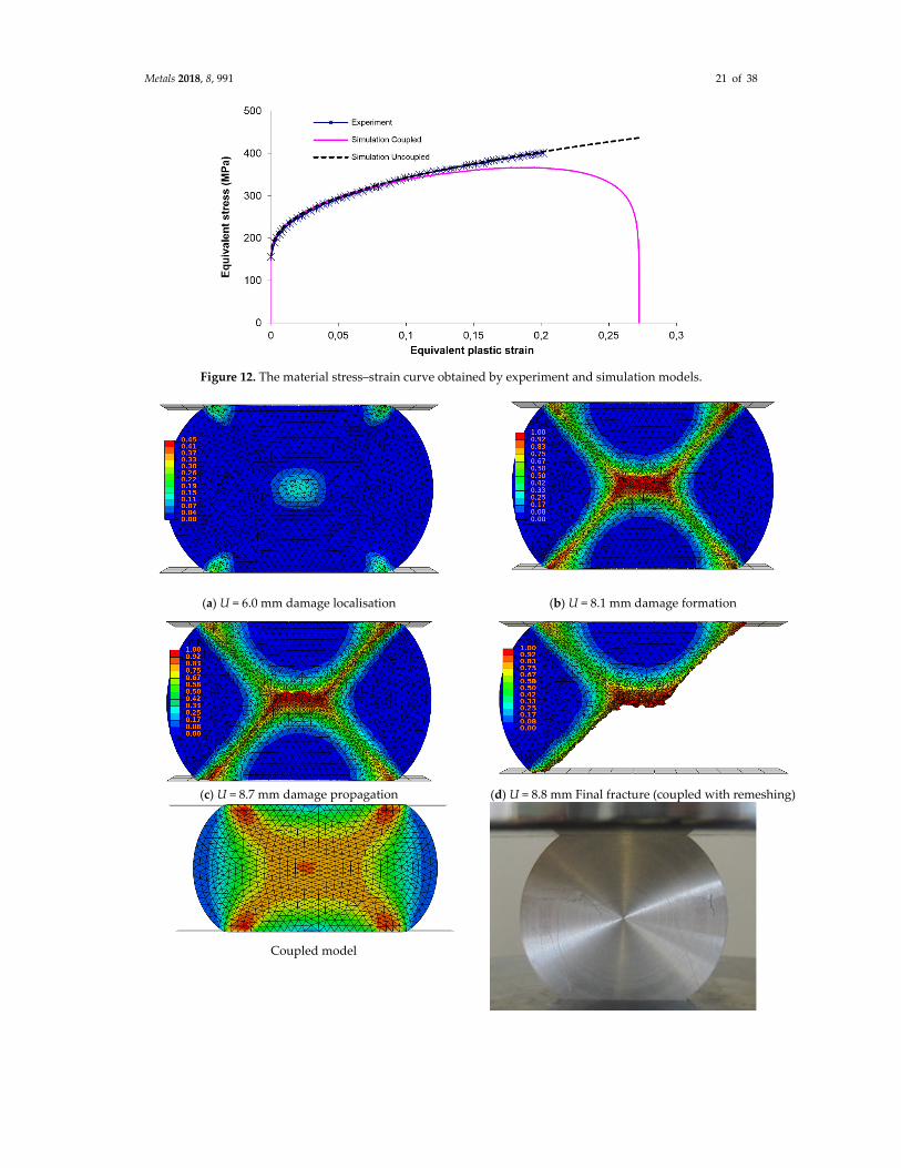
The damage parameters of the aluminum alloy (5086) are given in Table 6. The plastic

parameters of the material are obtained, from the experimental curves, in which the maximum stress

is about maxσ = 366 MPa for equivalent plastic strain pε = 0.17 and then the material stiffness

deteriorates to zero when equivalent plastic strain equal to pmaxε = 0.27 (Figure 12) [55,56]. The

numerical meshing parameters of the compression test are presented in Table 6. The proposed fully

coupled methodology will be applied to improve compression test by avoiding the ductile damage

occurrence in order to obtain a final part free from any defect.

Firstly, the damage generated at the four corners of the specimen, which contact with the

compressive tools. After the accumulation of the plastic deformation, the damage in the center of the

specimen was appearing as in Figure 13a when the top tool moved to U = 6.0 mm. Initially the damage

(e) U = 0.75 mm: Fully damaged specimen

Metals 2018, 8, 991 20 of 38

is initiated at the four corners of the cylinder that come into contact with the top and bottom flat tools.

After an accumulation of the plastic deformation is located in the center of the cylinder and the

beginning of damage appeared for a displacement of the upper tool of U = 6.0 mm as shown in Figure

13a. The damage accumulated is propagated more rapidly from the center to the four corners of the

cylinder at each compression stage. When the top tool move to U = 8.1 mm, the fully damaged

element was generated and deleted firstly in the center as shown in Figure 13b. Two shear bands

along the direction of 45° and 135° generated quickly after the center elements lost their stiffness. The

crack propagated from center to the four corners along these two shear bands, and one main crack

elongated faster than another as shown in Figure 13c. Finally, the specimen fractured when the top

tool moved from U = 8.7 mm and U = 8.8 mm. The damage variable in the cross section of damaged

specimen illustrated in Figure 13d. The final experiment fracture is presented in Figure 13f and two

obviously cracks elongated from the center to the four corners. It is clear that the macro-crack

initiation and propagation after damage localization were well simulated in the model using adaptive

remeshing procedure for compressive test.

The predicted force-displacement curves using the fully coupled model and adaptive remeshing

procedure under a controlled displacement was compared to the experiment values in Figure 14.

From this figure, the effect of the softening induced by the damage occurrence giving a final fracture

of the specimen around U = 8.7 mm which is a little earlier than that in experiment of U = 9.7mm. The

predicted maximum force for coupled model is Fmax = 105.7 kN which is also a slightly smaller than

that of experiment value Fmax = 106 kN. It is remarkable to see that the maximum force and the

displacement corresponding to the final specimen cutting are predicted with a good precision (0.8%

error) but over estimates the decrease of the compression-force in the softening stage.

However, for uncoupled approach, the total force increased monotonously and had non-

degradation of the structure and the specimen is not completely damaged (see Figure 13e). Under the

help of the adaptive remeshing procedure, only the coupled constitutive equation can predict the

damage behavior clearly for compressive test.

Table 6. Material parameters of TC4 titanium alloy [55,56].

Elastic Parameters E(GPa) ν

85 0.38

Plastic Parameters A(MPa) B(MPa) C n

150 460 0.025 0.41

Damage Parameters Y0(MPa) α γ(MPa) β

5 2 0.8 0

Table 7. Adaptive remeshing parameters for the tensile test of the TC4 titanium alloy.

hmin(mm) hmax(mm) Kill Element Physical Adaptive Critical Value

0.5 1.0 Dmax = 0.99 p 0.27

Figure 11. Dimension of truncated cylinder thick sheet and initial mesh.

Metals 2018, 8, 991 21 of 38

Figure 12. The material stress–strain curve obtained by experiment and simulation models.

(a) U = 6.0 mm damage localisation (b) U = 8.1 mm damage formation

(c) U = 8.7 mm damage propagation (d) U = 8.8 mm Final fracture (coupled with remeshing)

Coupled model

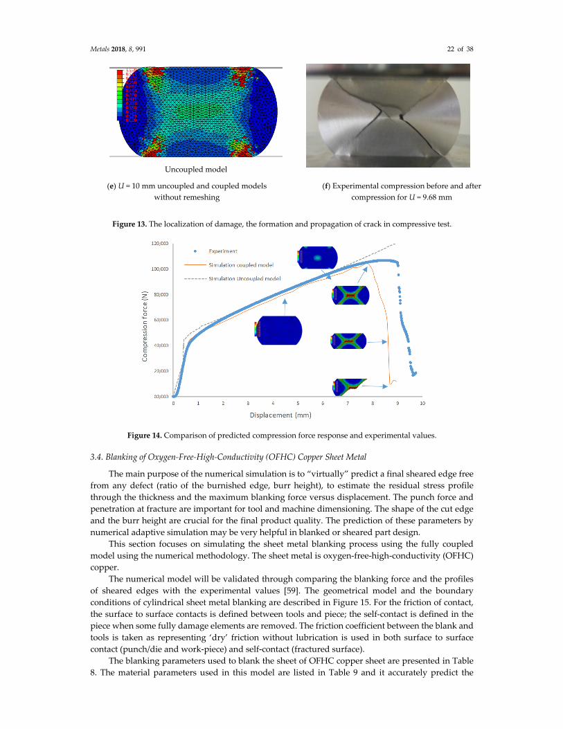
Metals 2018, 8, 991 22 of 38

Uncoupled model

(e) U = 10 mm uncoupled and coupled models

without remeshing

(f) Experimental compression before and after

compression for U = 9.68 mm

Figure 13. The localization of damage, the formation and propagation of crack in compressive test.

Figure 14. Comparison of predicted compression force response and experimental values.

3.4. Blanking of Oxygen-Free-High-Conductivity (OFHC) Copper Sheet Metal

The main purpose of the numerical simulation is to “virtually” predict a final sheared edge free

from any defect (ratio of the burnished edge, burr height), to estimate the residual stress profile

through the thickness and the maximum blanking force versus displacement. The punch force and

penetration at fracture are important for tool and machine dimensioning. The shape of the cut edge

and the burr height are crucial for the final product quality. The prediction of these parameters by

numerical adaptive simulation may be very helpful in blanked or sheared part design.

This section focuses on simulating the sheet metal blanking process using the fully coupled

model using the numerical methodology. The sheet metal is oxygen-free-high-conductivity (OFHC)

copper.

The numerical model will be validated through comparing the blanking force and the profiles

of sheared edges with the experimental values [59]. The geometrical model and the boundary

conditions of cylindrical sheet metal blanking are described in Figure 15. For the friction of contact,

the surface to surface contacts is defined between tools and piece; the self-contact is defined in the

piece when some fully damage elements are removed. The friction coefficient between the blank and

tools is taken as representing ‘dry’ friction without lubrication is used in both surface to surface

contact (punch/die and work-piece) and self-contact (fractured surface).

The blanking parameters used to blank the sheet of OFHC copper sheet are presented in Table

8. The material parameters used in this model are listed in Table 9 and it accurately predict the

Metals 2018, 8, 991 23 of 38

material behavior with a maximum stress of maxσ = 350MPa ,

pε = 0.77and max

pε = 0.9 . In order to

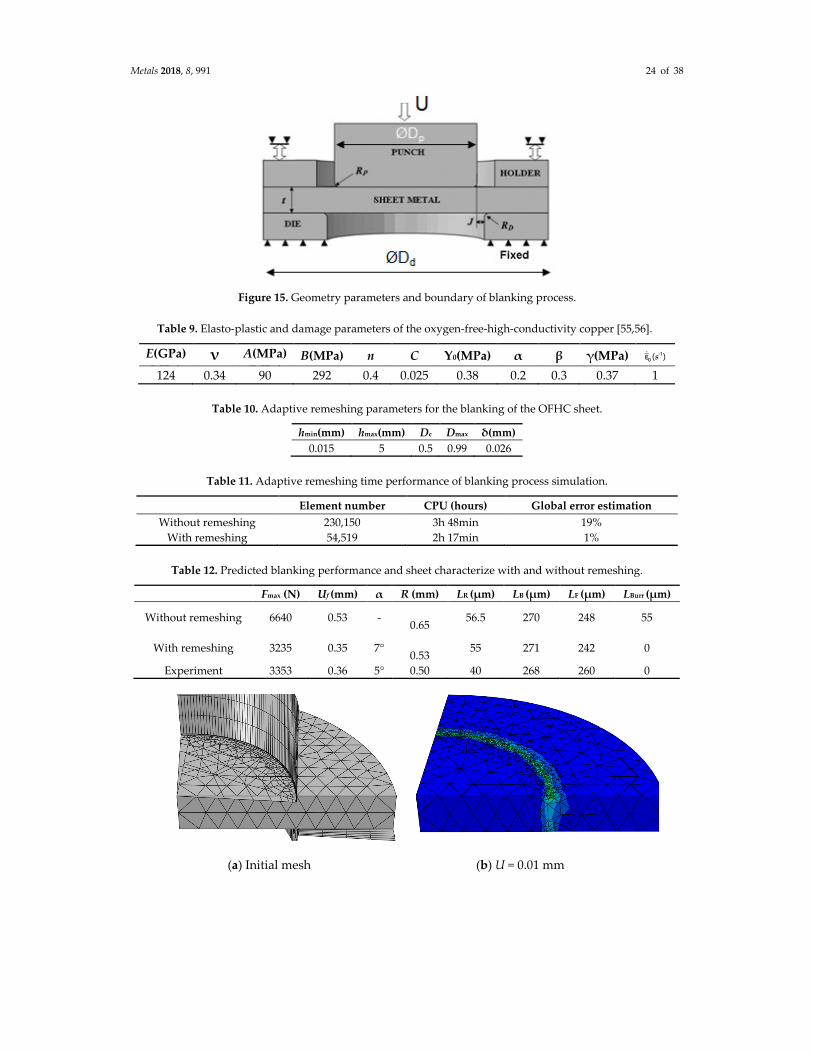
save the computing cost, quarter of the round sheet is considered. The round sheet is initially

discretized by a very coarse mesh (453 linear tetrahedral elements as shown in Figure 16a).

Geometrical error estimation and the contact region with tools (punch and die) with respect the

minimum size hmin then control the adaptive mesh (Table 10). In the following steps, the mesh

regenerates adaptively according to the plastic strain and the damage variable. When the damage

accumulates Dmax > 0.99, the element will be removed and a new boundary will be generated. The

macro-crack initiation and propagation during the sheet blanking were analyzed at each punch

penetration in Figure 16b for U = 0.01 mm and in Figure 16c for U = 0.2 mm. The copper sheet was

fully cut for U = 0.33 mm.

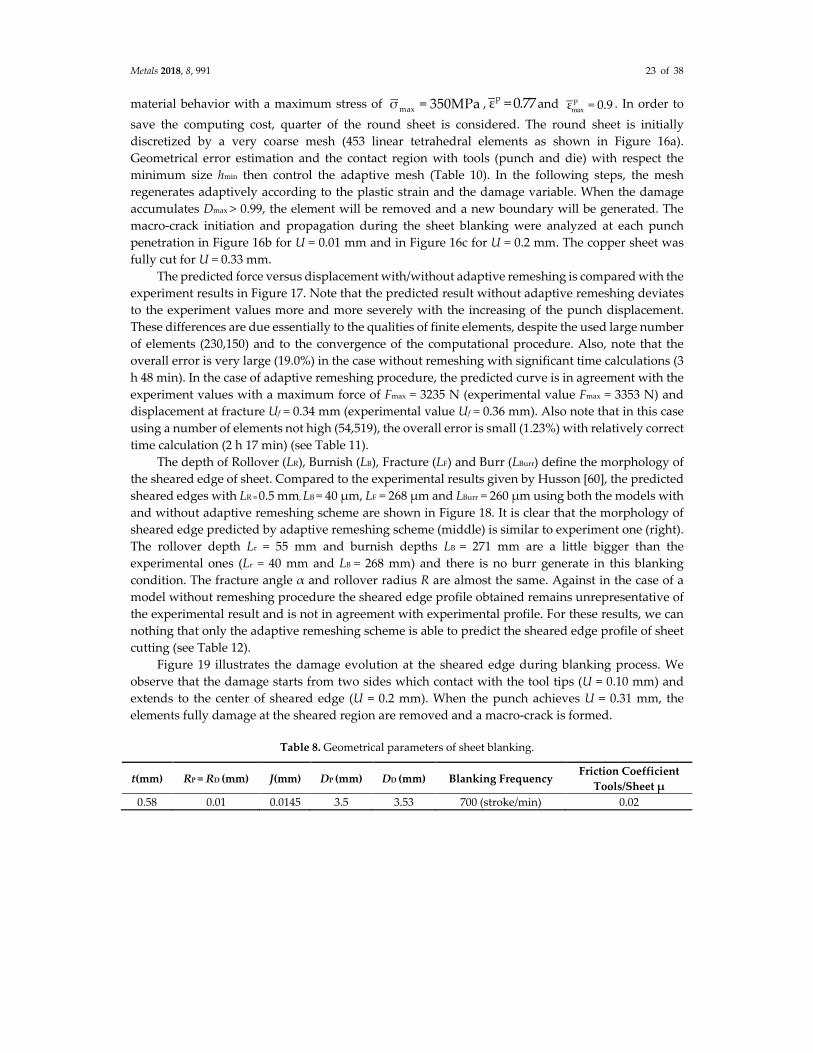
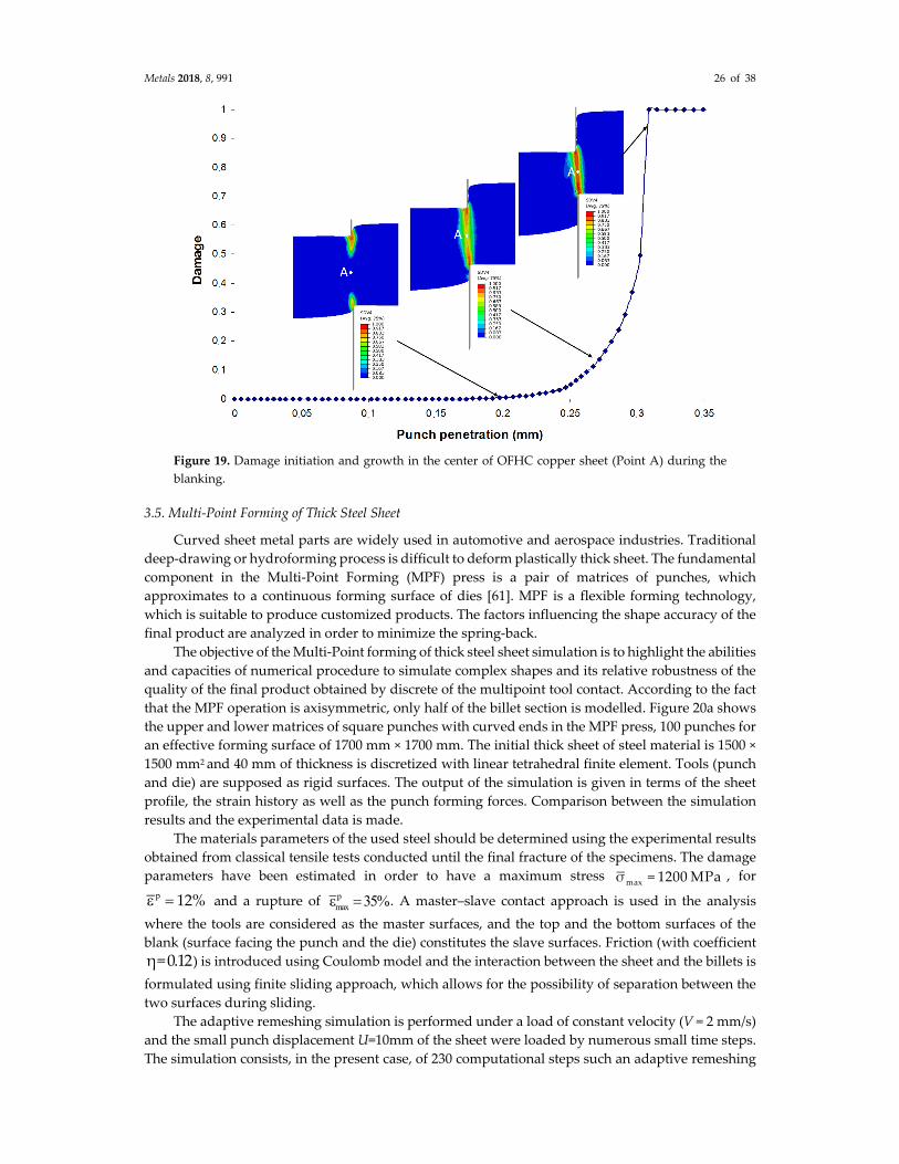
The predicted force versus displacement with/without adaptive remeshing is compared with the

experiment results in Figure 17. Note that the predicted result without adaptive remeshing deviates

to the experiment values more and more severely with the increasing of the punch displacement.

These differences are due essentially to the qualities of finite elements, despite the used large number

of elements (230,150) and to the convergence of the computational procedure. Also, note that the

overall error is very large (19.0%) in the case without remeshing with significant time calculations (3

h 48 min). In the case of adaptive remeshing procedure, the predicted curve is in agreement with the

experiment values with a maximum force of Fmax = 3235 N (experimental value Fmax = 3353 N) and

displacement at fracture Uf = 0.34 mm (experimental value Uf = 0.36 mm). Also note that in this case

using a number of elements not high (54,519), the overall error is small (1.23%) with relatively correct

time calculation (2 h 17 min) (see Table 11).

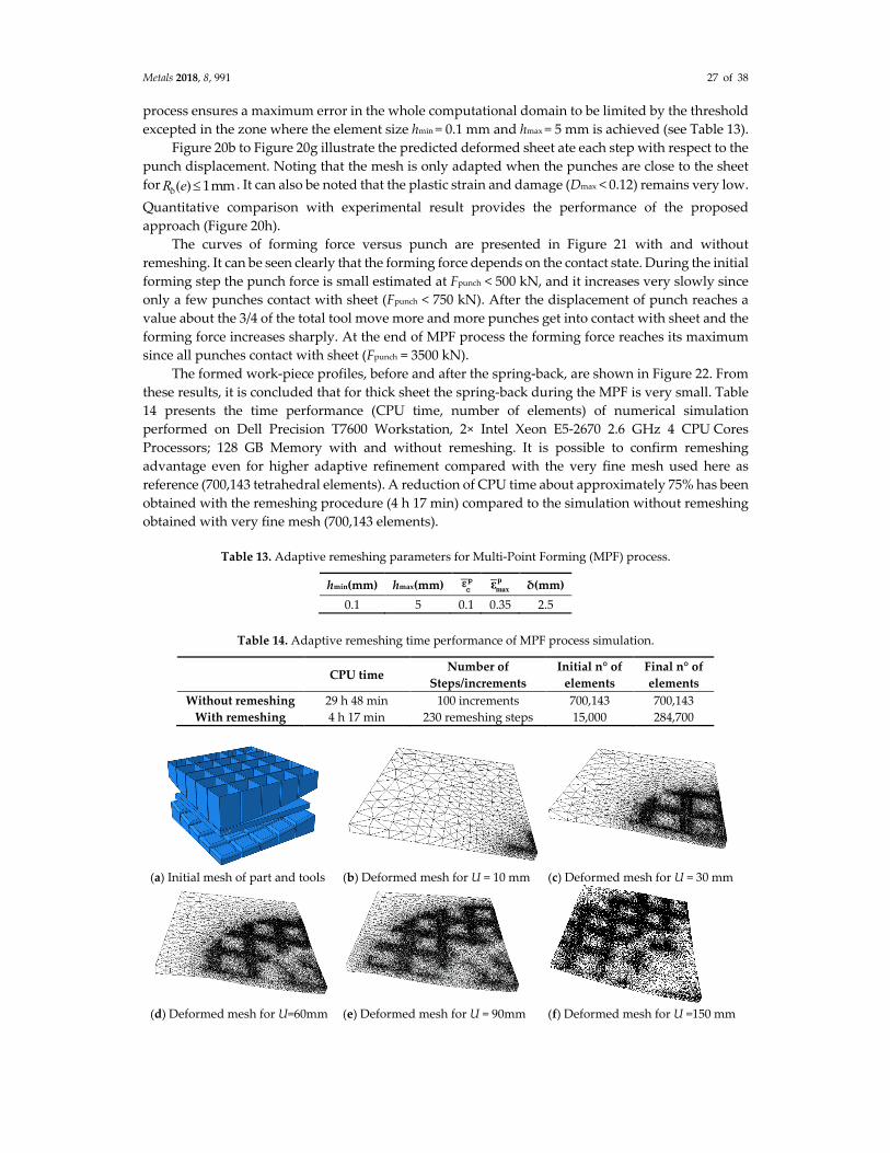
The depth of Rollover (LR), Burnish (LB), Fracture (LF) and Burr (LBurr) define the morphology of

the sheared edge of sheet. Compared to the experimental results given by Husson [60], the predicted

sheared edges with LR = 0.5 mm, LB = 40 μm, LF = 268 μm and LBurr = 260 μm using both the models with

and without adaptive remeshing scheme are shown in Figure 18. It is clear that the morphology of

sheared edge predicted by adaptive remeshing scheme (middle) is similar to experiment one (right).

The rollover depth Lr = 55 mm and burnish depths LB = 271 mm are a little bigger than the

experimental ones (Lr = 40 mm and LB = 268 mm) and there is no burr generate in this blanking

condition. The fracture angle α and rollover radius R are almost the same. Against in the case of a

model without remeshing procedure the sheared edge profile obtained remains unrepresentative of

the experimental result and is not in agreement with experimental profile. For these results, we can

nothing that only the adaptive remeshing scheme is able to predict the sheared edge profile of sheet

cutting (see Table 12).

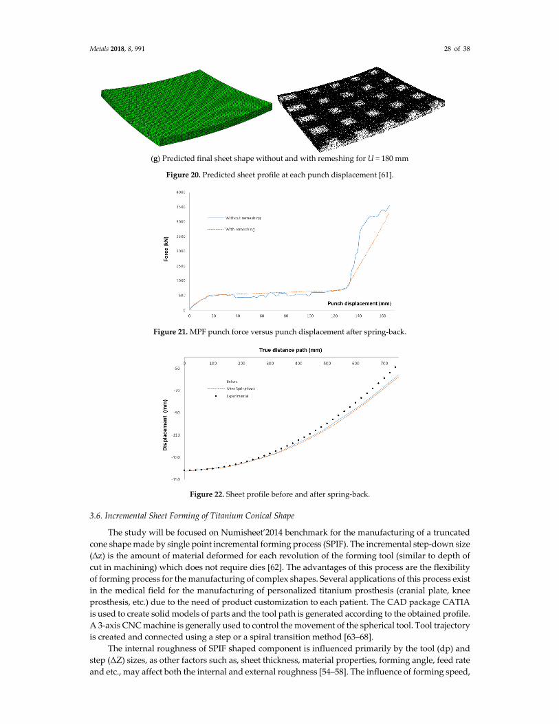
Figure 19 illustrates the damage evolution at the sheared edge during blanking process. We

observe that the damage starts from two sides which contact with the tool tips (U = 0.10 mm) and

extends to the center of sheared edge (U = 0.2 mm). When the punch achieves U = 0.31 mm, the

elements fully damage at the sheared region are removed and a macro-crack is formed.

Table 8. Geometrical parameters of sheet blanking.

t(mm) RP = RD (mm) J(mm) DP (mm) DD (mm) Blanking Frequency Friction Coefficient

Tools/Sheet µ

0.58 0.01 0.0145 3.5 3.53 700 (stroke/min) 0.02

Metals 2018, 8, 991 24 of 38

Figure 15. Geometry parameters and boundary of blanking process.

Table 9. Elasto-plastic and damage parameters of the oxygen-free-high-conductivity copper [55,56].

E(GPa)

MPa) ν A(MPa)

(MPa) B(MPa) n C Y0(MPa) α β γ(MPa) -1

0ε ( )s

124 0.34 90 292 0.4 0.025 0.38 0.2 0.3 0.37 1

Table 10. Adaptive remeshing parameters for the blanking of the OFHC sheet.

hmin(mm) hmax(mm) Dc Dmax δ(mm)

0.015 5 0.5 0.99 0.026

Table 11. Adaptive remeshing time performance of blanking process simulation.

Element number CPU (hours) Global error estimation

Without remeshing 230,150 3h 48min 19%

With remeshing 54,519 2h 17min 1%

Table 12. Predicted blanking performance and sheet characterize with and without remeshing.

Fmax (N) Uf (mm) α R (mm) LR (µm) LB (µm) LF (µm) LBurr (µm)

Without remeshing 6640 0.53 -

0.65 56.5 270 248 55

With remeshing 3235 0.35 7°

0.53 55 271 242 0

Experiment 3353 0.36 5° 0.50 40 268 260 0

(a) Initial mesh (b) U = 0.01 mm

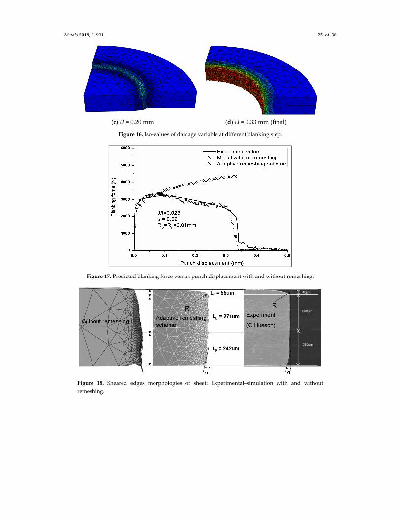
Metals 2018, 8, 991 25 of 38

(c) U = 0.20 mm (d) U = 0.33 mm (final)

Figure 16. Iso-values of damage variable at different blanking step.

Figure 17. Predicted blanking force versus punch displacement with and without remeshing.

Figure 18. Sheared edges morphologies of sheet: Experimental–simulation with and without

remeshing.

Metals 2018, 8, 991 26 of 38

Figure 19. Damage initiation and growth in the center of OFHC copper sheet (Point A) during the

blanking.

3.5. Multi-Point Forming of Thick Steel Sheet

Curved sheet metal parts are widely used in automotive and aerospace industries. Traditional

deep-drawing or hydroforming process is difficult to deform plastically thick sheet. The fundamental

component in the Multi-Point Forming (MPF) press is a pair of matrices of punches, which

approximates to a continuous forming surface of dies [61]. MPF is a flexible forming technology,

which is suitable to produce customized products. The factors influencing the shape accuracy of the

final product are analyzed in order to minimize the spring-back.

The objective of the Multi-Point forming of thick steel sheet simulation is to highlight the abilities

and capacities of numerical procedure to simulate complex shapes and its relative robustness of the

quality of the final product obtained by discrete of the multipoint tool contact. According to the fact

that the MPF operation is axisymmetric, only half of the billet section is modelled. Figure 20a shows

the upper and lower matrices of square punches with curved ends in the MPF press, 100 punches for

an effective forming surface of 1700 mm × 1700 mm. The initial thick sheet of steel material is 1500 ×

1500 mm2 and 40 mm of thickness is discretized with linear tetrahedral finite element. Tools (punch

and die) are supposed as rigid surfaces. The output of the simulation is given in terms of the sheet

profile, the strain history as well as the punch forming forces. Comparison between the simulation

results and the experimental data is made.

The materials parameters of the used steel should be determined using the experimental results

obtained from classical tensile tests conducted until the final fracture of the specimens. The damage

parameters have been estimated in order to have a maximum stress maxσ = 1200 MPa , for

p 12% and a rupture of pmax 35% . A master–slave contact approach is used in the analysis

where the tools are considered as the master surfaces, and the top and the bottom surfaces of the

blank (surface facing the punch and the die) constitutes the slave surfaces. Friction (with coefficient

η=0.12) is introduced using Coulomb model and the interaction between the sheet and the billets is

formulated using finite sliding approach, which allows for the possibility of separation between the

two surfaces during sliding.

The adaptive remeshing simulation is performed under a load of constant velocity (V = 2 mm/s)

and the small punch displacement U=10mm of the sheet were loaded by numerous small time steps.

The simulation consists, in the present case, of 230 computational steps such an adaptive remeshing

Metals 2018, 8, 991 27 of 38

process ensures a maximum error in the whole computational domain to be limited by the threshold

excepted in the zone where the element size hmin = 0.1 mm and hmax = 5 mm is achieved (see Table 13).

Figure 20b to Figure 20g illustrate the predicted deformed sheet ate each step with respect to the

punch displacement. Noting that the mesh is only adapted when the punches are close to the sheet

for ( )δ 1 mmeR . It can also be noted that the plastic strain and damage (Dmax < 0.12) remains very low.

Quantitative comparison with experimental result provides the performance of the proposed

approach (Figure 20h).

The curves of forming force versus punch are presented in Figure 21 with and without

remeshing. It can be seen clearly that the forming force depends on the contact state. During the initial

forming step the punch force is small estimated at Fpunch < 500 kN, and it increases very slowly since

only a few punches contact with sheet (Fpunch < 750 kN). After the displacement of punch reaches a

value about the 3/4 of the total tool move more and more punches get into contact with sheet and the

forming force increases sharply. At the end of MPF process the forming force reaches its maximum

since all punches contact with sheet (Fpunch = 3500 kN).

The formed work-piece profiles, before and after the spring-back, are shown in Figure 22. From

these results, it is concluded that for thick sheet the spring-back during the MPF is very small. Table

14 presents the time performance (CPU time, number of elements) of numerical simulation

performed on Dell Precision T7600 Workstation, 2× Intel Xeon E5-2670 2.6 GHz 4 CPU Cores

Processors; 128 GB Memory with and without remeshing. It is possible to confirm remeshing

advantage even for higher adaptive refinement compared with the very fine mesh used here as

reference (700,143 tetrahedral elements). A reduction of CPU time about approximately 75% has been

obtained with the remeshing procedure (4 h 17 min) compared to the simulation without remeshing

obtained with very fine mesh (700,143 elements).

Table 13. Adaptive remeshing parameters for Multi-Point Forming (MPF) process.

hmin(mm) hmax(mm) pcε p

maxε δ(mm)

0.1 5 0.1 0.35 2.5

Table 14. Adaptive remeshing time performance of MPF process simulation.

CPU time Number of

Steps/increments

Initial n° of

elements

Final n° of

elements

Without remeshing 29 h 48 min 100 increments 700,143 700,143

With remeshing 4 h 17 min 230 remeshing steps 15,000 284,700

(a) Initial mesh of part and tools (b) Deformed mesh for U = 10 mm (c) Deformed mesh for U = 30 mm

(d) Deformed mesh for U=60mm (e) Deformed mesh for U = 90mm (f) Deformed mesh for U =150 mm

Metals 2018, 8, 991 28 of 38

(g) Predicted final sheet shape without and with remeshing for U = 180 mm

Figure 20. Predicted sheet profile at each punch displacement [61].

Figure 21. MPF punch force versus punch displacement after spring-back.

Figure 22. Sheet profile before and after spring-back.

3.6. Incremental Sheet Forming of Titanium Conical Shape

The study will be focused on Numisheet’2014 benchmark for the manufacturing of a truncated

cone shape made by single point incremental forming process (SPIF). The incremental step-down size

(∆z) is the amount of material deformed for each revolution of the forming tool (similar to depth of

cut in machining) which does not require dies [62]. The advantages of this process are the flexibility

of forming process for the manufacturing of complex shapes. Several applications of this process exist

in the medical field for the manufacturing of personalized titanium prosthesis (cranial plate, knee

prosthesis, etc.) due to the need of product customization to each patient. The CAD package CATIA

is used to create solid models of parts and the tool path is generated according to the obtained profile.

A 3-axis CNC machine is generally used to control the movement of the spherical tool. Tool trajectory

is created and connected using a step or a spiral transition method [63–68].

The internal roughness of SPIF shaped component is influenced primarily by the tool (dp) and

step (ΔZ) sizes, as other factors such as, sheet thickness, material properties, forming angle, feed rate

and etc., may affect both the internal and external roughness [54–58]. The influence of forming speed,

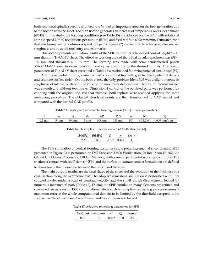
Metals 2018, 8, 991 29 of 38

both rotational spindle speed N and feed rate Vf had an important effect on the heat generation due

to the friction with the sheet. Too high friction generates an increase of temperature and sheet damage

[47,48]. In this study, the forming conditions (see Table 15) are adopted for the SPIF with rotational

spindle speed N = 40 revolutions per minute (RPM) and feed rate Vf = 6000 mm/mm. Truncated cone

that was formed using continuous spiral tool paths (Figure 22) also in order to achieve smaller surface

roughness and to avoid tool entry and exit marks.

This section presents simulation results of the SPIF to produce a truncated conical height h = 40

mm titanium Ti-6Al-4V sheet. The effective working area of the initial circular specimen was D =

130 mm and thickness ti = 0.5 mm. The forming was made with semi hemispherical punch

X160CrMoV12 steel in order to obtain prototypes according to the desired profiles. The plastic

parameters of Ti-6Al-4V sheet presented in Table 16 was obtained following uniaxial tensile tests [59].

After incremental forming, visual control is performed first with goal to detect potential defects

and estimate surface finish. On the both plates, the only problem identified was a slight increase in

roughness of internal surface in the zone of the maximum deformation. The rest of internal surface

was smooth and without tool marks. Dimensional control of the obtained parts was performed by

coupling with the original one. For that purpose, both replicas were scanned applying the same

measuring procedure. The obtained clouds of points are then transformed to CAD model and

compared with the desired CAD profile.

Table 15. Single point incremental forming process (SPIF) process parameters.

ti rc h dp ΔZ ØD α N Vf

0.5 mm 5 mm 40 mm 5 mm 0.5 mm 130 mm 50° 40 RPM 600 mm/mm

Table 16. Elasto-plastic parameters of Ti-6Al-4V sheet [60,61].

A(MPa) B(MPa) C n -10ε ( ) s

968 380 0.0197 0.421 1

The FEA simulation of conical forming design of single point incremental sheet forming SPIF

presented in Figure 23 is performed on Dell Precision T7600 Workstation, 2× Intel Xeon E5-2670 2.6

GHz 4 CPU Cores Processors; 128 GB Memory, with same experimental working conditions. The

friction of contact with coefficient η=0.14 and the surface-to-surface contact formulation are defined

to characterize the interaction between the punch and the sheet.

The main outputs results are the final shape of the sheet and the evolution of the thickness in a

cross-section along the symmetric axis. The adaptive remeshing simulation is performed with fully

coupled model under a load of constant velocity and the small punch displacement loaded by

numerous incremental path (Table 17). During the SPIF simulation many elements are refined and

coarsened, so as a result 1500 computational steps such an adaptive remeshing process ensures a

maximum error in the whole computational domain to be limited by the threshold excepted in the

zone where the element size hmin = 0.5 mm and hmax = 10 mm is achieved.

Table 17. Adaptive remeshing parameters for SPIF.

hmin(mm) hmax(mm) pcε p

maxε δ(mm)

0.15 10 0.012 0.30 2.5

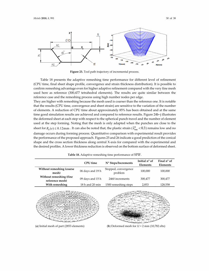
Metals 2018, 8, 991 30 of 38

Figure 23. Tool path trajectory of incremental process.

Table 18 presents the adaptive remeshing time performance for different level of refinement

(CPU time, final sheet shape profile, convergence and strain thickness distribution). It is possible to

confirm remeshing advantage even for higher adaptive refinement compared with the very fine mesh

used here as reference (300,477 tetrahedral elements). The results are quite similar between the

reference case and the remeshing process using high number nodes per edge.

They are higher with remeshing because the mesh used is coarser than the reference one. It is notable

that the results (CPU time, convergence and sheet strain) are sensitive to the variation of the number

of elements. A reduction of CPU time about approximately 85% has been obtained and at the same

time good simulation results are achieved and compared to reference results. Figure 24b–j illustrates

the deformed sheet at each step with respect to the spherical punch travel and the number of element

used at the step forming. Noting that the mesh is only adapted when the punches are close to the

sheet for 1( ) 0. 2δ mmeR . It can also be noted that, the plastic strain (pmax 0.3 ) remains low and no

damage occurs during forming process. Quantitative comparison with experimental result provides

the performance of the proposed approach. Figures 25 and 26 indicate a good prediction of the conical

shape and the cross section thickness along central X-axis for compared with the experimental and

the desired profiles. A lower thickness reduction is observed on the bottom surface of deformed sheet.

Table 18. Adaptive remeshing time performance of SPIF.

CPU time N° Steps/Increments Initial n° of

Elements

Final n° of

Elements

Without remeshing (coarse

mesh) 06 days and 19 h

Stopped, convergence

problem 100,000 100,000

Without remeshing (fine

reference mesh) 09 days and 15 h 2460 increments 300,477 300,477

With remeshing 18 h and 20 min 1500 remeshing steps 2,853 128,558

(a) Initial mesh of part (2853 elements) (b) Deformed mesh for U = 2 mm (10,782 elts)

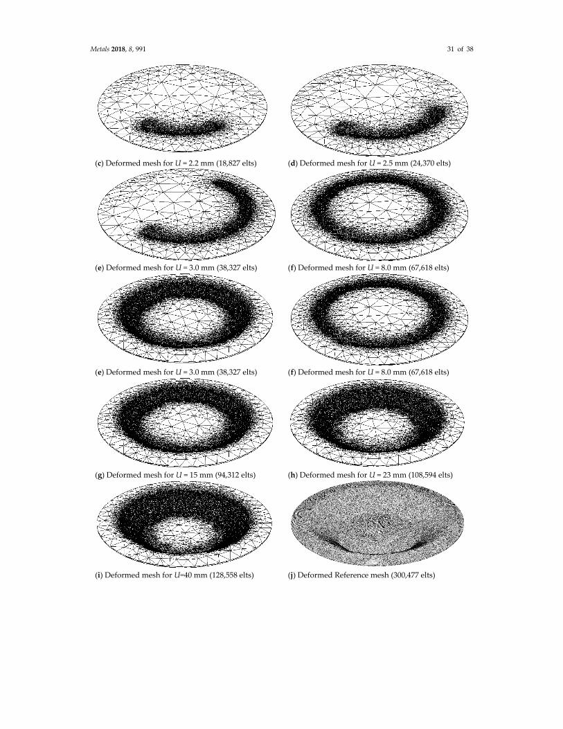
Metals 2018, 8, 991 31 of 38

(c) Deformed mesh for U = 2.2 mm (18,827 elts) (d) Deformed mesh for U = 2.5 mm (24,370 elts)

(e) Deformed mesh for U = 3.0 mm (38,327 elts) (f) Deformed mesh for U = 8.0 mm (67,618 elts)

(e) Deformed mesh for U = 3.0 mm (38,327 elts) (f) Deformed mesh for U = 8.0 mm (67,618 elts)

(g) Deformed mesh for U = 15 mm (94,312 elts) (h) Deformed mesh for U = 23 mm (108,594 elts)

(i) Deformed mesh for U=40 mm (128,558 elts) (j) Deformed Reference mesh (300,477 elts)

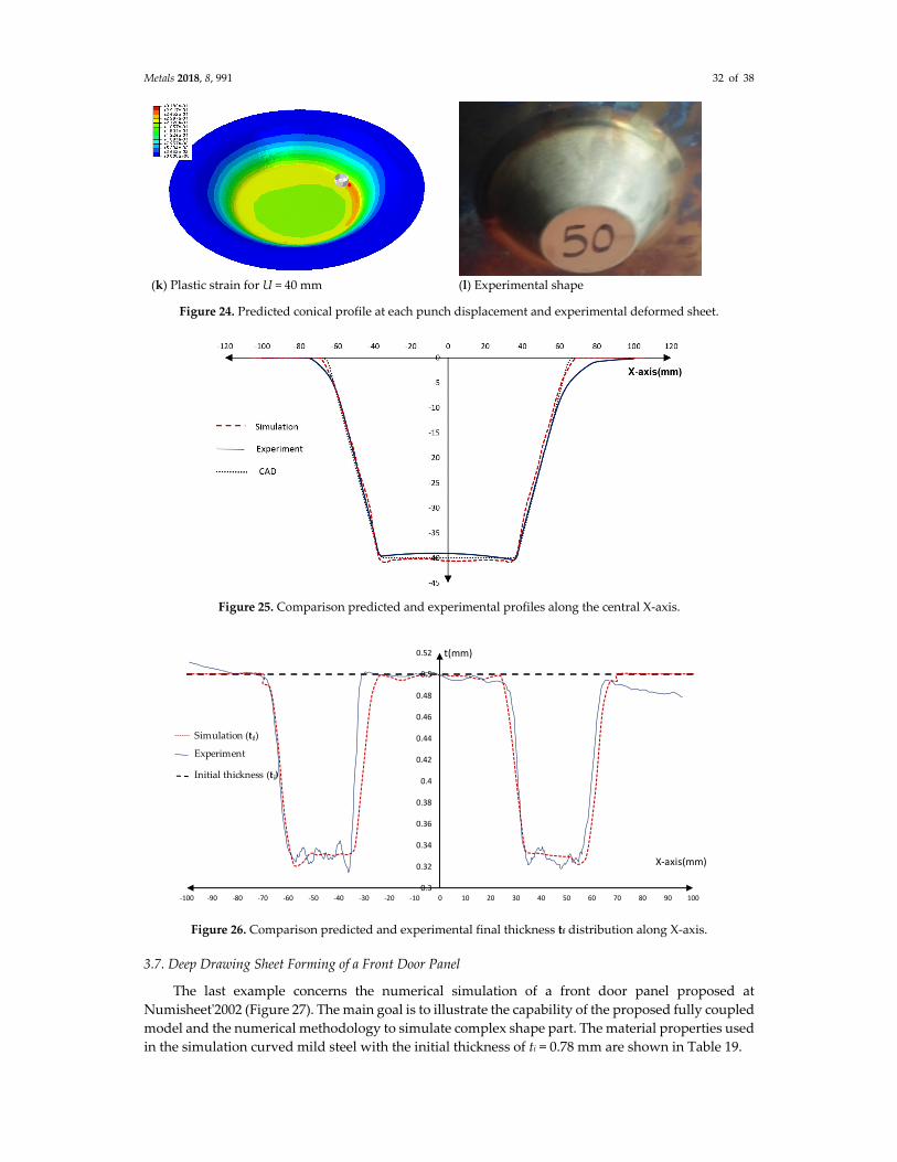
Metals 2018, 8, 991 32 of 38

(k) Plastic strain for U = 40 mm (l) Experimental shape

Figure 24. Predicted conical profile at each punch displacement and experimental deformed sheet.

Figure 25. Comparison predicted and experimental profiles along the central X-axis.

Figure 26. Comparison predicted and experimental final thickness tf distribution along X-axis.

3.7. Deep Drawing Sheet Forming of a Front Door Panel

The last example concerns the numerical simulation of a front door panel proposed at

Numisheet'2002 (Figure 27). The main goal is to illustrate the capability of the proposed fully coupled

model and the numerical methodology to simulate complex shape part. The material properties used

in the simulation curved mild steel with the initial thickness of ti = 0.78 mm are shown in Table 19.

0.3

0.32

0.34

0.36

0.38

0.4

0.42

0.44

0.46

0.48

0.5

0.52

-100 -90 -80 -70 -60 -50 -40 -30 -20 -10 0 10 20 30 40 50 60 70 80 90 100

X-axis(mm)

t(mm)

Experiment

Simulation (tf)

Initial thickness (ti)

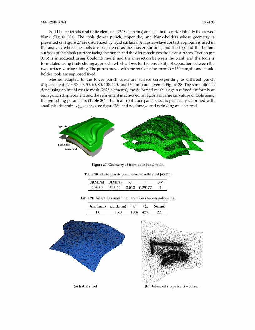
Metals 2018, 8, 991 33 of 38

Solid linear tetrahedral finite elements (2628 elements) are used to discretize initially the curved

blank (Figure 28a). The tools (lower punch, upper die, and blank-holder) whose geometry is

presented on Figure 27 are discretized by rigid surfaces. A master–slave contact approach is used in

the analysis where the tools are considered as the master surfaces, and the top and the bottom

surfaces of the blank (surface facing the punch and the die) constitutes the slave surfaces. Friction (=

0.15) is introduced using Coulomb model and the interaction between the blank and the tools is

formulated using finite sliding approach, which allows for the possibility of separation between the

two surfaces during sliding. The punch moves with the total displacement U = 130 mm, die and blank-

holder tools are supposed fixed.

Meshes adapted to the lower punch curvature surface corresponding to different punch

displacement (U = 30, 40, 50, 60, 80, 100, 120, and 130 mm) are given in Figure 28. The simulation is

done using an initial coarse mesh (2628 elements), the deformed mesh is again refined uniformly at

each punch displacement and the refinement is activated in regions of large curvature of tools using

the remeshing parameters (Table 20). The final front door panel sheet is plastically deformed with

small plastic strain pmax 15% (see figure 28j) and no damage and wrinkling are occurred.

Figure 27. Geometry of front door panel tools.

Table 19. Elasto-plastic parameters of mild steel [60,61].

A(MPa) B(MPa) C n -10ε ( ) s

203.39 645.24 0.010 0.25177 1

Table 20. Adaptive remeshing parameters for deep-drawing.

hmin(mm) hmax(mm) pc p

maxε δ(mm)

1.0 15.0 10% 42% 2.5

(a) Initial sheet (b) Deformed shape for U = 30 mm

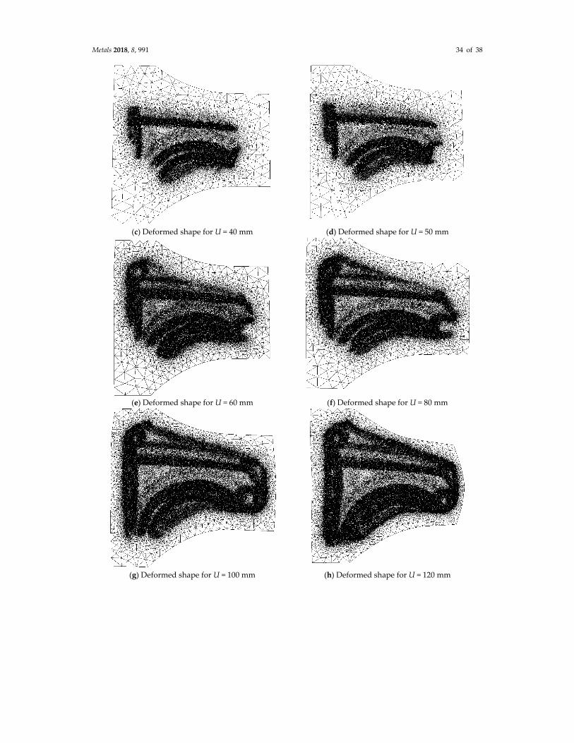
Metals 2018, 8, 991 34 of 38

(c) Deformed shape for U = 40 mm (d) Deformed shape for U = 50 mm

(e) Deformed shape for U = 60 mm (f) Deformed shape for U = 80 mm

(g) Deformed shape for U = 100 mm (h) Deformed shape for U = 120 mm

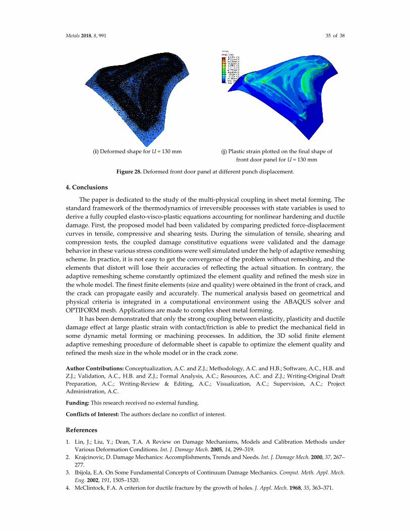
Metals 2018, 8, 991 35 of 38

(i) Deformed shape for U = 130 mm (j) Plastic strain plotted on the final shape of

front door panel for U = 130 mm

Figure 28. Deformed front door panel at different punch displacement.

4. Conclusions

The paper is dedicated to the study of the multi-physical coupling in sheet metal forming. The

standard framework of the thermodynamics of irreversible processes with state variables is used to

derive a fully coupled elasto-visco-plastic equations accounting for nonlinear hardening and ductile

damage. First, the proposed model had been validated by comparing predicted force-displacement

curves in tensile, compressive and shearing tests. During the simulation of tensile, shearing and

compression tests, the coupled damage constitutive equations were validated and the damage

behavior in these various stress conditions were well simulated under the help of adaptive remeshing

scheme. In practice, it is not easy to get the convergence of the problem without remeshing, and the

elements that distort will lose their accuracies of reflecting the actual situation. In contrary, the

adaptive remeshing scheme constantly optimized the element quality and refined the mesh size in

the whole model. The finest finite elements (size and quality) were obtained in the front of crack, and

the crack can propagate easily and accurately. The numerical analysis based on geometrical and

physical criteria is integrated in a computational environment using the ABAQUS solver and

OPTIFORM mesh. Applications are made to complex sheet metal forming.

It has been demonstrated that only the strong coupling between elasticity, plasticity and ductile

damage effect at large plastic strain with contact/friction is able to predict the mechanical field in

some dynamic metal forming or machining processes. In addition, the 3D solid finite element

adaptive remeshing procedure of deformable sheet is capable to optimize the element quality and

refined the mesh size in the whole model or in the crack zone.

Author Contributions: Conceptualization, A.C. and Z.J.; Methodology, A.C. and H.B.; Software, A.C., H.B. and

Z.J.; Validation, A.C., H.B. and Z.J.; Formal Analysis, A.C.; Resources, A.C. and Z.J.; Writing-Original Draft

Preparation, A.C.; Writing-Review & Editing, A.C.; Visualization, A.C.; Supervision, A.C.; Project

Administration, A.C.

Funding: This research received no external funding.

Conflicts of Interest: The authors declare no conflict of interest.

References

1. Lin, J.; Liu, Y.; Dean, T.A. A Review on Damage Mechanisms, Models and Calibration Methods under

Various Deformation Conditions. Int. J. Damage Mech. 2005, 14, 299–319.

2. Krajcinovic, D. Damage Mechanics: Accomplishments, Trends and Needs. Int. J. Damage Mech. 2000, 37, 267–

277.

3. Ibijola, E.A. On Some Fundamental Concepts of Continuum Damage Mechanics. Comput. Meth. Appl. Mech.

Eng. 2002, 191, 1505–1520.

4. McClintock, F.A. A criterion for ductile fracture by the growth of holes. J. Appl. Mech. 1968, 35, 363–371.

Metals 2018, 8, 991 36 of 38

5. Bonora, N.; Gentile, D.; Pirondi, A.; Newaz, G. Ductile damage evolution under triaxial state of stress: theory

and experiment. Int. J. Plast. 2005, 21, 981–1007.

6. Racy, J.R.; Tracy, D.M. On ductile enlargement of voids in triaxial stress fields. J. Mech. Phys. Solids 1969, 17,

201–217.

7. Gurson, A.L. Continuum theory of ductile rupture by void nucleation and growth and flow rules for porous

ductile media. J. Eng. Mater. Technol. 1997, 99, 2–15.

8. Needleman, A.; Tvergaard, V. An analysis of ductile rupture in notched bars. J. Mech. Phys. Solids 1984, 32,

461–490.

9. Tvergaard, V.; Niordoson, C. Non local plasticity effects on interaction of different size voids. Int. J. Plast.

2004, 20, 107–120.

10. Bonfoh, N.; Lipinski, P.; Carmasol, A.; Tiem, S. Micromechanical modeling of ductile damage of

polycrystalline material with heterogeneous particles. Int. J. Plast. 2004, 20, 85–106.

11. Kachanov, L.M. Introduction to Continuum Damage Mechanics. Martinus Nijhoff Publisher: Dordrecht, The

Netherlands, 1986.

12. Rabotnov, Y. Creep rupture. In Proceedings of the XII International Congress of Applied Mechanics,

Stanford, CA, USA, 26–31 August 1968; pp. 342–349.

13. Lemaitre, J. A continuous damage mechanics model for ductile fracture. J. Eng. Mater. Technol. 1985, 107, 83–

89.

14. Chaboche, J.L. On some modifications of kinematic hardening to improve the description of ratcheting

effects. Int. J. Plast. 1991, 7, 661–678.

15. Chaboche, J.L. Anisotropic creep damage in the framework of the continuum damage mechanics. Nucl. Eng.

Des. 1984, 79, 309–319.

16. Soyarslan, C.; Tekkaya, A.E. Finite deformation plasticity coupled with isotropic damage: Formulation in

principal axes and applications. Finite Elem. Anal. Des., 2010, 46, 668–683.

17. Bouchard, P.O.; Bourgeon, L; Fayolle, S.; Mocellin, K. An enhanced Lemaitre model formulation for materials

processing damage computation. Int. J. Mater. Form. 2011, 4, 299–315.

18. Brünig, M.; Chyra, O.; Albrecht, D.; Driemeier, L.; Alves, M. A ductile damage criterion at various stress

triaxialities. Int. J. Plast. 2008, 24, 1731–1755

19. Wang, T.J. A General Ductile Damage Model for Engineering Materials. In Fracture of Engineering Materials

and Structures; Teoh, S.H., Lee, K.H. Eds; Springer: Dordrecht, The Netherlands, 1991; pp. 798–803.

20. Peirs, J.; Verleysen, P.; Van Paepegem, W.; Degrieck, J. Determining the stress-strain behaviour at large

strains from high strain rate tensile and shear experiments. Int. J. Impact Eng. 2011, 38, 406–415.

21. Calamaz, M.; Coupard, D.; Girot, F. A new material model for 2D numerical simulation of serrated chip

formation when machining titanium alloy Ti-6Al-4V. Int. J. Mach. Tools Manuf. 2008, 48, 275–288.

22. Sun, Z.C.; Yang, H., Han, G.J.; Fan, X.G. A numerical model based on internal-state-variable method for the

microstructure evolution during hot-working process of TA15 titanium alloy. Mater. Sci. Eng. A 2010, 527,

3464–3471.

23. Zerilli, F.J. Dislocation mechanics–based constitutive equations. Metall. Mater. Trans. A 2004, 35, 2547–2555.

24. Zhang, H.; Wen, W.; Cui, H.; Xu, Y. A modified Zerilli–Armstrong model for alloy IC10 over a wide range

of temperatures and strain rates. Mater. Sci. Eng. A 2009, 527, 328–333.

25. Holmquist, T; Johnson, G. Determination of constants and comparison of results for various constitutive

models. J. Phys. IV 1991, 1, 853–860.

26. Hor, A.; Morel, F.; Lebrun, J.L; Germain, G. Modelling, identification and application of phenomenological

constitutive laws over a large strain rate and temperature range. Mech. Mater., 2013, 64, 91–110.

27. Johnson, G.R.; Cook, W.H. Fracture characteristics of three metals subjected to various strains, strain rates,

temperatures and pressure. Eng. Fract. Mech. 1985, 21, 31–48.

28. Cherouat, A.; Moreau, L.; Borouchaki, H. Advanced numerical simulation of metal forming processes using

adaptive remeshing procedure. Mater. Sci. Forum 2009, 614, 27–33.

29. Cherouat, A.; Borouchaki, H.; Saanouni, K.; Laug, P. Numerical methodology for metal forming processes

using elastoplastic model with damage occurrence. J. Mater. Sci. Technol. 2006, 22, 279–283.

30. Steinberg, D.J.; Cochran, S.G.; Guinan, M.W. A constitutive model for metals applicable at high-strain rate. J.

Appl. Phys. 1980, 51, 1498–1504, Doi:10.1063/1.327799.

31. Hoge, K.G.; Mukherjee, A.K. The temperature and strain rate dependence of the flow stress of tantalum. J.

Mater. Sci. 1977, 12, 1666–1672.

32. Zerilli, F.J.; Armstrong, R.W. Dislocation-mechanics-based constitutive relations for material dynamics

calculations. J. Appl. Phys. 1987, 61, 1816–1825.

33. Follansbee, P.S.; Kocks, U.F. A constitutive description of the deformation of copper based on the use of the

mechanical threshold. Acta Metall. 1988, 36, 81–93.

Metals 2018, 8, 991 37 of 38

34. Preston, D.L.; Tonks, D.L. Model of plastic deformation for extreme loading conditions. J. Appl. Phys. 2002,

93, 211–220; https://doi.org/10.1063/1.1524706.

35. Zhu, Y.Y.; Cescotto, S.; Habraken, A.M. A fully coupled elastoplastic damage modeling and fracture criteria

in metal forming processes. J. Mat. Proc. Tech. 1992, 32, 197–204.

36. Badreddine, H.; Labergère, C.; Saanouni, K. Ductile damage prediction in sheet and bulk metal forming. C.R.

Mec. 2016, 344, 296–318.

37. Chaboche, J.L.; Cailletaud, G. Integration methods for complex plastic constitutive equations. Comput. Meth.

Appl. Mech. Eng. 1996, 133, 125–155.

38. Kim, J.; Gao, X.; Srivatsan, T.S. Modeling of void growth in ductile solids: effects of stress triaxiality and

initial porosity. Eng. Fract. Mech. 2004, 71, 379–400.

39. Malcher, L.; Andrade Pires, F.M.; César de Sá, J.M.A. An assessment of isotropic constitutive models for

ductile fracture under high and low stress triaxiality. Int. J. Plast, 2012, 30-31, 81–115.

40. Xue, L.; Wierzbicki, T. Ductile fracture initiation and propagation modeling using damage plasticity theory.

Eng. Fract. Mech. 2008, 75, 3276–3293.

41. Lemaitre, J. Coupled elasto-plasticity and damage constitutive equations. Comput. Meth. Appl. Mech. Eng.

1985, 51, 31–49.

42. Boudifa, M.; Saanouni, K.; Chaboche, J.L. A micromechanical model for inelastic ductile damage prediction

in polycrystalline metals for metal forming. Int. J. Mech. Sci. 2009, 51, 453–464.

43. Simo, J.C.; Taylor R. Consistent tangent operators for rate independent elastoplasticity. Comput. Meth. Appl.

Mech. Eng. 1985, 48, 101-118.

44. Nagtegaal, J.C.; Taylor, L.M. Comparison of implicit and explicit finite element methods for analysis of sheet

forming processes. FE-Simulation of 3D Sheet Metal Forming Processes in Automotive Industry; VDI Verlag:

Dusseldorf, Germany, 1991.

45. Yang, D.Y.; Jung, D.W.; Song, Yoo, D.J.; Lee, J.H. Comparative investigation into implicit, explicit, and

iterative implicit/explicit schemes for the simulation of sheet-metal forming processes. J. Mater. Process.

Technol. 1995, 50, 39–53.

46. Chen, L. Comparisons of explicit and implicit finite element methods for sheet metal forming. Adv. Mater.

Res. 2014, 936, 1836–1839.

47. ABAQUS, version 6.14; Abaqus Inc.: Palo Alto, CA, USA, 2015.

48. Borouchaki, H.; Cherouat, A.; Laug, P.; Saanouni, K. Adaptive remeshing for ductile fracture prediction in

metal forming. C.R. Mec. 2002, 330, 709-716.

49. Borouchaki, H.; Grosges, T.; Barchiesi, D. Enhancement of the accuracy of numerical field computation using

an adaptive three-dimensional remeshing scheme. C.R. Mec. 2010, 338, 127–131.

50. Borouchaki, H.; Grosges, T.; Barchiesi, D. Improved 3d adaptive remeshing scheme applied in high

electromagnetic field gradient computation. Finite Elem. Anal. Des. 2010, 46, 84–95.

51. Borouchaki, H.; George, P.L.; Hecht, F.; Laug, P.; Saltel, E. Delaunay mesh generation governed by metric

specifications. Part I. Algorithms. Finite Elem. Anal. Des. 1997, 25, 61–83.

52. Borouchaki, H.; George, P.L.; Mohammadi, B. Delaunay mesh generation governed by metric specifications

Part II. Applications. Finite Elem. Anal. Des. 1997, 25, 85–109.

53. Broggiato, G.B.; Campana, F.; Cortese, L. Identification of Material Damage Model Parameters: an Inverse

Approach Using Digital Image Processing. Meccanica, 2007, 42, 9–17.

54. Springmann, M.; Kuna, M. Identification of material parameters of the Rousselier model by non-linear

optimization. Comput. Mater. Sci. 2003, 26, 202–209.

55. Yue, Z.M.; Soyarslan, C. ; Badreddine, H.; K Saanouni K.; Tekkaya, A.E. Identification of fully coupled

anisotropic plasticity and damage constitutive equations using a hybrid experimental–numerical

methodology with various triaxialities. Int. J. Damage Mech. 2015, 24, 683–710.

56. Feng, F.; Li, J.; Yuan, P.; Zhang, Q.; Huang, P.; Su, H.; Chen, R. Application of a GTN damage model

predicting the fracture of 5052-O aluminum alloy high-speed electromagnetic impaction. Metals 2018, 8, 761.

doi:10.3390/met8100761

57. Zhang, J.; Cherouat, A.; Borouchaki, H. 3D Thermo-Mechanical Simulation Coupled with Adaptive

Remeshing for Metal Milling. Adv. Mater. Res. 2013, 698, 11–20

58. Abedini, A.; Butcher, C.; Worswick, M. J. Fracture characterization of rolled sheet alloys in shear loading:

studies of specimen geometry, anisotropy, and rate sensitivity. Exp. Mech. 2017, 57–75.

doi.org/10.1007/s11340-016-0211-9

59. Zhang, J. Multi-axial Damage Model for Numerical Simulation of Metal Forming Processes Using 3D

Adaptive Remeshing Procedure. PhD Thesis, University of Technology of Troyes, Troyes, France, April 2005.

60. Husson, C.; Correia, J.P.M.; Daridon, L.; Ahzi, S. Finite elements simulation of thin copper sheets blanking:

Study of blanking parameters on sheared edge quality. J. Mater. Process. Technol. 2008, 199, 74–83.

Metals 2018, 8, 991 38 of 38

61. Cherouat A.; Ma X.; Borouchaki H.; Zhang Q. Numerical study of Multi-Point Forming of thick sheet using

remeshing procedure. In proceeding of ESAFORM 2018, Palermo, Italy, 23–25 April 2018.

62. Saidi, B.; Giraud-Moreau, L.; Cherouat, A. Optimization of the Single Point Incremental Forming Process for

titanium sheets by using response surface. MATEC Web Conf. 2016, 80, 10011, doi:

10.1051/matecconf/20168010011.

63. Sena, J.I.V.; Alves de Sousa, R.J; Valente, R.A.F. Single point incremental forming simulation with an

enhanced assumed strain solid-shell finite element formulation. Int. J. Mater. Form. 2010, 3, 963–966.

64. Liu, Z.; Daniel, W.J.T.; Li, Y. Multi-pass deformation design for incremental sheet forming: Analytical

modeling, finite element analysis and experimental validation. J. Mater. Process. Technol. 2014, 214, 620–634,

doi: 10.1016/j.jmatprotec.2013.11.010.

65. Honarpisheh, M.; Jobedar, M.; Alinaghian, I. Multi-response optimization on single-point incremental

forming of hyperbolic shape Al-1050/Cu bimetal using response surface methodology. Int. J. Adv. Manuf.

Technol. 2018, 96, 3069–3080, doi: 10.1007/s00170-018-1812-5.

66. Duflou, J.; Tunçkol, Y.; Szekeres, A.; Vanherck, P. Experimental study on force measurements for single point

incremental forming. J. Mater. Process. Technol. 2007, 189, 65–72. doi: 10.1016/j.jmatprotec.2007.01.005

67. Li, Y.; Chen, X.; Liu, Z. A review on the recent development of incremental sheet-forming process. Int. J. Adv.

Manuf. Technol. 2017, 92, 2439–2462. doi: 10.1007/s00170-017-0251-z

68. Ambrogio, G.; De Napoli, L.; Filice, L. Application of Incremental Forming process for high-customized

medical product manufacturing. J. Mater. Process. Technol. 2005, 162, 156–162. doi:

10.1016/j.jmatprotec.2005.02.148

© 2018 by the authors. Licensee MDPI, Basel, Switzerland. This article is an open access

article distributed under the terms and conditions of the Creative Commons Attribution (CC

BY) license (http://creativecommons.org/licenses/by/4.0/).