Simulation of parapet walls' benefits in local area of U-Minh qua Du an... · structures are parapet walls using various types of materials and structures that have been constructed

LMDCZ project: Shoreline protection measures (WP6)

1

Simulation of parapet walls' benefits in local area of U-Minh

1. Introduction

Coastal monitoring data for U Minh reveals that erosion has increased in recent years. To mitigate this negative

impact, many of the construction measures have been developed by the local authorities. Among these types of

structures are parapet walls using various types of materials and structures that have been constructed along the

shore. Monitoring data on the effect of these types of structures have been reported in recent years, which show

that successes and failures are different from place to place depending on the location of the building. This study

aims to simulate the effect of hardened parapet walls on the coast protection of the U Minh.

Figure 1: A typical form of parapet walls for coast protection

In order to study this erosion process, various numerical models are used simultaneously including Telemac2D

(hydrodynamic), Tomawac (wave) and Sisyphe (sediment transport). The detailed computing mesh including

parapet wall structure will focus on the zone from the Bay-Hap to Ong Doc River.


2

2. Study area and boundary conditions

The local area of interest is the western coastal area of the Mekong Delta, which is confined to the south, abutting

the Gulf of Thailand. The average width is 40 km from the coast and 126 km from Ca Mau Cape to the north. This

study area is characterized by 87 thousand unstructured triangle elements of which the largest mesh is up to

2000m (offshore elements) and the smallest is 8m (or 3m in case of built-in wavefronts) for the coastal zone. The

wall location is approximately 400m from the shore, extends L = 7000m and has a crest elevation above the highest

water level in the area. The walls are installed almost parallel to the shore.

Figure 2.1a: Local study area


3

Figure 2.1b: Simulation of parapet walls in study area

Figure 2.2: Boundary conditions


4

Tidal: The open boundary at offshore is determined from astronomical tide extracted from TPXO database during

the study period.

Figure 2.3: Tidal boundary at typical positions A1 and A2 during Aug. & Sep 2016

Wave: At the open boundary, wave data is determined from a global database of wind and wave effects on the

surface domain determined from NOAA for the boundary conditions of the Tomawac model.

Figure 2.4a: Wave height HM0 from NOAA at coordinates (334682.9 ; 884599.1)

0

0.5

1

1.5

2

2.5

0 96 192 288 384 480 576 672 768 864 96010561152124813441440

HM

0 (

m)

T (h)

Feb. & Mar. 2016

Aug. & Sep. 2016


5

Figure 2.4b: Wave height HM0 from NOAA at coordinates (335343.7 ; 1050487.3)

Figure 2.4c: Wave height HM0 from NOAA at position A1 of coordinates (439869.6 ; 954419.1)

0

0.2

0.4

0.6

0.8

1

1.2

1.4

0 96 192 288 384 480 576 672 768 864 96010561152124813441440

HM

0 (

m)

T (h)

Feb. & Mar. 2016Aug. & Sep. 2016

0

0.5

1

1.5

2

0 96 192 288 384 480 576 672 768 864 96010561152124813441440

HM

0 (

m)

T (h)

Feb .& Mar. 2016

Aug. & Sep. 2016


6

Figure 2.5: Typical wind rose in U-Minh coast in: (a) 8-9 /2016 and (b) 2-3/2016

The results from the wind rose show that these are two distinctly monsoonal periods. In the months of January &

February, the winds are relatively intense compared to August and September. Wind direction in January &

February is mainly from the East, while in August and September; it is mainly in the west and southwest.

Discharge: Discharge in Ong-Doc river are taken as follow:

(a) (b)


7

Figure 2.6: Discharge in Aug 2016 at Ong-Doc river

Sediment

Simulation of sediment transport in the area is considered as non-cohesive transport. The distribution of sand is

assumed to be uniform throughout the study area. From the monitoring data of granular, the particle size is divided

into four representative sizes: 0.06mm, 0.125mm, 1.0 mm, 1.5mm; with the initial rates of 40%, 30%, 20% and 10%.

The boundary conditions are:

- The open offshore boundary is free and balance condition.

- In the upstream areas, the boundary conditions are specified of Direclet type with the monitoring level.

The main parameters of simulation are as follows:

- The law of friction according to Nicuradse

- The bottom sediment transport model according to Soulsby - Van Rijn

- The settling velocity is determined by the Van Rijn, depending on the characteristic of the sediment layer.

- The value of the Shield taken by the Rijn Valves depends on the dimensionless dimension of the sediment

classe.

3. Simulation results

Simulations are made for two representative seasons: the southwest monsoon season and the northeast monsoon

season. Each simulation season lasts for 2 months:

- West-South monsoon season: 8-9 / 2016

- East - North monsoon season: 2-3 / 2016

-80

-60

-40

-20

0

20

40

60

80

0 72 144 216 288 360 432 504 576 648 720

Q (

m3/s

)

T (h)


8

a. Hydrodynamic

The results show that the flow tends to go from Ca-Mau cap to the north. Simulation results for the local area

indicate a trend of mainstream going from the East Sea to the West Sea.

Figure 3.1: Field of average velocity in 8-9/2016 at coast.

(a) without parapet; (b) with parapet.

[a] [b]


9

Figure 3.2: Field of instantenous velocity at typical coastal position.

(a) at 10h, 17/9/2016; (b) at 18h, 17/9/2016.

Figure 3.3: Distribution of flow velocity in 8-9/2016 at typical coastal position [1].

(a) (b)


10

Comments on field of average velocity are as follow:

- The average field velocity in both cases with walls and without walls did not change much in the area

outside the wall (Figure 3.1).

- The instantaneous velocity field in the domain varies in two main directions, North and South, which are

closely related to tidal fluctuations in the region (Figure 3.2).

- With the presence of walls, the coastal flow almost disappeared inside of the wall. The main flows in the

coast follow the north and south direction (Figure 3.3). This result does not change with and without walls.

b. Waves

Waves in the local model are described from boundary conditions in the West Sea extracted from the NOAA global

wave data. In addition, the waves are also created by the effects of the wind on the surface of the domain. Wind

data is also collected from NOAA. In this model, these wave and wind data are changed over time and space.

Figure 3.4: Instantenous wave height HM0 (m): (a) at 12h, 19/9/2016; (b) at 12h, 21/9/2016

(a) (b)

(a) (b)


11

Figure 3.5: Average wave height HM0 (m) in 8-9/2016

Figure 3.6: Variation of average wave height HM0 (m) in 8-9/2016 at sections 1-1 & 2-2


12

Figure 3.7: Variation of wave height HM0(t) over time at typical positions [1] in two cases: with (continous red line)

and without (dashed blue lines) walls.

Some general comments about waves in the domain area are as follows:

- With the construction of wall structures with crest above the sea level, the effect of blocking waves

approaching the coastal area is radical. The erosion phenomenon due to this factor is therefore also

excluded (Figure 3.4).

- The wave reduction effect of parapet is described in Fig. 3.6. The waves are almost eliminated behind the

wall.

- Waves at the front of the wall are almost unchanged in case with and without walls (position [1] in Figure

3.7).

c. Sediment transport

The results of sediment transport are determined from the combination of three equations, including

hydrodynamics, waves, and morphological change. The sediment boundary at the sea is considered as a free zone

for the movement of bed load and suspended sediment. Due to the limit of field data (bathymetry and sediments),

this model only considers the confluences Bay Hap and Ong Doc. Concentration of suspended sediment is set at 150

mg / l.

Under the influence of the hydrological regime and U Minh coastal shores, satellite data for suspended sediments

for the month were recorded as follows:


13

Figure 3.8: The typical average concentration of suspended sediment in August and February 2016

from the satellite data

The above graph shows the effect of coastal waves on the concentration of suspended sediment in the area. The

following charts and graphs summarize the simulation results of sediment transport in the area.


14

Figure 3.9: Average suspended sand concentration in 8-9/2016 : (a) without walls; (b) with walls

Figure 3.10: Instantenous suspended sand concentration over time at position [1], behind walls

(a): without walls (dashed red lines); (b) with walls (continous blue line).

0

0.05

0.1

0.15

0.2

0.25

0.3

0.35

0 96 192 288 384 480 576 672 768 864 960

SS

C (

g/l

)

T (h)

Without parapet With parapet

(a) (b)


15

Figure 3.11: Average suspended sand concentration over time at position [2], in front of walls

(a): without walls (dashed red lines); (b) with walls (continous blue line).

Comparing the results from the graphs gives the following conclusions:

- Coastal waves greatly affect the concentration of suspended sediment. This result was recorded from

satellite imagery data and was explained by physical phenomena in which coastal breaking waves increase

the concentration of suspended sediment under the effect of high intensity turbulent flows in this area.

- One can observe clearly that the parapet wall reduces the concentration of sediment, especially behind the

wall, within the wall construction. In Figure 3.10, almost all of the shoreline is protected by parapet wall

with a lower average sediment concentration than in other locations. This result may explain the wave

attenuate effect and thus reduce the turbidity in this area.

- Figure 3.11 also shows that the suspended sediment concentration at a typical location in front of the wall

in case of with and without walls does not change much comparing to back wall.

0.15

0.19

0.23

0.27

0.31

0.35

0.39

0 96 192 288 384 480 576 672 768 864 960

SS

C (

g/l

)

T (h)

Without parapet With parapet


16

Figure 3.12: Average sediment fluxes in 8-9/2016: (a) without walls; (b) with walls

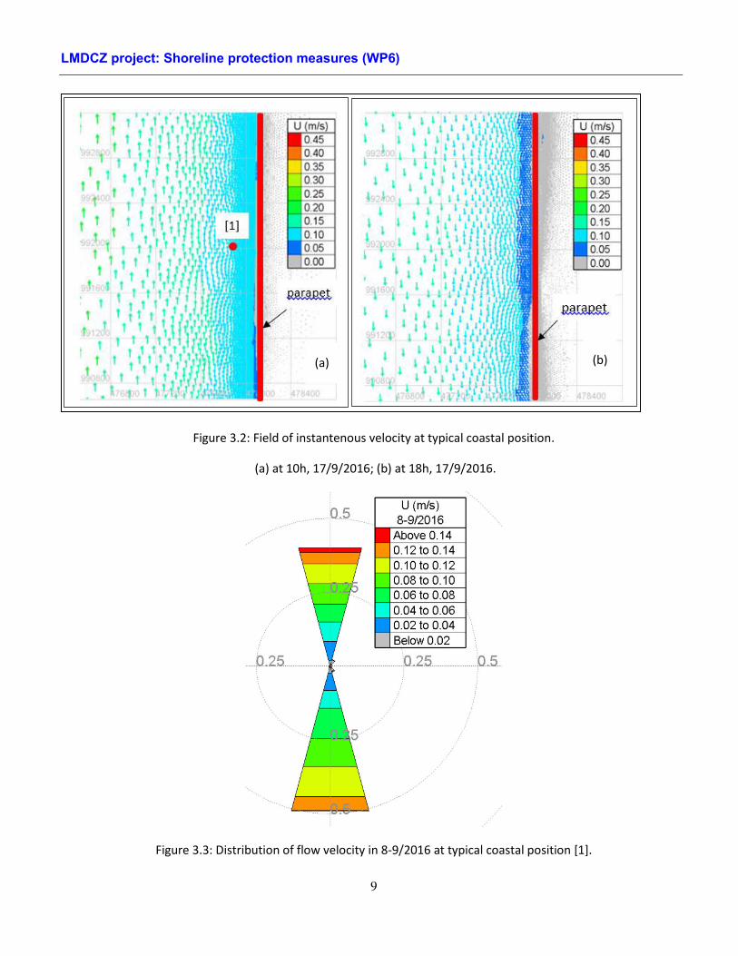
In order to quantify the sediment transport within the wall construction area, the sediment budget analysis in the

front and behind walls will be conducted. The sediment budget analysis in typical area of B=800m in width and

L=7000m in length will be conducted (see Figure 3.13).

(a) (b)


17

Figure 3.13: Area for sediment budget analysis


18

Figure 3.14: Erosion/accretion after 2 months: (a) 8-9/2016; (b) 2-3/2016

Table 3.1: Sediment budget analysis for zone A behind parapet

In (m3) Out (m

3) (In-Out), m

3 Comments

Tháng 8-9/2016 40.9 15.4 25.5 (+) accretion

Tháng 2-3/2016 149.5 20.1 129.4 (-) erosion

The following results compare the erosion rate in the zone behind the wall to the shore (Area A, Fig. 3.13) for two

cases with and without walls.

Table 3.2: Sediment budget analysis for coastal area in 8-9/2016

Case In (m3) Out (m

3) (In-Out), m

3 Comments

without parapet 94.1 242.3 -148.2 (+) accretion

with parapet 40.9 15.4 25.5 (-) erosion

(a) (b)


19

Table 3.3: Sediment budget analysis for coastal area in 2-3/2016

Case In (m3) Out (m

3) (In-Out), m

3 Comments

without parapet 302.7 375.6 -72.9 (+) accretion

with parapet 149.5 20.1 129.4 (-) erosion

Comment:

- The erosion in the foot of wall might occur which can be explained by the phenomenon of breaking waves

moving to shore and exposing to the wall. A small accretion to the area behind the wall is also noted.

- The wall has positive effect for the accretion of the area behind the wall. This result can be explained by the

"absolute" wave breaking effect of the wall for the beach.

4. Simulation results with the T-groyne protection

This section presents the results of protection using T-shaped groynes along the coast. Unlike the wall structure

mentioned in the previous section, the structure considered in this section consists of successive T-shaped groynes,

as described by the following diagram.

Figure 4.1: Location and size of the T-groyne


20

Relative position and typical groyne size are as follows:

- Width of groyne’s wing Ls = 600 m

- Clearance between wings Lg = 50 m

- Height of groyne (from wings) Lb = 400 m

a. Results of wave simulation

Waves spreading to the shore will encounter the groynes. The wave attenuation of the T-groyne is shown in the

following graphs.

Figure 4.2a: Average wave height HM0 in 8-9/2016 between the T-groynes


21

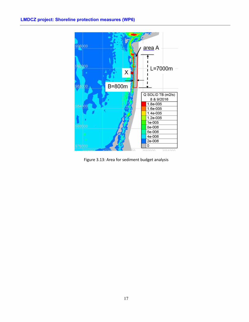
Figure 4.2b: Average wave height HM0 in 2-3/2016 between the T-groynes


22

Figure 4.3: Average wave height HM0 in 8-9/2016 at section 1-1




23


The results from the above graphs give the following remarks:

- The waves propagating to the T-groyne are almost blocked on the width of Ls.

- In the space between two trenches (Lg gap), waves can still propagate to shore. However, the wave

intensity is smaller than in the case of no groyne (see section 1-1).

- The wave passing through the gap between the two groynes has horizontal diffusion (see section 2-2).

b. Simulation results of sediment transport

The following results compare the erosion rates from continuous parapet and T-shaped groynes.

Table 4.1: Sediment budget analysis of coastal area in 8-9/2016

Case In (m3) Out (m

3) (In - Out), m

3 Comment

Continuous parapet 40.9 15.4 25.5 (+) accretion

T-groyne 7714.2 918.5 6795.7 (-) erosion

Table 4.2: Sediment budget analysis of coastal area in 2-3/2016

Case In (m3) Out (m

3) (In - Out), m

3 Comment

Continuous parapet 149.5 20.1 129.4 (+) accretion

T-groyne 2754.6 369.3 2385.3 (-) erosion


24

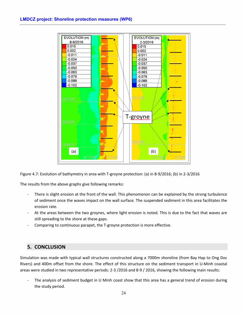
Figure 4.7: Evolution of bathymetry in area with T-groyne protection: (a) in 8-9/2016; (b) in 2-3/2016

The results from the above graphs give following remarks:

- There is slight erosion at the front of the wall. This phenomenon can be explained by the strong turbulence

of sediment once the waves impact on the wall surface. The suspended sediment in this area facilitates the

erosion rate.

- At the areas between the two groynes, where light erosion is noted. This is due to the fact that waves are

still spreading to the shore at these gaps.

- Comparing to continuous parapet, the T-groyne protection is more effective.

5. CONCLUSION

Simulation was made with typical wall structures constructed along a 7000m shoreline (from Bay Hap to Ong Doc

Rivers) and 400m offset from the shore. The effect of this structure on the sediment transport in U-Minh coastal

areas were studied in two representative periods: 2-3 /2016 and 8-9 / 2016, showing the following main results:

- The analysis of sediment budget in U Minh coast show that this area has a general trend of erosion during

the study period.


25

- Breaking waves near the coast have a clear effect on the sediment concentration in coastal areas. This is

consistent with the data observed by satellites over time.

- The parapet walls attenuate the wave for the coastal area behind the wall.

- The wall structure reduces the concentration of suspended sediment in the construction area.

- The continuous parapet has almost no effect on instantaneous flow as well as average flow. This can be

explained by the fact that its direction is almost the same as the velocity fields.

- The results of sediment budget analysis within the construction areas of walls (in the section of Song Hap

river to Ong Doc river) shows that the structure of the wall parallel to the shore reduces erosion in the area

behind the wall. This means that the corresponding coastal zone is protected. This is a clear positive impact

for this type of construction.

- Erosion at the foot of wall may occur due to the effect of breaking waves when exposed to the wall (Figure

4.7).

- T-groyne measure demonstrate the ability of coastal sediment trapping is quite good comparing to other

measures.


26

REFERENCES

EDF R&D. Guide to programming in the Telemac system

EDF R&D . Sisyphe v6.3 User's Manual

EDF R&D. TOMAWAC software for sea state modelling on unstructured grids over oceans and coastal

seas. Release 6.1

HERVOUETJean Michel (2007). Hydrodynamics of Free Surface Flows modelling with the finite

element method. WILEY.

LANG Pierre et all (2010).Telemac2d_manuel_utilisateur_v6p0. EDF.

MEISSNER Loren P. (1995). Fortran 90. PWS Publishing Company.

NOAA. National Geophysical Center. http://www.ngdc.noaa.gov/mgg/global/global.html.

OTIS Regional Tidal Solutions. http://volkov.oce.orst.edu/tides/region.html.

PH M Văn Hu n(2002). Động lực học Biển-Phần 3: Thủy triều. Đ i Học Quốc Gia Hà Nội.

TR N Thục et all. (2012). Tác động của nước biển dâng đến chế độ thủy triều dọc bờ biển Việt Nam.

T p chí Khoa học và Công nghệ Biển số 1-2012.

http://www.ngdc.noaa.gov/mgg/global/global.html

http://volkov.oce.orst.edu/tides/region.html

http://volkov.oce.orst.edu/tides/region.html

Simulation of parapet walls' benefits in local area of U-Minh qua Du an... · structures are parapet walls using various types of materials and structures that have been constructed

Documents