Simulation of High Reynolds Number Vascular Flowsfischer/pubhtml/high_re.pdfSimulation of High Reynolds Number Vascular Flows Paul F. Fischer,a Francis Loth,b Seung E. Lee,c Sang-Wook

Simulation of High Reynolds Number Vascular Flows

Paul F. Fischer,a Francis Loth,b Seung E. Lee,c Sang-Wook Lee,d David S. Smith,b andHisham S. Bassiounye

aMathematics and Computer Science Division, Argonne National LaboratoryArgonne, IL 60439, U.S.A.

bDept. of Mechanical Engineering, University of Illinois,Chicago, IL 60607, U.S.A.

cDept. of Mechanical Engineering, Massachusetts Institute of Technology,Cambridge, MA

dImaging Research Laboratories, Robarts Research Institute,London, ON N6A 5K8, Canada

eSection of Vascular Surgery, University of Chicago,Chicago, IL 60607, U.S.A.

1. Introduction

While much of the hemodynamics in a healthy human body has low Reynolds number,resulting in laminar flow, relatively high Reynolds number flow is observed at some spe-cific locations, which can cause transition to turbulence. (The term “turbulence” refersto the motion of a fluid having local velocities and pressures that fluctuate randomly.)For example, the peak Reynolds number in the human aorta has been measured to beapproximately 4000 [25]. Surgical constructions such as the arteriovenous (AV) graft,which consists of a prosthetic graft material surgically attached between an artery and avein, also results in relatively high Reynolds number flow (1000–3000) [8,40]. Complexgeometries such as a severe stenosis also can cause turbulent flow in the vasculature [22].

The simulation of turbulent vascular flows presents significant numerical challenges.Because such flows are only weakly turbulent, they lack an inertial subrange that isamenable to subgrid-scale modeling required for large-eddy or Reynolds-averaged Navier-Stokes simulations. The only reliable simulation approach at present is to directly resolveall scales of motion. While the Reynolds number is not high (Re=1000–2000, typ.),the physical dissipation is nonetheless small, and high-order methods are essential forefficiency. Moreover, turbulent blood flow exhibits a much broader range of scales thandoes its laminar (healthy) counterpart and thus requires an order of magnitude increasein spatial and temporal resolution. For example, recent work by Sherwin and Blackburnhas shown that roughly one to two million gridpoints are required for spectral/spectral-element-based simulations of turbulence in an idealized stenosis [42].

1

2 P. Fischer et al.

In this paper, we discuss temporal and spatial resolution requirements for direct nu-merical simulation in two cases where turbulence is commonly found in the vasculature,namely, in a stenosed carotid artery and in the venous anastomosis of an arteriovenousgraft. We also describe recent developments in the spectral element method designedspecifically for the simulation of high-Reynolds number vascular flows. The paper is orga-nized as follows. Section 2 presents an outline of the spectral element method, including adiscussion of the transport properties relevant to high-Reynolds number flow simulation.Section 3 discusses the imposition of flow division and treatment of outflow boundaryconditions for turbulent flows. Section 4 briefly describes our mesh generation procedure.Section 5 presents the results of grid convergence studies for two turbulent flow cases,including experimental validation results. Section 6 closes with a brief summary.

2. Navier-Stokes Discretization

We consider numerical solution of incompressible Navier-Stokes equations in Ω,

∂u

∂t+ u · ∇u = −∇p +

1

Re∇2u, ∇ · u = 0, (1)

subject to appropriate initial and boundary conditions. Here, u is the velocity field, p isthe pressure normalized by the density, and Re = UD/ν is the Reynolds number basedon the characteristic velocity U , length scale D, and kinematic viscosity ν. For bloodflow, the Newtonian assumption is valid for shear rates approximately 100 s−1 and above,which generally holds in larger vessels where transition is expected to take place. The useof a rigid domain follows current practice in the field, and its validity varies from vesselto vessel. For example, in arteriovenous grafts, wall motion is on the order of 1 percent ofthe vessel diameter [32], so a rigid assumption is a reasonable starting point for analysis ofthe flow transition process. Such an assumption, however, precludes incorporation of anyenergy storage and exchange mechanism between the flowing blood and the elastic wall.While we anticipate studying such phenomena in the near future, our focus here is onthe numerical algorithms related to (1). Our discretization of (1) is based on the spectralelement method (SEM) which is described in detail elsewhere (e.g.,[6,9,10]). Here, we givea brief outline of the SEM and numerical timestepping scheme to provide a context forthe features that are specific to the simulation of high-Reynolds number vascular flows.

For the temporal discretization, we employ a semi-implicit formulation in which thenonlinear terms are treated explicitly and the remaining linear Stokes problem is treatedimplicitly. The time derivative in (1) is approximated by using a kth-order backwardsdifference formula (BDFk, k=2 or 3), which for k=2 reads

3un − 4un−1 + un−2

2∆t= S(un) + NLn. (2)

Here, un−q represents the velocity at time tn−q, q = 0, . . . , 2, and S(un) is the linear sym-metric Stokes operator that implicitly incorporates the divergence-free constraint. Theterm NLn approximates the nonlinear terms at time level tn and is given by the extrap-olant NLn := −

∑j αju

n−j · ∇un−j. For k = 2, the standard extrapolation would useα1 = 2 and α2 = −1. Typically, however, we use a three-term second-order formulationwith α1 = 8/3, α2 = −7/3, and α3 = 2/3, which has a stability region that encompasses a

High Reynolds Number Vascular Flows 3

part of the imaginary axis, similar to third-order Adams-Bashforth [20]. As an alternativeto (2), we frequently use the operator-integration-factor scheme of Maday et al. [35] thatcircumvents the CFL (Courant-Friedrichs-Lewy) stability constraints by setting NLn = 0and replacing the left-hand side of (2) with an approximation to the material derivativeof u. In either case, one obtains an unsteady Stokes problem of the form

Hun − ∇pn = fn

∇ · un = 0,(3)

to be solved implicitly. For k = 2, H is the Helmholtz operator H :=(

32∆t

− 1Re∇2

). In

Section 3, we will formally refer to (3) in operator form Sus(un) = fn. In concluding

our temporal discretization overview, we note that we often stabilize high-Re cases byfiltering the velocity at each step (un = F (un)), using the high-order filter described in[10,13].

Spatial discretization of (3) is based on the lPN − lPN−2 spectral element method ofMaday and Patera [34]. The SEM is a high-order weighted residual approach similar tothe finite element method (FEM). In the SEM, functions are approximated as tensor-product Lagrange polynomials of degree N on each of E subdomains (elements), Ωe,e = 1, . . . , E, leading to n ≈ ENd unknown basis coefficients for each velocity componentin lRd, d=1 or 2, with N=4–16 being typical. In the lPN − lPN−2 method, the pressureis approximated as a tensor-product polynomial of degree N − 2 and is discontinuous,leading to np = E(N − 1)d basis coefficients for p.

The relatively high polynomial degree of the SEM is enabled by the use of tensor-product bases having the form (in 2D)

u(xe(r, s))|Ωe =N∑

i=0

N∑

j=0

ueijh

Ni (r)hN

j (s) , (4)

where the ueijs are the nodal basis coefficients on element Ωe and hN

i ∈ lPN is the La-grange polynomial based on the Gauss-Lobatto quadrature points, ξN

j Nj=0 (the zeros of

(1 − ξ2)L′

N(ξ), where LN is the Legendre polynomial of degree N). Here xe(r, s) is thecoordinate mapping from Ω = [−1, 1]d to Ωe, implying that the elements are curvilinearquadrilaterals in 2D or hexahedra in 3D.

In the SEM, all of the operator evaluations for explicit timestepping and iterativesolution of implicit substeps are performed in matrix-free form. As first suggested byOrszag [38], this approach leads to a reduction in memory and operation counts fromO(EN6) (in 3D) to O(EN3) and O(EN4), respectively. Unstructured data accesses arerequired at the global level (i.e., for e = 1, ..., E), but local data accesses within Ωe

are structured in i-j-k form. In particular, differentiation—a central kernel in operatorevaluation—can be implemented as a cache-efficient matrix-matrix product. For example,ue

r,ij =∑

p Dipuepj, with Dip := h′

p(ξi) would return the derivative of (4) with respect tothe computational coordinate r at the points (ξi, ξj). Differentiation with respect to x isobtained by the chain rule [6].

Inserting the SEM basis (4) into the weak form of (3) and applying numerical quadra-ture, we obtain the discrete unsteady Stokes system

H un − DT pn = B fn, D un = 0. (5)

4 P. Fischer et al.

Here, H = 1Re

A+ 32∆t

B is the discrete equivalent of H; −A is the discrete Laplacian, B isthe (diagonal) mass matrix associated with the velocity mesh, D is the discrete divergenceoperator, and fn accounts for the explicit treatment of the nonlinear terms. Note thatthe Galerkin approach implies that the governing system in (5) is symmetric and that thematrices H, A, and B are all symmetric positive definite.

The Stokes system (5) is solved approximately, by using the kth-order operator splittinganalyzed in [3,35,39]. The splitting is applied to the discretized system so that ad hocboundary conditions are avoided. For k = 2, one first solves

H u = B fn + DT pn−1, (6)

which is followed by a pressure correction step

Eδp = −Du, un = u + ∆tB−1DT δp, pn = pn−1 + δp, (7)

where E := 23∆tDB−1DT is the Stokes Schur complement governing the pressure in

the absence of the viscous term. Substeps (6) and (7) are solved with preconditionedconjugate gradient (PCG) iteration. Jacobi preconditioning is sufficient for (6) becauseH is strongly diagonally dominant. E is less well-conditioned and is solved either by themultilevel overlapping Schwarz method developed in [9,12] or by more recent Schwarz-multigrid methods [11,33]. The solution of (7) constitutes the most compute-intensivesubstep of our Navier-Stokes time advancement.

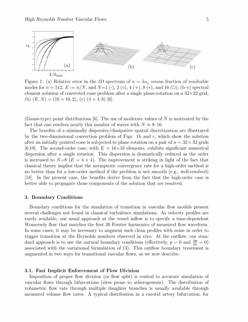
Convergence PropertiesThe primary distinction of the SEM is that it is designed for much higher approximation

orders than are typically used with the FEM. With the SEM, orders N=4–16 are typical(and feasible, because of the use of matrix-free operator evaluation [6]). These high orderslead to excellent transport (minimal numerical diffusion and dispersion) for a significantlylarger fraction of the resolved modes than is possible with the FEM. This point is illus-trated in Fig. 1, which shows the error, εk, for eigenvalues associated with the modelconvection problem ut +ux = 0 on [0, 2π] versus the fraction of resolvable modes, k/kmax.Here kmax = n/2, according to the Nyquist criterion, n = EN is the number of degrees offreedom for this one-dimensional problem, and εk := |k − k|/k,. The approximate eigen-value is computed as k := (φ′

k, Dφk)N/(φ′

k, φ′

k)N ,where φk(x) := cos(kx), D is the spectralelement derivative operator associated with E uniformly sized elements of order N , and(., .)N refers to quadrature on the N +1 Gauss-Lobatto Legendre nodal points within eachdomain that also correspond to the Lagrange interpolation points. Figure 1a shows theerrors for n=512, N=1, 2, 4, 8, 16, and E := n/N . Taking 1 percent as an acceptableerror threshold (indicated by the dashed line in Fig. 1a), we see that 10 percent of themodes are well resolved with linear elements (N=1), whereas approximately half of themodes are well resolved for N ≥ 8. Thus, the SEM provides roughly a fivefold reductionin the required number of gridpoints per space dimension to properly propagate wavesat typical engineering tolerances. Note that, because the abscissa is scaled by kmax, thecurves in Fig. 1a exhibit little material change with increased resolution; as n increases,one resolves more waves, but the relative fraction remains unchanged. By the same token,one cannot circumvent the Nyquist sampling criterion by simply increasing N . In fact,as N −→ ∞, one can resolve at most (2/π)kmax waves, because of the spacing of stable


0 0.1 0.2 0.3 0.4 0.5 0.6 0.7 0.8 0.9 110

−12

10−10

10−8

10−6

10−4

10−2

100

102

k/kmax

εk

(a)

X Y

X Y

(b) (c)

Figure 1. (a) Relative error in the 1D spectrum of u = λux versus fraction of resolvablemodes for n = 512, E := n/N , and N=1 (·), 2 (), 4 (+), 8 (∗), and 16 (2); (b–c) spectralelement solution of convected cone problem after a single plane-rotation on a 32×32 grid,(b) (E,N) = (16 × 16, 2), (c) (4 × 4, 8) [6].

(Gauss-type) point distributions [6]. The use of moderate values of N is motivated by thefact that one resolves nearly this number of waves with N ≈ 8–16.

The benefits of a minimally dispersive/dissipative spatial discretization are illustratedby the two-dimensional convection problem of Figs. 1b and c, which show the solutionafter an initially pointed cone is subjected to plane rotation on a pair of n = 32×32 grids[6,18]. The second-order case, with E = 16×16 elements, exhibits significant numericaldispersion after a single rotation. This dispersion is dramatically reduced as the orderis increased to N=8 (E = 4 × 4). The improvement is striking in light of the fact thatclassical theory implies that the asymptotic convergence rate for a high-order method isno better than for a low-order method if the problem is not smooth (e.g., well-resolved)[18]. In the present case, the benefits derive from the fact that the high-order case isbetter able to propagate those components of the solution that are resolved.

3. Boundary Conditions

Boundary conditions for the simulation of transition in vascular flow models presentseveral challenges not found in classical turbulence simulations. As velocity profiles arerarely available, our usual approach at the vessel inflow is to specify a time-dependentWomersely flow that matches the first 20 Fourier harmonics of measured flow waveform.In some cases, it may be necessary to augment such clean profiles with noise in order totrigger transition at the Reynolds numbers observed in vivo. At the outflow, our stan-dard approach is to use the natural boundary conditions (effectively, p = 0 and ∂u

∂n= 0)

associated with the variational formulation of (3). This outflow boundary treatment isaugmented in two ways for transitional vascular flows, as we now describe.

3.1. Fast Implicit Enforcement of Flow DivisionImposition of proper flow division (or flow split) is central to accurate simulation of

vascular flows through bifurcations (sites prone to atherogenesis). The distribution ofvolumetric flow rate through multiple daughter branches is usually available throughmeasured volume flow rates. A typical distribution in a carotid artery bifurcation, for

6 P. Fischer et al.

example, is a 60:40 split between the internal and external carotid arteries. The distribu-tion can be time-dependent, and the method we outline below is applicable to such cases.A common approach to imposing a prescribed flow split is to apply Dirichlet velocityconditions at one outlet and standard outflow (Neumann) conditions at the other. TheDirichlet branch is typically artificially extended to diminish the influence of spuriousboundary effects on the upstream region of interest. Here, we present an approach to im-posing arbitrary flow divisions among multiple branches that allows one to use Neumannconditions at each of the branches, thus reducing the need for extraordinary extensionsof the daughter branches.

Our flow-split scheme exploits the semi-implicit approach outlined in the precedingsection. The key observation is that the unsteady Stokes operator, which is treatedimplicitly and which controls the boundary conditions, is linear and that superpositiontherefore applies. Thus, if un satisfies Sus(u

n) = fn and u0 satisfies Sus(u0) = 0 butwith different boundary conditions, then un := un + u0 will satisfy Sus(u

n + u0) = fn

with boundary conditions un|∂Ω = un|∂Ω + u0|∂Ω . With this principle, the flow split fora simple bifurcation (one common inflow, two daughter outflow branches) is imposed asfollows. In a preprocessing step:

(i) Solve Sus(u0) = 0 with a prescribed inlet profile having flux Q :=∫inlet u0 ·n dA, and

no flow (i.e., homogeneous Dirichlet conditions) at the exit of one of the daughterbranches. Use Neumann (natural) boundary conditions at the the other branch.Save the resultant velocity-pressure pair (u0, p0).

(ii) Repeat the above procedure with the role of the daughter branches reversed, andcall the solution (u1, p1).

Then, at each timestep:

(iii) Compute (un, pn) satisfying (3) with homogeneous Neumann conditions on eachdaughter branch, and compute the associated fluxes Qn

i :=∫

∂Ωi

un · n dA, i=0, 1,

where ∂Ω0 and ∂Ω1 are the respective active exits in (i) and (ii).

(iv) Solve the following for (α0, α1) to obtain the desired flow split Qn0 :Qn

1 :

Qn0 = Qn

0 + α0Q (desired flux on branch 0) (8)

Qn1 = Qn

1 + α1Q (desired flux on branch 1) (9)

0 = α0 + α1 (change in flux at inlet) (10)

(v) Correct the solution by setting un := un +∑

i αiui and pn := pn +∑

i αipi.

Remarks. The above procedure provides a fully implicit iteration-free approach to ap-plying the flow split that readily extends to a larger number of branches by expandingthe system (8)–(10). Condition (10) ensures that the net flux at the inlet is unchangedand, for a simple bifurcation, one needs only to store the difference between the auxiliarysolutions. We note that Sus is dependent on the timestep size ∆t and that the auxiliarysolutions (ui, pi) must be recomputed if ∆t (or ν) changes. (One must also recompute


the auxiliary solutions if the geometry changes, as would be the case when computingfluid-structure interaction. In such situations, the iterative approach of Gin et al. mightbe more appropriate [16].) The amount of viscous diffusion that can take place in a singleapplication of the unsteady Stokes operator is governed by ∆t, and one finds that theauxiliary solutions have relatively thin boundary layers with a broad flat core. The inter-mediate solutions obtained in (iii) have inertia and so nearly retain the proper flow split,once established, such that the magnitude of αi will be relatively small after just a fewtimesteps. It is usually a good idea to gradually ramp up application of the correctionif the initial condition is not near the desired flow split. Otherwise, one runs the risk ofhaving reversed flow on portions of the outflow boundary and subsequent instability, asdiscussed in the next section. Moreover, to accommodate the exit “nozzle” (∇ · u > 0)condition introduced below, which changes the net flux out of the exit, we compute Qn

i

at an upstream cross-section where ∇ · u = 0.

3.2. Turbulent Outflow Boundary ConditionsTurbulent flows can generate vortices of sufficient strength to create a (locally) negative

flux at the outflow boundary. Because the Neumann boundary condition does not specifyflow characteristics at the exit, a negative flux at the outflow can rapidly lead to instability,with catastrophic results. One way to eliminate incoming characteristics is to force theexit flow through a nozzle, effectively adding a mean axial component to the velocity field.The advantage of using a nozzle is that one can ensure that the characteristics at the exitpoint outward under a wide range of flow conditions. By contrast, schemes based onviscous buffer zones require knowledge of the anticipated space and time scales to ensurethat vortical structures are adequately damped as they pass through the buffer zone.

Numerically, a nozzle can be imposed without change to the mesh geometry by im-parting a positive divergence to the flow field near the exit (in the spirit of a supersonicnozzle). In our simulations, we identify the layer of elements adjacent to the outflow andthere impose a divergence D(x) that ramps from zero at the upstream end of the layerto a fixed positive value at the exit. Specifically, we set D(x) = C[ 1 − (x

⊥/L

⊥)2 ], where

x⊥

is the distance normal to the boundary and L⊥

is maximum thickness of the last layerof elements. By integrating the expression for D from x

⊥/L

⊥=1 to 0, one obtains the

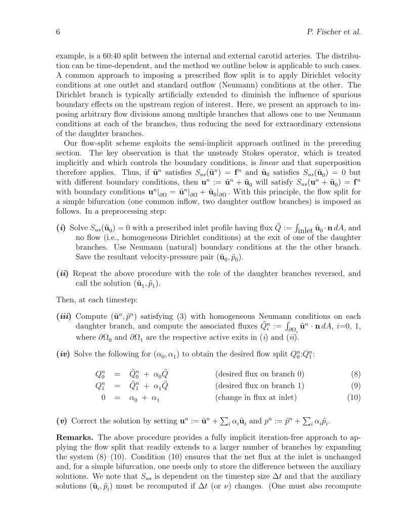
Figure 2. Velocity vectors near the outflow of an internal carotid artery: (left) uncorrected,(center) corrected, and (right) corrected minus uncorrected.

8 P. Fischer et al.

net gain in mean velocity over the extent of the layer. We typically choose the constantC such that the gain is equal to the mean velocity prior to the correction. One could,however, increase the gain if stronger fluctuations are encountered.

Results for the nozzle-based outflow condition are illustrated in Fig. 2. The left panelshows the velocity field for the standard (uncorrected Neumann) condition near the out-flow boundary of an internal carotid artery at Re ≈ 1400 (based on the peak flow rate andstenosis diameter). Inward-pointing velocity vectors can be seen at the exit boundary,and the simulation becomes catastrophically unstable within 100 timesteps beyond thispoint. The center panel shows the flow field computed with the outflow correction. Theflow is leaving the domain at all points along the outflow boundary and the simulation isstable for all time. The difference between the two cases (right) shows that the outflowtreatment does not pollute the solution upstream of the boundary.

4. Mesh Generation

Spectral element mesh generation shares much in common with its FE counterpart.Several important distinctions, however, place constraints on the SE meshes. First, theuse of matrix-free operator evaluation, which reduces the storage from O(EN6) to O(EN3)and work per evaluation from O(EN6) to O(EN4), is dependent upon the tensor-productforms (4). This reduction is most effectively achieved with hexahedral elements, whichmay be curved through the use of iso- or subparametric mappings from Ω to Ωe [6]. Second,the fact that typical orders are in the range N=8 to 16 implies roughly a thousandfoldreduction in the number of elements required compared to an FE mesh at comparableresolution. The reduction, while advantageous in reducing the size of the input files, placessignificant constraints on the mesh generation scheme. Consequently, we have developedan SE mesh generation scheme that is specific to vascular geometries [27,43].

Our mesh generation scheme employs a sweeping algorithm, in which disc-shaped slabsare meshed by using a standard O-grid configuration, as illustrated in Fig. 3. The slabsurfaces are identified with isosurfaces of conduction (potential) solutions satisfying ho-mogeneous Neumann conditions along the vessel wall. The isosurfaces are computed bynumerically solving a sequence of Laplace equations, one for each branch, in the compu-tational domain on a preliminary mesh comprising tetrahedral elements. Because of therobustness of the conduction problem, the preliminary mesh can be of almost arbitraryquality. The isosurfaces define a set of natural coordinate systems that have the desirableproperties of being orthogonal to the vessel walls and of being guaranteed to producenonintersecting cross-sections that could otherwise lead to vanishing Jacobians associ-ated with the transformation from Ω to Ωe. Through a judicious choice of conductionproblems, one can identify three principal isosurfaces that naturally trisect the bifurca-tion geometry, as depicted in Fig. 3b. This trisection leads to a decomposition of thebifurcation into three branches, each of which is individually meshed with the sweepingalgorithm. The advantages of the conduction-based approach is that it can be automated(starting with a segmented stack, mesh generation requires a matter of minutes on a work-station [43]) and it produces high-quality all-hexahedral meshes with a minimum numberof topology-induced defects.


Figure 3. Swept templates, projected onto isopotential surfaces, for hexahedral meshgeneration in a carotid bifurcation geometry. The closeup on the right shows the princi-pal isosurfaces from the three conduction problems that provide a uniquely determinedtrisection of the domain into independently swept branches [43].

5. Resolution Requirements

An important component of any numerical study is the establishment of adequateresolution. This is particularly challenging in turbulent flows because one can expect toconverge only in the mean and higher-order statistics, which require long-time simulationsto eliminate natural fluctuations as a source of variance. For pulsatile turbulent flows,it is necessary to use phase averaging, in which one samples the solution at a certainphase of the cardiac cycle over a large number of cycles and then averages these results.Experiments in the transitional flow regime have shown that relatively slow pulsatilitycoupled to rapidly evolving turbulence merely acts as a switch that turns the turbulenceon or off and does not materially change the turbulent state [24,1]. Thus, given thelength of the cardiac cycle (>10 flow-through times for a typical bifurcation model) andthe number of samples required to reach a statistically stationary state, it is preferableto test for grid convergence by simply using steady inlet conditions at the peak Reynoldsnumbers. One can then exploit temporal homogeneity and ergodicity to obtain mean andrms velocity distributions that can be used for convergence tests.

As with its global spectral counterpart, the standard convergence procedure for thespectral element method is to increase the polynomial degree N for a fixed number ofelements E. It is also possible, however, to use an adaptive procedure in which onerefines the mesh and varies the polynomial degree locally to obtain optimal convergencerates, as is done with hp finite element methods [21,36]. Our general approach has been toconstruct a mesh that is finest in the region of interest, starting with relatively low degree(typ., N=4), and to then increase N as we increase the Reynolds number. We typicallyconstruct the mesh such that, at the target Reynolds number, N=8-12 will be sufficient.This range of N is typically optimal for the performance of our spectral element code

10 P. Fischer et al.

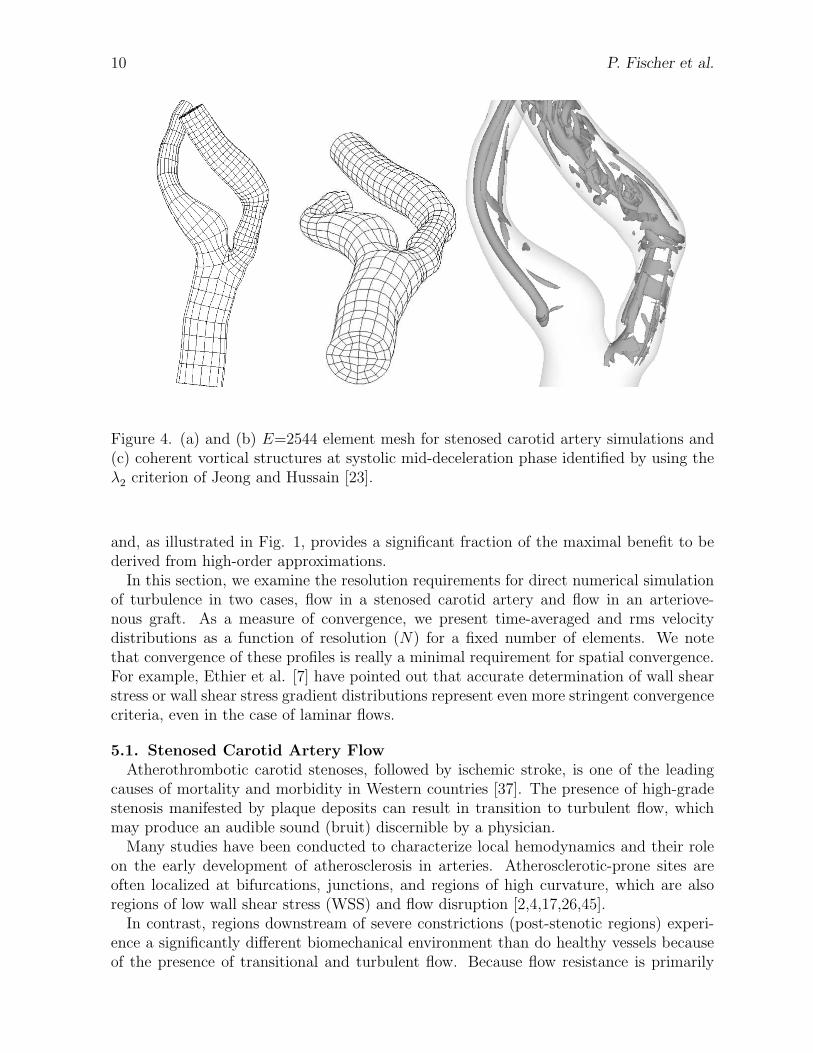
Figure 4. (a) and (b) E=2544 element mesh for stenosed carotid artery simulations and(c) coherent vortical structures at systolic mid-deceleration phase identified by using theλ2 criterion of Jeong and Hussain [23].

and, as illustrated in Fig. 1, provides a significant fraction of the maximal benefit to bederived from high-order approximations.

In this section, we examine the resolution requirements for direct numerical simulationof turbulence in two cases, flow in a stenosed carotid artery and flow in an arteriove-nous graft. As a measure of convergence, we present time-averaged and rms velocitydistributions as a function of resolution (N) for a fixed number of elements. We notethat convergence of these profiles is really a minimal requirement for spatial convergence.For example, Ethier et al. [7] have pointed out that accurate determination of wall shearstress or wall shear stress gradient distributions represent even more stringent convergencecriteria, even in the case of laminar flows.

5.1. Stenosed Carotid Artery FlowAtherothrombotic carotid stenoses, followed by ischemic stroke, is one of the leading

causes of mortality and morbidity in Western countries [37]. The presence of high-gradestenosis manifested by plaque deposits can result in transition to turbulent flow, whichmay produce an audible sound (bruit) discernible by a physician.

Many studies have been conducted to characterize local hemodynamics and their roleon the early development of atherosclerosis in arteries. Atherosclerotic-prone sites areoften localized at bifurcations, junctions, and regions of high curvature, which are alsoregions of low wall shear stress (WSS) and flow disruption [2,4,17,26,45].

In contrast, regions downstream of severe constrictions (post-stenotic regions) experi-ence a significantly different biomechanical environment than do healthy vessels becauseof the presence of transitional and turbulent flow. Because flow resistance is primarily


0 0.5 1 1.5 2 2.50

1

2

3

4

5

6

7

(a)

(b)

(c)

(d)

(e)

(f)

u (

m/s

)

time (s) 100

101

102

103

10−10

10−8

10−6

10−4

10−2

f (Hz)

Exx

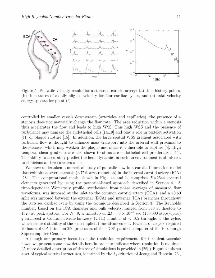
Figure 5. Pulsatile velocity results for a stenosed carotid artery: (a) time history points,(b) time traces of axially aligned velocity for four cardiac cycles, and (c) axial velocityenergy spectra for point (f).

controlled by smaller vessels downstream (arterioles and capillaries), the presence of astenosis does not materially change the flow rate. The area reduction within a stenosisthus accelerates the flow and leads to high WSS. This high WSS and the presence ofturbulence may damage the endothelial cells [14,19] and play a role in platelet activation[41] or plaque rupture [15]. In addition, the large spatial WSS gradient associated withturbulent flow is thought to enhance mass transport into the arterial wall proximal tothe stenosis, which may weaken the plaque and make it vulnerable to rupture [5]. Hightemporal shear gradients are also shown to stimulate endothelial cell proliferation [44].The ability to accurately predict the hemodynamics in such an environment is of interestto clinicians and researchers alike.

We have undertaken a numerical study of pulsatile flow in a carotid bifurcation modelthat exhibits a severe stenosis (∼75% area reduction) in the internal carotid artery (ICA)[28]. The computational mesh, shown in Fig. 4a and b, comprises E=2544 spectralelements generated by using the potential-based approach described in Section 4. Atime-dependent Womersely profile, synthesized from phase averages of measured flowwaveforms, was imposed at the inlet to the common carotid artery (CCA), and a 40:60split was imposed between the external (ECA) and internal (ICA) branches throughoutthe 0.75 sec cardiac cycle by using the technique described in Section 3. The Reynoldsnumber, based on the ICA diameter and bulk velocity, ranged from 380 at diastole to1320 at peak systole. For N=9, a timestep of ∆t = 5 × 10−6 sec (150,000 steps/cycle)guaranteed a Courant-Freidrichs-Lewy (CFL) number of < 0.5 throughout the cylce,which ensured stability of the semi-implicit time advancement. Each cardiac cycle required20 hours of CPU time on 256 processors of the TCS1 parallel computer at the PittsburghSupercomputer Center.

Although our primary focus is on the resolution requirements for turbulent vascularflows, we present some flow details here in order to indicate where resolution is required.(A more detailed description of this set of simulations is provided in [28].) Figure 4c showsa set of typical vortical structures, identified by the λ2 criterion of Jeong and Hussein [23],


(a)

2.4 m/s

(b) (c) (d)

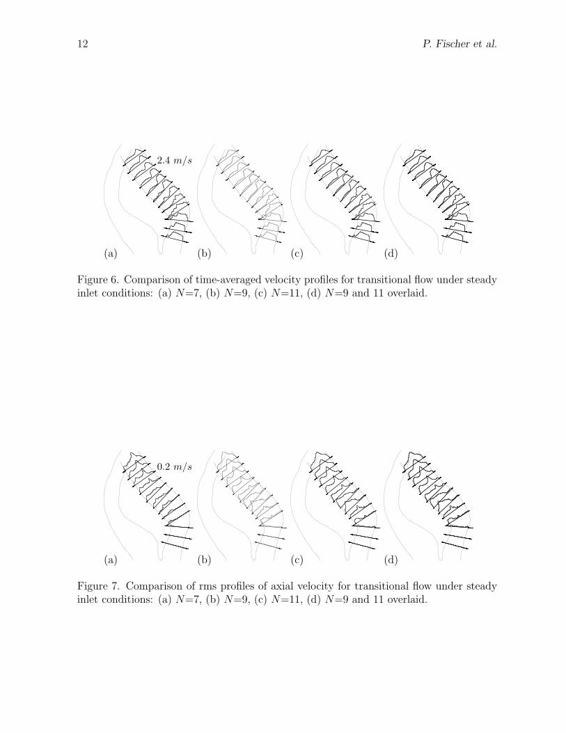
Figure 6. Comparison of time-averaged velocity profiles for transitional flow under steadyinlet conditions: (a) N=7, (b) N=9, (c) N=11, (d) N=9 and 11 overlaid.

(a)

0.2 m/s

(b) (c) (d)

Figure 7. Comparison of rms profiles of axial velocity for transitional flow under steadyinlet conditions: (a) N=7, (b) N=9, (c) N=11, (d) N=9 and 11 overlaid.


Graft

DVS

PVS

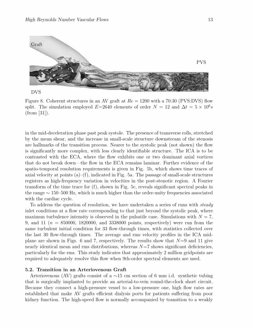
Figure 8. Coherent structures in an AV graft at Re = 1200 with a 70:30 (PVS:DVS) flowsplit. The simulation employed E=2640 elements of order N = 12 and ∆t = 5 × 106s(from [31]).

in the mid-deceleration phase past peak systole. The presence of transverse rolls, stretchedby the mean shear, and the increase in small-scale structure downstream of the stenosisare hallmarks of the transition process. Nearer to the systolic peak (not shown) the flowis significantly more complex, with less clearly identifiable structure. The ICA is to becontrasted with the ECA, where the flow exhibits one or two dominant axial vorticesthat do not break down—the flow in the ECA remains laminar. Further evidence of thespatio-temporal resolution requirements is given in Fig. 5b, which shows time traces ofaxial velocity at points (a)–(f), indicated in Fig. 5a. The passage of small-scale structuresregisters as high-frequency variation in velocities in the post-stenotic region. A Fouriertransform of the time trace for (f), shown in Fig. 5c, reveals significant spectral peaks inthe range ∼ 150–500 Hz, which is much higher than the order-unity frequencies associatedwith the cardiac cycle.

To address the question of resolution, we have undertaken a series of runs with steadyinlet conditions at a flow rate corresponding to that just beyond the systolic peak, wheremaximun turbulence intensity is observed in the pulsatile case. Simulations with N = 7,9, and 11 (n = 850000, 1820000, and 3338000 points, respectively) were run from thesame turbulent initial condition for 33 flow-through times, with statistics collected overthe last 30 flow-through times. The average and rms velocity profiles in the ICA mid-plane are shown in Figs. 6 and 7, respectively. The results show that N=9 and 11 givenearly identical mean and rms distributions, whereas N=7 shows significant deficiencies,particularly for the rms. This study indicates that approximately 2 million gridpoints arerequired to adequately resolve this flow when 9th-order spectral elements are used.

5.2. Transition in an Arteriovenous GraftArteriovenous (AV) grafts consist of a ∼15 cm section of 6 mm i.d. synthetic tubing

that is surgically implanted to provide an arterial-to-vein round-the-clock short circuit.Because they connect a high-pressure vessel to a low-pressure one, high flow rates areestablished that make AV grafts efficient dialysis ports for patients suffering from poorkidney function. The high-speed flow is normally accompanied by transition to a weakly


−3 −2 −1 0 1 2 3 4 5

−1.5

−1

−0.5

0

0.5

1

1.5

2U0

N = 12N = 10N = 7

(a)

x/d

−3 −2 −1 0 1 2 3 4 5

−1.5

−1

−0.5

0

0.5

1

1.5

U0 (b)

x/d

X

Y

Z

−3 −2 −1 0 1 2 3 4 5

−1.5

−1

−0.5

0

0.5

1

1.5

U0 (c)

x/d

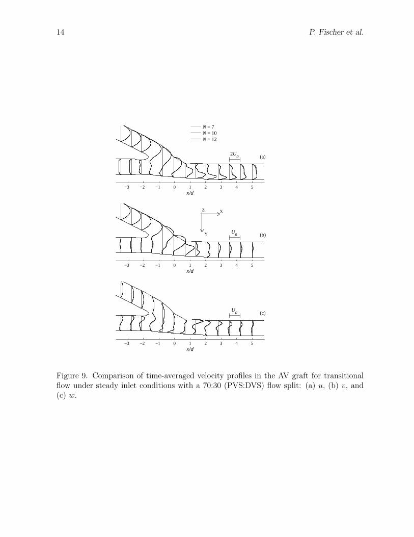
Figure 9. Comparison of time-averaged velocity profiles in the AV graft for transitionalflow under steady inlet conditions with a 70:30 (PVS:DVS) flow split: (a) u, (b) v, and(c) w.


0.5U0 (a)

N = 12N = 10N = 7

N = 12N = 10N = 7

N = 12N = 10N = 7

0.5U0 (b)

−3 −2 −1 0 1 2 3 4 5

−1.5

−1

−0.5

0 0.5U0 (c)

x/d

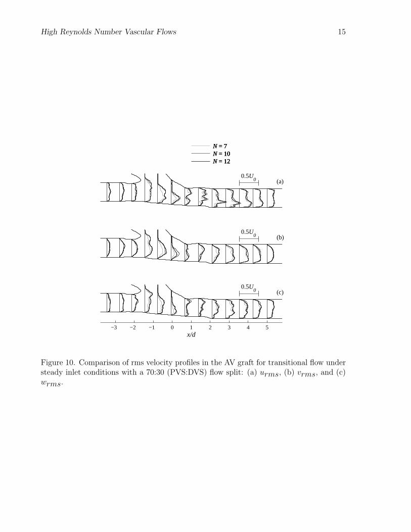
Figure 10. Comparison of rms velocity profiles in the AV graft for transitional flow understeady inlet conditions with a 70:30 (PVS:DVS) flow split: (a) urms, (b) vrms, and (c)wrms.


turbulent state, manifested as a 200–300 Hz vibration at the vein wall [29,32]. This high-frequency excitation is thought to lead to intimal hyperplasia, which can lead to completeocclusion of the vein and graft failure within six months of implant. We are investigatingthe mechanisms leading to transition in subject-specific AV-graft models with the aimof reducing turbulence through improved geometries. Detailed comparisons with laserDoppler anemometry (LDA) measurements are presented in [31]. Results for a pulsatileflow study are given in [29], and the influence of the flow division between the proximalvenous segment (PVS) and distal venous segment (DVS) is discussed in [30].

Figure 8 shows a typical turbulent case when there is a 70:30 split between the PVSand DVS. Significant small-scale structures are generated downstream (toward the heart)of the anastomosis in the PVS, which channels the majority of the flow. Steady graftinlet conditions are imposed, with a mean (cross-sectional average) velocity of U0. TheReynolds number based on the graft diameter is Re := U0D/ν = 1200. The SEM solutionwas computed with E=2640 elements of order 12 (4.5 million gridpoints).

A grid independence study was performed at Reynolds number 1200 with a flow splitof 70:30, corresponding to the conditions shown in Fig. 8. Comparisons of time-averagedvelocity and root-mean-square (rms) of the velocity fluctuation with N = 7, 10, and 12for the 70:30 flow division are shown in Figs. 9 and 10, respectively. Statistics weregathered for 1 second after an initial transient of 0.15 seconds, which was not included inthe statistics. (For comparison, the mean flow-through time is ∼0.1 seconds in vivo units;D=6 mm and U0 = 649 mm/sec). The time-averaged velocity did not show significantchange for N=7, 10 or 12. However, the rms of velocity showed noticeable change betweenpolynomial orders, even in the results of N = 12. This dependency could be attributedto statistical variance over the collection period or indicate the need for still higher gridresolution. However, the results with N = 12 are adequate for demonstrating the primaryfeatures of the flow since the rms of velocity is observed to be bounded in Fig. 10 withincreasing polynomial order.

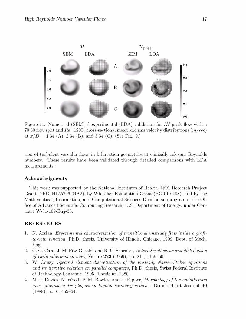
Based on these grid independence studies, the numerical results with N = 12 were usedfor validation with experimental measurements obtained using laser Doppler anemometry(LDA), as described in [31]. Figure 11 shows a comparison of mean and rms cross-sectionalvelocity distributions in the turbulent PVS flow with a 70:30 flow split at Re=1200.Measurements were taken at stations x/D=1.34, 2.34, and 3.34 (see Fig. 9). It is clearthat the N=12 case is able to accurately predict both the mean flow distribution and therms fluctuations.

6. Summary

We have presented methodology and convergence results for the application of a high-order spectral element method to the simulation of vascular flows. We have demonstrateda fast implicit approach to imposition of arbitrary flow division among daughter branchesthat avoids the need for extraordinary extensions or iteration to determine exit pressures.We have also developed an outflow treatment for turbulent flows that eliminates incomingcharacteristics that can destabilize the simulation. We have demonstrated some of thedesirable transport properties of high-order discretizations that are relevant to turbulentflows and shown that roughly 2–4 million points are required for direct numerical simula-


uSEM LDA

urms

SEM LDA

A

B

C

Figure 11. Numerical (SEM) / experimental (LDA) validation for AV graft flow with a70:30 flow split and Re=1200: cross-sectional mean and rms velocity distributions (m/sec)at x/D = 1.34 (A), 2.34 (B), and 3.34 (C). (See Fig. 9.)

tion of turbulent vascular flows in bifurcation geometries at clinically relevant Reynoldsnumbers. These results have been validated through detailed comparisons with LDAmeasurements.

Acknowledgments

This work was supported by the National Institutes of Health, RO1 Research ProjectGrant (2RO1HL55296-04A2), by Whitaker Foundation Grant (RG-01-0198), and by theMathematical, Information, and Computational Sciences Division subprogram of the Of-fice of Advanced Scientific Computing Research, U.S. Department of Energy, under Con-tract W-31-109-Eng-38.

REFERENCES

1. N. Arslan, Experimental characterization of transitional unsteady flow inside a graft-to-vein junction, Ph.D. thesis, University of Illinois, Chicago, 1999, Dept. of Mech.Eng.

2. C. G. Caro, J. M. Fitz-Gerald, and R. C. Schroter, Arterial wall shear and distributionof early atheroma in man, Nature 223 (1969), no. 211, 1159–60.

3. W. Couzy, Spectral element discretization of the unsteady Navier-Stokes equationsand its iterative solution on parallel computers, Ph.D. thesis, Swiss Federal Instituteof Technology-Lausanne, 1995, Thesis nr. 1380.

4. M. J. Davies, N. Woolf, P. M. Rowles, and J. Pepper, Morphology of the endotheliumover atherosclerotic plaques in human coronary arteries, British Heart Journal 60(1988), no. 6, 459–64.


5. N. DePaola, M.A. Gimbrone, P.F. Davies, and C.F. Dewey, Vascular endotheliumresponds to fluid shear stress gradients, Arteriosclerosis Thrombosis 12 (1992), no. 11,1254–7.

6. M.O. Deville, P.F. Fischer, and E.H. Mund, High-order methods for incompressiblefluid flow, Cambridge University Press, Cambridge, 2002.

7. C.R. Ethier, S. Prakash, D.A. Steinman, R.L. Leask, G.G. Couch, and M. Ojha,Steady flow separation patterns in a 45 degree junction, J. Fluid Mech. 411 (2000),1–38.

8. M. F. Fillinger, E. R. Reinitz, R. A. Schwartz, D. E. Resetarits, A. M. Paskanik, andC. E. Bredenberg, Beneficial effects of banding on venous intimal-medial hyperplasiain arteriovenous loop grafts, J. Vasc. Surg. 11 (1990), no. 4, 556–66.

9. P.F. Fischer, An overlapping Schwarz method for spectral element solution of the in-compressible Navier-Stokes equations, J. Comput. Phys. 133 (1997), 84–101.

10. P.F. Fischer, G.W. Kruse, and F. Loth, Spectral element methods for transitional flowsin complex geometries, J. Sci. Comput. 17 (2002), 81–98.

11. P.F. Fischer and J.W. Lottes, Hybrid Schwarz-multigrid methods for the spectral ele-ment method: Extensions to Navier-Stokes, Domain Decomposition Methods in Sci-ence and Engineering Series (R. Kornhuber, R. Hoppe, J. Priaux, O. Pironneau,O. Widlund, and J. Xu, eds.), Springer, Berlin, 2004.

12. P.F. Fischer, N.I. Miller, and H.M. Tufo, An overlapping Schwarz method for spec-tral element simulation of three-dimensional incompressible flows, Parallel Solution ofPartial Differential Equations (Berlin) (P. Bjørstad and M. Luskin, eds.), Springer,2000, pp. 158–180.

13. P.F. Fischer and J.S. Mullen, Filter-based stabilization of spectral element methods,Comptes rendus de l’Academie des sciences, Serie I- Analyse numerique 332 (2001),265–270.

14. D. L. Fry, Acute vascular endothelial changes associated with increased blood velocitygradients, Circulation Research 22 (1968), no. 2, 165–97.

15. S. D. Gertz and W. C. Roberts, Hemodynamic shear force in rupture of coronaryarterial atherosclerotic plaques, American Journal of Cardiology 66 (1990), no. 19,1368–72.

16. R. Gin, A.G. Straatman, and D.A. Steinman, A dual-pressure boundary condition foruse in simulations of bifurcating conduits, J. Biomech. Eng. 124 (2002), 617–619.

17. S. Glagov, C. K. Zarins, D.P. Giddens, and D.N. . Ku, Hemodynamics and atheroscle-rosis. insights and perspectives gained from studies of human arteries, Archives ofPathology and Laboratory Medicine 112 (1988), 1018–1031.

18. D. Gottlieb and S.A. Orszag, Numerical analysis of spectral methods: Theory andapplications, SIAM-CBMS, Philadelphia, 1977.

19. J. D. Hellums, The resistance to oxygen transport in the capillaries relative to that inthe surrounding tissue, Microvascular Research 13 (1977), no. 1, 131–6.

20. L.W. Ho, A Legendre spectral element method for simulation of incompressible un-steady viscous free-surface flows, Ph.D. thesis, Massachusetts Institute of Technology,1989, Cambridge, MA.

21. L.C. Hsu and C. Mavriplis, Adaptive meshes for the spectral element method, DomainDecomposition 9 Proc. (New York) (P. Bjørstad, M. Espedal, and D. Keyes, eds.), J.


Wiley, 1997, pp. 374–381.22. KJ Hutchison and E Karpinski, In vivo demonstration of flow recirculation and tur-

bulence downstrea stenoses in canine arteries, J. Biomech. 18 (1985), 285–296.23. J. Jeong and F. Hussain, On the identification of a vortex, J. Fluid Mech. 285 (1995),

69–94.24. P.S. Klebanoff, W.G. Cleveland, and K.D. Tidstrom, On the evolution of a turbulent

boundary layer induced by a three-dimensional roughness element, J. Fluid Mech. 92(1992), 101–187.

25. D. N. Ku, Blood flow in arteries, Annu. Rev. Fluid Mech. 29 (1997), 399–434.26. D. N. Ku, D. P. Giddens, C. K. Zarins, and S. Glagov, Pulsatile flow and atheroscle-

rosis in the human carotid bifurcation, Arteriosclerosis 5 (1985), no. 3, 293–302.27. S.E. Lee, Solution method for transitional flow in a vascular bifurcation based on

in vivo medical images, Master’s thesis, Univ. of Illinois, Chicago, 2002, Dept. ofMechanical Engineering.

28. S.E. Lee, S-W Lee, P.F. Fischer, H.S. Bassiouny, and F. Loth, Direct numerical simu-lation of transitional flow in a stenosed carotid bifurcation, J. Biomech. (submitted).

29. S.W. Lee, P.F. Fischer, F. Loth, T.J. Royston, J.K. Grogan, and H.S. Bassiouny, Flow-induced vein-wall vibration in an arteriovenous graft, J. of Fluids and Structures 20(2005), 837–852.

30. S.W. Lee, D.S. Smith, F. Loth, P.F. Fischer, and H.S. Bassiouny, Importance of flowdivision on transition to turbulence within an arteriovenous graft, J. Biomechanics inpress (2006).

31. , Numerical and experimental simulation of transitional flow in a blood vesseljunction, Num. Heat Transfer in press (2006).

32. F. Loth, N. Arslan, P. F. Fischer, C. D. Bertram, S. E. Lee, T. J. Royston, R. H.Song, W. E. Shaalan, and H. S. Bassiouny, Transitional flow at the venous anasto-mosis of an arteriovenous graft: Potential relationship with activation of the ERK1/2mechanotransduction pathway, ASME J. Biomech. Engr. 125 (2003), 49–61.

33. J. W. Lottes and P. F. Fischer, Hybrid multigrid/Schwarz algorithms for the spectralelement method, J. Sci. Comput. 24 (2005), 45–78.

34. Y. Maday and A.T. Patera, Spectral element methods for the Navier-Stokes equations,State-of-the-Art Surveys in Computational Mechanics (A.K. Noor and J.T. Oden,eds.), ASME, New York, 1989, pp. 71–143.

35. Y. Maday, A.T. Patera, and E.M. Rønquist, An operator-integration-factor splittingmethod for time-dependent problems: Application to incompressible fluid flow, J. Sci.Comput. 5 (1990), 263–292.

36. C. Mavriplis, Adaptive mesh strategies for the spectral element method, Comput. Meth-ods Appl. Mech. Engrg. 116 (1994), 77–86.

37. C. J. Murray and A. D. Lopez, Alternative projections of mortality and disabilityby cause 1990-2020: Global burden of disease study, Lancet 349 (1997), no. 9064,1498–504.

38. S.A. Orszag, Spectral methods for problems in complex geometry, J. Comput. Phys.37 (1980), 70–92.

39. J.B. Perot, An analysis of the fractional step method, J. Comp. Phys. 108 (1993),51–58.


40. S. J. Ram, A. Magnasco, S. A. Jones, A. Barz, L. Zsom, S. Swamy, and W. D. Paulson,In vivo validation of glucose pump test for measurement of hemodialysis access flow,Am J Kidney Dis 42 (2003), no. 4, 752–60.

41. J. M. Ramstack, L. Zuckerman, and L. F. Mockros, Shear-induced activation ofplatelets, Journal of Biomechanics 12 (1979), no. 2, 113–25.

42. S.J. Sherwin and H.M. Blackburn, Three-dimensional instabilities and transition ofsteady and pulsatile axisymmetric stenotic flows, J. Fluid Mech. 533 (2005), 297–327.

43. C.S. Verma, P.F. Fischer, S.E. Lee, and F. Loth, An all-hex meshing strategy forbifurcation geometries in vascular flow simulation, Proc. of the 14th Int. MeshingRoundtable, San Diego, 2005.

44. C. R. White, M. Haidekker, X. Bao, and J. A. Frangos, Temporal gradients inshear, but not spatial gradients, stimulate endothelial cell proliferation, Circulation103 (2001), no. 20, 2508–13.

45. C. K. Zarins, D. P. Giddens, B. K. Bharadvaj, V. S. Sottiurai, R. F. Mabon, andS. Glagov, Carotid bifurcation atherosclerosis. quantitative correlation of plaque lo-calization with flow velocity profiles and wall shear stress, Circulation Research 53(1983), no. 4, 502–14.


The submitted manuscript has been created bythe University of Chicago as Operator of Ar-gonne National Laboratory (”Argonne”) underContract No. W-31-109-ENG-38 with the U.S.Department of Energy. The U.S. Governmentretains for itself, and others acting on its behalf,a paid-up, nonexclusive, irrevocable worldwidelicense in said article to reproduce, preparederivative works, distribute copies to the pub-lic, and perform publicly and display publicly,by or on behalf of the Government.

Simulation of High Reynolds Number Vascular Flowsfischer/pubhtml/high_re.pdfSimulation of High Reynolds Number Vascular Flows Paul F. Fischer,a Francis Loth,b Seung E. Lee,c Sang-Wook

Documents