SIMULATION OF HELICOPTER AERODYNAMICS IN ... - CORE

SIMULATION OF HELICOPTER AERODYNAMICS IN THEVICINITY OF AN OBSTACLE USING A FREE WAKE PANEL

METHOD

Matthias Schmid, [email protected],DLR Institute of Aerodynamics and Flow Technology (Germany)

Abstract

In the present paper the influence of a helicopter wake on an idealized obstacle and vice versa is investigated.Simulations made by using an unsteady panel method are compared to experimental results from a wind tunneltest campaign. Various positions relative to the obstacle and two different wind conditions are investigated. A verygood accordance of the panel method to the experimental data can be shown for most of the test cases withoutwind. Only those positions where the helicopter rotor is in a recirculating flow field differ from the measuredvalues. For the test cases under head wind condition the accordance is not as good as without wind. Here theflow regions under influence of viscous effects are wider and the predictions made by the panel method havelarger offsets.

1 INTRODUCTION

Helicopters often have to operate in highly challeng-ing environments. Flights at low heights as well aslandings in confined areas are customary to currenthelicopter mission profiles. For example an emer-gency rescue helicopter has to land at very differentspots, at the roof of a hospital or near to a place ofan accident. The surroundings differ completely andalso do the aerodynamics. The rotor wakes formingin the vicinity of buildings or the ground can be verycomplex and influence the aerodynamics of the heli-copter. Therefore the workload of the pilot can be sig-nificantly increased or the performance and handlingqualities of the helicopter can be degraded.

Because of the huge number of possible flight sce-narios a fast and reliable simulation method is neededto investigate the various flight scenarios. The usabil-ity of a inviscid and incompressible free wake panelmethod will be explored in this paper.

All investigations are realized in context of the GAR-TEUR Action Group 22: “Forces on Obstacles in Ro-tor Wake” [1]. Subject of this collaboration is a sys-tematic investigation of the influence of the rotor wakeon an obstacle and vice versa. Four research cen-tres (CIRA (I), DLR (D), NLR (NL), ONERA (F)) andthree universities (NTUA (GR), Politecnico di Milano(I), University of Glasgow (UK)) contributed to this ac-tion group, either by providing measurement resultsor by carrying out numerical simulations of various fi-delity. Several scenarios of a helicopter flight in theproximity of an obstacle have been investigated.

2 SETUP

2.1 Experimental Setup

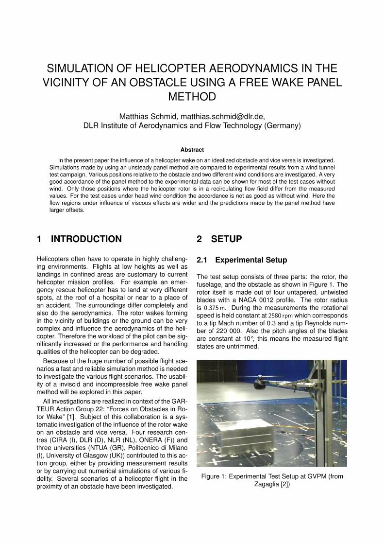
The test setup consists of three parts: the rotor, thefuselage, and the obstacle as shown in Figure 1. Therotor itself is made out of four untapered, untwistedblades with a NACA 0012 profile. The rotor radiusis 0.375m. During the measurements the rotationalspeed is held constant at 2580 rpm which correspondsto a tip Mach number of 0.3 and a tip Reynolds num-ber of 220 000. Also the pitch angles of the bladesare constant at 10°, this means the measured flightstates are untrimmed.

Figure 1: Experimental Test Setup at GVPM (fromZagaglia [2])

The fuselage design is inspired by a MD-500 fuse-lage and it contains a six-component balance to mea-sure the forces and moments acting on the rotor. Thesuspension of the model takes place over a stingmounted at the tail boom. The actual height is mea-sured directly at the helicopter model so any bendingof the suspension does not have to be considered.

Third part is the obstacle. It is a parallelepiped withsharp edges. The dimensions are 0.8m x 1.0m x0.45m. It is equipped with various pressure taps forsteady and unsteady pressure measurements.

All experiments are carried out in the wind tunnel“Galleria del Vento del Politecnico di Milano” (GVPM)both with and without head wind. The test setup isshown in Figure 1 from Zagaglia [2]. All experimentaldata is also taken from Zagaglia [2].

2.2 Test Cases

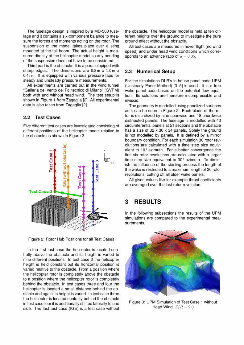
Five different test cases are investigated consisting ofdifferent positions of the helicopter model relative tothe obstacle as shown in Figure 2.

Figure 2: Rotor Hub Positions for all Test Cases

In the first test case the helicopter is located cen-trally above the obstacle and its height is varied tonine different positions. In test case 2 the helicopterheight is held constant but its horizontal position isvaried relative to the obstacle. From a position wherethe helicopter rotor is completely above the obstacleto a position where the helicopter rotor is completelybehind the obstacle. In test cases three and four thehelicopter is located a small distance behind the ob-stacle and again its height is varied. In test case threethe helicopter is located centrally behind the obstaclein test case four it is additionally shifted laterally to oneside. The last test case (IGE) is a test case without

the obstacle. The helicopter model is held at ten dif-ferent heights over the ground to investigate the pureground effect without the obstacle.

All test cases are measured in hover flight (no windspeed) and under head wind conditions which corre-sponds to an advance ratio of µ = 0.05.

2.3 Numerical Setup

For the simulations DLR’s in-house panel code UPM(Unsteady Panel Method) [3–5] is used. It is a freewake panel code based on the potential flow equa-tion. Its solutions are therefore incompressible andinviscid.

The geometry is modelled using panelized surfacesas it can be seen in Figure 2. Each blade of the ro-tor is discretized by nine spanwise and 18 chordwisedistributed panels. The fuselage is modelled with 43circumferential panels at 51 sections and the obstaclehas a size of 32 x 30 x 34 panels. Solely the groundis not modelled by panels. It is defined by a mirrorboundary condition. For each simulation 30 rotor rev-olutions are calculated with a time step size equiv-alent to 10° azimuth. For a better convergence thefirst six rotor revolutions are calculated with a largertime step size equivalent to 30° azimuth. To dimin-ish the influence of the starting process the length ofthe wake is restricted to a maximum length of 20 rotorrevolutions, cutting off all older wake panels.

All given values like for example thrust coefficientsare averaged over the last rotor revolution.

3 RESULTS

In the following subsections the results of the UPMsimulations are compared to the experimental mea-surements.

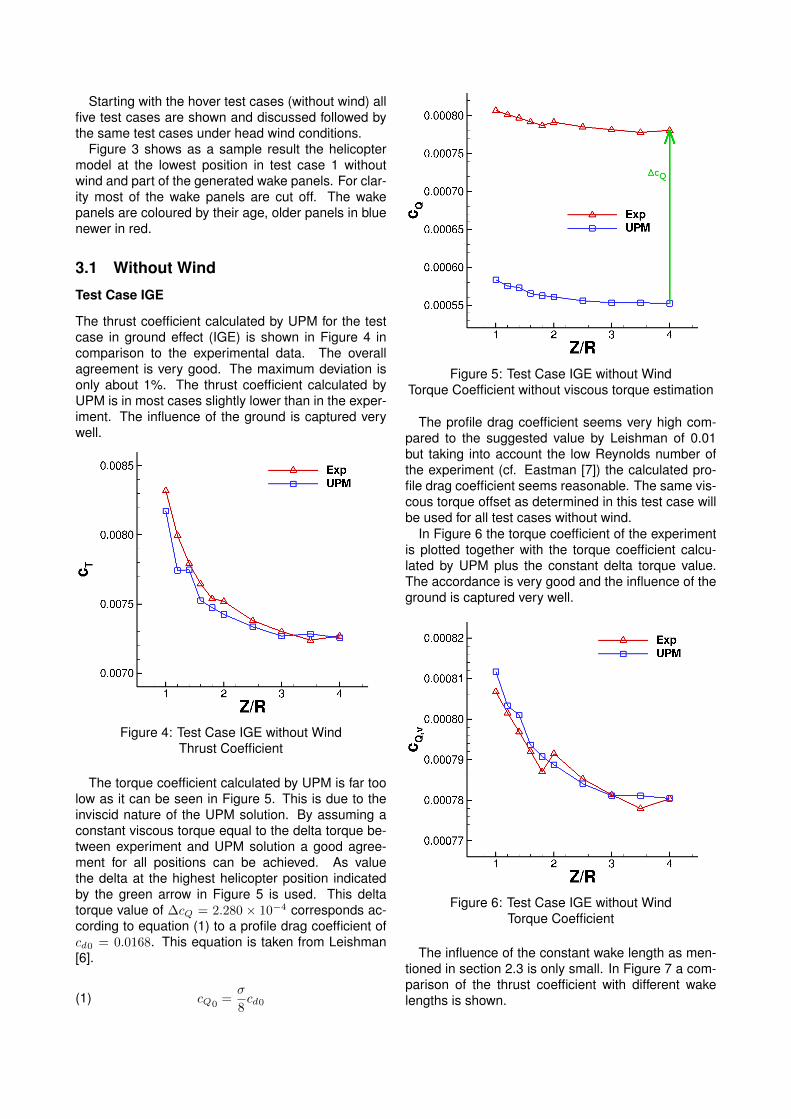
Figure 3: UPM Simulation of Test Case 1 withoutHead Wind, Z/R = 2.0

Starting with the hover test cases (without wind) allfive test cases are shown and discussed followed bythe same test cases under head wind conditions.

Figure 3 shows as a sample result the helicoptermodel at the lowest position in test case 1 withoutwind and part of the generated wake panels. For clar-ity most of the wake panels are cut off. The wakepanels are coloured by their age, older panels in bluenewer in red.

3.1 Without Wind

Test Case IGE

The thrust coefficient calculated by UPM for the testcase in ground effect (IGE) is shown in Figure 4 incomparison to the experimental data. The overallagreement is very good. The maximum deviation isonly about 1%. The thrust coefficient calculated byUPM is in most cases slightly lower than in the exper-iment. The influence of the ground is captured verywell.

Figure 4: Test Case IGE without WindThrust Coefficient

The torque coefficient calculated by UPM is far toolow as it can be seen in Figure 5. This is due to theinviscid nature of the UPM solution. By assuming aconstant viscous torque equal to the delta torque be-tween experiment and UPM solution a good agree-ment for all positions can be achieved. As valuethe delta at the highest helicopter position indicatedby the green arrow in Figure 5 is used. This deltatorque value of ∆cQ = 2.280 × 10−4 corresponds ac-cording to equation (1) to a profile drag coefficient ofcd0 = 0.0168. This equation is taken from Leishman[6].

(1) cQ0 =σ

8cd0

Figure 5: Test Case IGE without WindTorque Coefficient without viscous torque estimation

The profile drag coefficient seems very high com-pared to the suggested value by Leishman of 0.01but taking into account the low Reynolds number ofthe experiment (cf. Eastman [7]) the calculated pro-file drag coefficient seems reasonable. The same vis-cous torque offset as determined in this test case willbe used for all test cases without wind.

In Figure 6 the torque coefficient of the experimentis plotted together with the torque coefficient calcu-lated by UPM plus the constant delta torque value.The accordance is very good and the influence of theground is captured very well.

Figure 6: Test Case IGE without WindTorque Coefficient

The influence of the constant wake length as men-tioned in section 2.3 is only small. In Figure 7 a com-parison of the thrust coefficient with different wakelengths is shown.

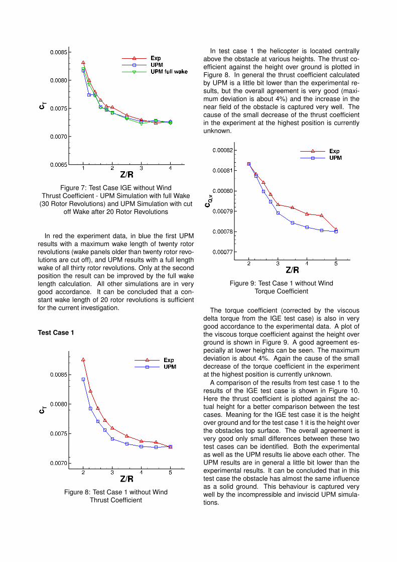
Figure 7: Test Case IGE without WindThrust Coefficient - UPM Simulation with full Wake

(30 Rotor Revolutions) and UPM Simulation with cutoff Wake after 20 Rotor Revolutions

In red the experiment data, in blue the first UPMresults with a maximum wake length of twenty rotorrevolutions (wake panels older than twenty rotor revo-lutions are cut off), and UPM results with a full lengthwake of all thirty rotor revolutions. Only at the secondposition the result can be improved by the full wakelength calculation. All other simulations are in verygood accordance. It can be concluded that a con-stant wake length of 20 rotor revolutions is sufficientfor the current investigation.

Test Case 1

Figure 8: Test Case 1 without WindThrust Coefficient

In test case 1 the helicopter is located centrallyabove the obstacle at various heights. The thrust co-efficient against the height over ground is plotted inFigure 8. In general the thrust coefficient calculatedby UPM is a little bit lower than the experimental re-sults, but the overall agreement is very good (maxi-mum deviation is about 4%) and the increase in thenear field of the obstacle is captured very well. Thecause of the small decrease of the thrust coefficientin the experiment at the highest position is currentlyunknown.

Figure 9: Test Case 1 without WindTorque Coefficient

The torque coefficient (corrected by the viscousdelta torque from the IGE test case) is also in verygood accordance to the experimental data. A plot ofthe viscous torque coefficient against the height overground is shown in Figure 9. A good agreement es-pecially at lower heights can be seen. The maximumdeviation is about 4%. Again the cause of the smalldecrease of the torque coefficient in the experimentat the highest position is currently unknown.

A comparison of the results from test case 1 to theresults of the IGE test case is shown in Figure 10.Here the thrust coefficient is plotted against the ac-tual height for a better comparison between the testcases. Meaning for the IGE test case it is the heightover ground and for the test case 1 it is the height overthe obstacles top surface. The overall agreement isvery good only small differences between these twotest cases can be identified. Both the experimentalas well as the UPM results lie above each other. TheUPM results are in general a little bit lower than theexperimental results. It can be concluded that in thistest case the obstacle has almost the same influenceas a solid ground. This behaviour is captured verywell by the incompressible and inviscid UPM simula-tions.

Figure 10: Test Case 1 and IGE without WindComparison of Thrust Coefficient

Test Case 2

In test case 2 the helicopter model is held at a con-stant height over ground of Z/R = 2.0 but its horizon-tal position is varied relative to the obstacle. In theFigures 11 and 12 the coefficients are plotted againstthe relative X-position. At a value of -1 the rotor iscompletely above the obstacle and at a value of +1the rotor is completely behind the obstacle.


The thrust coefficient as shown in Figure 11 is againin most cases a little bit too low, except at the secondlast position, where there is a kink in the experimentaldata, but the overall agreement is good. The thrustincrease over the obstacle is not as strong as in theexperiment and the maximum deviation of about 5%is identified at the position X/R = −1.


The torque coefficient is shown in Figure 12. Theagreement is especially good at the positions fromX/R = −1 to X/R = 0. The maximum deviation ofall positions is below 1%. Corresponding to test case1 it can be mentioned that there is more deviation inthe torque coefficient at larger heights. Although thehelicopter model is held at a constant height over theground in this test case its actual height is varyingwhether its position is over the obstacle or behind ofit.

Flow Field

For test case 2 additional Particle Image Velocimetry(PIV) pictures are available for a small part of the flowfield behind the obstacle. The PIV images for a rotorhub position at X/R = −1, X/R = 0, and X/R = 1will be compared to the corresponding UPM results.The positions of the PIV window (red rectangle) andthe helicopter model are indicated by the pictogram atthe center of the Figures 13-15. On the left side theexperimental measurements are shown on the rightside the results of UPM. The velocities in all shownflow fields are time averaged.

In Figure 13 the helicopter model is hovering abovethe obstacle. In the experiment a flow stream ofhigher velocities separated from the obstacle top sur-face can be identified, forming a clockwise rotatingvortex at the obstacle side. In the UPM solution thisflow stream and also the vortex is not visible. Herethe higher velocities are bound to the left and loweredge of the window.

In the next Figure (Figure 14) the helicopter modelis hovering above the edge of the obstacle. In theexperiment the region of higher velocities is clearlybigger as in the previous case and it can be seen that

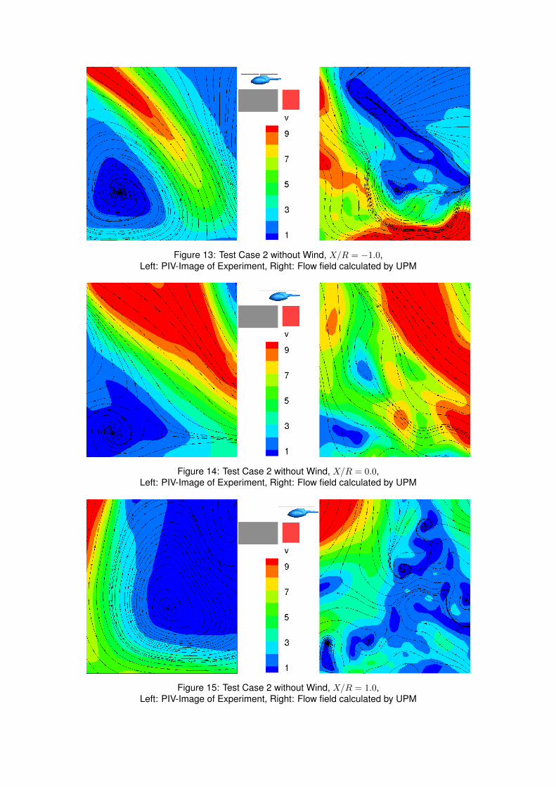
Figure 13: Test Case 2 without Wind, X/R = −1.0,Left: PIV-Image of Experiment, Right: Flow field calculated by UPM

Figure 14: Test Case 2 without Wind, X/R = 0.0,Left: PIV-Image of Experiment, Right: Flow field calculated by UPM

Figure 15: Test Case 2 without Wind, X/R = 1.0,Left: PIV-Image of Experiment, Right: Flow field calculated by UPM

the flow is coming from two directions. First from thetop left, separated from the obstacle top surface, asbefore. Second directly from above from the rear partof the rotor disc. A small vortex on the obstacle sideis forming also in this case but now rotating counter-clockwise. In the UPM solution only the second partof the stream is visible. The flow separated from theobstacle is as before not present in the UPM solution.Also in this case there is no vortex forming at the ob-stacle side in the UPM solution.

In the last Figure (Figure 15) the helicopter modelis hovering behind the obstacle. In the experimentaldata on the left hand side the rotor downwash canbe seen. The flow is distracted at the obstacle sidewall and the ground so that a huge counter-clockwiserotating vortex is forming. In the UPM solution thehigher velocities at the left side are also visible butthe vortex is not present.

These big differences between the experimentalflow field and the results of UPM can be explainedby the inviscid nature of the UPM solution. The flowfields presented in the experiment are mainly influ-enced by the separation of the flow at the sharp edgesof the obstacle and a highly recirculating flow is estab-lished. Due to the inviscid nature of UPM this sepa-ration is not part of the UPM solution. Here the flowon the top surface of the obstacle is deflected at theedges and adheres to the obstacle side walls. Thisbehaviour of the UPM solution could be improved byinserting wake panels at the obstacle edges, but thisfeature is not implemented yet.

Test Case 3

In test case 3 the helicopter model is operated in thehighly recirculating flow field behind the obstacle. Thehelicopter model is positioned centrally behind the ob-stacle and its height is varied. The lowest position isat a relative height of Z/R = 1. With a relative obsta-cle height of Z/R = 1.2 the helicopter rotor is operat-ing below the top surface of the obstacle.

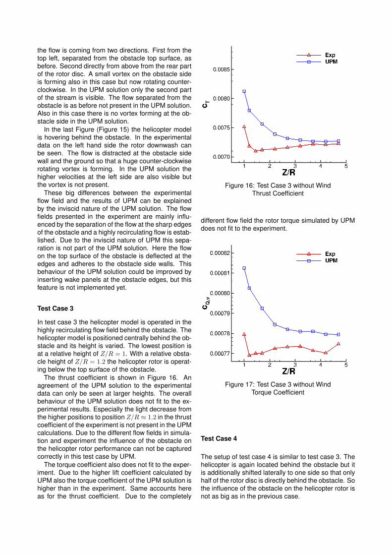
The thrust coefficient is shown in Figure 16. Anagreement of the UPM solution to the experimentaldata can only be seen at larger heights. The overallbehaviour of the UPM solution does not fit to the ex-perimental results. Especially the light decrease fromthe higher positions to position Z/R ≈ 1.2 in the thrustcoefficient of the experiment is not present in the UPMcalculations. Due to the different flow fields in simula-tion and experiment the influence of the obstacle onthe helicopter rotor performance can not be capturedcorrectly in this test case by UPM.

The torque coefficient also does not fit to the exper-iment. Due to the higher lift coefficient calculated byUPM also the torque coefficient of the UPM solution ishigher than in the experiment. Same accounts hereas for the thrust coefficient. Due to the completely


different flow field the rotor torque simulated by UPMdoes not fit to the experiment.


Test Case 4

The setup of test case 4 is similar to test case 3. Thehelicopter is again located behind the obstacle but itis additionally shifted laterally to one side so that onlyhalf of the rotor disc is directly behind the obstacle. Sothe influence of the obstacle on the helicopter rotor isnot as big as in the previous case.



The thrust coefficient is plotted in Figure 18. Theoverall agreement to the experimental data is in thiscase again very good. The influence of the obstacle isbecause of the further distance not as high as in theprevious test case. The thrust increase in the UPMsolutions is slightly higher than in the experiment.

The experimental data for the torque coefficient inthis test case as it can be seen in Figure 19 doesnot seem to be very reasonable. The torque increaseat larger heights and the offset of the torque valuesat Z/R ≈ 2.2 and Z/R ≈ 2.8 cannot be explainedby now as the thrust coefficient does not show anyanomalies. The agreement at lower heights is rela-tively good.

3.2 With Wind

In this chapter the same setup of the test cases asin the previous chapter are discussed but this timethe investigations are under head wind conditions withan inflow velocity of ≈ 5.0m/s resulting in a rotor ad-vance ratio of µ = 0.05. A sample result of the UPMsimulations under head wind condition is shown inFigure 20. Again for clarity only part of the wake pan-els are shown.

Figure 20: UPM Simulation of Test Case 2 underHead Wind Conditions, X/R = 0.0, Z/R = 2.0

The simulations under head wind conditions aremore demanding compared to the cases withoutwind. The wake panels generated at the rotor bladescannot spread uniformly in all directions and areblown back to the rotor disc where they interact withthe rotor blades and the newer wake panels. Forsome of the following simulations especially at lowerheights a periodic state could not be achieved. Thesesimulations are marked in the corresponding plots.

Any elastic bending of the rotor blades due to timevarying loads during the experiment cannot be mod-elled in the simulations due to the lack of appropri-ate measurements. So larger deviations are expectedthan without wind.

Test Case IGE

The thrust coefficients calculated by UPM for the testcase in ground effect compared to the experimentalresults are shown in Figure 21. It can be stated thatthe calculated thrust coefficients are in general higherthan the measured ones, but nonetheless the accor-dance is quite good, the maximum deviation is onlyabout 3%.

Same as in the cases without wind the torque coef-ficients calculated by UPM will be off-setted by a con-stant delta torque. This delta torque is obtained fromthe values of the UPM solution and the experiment inthe IGE test case with the helicopter hub at a heightof Z/R = 4. The delta torque in this test case under

Figure 21: Test Case IGE with WindThrust Coefficient

head wind condition is equal to ∆cQ = 2.416 × 10−4.This value corresponds to a profile drag coefficient ofcd0 = 0.0176 which is calculated with equation (2).This approximative equation is taken from Johnson[8].

(2) cQ0 =σ

8cd0

(1 + 4.6µ2

)The delta torque and also the profile drag coeffi-

cient in the IGE test case with wind is slightly higherthan in the case without wind. This is due to the largerviscous effects in forward flight and the neglect of anyelastic blade bending in the UPM simulations.

Figure 22: Test Case IGE with and without WindComparison of Thrust Coefficient

In Figure 22 a comparison of the thrust coefficientsof the IGE test cases with and without wind is shown.

The UPM results are shown in blue the experimentaldata in red. Results of the tests under head wind con-ditions are plotted with solid lines tests without windin dashed lines.

In general the influence of the ground on the thrustcoefficient under head wind conditions is not as highas in the same test case without wind as it can beseen in Figure 22. The thrust increase under headwind conditions is only about half the amount thanwithout wind. This behaviour is simulated very wellby UPM.

At larger heights under head wind conditions thethrust coefficient is increased and maintains at an al-most constant value until Z/R ≈ 2.5. Below thatheight a strong increase of the thrust coefficient canbe seen for both UPM and experiment, but for the ex-periment the thrust increase without wind is strongerso that at the lowest two positions the thrust withwind is lower than without. In the UPM results thethrust without wind is always lower than in the casewith wind. It can be concluded that the deviations forthe simulations under head wind conditions are largerthan without wind. This is due to the more compli-cated flow field and the more inexact rotor modellingdue to the neglect of any elastic bending of the rotorblades.

Figure 23: Test Case IGE with WindTorque Coefficient

The torque coefficient in the IGE test case is notcaptured as good as in the case without wind. Asshown in Figure 23 especially the strong increase atlower heights is not present in the UPM solution. Inthe experiment probably flow separation occurs at therotor blades due to the low Reynolds number and theadditional head wind. This causes the strong increasein the torque coefficient at lower heights. In groundeffect the induced velocity is reduced and thereforethe effective angle of attack is increased resulting in a

stronger separation near the ground. UPM does nottake viscous effects like flow separation into consid-eration. The assumption of a constant viscous torqueis especially for lower heights not correct in this testcase.

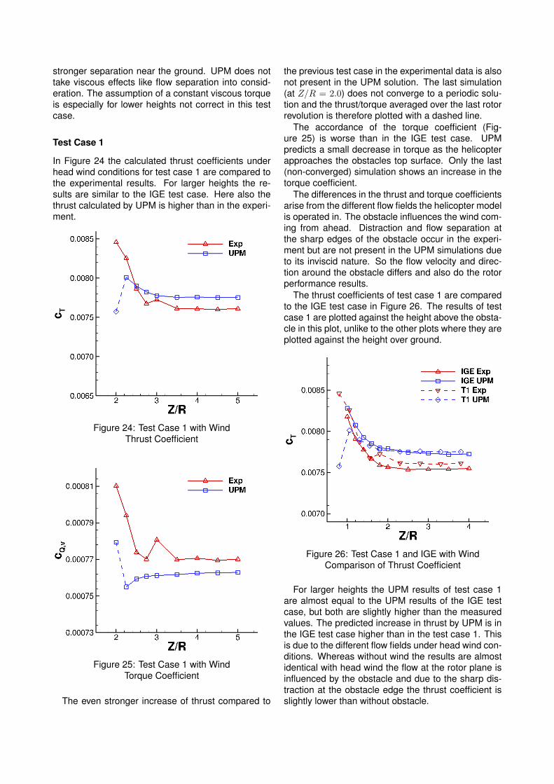
Test Case 1

In Figure 24 the calculated thrust coefficients underhead wind conditions for test case 1 are compared tothe experimental results. For larger heights the re-sults are similar to the IGE test case. Here also thethrust calculated by UPM is higher than in the experi-ment.

Figure 24: Test Case 1 with WindThrust Coefficient

Figure 25: Test Case 1 with WindTorque Coefficient

The even stronger increase of thrust compared to

the previous test case in the experimental data is alsonot present in the UPM solution. The last simulation(at Z/R = 2.0) does not converge to a periodic solu-tion and the thrust/torque averaged over the last rotorrevolution is therefore plotted with a dashed line.

The accordance of the torque coefficient (Fig-ure 25) is worse than in the IGE test case. UPMpredicts a small decrease in torque as the helicopterapproaches the obstacles top surface. Only the last(non-converged) simulation shows an increase in thetorque coefficient.

The differences in the thrust and torque coefficientsarise from the different flow fields the helicopter modelis operated in. The obstacle influences the wind com-ing from ahead. Distraction and flow separation atthe sharp edges of the obstacle occur in the experi-ment but are not present in the UPM simulations dueto its inviscid nature. So the flow velocity and direc-tion around the obstacle differs and also do the rotorperformance results.

The thrust coefficients of test case 1 are comparedto the IGE test case in Figure 26. The results of testcase 1 are plotted against the height above the obsta-cle in this plot, unlike to the other plots where they areplotted against the height over ground.

Figure 26: Test Case 1 and IGE with WindComparison of Thrust Coefficient

For larger heights the UPM results of test case 1are almost equal to the UPM results of the IGE testcase, but both are slightly higher than the measuredvalues. The predicted increase in thrust by UPM is inthe IGE test case higher than in the test case 1. Thisis due to the different flow fields under head wind con-ditions. Whereas without wind the results are almostidentical with head wind the flow at the rotor plane isinfluenced by the obstacle and due to the sharp dis-traction at the obstacle edge the thrust coefficient isslightly lower than without obstacle.

The experimental values show a small offset forthe higher helicopter positions. Here the thrust mea-sured over the obstacle is slightly higher than over theground. For lower helicopter positions the measuredvalues lie almost exactly above each other and forthe lowest two positions test case 1 again has somehigher thrust values compared to the IGE test case.

The offset in the experiment at larger heights is dueto the distracted and separated air flow from the ob-stacle. Under head wind conditions the obstacle dis-tracts the flow coming from ahead and the helicopterrotor gets an extra velocity component from below aslong as the rotor is not completely in the wake of theobstacle.

It can be concluded that the head wind conditionproduces a complex flow field around the obstaclewhich can not be simulated by UPM. Therefore theresults for the test cases under head wind conditionswill differ more than the test cases without wind.

Test Case 2

The thrust coefficients of test case 2 are shown in Fig-ure 27. In this test case the helicopter rotor is at aconstant height over the ground but its horizontal po-sition is varied in a way that the rotor is above, partlyabove, or behind the obstacle.


For the rotor hub positions of X/R = 1.0 untilX/R = 0.0 the UPM solution is in good accordance tothe experimental data. At these positions the wake ofthe rotor mainly flows to the ground which is at a dis-tance of Z/R = 2.0 which can be seen in Figure 29.In the last two simulations the wake of the rotor mainlyhits the obstacles top surface. The obstacle height isZ/R = 1.2 which means the helicopter rotor is at adistance of Z/R = 0.8 above the obstacle. At these

positions the UPM simulations do not converge to aperiodic state and the deviation of the results is veryhuge.


For the torque coefficient (shown in Figure 28) UPMpredicts a slight decrease for the three convergedsimulations as the helicopter approaches the obsta-cle. As in the previous test cases the predicted torquecoefficients are lower than in the experiment.

It can be seen that the influence of the obstacle inthe UPM simulations is only small for positions whereX/R > 0.0. For these simulations the generated wakepanels do not interact with the obstacle as it can beseen in Figure 29. Due to the constant head wind thewake panels are driven away from the obstacle andinteract only with the ground. When the helicopter ismoving forward the wake panels start to flow againstthe freestream velocity on the obstacles top surfaceand wrap around the obstacle. In a viscous flow thesewrapped structures would dissipate as time goes bybut in the inviscid UPM simulations they are main-tained and cause instabilities in the UPM solution.

Test Case 3

In test case 3 the helicopter model is located centrallybehind the obstacle and its height is been varied. Atits lowest position Z/R = 1.0 the helicopter rotor isbelow the obstacle top surface.

In Figure 30 the calculated thrust coefficient of UPMis plotted in comparison to the measured values fromthe experiment. Again there is a general offset andthe highest deviation is about 6%. The general trendfor the higher Z/R positions seems to be capturedcorrectly. Both the UPM results as well as the exper-imental data show a slow decrease of the thrust co-efficient when reducing the height. But in the experi-

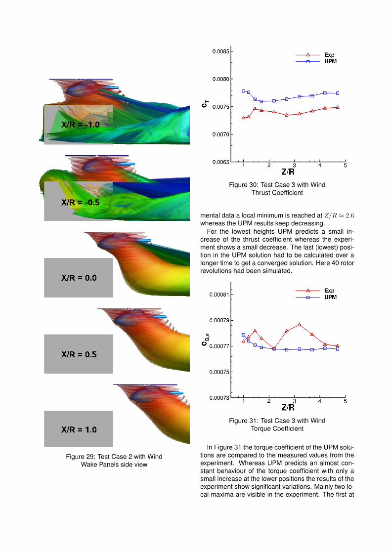
Figure 29: Test Case 2 with WindWake Panels side view


mental data a local minimum is reached at Z/R ≈ 2.6whereas the UPM results keep decreasing.

For the lowest heights UPM predicts a small in-crease of the thrust coefficient whereas the experi-ment shows a small decrease. The last (lowest) posi-tion in the UPM solution had to be calculated over alonger time to get a converged solution. Here 40 rotorrevolutions had been simulated.


In Figure 31 the torque coefficient of the UPM solu-tions are compared to the measured values from theexperiment. Whereas UPM predicts an almost con-stant behaviour of the torque coefficient with only asmall increase at the lower positions the results of theexperiment show significant variations. Mainly two lo-cal maxima are visible in the experiment. The first at

Z/R ≈ 3.0 is probably due to a shear layer emanatingfrom the obstacle. The second at Z/R ≈ 1.4 coin-cides with the position of a local maximum thrust inthe previous plot.

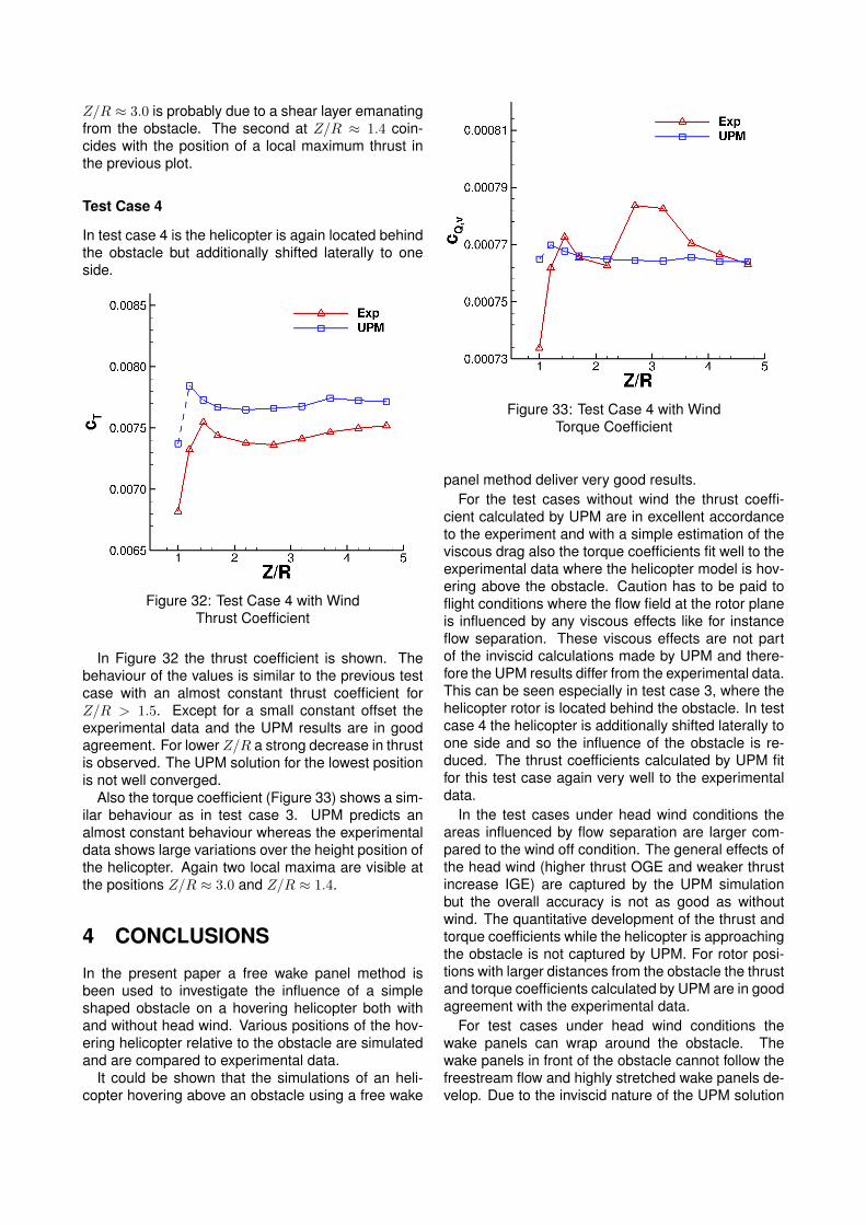
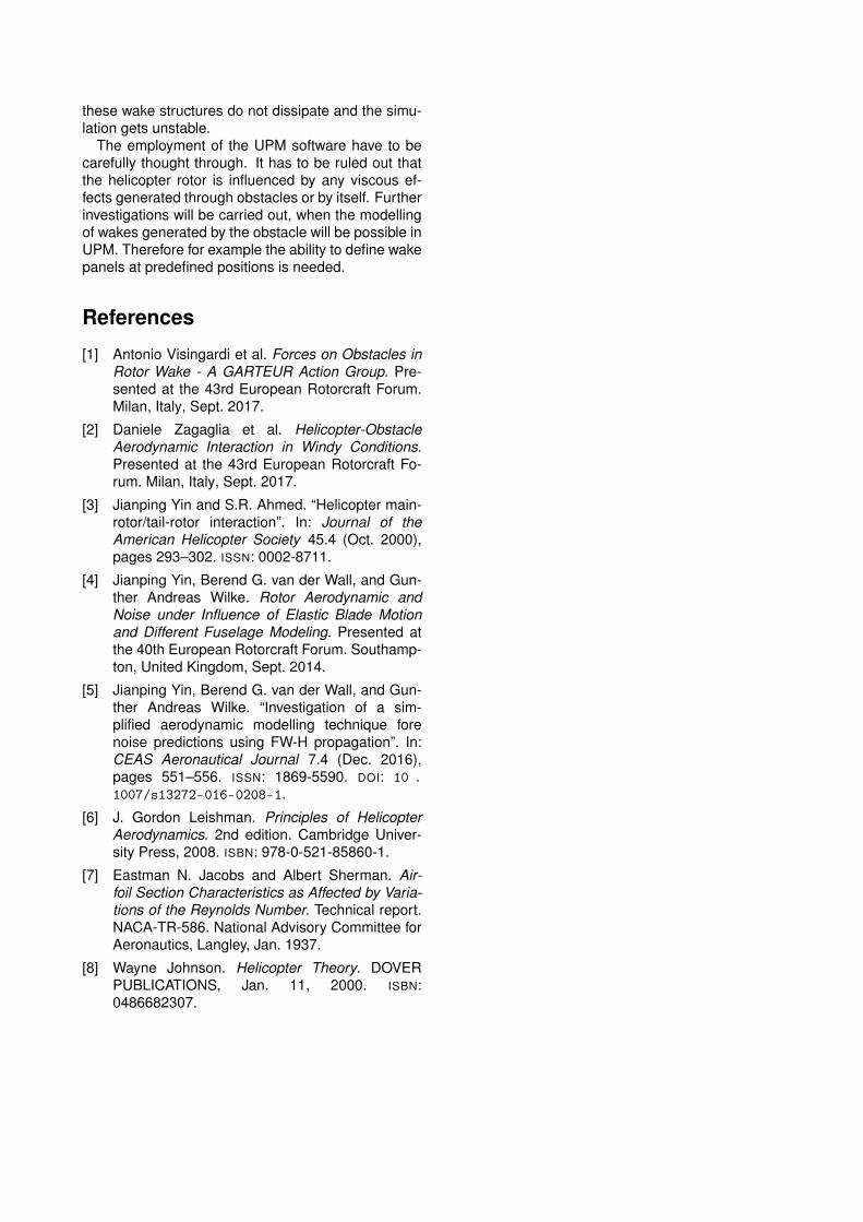
Test Case 4

In test case 4 is the helicopter is again located behindthe obstacle but additionally shifted laterally to oneside.


In Figure 32 the thrust coefficient is shown. Thebehaviour of the values is similar to the previous testcase with an almost constant thrust coefficient forZ/R > 1.5. Except for a small constant offset theexperimental data and the UPM results are in goodagreement. For lower Z/R a strong decrease in thrustis observed. The UPM solution for the lowest positionis not well converged.

Also the torque coefficient (Figure 33) shows a sim-ilar behaviour as in test case 3. UPM predicts analmost constant behaviour whereas the experimentaldata shows large variations over the height position ofthe helicopter. Again two local maxima are visible atthe positions Z/R ≈ 3.0 and Z/R ≈ 1.4.

4 CONCLUSIONS

In the present paper a free wake panel method isbeen used to investigate the influence of a simpleshaped obstacle on a hovering helicopter both withand without head wind. Various positions of the hov-ering helicopter relative to the obstacle are simulatedand are compared to experimental data.

It could be shown that the simulations of an heli-copter hovering above an obstacle using a free wake


panel method deliver very good results.For the test cases without wind the thrust coeffi-

cient calculated by UPM are in excellent accordanceto the experiment and with a simple estimation of theviscous drag also the torque coefficients fit well to theexperimental data where the helicopter model is hov-ering above the obstacle. Caution has to be paid toflight conditions where the flow field at the rotor planeis influenced by any viscous effects like for instanceflow separation. These viscous effects are not partof the inviscid calculations made by UPM and there-fore the UPM results differ from the experimental data.This can be seen especially in test case 3, where thehelicopter rotor is located behind the obstacle. In testcase 4 the helicopter is additionally shifted laterally toone side and so the influence of the obstacle is re-duced. The thrust coefficients calculated by UPM fitfor this test case again very well to the experimentaldata.

In the test cases under head wind conditions theareas influenced by flow separation are larger com-pared to the wind off condition. The general effects ofthe head wind (higher thrust OGE and weaker thrustincrease IGE) are captured by the UPM simulationbut the overall accuracy is not as good as withoutwind. The quantitative development of the thrust andtorque coefficients while the helicopter is approachingthe obstacle is not captured by UPM. For rotor posi-tions with larger distances from the obstacle the thrustand torque coefficients calculated by UPM are in goodagreement with the experimental data.

For test cases under head wind conditions thewake panels can wrap around the obstacle. Thewake panels in front of the obstacle cannot follow thefreestream flow and highly stretched wake panels de-velop. Due to the inviscid nature of the UPM solution

these wake structures do not dissipate and the simu-lation gets unstable.

The employment of the UPM software have to becarefully thought through. It has to be ruled out thatthe helicopter rotor is influenced by any viscous ef-fects generated through obstacles or by itself. Furtherinvestigations will be carried out, when the modellingof wakes generated by the obstacle will be possible inUPM. Therefore for example the ability to define wakepanels at predefined positions is needed.

References

[1] Antonio Visingardi et al. Forces on Obstacles inRotor Wake - A GARTEUR Action Group. Pre-sented at the 43rd European Rotorcraft Forum.Milan, Italy, Sept. 2017.

[2] Daniele Zagaglia et al. Helicopter-ObstacleAerodynamic Interaction in Windy Conditions.Presented at the 43rd European Rotorcraft Fo-rum. Milan, Italy, Sept. 2017.

[3] Jianping Yin and S.R. Ahmed. “Helicopter main-rotor/tail-rotor interaction”. In: Journal of theAmerican Helicopter Society 45.4 (Oct. 2000),pages 293–302. ISSN: 0002-8711.

[4] Jianping Yin, Berend G. van der Wall, and Gun-ther Andreas Wilke. Rotor Aerodynamic andNoise under Influence of Elastic Blade Motionand Different Fuselage Modeling. Presented atthe 40th European Rotorcraft Forum. Southamp-ton, United Kingdom, Sept. 2014.

[5] Jianping Yin, Berend G. van der Wall, and Gun-ther Andreas Wilke. “Investigation of a sim-plified aerodynamic modelling technique forenoise predictions using FW-H propagation”. In:CEAS Aeronautical Journal 7.4 (Dec. 2016),pages 551–556. ISSN: 1869-5590. DOI: 10 .1007/s13272-016-0208-1.

[6] J. Gordon Leishman. Principles of HelicopterAerodynamics. 2nd edition. Cambridge Univer-sity Press, 2008. ISBN: 978-0-521-85860-1.

[7] Eastman N. Jacobs and Albert Sherman. Air-foil Section Characteristics as Affected by Varia-tions of the Reynolds Number. Technical report.NACA-TR-586. National Advisory Committee forAeronautics, Langley, Jan. 1937.

[8] Wayne Johnson. Helicopter Theory. DOVERPUBLICATIONS, Jan. 11, 2000. ISBN:0486682307.

SIMULATION OF HELICOPTER AERODYNAMICS IN ... - CORE

Documents