Simulation of cyclic plastic deformation response in SA333 C–Mn steel by a kinematic hardening model

Computational Materials Science xxx (2010) xxx–xxx

ARTICLE IN PRESS

Contents lists available at ScienceDirect

Computational Materials Science

journal homepage: www.elsevier .com/locate /commatsci

Simulation of cyclic plastic deformation response in SA333 C–Mn steelby a kinematic hardening model

Surajit Kumar Paul a,b,*, S. Sivaprasad a, S. Dhar b, M. Tarafder a, S. Tarafder a

a Materials Science & Technology Division, National Metallurgical Laboratory (Council of Scientific & Industrial Research), Jamshedpur 831 007, Indiab Department of Mechanical Engineering, Jadavpur University, Kolkata 700 032, India

a r t i c l e i n f o

Article history:Received 14 December 2009Received in revised form 19 February 2010Accepted 25 February 2010Available online xxxx

Keywords:Cyclic plasticityLow cycle fatigueRatchetingKinematic hardening model

0927-0256/$ - see front matter � 2010 Elsevier B.V. Adoi:10.1016/j.commatsci.2010.02.037

* Corresponding author. Address: Materials ScieNational Metallurgical Laboratory (Council of ScienJamshedpur 831 007, India. Tel.: +91 6572345190; fa

E-mail addresses: [email protected], surajit@

Please cite this article in press as: S.K. Paul et a

a b s t r a c t

Cyclic plasticity deals with non-linear stress–strain response of materials subjected to external repetitiveloading. An effort has been made to describe cyclic plastic deformation behavior of the SA333 C–Mn steelby finite element based plasticity model. The model has been developed on the framework using a yieldsurface together with Armstrong–Frederick type kinematic hardening model. No isotropic hardening isconsidered and yield stress is assumed to be a constant in the material. Kinematic hardening coefficientand kinematic hardening exponent reduces exponentially with plastic strain in the proposed model. Theproposed model has been validated through experimental results.

� 2010 Elsevier B.V. All rights reserved.

1. Introduction

Plasticity models or constitutive equations are the mathemati-cal relations describing non-linear stress–strain response of amaterial subjected to external loading. Finite element based cyclicplasticity models are nowadays frequently used for design optimi-zation and stress analysis of engineering structures. Especially,there is an increasing demand for ‘easy-to-apply’ cyclic plasticitymodels for structural design in nuclear power plants. For example,ratcheting effect has already been included in the American ITERdesign code and ASME NB 32xx code for nuclear pipes. Most ofthe finite element based theories at macroscopic scale share a com-mon basic framework by using a combination of a yield surface inthe deviatoric stress space and normality flow rule. Kinematichardening in all these models is considered through translationof the yield surface, and isotropic hardening is often modeledthrough the expansion and contraction of the yield surface. Theonly difference among various models is in the specification ofyield surface translation, which is often referred to as hardeningmodel.

Kinematic hardening models are commonly used to simulatecyclic plastic deformation behavior of a material such as low cyclefatigue and ratcheting. Ratcheting can be defined as the directionalprogressive accumulation of plastic strain in a component due to

ll rights reserved.

nce & Technology Division,tific & Industrial Research),x: +91 6572345153.nmlindia.org (S.K. Paul).

l., Comput. Mater. Sci. (2010),

imposition of asymmetric stress cycling. Ratcheting is consideredas one of the most critical structural problems to be addressed. Anumber of kinematic hardening models have been developed topredict the ratcheting response of materials to a reasonable accu-racy. Basically, kinematic hardening models can be classified intotwo broad categories: coupled models and uncoupled models[1,2]. In coupled models, the plastic modulus calculation is coupledwith its kinematic hardening model through a yield surface consis-tency condition as in the classical model proposed by Prager [3]. Inthe second category of models, the plastic modulus may be indi-rectly influenced by kinematic hardening model, however, its cal-culation is not coupled to kinematic hardening model throughconsistency condition [4,5]. Coupled kinematic hardening modelscan further be classified into two sub categories: multilinear andnon-linear kinematic hardening models. Examples of multilinearkinematic hardening models are those proposed by Besseling [6]without any notion of surfaces and by Ohno and Wang (I) [7,8] thatemploys a piecewise linear kinematic hardening model. All thesemodels under uniaxial loading essentially divide the stress–straincurve into many linear segments. These models have the capabilityto predict the stress–strain hysteresis loops accurately when suffi-cient numbers of segments are chosen [1,2]. However similar tothe Prager linear kinematic hardening model [3], multilinear mod-els fail to predict uniaxial ratcheting strain [1,2]. By introducing aslight non-linearity into the Ohno and Wang (I) [7,8] multilinearmodel, reasonable correlation of ratcheting responses [1] has beenshown. All non-linear kinematic hardening models are able toenvisage ratcheting response. For example, the Armstrong andFrederick (AF) model [9] is capable of predicting the ratcheting

doi:10.1016/j.commatsci.2010.02.037

Nomenclature

�a back stress vectord�a back stress increment vectord�ep plastic strain increment vectordep

eq equivalent plastic strain incrementCAF kinematic hardening coefficient/constant in AF modelDAF kinematic hardening exponent in AF modelE modulus of elasticityCi kinematic hardening coefficient at any pointDi kinematic hardening exponent at any pointC initial kinematic hardening coefficient

D initial kinematic hardening exponentA saturated value of Cb saturation rate from C to Aas saturated value of back stressr stressrUT true ultimate tensile stressr0 cyclic yield stress�S deviatoric component of stress vectorf Von Mises yield function

2 S.K. Paul et al. / Computational Materials Science xxx (2010) xxx–xxx

ARTICLE IN PRESS

response, however, its prediction yields an over estimate of accu-mulated plastic strain. The kinematic hardening model proposedby Chaboche [10,11] based on superposition of various AF harden-ing models also over predicts the ratcheting strain, even throughthe overestimation is somewhat minimum in comparison to theformer.

In this work, a new coupled kinematic hardening model is for-mulated to address the issues discussed above. The paper discussesvarious plasticity models and their capability to predict ratchetingbehavior of SA333 steel. The framework of the proposed model isdiscussed and its predictive capability with those of existing mod-els has been presented. The robustness of the proposed model tosimulate the cyclic plastic behavior has been demonstratedthrough experimental results.

Table 1Material parameters for Prager’s model.

2. Experimental

For experimental validation of proposed model, SA333 Grade 6steel used in primary heat transport piping of nuclear power plantsis chosen. Chemical composition (in wt.%) of this steel is: C 0.18%,Mn 0.9%, Si 0.02% and P 0.02%. Cylindrical specimens of 7 mmgauge diameter and 13 mm gauge length are fabricated fromSA333 steel pipe (outer diameter 508 mm and thickness50.8 mm) with their loading axis parallel to the pipe axis. LCFand ratcheting fatigue tests are conducted using these specimens,in a 100 kN closed-loop servo-electric tests system (INSTRON8862). All tests are carried out in ambient laboratory air at roomtemperature (28 �C). A 12.5 mm gauge length extensometer is usedfor measuring and controlling strains, as necessary. Test controland test data acquisition is implemented through a computerinterfaced to the test machine controllers.

The test frequency is suitably modified so that a constantstrain rate of 0.001 s�1 is maintained for LCF and a constant stressrate of 50 MPa/s is maintained for ratcheting. LCF tests are con-ducted at strain ranges of ±1.0, 1.2, 1.4 and 1.6%. Ratcheting testsare conducted in two different ways: (i) by varying mean stress to40, 60 and 80 MPa while keeping stress amplitude at a constantvalue of 310 MPa and (ii) by varying stress amplitude to 270,290 and 310 MPa and keeping mean stress at a constant valueof 80 MPa. To validate the proposed kinematic hardening modelthese experimental data are used. It may be noted that theSA333 steel shows around 1.2% Luders strain in monotonic load-ing which is not taken into account for simulation of monotonicstress–strain curve.

Parameter Value Comments

Modulus of elasticity, E 200.0 GPa Common to all modelsPoisson ratio, m 0.3 Common to all modelsCyclic yield stress, r0 225.0 MPa Common to all modelsC 15127.2 MPa

3. Kinematic hardening model

Kinematic hardening model dictates the direction of translationof yield surface center (back stress) in the stress space. It can pre-

Please cite this article in press as: S.K. Paul et al., Comput. Mater. Sci. (2010),

dict close hysteresis loop and has a significant influence on the rat-cheting response prediction [1,11].

Many engineering materials show either cyclic hardening orcyclic softening upon application of cyclic loads. Cyclic harden-ing/softening is usually modeled by adding an isotropic hardeningcomponent to the evolution of yield surface [1]. Experimental stud-ies specified that cyclic hardening and softening tend to cease aftera certain number of cycles, and the size of the yield surface stabi-lizes [12]. However, ratcheting can persist with cyclic loading evenafter the material stabilizes. Thus, kinematic hardening is consid-ered to be the primary reason for ratcheting response whereas iso-tropic hardening is believed to influence the change in the rate ofratcheting during initial cycles [13]. Since the material consideredin this study did not exhibit significant cyclic hardening, the isotro-pic hardening feature is excluded from the constitutive models andit is assumed that the material hardens exclusively by kinematicprocess. Prior to the discussion of the development of proposedmodel, it is worth examining the capabilities of some of the popu-lar kinematic hardening models in predicting the cyclic plasticityof SA333 steel.

3.1. Prager linear model

This simplest form of kinematic hardening model was first pro-posed by Prager [3], and can be expressed as:

d�a ¼ 23

Cd�ep ð1Þ

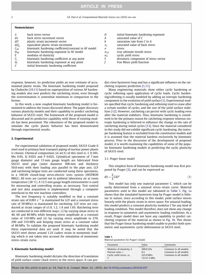
This model has only one material parameter C, which can beeasily determined from a uniaxial stress–strain curve. Materialparameters used in this model are tabulated in Table 1. Fig. 1ashows that the simulated hysteresis loop by Prager model is bilin-ear in nature, since according to this model, yield surface moveslinearly with the plastic strain in stress space. For uniaxial loading,this model predicts a constant plasticity modulus C for any kind ofloading condition. This model therefore, does not show any changein response in symmetric and asymmetric loading conditions. As aresult, Prager model does not have any capability to predict rat-cheting response of the material as shown in Fig. 1b. This showsthat the Prager linear hardening model unable to predict both sym-metric and asymmetric cyclic deformation in SA333 steel.

doi:10.1016/j.commatsci.2010.02.037

-2.0 -1.5 -1.0 -0.5 0.0 0.5 1.0 1.5 2.0-600

-400

-200

0

200

400

600

Experimental Prager

Stre

ss, M

Pa

Strain, %

(a)

(b)

0 5 10 15 20 25 300.0

0.5

1.0

1.5

2.0

Mean stress 60 MPaStress amplitude 310 MPa

Prager Experimental

Rat

chet

ing

stra

in, %

Number of cycles

Fig. 1. Prager model: (a) 1.6% LCF stable hysteresis loops and (b) ratcheting strainversus number of cycles at 60 MPa mean stress and 310 MPa stress amplitude.

Table 2Material parameters for Armstrong–Frederick’s model.

Parameter Value Comments

Modulus of elasticity, E 200.0 GPa Common to all modelsPoisson ratio, m 0.3 Common to all modelsCyclic yield stress, r0 225.0 MPa Common to all modelsCAF 41000.0 MPaDAF 200.0

S.K. Paul et al. / Computational Materials Science xxx (2010) xxx–xxx 3

ARTICLE IN PRESS

3.2. Multilinear model

First multiliear kinematic hardening model was proposed byMroz [4] as a multisurface model, where each surface representsa constant hardening modulus in the stress space. Besseling [6]introduced a multilayer model without any notion of surfaces.Also, Ohno and Wang (I) [7] introduced a piecewise linear kine-matic hardening model by means of superposition of several kine-matic hardening models which can be described as:

d�a ¼Xm

j¼1

daj

d�ai ¼23

Cjd�ep � Dj �aj dep ��aj

Fð�ajÞ

� �H �a2

j � ðCj=DjÞ2n o ð2Þ

where, H is Heaviside step function.In Ohno and Wang (I) model given above each decomposed

hardening model simulates a linear hardening with a slope Ci untilit reaches a critical value Ci/Di. In fact, all these models divide theuniaxial stress strain curve into many individual linear segments.When a sufficient number of segments are chosen, the simulationswould be close to experimentally determined hysteresis loops.Unfortunately, similar to linear kinematic hardening model, the

Please cite this article in press as: S.K. Paul et al., Comput. Mater. Sci. (2010),

multilinear models also predict a closed-loop when applied to auniaxial asymmetric stress cycle (with mean stress) and cloudnot portray uniaxial ratcheting [1,7]. Limitations of Ohno andWang (I) model were eliminated by introducing non-linearity[1,7] as follows:

d�aj ¼23

Cjd�ep � Dj �aj dep ��aj

Fð�ajÞ

� �Fð�ajÞCj=Dj

� �mi

ð3Þ

In this model, a minimum of 8–16 decomposition of stress–strain curve was proposed (i.e., 16–32 material constants). Rat-cheting strain accumulation in this modified model is entirelydepending on mi and number of decompositions [1].

3.3. Armstrong and Frederick (AF) model

Majority of the recently developed kinematic hardening models[10,14–21] are based on simple effective adjustments of initial AFkinematic hardening model. AF model can be described as:

d�a ¼ 23

CAFd�ep � DAF �adepeq ð4Þ

where, the equivalent plastic strain can be represented as:

depeq ¼

ffiffiffiffiffiffiffiffiffiffiffiffiffiffiffiffiffiffiffiffiffi23

d�ep � d�ep

rð5Þ

Integral form of Armstrong and Frederick model is

�a ¼ 23

CAF=DAFð Þ 1� e�DAF �adepeq

� �ð6Þ

CAF and DAF are determined from stable LCF hysteresis loop. In Arm-strong and Frederick model, the back stress is saturated at a value ofCAF/DAF. There are two terms in this model, one is the dynamicrecovery/recall term (DAF�adep

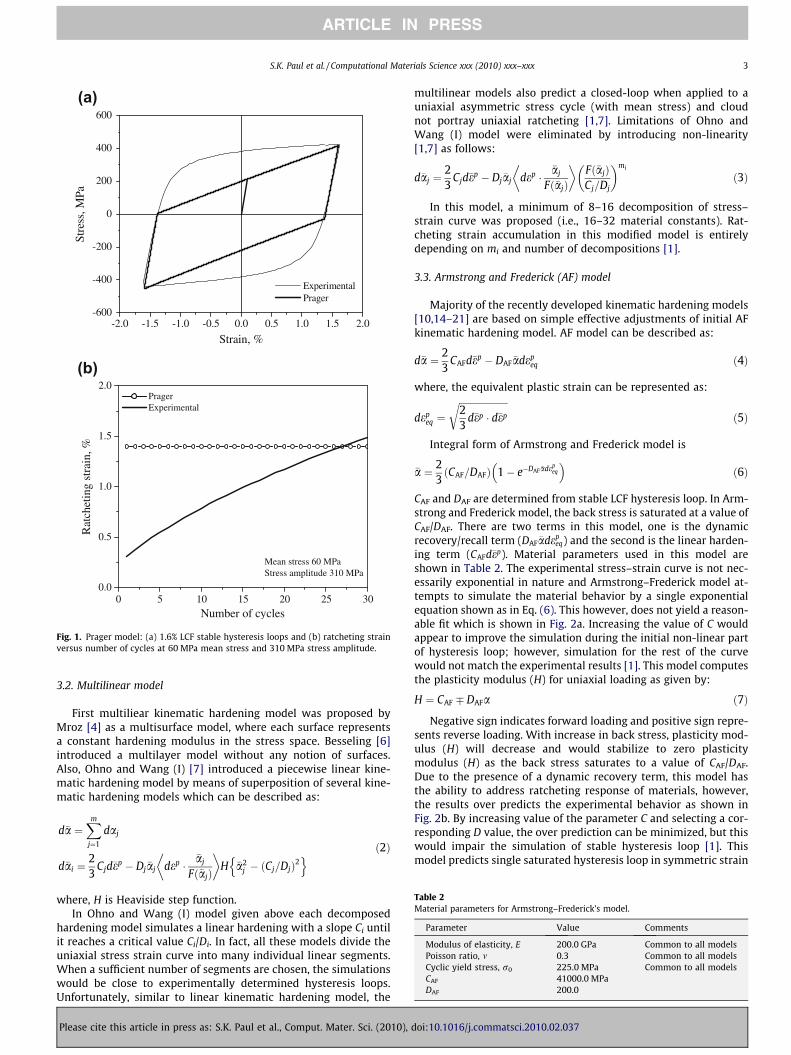
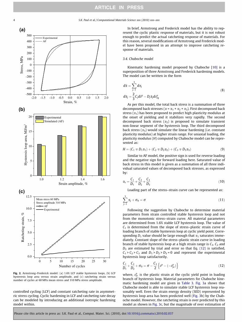
eq) and the second is the linear harden-ing term (CAFd�ep). Material parameters used in this model areshown in Table 2. The experimental stress–strain curve is not nec-essarily exponential in nature and Armstrong–Frederick model at-tempts to simulate the material behavior by a single exponentialequation shown as in Eq. (6). This however, does not yield a reason-able fit which is shown in Fig. 2a. Increasing the value of C wouldappear to improve the simulation during the initial non-linear partof hysteresis loop; however, simulation for the rest of the curvewould not match the experimental results [1]. This model computesthe plasticity modulus (H) for uniaxial loading as given by:

H ¼ CAF � DAFa ð7Þ

Negative sign indicates forward loading and positive sign repre-sents reverse loading. With increase in back stress, plasticity mod-ulus (H) will decrease and would stabilize to zero plasticitymodulus (H) as the back stress saturates to a value of CAF/DAF.Due to the presence of a dynamic recovery term, this model hasthe ability to address ratcheting response of materials, however,the results over predicts the experimental behavior as shown inFig. 2b. By increasing value of the parameter C and selecting a cor-responding D value, the over prediction can be minimized, but thiswould impair the simulation of stable hysteresis loop [1]. Thismodel predicts single saturated hysteresis loop in symmetric strain

doi:10.1016/j.commatsci.2010.02.037

-2.0 -1.5 -1.0 -0.5 0.0 0.5 1.0 1.5 2.0-500

-400

-300

-200

-100

0

100

200

300

400

500 Experimental AF

Stre

ss, M

Pa

Strain, %

(a)

1.0 1.2 1.4 1.60

5

10

15

20

Hys

tere

sis

loop

are

a, M

J/m

3

Strain amplitude, %

Experimental Simulated (AF)

(b)

(c)

0 5 10 15 20 25 30

0.0

2.5

5.0

7.5

10.0

12.5Mean stress 60 MPaStress amplitude 310 MPa

AF Experimental

Rat

chet

ing

stra

in, %

Number of cycles

Fig. 2. Armstrong–Frederick model: (a) 1.6% LCF stable hysteresis loops, (b) LCFhysteresis loop area versus strain amplitude, and (c) ratcheting strain versusnumber of cycles at 60 MPa mean stress and 310 MPa stress amplitude.

4 S.K. Paul et al. / Computational Materials Science xxx (2010) xxx–xxx

ARTICLE IN PRESS

controlled cycling (LCF) and constant ratcheting rate in asymmet-ric stress cycling. Cyclic hardening in LCF and ratcheting rate decaycan be modeled by introducing an additional isotropic hardeningmodel within.

Please cite this article in press as: S.K. Paul et al., Comput. Mater. Sci. (2010),

In brief, Armstrong and Frederick model has the ability to rep-resent the cyclic plastic response of materials, but it is not robustenough to predict the actual ratcheting response of materials. Forthis reason, several modifications of Armstrong and Frederick mod-el have been proposed in an attempt to improve ratcheting re-sponse of materials.

3.4. Chaboche model

Kinematic hardening model proposed by Chaboche [10] is asuperposition of three Armstrong and Frederick hardening models.The model can be written in the form

d�a ¼X3

j¼1

daj

d�aj ¼23

Cjd�ep � Dj �ajdepeq

ð8Þ

As per this model, the total back stress is a summation of threedecomposed back stresses (a = a1 + a2 + a3). First decomposed backstress (a1) has been proposed to predict high plasticity modulus atthe onset of yielding and it stabilizes very rapidly. The seconddecomposed back stress (a2) is proposed to simulate transientnon-linear segment of the hysteresis loop. The third decomposedback stress (a3) would simulate the linear hardening (i.e. constantplasticity modulus) at higher strain range. For uniaxial loading, theplasticity modulus (H) computed by Chaboche model can be repre-sented as:

H ¼ ðC1 � D1a1Þ þ ðC2 � D2a2Þ þ ðC3 � D3a3Þ ð9Þ

Similar to AF model, the positive sign is used for reverse loadingand the negative sign for forward loading here. Saturated value ofback stress in this model is given as a summation of all three indi-vidual saturated values of decomposed back stresses, as expressedby:

as ¼C1

D1þ C2

D2þ C3

D3ð10Þ

Loading part of the stress–strain curve can be represented as:

X3

j¼1

aj þ r0 ¼ r ð11Þ

Following the suggestion by Chaboche to determine materialparameters from strain controlled stable hysteresis loop and notfrom the monotonic stress–strain curve. All material parametersare determined from 1.6% stable LCF hysteresis loop. The value ofC1 is determined from the slope of stress–plastic strain curve ofloading branch of stable hysteresis loop at cyclic yield point. Corre-sponding D1 value should be large enough that a1 saturates imme-diately. Constant slope of the stress–plastic strain curve in loadingbranch of stable hysteresis loop at a high strain range is C3. C2 andD2 are estimated by trial and error so that Eq. (12) is satisfied,C1 > C2 > C3 and D1 > D2 > D3 = 0 and represent the experimentalhysteresis loop satisfactorily.

C1

D1þ C2

D2þ r0 ¼ r� C3

2ep � ð�ep

ycÞn o

ð12Þ

where, epyc is the plastic strain at the cyclic yield point in loading

branch of hysteresis loop. Material parameters for Chaboche kine-matic hardening model are given in Table 3. Fig. 3a shows thatChaboche model is able to simulate stable LCF hysteresis loop rea-sonably well. Even the strain energy density (SED) represented byhysteresis loop area has been predicted well (Fig. 3b) by the Chab-oche model. However, the ratcheting strain is over predicted by thismodel as shown in Fig. 3c, but the magnitude of over estimation of

doi:10.1016/j.commatsci.2010.02.037

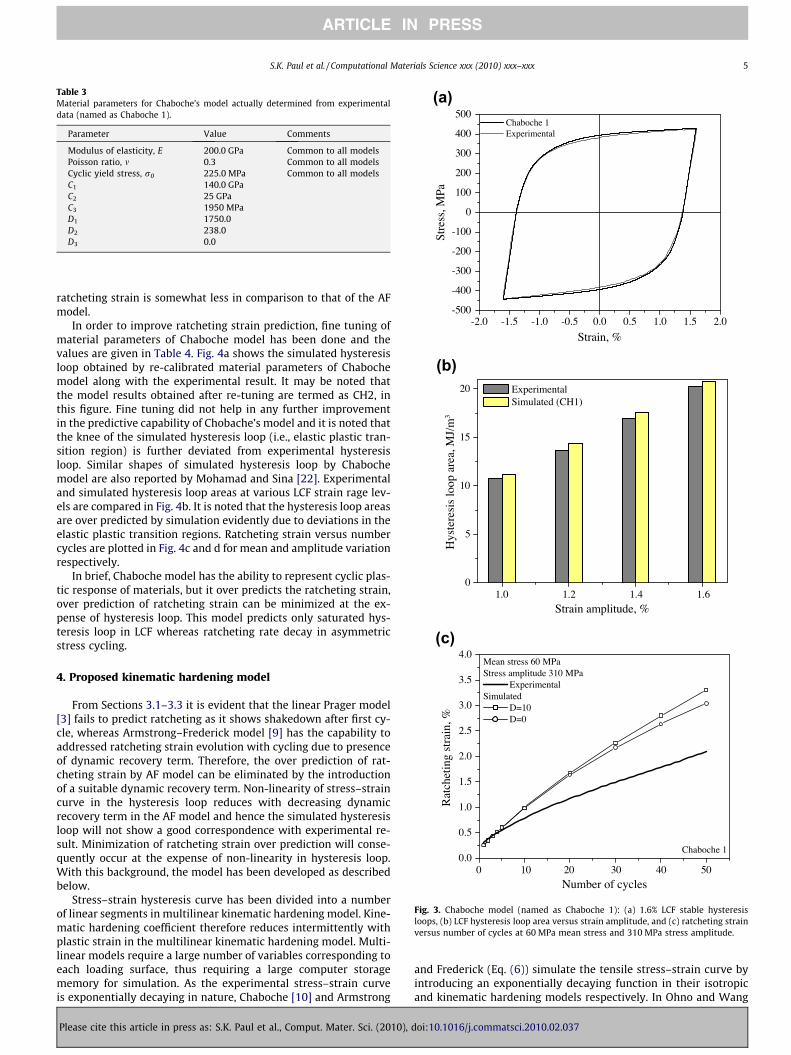
Table 3Material parameters for Chaboche’s model actually determined from experimentaldata (named as Chaboche 1).

Parameter Value Comments

Modulus of elasticity, E 200.0 GPa Common to all modelsPoisson ratio, m 0.3 Common to all modelsCyclic yield stress, r0 225.0 MPa Common to all modelsC1 140.0 GPaC2 25 GPaC3 1950 MPaD1 1750.0D2 238.0D3 0.0

-2.0 -1.5 -1.0 -0.5 0.0 0.5 1.0 1.5 2.0-500

-400

-300

-200

-100

0

100

200

300

400

500 Chaboche 1 Experimental

Stre

ss, M

Pa

Strain, %

(a)

1.0 1.2 1.4 1.60

5

10

15

20

Hys

tere

sis

loop

are

a, M

J/m

3

Strain amplitude, %

Experimental Simulated (CH1)

(b)

0 10 20 30 40 500.0

0.5

1.0

1.5

2.0

2.5

3.0

3.5

4.0

Chaboche 1

Mean stress 60 MPaStress amplitude 310 MPa

ExperimentalSimulated

D=10 D=0

Rat

chet

ing

stra

in, %

Number of cycles

(c)

Fig. 3. Chaboche model (named as Chaboche 1): (a) 1.6% LCF stable hysteresisloops, (b) LCF hysteresis loop area versus strain amplitude, and (c) ratcheting strainversus number of cycles at 60 MPa mean stress and 310 MPa stress amplitude.

S.K. Paul et al. / Computational Materials Science xxx (2010) xxx–xxx 5

ARTICLE IN PRESS

ratcheting strain is somewhat less in comparison to that of the AFmodel.

In order to improve ratcheting strain prediction, fine tuning ofmaterial parameters of Chaboche model has been done and thevalues are given in Table 4. Fig. 4a shows the simulated hysteresisloop obtained by re-calibrated material parameters of Chabochemodel along with the experimental result. It may be noted thatthe model results obtained after re-tuning are termed as CH2, inthis figure. Fine tuning did not help in any further improvementin the predictive capability of Chobache’s model and it is noted thatthe knee of the simulated hysteresis loop (i.e., elastic plastic tran-sition region) is further deviated from experimental hysteresisloop. Similar shapes of simulated hysteresis loop by Chabochemodel are also reported by Mohamad and Sina [22]. Experimentaland simulated hysteresis loop areas at various LCF strain rage lev-els are compared in Fig. 4b. It is noted that the hysteresis loop areasare over predicted by simulation evidently due to deviations in theelastic plastic transition regions. Ratcheting strain versus numbercycles are plotted in Fig. 4c and d for mean and amplitude variationrespectively.

In brief, Chaboche model has the ability to represent cyclic plas-tic response of materials, but it over predicts the ratcheting strain,over prediction of ratcheting strain can be minimized at the ex-pense of hysteresis loop. This model predicts only saturated hys-teresis loop in LCF whereas ratcheting rate decay in asymmetricstress cycling.

4. Proposed kinematic hardening model

From Sections 3.1–3.3 it is evident that the linear Prager model[3] fails to predict ratcheting as it shows shakedown after first cy-cle, whereas Armstrong–Frederick model [9] has the capability toaddressed ratcheting strain evolution with cycling due to presenceof dynamic recovery term. Therefore, the over prediction of rat-cheting strain by AF model can be eliminated by the introductionof a suitable dynamic recovery term. Non-linearity of stress–straincurve in the hysteresis loop reduces with decreasing dynamicrecovery term in the AF model and hence the simulated hysteresisloop will not show a good correspondence with experimental re-sult. Minimization of ratcheting strain over prediction will conse-quently occur at the expense of non-linearity in hysteresis loop.With this background, the model has been developed as describedbelow.

Stress–strain hysteresis curve has been divided into a numberof linear segments in multilinear kinematic hardening model. Kine-matic hardening coefficient therefore reduces intermittently withplastic strain in the multilinear kinematic hardening model. Multi-linear models require a large number of variables corresponding toeach loading surface, thus requiring a large computer storagememory for simulation. As the experimental stress–strain curveis exponentially decaying in nature, Chaboche [10] and Armstrong

Please cite this article in press as: S.K. Paul et al., Comput. Mater. Sci. (2010),

and Frederick (Eq. (6)) simulate the tensile stress–strain curve byintroducing an exponentially decaying function in their isotropicand kinematic hardening models respectively. In Ohno and Wang

doi:10.1016/j.commatsci.2010.02.037

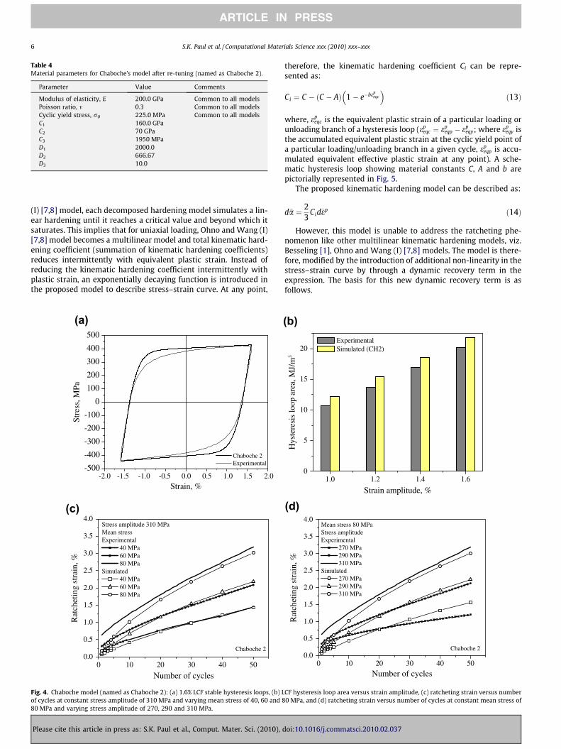
Table 4Material parameters for Chaboche’s model after re-tuning (named as Chaboche 2).

Parameter Value Comments

Modulus of elasticity, E 200.0 GPa Common to all modelsPoisson ratio, m 0.3 Common to all modelsCyclic yield stress, r0 225.0 MPa Common to all modelsC1 160.0 GPaC2 70 GPaC3 1950 MPaD1 2000.0D2 666.67D3 10.0

6 S.K. Paul et al. / Computational Materials Science xxx (2010) xxx–xxx

ARTICLE IN PRESS

(I) [7,8] model, each decomposed hardening model simulates a lin-ear hardening until it reaches a critical value and beyond which itsaturates. This implies that for uniaxial loading, Ohno and Wang (I)[7,8] model becomes a multilinear model and total kinematic hard-ening coefficient (summation of kinematic hardening coefficients)reduces intermittently with equivalent plastic strain. Instead ofreducing the kinematic hardening coefficient intermittently withplastic strain, an exponentially decaying function is introduced inthe proposed model to describe stress–strain curve. At any point,

-2.0 -1.5 -1.0 -0.5 0.0 0.5 1.0 1.5 2.0-500

-400

-300

-200

-100

0

100

200

300

400

500

Chaboche 2 Experimental

Stre

ss, M

Pa

Strain, %

(a)

(c)

0 10 20 30 40 500.0

0.5

1.0

1.5

2.0

2.5

3.0

3.5

4.0Stress amplitude 310 MPaMean stressExperimental

40 MPa 60 MPa 80 MPa

Simulated 40 MPa 60 MPa 80 MPa

Chaboche 2

Rat

chet

ing

stra

in, %

Number of cycles

Fig. 4. Chaboche model (named as Chaboche 2): (a) 1.6% LCF stable hysteresis loops, (b) Lof cycles at constant stress amplitude of 310 MPa and varying mean stress of 40, 60 and 880 MPa and varying stress amplitude of 270, 290 and 310 MPa.

Please cite this article in press as: S.K. Paul et al., Comput. Mater. Sci. (2010),

therefore, the kinematic hardening coefficient Ci can be repre-sented as:

Ci ¼ C � ðC � AÞ 1� e�bepeqc

� �ð13Þ

where, epeqc is the equivalent plastic strain of a particular loading or

unloading branch of a hysteresis loop (epeqc ¼ ep

eqp � epeqy; where ep

eqy isthe accumulated equivalent plastic strain at the cyclic yield point ofa particular loading/unloading branch in a given cycle, ep

eqp is accu-mulated equivalent effective plastic strain at any point). A sche-matic hysteresis loop showing material constants C, A and b arepictorially represented in Fig. 5.

The proposed kinematic hardening model can be described as:

d�a ¼ 23

Cid�ep ð14Þ

However, this model is unable to address the ratcheting phe-nomenon like other multilinear kinematic hardening models, viz.Besseling [1], Ohno and Wang (I) [7,8] models. The model is there-fore, modified by the introduction of additional non-linearity in thestress–strain curve by through a dynamic recovery term in theexpression. The basis for this new dynamic recovery term is asfollows.

1.0 1.2 1.4 1.60

5

10

15

20

Hys

tere

sis

loop

are

a, M

J/m

3

Strain amplitude, %

Experimental Simulated (CH2)

(b)

(d)

0 10 20 30 40 500.0

0.5

1.0

1.5

2.0

2.5

3.0

3.5

4.0Mean stress 80 MPaStress amplitudeExperimental

270 MPa 290 MPa 310 MPa

Simulated 270 MPa 290 MPa 310 MPa

Chaboche 2

Rat

chet

ing

stra

in, %

Number of cycles

CF hysteresis loop area versus strain amplitude, (c) ratcheting strain versus number0 MPa, and (d) ratcheting strain versus number of cycles at constant mean stress of

doi:10.1016/j.commatsci.2010.02.037

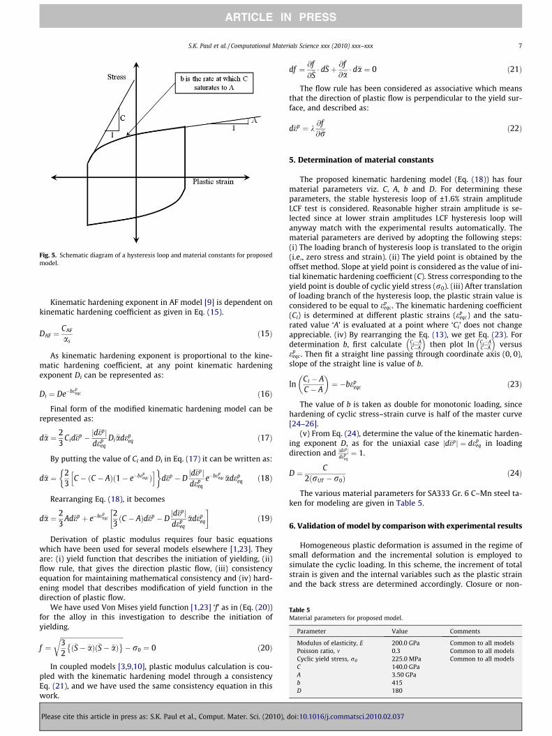
Fig. 5. Schematic diagram of a hysteresis loop and material constants for proposedmodel.

Table 5Material parameters for proposed model.

Parameter Value Comments

Modulus of elasticity, E 200.0 GPa Common to all modelsPoisson ratio, m 0.3 Common to all modelsCyclic yield stress, r0 225.0 MPa Common to all modelsC 140.0 GPaA 3.50 GPab 415D 180

S.K. Paul et al. / Computational Materials Science xxx (2010) xxx–xxx 7

ARTICLE IN PRESS

Kinematic hardening exponent in AF model [9] is dependent onkinematic hardening coefficient as given in Eq. (15).

DAF ¼CAF

asð15Þ

As kinematic hardening exponent is proportional to the kine-matic hardening coefficient, at any point kinematic hardeningexponent Di can be represented as:

Di ¼ De�bepeqc ð16Þ

Final form of the modified kinematic hardening model can berepresented as:

d�a ¼ 23

Cid�ep � jd�epj

depeq

Di �adepeq ð17Þ

By putting the value of Ci and Di in Eq. (17) it can be written as:

d�a ¼ 23

C � ðC � AÞð1� e�bepeqc Þ

h i d�ep � D

jd�epjdep

eqe�bep

eqc �adepeq ð18Þ

Rearranging Eq. (18), it becomes

d�a ¼ 23

Ad�ep þ e�bepeqc

23ðC � AÞd�ep � D

jd�epjdep

eq

�adepeq

� �ð19Þ

Derivation of plastic modulus requires four basic equationswhich have been used for several models elsewhere [1,23]. Theyare: (i) yield function that describes the initiation of yielding, (ii)flow rule, that gives the direction plastic flow, (iii) consistencyequation for maintaining mathematical consistency and (iv) hard-ening model that describes modification of yield function in thedirection of plastic flow.

We have used Von Mises yield function [1,23] ‘f’ as in (Eq. (20))for the alloy in this investigation to describe the initiation ofyielding.

f ¼ffiffiffiffiffiffiffiffiffiffiffiffiffiffiffiffiffiffiffiffiffiffiffiffiffiffiffiffiffiffiffiffiffiffiffiffiffiffiffi32ð�S� �aÞð�S� �aÞ �r

� r0 ¼ 0 ð20Þ

In coupled models [3,9,10], plastic modulus calculation is cou-pled with the kinematic hardening model through a consistencyEq. (21), and we have used the same consistency equation in thiswork.

Please cite this article in press as: S.K. Paul et al., Comput. Mater. Sci. (2010),

df ¼ @f@�S� d�Sþ @f

@�a� d�a ¼ 0 ð21Þ

The flow rule has been considered as associative which meansthat the direction of plastic flow is perpendicular to the yield sur-face, and described as:

d�ep ¼ k@f@�r

ð22Þ

5. Determination of material constants

The proposed kinematic hardening model (Eq. (18)) has fourmaterial parameters viz. C, A, b and D. For determining theseparameters, the stable hysteresis loop of ±1.6% strain amplitudeLCF test is considered. Reasonable higher strain amplitude is se-lected since at lower strain amplitudes LCF hysteresis loop willanyway match with the experimental results automatically. Thematerial parameters are derived by adopting the following steps:(i) The loading branch of hysteresis loop is translated to the origin(i.e., zero stress and strain). (ii) The yield point is obtained by theoffset method. Slope at yield point is considered as the value of ini-tial kinematic hardening coefficient (C). Stress corresponding to theyield point is double of cyclic yield stress (r0). (iii) After translationof loading branch of the hysteresis loop, the plastic strain value isconsidered to be equal to ep

eqc. The kinematic hardening coefficient(Ci) is determined at different plastic strains (ep

eqc) and the satu-rated value ‘A’ is evaluated at a point where ‘Ci’ does not changeappreciable. (iv) By rearranging the Eq. (13), we get Eq. (23). Fordetermination b, first calculate Ci�A

C�A

� �then plot ln Ci�A

C�A

� �versus

epeqc . Then fit a straight line passing through coordinate axis (0, 0),

slope of the straight line is value of b.

lnCi � AC � A

� �¼ �bep

eqc ð23Þ

The value of b is taken as double for monotonic loading, sincehardening of cyclic stress–strain curve is half of the master curve[24–26].

(v) From Eq. (24), determine the value of the kinematic harden-ing exponent D, as for the uniaxial case jd�epj ¼ dep

eq in loadingdirection and jd�ep j

depeq¼ 1.

D ¼ C2ðrUT � r0Þ

ð24Þ

The various material parameters for SA333 Gr. 6 C–Mn steel ta-ken for modeling are given in Table 5.

6. Validation of model by comparison with experimental results

Homogeneous plastic deformation is assumed in the regime ofsmall deformation and the incremental solution is employed tosimulate the cyclic loading. In this scheme, the increment of totalstrain is given and the internal variables such as the plastic strainand the back stress are determined accordingly. Closure or non-

doi:10.1016/j.commatsci.2010.02.037

8 S.K. Paul et al. / Computational Materials Science xxx (2010) xxx–xxx

ARTICLE IN PRESS

closure of the hysteresis loop depends upon path of the load appli-cation. For symmetric loading (i.e. LCF, stress controlled fatigue atzero mean stress) hysteresis loop will completely close and forasymmetric loading (i.e. ratcheting) hysteresis loop will remainopen, resulting in a gradual accumulation of strain. Partiallyopened hysteresis loop arises due to the presence of non-zeromean stress since difference exists in the plasticity modulus of ten-sile and compressive branches [27]. Recall term in AF model (Eq.(4)) is responsible for the creation of difference in the plasticitymodulus during fluctuating loading and hence the ratcheting strain[1,2]. Multilinear kinematic hardening models [6–8] are incapableto explain this creation of difference in the plasticity modulus dur-ing asymmetric load reversal, as a result, predict a closed hystere-sis loop. In the proposed model, an attempt has been made toremove the over prediction of ratcheting strain by minimizingthe difference in plasticity modulus during asymmetric alternatingloading, i.e. reducing recall term without sacrificing the non-linear-ity of hysteresis loop, using a exponentially decaying kinematichardening coefficient. Variation in cyclic yield stress can also leadto a measurable difference in the ratcheting strain [14,27] due tovariation of back stress evolution. It must be noted that the totalstress is the summation of cyclic yield stress and back stress anddynamic recovery term is a function of back stress. Therefore,low cyclic yield stress would lead to a high back stress and high dy-namic recovery term which in turn would result in a large ratchet-ing strain.

(b)

0 2 4 6 8 10 120.00

0.25

0.50

0.75

1.00

1.25

1.50

1.75

2.00

Stress amplitude 310 MPaMean stress 80 MPa

C 140 GPa C 120 GPa

Rat

chet

ing

Stra

in, %

Number of Cycles

(a)

-2.0 -1.5 -1.0 -0.5 0.0 0.5 1.0 1.5 2.0-600

-400

-200

0

200

400

600Stress amplitude 310 MPaMean stress 80 MPa

C 120 GPa C 140 GPa

Stre

ss, M

Pa

Total strain, %

Fig. 6. Effect of parameter C in LCF loop and ratcheting strain.

Please cite this article in press as: S.K. Paul et al., Comput. Mater. Sci. (2010),

The proposed model is validated by verifying and comparingthe simulated and experimental results for symmetric loadingand that of the asymmetric loading. For precise simulation ofexperimental results, it is essential to tune the parameters C, Dand b appropriately.

By selecting b and C values equal to zero, the proposed kine-matic hardening model (Eq. (18)) becomes the AF model [9] foruniaxial case. On the other hand, for uniaxial case, if C, b and D val-ues becomes zero, the proposed model becomes the Prager’s model[3].

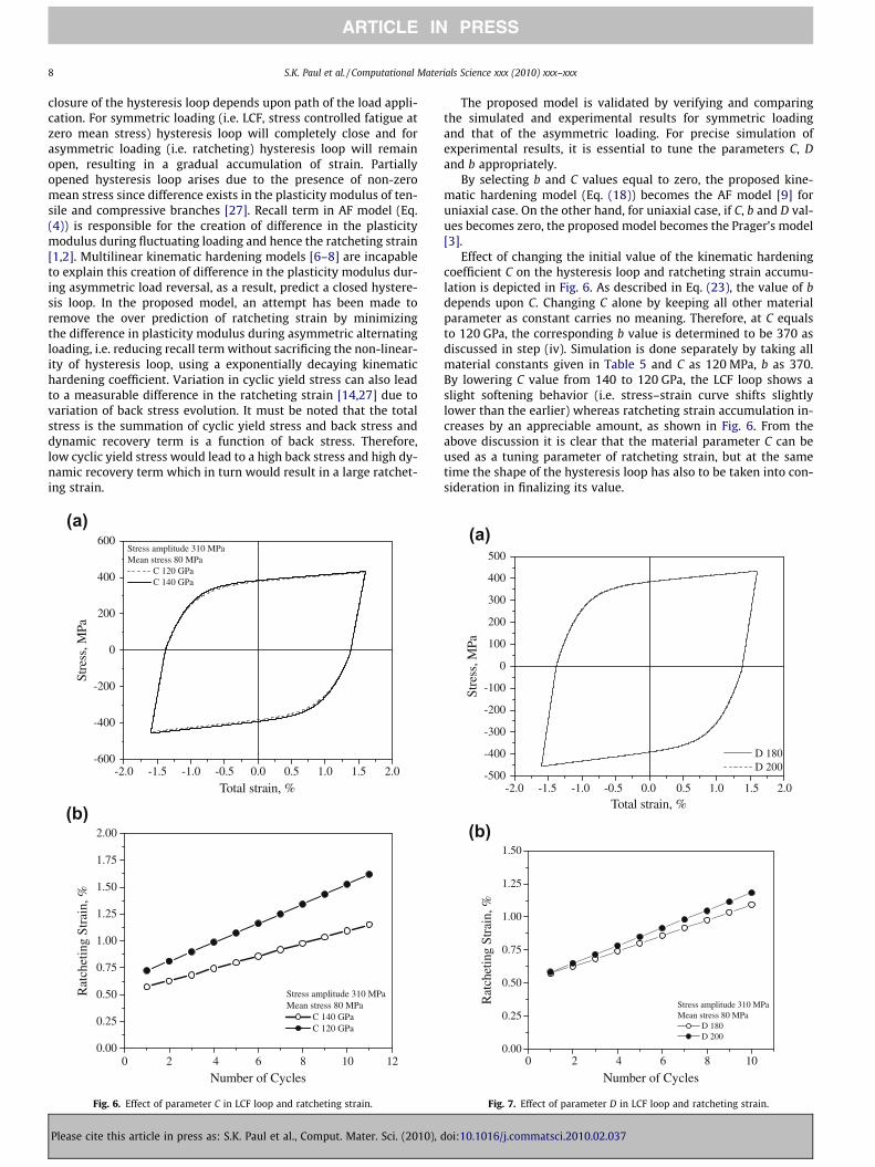
Effect of changing the initial value of the kinematic hardeningcoefficient C on the hysteresis loop and ratcheting strain accumu-lation is depicted in Fig. 6. As described in Eq. (23), the value of bdepends upon C. Changing C alone by keeping all other materialparameter as constant carries no meaning. Therefore, at C equalsto 120 GPa, the corresponding b value is determined to be 370 asdiscussed in step (iv). Simulation is done separately by taking allmaterial constants given in Table 5 and C as 120 MPa, b as 370.By lowering C value from 140 to 120 GPa, the LCF loop shows aslight softening behavior (i.e. stress–strain curve shifts slightlylower than the earlier) whereas ratcheting strain accumulation in-creases by an appreciable amount, as shown in Fig. 6. From theabove discussion it is clear that the material parameter C can beused as a tuning parameter of ratcheting strain, but at the sametime the shape of the hysteresis loop has also to be taken into con-sideration in finalizing its value.

-2.0 -1.5 -1.0 -0.5 0.0 0.5 1.0 1.5 2.0-500

-400

-300

-200

-100

0

100

200

300

400

500

D 180 D 200

Stre

ss, M

Pa

Total strain, %

0 2 4 6 8 100.00

0.25

0.50

0.75

1.00

1.25

1.50

Stress amplitude 310 MPaMean stress 80 MPa

D 180 D 200

Rat

chet

ing

Stra

in, %

Number of Cycles

(a)

(b)

Fig. 7. Effect of parameter D in LCF loop and ratcheting strain.

doi:10.1016/j.commatsci.2010.02.037

-2.0 -1.5 -1.0 -0.5 0.0 0.5 1.0 1.5 2.0-600

-400

-200

0

200

400

600

Experimental Simulated

Stre

ss, M

Pa

Total strain, %

(a)

-500

-400

-300

-200

-100

0

100

200

300

400

500

Experimental Simulated

Stre

ss, M

Pa

(c)

-1.25 -1.00 -0.75 -0.50 -0.25 0.00 0.25 0.50 0.75 1.00 1.25-500

-400

-300

-200

-100

0

100

200

300

400

500

Experimental Simulated

Stre

ss, M

Pa

Total Strain, %

(d)

-1.5 -1.0 -0.5 0.0 0.5 1.0 1.5

Total Strain, %

-1.5 -1.0 -0.5 0.0 0.5 1.0 1.5-500

-400

-300

-200

-100

0

100

200

300

400

500

Experimental Simulated

Stre

ss, M

Pa

Total Strain, %

(b)

Fig. 8. Comparison between experimental and simulated stable LCF hysteresis loops at strain amplitude of (a) 1.0, (b) 1.2, (c) 1.4, and (d) 1.6%.

0.9 1.0 1.1 1.2 1.3 1.4 1.5 1.6 1.7-10

-5

0

5

10

15

Armstrong - Frederick Chaboche 1 Chaboche 2 Proposed

Err

or in

hys

tere

sis

loop

are

a pr

edic

tion

, %

Strain amplitude, %

Fig. 9. Error in hysteresis loop area prediction by different models with LCF strainrange.

S.K. Paul et al. / Computational Materials Science xxx (2010) xxx–xxx 9

ARTICLE IN PRESS

As pointed out earlier, the matching of simulated ratchetingstrain with experimental results can be achieved by decreasingthe dynamic recovery term DAF in the AF model which also affectsthe non-linearity of the hysteresis loop. In the AF model, the non-linearity of stress–strain curve appears solely from the dynamicrecovery term. However the non-linearity of stress–strain curvein the proposed model arises from the exponential decay of kine-matic hardening coefficient. Dynamic recovery term inserts anadditional non-linearity in the stress–strain curve in the proposedmodel and its contribution is minimal in comparison to the decay-ing kinematic hardening coefficient. Therefore the effect of non-linearity on stress–strain curve by decrement of kinematic harden-ing exponent in the proposed model is not as prominent as in AFmodel. By increasing D value from 180 to 200 and keeping all othermaterial parameters (as specified in Table 1) constant, the shape ofLCF hysteresis loop does not change noticeably, where as the rat-cheting strain accumulation increases by substantial amount, asdepicted in Fig. 7. So the parameter D can be used efficiently as afinal tuning parameter to match the ratcheting strain accumulationwith the experimental results.

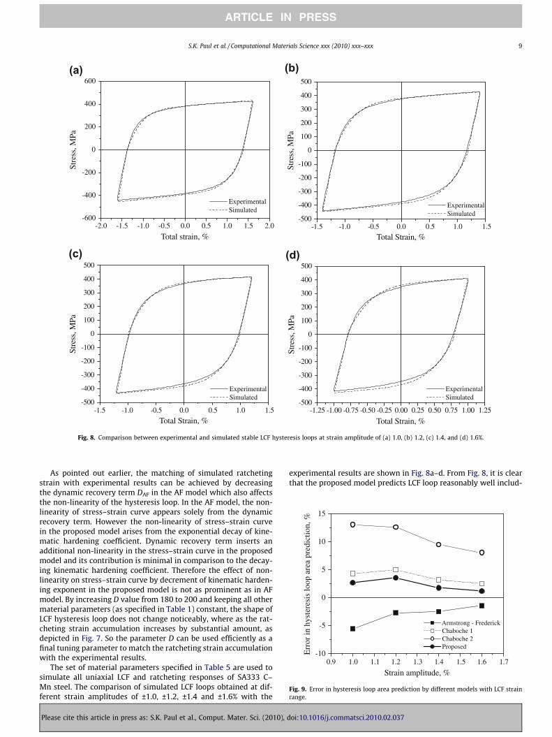
The set of material parameters specified in Table 5 are used tosimulate all uniaxial LCF and ratcheting responses of SA333 C–Mn steel. The comparison of simulated LCF loops obtained at dif-ferent strain amplitudes of ±1.0, ±1.2, ±1.4 and ±1.6% with the

Please cite this article in press as: S.K. Paul et al., Comput. Mater. Sci. (2010),

experimental results are shown in Fig. 8a–d. From Fig. 8, it is clearthat the proposed model predicts LCF loop reasonably well includ-

doi:10.1016/j.commatsci.2010.02.037

(a)

0 10 20 30 40 500.0

0.5

1.0

1.5

2.0

2.5

3.0

3.5

4.0Stress amplitude 310 MPaMean stressExperimental

40 MPa 60 MPa 80 MPa

Simulated 40 MPa 60 MPa 80 MPa

Proposed model

Rat

chet

ing

stra

in. %

Number of cycles

(b)

0.0

0.5

1.0

1.5

2.0

2.5

3.0

3.5

4.0Mean stress 80 MPaStress amplitudeExperimental

270 MPa 290 MPa 310 MPa

Simulated 270 MPa 290 MPa 310 MPa

Proposed model

Rat

chet

ing

stra

in, %

Number of cycles0 10 20 30 40 50

Fig. 10. Comparison between experimental and simulated ratcheting strain accu-mulation (a) at constant stress amplitude of 310 MPa and mean stress of 40 MPa,60 MPa and 80 MPa and (b) at constant mean stress of 80 MPa and stress amplitudeof 270 MPa, 290 MPa and 310 MPa.

10 S.K. Paul et al. / Computational Materials Science xxx (2010) xxx–xxx

ARTICLE IN PRESS

ing the elastic–plastic transition region. It provides an addedadvantage over the Chaboche’s model (shown in Fig. 4a) whichcould not simulate the transition regions accurately. Errors in thehysteresis loop area prediction by different models are shown inFig. 9 for comparing the predictive capability of the proposed mod-el. This figure clearly demonstrated that the best prediction of hys-teresis loop is possible by the proposed model.

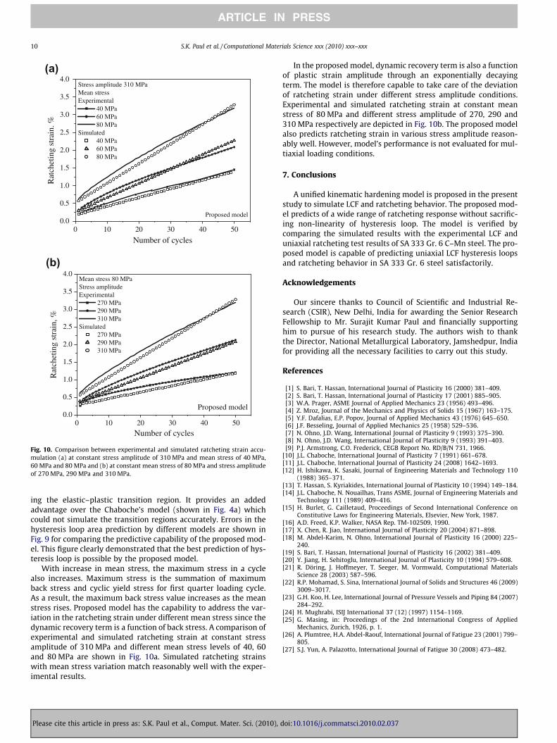
With increase in mean stress, the maximum stress in a cyclealso increases. Maximum stress is the summation of maximumback stress and cyclic yield stress for first quarter loading cycle.As a result, the maximum back stress value increases as the meanstress rises. Proposed model has the capability to address the var-iation in the ratcheting strain under different mean stress since thedynamic recovery term is a function of back stress. A comparison ofexperimental and simulated ratcheting strain at constant stressamplitude of 310 MPa and different mean stress levels of 40, 60and 80 MPa are shown in Fig. 10a. Simulated ratcheting strainswith mean stress variation match reasonably well with the exper-imental results.

Please cite this article in press as: S.K. Paul et al., Comput. Mater. Sci. (2010),

In the proposed model, dynamic recovery term is also a functionof plastic strain amplitude through an exponentially decayingterm. The model is therefore capable to take care of the deviationof ratcheting strain under different stress amplitude conditions.Experimental and simulated ratcheting strain at constant meanstress of 80 MPa and different stress amplitude of 270, 290 and310 MPa respectively are depicted in Fig. 10b. The proposed modelalso predicts ratcheting strain in various stress amplitude reason-ably well. However, model’s performance is not evaluated for mul-tiaxial loading conditions.

7. Conclusions

A unified kinematic hardening model is proposed in the presentstudy to simulate LCF and ratcheting behavior. The proposed mod-el predicts of a wide range of ratcheting response without sacrific-ing non-linearity of hysteresis loop. The model is verified bycomparing the simulated results with the experimental LCF anduniaxial ratcheting test results of SA 333 Gr. 6 C–Mn steel. The pro-posed model is capable of predicting uniaxial LCF hysteresis loopsand ratcheting behavior in SA 333 Gr. 6 steel satisfactorily.

Acknowledgements

Our sincere thanks to Council of Scientific and Industrial Re-search (CSIR), New Delhi, India for awarding the Senior ResearchFellowship to Mr. Surajit Kumar Paul and financially supportinghim to pursue of his research study. The authors wish to thankthe Director, National Metallurgical Laboratory, Jamshedpur, Indiafor providing all the necessary facilities to carry out this study.

References

[1] S. Bari, T. Hassan, International Journal of Plasticity 16 (2000) 381–409.[2] S. Bari, T. Hassan, International Journal of Plasticity 17 (2001) 885–905.[3] W.A. Prager, ASME Journal of Applied Mechanics 23 (1956) 493–496.[4] Z. Mroz, Journal of the Mechanics and Physics of Solids 15 (1967) 163–175.[5] Y.F. Dafalias, E.P. Popov, Journal of Applied Mechanics 43 (1976) 645–650.[6] J.F. Besseling, Journal of Applied Mechanics 25 (1958) 529–536.[7] N. Ohno, J.D. Wang, International Journal of Plasticity 9 (1993) 375–390.[8] N. Ohno, J.D. Wang, International Journal of Plasticity 9 (1993) 391–403.[9] P.J. Armstrong, C.O. Frederick, CEGB Report No. RD/B/N 731, 1966.

[10] J.L. Chaboche, International Journal of Plasticity 7 (1991) 661–678.[11] J.L. Chaboche, International Journal of Plasticity 24 (2008) 1642–1693.[12] H. Ishikawa, K. Sasaki, Journal of Engineering Materials and Technology 110

(1988) 365–371.[13] T. Hassan, S. Kyriakides, International Journal of Plasticity 10 (1994) 149–184.[14] J.L. Chaboche, N. Nouailhas, Trans ASME, Journal of Engineering Materials and

Technology 111 (1989) 409–416.[15] H. Burlet, G. Cailletaud, Proceedings of Second International Conference on

Constitutive Laws for Engineering Materials, Elsevier, New York, 1987.[16] A.D. Freed, K.P. Walker, NASA Rep. TM-102509, 1990.[17] X. Chen, R. Jiao, International Journal of Plasticity 20 (2004) 871–898.[18] M. Abdel-Karim, N. Ohno, International Journal of Plasticity 16 (2000) 225–

240.[19] S. Bari, T. Hassan, International Journal of Plasticity 16 (2002) 381–409.[20] Y. Jiang, H. Sehitoglu, International Journal of Plasticity 10 (1994) 579–608.[21] R. Döring, J. Hoffmeyer, T. Seeger, M. Vormwald, Computational Materials

Science 28 (2003) 587–596.[22] R.P. Mohamad, S. Sina, International Journal of Solids and Structures 46 (2009)

3009–3017.[23] G.H. Koo, H. Lee, International Journal of Pressure Vessels and Piping 84 (2007)

284–292.[24] H. Mughrabi, ISIJ International 37 (12) (1997) 1154–1169.[25] G. Masing, in: Proceedings of the 2nd International Congress of Applied

Mechanics, Zurich, 1926, p. 1.[26] A. Plumtree, H.A. Abdel-Raouf, International Journal of Fatigue 23 (2001) 799–

805.[27] S.J. Yun, A. Palazotto, International Journal of Fatigue 30 (2008) 473–482.

doi:10.1016/j.commatsci.2010.02.037