Simulation of an urban battery bus vehicle : final report

REPORT NO. UMT A- MA -06-0093-79-1

p&

HF

nni-TSr-i

!

k q/\-79- ic;

SIMULATION OF AN URBAN BATTERY BUS VEHICLE

John J . Stickler

U.S. DEPARTMENT OF TRANSPORTATIONRESEARCH AND SPECIAL PROGRAMS ADMINISTRATION

Trans portati on Systems CenterCambridge MA 02142

JULY 1979

DEPARTMENT OFTRANSPORTATION

MflV 1 1979

n

LIBRARY

FINAL REPORT

DOCUMENT IS AVAILABLE TO THE PUBLICTHROUGH THE NATIONAL TECHNICALINFORMATION SERVICE, SPRINGFIELD.VIRGINIA 22161

f 9

3

Prepared for

,U.S. DEPARTMENT OF TRANSPORTATIONURBAN MAS^TRANSPORTATION ADMINISTRATION

Office of Technology Development and DeploymentWashington DC 20590

NOTICE

This document is disseminated under the sponsorshipof the Department of Transportation in the interestof information exchange. The United States Govern-ment assumes no liability for its contents or usethereof

.

NOTICE

The United States Government does not endorse pro-ducts or manufacturers. Trade or manufacturers'names appear herein solely because they are con-sidered essential to the object of this report.

Technical Report Documentation Page

3. Recipient's Catalog No.

Vt

?.r

kinno,

rs c-1 . Report No.

UMTA -MA -06-0093-79-12. Government Accession No.

'I-/«

4. Title ond Subtitle

SIMULATION OF AN URBAN BATTERY BUS VEHICLE

7. Author's)

5. Report Date

July 19796. Performing Organization Code

8. Performing Organization Report No.

John J. Stickler DOT- TSC - UMTA- 79-15

9. Performing Organization Name and Address

U.S. Department of TransportationResearch and Special Programs AdministrationTransportation Systems CenterCambridge MA 02142

10. Work Unit No. (TRAIS)

UM946/R972911. Contract or Grant No.

13. Type of Report ond Period Covered

Final ReportJune-Dee. 1978

12. Sponsoring Agency Name and Address

U.S. Department of TransportationUrban Mass Transportation AdministrationOffice of Technology Development § DeploymentWashington DC 20590

14. Sponsoring Agency Code

15. Supplementary Notes

16. Abstract

1

This report describes the computer simulation of a battery-poweredbus as it traverses an arbitrary mission profile of specified accelera-tion, roadway grade, and headwind. The battery-bus system componentscomprise a DC shunt motor, solid-state power conditioning unit withregeneration capability, and a battery source consisting of a multi-unit lead acid battery. The computer model determines vehicle tractiveeffort and power consumption and computes actual vehicle speed for a

given mission profile. The program output data is tabulated in a formwhich allows easy recognition of the various operational modes andpower- limited regimes.

The computer model uses a "modularization" format which facilitatesthe simulation of alternate propulsion systems involving the interchangeof one system component for another. The mod gj is applied to simulatethe propulsion characteristics of a typical bps ope lU ling ov-wa; a

specified drive cycle. The results of this s!tU(P^dB^M£NTTaftejthe appli-

cability of the battery bus model for predictfin^^NfifQWTO^^i P n charac-teristics under simulated drive conditions.

| |

NOV 1 1979

library17. Key Words 18. Dlitribution feijtement

Battery Bus Simulation,Battery Bus PropulsionCharacteristics

DOCUMENT iS AVAILABLE lO i lit PUBl.lC

THROUGH THt NATIONAL TECHNICALINFORMATION SERVICE, SPRINGFIELD.VIRGINIA 2216 1

19. Security Clo.tlf. (of (hit report) 20. Security Clpttif. (of thl» page) 21* No. of Pages 22. Price

Unc lass i f ied Unclassified 90

Form DOT F 1700.7 (8-72) Reproduction of completed page authorized

i

PREFACE

This report describes a computer model of a battery-powered

bus developed at the Transportation Systems Center to simulate

the power/propulsion characteristics of an urban battery-bus. This

model comprises the third in a series of models being developed at

TSC to simulate different types of bus propulsion systems. These

simulation models provide the capability for rapid evaluation of

bus performance through the comparison of simulated bus performance

with data obtained from engineering tests. The work conducted in

this area is sponsored by the Urban Mass Transportation Administra-

tion and is part of a larger effort concerned with the demonstration

and test evaluation of advanced bus propulsion concepts.

i i i

im

i !rlE iVi § £ 3 - -:U>tl

OUu

S

I«s

ao

S

<*«_ i4*

Ve~E 5 S

i 11 I

§ | f |

tillitn.

mil i ?

. r . 5 *

s i I? f

fiillllll

«s>

Iiiis IIIs

~3

tiE> £ * > e s'iV E 3 S ill 6. S'

TABLE OF CONTENTS

Section Page

1. INTRODUCTION 1

1.1 Background Discussion 1

1.2 Simulation Description 2

1.3 Modularized Program Format 3

1.4 Simulation Approach 6

1.5 Performance Criteria for Electric - BatteryDrive 7

2. BASELINE SYSTEM: COMPONENTS AND MODES OF OPERATION. 8

2.1 Configuration of Major Components 8

2.1.1 Vehicle Bus 8

2.1.2 Battery Power Bank 8

2.1.3 DC Traction Motor 132.1.4 Power Control Unit (PCU) 17

2.2 Modes of Operation 192.3 Mission Profile 23

3. MODELING THEORY AND EQUATIONS 28

3.1 Mission Profile Model 283 . 2 Motor Model 323.3 PCU Model 363.4 Battery Model 37

4. PROGRAM OPERATION 43

4.1 Executing the Program 454.2 Plotting Program CHART. FOR 46

5. APPLICATION OF COMPUTER PROGRAM TO BATTERY BUSOPERATION 47

5.1 FORTRAN Source Listings and Data Files 535.2 Battery Bus Performance Program 65

APPENDIX - GLOSSARY OF PROGRAM CONSTANTS ANDVARIABLES 73

REFERENCES 81

v

LIST OF ILLUSTRATIONS

Figure Page

1-1 BLOCK DIAGRAM OF BATTERY BUS PROPULSION SYSTEM 3

1-

2 SIMPLIFIED FLOWCHART ILLUSTRATING MODULARIZATIONPROGRAM FORMAT 5

2-

la BATTERY CAPACITY AS A FUNCTION OF DISCHARGECURRENT 10

2- lb BATTERY VOLTAGE AS A FUNCTION OF PERCENT DISCHARGE 10

2-2 CHARGING CHARACTERISTICS FOR BATTERY CELL 12

2-3 TRACTION MOTOR SHUNT FIELD LOSS 14

2-4 EXCITATION CONSTANT AS A FUNCTION OF MOTORSPEED FOR DRIVE CYCLE C 18

2 - 5a PCU VOLTAGE STEP-DOWN CIRCUIT 20

2 - 5b PCU VOLTAGE STEP-UP CIRCUIT.......... 20

2 - 6a POWER FLOW IN MOTORING MODE 21

2 - 6b POWER FLOW IN BRAKING MODE 21

2 - 7a SPEED-TIME PROFILE CHARACTERISTIC 24

2 - 7b ACCELERATION - (DECELERATION) TIME PROFILE 24

4-

1 PROGRAM FLOWCHART 44

5-

la CALCOMP Plots of System Parameters - DrivingCycle A. 48

5- lb CALCOMP Plots of System Parameters - DrivingCycle B . . . 49

LIST OF TABLES

Table Page

2-1 SUMMARY OF BATTERY BUS PARAMETERS 9

2-2 BATTERY CELL CHARACTERISTICS 9

2-3 LEAD-ACID BATTERY CELL DISCHARGE DATA 11

2-4 DC TRACTION MOTOR RATINGS 13

2-5 DC MOTOR POWER LOSSES AT RATED SPEED.. 15

2-6 MAXIMUM TRACTION MOTOR RATINGS 15

2-

7 DRIVING CYCLE DATA 2 6

3-

1 SUMMARY OF TRACTION MOTOR DATA 33

5-1 COMPUTER INPUT DATA 50*

vii

EXECUTIVE SUMMARY

This report describes a computer model of a battery-powered

bus developed at the Transportation Systems Center to simulate

power/propulsion characteristics of an urban battery-bus. This

model comprises the third in a series of models being developed

at TSC to simulate different types of bus propulsion systems. The

work conducted in this area is sponsored by the Urban Mass Trans-

portation Administration as part of a larger effort concerned with

the demonstration and test evaluation of advanced bus propulsion

concepts. The computer models developed by TSC provide the capa-

bility for rapid evaluation of bus performances and the comparison

of simulated bus performance with that obtained from engineering

tests. Such studies give important insights into the limitations

inherent in the different propulsion systems and permit rapid

assessments to be made of the future practicality of such systems.

Current efforts in other areas of bus propulsion simulation

include the (1) cam-controlled trolley bus, (2) pure flywheel bus,

(3) flywheel/battery hybrid bus, and (4) the flywheel/diesel hybrid

bus with electric transmission. Studies have already been

completed on the diesel engine model and the results documented in

the reports, "Flywheel/Diesel Hybrid Power Drive: Urban Bus

Vehicle Simulation," May 1978 by Larson and Zuckerberg;"^ "Diesel

Bus Performance Simulation Program," April 1979 by Larson and?

Zuckerberg. Upon the completion of these simulation studies,

TSC will possess the capability of simulating a wide range of bus

propulsion systems. Such capability should prove extremely useful

in future evaluations and analyses of urban bus systems.

Larson, G.S. and H. Zuckerberg, Flywheel/Diesel Hybrid PowerDrive : Urban Bus Vehicle Simulation , U . S. Department of Transpor-tation, Urban Mass Transportation Administration, Washington DC,Final Report, UMTA-MA- 0 6- 0 044 - 7 8

- 1 ,May 1978.

2Larson G. and H. Zuckerberg, Diesel Bus Performance SimulationProgram , U.S. Department of Transportation, Urban Mass Transporta-tion Administration, Washington DC, Final Report, UMTA-MA- 06- 0044-79-1, April 1979.

vi i i

1. INTRODUCTION

1.1 BACKGROUND DISCUSSION

The development of battery-powered vehicles has progressed

rapidly with the aid of advances in battery and lightweight vehicle

technology. New improvements in vehicle design, battery con-

struction, and motor controllers have resulted in reduced vehicle

weight and drag as well as increased vehicle speed and range

capabilities. While the present performance and economy of bat-

tery-powered vehicles cannot match that of internal combustion-

powered vehicles, the trend towards minimizing environmental pol-

lution increases the desirability of electric-powered vehicles.

When compared with conventional vehicles, electric vehicles are

extremely quiet and waste less energy at idle.

Research and development are now being conducted on numerous

electric drive configurations. These include propulsion systems

using flywheels for energy storage and hybrid systems using both

batteries and flywheels for energy storage. A major program in

bus propulsion technology is presently being sponsored jointly by

the U.S. Department of Transportation and the U.S. Department of

Energy. This program calls for the test evaluation and demonstra-

tion of two engineering prototype vehicles, one propelled by fly-

wheel only, and the second propelled by a diesel/flywheel hybrid.

The General Electric Company and the Garrett Airesearch Corpora-

tion are the prime contractors for these respective vehicle-

propulsion technology programs.

The Transportation Systems Center at Cambridge, Massachusetts

is conducting simulation studies of different bus propulsion

systems anticipated in future urban bus transport systems. This

report, which describes the simulation of a battery-powered bus,

comprises one phase of this study. Two TSC reports have been

published to date by Larson and Zuckerberg: " Flywheel/ Dies el

Hybrid Power Drive : Urban Bus Vehicle Simulation," Final Report ,

May 1978 and "Diesel Bus Performance Simulation Program," Final

Report,April 1979. Additional efforts are in progress now

1

to model other bus propulsion systems, including the cam-controlled

trolley bus, battery/flywheel hybrid, and the flywheel/diesel

hybrid. These models will be used eventually by both government

and industry to aid in the preliminary assessment of the compara-

tive performances of the different bus propulsion systems.

This report discusses the computer model developed to simulate

a battery bus as it travels over a prescribed speed-time mission

profile. The model is constructed of separate functional units

referred to as a modularized format to simplify the logic in the

program calculations as well as to make it easily adaptable to

changes in the propulsion system components. The flexibility

achieved through the use of this format increases the usefulness

of the battery bus model both as a design tool and as an instrument

for evaluating alternate types of bus propulsion systems.

1.2 SIMULATION DESCRIPTION

The computer program described in this report models a battery-

powered vehicle as it traverses a defined mission profile of

acceleration, cruising speed, roadway grade, and headwind. The

vehicle acceleration (deceleration) and cruise velocity-versus-time

requirements determine the propulsion power required by the vehicle.

For a given mission profile, the vehicle power consumption is

computed as output data. The power - 1 imit ing regions and system

losses, which characterize the motor and battery, are easily

identifiable from the output data.

The program describes a propulsion system comprising a battery

source, dc traction motor, and a power conditioning unit (PCU)

for the control of motor power. (See Figure 1-1.) A separately

excited dc shunt motor was selected to be modeled because it gives

relatively constant tractive effort while allowing easy speed

control. Motor speed is voltage-controlled except at high speeds

where field-weakening is required.

2

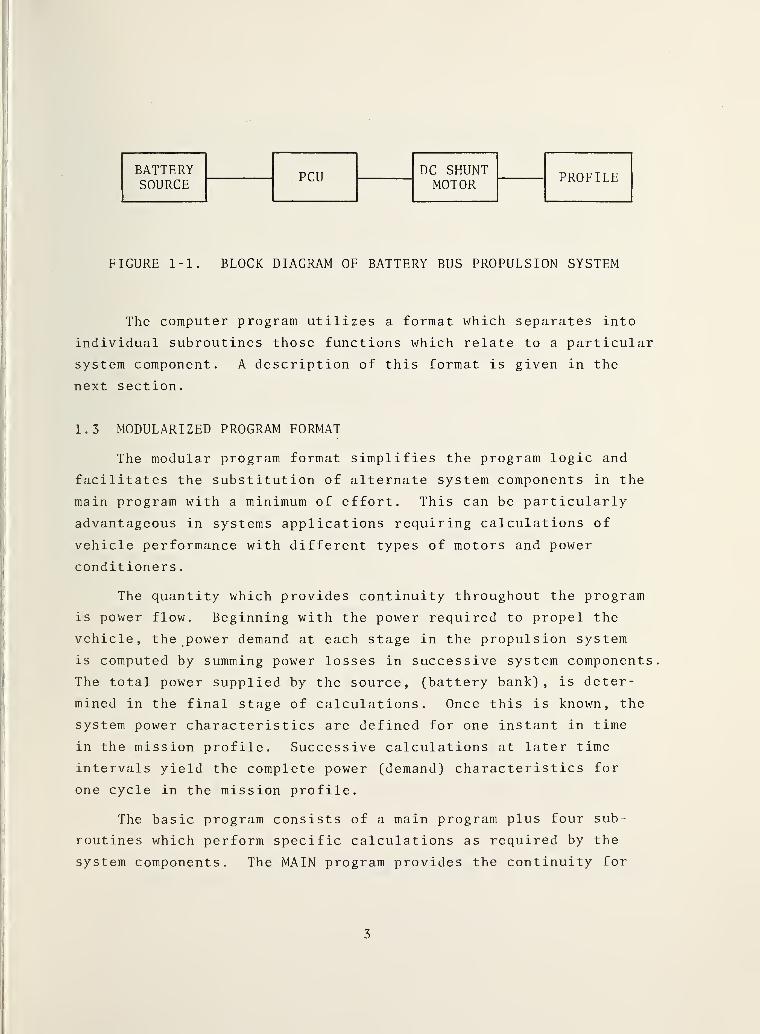
FIGURE 1-1. BLOCK DIAGRAM OF BATTERY BUS PROPULSION SYSTEM

The computer program utilizes a format which separates into

individual subroutines those functions which relate to a particular

system component. A description of this format is given in the

next section.

1.3 MODULARIZED PROGRAM FORMAT

The modular program format simplifies the program logic and

facilitates the substitution of alternate system components in the

main program with a minimum of effort. This can be particularly

advantageous in systems applications requiring calculations of

vehicle performance with different types of motors and power

conditioners

.

The quantity which provides continuity throughout the program

is power flow. Beginning with the power required to propel the

vehicle, the power demand at each stage in the propulsion system

is computed by summing power losses in successive system components.

The total power supplied by the source, (battery bank), is deter-

mined in the final stage of calculations. Once this is known, the

system power characteristics are defined for one instant in time

in the mission profile. Successive calculations at later time

intervals yield the complete power (demand) characteristics for

one cycle in the mission profile.

The basic program consists of a main program plus four sub-

routines which perform specific calculations as required by the

system components. The MAIN program provides the continuity for

3

the ongoing successive calculations as well as program logic and

CALL statements. A simplified flowchart illustrating the modular-

ized concept is shown in Figure 1-2. The program execution begins

with the MAIN program, followed by the subroutines PROF, MOTOR,

PCU, and BATT,which describe the mission profile, motor, and bat-

tery respectively. The quantities at the left give the power

required at each stage in the propulsion system; the quantities

at the right indicate the input-output parameters associated with

each subroutine. A more complete flowchart appears later in the

report

.

The subroutines contain the operating characteristics of each

system component. Subroutine PROF computes the mission profile at

successive time iterations. Included in the profile are vehicle

acceleration and speed, position of the vehicle, roadway grade, and

encountered headwind.

The subroutine MOTOR receives the request for the required

tractive effort at a specified vehicle speed and computes the motor

losses and total electrical input power required by the traction

motor. The motor terminal voltage (VOLT) and armature current (AMP)

are determined and appear as output quantities of subroutine MOTOR.

The subroutine PCU computes the power loss in the SCR chopper

circuit and determines the total power required by the battery

(minus the auxiliary power).

The subroutine BATT models the charge and discharge character-

istics of a water-cooled lead-acid battery*. The modeling equations

assume a constant discharge-charge rate, with the battery capacity

being equal to that obtained at the constant discharge rate. ^ The

battery current required to satisfy the output power demands is

computed via the Newton- Raphson method. The battery is assumed to

be discharged when it has delivered 60 percent of its rated (five

hour) capacity.

4 '

*This battery is manufactured in West Germany.

4

PowerRequirements

InputParameters

OutputParameters

P = t-Vm

Pag

E •

a

P =Vmut t ^ *pf

P + Pniut pcu

(Accel ,Vcruise )

(Thrust , V)

^ P BAT ’ IBAT'*

(Thrust ,V)

(Vt,I

1,PF)

^ P BAT ’ 11

-1

*-VBAT ’ 1

BAT-*

KEY

P =Mechanical Powerm

P =Airgap Powerag 6 H

P = Motor Input Powermut ^

P = PCU Input Powerpcu ^

Prat= Battery Output Power

FIGURE 1-2. SIMPLIFIED FLOWCHART ILLUSTRATING MODULARIZATIONPROGRAM FORMAT

5

1.4 SIMULATION APPROACH

The computer program calculates the dynamic behavior of the

vehicle as it travels over the prescribed profile route. Using

as input the cruise velocity, the specified acceleration and

deceleration plus their respective jerk-rate limits, and the

distance between route stops, the program computes the speed-time

profile at successive instants in time. This is followed by the

calculation of the drive system powers, e.g., propulsion power,

system power losses, and required battery power. The battery power

and discharge current are summed (over time) to yield the total

instantaneous energy and charge extracted from the battery.

The computer program includes regeneration in which the

kinetic energy of the moving vehicle is converted into electrical

power delivered to the battery. Constraints are introduced to

limit the amount of regenerated power which the battery can

accept. The increase in drive-cycle efficiency due to regenera-

tion is easily determined from the computer output data.

The power control unit (PCU) is modeled as a chopper- flyback

circuit with the capability of power transfer in either direction

between source and load. Power transfer is assumed to take place

irrespective of the voltage levels of the source and load com-

ponents (i.e., power transfer can include a voltage step-up or step

down)

.

The battery source is modeled by an equivalent circuit com-

prising a fixed resistance (temperature dependent) and a load

dependent resistance which is a function of the discharge current

level and battery capacity. The battery capacity is expressed as

a function of discharge current. Separate models are used to de-

scribe the battery discharge and charge characteristics. The

models include the loss associated with the reduction in the charge

delivered to the battery compared with that delivered by battery

to load.

6

1.5 PERFORMANCE CRITERIA FOR ELECTRIC-BATTERY DRIVE

The computer program can be used to optimize the system com-

ponents and to compute the battery, PCU,and motor losses for dif-

ferent drive conditions. This information is useful for establish-

ing performance criteria and for sizing the various system com-

ponents .

The computer program is designed to simulate different drive

cycles and thereby study effects associated with the type of drive

cycle as it relates to propulsion performance. The so-called A,

B, and C drive cycles which describe idealized speed-time profiles

are used to establish baseline criteria for typical mission pro-

files. The program has the additional capability of simulating

arbitrary drive cycles which conform to prescribed cruise velocity

and acceleration (deceleration) conditions.

Two factors are important in determining drive efficiency;

(1) the proper rating of the major system components, and (2) the

ability of the battery supply to meet the required energy and power

demands. The ratings selected for the major components determine

how heavily they are loaded in use. Too low a rating results in

overloading and less efficient operation (higher power losses) .

Too large a rating introduces a penalty associated with increased

size, weight, and cost of the system. The specifications of the

battery size (capacity) is dictated by the ratings of commercially

available batteries. The significant criteria, in this case, is

battery energy density (energy/weight) and the ability of the bat-

tery to deliver large peak power. The total distance which the

vehicle traverses between periods of battery recharging will be

determined by the rating of the battery bank supply.

7

2 , BASELINE SYSTEM: COMPONENTS AND MODES OF OPERATION

2.1 CONFIGURATION OF MAJOR COMPONENTS

The battery vehicle computer program simulates the power and

propulsion characteristics of any generalized vehicle powered by a

dc source. For purposes of analysis, a set of baseline system

parameters were used in the simulation model. The values of these

parameters which define the battery source, power controller, and

dc traction motor, were chosen to be compatible with system com-

ponents presently available. They do not represent the ultimate

choice in terms of overall system efficiency. Advances in vehicle

technology and battery development will likely yield better vehicle

performance in the future than is predicted by the vehicle simula-

tion program. The following sections describe the vehicle components

used in the battery bus model.

2.1.1 Vehicle Bus

The vehicle chosen for simulation is a rubber-tired bus of

approximately 18 tons weight, capable of accommodating 20 pas-

sengers plus the operator of the bus. On-board the vehicle is

auxilliary equipment for supplying the necessary lighting as well

as air-conditioning. Table 2-1 gives a summary of the bus param-

eters used in the battery bus simulation.

2.1.2 Battery Power Bank

The power source is modeled as a multiple battery cell com-

prising a total of 256 cells which has a charge capacity of 455

ampere-hours. Total energy capacity of the unit is 910 watt-hours.

A summary of pertinent battery data is presented in Table 2-2.

Figure 2-la shows the charge capacity as a function of dis-

charge current. Intercepts on the curve give the expected

ampere-hours output for different discharge times

8

TABLE 2-1. SUMMARY OF BATTERY BUS PARAMETERS

Bus Parameters

Curb Weight 36,400 lb

No. of Passengers (150 lb each) 20

Gross Vehicle Weight 39 ,550 lb

Frontal Area 80 sq ft

Aerodynamic Drag Coeff. . 84

Rolling Drag Coeff. . 005

Airconditioning Compressor Power 6 kw

Aircompressor Load 1 kw

Airconditioning Condenser . 6 kwBlower Power

Environmental Control Blower . 6 kw

TABLE 2-2. BATTERY CELL CHARACTERISTICS

5 Hour Discharge Rate

Cell Voltage 1.96 vDischarge Current 91 ampCapacity 455 AHEnergy Storage 910 WhEnergy/Weight Ratio 31.4 Wh/kg

1 Hour Discharge Rate

Cell Voltage 1.86 v.Discharge Current 315 ampCapacity 315 AHEnergy Storage 630 Wh (nom inal

)

Energy/Weight Ratio 21.7 Wh/kg****************************************************************’.•*

Weight 29 kgMaximum Discharge Current 600 amp

9

630

FIGURE 2 -lb. BATTERY VOLTAGE AS A FUNCTION OF PERCENT DISCHARGE

10

with continuous discharge current. The corresponding cell output

voltage as a function of percent of total ampere-hours output is

shown in Figure 2-lb. The reduction in cell capacity and output

voltage at high discharge current levels is evident in the

figures

.

The discharge current I, average discharge voltage U,and

final discharge voltage Us

are given in Table 2-3.

TABLE 2-3. LEAD-ACID BATTERY CELL DISCHARGE DATA

Hr C I U IJ

m s

AH A V V

10 518 52 .

0

1.955 1 .735

5 455 91 1 .935 1 . 715

3 409.5 136.5 1.92 1.70

2 377.0 187.0 1 .90 1.78

1 315 315 1.855 1.635

1/2 255 .5 511 1 . 785 1.565

1/4 203 812 1.67 1.46

The charging current characteristics for the lead-acid

cell follow the typical charging characteristics for lead acid

storage batteries. Figure 2-2 presents charging voltage as a

function of charging current for various states of battery charge

relative to the ampere-hour capacity at the 10 hour-rate level,

i.e., 518 A-h. Onset of gassing occurs at 2.4 volts per cell.

The figure shows that charging current must be progressively

reduced as the state-of -charge of the battery builds up to avoid

battery gassing.

11

CHARGING

VOLTAGE,

VOLTS/CELL

2.9

FIGURE 2-2. CHARGING CHARACTERISTICS FOR BATTERY CELL.(ABSCISSA SHOULD BE MULTIPLIED BY 5.18 FOR ACTUALCHARGING CURRENT).

12

2.1.3 DC Traction Motor

The battery bus uses a separately excited dc shunt motor,

which is coupled through a gear box with 11.42 gear ratio (step

down) to the rear drive axle of the vehicle. The motor character-

istics at rated output are listed in Table 2-4.

TABLE 2-4. DC TRACTION MOTOR RATINGS

Shunt (separately excited)

Rated Speed 2,477 rpm

Power Output (continuous) 300 HP (323 kw)

Armature Current (rated load) 478 amp

Terminal Voltage (rated load) 530 volt

Rated Efficiency (field loss andblower power loss omitted)

92 %

The motor losses depend on its speed and the relative motor

excitation. The parameter, k, equal to (airgap) vol ts -per- rpm

describes the motor excitation. The losses are assumed to be

given by the following relations:

1) Iron Loss. The iron loss depends on both the motor speed

and excitation. The loss is assumed to be given by

the empirical relation,

P. = 2.629x10 (k)^ ^ (rpm)

^^ kw.iron

2) Bearing Loss. The bearing loss is proportional to motor

speed

,

P, . = O.OOlx(rpm) kw.bearing r

3) Windage Loss. The windage power loss varies as the

square of the motor speed,

P . ,= 1 . 4 7 5x (rpm/4 540

)^ •

windage r

13

24) Primary I R Heating Loss. Primary resistance is taken to

be .0405 ohm .

5) Shunt Field Loss. The shunt field loss as a function of

field excitation (volt /rpm) is shown in Figure 2-3.

FIGURE 2-3. TRACTION MOTOR SHUNT FIELD LOSS

14

Below an excitation level of 0.18 volt /rpm, the field loss

is described by a function involving the 5.65 power; above the

excitation level of 0.18, field loss is given by the square of the

excitation. Table 2-5 gives the motor losses for an assumed

excitation of Kq

equal to 0.215 (volt /rpm).

TABLE 2-5. DC MOTOR POWER LOSSES AT RATED SPEED

DC MOTOR POWER LOSSES*

Iron Loss 2.14 kw

Bearing Loss 2.48 kw

Windage Loss 0.41 kw

Field Power Loss see Figure 2-3

*Assumed excitation = 0.215 volt /rpm

The limiting conditions assumed for the dc traction motor are

summarized in the table below.

TABLE 2-6. MAXIMUM TRACTION MOTOR RATINGS

MAXIMUM MOTOR RATINGS

Armature Current = 700 amperes

Terminal Voltage = 530 volt

Field Excitation = 0.215 volt /rpm

Field Excitation = 0.230 volt /rpm

(motoring)

(braking)

Motor Excitation . The motor excitation which determines the

field (flux) in the dc motor is described by the input (airgap)

volts per motor rpm. Since the machine flux results from both

the field and armature windings both excitations must be con-

sidered in determining the effective motor excitation.

15

At low motor speeds, the motor back EMF is small and the

terminal voltage must be reduced to limit armature current. The

motor operates with maximum (field) excitation which is limited

by the current through the field winding. The excitation k,

in

this case, is given by,

where

ko

Ea_

rpm ( 1 )

V.

V,

vt

- VB

- 12*R (2)

motor terminal voltage

brush voltage drop = 2 volts

armature current

armature resistance = 0.04 ohm .

The field (current) excitation k is set at 0.215 for the DCo

traction motor. The armature current 1^ is determined by the

motor output power, or equivalently, the airgap power PTMA.

I1

PTMA(3)

This assumes the armature current does not exceed the maximum

allowed current AMPM. If 1^ given by Equation (3) exceeds AMPM,

the motor output power must be reduced to satisfy Equation (3).

The required motor terminal voltage V^. for this f ield - 1 imited

mode is (see Section 3.2),

V = kQ

* rpm + Vg + PTMA * R/ (KQ*rpm) . (4)

As the motor speeds up, the back EMF Ea

increases and the

motor terminal voltage rises. When the motor speed becomes such

that the terminal voltage equals the maximum available voltage.

16

in thisVOLTM, the motor is voltage-limited. The excitation,

case, is

E

ka

v rpm *

and (see Section 3.2)

VOLTMEa 2

4 PTMA • R. (5)

The armature current given by Equation (3) must not exceed the

maximum allowed current AMPM;otherwise the output power must be

reduced to satisfy Equation (3)

.

Figure 2-4 shows the motor excitation volts/rpm for the dc

traction motor computed for Drive Cycle C (see Section 5). The

figure illustrates the field and voltage- 1 imited operating regimes.

In the voltage- limited regime, field-weakening is required to

reach higher speeds.

Motor operation in the regenerative braking mode requires an

increase in field excitation to develop the necessary EMF for re-

versing the armature current. (See Equation (2) ). For this purpose

the motor excitation is assigned a value k = .230 volt /rpm which

is sufficient at high rpm's to cause the back EMF to exceed the

motor terminal voltage. Regenerative braking is possible at all

speeds for which the above condition exists.

2.1.4 Power Control Unit (PCU)

Power delivered by the battery source to the dc traction

motor is controlled by a solid state unit consisting of a step-down

chopper and a step-up (boost PCU) circuitry. By utilizing the

b i- funct ional capability of the step down, step up dc to dc con-

verters, it is possible with a single control unit to transfer

power between the battery source and motor during both the motoring

and regenerative braking modes. Without the voltage step—up

capability, regenerative power transfer at the lower motor speed

17

Ph

E-i

—1O>

<HCOSOuSOi—

i

E-*

<Hi—

i

UXw

. 5

. 4

. 3

. 2

. 1

0

\

\

\

\

FIELDLIMITED

\\

VOLTAGELIMITED

0 10 20 30

MOTOR SPEED - RPM40

FIGURE 2-4. EXCITATION CONSTANT AS A FUNCTION OF MOTOR SPEED

FOR DRIVE CYCLE C

18

range would be impossible and the propulsion system efficiency

would be reduced. This type of control unit envisioned is

3described in the literature as a dc to dc converter and in-

corporates a flyback booster and chopper regulator.

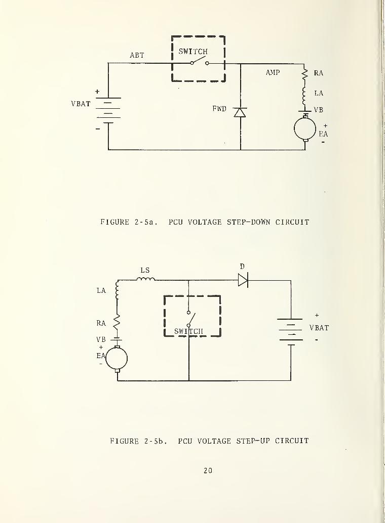
The control circuit is shown in its most simplified form in

Figure 2-5a and 2-5b which describe respectively step-down and

step-up (voltage) converters. The step-down converter utilizes

SCR to periodically connect the power source to the load. A free-

wheeling diode, FWD,provides the current continuity as required by

the large inductance in the motor circuit. Output voltage is given

by the time-average of the chopped voltage output signal.

Voltage step up is illustrated by the circuit shown in

Figure 2-5b. Closing the SCR switch causes a large voltage to be

developed across the inductance (LS) . When the switch is opened,

this voltage, plus additional induced voltages in the circuit

(motor EMF),are placed in series with the battery. The series

diode prevents battery discharge when the switch is closed.

Reference 4 describes the operation of the step-up converter in

more detail

.

2.2 MODES OF OPERATION

The propulsion system of the battery bus operates in both the

motoring and regenerative braking modes. In the former, power flow

is from the battery source to the dc traction motor; in the lat-

ter, the motor acts as a generator and supplies power to the bat-

tery bank. In both operating modes, power losses exist in the

different system components. These losses determine the ultimate

efficiency of the bus propulsion system when operating with a

given drive cycle.

The two operating modes are best illustrated by the diagrams

shown in Figures 2-6a and 2-6b. The direction of power flow in

the figures is indicated by arrows. The symbols used for the

various loss terms are those used in the battery bus program.

19

VBAT

FIGURE 2 -5a. PCU VOLTAGE STEP-DOWN CIRCUIT

VBAT

FIGURE 2- 5b. PCU VOLTAGE STEP-UP CIRCUIT

(Auxiliary

Power)

PAUX

u

+-* Pi f—

'

pi o3 Eh

> PCPP CD

k +-* o is

H p P om.O 2 Pc

PC

COPh

i

wQI—

I

PhoPiPh

> MW•K a3 co

Q Eh OHQP

<SE—1

Pc

tafl^-* CD /—

s

i ifl mvih t/) a3 to

Eh o Q otup iPCD -HCP 3=

l-H CP2 2H E—1

Ph PhHPh

<iSE—1

PiCSl

,

PC2<

PiOE—1

O2

CO

CO

oQPi

CXJ

2E-1

PC

CPPh

a3 ixP Eh PiP CD /—

n

WCD +-> in HM +-> co HPi 03 O <

l—

l

CP Q CP

+->

o3

Q

HQO

ox;I—

I

Pioo

oQpp

PiwisoPc

aj

vO

Q in 1

Pi Q co Q CXI

QUO UPC PC Q PC W

PiQCOI—

I

pH

w

o• iH

P /—

'

P cfl pP5 PP CD

> PU ?* p m o

> bO in

x o3 co

P P OH Q Q

oHP

Pi

oS-H

tao co 0 co

P3 co tao co

•H O a3 OP C T3 PIaj (p

CD -HCP X

He CP2 2E—

iE-i

PC PhHPC

E—i 0)

Pi Eh

cxi 3/-N +->

PC 03

co

moQ

e ccEh On!

' < I—

I

Q in

Pi Q inQUOPc PC Q

Eh

CD

is

oPC

XX QEh <a3 PC

•H

•Hx

<

a3 XP Eh

Eh CD i—

>

<D +-> in

•P> +-> C/1

P 03 Oh m p

p>aj

Q•K

ow

21

FIGURE

2-

6b.

POWER

FLOW

IN

BRAKING

MODE

Certain limitations in the flow of power to and from the bat-

tery exist which are not detailed in the figure. First, the bat-

tery is limited in the total current it can discharge. This affects

the maximum power which the battery is capable of delivering.

Second, the battery is limited in the amount of current it can

accept during charging. Exceeding this limit results in battery

gassing and subsequent deterioration in the chemical structure of

the battery. The latter limit is referred to as gassing power

limit. Both of these limits have an important effect on the maximum

power output and efficiency of the battery.

The limiting conditions for bus operation in the motoring mode

are

:

1) Battery discharge current is limited to ABM = 422

amperes

.

2) Motor armature current is limited to AMPMO = 700 amperes.

3 ) Motor terminal voltage is limited to VOLTMA = 530 volt .

4 ) Motor terminal voltage (VOLT) cannot exceed battery

voltage (VBAT)

.

5) Field excitation is limited to rated excitation defined

by CAYOA = 0.215 volt / rpm in the speed- voltage control

mode

.

Condition 1 above limits the maximum acceleration at the

higher speed range while condition 4 defines the limiting condition

for field weakening.

The limiting conditions for bus operation in the regenerative

braking mode are:

a) Maximum charging power of the battery bank is limited

to the gassing power PG. The gassing power is the battery

power corresponding to a gassing voltage EG = 2.4 volt /

cell

.

b) Motor terminal voltage is limited to VOLTMD = 600 volts.

c) The field excitation is limited to the excitation constant

value of CAYOD = 0.23 volt/rpm.

22

d) The battery has a charging efficiency of 90 p ercent as

determined by the ratio of the actual charge stored to the

total charge delivered to the battery.

2.3 MISSION PROFILE

The mission profile de scribes the position and sp eed of the

vehicle at any given time. Usually the mission prof il e is a

specified function of speed and time which the vehicle undergoes

in operation. An alternate arrangement consists of requesting a

desired vehicle acceleration and cruise velocity and allowing the

vehicle to achieve a speed-time profile compatible with the re-

quested acceleration and velocity input data. The latter arrange-

ment corresponds to the one experienced in normal vehicle opera-

tion. Other considerations such as roadway grade and headwind are

usually defined as part of the mission profile since they affect

the required tractive effort needed to achieve a given vehicle

acceleration or speed.

The battery bus program uses the alternate arrangement de-

scribed above in determining the mission profile. Figure 2-7a

shows the drive cycle used to describe the vehicle mission profile

over an operat ing " interval . " Figure 2-7b shows the vehicle

acceleration, cruise velocity, and deceleration subject to limiting

acceleration and deceleration jerk rates. The parameters required

to define the vehicle drive cycle are:

VC = Cruise speed

ACCM = Requested acceleration

DECL = Requested deceleration

Dwell = Time spent at station stop

T1 = Time interval of initial deceleration

T2-T1 = Time interval for cons tant decelera

T3-T2 = Time interval of final decel erat ion

AJERKR = Jerk rate.

23

FIGURE 2-1 di. SPEED-TIME PROFILE CHARACTERISTIC

ACCmph/sec

FIGURE 2 - 7b . ACCELERATION- (DECELERATION) TIME PROFILE

24

The total vehicle route comprises a multiple of driving cycles

in which the vehicle stops at successive stations for a period of

time (DWELL) . The relevant parameters which describe the vehicle

route are;

NS = Number of stops per mile

SR = Route length.

The possibility of different waiting periods between routes is in-

cluded in the program.

TAUMU = Waiting time between routes.

Additional parameters needed to describe the roadway grade and head-

wind are;

GRADE = Roadway grade

HW = Headwind.

The mission profile is described by selecting one of three

programmed driving cycles, A, B, and C. The cycles are defined by

the constants given in Table 2-7.

The vehicle starts from rest in a jerk-limited mode. As the

acceleration (ACC) increases to the required rate (ACCM),the jerk

(AJERK),which is the rate of change of acceleration, is constrained

by a specified limit (AJERKR) . As the vehicle approaches cruise

speed (VC), a jerk-limited decrease of acceleration is programmed.

At the proper speed, the acceleration is reduced to zero at the

jerk-limited rate (AJERKR) so that cruise speed is maintained at,

or slightly above, the specified value. If either the motor power

limit or battery current limit is encountered during acceleration,

the vehicle will accelerate at a reduced rate up to cruise speed.

The vehicle's stopping distance (XB) is computed as a function

of vehicle speed (V) and braking is initiated at the proper

distance from the next stop. Ideal braking is assumed in that all

of the required braking force is made available through a blend of

regenerative and friction braking systems. The amount of power

that the regenerative system can accept is determined by the

25

TABLE

2-7.

DRIVING

CYCLE

DATA

CNI

O u u- (D CD CD

+-> CO CO CO

•H \ \ \ 1 \ 1

g X x X X 1 U O 1 • H 1

x Pm a CD CD •H 0 0 £E E 6 £ G CO CO

OCD LO LO o LO CNI H" o orH • e • • • • • .

o x CN (N1 LO to LO O o o CO X Hi"

2 CNI CNI tou to

LOCNI

CD LO LO o LO rH o o orH • • • • . • •

O PC to to rH to oo O yO o O XX to rH CNI

CJ

CD LOr—

1

'H* CNI o LO CNI O o oo < • • • • • .

x rH CO rH to o O o LO X xtu to to rH

2 DC< '

0 X X X& S 2 —1 PC X 2

5f£“u u w X Xu w u X CO CO Si < X PC H< Q > < 2 CO n X 2 CO 2

0CD X PX o Poj 0 Of-c rH X X G

•H CO o Gg E CD X 0 Xo PC O CO CO o

•H p P X P Gx 0 0 CO X oj 0 CO

G oj CD ‘I > CD o bO po G X c Oj rH G •H•H CD o3 X CO 0 0 rH 0 CO

x rH G 0 CD 0 0 CO GCD CD S o P s co oj

•H U G X O 4-> x Oj X oj X GG o o CD rH CO 0 X p Xu 03 • rH CD rH Xi 0 rH DOCO P CD 03 4-1 G Oj X G X(D X oj CO O 0 •H G o 0 oQ CD G e u P O rH

Pi CD CD P G • H G G• rH rH CO £ 0 Oj rH X 0 0 0 0P CD •H •H Xl P rH •H p X X Xcr CJ p X 6 CO 0 X P G p ECD CD g Oj P •H s X o H o Ppc Q u 2 2 Q Q < p 2 PC 2

26

battery gassing limit and the friction braking system absorbs the

remainder. The programmed deceleration profile, which is also

j erk- 1 imited ,brings the vehicle to rest with the specified con-

stant deceleration rate (DECL)

.

At the end of the mission, a battery recharge model simu-

lates charging the battery system to its original state. The re-

sults of the battery recharge are used to compute the total energy

consumption and the battery efficiency for the particular mission

profile

.

27

3 , MODELING THEORY AND EQUATIONS

This section contains the derivation of the equations used

in the battery bus computer model as well as the definition of the

more significant program parameters. In most cases, the same

FORTRAN symbols have been used in the modeling derivations as ap-

pear in the program. An exception to this occurs in certain parts

of the motor simulation model where it has been convenient to use

standard electrical machine terminology. A complete listing of all

model parameters is given in the Appendix to this report.

3.1 MISSION PROFILE MODEL

The mission profile of the battery bus is defined at the

start of each run by selecting one of three drive cycles, called

drive cycles A, B, and C. These drive cycles specify desired

accelerations and cruise velocities as well as jerk rates for the

moving vehicle. In response to the acceleration (deceleration)

commands, the vehicle moves over a prescribed route with a speed-

time 'profile' determined by the vehicle propul s ion- dr ive character-

istics. If the motor is unable to deliver the required tractive

effort or if the power demand on the battery exceeds its output

capability, the vehicle accelerates at a reduced level.

To maintain passenger comfort, the vehicle is limited to a

specified jerk limit (AJERKR) during times of changing accelera-

tion or deceleration. A dwell time (DWELL) is allowed at each

stop to allow passengers to enter and exit the vehicle. Additional

dwell time is added at the end of the route (TAUMO) to simulate a

waiting period before beginning the next route. The number of stops

per mile (NS) determines the distance between stops (SS) . The

vehicle gross weight (WT) includes the number of passengers (NP)

and vehicle mass. The route length (SR) times the number of routes

(NT) gives the total distance travelled by the vehicle.

28

Vehicle braking is always done at a jerk-limited rate

(DECL) . The regenerative power which the motor supplies to the

battery is adjusted so that the battery gassing limit is never

exceeded. Any additional braking power to meet the required de-

celeration is 'absorbed' by friction brakes. The braking is

begun at a pre -determined distance from the next stop so that the

vehicle comes to rest at the proper location. Figure 2-7a shows

the velocity- t ime plot for one complete cycle of an arbitrary mis-

sion. The time segments for the deceleration are determined as

follows

:

T1 = DECL/AJERKR = Time from start of braking to start of

constant deceleration [sec] (6)

T2 = V/DECL = Time from start of braking to completion

of constant deceleration [sec] (7)

T3 = T1 + T2 = Total time of deceleration [sec] (8)

T4 = T3 + DWELL = Total time of cycle [sec] (9)

T4 = T4 + TAUMU = Additional time added between (10)

DECL = Constant deceleration rate [mph/sec]

AJERKR = Jerk limit [mph/sec^]

DWELL = Dwell time at each stop [sec]

TAUMU = Dwell time between routes [sec].

The stopping distance (XB) for the given deceleration rate

and vehicle speed is computed as the product of the total time of

deceleration (T3) and the average vehicle speed during decelera-

tion (V/2.0). That is

XB (V/2.0) x T3/3600.0 = Stopping distance (11)

or

:

XB = (V/2.0)*(DECL/AJERKR*V/DECL) / 2

.

( 12 )

29

where

At each program iteration the vehicle's acceleration is

computed as the net accelerating thrust divided by the equivalent

vehicle mass (AMASS). In computing AMASS, a factor of 2300.0 lbs\

(10 percent of the vehicle bare weight) is added to the vehicle

gross weight (WT) to account for the rotary inertia of the propul-

sion system components.

ACC = TN/AMASS = Vehicle acceleration [mph/sec.] (13)

AMASS = (WT + 2300.0)/GEE = Vehicle accelerating (14)

mass [g-lb ]

WT = WTCRB + (NP + 1)*WTP = Vehicle gross weight (15)

[Ibf]

TN = Net accelerating thrust [ 1 b f

]

GEE = 21.927 = Acceleration due to gravity [mph/sec.]

WTCRB = 36400.0 = Vehicle curb weight [lbf]

NP = Number of passengers

WTP = 150.0 = Weight of a typical passenger [lbf].

The average vehicle acceleration (ABAR) over the computing

time interval is then determined and numerically integrated to

determine the vehicle's speed (V) during that time interval. The

average speed (VBAR) is used to determine the distance travelled by

the vehicle during each interval. The total time since the start

of the run (THETA) is the sum of each computing time interval (TAU)

.

During acceleration and deceleration, TAU equals 0.2 seconds, but

during cruise and dwell, when the propulsion system parameters vary

slowly, TAU is increased to 1.0 seconds in order to reduce the

total computing time. The total distance travelled by the vehicle

since the start of the run (S) is the sum of the distances travel-

led during each interval. The distance from the previous stop at

which to begin braking (STAB) equals the distance between stops

(SS) minus the stopping distance (XB) . When the vehicle has gone

the distance STAB, braking begins at the predefined deceleration

rate (DECL),with allowances made for the specified jerk limit

(AJERKR)

.

30

At each iteration, the drag forces acting on the vehicle are

computed according to the following equations:

TG = WT*SIN (ATAN (GRADE) )= Grade drag [lbf] (16)

TR = CR*WT = Rolling drag [lbf] (17)

TA = 0 . 0 0 2 5 8 *CD*AF* (V + HW)**2.0 = Aerodynamic drag (18)

[lbf]

TD = TG + TR + TA = Total drag force [lbf] (19)

where :

WT = Vehicle gross weight [lbf]

GRADE = Roadway grade [rad]

CR = 0.005 = Rolling drag coefficient

CD = 0.84 = Aerodynamic drag coefficient

AF = 80.0 = Vehicle frontal area [ ft

^

]

V = Vehicle speed [mph]

HW = Encountered headwind [mph]

.

The grade data is prestored in an array, G(25,2), which can

contain up to 25 paired sets of grade values and the corresponding

distances at which the grades are encountered. As the vehicle

passes each distance at which the grade changes, a new value of

GRADE is determined from the next indexed value in the array

G(25,2). In this simulation, all grade values were zero.

The vehicle's traction force (TP) and propulsion power (PW)

are computed as follows:

TP = TN + TD = Tractive Force [lbf] (20)

PW = 0 . 001989*TP*V = Propulsion power [kw] (21)

where :

TN = Net accelerating thrust [lbf]

TD = Total drag force [lbf]

V = Vehicle speed [mph]

.

31

The demanded motor shaft power (PS) is then related to the

propulsion power (PW) by the rear axle efficiency (ETAG) according

to :

PS = Motor shaft power [kw]

PW = Propulsion power [kw]

ETAG = 0.945 = Rear axle efficiency [pu]

.

If the demanded motor shaft power (PS) exceeds its limits

(PSMA or PSMD) ,it is set equal to the proper limit. If either the

battery current (ABT) or battery charging power (PB) exceed their

limiting values (ABM or PG , respectively), the program reduces the

motor shaft power demand until the limits are satisfied. This

power limited mode is indicated by setting a control index number

(IND) equal to unity from its normal value of zero. If one of

these limits is encountered, the net accelerating thrust (TN) is

recomputed to reflect a reduced acceleration capability.

3.2 MOTOR MODEL

The important characteristics of the dc shunt traction motor

were given in Section 2.13. For convenience, the limiting values

of motor parameters are summarized in Table 3-1. Modeling the

traction motor requires determining the motor losses at any given

instant in time.

The motor losses are found from empirical equations giving

the windage- frict ion loss, iron loss, and shunt field loss as a

function of motor speed and excitation. The traction motor losses

are computed as follows:

PS = PW/ETAG (for motoring mode)

PS = PW*ETAG (for braking mode)

( 22 )

(23)

where

:

PTMB = 0.001 * RPM = Bearing loss [kw] (24)

PTMW = 1.475 * (RPM/ 4540. 0) ** 2.0 = Windage loss (25)

[kw]

32

TABLE

3-1.

SUMMARY

OF

TRACTION

MOTOR

DATA

33

RPM = RATIO * TF * V (26)

PTMI = 2 . 629E- 04*CAY**1 . 29*rpm**l . 406 = Iron core loss (27)

[kw]

PTMS = 0.01 * PTMA = Stray load loss [kw]

where motor speed (rpm) is related to vehicle speed by the

following equation:

TF = 8.003 Tire Factor (rpm/mph) (28)

V = Vehicle Speed (mph)

RPM = Motor speed [rpm]

CAY = Exictation constant [volts/rpm]

PTMA = Air-gap power [kw]

RATIO = 11.2 Reduction Gear Ratio.

The air-gap power (PTMA) equals the motor shaft power (PS)

plus the loss terms. That is:

PTMA = PS + PTMB + PTMW + PTMI + PTMS . (29)

Motor speed is controlled in the motoring mode either by

controlling motor terminal voltage (voltage-control) or shunt

field excitation (field weakening) . In the vol tage - control mode,

the shunt field is held constant as determined by the excitation

constant (CAYO) . Armature current (amp) and terminal voltage

(VOLT) are given by,

AMP = PTMA/EB * 1000 [Amperes] (30)

VOLT = EB + AMP*RTMA + VB [Volt ] (31)

where

,

EB = Back EMF = CAYO*RMP [Volt .] (32)

RTMA = Armature Resistance [Ohm ]

VB = 2.0 Volts = Brush Voltage Drop [volt ].

The armature current must not exceed the maximum overload current

rating of the motor (AMPM)

.

AMP < AMPM

34

If AMP >_ AMPM, then the armature current is set equal to AMPM

and the terminal voltage is given by,

VOLT = EB + AMPM*RTMA + VB [volt ]. (33)

In the field control mode,motor terminal voltage (volt) is equal

to the battery source voltage (VBAT) . The back EMF (EB) is then

found by substituting EB

:

_ VBAT - VB + /{VBAT - VB)**2 - 4000. *PTMA*RMTAr _ ,

EB = [volt ]. ( 34 )

Armature current (AMPA) is then given by Equation (26),

AMP = PTMA/EB [amperes]- (35)

Condition AMP £ AMPM applies in this case also. If the motor

armature current (AMP) exceeds the maximum rated overload current

(AMPM),then AMP = AMPM and the back EMF is found from,

EB = VBAT - VB - AMPM*RTMA [volt ]. (36)

The excitation constant (CAY) required to determine iron motor

losses is given by,

CAY = EB/RPM [volt /rpm]. (37)

Motor speed is controlled in the braking mode by regenerative

braking or by a combination of regenerative and friction braking.

In the deceleration mode,regenerative braking is realized by

increasing the field excitation constant (CAY) to CAYOD where

CAY 0D = 0.23 [volt /rpm]

.

Since the motor now operates as a generator, the airgap power

(PTMA) is negative and the armature current becomes negative and

given by,

AMP = PTMA/ (CAY0D*RPM) * 1000 [amperes]. (38)

The motor terminal voltage (volt) is found by substituting Equa-

tion 32 in Equation 27. Since the amount of generated power is

limited to the gassing power limit of the battery bank, it is

necessary to reduce the motor shaft power (PS) such that the

35

resulting power delivered to the battery is less than or equal

to the gassing power limit (PG) . In this iterative process, air-

gap power (PTMA) is reduced to satisfy this condition of power

balance

.

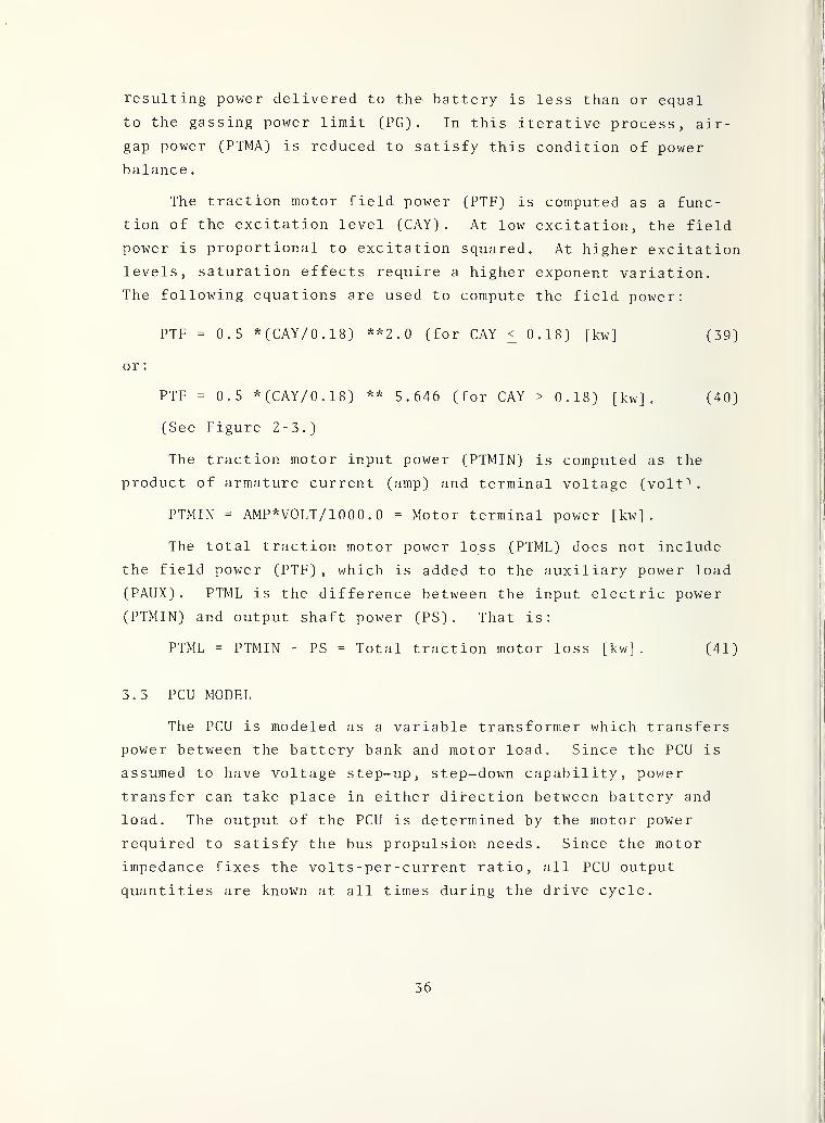
The traction motor field power (PTF) is computed as a func-

tion of the excitation level (CAY). At low excitation, the field

power is proportional to excitation squared. At higher excitation

levels, saturation effects require a higher exponent variation.

The following equations are used to compute the field power:

PTF = 0.5 * (CAY/ 0.18) **2.0 (for CAY < 0.18) [kw] (39)

or

:

PTF = 0.5 * (CAY/ 0.18) ** 5.646 (for CAY > 0.18) [kw] . (40)

(See Figure 2 - 3 .

)

The traction motor input power (PTMIN) is computed as the

product of armature current (amp) and terminal voltage (volt"1

.

PTMIN = AMP*VOLT/ 1 0 0 0 . 0 = Motor terminal power [kw]

.

The total traction motor power loss (PTML) does not include

the field power (PTF), which is added to the auxiliary power load

(PAUX) . PTML is the difference between the input electric power

(PTMIN) and output shaft power (PS). That is:

PTML = PTMIN - PS = Total traction motor loss [kw]. (41)

3.3 PCU MODEL

The PCU is modeled as a variable transformer which transfers

power between the battery bank and motor load. Since the PCU is

assumed to have voltage step-up, step-down capability, power

transfer can take place in either direction between battery and

load. The output of the PCU is determined by the motor power

required to satisfy the bus propulsion needs. Since the motor

impedance fixes the volts -per-current ratio, all PCU output

quantities are known at all times during the drive cycle.

36

The power loss in the PCU is modeled as a three volt drop

times armature current:

Ppcu= -003 x amp [kw] . (42)

The controller input power is equal to the sum of the power

delivered to the motor plus the PCU internal loss.

3.4 BATTERY MODEL

The power demanded from the battery (PB) at each time incre-

ment (TAU) is computed as the sum of the traction motor input

power (PTMIN), the power conditioning unit loss (PCUL)

, and the

total auxiliary power load (PAUX) . The PCU loss is assumed to be

directly proportional to the motor armature current (AMP) . The

auxiliary power term (PAUX) includes the motor field supply power

(PTF) . Additional terms (PAC and PCBLO) can be added to simulate

air conditioning loads.

PB = PTMIN + PCUL + PAUX = Battery Power [kw] (43)

PCUL = 0.003 * ABS (amp) = Power Conditioning unit loss (44)

[kw] .

PAUX = PTF + PTBLO + PBAUX + PECBLO + PLTG + PBC + PAIR (45)

+ PAC + PCBLO = Auxiliary power [kw]

where

:

PTMIN

AMP

PTF

PTBLO = 0.6

PBAUX = 0.2

PECBLO = 0.6

PLTG = 3.6

PBC = 3.2

Traction motor input power [kw]

Traction motor armature current [kw]

Traction motor field power [kw]

Traction motor blower power [kw]

Battery auxiliary power [kw]

Environmental control blower [kw]

Lighting power [kw]

Average battery charger load [kw]

37

PAIR = 1.0 = Average air compressor load [kw]

PAC = 6.0 = Air conditioning compressor power [kw]

PCBLO = 0.6 = Air conditioning condenser blower [kw]

.

The battery is modeled by empirical expressions relating bat-

tery voltage to discharge current (IBAT) and total amp-hours (AH)

discharged by battery. The empirical constants were chosen to

model the water-cooled battery having a 455 amp-hour rating,

based on a shown discharge time. The expressions are strictly

valid for continuous discharge only; for pulsed discharge, the

expressions should be modified to describe the reduced battery

capacity existing in pulsed operation.

The relative state of battery discharge (SB) is given by,

SB = AH/CAP = State of discharge [per-unit] (46)

where :

AH = total ampere-hours removed from battery [AH]

CAP = Instantaneous battery capacity [AH]

The battery capacity (CAP) is given by the empirical relation,

CAP = ABT * (CAYA*ABT**CN-CAYB) = Battery capacity at (47)

current ABT [AH]

where :

ABT = Battery current during discharge [amp ]

CAYA = 937.969 = Current term coefficient

CN = -1.204 = Current term exponent

CAYB = 0.10107 = Constant term [hr ]

The ampere hours discharged (AH) is determined by numerically

integrating the battery current (ABT) over each time interval (TAU)

from the start of the run. Where the value of AH equals 0.6 of the

instantaneous capacity (CAP),the battery is effectively discharged

(SB = 0.6).

38

In the discharge mode,the battery terminal voltage (VBAT)

is described by the following function of battery current (ABT)

and state of discharge (SB)

:

VBAT = ANC * (EO-RB*ABT-CAYD*SB**CM) = Battery terminal (48)

voltage [volt ]

where :

ANC = 256.0 = Number of cells per battery

EO = 2.045 = Open circuit voltage of each cell [volt]

RB = 0.000516 = Internal resistance of each cell [ohm]

ABT = Battery current [amp]

CAYD = 0.419 = Discharge term coefficient

SB = Stage of battery discharge [pu]

CM = 2.24 = Discharge term exponent.

Also :

PB = VBAT * ABT/1000.0 = Battery power [kw] (49)

or

:

VBAT = 1000.0 * PB/ABT = Battery voltage [volt ]. (50)

Equating Equation 48 and Equation 50 yields:

1000.0 * PB/ABT = ANC* (EO-RB*ABT-CAYD*SB**CM) . (51)

Since the state of battery discharge (SB) is a complicated

function of battery current (ABT), the solution of Equation (51)

for battery current is not straightforward. The Newton- Raphson

method is used to determine the battery current (ABT) which satis-

fies Equation (51).

In the charge mode, the battery terminal voltage (VBAT) is

described by the following empirical function of battery current

(ABT) and state of discharge (SB)

:

VCHG = EC + CAYC* (AIC+AIO) * SC ** Q = Charging voltage (52)

per cell [volt ]

39

where

:

EC = 2.0 = Charging constant [volt ].

CAYC = 0.001178 = Charging resistance per cell [ohm ].

AIC = Charging current [amp]

AIO = 42 - 1875 = Offset current [amp]

SC = State of charge [per-unit]

Q = -0.6552 = Charging exponent.

The state of charge (SC) is computed as the total ampere-

hours removed from the battery since the start of the run (AH)

divided by the ampere-hour capacity at the ten-hour discharge rate

(CIO),which is the lowest current discharge for which data was

given . That is

:

SC = AH/C10 = State of Charge [pu] (53)

where :

AH = Total amp-hrs removed from battery [AH]

CIO = 364.219 = Capacity at 10-hour rate [AH]

The battery charging power (PCHG) is given by:

PCHG = ANC * VCHG * AIC/1000.0 = Charging power [kw]. (54)

where :

ANC = 256.0 = Number of cells per battery

VCHG = Charging voltage per cell [volt ]

AIC = Charging current (into the battery is positive AIC)

[amps ]

.

Solving Equation (52) for the charging current (AIC) yields:

AIC = (VCHG - EC) / (CAYC* SC* *Q) - AIO = Charging current (55)

[amp]

.

Substituting Equation (55) into Equation (54),

PCHG = ANC*VCHG* ( (VCHG -EC)/(CAYC*SC**Q)-AI0)/1000.0 (56)

= Charging power [kw] #J

40

The power at which the battery commences gassing (PG) occursat a charging voltage (VCHG) equal to the voltage gassing limit

(EG). The gassing power limit (PG) can be found by setting VCHGequal to EG in Equation 51. That is:

PG = -ANC*EG* ( (EG-EC) / (CAYC*SC**Q) - AI0)/1000.0 (57)= Battery gassing power limit [kw]

.

During charge, the battery power (PB) is kept below the gassinglimit (PG) in magnitude. The negative sign of Equation 57 in-

dicates power flow to the battery. Solving Equation 54 for VCHGand equating it to Equation 52,

1000.0 * PCHG/ (ANC*AIC) = EC + CAY*(AIC + AI0) * SC**Q. (58)

Setting the charging power (PCHG) equal to the battery power (PG)

in Equation 58 and solving for the charging current (AIC) yields,

AIC = (-BC+SQRT(BC**2. 0+4 . 0*AC*CC)/ (2 . 0*AC) (59)= Charging current [amps]

where :

AC = ANC* CAY C * SC ** Q

BC = ANC* (CAYC*SC**Q*AI 0+EC)

CC = 1000.0 * PB.

In the regenerative braking mode, the charging current is

assigned the symbol AIC to distinguish it from the current during

recharge at the end of the mission, which has the symbol ACHG.

During charge, whenever the ampere-hours of the battery (AH) de-

crease, a charging inefficiency is introduced by dividing the

charging ampere-hours by a factor (AHF) which equals 1.1. At the

end of the run, the battery is charged back to its original state

of charge. The charging current (ACHG) is set equal to a maximum

value (AICM) . The charging voltage (VCHG) and power (PCHG) are

then computed from the following equations:

VCHG + EC + CAY C * (AICM + A10) * SC ** Q = Charging (60)

voltage per

cell [volt ]

PCHG = ANC * VCHG * AICM/1000.0 = Charging power [kw] (61)

41

where

:

EC = 2.0 = Charging constant [volt ]

CAYC = 0.001178 = Charging resistance per cell [ohm]

AICM = 70.3125 = Maximum battery current during recharge [amp ]

AI0 = 42.1875 = Offset current [amp ]

SC = State of charge [pu]

Q = -0.6552 = Charging exponent

ANC = 256.0 = Number of cells of battery.

The charging ampere-hours (AH) are computed during each time

increment (TAU),and the state of recharge (SC) is determined as

:

SC = AH/C10 = State of recharge [pu] (62)

where :

AH = Ampere-hours replaced into battery [AH]

CIO = 364.219 = Battery capacity at 10-hour rate [AH]

.

42

4, PROGRAM OPERATION

A flowchart of the computer program is shown in Figure 4-1.

Complete FORTRAN source listings are given in Section 5.1.

Each subroutine is first called to initialize parameters

within that subroutine. On all subsequent calls, the initializa-

tion sections are skipped. Page and column headings are then writ-

ten in the output data file FOR03.DAT and the program enters its

main iteration loop.

At each time increment the subroutine PROF is called first to

determine the mission profile conditions of acceleration, speed,

and position of the vehicle, roadway grade, and encountered head-

wind. PROF also determines the total drag force on the vehicle

and the required accelerating thrust, which is used to compute the

vehicle's acceleration, speed and position at each instant of time.

From the mission profile conditions, the tractive force, propulsion

power, and motor shaft power are calculated. Then the subroutine

MOTOR is called to compute the input electric power to the motor

for the required output shaft power. The battery power is com-

puted as the sum of the motor input power, the power lost in the

PCU and the auxiliary power. The subroutine BATT is then called

to determine battery current, voltage, and state of charge for the

required battery power. The total energy and ampere-hours removed

from the battery since the start of the run are also determined.

If either the battery current limit or gassing power limit is

exceeded, the program reduces the demanded motor shaft power in

small decrements and loops back through the MOTOR subroutine until

the limit is satisfied. The program then writes one line of data

in the output file FOR03.DAT. If plots are desired, one line of

data is also written in the file, FOR22.DAT (this file is required

as input to the plotting program, and contains the value of the

six time-varying system parameters that are to be displayed) . The

time clock is then incremented if the end of the cycle has not

been reached, and the program loops back to PROF for the next

iterat ion

.

43

FIGURE 4-1. PROGRAM FLOWCHART

44

A specified number of driving cycles are made per mile, and

at the end of each cycle, the stop index is incremented, page and

column headings are written in FOR03.DAT, and the next cycle is

begun. At the end of each route, which is a specified number of

miles, the route index is incremented, page and column headings

written, and the next route is begun. At the end of a specified

number of routes, the mission is complete and subroutine BATT is

called to write a run summary, execute the battery recharge model,

and write the recharge results in FOR03.DAT.

The plotting program CHART. FOR can then be executed to dis-

play any six time-varying system parameters on an off-line CALCOMP

pen plotter.

4.1 EXECUTING THE PROGRAM

The main program and all subroutines are contained in separate

source files. By not combining all subroutines into one source

file, compilation time is minimized if changes must be made to only

a few files. The main program and all subroutines must be compiled

and loaded into the computer's active core area before execution

can begin. Loading is done using a command file, BUS.CMD, which

contains the names of all files that must be loaded. Section 5.6

contains a listing of BUS.CMD, and the list of files to be loaded

should correspond exactly to file names and extensions which exist

on the disk area.

Once all files are compiled, the following command is typed

on the user's terminal:

EXECUTE @ BUS.CMD.

The subroutines are then loaded along with the main program

and execution begins. The program first asks the user to specify

one of three typical driving cycles which determine acceleration,

cruising speed, number of stops per mile, route length, etc. A

"1" is typed, followed by a carriage return, if Cycle A is desired,

a "2" for Cycle B, or a "3" for Cycle C. The program then asks

for a code number to indicate which type of output data is desired.

A "1" will cause the output data file, FOR03.DAT, to be generated

(see Section 3.5). A "2" will generate the plot file FOR22.DAT,

which can later be used by the plotting program to produce CALCOMP

plots of system parameters. A "3" will generate both files, a "4"

neither. The code number is typed, followed by a carriage return,

and the program proceeds unassisted. At the end of execution, the

file FOR03.DAT is automatically queued for printing on the line

printer. To print all FORTRAN source files contained in the com-

mand file BUSL.CMD (see Section 3.6) the following command is

given

:

LIST @ BUSL.CMD.

4.2 PLOTTING PROGRAM CHART. FOR

A plotting program has been developed to display any six time-

varying system parameters on an off-line CALCOMP pen plotter.

The program uses the standard CALCOMP subroutine calls, and writes

instructions on a magnetic tape which are later interpreted by the

plotting device to generate the plots. Figures 5-la and 5-lb

(Section 5) show sample plots for Driving Cycles A and B, respec-

tively. The peak values of each parameter must be determined before

execution and the approximate y-axis scales chosen. These scale

values are entered during execution of the program, as are labels

for each of the six strip-charts and the X-axis length in inches.

See References 1 and 2 for further documentation of the plotting

program. Section 5.7 contains a listing of the program which has

the file name CHART. FOR.

46

5 . APPLICATION OF COMPUTER PROGRAM TO BATTERY BUS OPERATION

This section describes the input data required by the Battery

Bus Performance Program and presents typical input data required

to simulate battery bus operation over a prescribed speed-time pro-

file. The input data is listed in Table 5-1 according to the sub-

routine in which it is used; a complete glossary of computer

quantities is given in Appendix A. The results of calculations

based on the input data are displayed in graphical form in Figures

5-la and 5-lb.

Much of the input data required in the program is of general

character and not restricted to a particular type of system com-

ponent. Thus, for example, in the subroutine PROF, data pertaining

to vehicle weight, wind speed, and acceleration are required in any

program in which a vehicle is being modeled. In other cases, how-

ever, the input data is related to the specific type of system com-

ponent being used. In this program, the subroutine MOTOR models a

shunt wound dc motor with power loss in the field winding in addi-

tion to the other loss contributions. The use of other dc motor

types would require different program statements and corresponding

set of input data to be used. The list of input data presented in

Table 5-1 is meant to show the general requirements of this program

and familiarize the reader with the type of data used in the

program

.

47

40.00

VEH 1 CLESPEED( MPH )

0.00

7 500.00

TRACT 1 VEFORCE1 LBS )

-T500. 00

400.00

PROPULS 1 ONPOWER( KW )

-400.00

0.00 25 .00 42.00 63.00 04.00 105.00 1 20.00

FIGURE 5-la. CALCOMP PLOTS OF SYSTEM PARAMETERS - DRIVING CYCLE A

48

400.00

PROPULS 1 ONPOWERf KW )

-400.00

200.^30

MOTORPOWER( KW )

-200.00

500.00

BATTERYCURRENT( AMPS )

-500.00

200.00

BATTERYPOWER( KW )

-200.00

zT

0.00 23.00 46.00 69.00 92 . 00 5.00 38.00

FIGURE 5- lb. CALCOMP PLOTS OF SYSTEM PARAMETERS - DRIVING CYCLE B

49

TABLE 5-1. COMPUTER INPUT DATA

Input Data Required by MAIN

TAU Computing interval 1.0 sec

TIMX Output interval 1 . 0 sec

ETAG Rear end efficiency . 945

PAC Air conditioning compressor power 6.0 kw

PCBLO Air conditioning compressor blower 0.6 kw

PECBLO Environmental control blower 0.6 kw

PAIR Average air compressor load 1.0 kw

PLTG Lighting power 3.6 kw

PBC Average battery charger load 3.2 kw

PTBLO Traction motor blower power 0.6 kw

PBAUX Battery auxiliary power 0.2 kw

I AC Air conditioning control mode 0

Input Data Required by Subroutine PROF

AJERK Jerk rate2

3 . 5 mph/sec

PHIW Wind direction 0.0 deg

PHIR Route direction 0.0 deg

WS Wind speed 0 . 0 mph

AF Vehicle frontal area 80. ft2

CR Coefficient of rolling friction .005 lbf/lbm

WTCRB Curb weight of vehicle 36,400 lb

WTP Weight of typical passenger 150 lb

Data for drive Cycle B:

ACCM Maximum acceleration 3.5 mph/sec

DECL Deceleration 3 . 5 mph/ sec

VC Cruise speed 31 mph

NS Number of stops per mile 8

DWELL Dwell time at stop 16 sec

TAUMU Makeup time 0 sec

NP Number of passengers 20

SR Route length 2 miles

NT Number of routes per mission 1

50

TABLE 5-1. COMPUTER INPUT DATA (CONTINUED)

Input Data Required by Subroutine MOTOR

AMPMO

AMPMG

VOLTMA

VOLTMD

VB

RTMA

RATIO

TF

CAYOA

CAYOD

CAYOG

PSMA

PSMD

Maximum traction motor current-

normal

Maximum traction motor current-

on grade

Maximum traction motor input

voltage - accel

.

Maximum traction motor input

voltage-decel

.

Brush drop

Traction motor armature

resistance

Reduction gear ratio

Tire factor

Excitation 1 imit - accelerat ion

Excitation limit-deceleration

Excitation limit on grade

Maximum shaft power-acceleration

Maximum shaft power-deceleration

Input Data Required by Subroutine BATT

700. amp

770. amp

530. amp

600. amp

2.0 volt

.0405 ohm

11.42

8.003

.215

. 23

. 25

223.7 kw

223.7 kw

ANC

ABM

EO

EC

EG

AHR

SBO

CIO

DD

CN

Number of cells in battery

Max. allowable battery discharge

current

Open circuit battery voltage

Battery charging equation constant

Battery gassing voltage

Rated battery capacity

Initial state of discharge

Battery capacity at 10 hour rate

Depth of discharge

Exponent in battery capacity

equation

256.

421.88 amp

2.045 volts

2 .

2.6 volts

3.19.9 amp -

h

.05

364.2 amp -

h

0.6

-1.204

51

TABLE 5-1. COMPUTER INPUT DATA (CONTINUED) !

Input Data Required by Subroutine BATT (Continued)

CM

CAYA

CAYB

CAYC

CAYD

AIO

Q

RB

AI CM

ETACHG

AHF

Exponent in discharge equation

Coefficient in battery capacity

equation

Constant in battery capacity

equat ion

Factor in charging equation

Coefficient in discharge equation

Offset current in charging voltage

equation

Exponent in charging equation

Battery resistance in discharge

equation

Maximum charging current

Wayside charging station efficienc

Ampere-hour factor

2 . 24

939.07

.10107

.001178

.419

4 2. 188 amp

- .6552

.00516 ohm

70.35 amp

y .96

1.1

52

5.1 FORTRAN SOURCE LISTINGS AND DATA FILES

53

MAIN. FOR

C »»»» BATTER! BUS PEPFOR_M_ANCE PROGRAM 1

COMMON /C P R 0 F / w Tc R B , T A U 1 , I A C , I D C , VC , N s /sS ,0 W E LL , T A U M U , N p”, W T , SR>NT,I SN»TStT4 »TA U t JM, isw, AJE RKR, AF ^DtC Ri ACCM t PECLCOMMON /CMOTOR/INO, AMPMo#AMPMG, VOLTMA,VOLTMD, VB,RTMa/rATIO,

'

» TF,CAYQA ,CAYOD»CATQG,PSMA f PSMp _____COMMON /CPCU/PAC, PCBLO | pECBLO , PA IR , PLTG, PBC , PTRLO , PBAUXCOMMON /CBATT/EBA T, S , THET a, X 1 , ANC j_ABM , , EC , FG , AHR , SB0 , C 1 0

,

# DU,CN#CM,CAYA,CAYB,CAYC,CAYD, AIo#G»R 8# AICM,ETACHG, AHF,TEMpDATA TAP 1/1.0 /»T lMx/l ,p/ f E T AG/p.945 / tA AC/O/ __

C#**# SPECIFY DRIVING CYCLE?WHITE (5« 214 )

READ (5 » 215) I DCC+*»» SPECIFY OUTPUT FILES? __

WRITE (5,

2

18 )

READ ( 5 > 2 1 5

)

IQFIK(IOF t EQ e l),OK,(IOF,EQ,3)) 11*1IFC(IUF.EQ.2),OH.(10F,EQ.3)) 12*1 _WRITE(5,216)

c »»*« initiali zati on?1*011*1JM»iCALL pRQF(VfACC, GRADE, Hw, S,TN,TD) _ __C A L L B AT T t V BA T , A B T , P B , P G , A H , T A U , I N D )

IF(I |.N fc;.t ) GO T O 35 ^ __C#### OUTPUT PAGE HEADING?

WRITE(3,2l7) WTCRB, I F, RATIO, A f ,CR,CDIF(IDC.EG.l) WRIT£C3,211)IFCIPC.EQ.2) WR ITE ( 3 , 2

1

2

)

IFCIDC.EQ.3) WRITEC3,213)WRITE ( 3 , 22 1 ) SR # NI # N$*AMPMq# AMPMG , VOLTMA , VOLTMD,

# rtma,psma,psmd,eo,anc,eg,ahr,rb,abm “

c*##« INITIALIZE cycle data?is isw*

t

ACC»0 a 0 1

V»o®0|TAUbTAU I/5.0 __tim®o 9 0

HC*1SNaSTSSIFCIl.NE.i) GO TO 40

C##«# OUTPUT CYCLE DATA?WRITEC3# 2©3) I,II,SS,NP,WT,VC,ACCM,DECL,DW£LL,HW

c*»«» Output driving cycle?IFgIDc,EQ,|) WRITE C3 »21I)fFTTDcTEQ.21 WRITE ( 3 , 2 1 2

)

IFCIDC.EQ. 3) WRITE ( 3 ,213 ) ;

C*### OUTPUT AIR CONDITIONING STATUS’?IF(IAC.EQ.t) W RI TE(3,2 0&)IFCIAC.EQ.O) WRITEC 3, 202)

€»»*« OUTPUT COLUMN HEADINGS!;

WRITEgl, 204)

54

MAIN. FOR (CON'T.)

C»#»# DETE RMI NE PROFILE CONDITIONS |

40 CALL pROF(V, ACC, GRADE, HW,S,TN,TD)IF(T S t GT.T4) GO TO 60 l END OF C YCLE 1

C##*# COMPUTE TRACTIVE FORCE, PROPULSION POWER, AND MOTOR SHAFT POWER*TP«TN»TPPw«o,o01989*TP*VIFCTP. LT. 0.0? PS»PW»ETAGIF(TP.GE.O.O) PS»PW/ETAGPSfP S _

C##*# COMPUTE TRACTION MOTOR CURRENT, VOLTAGE, I NPUT POWER, AND LOSSES*45 CALL MOTOR(PS,V, GRADE, AMP, VOLT, VBAT, CAY, PTF)

P T M I N

V

Q L TfA Mp/IQQQ.QPTMLbABSCPTMIN.PS)

C*##t COMPUTE PCU LOSSES A HP AUXILIARY POWER i

CALL PCU CAMP, VOLT, ABT, VBAT,PCUL,PAUX,PTF, IAC)C*### C OMPUTE BATTERY POWER. CURRENT* VOLTAGE, AND AMpERE-HgURS I

PU»PTMlNtPCUL+PAUXOALL_MIUV_B ATjlMIaP_B,_P£, AitilAU,IM1IFCIND.EQ.l) GO TO 45 JPOWER LIMITED MODE

|

IFCJND.EQ.2I GO TO 70 ... IBATTERY DISCHARGED!IFCPTMIN.GE.O.O) PGaO.O

C_*_*_t# UPDATEL TRACTIVE FORCE AND PROPULSION ANP_ BRAKING POWERLIFCTP.CT.O.O) TNiTN- CCPS1»PS)#ETAG)/ CO. 001989# CV40. 001)

)

TPaTN+T D I _____IFCTP.GE.O.O) PWbPS#ETAGIF(TP*LT.Q.O) pf»pw-ps/etagIFCTP.CT.O.O) PF«0 ,

0

C#»»# OUTPUT TIME HISTORY OVER CYCLE* _ _____I F c c I WC , EQ, 1 ) , AND , cU . EQ , 1 ) ) WRITE C 3 , 206 ) THETA , ACC , V , S , GRADE , TP

,

f TNj AMp, VOLT, ABT, VB AT, AH, PG, PB t PAUX,PCUL, PTML,PTMIN,pS, PW,pFIFCClWC,EQ,n,AND.Cl 2 .EQ,l)) WRITE C 22 , 21 9 ) THETA, V, TP, PW,PTMIN,

|_ ABT^PB ___IFCV.GT.VP) VP»VIFCA8$CTP),GT 4 ABSJTPP)) TPPaTPIFCABSCPW) .GT.ABSCPWP) ) PWpaPWIF CABS CPTMIN).GT.ABSCPTMINP) ) PTM INpapTMINIF CABS (ABT) , GT.ABSC ABTP) ) ABTP«ABTIF (ABs(PB) # GT ,AB5(PBP ) ) PBPfPBIWC«0

C*### INCREMENT PRINT CLOCK*TlMiflMVrAUIFCTIM^GE^TIMX) IWC«1IFCTIM.GE.TIMX) TIMio.O

C*###_INCREMENT run time clock*THE fAs T HETA TAUIFCTHeTA.GT. 10000,0) STOPGO TO 40

C»»#» END OF CYCLE* __60 TS«0.0

iPlfiii»i+iIF(S,GE,vJM«SR«0,05) go to 65

55

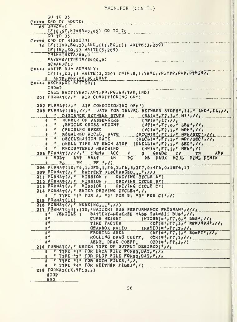
MAIN. FOR (CON'T.)

C*##«65

C*«»«7 0 WRITE (3/209

5

GU TO 35END OF ROUTE* -----

IF(S,GT fNT#SR®0*05) GO TO 70

GO TO 35END OF MISSION*IF ( ( IND # EQ , 2 5 , AND # ( i 1,EQ # l )

)

_IFi^INd,EG^2) W R I T E ( 5 » 2 0 9 ) _T^IN axHETA / 60 « 0VAVE«S/(THETA/3600,0)SC® AH/C 1

0

C#**« WRITE RUN SUMMARY*IF(It,EQ # l) WRITE(3,220} TMIN

, S , I , VAVE , VP , TPP, PWP, PTMINp

,

« ABTp^PBP, AHjJCjJBATc##t« recharge battery*

IND®2 _ _CALL BATT(VBAT,ART,PB,PG, AH,TAU,IND)

201 FORMAT ( / ,* air conditioning ON*)

202 FORMATC/,*203

204

AIRFORMATdHi,//, • DATA

J^I STANCE JET WEENNUMBER OF PASSENGERSVEHICLE GROSS, WEIGHTCRUISING SPEED

CONDITIONING OFF/

)

FOR TRAVEL BETWEENSTOPS (SS)®*,F7.3, *

STOPS*, 14,

*

AND*, 14,//,M g f//i__

REQUIRED ACCEL* RATEdeceleration RATEjwell time at each stop

(NP)®',I7,//CWT)«*jF 7 , 0 i

(VC)»*,F7.l#(ACCM)®' # F 7 ,i #

(DECL)®^,F7,I,IPAELLlfAiZlxijL

(HW)a*,F7.1,S GRAD E

w,n,

MPH* , /)TP TN

206.209

ENCOUNTERED headwindFORMAT! ////j * THETA ACC V

VOLT AST VBAT AH PGPS _ pw PF *,/)

FORMAT ( IX,

F

6 1 1 , 2F5 • 1 ,F 6 1 2 , Fb

«

3 ^ 2 F 7 • 0 , 4F 6 « 0 , 10F6 a 1 )

MPH *,//,MPH/gBC*, //,MPH/gEC*,//,SEC*,//,

AMPPB PAUX PCUL PTML PTMIN

F£«MAI1/Ii BATTERYMISSIONMISSIONMISSION

211 FORMAT*/,*.112 FORMAT*/,

•

213 FORMAT in 9

214 FORMAT (/f * ENTER• • TYPE M* FOR

215 FORMAT C X 1

}

jJJ±disc harged. ..

i DRIVING cycle A*)I driving cycle B*)8 DRIVING CYCLE C*3

DRIVING CYCLE**,/,A, FOR if FOR Cl *,/)

216 FORMAT*/,* WORKING# ##*,//)217 F0RMATClH | y i3X,*BATTERY BUS PERFORMANCE PROGRAM* , ///,

* vehicle I battery-powered mass transTt BUS* | //#* CURS WEIGHT (WTCR1)®%F7#0, * LBS*,//,* TIRE FACTOR fWWFTrTTiTT bPm/mph#

GEARBOX RATIOfrowal areaROL LINGD RAGCOEFF,

(TF)»*,F7*

*

RPM/MPH *,//,(RATIO)®*, F7#2,//i

(AF j»*,F7*i* 0 SQ«rT*,// #

(CR)«t*,F7.|,//,

218AERO, DRAG COEFF, CCD)® * , F7#3, /)

FORMITC/,* ENTER TYPE OF OUTPUT DESI RED* *,/,'T Type “i "FOR DATATTLE FOrojTDAT, *,/,* TYPE "2® for PLOT FILE FOR22,DAT,* t /»

"^TYff *1* FOR BOTH FILES,*,//• TYPE *4" for NEITHER FILE**,/)

2 i ITOrMatC jX, 7 FTo • 3 j

STOPEND

56

PROF. FOR

SUBROUTINE PROF (V, ACC >GRADEyHw ,SfTN,TP)DIMENSION G ( 25 # 2 )

COMMON /CPROF/WTCRBf TAUI » IAC» IDCt VC»N8»SSt DWELLj TAUMU»NR# WT<SR» NT»I SN,tS # T4#TAU,JM, I5W, AJERKR,AF,CD#CR#ACCM,DEClDATA CEE/21 ,927/« AJERKR/3.5/ t PHIR/0.0/#PHIW/Q.0/,W8/0.0/,

« AF/86 t 0/#CD/0«84/»CR/0.005/fWTCRB/S6400 t 0/»WTP/lS0«0/CQ TO 1000 _ _

XNI»lC»»»• INI TIALIZAT I ON!

IFCIDC.EO.l) GO TO 1

_ ir(IDC.EQ.2) GO TO 2XF(IDC,EQ,3) GO TO 3

C»»»« DRIVING CYCLE A |

1 ACCM»i # 44

2x2_VCwJl.ONS«4 _____SS«I a 0/N8DwELL»3Q,0 _taumu»o.oNP«133Rl6 •

0

NT«4^

GO TO 4

C*tH DRIVING CYCLE B|

2 ACCM«3 ,5DECL«3 a 5VC *3 1.0N5«8SSP1.0/NSDWELL»16 # 0fSUMU.0,0NPP20SR«6,0NTMGO TO 4

C***# DRIVING CYCLE Cl3 ACCM-2.5

DECL«2t 5VC«25,0NS>58S«i, 0 /NSDWELL.20.4TAUMU.330,0NP«0SR»6,0NT»4

57

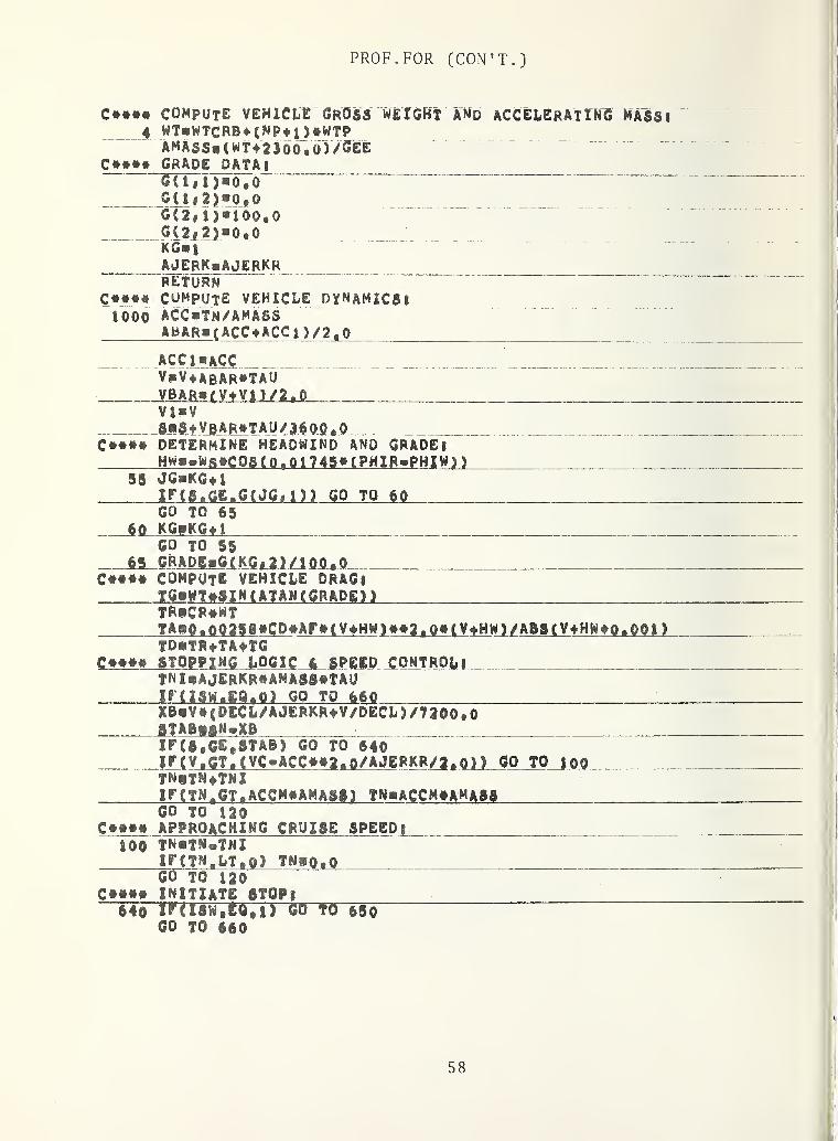
PROF. FOR (CON'T.)

C###« compute vehicle Gross weight and accelerating massi4 WT«WTCRB4(NP*j 5*WTPAMASS* ( WTt2 300 ", 6 ) /GEE

C#### GRADE DATA!T!TT7i)«o7o

" "

CU f 2 )«0,0G(27i)»100,0G(2 f 22»©,0KG* i

AJERKsAJERKRRETURN

€*»## COMPUTE VEHICLE DYNAMICS S

iooo acc»tn/amassABAR»(ACC»ACCl)/2.0

ACC 1 *ACC _VpV*ABAR*TAU

V1*VSlS*VBAR»TAU/36Q0 # 0DETERMINE HEADWIND AND GRADE!HW«j»Ws»CPSCQ,0i745» ( PHlR«PHIW)) __

55 JGPKGfiIUSlbJB&mS C JQ gJJl_GP_...T.Q_iQGO TO 65

60 KGflKGf l

GO TO 5565 GftADB»GCKG»2)/100 f 0

C#### COMPUTE VEHICLE DRAG!TG*WT»8 IN (ATAN (GRADE)

)

tr*cr#wtTA»0.002S8»CD»AF»(V» H W

)

»»2.0»(V»HW )/ABS(V*HW»0.001)TDpTR^TA^TG

C»»»» STOPPING LOGIC & SPEED CONTROjy

_

TNI*AJERKR#AMASS«TAUHUM »,I 9XB*V#(DECL/AJERKR*V/DECL)/7300.0STA 8MN.XB

:

IE(S®GE®STAS) GO TO 64©___ IF( VaGT» ( VC«ACC*R 2 a 0/AJERKR/2 t 0) ) GO TO 10Q_

TNBTfHTNIirgTN t GT»ACSM»AMASS) TN *ACCM»AMAi§GO TO 120

c»tt» APPROACH I NG cruis e SPEED I __

10© TN»TN®TNII F c

T

N.LTaO) TNip.oGO TO 120

c*##« INITIATE stop*“T4©"ircMw»e®al' ww ©so

'

GO TO ©60

58

PROF. FOR (CON'T.)

650 ACC»0,0TlwDECWAJERKRT2RV/DECLT3»Tl»T2T4pT3*DWELLIF(S.GE.JM»gR»Q,l) T41T44TAUMUISWaoTSao.o

660 TSvTS+TAUIF(TS.CT.Tl) GO TO 670

C#tM ONSET |

AJERKa-AJERKRGO TO 692

_ 670 IF(TS.GT.T2) GOTO &8QC*»«« DECELERATION!

AJERKwQ.Oacc«-declGO TO 694

680 IFCTS,GT,T3) GO TO 690C»t»» FLAIRi

AJERK.AJERKRGO TO 692

690 IF(TS.GT,T4) GO TO 120C»»»» DWELL

|

AJERKbO,

0

ACCJO . 0

VlO.OQlTN*0,0TD»Q.O8*8NTAUaTAUlGO TO 120

694L20

tn«acc*amassRETURNEND

59

MOTOR. FOR

SUBROUTINE motor (PS »V» ORADE,A MP,VQLT»VBAT,CAY,PtF )

vunruyKJL TF,C»YOA»CSYQPtC»yO<l>P8H.A,P...„

TA AMpMo/700,0/»AMPMC/770 # 0/#VOlTMA/5lO # 0/#VOLTMD/600 # 0/fVB /JUft/j RTMA/0^4 0 4 9 / «RATIO/li.42/«Tr/»Apo3/,CA¥oA/'O,215/#CA¥00/Oe23/»CA¥0G^8 # 23/#P®NA/22S.7/fP8MD/223,7/irn orr motor ir vehicle is at rssufV.LE.ft.Oll CAYpft.ftftftl

DATA

C»»«» TURN orr MOTORIFCV.Ll. 0,013 CAYPOeOOOiIFCV.LE. 0*013 AMPpQaQirev.LE. 0.013 VOLT«VSATIF(V.LE.Q. Ol) PTFpp.O _____IFCV.LE, 0,013 RETURN

CtffJL

R

EDUCE SHAfT POWER IF IN POWER LIMITED MQDElIF(INd,EQ«13 PSpP8*0,95JF-UlNJDj.E^.^JL) gO_?Q__lAD

C*«*« COMPUTE motor speed

|

RPMpRATIQ»TF»VIF (PS.GE.O.O) GO TO 135

C»»»» BRAKING MOD E PO WER, VOLTAGE, an d EXCITATION LIMITS!IF (ABs(PS) , GT jPSMD J P8P-PSMDVODTMaVOLTMDCA¥OpCA¥OD

_ GO TO 1 45C***« MOTORING mode POWER, VOLTAGE, AND EXCITATION LIMITS

f

135 IF(ABsCPS)*GT f PSM A3 PSpPSMA]

VOLTMaVOLTMAIFCV0LTM a GE a VBAT3 VOLTMaVBATCAYpiCAYOA

c»»»» ARMATURE CURRENT LIMIT AND INCREASES LIMITS ON GRADEl143 AMPMpAMPMo

IFCGRADE.GT.O.S53 AMPMpAMPMGIF (GRADE, GT ,p # 15 3 CAYqpCAYqG

60

PROF. FOR (CON'T.)

C*»»» TRACTION MOTOR LOSSES! _ptmb»o«ooi*rpmPTMW« 1 , 475»(RPM/454 q > q)»»2i0

16o PTMIb2,629E»o4*CAX##i

,

29#RPM##i ,4o6C###* compute AIR CAP POWER

|

PTMA« ( PS4PTMB4PTMW4PTMI ) To , 99c#### determine excitation constant cay t

Cl«(VOLTM-VB)/RPM"C2«4Qo0 .0»PTMA»RTMA/(RPM»»2.0)CAYV«(Cl4SQRTCCj##2.0-C2)j/2,0CAYI«1000.0*PTMA/(RPM#AMPM)IF(CAYV # GT,CAYI) go TO 17o

__16 ? PS«Q .99»PS-GO TO 160

1 7<L IF(CAYO.GT.CAYV) GO TO 175CAYjpC ayoIfJCAYxGTjCAYIJ_Gg TO 180 _GO fO 165

175 CAYwCAYV .C##*# UPDATE IRON LOSS AND AlR GAP pOwER IF CAY RESET

|

180 PTMI f2.629E«04»CAY»»l a 29»RPM»»i.4QSPTMAvpTMAfPTMI 1«PTMICW COMPUTE ARMATURE CURRENT, TERMINAL VOLTAGE, AND FIELD PQWERlAMPii 000.0*PTMA/(CAY#RPM)V0LT»CAY»RPM»VB4AMP»RTMAlF(CAY,LE,o« 18 ) PTF*o.5*(CAY/0.l8)#*2.0IF (CAY.GT.O . 18 ) PTFi>0.5»(CAY/0 .18) »»5 .646RETURNEND

BATT . FOR (CON’T)

SUBROUTINE b A t

t

c V B A T ,

A

b t

,

pB #

P

g # a

h

# t A U , I N D

)

COMMON /C BA T T / EB A T , 5 # T HETA # 1 1 * A n C # A B M , E0 # EC # EG # A H R # 8B 0 # C 1 0 #

L__DDiC*U£»UiyLYAxCAVB,CA YCj C AYPj AlO * Q#RB * A_I£M , ETACHGfAHFjTE M pDATA ANC/256,0/#ABM/421 t875/#Eo/2,045/#EC/2.0/#EG/2,6/»

f AHR/3l9.922/gSBo/Q,o5/»ClO/364 f 21 9/» DD/0^6/ y CN/«l t 2Q4/y# CM/ 2 .24/#CAYA/937,969/,CAYB/0 B 10107/ #CAYC/0,001 178/#

_ » CAYp/o,4l90/>AlQ/42.1873/ # Q/»o.6552/>RB/Q.ooo5l6/» _« AICM/70,3125/#ETACHG/0,96/#AHF/1,1/#TEMP/|o,0/#TEMPM/30,0/#I TEMpr/100. 0/ _irCINl.EO.l) GO TO 1©0@LNJPl

c##*# INITIALIZATION!AH©CiQ#§BOvbat«ieo*ancJETUM '

1000 IF(INd,EQ.2) GO TO 720 {EXECUTE RECHARGE MODEL I

INDfO ^NORMAL OPERATION]C*##« COMPUTE APPROXIMATE VALUE OF BATTERY CURRENT!

_ABt»!&00jO#Jb /(Eo*anc3IF (AST .01,0,0) GO TO 700

c*### BATTERjf CHARGINO|_ۥ*# COMPUTE state of CHARGES

SCdAH/ClO _ _____C««*« COMPUTE GASSING POWER LIMITS

PG*®AnC#EG#C (EC«EC)/ (CAYC»0C«*Q) »AIo)/1 000.0UCPB.LT.PC) IND»1 {GASSING POWER LIMIT EXCEEDED 1

IFCINDbEO.I) RETURN€«##• COMPUTETHARGlNfi CURRENTS

AC«ANC#CAYC«$C**QBC»AC»AiotANC#ECCCwiOoO-ORPi

“AICi(.BC«SQRT (BC*#2 * 0®4,0»AC#CC J 3/(2.0»AC}ABTs®aIC

Ct«*« COHpU'fE "battery voltagesVBAT^ iOOO.O^J® # CX8Tto«OC1

)

GO TO 711c®##« iATTERY discharging^ _ _

70© IF (ABf, £0,0,0 ) AB T •0,001£#### COMPUTE BATTERY CAPACITY!

CXPa(CAYA*ABT4H»CN®CAYB)«ABT€##»« CORRECT CAPACITY FOR TEMPERATURE VARIATION

g

FACT»i t 04(TEMp.TEMPM) /TEMP

F

cap«cap*factC**## COMPUTE state or DISCHARGE 8

_

SBhAH/CAPC##*# COMPUTE CURRENT CORRECTION FACTORS!

ZETArE0®RB#ABT®CAYD#8Br#CMM 000.0#PB/(ABT#ANC)EETAPp«RB^CAYD#fM#CAYA#SB*oCM#AiT«H»(CN»l ,©)

# 41000. 0«PB/(ANC#ABT##2.0J'

mr«ZCTA/ZETAP- '

IFCAiSCDELD.LTjJ,©) GO TO 710 1 ITERATION COMPLETE!

62

BATT.FOR (CON'T.)

€•••• correct battery CURRENT

I

ABfABT-PELIIF( ABt«GT # ABM) INDm iBATTERY CURRENT LIMIT EXCEEDED!IF (INPaEOa 1 ) RETURN

C««H iterate to refine BATTERY CURRENT APPROXIMATIONSGO TO 700

c«««« COMPUTE BATTERY VOLTAGE

|

710 VBAT»ANC»(EQ>RB»ABT*CAYD»aB»»CM)C*### COMPUTE AVERAGE BATTERY POWER, ENERGY# AND AMPERE-HOURS!

711 PBAVEi(PB+PB1)/2.0

pgl fPB i

EBAT«EBAT+PBAVE*TAU/3600,0ABTAVEftABT»ABTn/2^QabthabtDELAH»ABTAVE«TAU/ 3600 f 0IF(DELAH,LT,O t O) DELAHpDELAH/AHFAH fAH»PELAH ,

IF(AH,GT,DD#AHR) IND«2 IBATTERY DISCHARGED

J

REIMiLcm** BATTERY RECHARGE MODEL!

7 20 TAU ieo.O __C*«*« OUTPUT CHARGING DATA COLUMN HEADINGS!

ircn.BQ.l) WRlTEQf 810 )

c***« COMPUTE STATE OF RECHARGE!710 _S£fAH/CUE

lF(5C,LE t SB0) GO TO 760 J RECHARGE COMPLETE!C#»»» COMp UtE REC HARGE CURREN T AND VOLTAGE!

ACHG« (EG-EC ) / (CAYC«5C#»Q j -AIOIF(ACHG.GT.AICM) GO TO 740VCHGpeGGO TO 750

740 ACHGVAICMVC HG«EC+CAYC »( ACHG*AIo)»SC»»Q

C*«»« COMPUTE RECHARGE POWER, ENERGY, AND AMPERE-HOURS I

750 PCHG»ANC»VCHG»ACHG/10Q0.0ECHG*PCHG«TAU/3600.0+ECHGAH»AH-ACHG»TAU/(36 00.Q»AHF)CHGTlM»CHGTIM^TAU/60 # 0

C*M* OUTPUT RECHARGING DATA!I F ( 1 1 , EQ , i ) WR I TE( 3 , 8 20) CHGTIM , SC,ACHG , VC HG , PCHG , AH, ECHGGO TO 730 1C0NTINUE ITERATION!

63o

BATT . FOR (CON’T.)

RECHARGE COMPLETE!1§© 8Csfi.Se

COMPUTE’ SPfCiriC CHARGING IMErGiesiEPMsECHG/8EPMjwePM/ETACHG

C»»»» COMPUTE OVERFALL BATTERY EFFICIENCY !

EFFiAf«E@AT/EC HGc*t*« OUTPUT RESULTS OF BATTERY RECHARGE

|

irai,EQ # i) WRtTC(J f S30) CHGttM # SC#EPM,EPMi,EFflATil d FPRHATUHi,///,* BATTERY CW&GRlMG PATA8 # #// <

« * CHGTIM sc achg vcho pchg ah echg»,/>820 FQRMAT(lXgF6 t l y F7 t 3fF6 t l»rSii2g3r6 t U830 FORMAT(//» # RESULTS OF BATTERY RECHARGE) % //,

|» CHARGING TIME CCHGTIM|j* 9 Ffe,lf f MIN*,//,f» STATE OF CHARGE (8C)«*tF6,)t* PU*,//#9» SPECIFIC ENERGY AT BATTER l_l NpUT (EPM)>*,FS %» 9 KWHR/MI * t // 1

#• SPECIFIC ENERGY AT CHG, 8TA, INPUT (EPM! $|»',F6,2, * KWHR/MI #j> //#

9* BATTERY EFF ICIENCY (EFPBAT) »**F6,3« * PV §UlSTOPEND

64

5.2 BATTERY BUS PERFORMANCE PROGRAM

65

BATTERY

BUS

PERFORMANCE

PROGRAM

M•J

e-

cumH

04

m&>oCO

w09

&«M

Wu

HCO

a

030*m

M

04!

I

MCOCO

OM03o<co

COwD03CJ

<*3

S3B*£2)

3M©(B3

909

M09

am0309

BOUmM

Si

&

cqeq

&a

s

8

030*

a

3j

i

g

oJH

i

66

BATTERY

BUS

PERFORMANCE

PROGRAM

a a oo m « 0 Cl 9 0 1A Pi m m 0 9 o ooo• « • • • i • • • « & • • + © © • © G ©

oo o o <»> 9 • e* 9 (*•9 9 pr o M 9 o e> ooCD sC m m or* a m « •

•- •- l i T i 4

9 9 OP Pi AAAA Pi 9« A 9> • P-9 oo« « 9 O 04 9

iS0 0 S31 1

•f 9 p • o o«M Pi 04 S

» ss90 IT Pi *“1 t

<n pi CM CM AA A AA Ao m 0> Pi iN » oo9 9CM CM

cr KCM r 0 m0 0 oo0 0 33 M 009 0 A O

Pi 1

bbi i i 4 1 i i 1 i • • 1 • 1

cn cn 9 IH• 9 « 09 9 9 9 A to co r- oo• 4 • t • • « * • o • • • e • • • • •

o o o *- rn 0 P4 <"> 0 0 pi i*» 0 m m m 0 9 oo0 cn m 0 0 0 0 0 0 0 0 0 0 0 n p* Pi 1• 1 1 1 1 » » i i 1 1 1

1

1

c*« CM 4T- M p* CM CM 0 0 0 0 9 A9 9 o oooo a OOo ooo o oo o o o o o 0 0 oo1- 0 r* 0 r* cm0 CM Pi Pi 0 0 0 0 Pi Pi Pi Pi 0 0• 4 • • • • • • • « • • • • • • • • • •

9 9 o o O t- 0 0 0 0 0 0 0 0 0 0 9 9

to IO 9 v tn o ooo ooooooo o oooO O O 0 •- <s CM CM 0 0 0 0 0 0 Pi PI CM 0 o o

m cn 0 0 r- 9 * 9 ^ r* 9 0 P» r~ 00 0 9 9 PIP*• 4 • • • »

*i• 4 • • • • © • • • • •

o o s? P4 »- 0 0 0 0 0 0 Pi Pi Pi Pi 9 9 9 99 9 0 0 Pi Pi Pi Pi Pi Pi 0 0 i

1 1 i i 1 1 i i 1 1 1 1

o o o o O 9oo 9 9 9 9 9 9 9 CO CD 00 ooo o © m 0 0 0 0 Pi Pi Pi Pi Pi Pi Pi Pi CM 0 oo

CM P« Pi 0 0 0 0 Pi Pi Pi Pi 0 0 0 0

9 9 9 9 9 ® o art 9 9 9 00 CO 9 GO GO GO GO 00 00• « • • • • . • • i • • • • • • • • • •

<7» 9 9 9 9 9 9 9 9 9 9 9 9 9 9 9 9 9 9 9

• 4 • • • • • • • • • • • • • • • • • •cn CT 0 o 9 0 0 9 0 0 0 «r 9 9 9 9 r- 0 p» pir f o 9 9 9 9 sO 9 9 9 9 9 A A 0 0 0 09 m 9 vO 9 9 9 9 9 9 9 9 9 9 9 9 9 9 9 9

•

GO GC GO CM • »n pIW 0 0 0 9 9 9 9 9 9 0 CD oot" r* r- i m pi 0 0 0 0 0 0 0 0 0 0 0 0

I 1 i > i i t I • 1 ' * i

m rrgo oo

0 co9 O £8 ss£8S333 33 33 9 90 0

*- *4 0 CM Pi Pt pi ri 0 0 pf p*00 pi Pi 0 0 0 0• 1 • • • % • » • « • • • • • • • © • •

o o o O O O o oO O o o oo oo o o oo. « • • • • • • • • • • • • • « • • • •

o ooo o 0 r* o © 0 9 9 O O 0 so Pi Pi0 rr p> o e « 0 9 « 9 9 9 90 3S SO 09 9 9 M> SO 99 • 00 0 00

• • • • • • • • « • • • • © • « • • •

r- r» r- 9 9 0 9 4* 0 9 Pi 0 9 * 0 CD 9 9 99 m 9 0 tn tn 9 9 h CO 9 0 0 9 0 0 9 9• • i 1 1 1 1 9 0 0 0 0 0 0 0

i i i i i • i

0 0 o ve 4 4T 9 car t* 9 9 9 9 9 9 009 CM CMICM CN 0 0 0 0 pi pi 0 0 0 0NO tr r* 0 0 0 0 0 0 0 0 0 0 0 0i * * * 9 * * «r * 9 9 9 9 9 9

1 1 1 1 t • i • 9 « • i 1 1

•

O so 0 T- 0 0 0 9 9 GO 9 O OsO sC \C 9harm 9 9 GO 9 O 00 0 0 0m 0 m cm r* p*:€0 G© 9 9 GO GO 9 PiP Wt 9 9

• 0 0|003 ! ! ?

0 0S 1

0 01 I

0 0|0 0! ! ! !

0 03 !

o o o o o oo o o o o oo o O O S o O O o oo c o o o c o oo o o a o o o oo o o o o oo o ooo o o oo o o o o o• • • • • • • • • • • • ® • • • • • •

o o o o 0 9 0 0 o oo o O OIO o o o o or- r- 9 9 OOI'N 0 0 =* J7 9 AA A 9 9 9 9r* r CM CM CM CM 0 0 0 0 0 0 0 0 0 0 0 0• • • • • • • • © • • •» * * • • • •

o a o oo o o o o o o o o o|o o o o o o

9 9 9 9 p in n r- otp 9 0 0 9 if** 9 0 0 oo• • » • • 4> • « • • • • • • •

0 0 r> «» 9 r* 9 0 O CD t/> » pi <rt r* ui PI «- o o0 0 m <n CN CM CM CM 0 0 0 0 0

1

o o o m Pi PJ Pi Pt 0 0 0 0 0 0IjiN PM Pi Pi O o• <» • • 1 • • • • • o • • • • • •

o o o o CM CMICM CN 0 CN 0 CN 0 c> 0 0 0 0lo o1 1 1

1

1 1 1 1 1 1 1 1 1 1 I 1

r 0 r- r* r- fi r~ r- r- 0 r-

o 5 • • • • • • • • * • • • •

cm rs 0 47 9 >X r- go 9 O 0 0 0 9 tn vo GO 9rn rr m m 0 0 0 0 0 0 0 & 9 it 9 9 9 9

o o

o o o o

oo :: o a

oo ooofloe

i

o ao ao t

o aoo o a

« i

o a

oco e

BOOO O• 1o o

oq* «

o o

•°1a o

o ao a

i a o a o o oeo o o a o o

oqoeoo

o o

to a

o a o e o a

i a oofoe< •

i o ooo oo oe

:3OOf• ^

oc oe oc ocf o c o c

oooo

0 CM|CM• •

9 9|9

oo

MCI• ®

9 90 CN

• *

o c

CM CN> CM CM© ®

c 9|ce

o o oCO c

0«N• <

9 9I CM CN> • 4

I 9 9CMCN9 «

9 9CMCN• «

9 9

o o oc

CM CM• •9 9

CM O• «

9 90 CN CN

• 4 <

9 9 9 9CMCN• *

9 9CM Of CMCN

• <

9 0 9CMO• 4

9 9CM CN• ©

9 9

OOoo

o c oc o

e

o o o o o c4 oojoejo e

o o oo o c

oooo

T00 CO• •

9 9• 9• «

9 9

9 9 9 9• * • (i

9 9 9 9

9 9• 4

9 99 0 9 0 9• « • 4 •9 9 9 9 9

• * • 4 • <n ro w fCM CM CM N <M OmifltnmiA ir

i9 O• «

9 O0 «M

CM CMCM CM9 in

CM Cf

CM O9 IT

CM CM CM CM CM CTCM CM CM CM CM CN

9 IT) 9 Iff 9 If

qjjop qcj op OO

CM 0ss?

GD ® 00 CD GO

I

||

9 9 9 9 9 ifr rj r iNf* ?>=

CM CM CM CM CM CN

o o o a © ^

• « • 4 •

CM CM CM (M CM

• 4GO Qp

0 cm

9 9v rCM CM• •oo

oo oc

9 IT0CM CN

9 IT 9 l0 0 0 4

CM CN CM <

9 IT0 **

CM CN

CM CM tM CM IN <4 ci cj cl PS

I

!

• 4 • irt i/i m to w

. i •

to m| to to

o«:<;o o o o O G O G O O O O O O G O

O O O O O G

OO o O G, O o © o© oo ©I • • • •

O O OOo G

O O O O O G O

9 9CM CM

O OO ©

O O• •

o o

O r9 9

9 9 9 1/

CM CM CM

ooo c o

o o o• •

I•

oooo oo• • •o o o

9 99 9

o c

o c

67

22^1

JLJ*

0.0

_fl.^25_

0.OOP

0.

0.

2.

0.215

RUN SUMMARY:

TOTAL TIME OF MISSION: TMIN - 10.2 MIN

TOTAL DISTANCE TRAVELLED: S = 2.00 MI

STATE OF BATTERY CHARGE: SC = 0.087 PU

TOTAL ENERGY REMOVED FROM BATTERY: EBAT = 6.33 KWHR

BATTERY CHARGING DATA:

CHGTIM SC ACHG VCHG PCHG AH ECHG

1.0 0.087 60.7 2.60 40.4 30.8 0.72.0 0.085 58.7 2.60 39.1 29.9 1 .

3

3.0 0.082 56.8 2 . 60 37.8 29.0 2 .

0

4.0 0.080 54.9 2.60 36.6 28 .

2

2 .

6

5.0 0.077 53.1 2.60 35.3 27.4 3 .

2

6.0 0.075 51.3 2.60 34.2 26.6 3 .

7

7.0 0.073 49.6 2 . 60 33.0 25.9 4.38.0 0.071 47.9 2.60 31 .

9

25.1 4.89.0 0.069 46.2 2.60 30.8 24.4 5.3

10.0 0.067 44.6 2.60 29.7 23.8 5.811.0 0.065 43 .

0

2.60 28.6 23.1 6 .

3

12.0 0.063 41.5 2.60 27.6 22 .

5

6.713 .

0

0.062 40.0 2.60 26.6 21.9 7.214.0 0.060 38 .

5

2.60 25.6 21 .

3

7.615.0 0.058 37 .

1

2.60 24.7 20.7 8.016.0 0.057 35.7 2.60 23 .

8

20 .

2

8.417 .

0

0.055 34.4 2.60 22.9 19.7 8.818.0 0.054 33.1 2.60 22 .

0

19.2 9.219.0 0.053 31.8 2.60 21 .

2

18.7 9.520.0 0.051 30.6 2 . 60 20.4 18 .

2

9.921.0 0.050 29.4 2.60 19.6 17.8 10.2

RESULTS 'OF BATTERY RECHARGE

:

CHARGING TIME: CHGTIM = 21.0 MIN

STATE OF CHARGE

:

SC = 0.050 PU

SPECIFIC ENERGY AT BATTERY INPUT: EPM = 5.10 KWHR/MI

SPECIFIC ENERGY AT CHG.STA. INPUT EPMl = 5.31 KWHR/MI

BATTERY EFFICIENCY: EFFBAT = 0.621 PU

68

COMMAND FILES - BUS.CMD AND BUSL. CMD

MAIN . REL

PROF . RELMOTOR. REL

EATT . REL

MAIN. FOR

PROF .FORMOTOR. FOR

BATT .FORCHART. FOR

F0R03.DAT

69

PLOTTING PROGRAM CHART. FOR

REAL X(1QQQ ) # ARRAY 1 ( 1000) , ARRAY 2(1Q0Q) ,.&RRAY3 {10 00) ,

ARRAY4 (1000) .ARRAY 5 (1000) , ARRA Y6 ( 1 000)REAL MAX (6) ,C1 (6) # C2 (6) #C3(6) ,C4 #6) ,C5f6) ,C6 (6)

8 WRITE (5*9)9 FORM AT (/, 1

X

, ' ENTER PEAK VALDES FOB PLOT SCALES, 1 ,/ ,

# IX#' (SINUS VALUE FOR PLUS- MINUS VARIABLE# NO ZEROS) # * ./,J IX# 'AN D 3 TE H LETTER LABLES ; » #/)WRITE (5# 10)

10 FORHATC1 X, 'CHANNEL 1 :')

READ ( 5# 1 1 ) HAX(1) .Cl (1),C2(1).C3(1) ,C4(1) ,C5(1) ,C6(1)11 FORMAT (Fl0.9#/#2&5#/,2A5#/,2A5)

WRITE (5, 30)30 FORMATC/# IX, 'CHANNEL 2 :')

READ (5,11)" MAX (2) ,C1 (2) ,C2(2) ,C3 (2) ,C4 (2) ,C5(2) #C6 (2)

WRITE (5#20)20 FORMAT (/# IX# 'CHANNEL 3 :')

READ (5# 1 1) MAX (3) ,C1 (3) ,C2 (3) #C3 (3) #C4 (3) ,C5 (3) #C6 (3)

WRITE (5# 40)40 FORMATS/, 1 X# 'CHANNEL 4 s')

" READ (5, 11) MAX (4) #C1 (4) #C2(4) ,C3 (4) #C4 (,4) # C 5 ( 4) ,C6{4)WRITE (5# 50)

50 FORSAT(/# 1 X# 'CHANNEL 5 :')READ (5.1 1) MAX (5) ,Cl (5) # C 2 (5) , C3 (5) # C4 (5) #C5 (5) #C6 (5)

WRITE (5.60)60 F0RMAT(/#1X, 'CHANNEL 6 s')

READ (5# 11) MAX (6) #C1 (6) #C2 (6) ,C3 (6) ,C4 (6) .C5 (6) ,C6 (6)

WRITE (5#71|71 FORMAT (/. 1 X# ' ENTER "X" AXIS LENGTH IN INCHES#*#/#

# IX# 'AND 1 FIVE LETTER LABEL s')READ (5. 1 1 ) AXLEN. DXWRITE (5® 70)

70 FORMAT (/, IX# 'ARE ALL ENTRIES CORRECT?' ,/,* IX# 'TYPE *® 1 " FOR YES# ™2 n FOR NOs 1

)~ BEAD (5# 12) ITRY

12 FORMAT (I !LIF (ITRIe NE® 1) GO TO 13GO TO 100

13 WRITE(5#80)80 ?0RMAT(/#1X#' RE" ENTER DATA s « . /)

GO TO 8

100 CONTINUEWRITE (5.81)

81 FOR MATS/, IX ,s WORKI NG... ' #/) _

504 NT-1503 READ (22,502, END-501 ) X(NT) , ARRAY 1 (NT) , ARRAY 2 (NT) , ARRAY 3 (NT) ,

* ARRAY4 (NT) , ARRAYS (NT) , ARRAYS (NT)

502 FQRMAT(1X#7F10. 1) ___IF (ARRAY1 (NT) .GT.ABS (MAX(1) ) ) ARRAY1 (NT) =ABS (MAX ( 1) }

IF (ARRAY 1 (NT) .LT.-ABS (MAX |1) )) ARRAY 1 (NT) --AES (MAX (1) )

IF (ARRAY2 (NT) .GT.ABS (MAX (2) ) ) ARRAI2 (NT ) =ABS (MAX (2) )

IF (ARRAY2 (NT) .LT.-ABS (MAX (2) J ) A REA Y 2 (NT) =-&BS (MAX (2)

)

IF (ARRAYS (NT) .GT. ABS (MA X (3) ) ) ARE AY3 (NT) *ABS (MAX(3)

)

IP (A RRAY 3 (NT) . LT.-ABS (MAX |3) )) ARRAY 3 (NT) =-ABS (MAX (3)

)

70

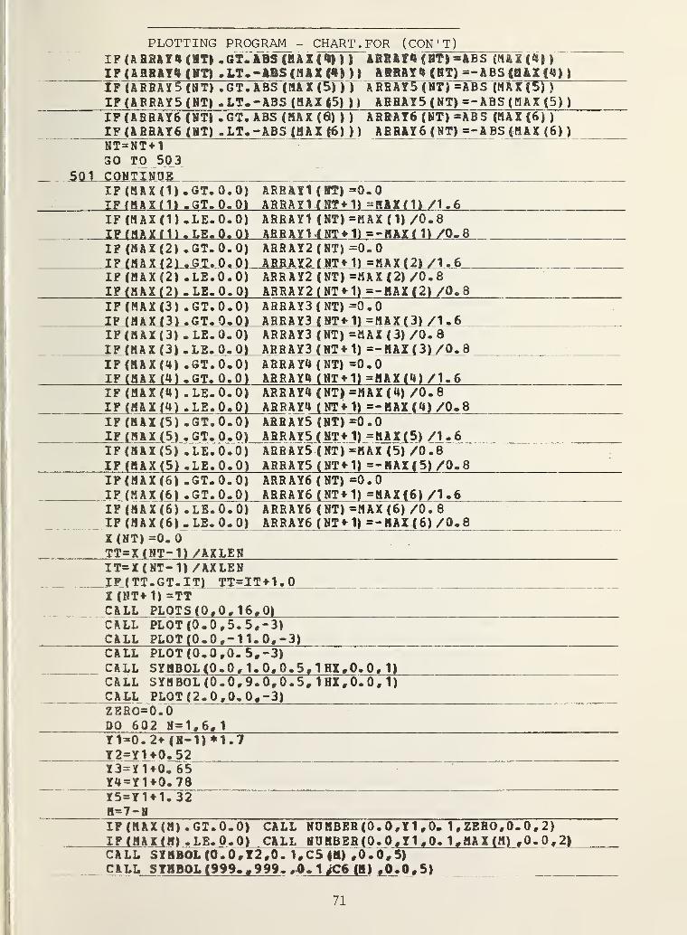
PLOTTING PROGRAM - CHART . FOR (CON'T)IF (ARRAY4 (HT) • GT.ABS (M A X (*1)} ) ABB AY4 CHT)=ABS(M A X ( 4 )

)

IF ( ARRAY4 (HT) .LT.-ABS (MAX (4)) ) ARRAY 4 (HT) =-ABS(a&X(4) )

IF (ARRAY5 (NT) .GT.ABS {MAX (5) )) ARRAYS (HT) =ABS (MAX{5) )

IF ( ARRAY5 (NT) •LT.-ABS (MAX $5) )> ARBAY5 (BT) =-ABS (MAX (5) )

IF (ARRAY6 (NT) .GT.ABS (MAX (6) ) ) ARRAY6 (NT) =ABS (MAX (6) )

IF (ARRAY6 (HT) .LT.-ABS (MAX (6) ) ) ARRAY 6 (NT) =-ABS (MAX (6) )

NT=NT+

1

SO TO 503501 CONTINUE I

~

IF (MAX (1 ) . GT. 0.0) ARRAY1 (HT) *0.0IF (MAXMl ,GT. 0.0) ARRAY! ( NT* 1) =HAX(1) /1.6IF (MAX(I).LE. 0.0) ARRAY1 (NT)=MAX(1) /0.8

___ IF (MAX (1) .LE.0.0) ARRAYl ( NT* 1) =-MAX(1) /O. 8

IF (MAX (2) .GT. 0.0) ARR AY2 ( NT) =0.

0

IF (MAX ( 2 ) . GT. 0 .0) AREA Y2 ( NT» 1 ) =MA X (2) / 1 . 6IF (MAX (2) .LE.0.0) ARRAY2 (NT) “MAX (2) /0.8IF (MAX (2) .LE.0.0) ARRAY2 ( NT» 1 )

=-MAX(2) /Q.8IF (MAX (3) .GT. 0.0) ARR AY3 ( NT) =0 .

0

IF (MAX (3) . G T. Q.O) AR R AY3 ( HT»1) =M A X(3) /I .6IF (MAX (3) .LE.0.0) ARRAY3 ( NT) =MAX (3) /0. 8

IF (MAX (3). LE.0.0) ARR AY 3 ( NT* 1) =- MAX (3)/0. 8

IF (MAX (4) .GT.0.0) AREA Y4 (NT) =0.0IF (MAX (4) .GT. 0.0) ABRAY4 (NT + 1) =HAX(4) /I. 6

IF (MAX (4 ) .LE.0.0) ARR AY4 ( NT) =M AX ( 4) /0.8IF CM A X (4) .LE. 0.0) ARR A Y4 (NT»1) =- MAX ( 4J /0. 8

IF (MAX (5) .GT.0.0) ARRAYS (NT) =0.0IF (M AX ( 5 ). GT.0.0) AR R AYS ( NT +1) =MAX(5 ) /I . 6

IF(MAX(5) .LE.0.0) ARRAYS (NT) =MAX (5) /0.8IF (MAX (5) .LE.0.0) ARRAYS (NT»1) =-MAX{5) /0.8IF(MAX(6) .GT.0.0) ARR AY6 ( NT) =0 .

0

IF (MAX (6) .GT.0.0) ABRAY6(NT+1) =MA X(6) /I. 6IF (MAX (6) .LE.0.0) ARRAY6 (NT) =MAX (6) /0.

8

IF (MA X (6 ) . LE.0.0) ARRAY6 ( NT» 1) =-MAX(6) /0. 8

X (NT) =0.

0

TT=X (NT-1) /AXLENIT=X ( NT- 1) /AXLENI F (TT . G T . I T1 _TT= I T + 1 . 0X (NT*- 1) =TT

___ C ALL PLOTS (0,0,16,0)CALL PLOT (0.0,5. 5,-3)CALL PLOT(Q. 0,-11. 0,-3)CALL PLOT (0.0,0. 5,-3)CALL SYMBOL

(

0. 0 , 1. 0,0.5, 1 HX,0.0, 1)CALL SYMBOL (0.0, 9. 0,0. 5, 1HX,0.0, 1)

CALL PLOT (2.0 ,0. 0,-3)ZERO=0.0DO 602 B= 1,6, 1

Y 1=0. 2 * (B-1) *1 .7Y2=Y1 »0. 52Y3=YUO. 65Y4=Y 1 >0. 7815*11*1. 32M=7-

B

IF (MAX(M) .GT.0.0) CALL NUMBER (0. 0 , Y 1 , 0. 1 , ZEBO,0. 0, 2)

_ IF (M A X(H) . LE. 0 .0) CALL .HU MBEB CO . 0, Y1 ,0. UMAX (H) ,0.0 ,2)CALL SYMBOL (0.0,12,0. 1,65*0) ,0.0,5)CALL SYMBOL (999., 999 . ,0 .1 jC6(M) ,0.0,5)

71

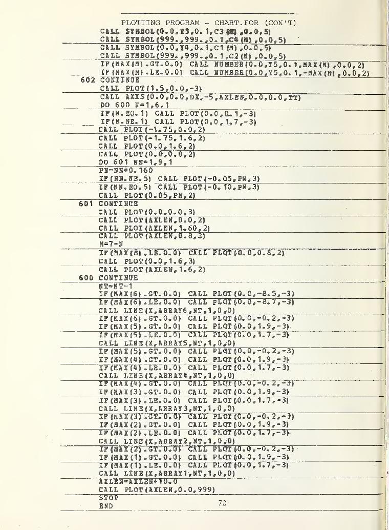
PLOTTING PROGRAM - CHART . FOR (CON'T)cm SXBBCL(O.0,f3,O. Iff C3 mCALL STBBOLC999, # 999.,Q, 1^C» (8) ,Q.0„S1CALL SYMBOL (0.0, Y4,Q. 1, Cl (M) ,0.0,5)CALL SYM BOL (999. ,999. ,0. 1 ,C2 (H) ,0.0,5)IF(HAX|H) .GT.0.0) CALL NUMBEB(0.0,Y5,0.i,MAX(M),0.,0,2)~IF (MAX(M) .LE.0.0) CALL HUMBEB(0.0,Y5,0. 1,-MAX (M>) ,0.0,2)

602 CONTINUECALL PLOT (1.5,0. 0,-3)CALL AXIS (0.0 ,0. 0,DX,-5 , AXLEN, 0. 0,0. 0 , TT)DO 600 H- 1 , 6,

1

IF (N. EQ. 1) CALL PLOT (0.0 ,G« 1 ,-3)IF ( M. MB. 1 ) CALL PLOT (0.0, t.7,-3)CALL PLOT (-1.7 5,0. 0,2) _CALL PLOT (-1.75, 1.6,2)CALL PLOT (0.0, 1.6,2)CALL PLOT (0.0,0. 0, 2)

DO 601 Ni« 1, 9 ,

1

" pfsN 8*0.160IF (NN. HE. 5) CALL PLOT (-Q. 05, PH , 3)

IF (NN. EQ. 5) CALL PLOT (-0. 10,PN,3)CALL PLOT (0.05, PH, 2)

601 CONTINUECA LL PLOT ( 0.0,0 . 0, 3)

CALL PLOT (IXLEiffO. 0,2)CALL PLOT (AXLEN, 1.60, 2)

CALL PLOT (AXLEN, 0.8, 3)

M-7-NIF(fillfM). LE. 0.0) CALL PLOT (0. 0,0. 8,2)CALL PLOT(0. 0, 1.6,3)CALL PLOT (AXLEN, 1.6,2)

600 CONTINUENT=NT-1IF (MAX (6) .6T.0.0) CALL PLOT (0. 0,-8* 5,-3)IFCHAXfSI .LE.0.0) CALL PLOT (.0. 0 ,-8777^1CALL LINE (X, ARRAYS , NT,1 » 0 ,0)IF ( H A X ( 6 1 . GT . 0 . 0 ) CA LL PLOT §0. 0 ,-0. T9 -3)IF(MAX(5). GT. Q® Q) CALL PLOT (0. 0 , 1 . 9 , - 3)

IF (MAX (5) .LE.0.0) CALL PLOT (0.0, 1.7, -3)CALL LINE (X, ARRAYS, NT, 1,0*0)IF (MAX (5) ®GT. 0.0) CALL PLOT (-0. 0,^5*. 2,-3)“IP(HAX(4) .GT.0.0) CALL PLOT (0.0, 1.9, -3)IF(MAX(4) .LE.0.0') CALL PLOT (0.0, 1.7,- 3)

CALL LINE (X, AREAY4, NT, 1 ,0,0)IF (MAX (4) • GT. 0.0) CALL PLOT (0. 0,-0. 2,-3)IF (HAX(3) .GT.0.0) CALL PLOT (0. 0 , 1. 9,-3)IF(HAX(3) .LE.0.0) CALL PLOT §0. 0,1.7, -3)

CALL LINE(X,ABRAY3,MT, 1,0,0)IF (MAX(3) .GT7070) CALL PLOT (G7G7-0. 2,-3)IF (MAX (2) . GT. 0.0) CALL PLOT (0.0, 1.9 , -3)

IFlBAX (2) .LE.0.0) CALL PLOT (0. 0 , 1® 7, -TFCALL LINE (X, ABBAY2, NT, 1 , 0 *?0)

IF (MAX (2) .GT. 0.0) CALL PLOT (0. 0 ,”07T7-T)IF (MAX (.1) .GT.0.0) CALL PLOT §0. 0 , 1. 9, -3)IF (MAX (1) .LE.0.0) CALL PLOT |0.0, 1.7,-3)CALL LIME (X, ARRAU, NT, 1,0,0)

" AXLEN- AXLEH4- 10.0CALL PLOT (AXLEN,0. 0,999)STOPEND 72

APPENDIX

GLOSSARY OF PROGRAM CONSTANTS AND VARIABLES

73

GLOSARY OF PROGRAM CONSTANTS AND VARIABLES

SYMBOL DESCRIPTION UNIT

ABAR Average acceleration over TAIL mph/sec

ABM Maximum allowable battery discharge

current

.

amp

ABT Battery current. amp

ABTAVE Average battery current over TAU. amp

ABT1 Previous battery current. amp

AC Charging equation factor (regeneration)

.

—ACC Acceleration

.

mph/sec

ACC1 Previous acceleration. mph/sec

ACCM Maximum acceleration. mph/ sec

ACHG Charging current (recharge)

.

amp

AF Vehicle Frontal area. ft 2

AH Ampere-hours removed from battery. amp -hr

AHF Ampere-hour factor. —AHR Rated battery capacity (C5) . amp -hr

AIC Charging current (regeneration). amp

AI CM Maximum charging current (recharge)

.

amp

AIO Offset current in charging voltage

equat ion

.

amp

AJERK Jerk rate. mph/sec

AJERKR Maximum jerk rate. mph/sec 2

AMASS Equivalent vehicle accelerating mass. g-lb

AMP Traction motor armature current. amp

AMPM Maximum traction motor armature current. amp

AMPMG Maximum traction motor current on grade. amp

AMPMO Maximum traction motor current -normal

.

amp

ANC Number of cells in battery —BC Charging equation factor (regeneration)

.

—CAP Battery capacity at current ABT amp -hr

CAY Excitation constant. volts/rpm

CAYA Coefficient in battery capacity equation. hr

CAYB Constant in battery capacity equation. hr

CAY C Factor in charging equations

74

GLOSSARY OF PROGRAM CONSTANTS AND VARIABLES (CONTINUED)

SYMBOL DESCRIPTION UNIT

CAYD Coefficient in discharge equation. volt /cell

CAY I Excitation factor-current. volt / rpm

CAYV Excitation factor- voltage

.

volt /rpm

CAYO Excitation limit. volt /rpm

CAY OA Excitation 1 imit -accelerat ion

.

volt /rpm

CAY OD Excitation limit-deceleration. volt /rpm

CAYOG Excitation limit on grade volt' / rpm

CC Charging equation factor (regeneration). —CHGTIM Recharge time. min

.

CM Exponent in discharge equation. —CN Exponent in battery capacity equation. —CR Coefficient of rolling resistance. lbf / lbm

Cl, C2 Factors in excitation equation. —CIO Battery capacity at 10 hour rate. amp -hr

DD Depth of discharge (AHR base)

.

pu

DECEL Deceleration limit. mph/ sec

DELAH Ampere-hour increment. amp -hr

DELI Discharge current increment. amp

DWELL Dwell time at stop. sec

EBAT Energy removed from battery. kw - hr

EC Battery charging equation constant. volts/cell

ECHG Energy input to battery from charger. kw- hr

EFFBAT Battery efficiency. pu

EG Battery gassing voltage volt /cell

EPM Specific power to battery. kw-hr/mi

EPM1 Specific power to wayside charging

station

.

kw-hr/mi

ETACHG Wayside charging station efficiency. pu

ETAG Rear end efficiency. pu

EO Open circuit battery voltage. volt /cell

G (25 , 2) Array of grade data. —GEE Acceleration due to gravity. mph/ sec

75

GLOSSARY OF PROGRAM CONSTANTS AND VARIABLES (CONTINUED)

SYMBOL DESCRIPTION UNIT

GRADE Roadway grade. rad

HW Headwind (enroute component)

.

mph

I, II Stop indices. —IAC Air conditioning control code. —IDC Driving cycle selection code. —IND Power limited mode and recharge index. —INI Initialization by-pass code. —IOF Output file selection code. —11,12 Output control codes. —ISW Stopping logic control code. —IWC Output write command code. —JG Grade index. —JM Route length mile index. —KG Grade index.

NP Number of passengers. —NT Number of stops per mile. —PAC Air conditioning compressor power. kw

PAIR Average air compressor load. kw

PAUX Auxiliary power load. kw

PBAUX Battery auxiliary power. kw

PBAVE Average battery power over TAU. kw

PBB Battery power. kw

PBC Average battery charger load. kw

PB1 Previous battery power. kw

PCBLO Air conditioning condenser blower. kw

PCHG Battery charging power. kw

PCUL Power conditioning unit loss. kw

PECBLO Environmental control blower. kw

PF Friction braking power. kw

PG Gassing power limit. kw

PHIR Route direction. deg

PHI W Wind direction. deg

76

GLOSSARY OF PROGRAM CONSTANTS AND VARIABLES (CONTINUED)

SYMBOL DESCRIPTION UNIT

PLTG Lighting power. kw

PS Traction motor shaft power. kw

PS1 Demanded value of PS. kw

PSMA Maximum shaft power - accelerat ion

.

kw

PSMD Maximum shaft power deceleration. kw

PTBLO Traction motor blower power. kw

PTF Traction motor field power. kw

PTMA Traction motor air-gap power. kw

PTMB Traction motor bearing loss. kw

PTMI Traction motor iron loss. kw

PTMI1 Updated value of PTMI. kw

PTMIN Traction motor armature circuit input. kw

PTML Total traction motor losses. kw

PTMW Traction motor windage loss. kw

PW Propulsion power. kw

Q Exponent in charging equation. —RATIO Reduction gear ratio. —RB Battery resistance in discharge

equation

.

ohm

RPM Traction motor speed. rpm

RTMA Traction motor armature resistance. ohm

S Distance travelled. mi

SB State of discharge. pu

SBO Initial state of discharge. pu

SC State of discharge in charging

equation

.

pu

SN Location of next stop. mi

SR Route length. mi

SS Stop spacing. mi

STAB Location of brake initiation point. mi

TA Aerodynamic drag. lb

TAU Computing interval. sec

77

GLOSSARY OF PROGRAM CONSTANTS AND VARIABLES (CONTINUED)

SYMBOL DESCRIPTION UNIT

TAU1 Nominal value of TAU. sec

TAUMU Make-up time. sec

TD Total drag force. lb

TF Tire factor. rpm/mph

TG Grade drag. lb

THETA Time from start to run. sec

TIM Output clock time. sec

TIMX Output interval. sec

TMIN Total time of run. min

TN Net accelerating thrust. lb

TNI Jerk limited thrust increment. lb

TP Tractive effort desired. lb

TR Rolling resistance drag. lb

TS Stopping clock. sec

T1 Time to completion of onset. sec

T2 Time to completion of constant

decelerat ion

.

sec

T3 Time to completion of flair. sec

T 4 Time to completion of dwell. sec

V Vehicle speed. mph

VI Previous vehicle speed. mph

VB Brush drop. volt

VBAR Average vehicle speed over TAU. mph

VBAT Battery terminal voltage. volt

VC Cruise speed. mph

VCHG Charging voltage. volt

VKE Vehicle kinetic energy. lew - h r

VOLT Traction motor input voltage. volt

VOLTM Maximum traction motor input voltage. volt

VOLTMA Maximum traction motor input voltage-

accelerat ion

.

volt

78

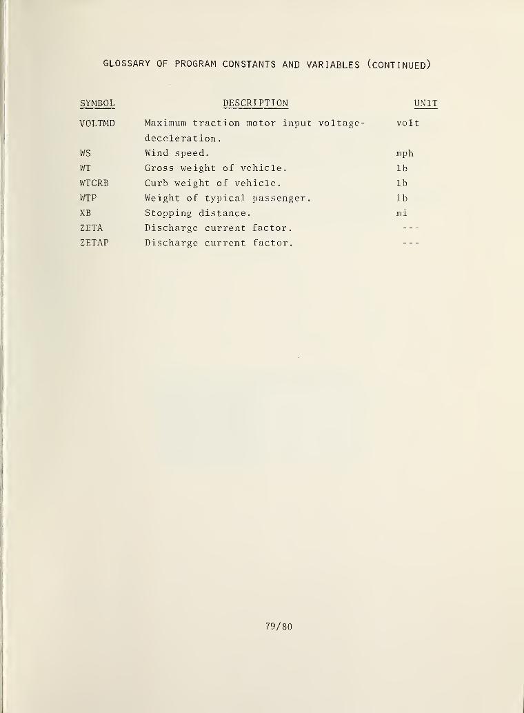
GLOSSARY OF PROGRAM CONSTANTS AND VARIABLES (CONTINUED)

SYMBOL DESCRIPTION UNIT

VOLTMD Maximum traction motor input voltage-

deceleration .

volt

WS Wind speed. mph

WT Gross weight of vehicle. lb

WTCRB Curb weight of vehicle. lb

WTP Weight of typical passenger. lb

XB Stopping distance. mi

ZETA Discharge current factor. —ZETAP Discharge current factor. —

79/80

REFERENCES

1. Larson, G.S. and H. Zuckerberg, Flywheel/Diesel Hybrid Power

Drive: Urban Bus Vehicle Simulation , U.S. Department of

Transportation, Urban Mass Transportation Administration,

Washington DC, Final Report, UMTA-MA- 06 - 0044 - 78 - 1 , May 1978.

2. Larson, G. and H. Zuckerberg, Diesel Bus Performance Simulation

Program , U.S. Department of Transportation, Urban Mass Trans-

portation Administration, Washington DC, Final Report,

UMTA-MA- 06-0044-79-1, April 1979.

I

n “no o7} -i

2 3 l

COi 00 '

i> :s i—1

pi

33 o H — O -Z 1—

*

5 o - h r Z X>H s m j> r"—

i •

nO T1 5 Xi H m jo

r —0 '—

' JO i

*c;

• —i•

8 S d ->/- jd 2 -~p

110 copies

OFFICIAL

BUSINESS

PENALTY

FOR

PRIVATE

USE.

«300

9 9> o9 v>H H£ >* £H >O 2"n O

9 pn

>2 ^fir 99 >

§ 6