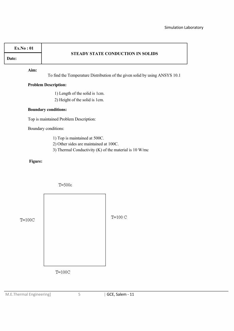
Simulation Laboratory M.E.Thermal Engineering] 5 | GCE, Salem - 11 Ex.No : 01 STEADY STATE CONDUCTION IN SOLIDS Date: Aim: To find the Temperature Distribution of the given solid by using ANSYS 10.1 Problem Description: 1) Length of the solid is 1cm. 2) Height of the solid is 1cm. Boundary conditions: Top is maintained Problem Description: Boundary conditions: 1) Top is maintained at 500C. 2) Other sides are maintained at 100C. 3) Thermal Conductivity (K) of the material is 10 W/mc Figure:

Welcome message from author
This document is posted to help you gain knowledge. Please leave a comment to let me know what you think about it! Share it to your friends and learn new things together.
Transcript
Simulation Laboratory
M.E.Thermal Engineering] 5 | GCE, Salem - 11
Ex.No : 01STEADY STATE CONDUCTION IN SOLIDS
Date:
Aim: To find the Temperature Distribution of the given solid by using ANSYS 10.1
Problem Description:
1) Length of the solid is 1cm.2) Height of the solid is 1cm.
Boundary conditions:
Top is maintained Problem Description:
Boundary conditions:
1) Top is maintained at 500C.2) Other sides are maintained at 100C.3) Thermal Conductivity (K) of the material is 10 W/mc
Figure:

Simulation Laboratory
M.E.Thermal Engineering] 5 | GCE, Salem - 11
PROCEDURE:STARTING ANSYS: Click on ANSYS 10.1 in the programs menu
MODELLING THE STRUCTURE:1. Go to the ANSYS main menu2. Create geometry.
Pre-processor >Modeling >create>Areas>Rectangle>By 2 corners>X=0,Y=0.Width =1,Height =1
ELEMENT PROPERTIESSELECTING ELEMENT TYPE:
Define the type of elementPre-processor >element Type >Add //edit/Delete...>click `Add` >select Thermal mass
solid, Quad 4 Node 55
Element material properties Pre processor > Material props> Material Modes > Thermal > conductivity>Isotropic > KXX =10 (Thermal conductivity)

Simulation Laboratory
M.E.Thermal Engineering] 5 | GCE, Salem - 11
MESHINGDIVIDING THE CHANNEL INTO ELEMENTS:
Mesh Size Preprocessor> Meshing > size cntrls > Manual size > Areas > All Areas > 0.05 MeshMesh
Pre processor > Meshing > Mesh > Areas > Free > Pick AllBOUNDARY CONDITIONS AND CONSTRAINTS
Define Analysis Type
Solution > Analysis Type > New Analysis > steady state
Apply ConstraintsSolution > Define Loads > Apply> Thermal > Temperature > On Lines
Apply temperature as per the figure
SOLUTION
Solve the system
Solution > solve > current LS>Ok
POST PROCESSING
Plot the Temperature distribution
General post proc > Plot results > Contour lot > Nodal Solu… > DOF solution,Temperature TEMP.

Simulation Laboratory
M.E.Thermal Engineering] 5 | GCE, Salem - 11

Simulation Laboratory
M.E.Thermal Engineering] 5 | GCE, Salem - 11
TEMPERATURE DISTRIBUTION
RESULTS:
Thus the temperature distribution of the given solid is determined.
Ex.No : 02STEADY STATE CONDUCTION IN SOLIDS
Date:
Aim:
To find the temperature distribution of the given solid by using ANSYS 10.1
Problem Description:
1) Length of the solid cylinder is 5cm.2) Diameter of the solid cylinder is 2cm.
Boundary condition:
1) Wall temperature is 20 C.2) Base of the rod is 320 C.3) Convection Co-efficient of the wall is 100 W/m2 C4) Rod tip is insulated.
Figure:

Simulation Laboratory
M.E.Thermal Engineering] 5 | GCE, Salem - 11
PROCEDURE:
STARTING ANSYS:
Click on ANSYS 10.1 in the programs menu
MODELLING THE STRUCTURE:
1) Go to the ANSYS Main Menu2) Create geometry
Pre-processor > Modeling > create > Volume > Cylinder > Solid Cylinder > Radius=1 , Depth = 5.
ELEMENT PROPEERTIES
SELECTING ELEMENT TYPE:
Define the Type of element
Preprocessor > Element type > Add/Edit/Delete...> click `Add` > select ThermalMass Solid, 20 nodes 90.
Material properties
Preprocessor > Material Props > Material models > Thermal Conductivity >Isotropic > kxx =50 (Thermal conductivity)
MESHING
DIVIDING THE SHANNEL INTO ELEMENTS:
Mesh size

Simulation Laboratory
M.E.Thermal Engineering] 5 | GCE, Salem - 11
Pre-processor > Meshing > Size cntrls > Manual size > Areas > All Areas > 0.05
Mesh
Pre processor > Meshing > Mesh > Volume > Free > Pick All
BOUNDARY CONDITIONS AND CONSTRAINTS
Analysis Type
Solution > Analysis Type > New Analysis > steady state
Constraints
Solution > Define Loads > Apply
Thermal > Temperature > On lines
Fill the window in as shown to constraint the side to constant temperature of 320
Solution > Define Loads > Apply
Thermal > Convection > On areas
Fill the window in as shown to constrain the side to film coefficient of 100 and bulk Temperature of 20.(As shown in Figure)
Solution > Define Loads > Apply
Thermal > Convection > On areas
Fill the window in as shown to constrain the side to film coefficient of 0 and bulkTemperature of 0. .(As shown in Figure)
SOLUTION
Solve the system
Solution > solve > Current LS
SOLVE
POST PROCESSING

Simulation Laboratory
M.E.Thermal Engineering] 5 | GCE, Salem - 11
Plot the temperature distribution
General Postproc > Plot Results > Contour plot > Nodal Solu… > DOF solution,Temperature TEMP

Simulation Laboratory
M.E.Thermal Engineering] 5 | GCE, Salem - 11
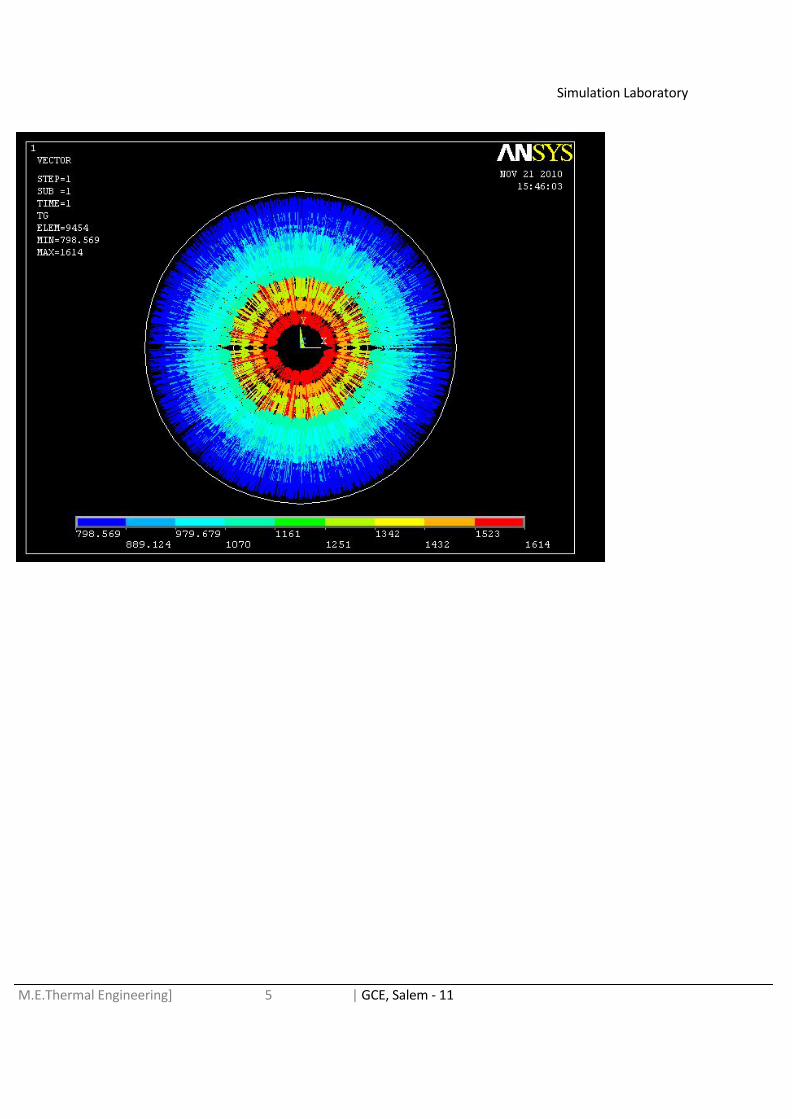
TEMPERATURE DISTRIBUTION
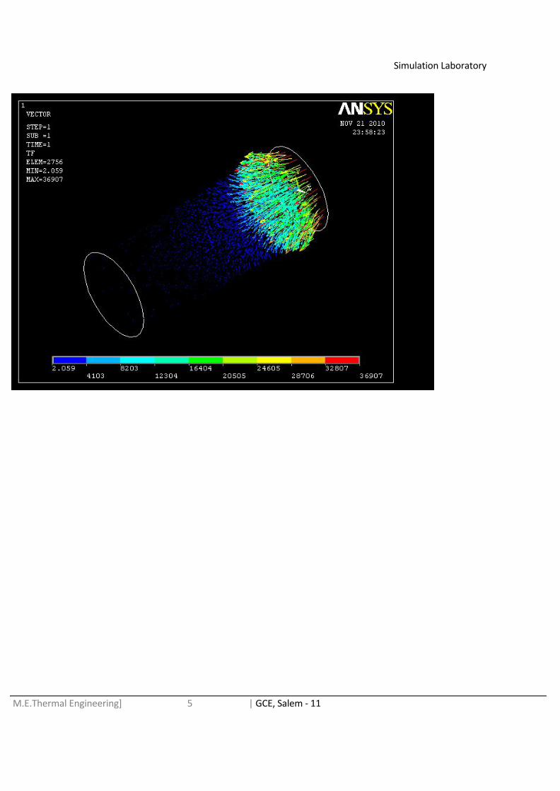
VECTOR PLOT:
Now go to General Postproc > Plot Results > Vector Plot > Predefined and selectVelocity.
Simulation Laboratory
M.E.Thermal Engineering] 5 | GCE, Salem - 11

Simulation Laboratory
M.E.Thermal Engineering] 5 | GCE, Salem - 11
RESULTS:
Thus the temperature distribution of the given solid cylinder is determined.
Ex.No : 03STEADY STATE RADIATION IN SOLIDS
Date:
Aim :
To find the temperature distribution of the given solid by using ANSYS 10.1
Problem Description:
1. Length of the strip is 2cm.2. Height of the strip is 1cm.
Boundary condition:
1. Left and Right side temperature is 900 C and Emissive is 0.7.2. Convection Co-efficient of the top is 100W/m2C and Bulk temperature is 50C.3. Stephen Boltze` man constant is 5.67e-8W/m2K4.
Material properties:
1. Thermal conductivity is 3W/m C.2. Density is 1600 kg/m3.3. Specific heat is 800 J/kg C.

Simulation Laboratory
M.E.Thermal Engineering] 5 | GCE, Salem - 11
Figure:
PROCEDURE:
STARTING ANSYS:
Click on ANSYS 10.1 in the programs menu
MODELLING THE STRUCTURE:
1. Go to the ANSYS Main Menu2. Create geometry
Pre-processor > Modeling > create > Areas > Rectangle > By 2 Corners > X =0, Y=0,Width=2, Height = 1.
ELEMENT PROPEERTIES
SELECTING ELEMENT TYPE:
Define the Type of element
Preprocessor > Element type > Add/Edit/Delete...> click `Add` > select ThermalMaterial properties
Preprocessor > Material Props > Material models > Thermal >Conductivity>Isotropic > kxx =3 (Thermal conductivity)
Specific heat =800Density =1600.
MESHING

Simulation Laboratory
M.E.Thermal Engineering] 5 | GCE, Salem - 11
DIVIDING THE SHANNEL INTO ELEMENTS:
Mesh size
Pre-processor > Meshing > Size cntrls > Manual size > Areas > All Areas > 0.05
Mesh
Pre processor > Meshing > Mesh > Areas > Free > Pick All
BOUNDARY CONDITIONS AND CONSTRAINTS
Analysis Type
Solution > Analysis Type > New Analysis > steady state
Constraints
Solution > Define Loads > Apply
Thermal > Temperature > On lines
Fill the window in as shown to constraint the side to constant temperature of 900
Solution > Define Loads > Apply
Thermal > Convection > Online
Fill the window in as shown to constrain the side to film coefficient of 100 and bulk Temperature of 50.
Solution > Define Loads > Apply
Thermal > Radiation > Online
Fill the window in as shown to constrain the side to a emissivity of 0.7 and enclosure no is2.
Preprocessor > Radiation opts > solution opt
Fill the window in as shown to constrain the side to a Stephen Boltze man constant of 5.67e-8.7 and enclosure no is 2.
Main menu > Radiation Opt > Matrix method > Other settings
Fill the window in as shown to constrain the side to a Stephen Boltze man constant of 5.67e-8.7 And type of geometry is 2D.

Simulation Laboratory
M.E.Thermal Engineering] 5 | GCE, Salem - 11
SOLUTION
Solve the system
Solution > solve > Current LS
SOLVE
POST PROCESSING
Plot the temperature distribution
General postproc > Plot Results > contour plot > Nodal Solu… > DOF solution,Temperature TEMP

Simulation Laboratory
M.E.Thermal Engineering] 5 | GCE, Salem - 11
TEMPERATURE DISTRIBUTION
VECTOR PLOT:
Now go to General Postproc > Plot Results > Vector Plot > Predefined and select
Thermal flux

Simulation Laboratory
M.E.Thermal Engineering] 5 | GCE, Salem - 11

Simulation Laboratory
M.E.Thermal Engineering] 5 | GCE, Salem - 11
RESULTS:
Thus the temperature distribution and thermal flux of the given strip is determined.
Ex.No : 04COMBINED CONDUCTION AND CONVECTION IN SOLIDS
Date:
Aim:
To find the Temperature distribution of the given solid by using ANSYS 10.1
Problem Description:
Dimensions:
1. Length of the fin is 8 cm.2. Width of the fin is 2cm.
Boundary Conditions:
1. Wall temperature is 20 C2. Base of the rod is 300 C3. Convection Co-efficient of the wall is 40 W/m2C.
Figure
Simulation Laboratory
M.E.Thermal Engineering] 5 | GCE, Salem - 11
PROCEDURE;
STARTING ANSYS:
Click on ANSYS 10.1 in the program menu.
MODELLING THE STRUCTURE:
1) Go to the ANSYS main menu.2) Create geometry.
Preprocessor > Modeling > create > Areas > Rectangle > By 2 corners > X=0, Y=0,Width =8, Height=2.
ELEMENT PROPERTIES
SELECTING ELEMENT TYPE
Define the type of element
Preprocessor > Element Type > Add/Edit/Delete >click `Add` > select
Thermal Mass Solid, Quad 4Node 55
Element material properties
Preprocessor> Material props > Material Models > Thermal conductivity>Isotropic > KXX = 1 (Thermal conductivity)
MESHING

Simulation Laboratory
M.E.Thermal Engineering] 5 | GCE, Salem - 11
DIVIDING THE CHANNEL INTO ELEMENTS:
Mesh Size
Preprocessor > Meshing > size cntrls > Manual size > Areas > All areas > 0.05 Mesh
Preprocessor > Meshing > Mesh > Areas > Free > Pick all
BOUNDARY CONDITIONS AND CONSTRAINTS
Define Analysis Type
Solution > Analysis Type > New Analysis > steay state Apply Constraints
Solution > Define Loads > Apply
Thermal > convection> Online lines
Fill the window in as shown to constrain the strip to a film coefficient of 40 and bulktemperature of 20.
SOLUTION
Solve the system
Solution > solve > current LS
SOLVE
Simulation Laboratory
M.E.Thermal Engineering] 5 | GCE, Salem - 11
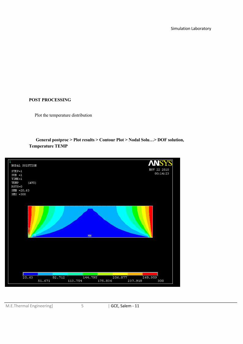
POST PROCESSING
Plot the temperature distribution
General postproc > Plot results > Contour Plot > Nodal Solu…> DOF solution,Temperature TEMP

Simulation Laboratory
M.E.Thermal Engineering] 5 | GCE, Salem - 11
TEMPERATURE DISTRIBUTION
RESULT:
Thus the temperature distribution of the given Strip is determined.
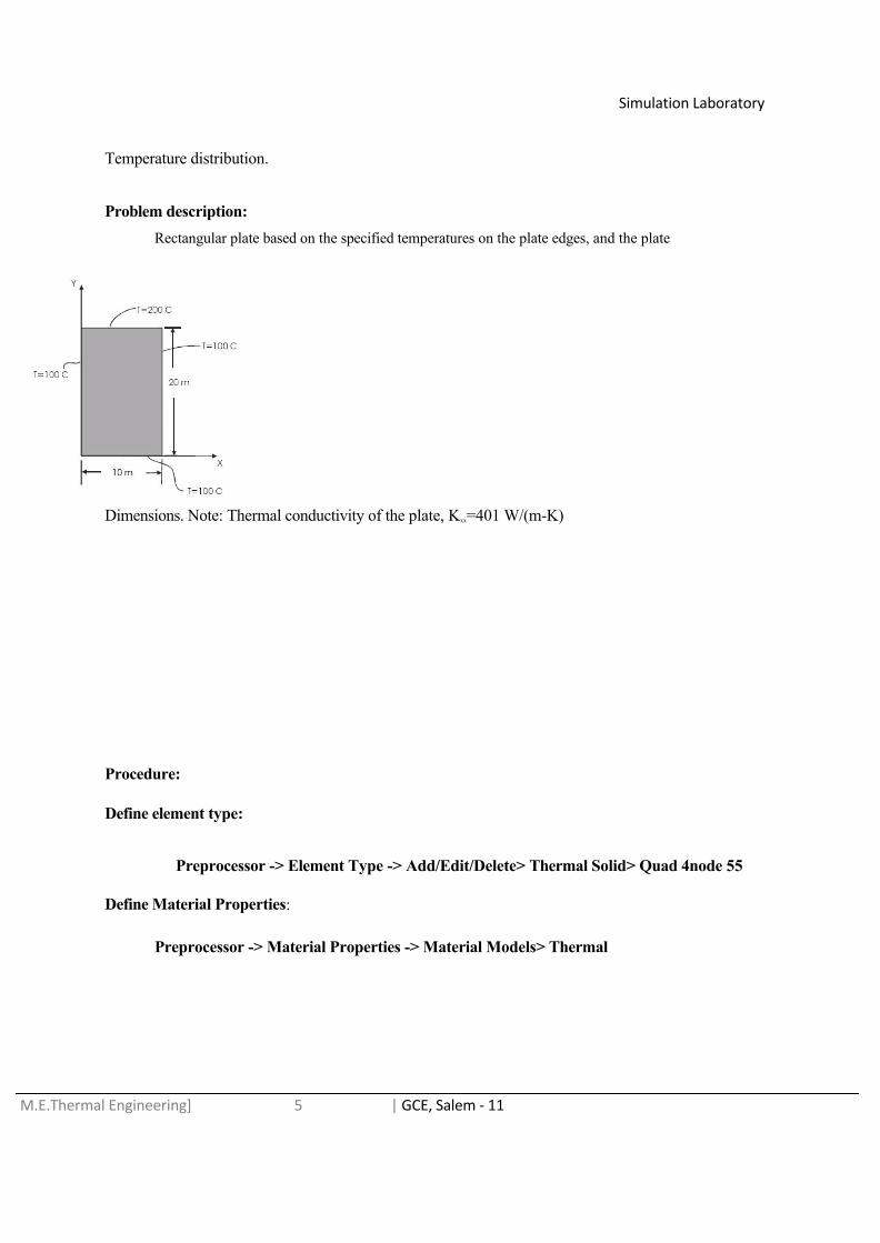
Ex.No : 05CONDUCTION HEAT TRANSFER IN A PLATE
Date:
Aim :
To solve the 2-D heat conduction problem below, using ANSYS. And find the
Simulation Laboratory
M.E.Thermal Engineering] 5 | GCE, Salem - 11
Temperature distribution.
Problem description:Rectangular plate based on the specified temperatures on the plate edges, and the plate
Dimensions. Note: Thermal conductivity of the plate, Kxx=401 W/(m-K)
Procedure:
Define element type:
Preprocessor -> Element Type -> Add/Edit/Delete> Thermal Solid> Quad 4node 55
Define Material Properties:
Preprocessor -> Material Properties -> Material Models> Thermal

Simulation Laboratory
M.E.Thermal Engineering] 5 | GCE, Salem - 11
ModelingPreprocessor -> Modeling-> Create -> Areas -> Rectangle -> By DimensionsFill in the fields, (X1, X2) as 0, 10 & (Y1, Y2) as 0, 20 and then click “OK”.
Specify mesh density controls.
We will specify numbers of element divisions along lines. Choose: Preprocessor -> -Meshing- Size Controls -> Manual Size -> Lines-> Picked Lines
The picking menu (below left) appears. On the graphics window, click on the bottomHorizontal line (this is one of the 10 meter lines), to highlight it. Then, click “OK” in thePicking menu. Then, the “Element Size” menu (below right) appears. Enter “10” for“NDIV”, as shown, then click “OK”. Now, repeat the above process to specify 20 divisionsalong either of the vertical lines.
Mesh the rectangle to create nodes and elements.Preprocessor -> Meshing -> Mesh -> Areas -> Mapped -> 3 or 4 Sided
A picking menu appears. Select “Pick All”. The rectangle will be meshed.
Solution:
Apply temperatures around the edges:Solution -> Define Loads-> Apply -> Thermal-> Temperature -> On Lines
A picking menu appears. Highlight the two vertical lines (the 20 meter lines), which have atemperature of 100 C, then click on “OK” in the picking menu. The box on the next page Appears. Highlight “TEMP” for “DOFs to be constrained”, and enter “100” for “VALUE”.Repeat the above process to apply the 100 C temperature to the bottom horizontal line, but inthis case, choose “Yes” for “Apply TEMP to endpoints?” Repeat the process once more, toapply the 200 C temperature to the top horizontal line, but in this case, choose “No” for“Apply TEMP to endpoints?”
Now, to address the fact that two corners do not have a specified temperature, as anApproximation, we will set the temperature at these to corners to 150 C.
Solution -> Define Loads-> Apply -> Thermal-> Temperature -> On Key points
A picking menu appears. Note that there are four “key points” in the model, one at each
Simulation Laboratory
M.E.Thermal Engineering] 5 | GCE, Salem - 11
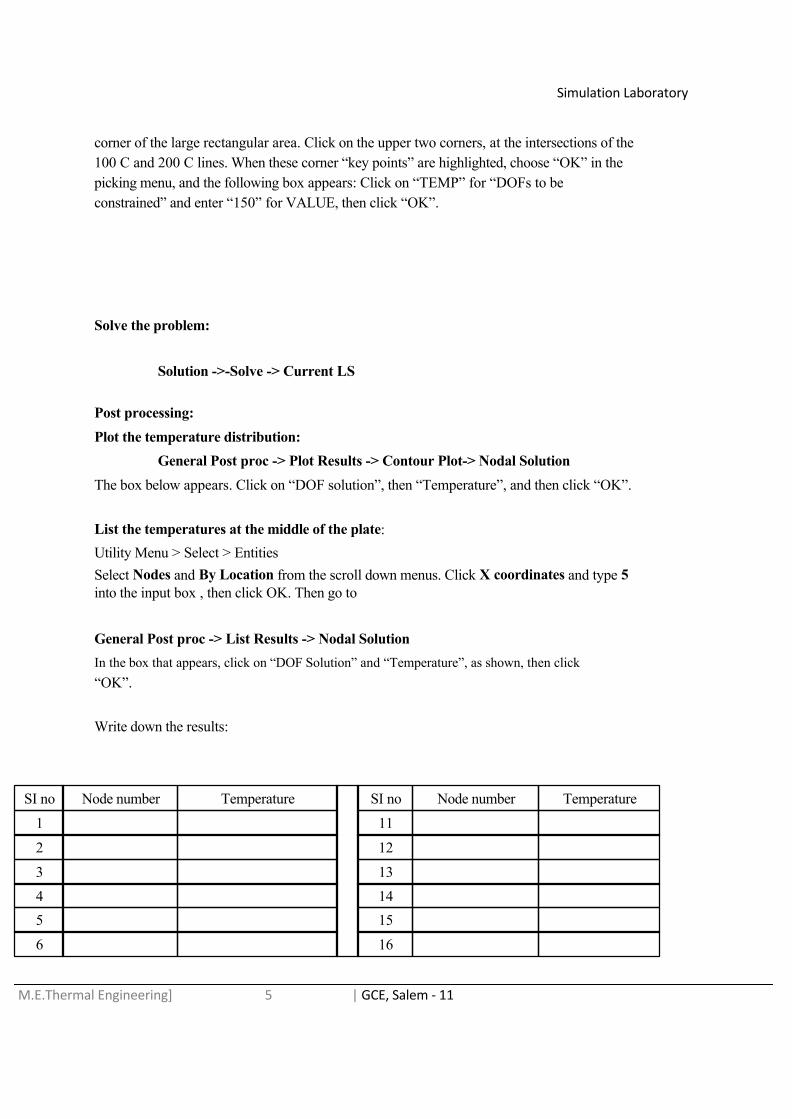
corner of the large rectangular area. Click on the upper two corners, at the intersections of the100 C and 200 C lines. When these corner “key points” are highlighted, choose “OK” in thepicking menu, and the following box appears: Click on “TEMP” for “DOFs to beconstrained” and enter “150” for VALUE, then click “OK”.
Solve the problem:
Solution ->-Solve -> Current LS
Post processing:Plot the temperature distribution:
General Post proc -> Plot Results -> Contour Plot-> Nodal SolutionThe box below appears. Click on “DOF solution”, then “Temperature”, and then click “OK”.
List the temperatures at the middle of the plate:Utility Menu > Select > EntitiesSelect Nodes and By Location from the scroll down menus. Click X coordinates and type 5into the input box , then click OK. Then go to
General Post proc -> List Results -> Nodal SolutionIn the box that appears, click on “DOF Solution” and “Temperature”, as shown, then click“OK”.
Write down the results:
SI no Node number Temperature SI no Node number Temperature
1 11
2 12
3 134 145 15
6 16

Simulation Laboratory
M.E.Thermal Engineering] 5 | GCE, Salem - 11
7 17
8 18
9 19
10 20

Simulation Laboratory
M.E.Thermal Engineering] 5 | GCE, Salem - 11
Plot Results
General postproc > Plot Results > contour plot > Nodal Solu… > DOF solution,Temperature TEMP

Simulation Laboratory
M.E.Thermal Engineering] 5 | GCE, Salem - 11
Result:
Thus the given 2-d heat conduction problem is solved using ansys. and the temperature
distribution within the rectangular plate, based on the specified temperatures on the plate edges, and the
plate dimensions was found.
Ex.No : 06 THERMAL ANALYSIS USING MIXED BOUNDARY CONDITIONS

Simulation Laboratory
M.E.Thermal Engineering] 5 | GCE, Salem - 11
Date:
Aim: To solve the 2-D heat conduction and convection problem below using ANSYS, and find the temperature
distribution.
Problem Description:
The Mixed Convection/Conduction/Insulated Boundary Conditions Example is constrained as shown in thefollowing figure (Note that the section is assumed to be infinitely long):
Procedure:Create geometry
Preprocessor > Modeling > Create > Areas > Rectangle > By 2 Corners > X=0, Y=0,Width=1, Height=1Define the Type of Element
Preprocessor > Element Type > Add/Edit/Delete... > click 'Add' > Select Thermal Mass Solid, Quad 4Node55ET, 1, PLANE55
Material Properties

Simulation Laboratory
M.E.Thermal Engineering] 5 | GCE, Salem - 11
Preprocessor > Material Props > Material Models > Thermal > Conductivity > Isotropic >KXX = 10This will specify a thermal conductivity of 10 W/m*C.Element
Mesh SizePreprocessor > Meshing > Size Cntrls > Manual Size > Areas > All Areas > 0.05
MeshPreprocessor > Meshing > Mesh > Areas > Free > Pick All
Solution Phase: Assigning Loads and SolvingDefine Analysis Type
Solution > Analysis Type > New Analysis > Steady-State
Apply Conduction ConstraintsIn this Problem, all 2 sides of the block have fixed temperatures, while convection occurs on the other 2 sides.
Solution > Define Loads > Apply > Thermal > Temperature > On LinesSelect the top line of the block and constrain it to a constant value of 500 C Using the same method, constrain the left side of the block to a constant value of 100 C
Apply Convection Boundary ConditionsSolution > Define Loads > Apply > Thermal > Convection > On Lines
Select the right side of the block.Fill in the window. This will specify a convection of 10 W/m2*C and an ambient temperature of 100 degrees Celsius. Note that VALJ and VAL2J have been left blank. This is because we have uniform convection across the line.Apply Insulated Boundary Conditions
Solution > Define Loads > Apply > Thermal > Convection > On Lines
Select the bottom of the block.Enter a constant Film coefficient (VALI) of 0. This will eliminate Convection through the side, thereby modeling an insulated wall. Note: you do not need to enter a Bulk (Or
ambient) temperature.
Solve the SystemSolution > Solve > Current LSSOLVE

Simulation Laboratory
M.E.Thermal Engineering] 5 | GCE, Salem - 11
Post processing:Viewing the ResultsPlot Temperature
General Post proc > Plot Results > Contour Plot > Nodal Solu ... > DOF solution, Temperature
Simulation Laboratory
M.E.Thermal Engineering] 5 | GCE, Salem - 11
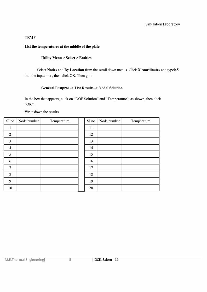
TEMP
List the temperatures at the middle of the plate:
Utility Menu > Select > Entities
Select Nodes and By Location from the scroll down menus. Click X coordinates and type0.5 into the input box , then click OK. Then go to
General Postproc -> List Results -> Nodal Solution
In the box that appears, click on “DOF Solution” and “Temperature”, as shown, then click“OK”.
Write down the results
SI no Node number Temperature SI no Node number Temperature
1 11
2 12
3 13
4 14
5 15
6 16
7 17
8 18
9 19
10 20

Simulation Laboratory
M.E.Thermal Engineering] 5 | GCE, Salem - 11

Simulation Laboratory
M.E.Thermal Engineering] 5 | GCE, Salem - 11
POST PROCESSING
Plot the temperature distribution
General postproc > Plot results > Contour Plot > Nodal Solu…> DOF solution,Temperature TEMP

Simulation Laboratory
M.E.Thermal Engineering] 5 | GCE, Salem - 11
Result:
Thus the given 2-D heat conduction and convection problem is solved using ANSYS.
And the temperature distribution within the component based on the specified temperatures
on the edges, and the dimensions, was found.

Simulation Laboratory
M.E.Thermal Engineering] 5 | GCE, Salem - 11
Ex.No : 07LAMINAR FLOW OVER FLAT PLATE
Date:
Aim:
To find the Temperature Distribution of the Laminar flow over flat plate.
Problem Description:
Dimensions:
1) Length of the plate is 1 m long.2) The flow area is 1 m * .25 m. .
Boundary conditions:
1) The velocity of the air at infinite distance from the plate is 0.5 m/s.2) Atmospheric pressure is assumed on all faces except the face where velocity is
input into the system.
Figure:

Simulation Laboratory
M.E.Thermal Engineering] 5 | GCE, Salem - 11
PROCEDURESTARTING ANSYS
1) Click on ANSYS 10.1 in the programs menuMODELING THE STRUCTURE: Click
Preprocessor>Modeling>Create>Areas>Rectangle->By2 Corners.
The width is 1 and the height is .25. Starting position is at (0,0).
The modeling of the problem is done
ELEMENT PROPERTIES
SELECTING ELEMENT TYPE:ClickPreprocessor>Element Type>Add/Edit/Delete...> Flotran CFD > Flotran 141
MESHING
DIVIDING THE CHANNEL INTO ELEMENTS:
Go to Preprocessor>Meshing>SizeCntrls>ManualSize>Lines>Picked Lines.
Select thetop and bottom lines (horizontal lines of the rectangle).In the window that comes up type
50 in the field for 'No. of element divisions'. Now Click OK.
Go to

Simulation Laboratory
M.E.Thermal Engineering] 5 | GCE, Salem - 11
Preprocessor>Meshing>SizeCntrls>ManualSize>Lines>Picked Lines.
Select the two vertical lines of the rectangle. In the window that comes up type 100 in the field for 'No. of
element divisions' and type 10 in the field for 'Spacing ratio'Now click OK
Go toPreprocessor>Meshing>Size Cntrls>ManualSize>Lines>Flip Bias. Select the left
line of the rectangle and click OK.
Now go to
Preprocessor>Meshing>Mesh>Areas>Free
Fluid Properties (air):
Go to Preprocessor>Flotran Set Up>Fluid Properties.
On the box, shown below, set the first 2 input fields to Air-Si. Then click on OK.
BOUNDARY CONDITIONS AND CONSTRAINTS
The boundary conditions in this problem are an imposed velocity over the plate, and
the no-slip condition on the plate itself.
To apply the imposed velocity ,go to
Preprocessor>Loads>DefineLoads>Apply>Fluid CFD>Velocity>On lines.
Pick the left edge and the top edge of the rectangle and Click OK. The following window comes up.
Enter0.5 in the VX field and0 in the VY and VZ fields. Make sure'Apply toendpoints' is set to Yes.
Then click OK. This number corresponds to the velocity of 0.5 meter per second of air flowing from
The left side and the assumption that thevelocity is equal to 0.5 far from the plate..
To set the no-slip condition on the plate, repeat the above procedure but this time set
the Velocity to ZERO for the bottom line of the rectangle. (VX=VY=0). This time
make sure 'Apply to endpoints' is set to Yes.
Now Atmospheric Pressure must be set for the right side of the rectangle.
Simulation Laboratory
M.E.Thermal Engineering] 5 | GCE, Salem - 11
To do this, select
Preprocessor>Loads>Define Loads>Apply>FluidCFD>Pressure DOF>On lines.
Click the right line and then OK. The following window will now appear.
Enter 0 for the constant pressure value for these faces and click OK. This sets the pressure to Atmospheric.
SOLUTION
Go to ANSYS Main Menu>Solution>Flotran Set Up>Execution Ctrl.
Go to Solution>Run FLOTRAN.
POST-PROCESSING
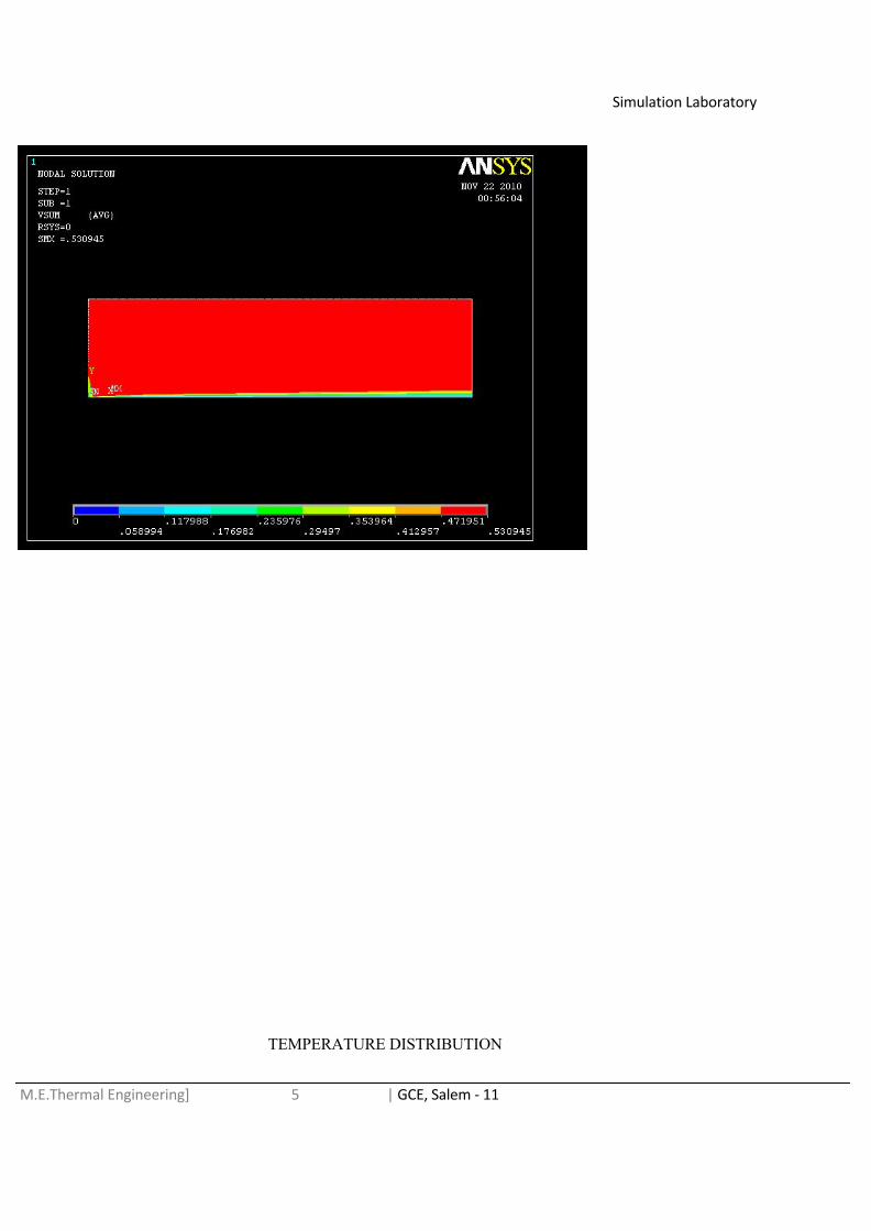
Plot the temperature distribution
General Postproc>Plot Results>Contour Plot>Nodal Solution.
Simulation Laboratory
M.E.Thermal Engineering] 5 | GCE, Salem - 11
TEMPERATURE DISTRIBUTION

Simulation Laboratory
M.E.Thermal Engineering] 5 | GCE, Salem - 11
VECTOR PLOT
Now go to General Postproc>Plot Results>Vector Plot>Predefined andselect Velocity. Enter a scale factor (VRATIO) of 0.4. The vector plot looks like this:

Simulation Laboratory
M.E.Thermal Engineering] 5 | GCE, Salem - 11
Simulation Laboratory
M.E.Thermal Engineering] 5 | GCE, Salem - 11
VECTOR PLOT
RESULT :
Thus the temperature distribution of the laminar flow over the flat plate is determined.

Simulation Laboratory
M.E.Thermal Engineering] 5 | GCE, Salem - 11
Ex.No : 08COMPOSITE WALL
Date:
Aim:
To find the Temperature distribution of the given composite wall by using ANSYS 10.1
Problem Description:
Dimensions:
1) Length = 3 m
2) Width = 3 m
3) Thickness of each Layer = 1 m
Boundary Conditions:
1) The left side of the block has a constant temperature of 400 K.
2) The right side of the block has convection (h=20 W/m-K ; T= 300 K)
3) The Al section generates heat at a rate of 200 W/m3
4) The He section absorbs heat at a rate of 175 W/m3
Figure

Simulation Laboratory
M.E.Thermal Engineering] 5 | GCE, Salem - 11
PROCEDURE:
STARTING ANSYS:MODELING THE STRUCTURE:
1) Go to the ANSYS main menu2) Create geometry
Preprocessor > Modeling > Create > Areas > Arbitrary > Through KPs . Length = 3m,Width =3m.
ELEMENT PROPERTIES
Aluminum(1stlayer): KAl= 235 W/m*K
Helium(2ndlayer): KHe= 0.1513 W/m*K
Copper(3rdlayer): KCu= 400 W/m*

Simulation Laboratory
M.E.Thermal Engineering] 5 | GCE, Salem - 11
1) Now that we’ve defined what material ANSYS will be analyzing, we have to definehow ANSYS should analyze our block.
2) Click Preprocessor>Element Type>Add/Edit/Delete... In the 'Element Types'window that opens click on Add... The following window opens:
3) Type 1 in the Element Type reference number.
4) Click on Thermal Mass>Solid and select Quad 8node 77. Click OK. Close the'Element Types' window.
5) Now we have selected Element Type 1 to be a Thermal Solid 8node Element.
6) This finishes the section defining how the part is to be analyzed.
7) Now we have selected Element Type 1 to be a Thermal Solid 8node Element.
8) This finishes the section defining how the part is to be analyzed.
SELECTING ELEMENT TYPE:
Define the Type of Element
Preprocessor > Element Type > Add/Edit/Delete…>click Add > Thermal Mass >Solid > select Quad8node 77.

Simulation Laboratory
M.E.Thermal Engineering] 5 | GCE, Salem - 11
Element material properties
Preprocessor > Material props> Material models > Thermal > conductivity >Isotropic.
1) Fill in 235 for Thermal conductivity. Click OK. This is the Thermal Conductivity of Al.
2) Now repeat the steps of clicking Thermal>Conductivity>Isotropic and then Defining the Thermal Conductivityas 0.1513 for the Model 2.
3) You have now defined the k value of Helium.
4) Define the last section and this time use K = 400. This is the Thermal Conductivity of Copper.
MESHING
DIVIDING THE CHANNEL INTO ELEMENTS:
1) Mesh size
Preprocessor > Meshing > Size controls > Manual size > Lines > All Lines. >0.05
Now go to Preprocessor>Meshing>Mesh Attributes>Default Attributes
2) Mesh
Preprocessor > Meshing > Mesh > Areas >Free
3) A popup window will appear on the left hand side of the screen. This window allows you to select the area to
be meshed.
4) Choose the 1starea and then click OK in the pop-up window. This both meshes the area and defines it as
Material 1. Material 1 (as you recall from before) was set to Aluminum originally by defining the k value of the
material as 235 W/m*K.
5) Now return to Preprocessor>Meshing>Mesh Attributes>Default Attributes. This time, select Material Number2 from the dropdown menu and click OK.
6) Once the pop-up window appears, select the middle layer and click OK.
7) Repeat this process of defining each layer as a different material for Material 3 and mesh it so that all threelayers have been meshed.
8) The block should now look like this when you are done meshing: (if you choose fit in the pan zoom rotatedialog)

Simulation Laboratory
M.E.Thermal Engineering] 5 | GCE, Salem - 11
BOUNDARY CONDITIONS AND CONSTRAINTS:
Constraints
Apply constant Temperature
Preprocessor > Loads > Define Loads > Apply > Thermal >Temperature > Online.
Enter 400 in the popup window as the set temperature for the left edge of the first section:
Apply Convection
Preprocessor > Loads > Define Loads > Apply > Thermal >Convection > Online
Apply Heat Generation and Heat Absorption
Preprocessor > Loads > Define Loads > Apply > Thermal >Heat General > Areas
Enter 200 W/m3for the generation and the hit ok.
Repeat this step for the second area but input -175 W/m3to imply absorption.
SOLUTION
Solve the system
Solution > Solve > Current LS
SOLVE

Simulation Laboratory
M.E.Thermal Engineering] 5 | GCE, Salem - 11
POST PROCESSING
Now go to General Post processing > Plot Results >Contour Plot > Nodal
Solution.> DOF solution > Temperature.

Simulation Laboratory
M.E.Thermal Engineering] 5 | GCE, Salem - 11
TEMPERATURE DISTRIBUTION
VECTOR PLOT:
Now go to General Postproc > Plot Results > Vector Plot > Predefined and select
Thermal flux

Simulation Laboratory
M.E.Thermal Engineering] 5 | GCE, Salem - 11

Simulation Laboratory
M.E.Thermal Engineering] 5 | GCE, Salem - 11
RESULT:
Thus the temperature distribution of the composite wall is determined.

Simulation Laboratory
M.E.Thermal Engineering] 5 | GCE, Salem - 11
Ex.No : 09STEADY STATE CONVECTION IN FLUIDS
Date:
Aim:
To plot the velocity distribution of the flow of air over an infinite cylinder.
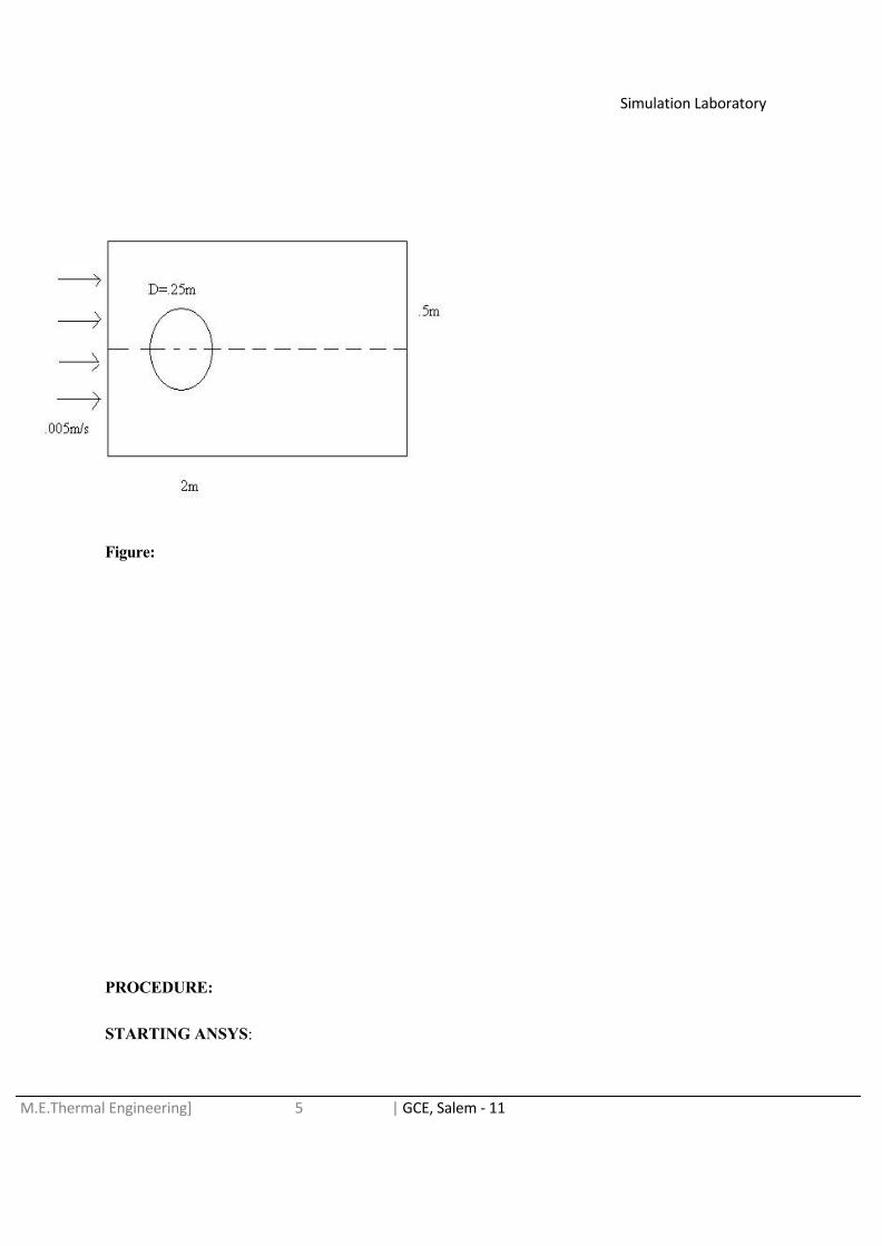
Problem Description:
Dimensions:
1) The cylinder is .25m in diameter.
2) Because of symmetry, the problem is simplifies so that half of the cylinder is
computed. The results are assumed to be the same on the other side of the x axis
(axis of symmetry).
3) The flow area is 2m by 0.5m. This arbitrary size serves to set up the boundary
conditions of flow over a cylinder.
4) The velocity of the air at infinite distance from the plate is 5 mm/s (.005m/s)
Simulation Laboratory
M.E.Thermal Engineering] 5 | GCE, Salem - 11
Figure:
PROCEDURE:
STARTING ANSYS:

Simulation Laboratory
M.E.Thermal Engineering] 5 | GCE, Salem - 11
Click on ANSYS 10.1 in the programs menu
MODELLING THE STRUCTURE:
preprocessor > Modeling >Create > Areas > Rectangle > By 2 corners.
The width is 2 and the height is .5. Starting position is at (0,0).
To create the circle
preprocessor > Modeling > Create > Areas >Circle > Solid Circle. The radius is .125 and the center is
at (0.5,0)
To subtract the circular area from the rectangle click
Preprocessor > Modeling >Operate > Booleans > Subtract > Areas.
Select the rectangle and click OK.
Next select the circle and circle OK. You will be left with this area.
ELEMENT PROPERTIES
SELECTING ELEMENT TYPE:
Preprocessor > Element Type > Add /Edit/Delete… >Flotran CFD>2D Flotran 141
MESHING
DIVIDING THE CHANNEL INTO ELEMENTS:
Preprocessor > Meshing >Size cntrls > Manual size > Lines > Picked Lines.
In the window that comes up type .02 in the `Element edge length` box. Now go to
Pre processor > Meshing > Mesh >Areas > Free.
Click the area and OK.
Simulation Laboratory
M.E.Thermal Engineering] 5 | GCE, Salem - 11
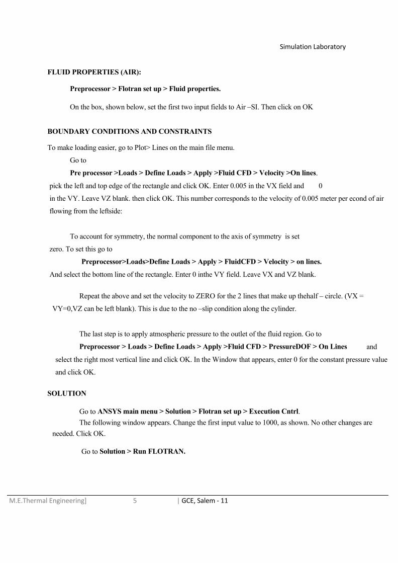
FLUID PROPERTIES (AIR):
Preprocessor > Flotran set up > Fluid properties.
On the box, shown below, set the first two input fields to Air –SI. Then click on OK
BOUNDARY CONDITIONS AND CONSTRAINTS
To make loading easier, go to Plot> Lines on the main file menu.
Go to
Pre processor >Loads > Define Loads > Apply >Fluid CFD > Velocity >On lines.
pick the left and top edge of the rectangle and click OK. Enter 0.005 in the VX field and 0
in the VY. Leave VZ blank. then click OK. This number corresponds to the velocity of 0.005 meter per econd of air
flowing from the leftside:
To account for symmetry, the normal component to the axis of symmetry is set
zero. To set this go to
Preprocessor>Loads>Define Loads > Apply > FluidCFD > Velocity > on lines.
And select the bottom line of the rectangle. Enter 0 inthe VY field. Leave VX and VZ blank.
Repeat the above and set the velocity to ZERO for the 2 lines that make up thehalf – circle. (VX =
VY=0,VZ can be left blank). This is due to the no –slip condition along the cylinder.
The last step is to apply atmospheric pressure to the outlet of the fluid region. Go to
Preprocessor > Loads > Define Loads > Apply >Fluid CFD > PressureDOF > On Lines and
select the right most vertical line and click OK. In the Window that appears, enter 0 for the constant pressure value
and click OK.
SOLUTION
Go to ANSYS main menu > Solution > Flotran set up > Execution Cntrl. The following window appears. Change the first input value to 1000, as shown. No other changes are
needed. Click OK.
Go to Solution > Run FLOTRAN.

Simulation Laboratory
M.E.Thermal Engineering] 5 | GCE, Salem - 11
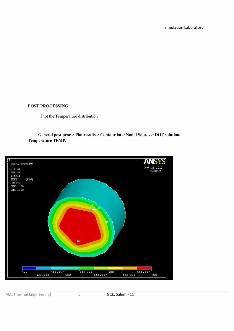
POST PROCESSING
1) Plotting the velocity distribution.
2) Go to General post proc > Read Results > Last set.
3) Then go to General Postproc > Plot Results > Contour plot > Nodal solution
select VSUM and click OK

Simulation Laboratory
M.E.Thermal Engineering] 5 | GCE, Salem - 11
TEMPERATURE DISTRIBUTION

Simulation Laboratory
M.E.Thermal Engineering] 5 | GCE, Salem - 11
VECTOR PLOT:
NOW GO TO General Post proc > Plot Results > vector Plot > Predefined and
select velocity. The vector plot looks like this.

Simulation Laboratory
M.E.Thermal Engineering] 5 | GCE, Salem - 11
VECTOR PLOT
RESULTS:
Thus the velocity distribution of a flow of air over an infinite cylinder is computed andPlotted.

Simulation Laboratory
M.E.Thermal Engineering] 5 | GCE, Salem - 11
Ex.No : 10STEADY STATE RADIATION IN SOLID CYLINDER
Date:
Aim:
To find the Temperature Distribution of the given solid cylinder by using ANSYS 10.1
Problem Description:
1. Radius of the solid is 1m.2. Height of the solid is 1m.
Boundary conditions:
1. Top side is maintained at 700°C & emissivity 0.82. Bottom side is maintained at 500°C & emissivity 0.43. Circumference is maintained at 400°C & emissivity 1(Black body)
Figure:
T=700°C & ε=0.8
T=500°C T=500°C
T=500°C & ε=0.4
PROCEDURE:

Simulation Laboratory
M.E.Thermal Engineering] 5 | GCE, Salem - 11
STARTING ANSYS:
Click on ANSYS 10.1 in the programs menu
MODELLING THE STRUCTURE:
1. Go to the ANSYS main menu2. Create geometry.
Pre-processor >Modelling >create>Volume>Cylinder>Solid cylinder>X=0,Y=0.Radius =1, Height =1
ELEMENT PROPERTIES
SELECTING ELEMENT TYPE:
Define the type of element
Pre-processor >element Type >Add //edit/Delete...>click `Add` >select Thermal masssolid, 20 node 90.
Element material properties
Pre processor > Material props> Material Modes > Thermal > conductivity>Isotropic > KXX =10 ( Thermal conductivity)
MESHING
DIVIDING THE CHANNEL INTO ELEMENTS:
Mesh Size
Preprocessor> Meshing > size cntrls > Manual size > Areas > All Areas > 0.05 Mesh
Pre processor > Meshing > Mesh > Volume > Free > Pick All

Simulation Laboratory
M.E.Thermal Engineering] 5 | GCE, Salem - 11
BOUNDARY CONDITIONS AND CONSTRAINTS
Define Analysis Type
Solution > Analysis Type > New Analysis > steady state
Apply Constraints
Solution > Define Loads > Apply>Thermal > Temperature > On Area
Apply Temperature as per the figure
Solution > Define Loads > Apply>Thermal > Radiation > On Area
Apply Emissivity as per the figure and enclosure no is 1 for all area.
Preprocessor > Radiation opts > solution opt
Fill the window in as shown to constrain the side to a Stephen Boltze man constant of 5.67e-8.7 And enclosure no is 1.
Main menu > Radiation Opt > Matrix method > other settings
Fill the window in as shown to constrain the side to a Stephen Boltze man constant of 5.67e-8.7 And type of geometry is 2D.
SOLUTION
Solve the system
Solution > solve > current LS > OK
Simulation Laboratory
M.E.Thermal Engineering] 5 | GCE, Salem - 11
POST PROCESSING
Plot the Temperature distribution
General post proc > Plot results > Contour lot > Nodal Solu… > DOF solution,Temperature TEMP.

Simulation Laboratory
M.E.Thermal Engineering] 5 | GCE, Salem - 11
TEMPERATURE DISTRIBUTION
RESULTS:
Thus the temperature distribution of the given solid is determined.
Ex.No : 11COMBINED STEADY STATE CONDUCTION AND CONVECTION IN FIN
Date:
Aim:

Simulation Laboratory
M.E.Thermal Engineering] 5 | GCE, Salem - 11
To find the temperature distribution of the given solid by using ANSYS 10.1
Problem Description:
1) Length of the fin is 1 m.2) Height of the fin is 0.5m3) Width of the fin is 5 m
Boundary condition:
1) Wall temperature is 200 C.2) Ambient air is 40 C.3) Convection Co-efficient of the wall is 50 W/m2 C4) Thermal conductivity 200 W/m C
Figure:

Simulation Laboratory
M.E.Thermal Engineering] 5 | GCE, Salem - 11
PROCEDURE:
STARTING ANSYS:
Click on ANSYS 10.1 in the programs menu
MODELLING THE STRUCTURE:
1) Go to the ANSYS Main Menu2) Create geometry
Pre-processor > Modelling > create > Volume > Block > By 2 corner & Z > Length=1, Height=0.5 , Depth = 5.
ELEMENT PROPEERTIES
SELECTING ELEMENT TYPE:
Define the Type of element
Preprocessor > Element type > Add/Edit/Delete...> click `Add` > select ThermalMass Solid, 20 node 90.
Material properties
Preprocessor > Material Props > Material models > Thermal Conductivity >Isotropic > kxx =200 (Thermal conductivity)
MESHING
DIVIDING THE SHANNEL INTO ELEMENTS:
Mesh size
Pre-processor > Meshing > Size cntrls > Manual size > Areas > All Areas > 0.05
Mesh
Pre processor > Meshing > Mesh > volume > Free > Pick All
Simulation Laboratory
M.E.Thermal Engineering] 5 | GCE, Salem - 11
BOUNDARY CONDITIONS AND CONSTRAINTS
Analysis Type
Solution > Analysis Type > New Analysis > steady state
Constrints
Solution > Define Loads > Apply
Thermal > Temperature > On Area
Apply temperature as per the figure
Solution > Define Loads > Apply
Thermal > Convection > On areas
Apply film coefficient of 50 and bulk temperature of 40 in the remaining sides’
SOLUTION
Solve the system
Solution > solve > Current LS > ok
SOLVE

Simulation Laboratory
M.E.Thermal Engineering] 5 | GCE, Salem - 11
POST PROCESSING
Plot the temperature distribution
General postproc > Plot Results > Contour plot > Nodal Solu… > DOF solution,Temperature TEMP

Simulation Laboratory
M.E.Thermal Engineering] 5 | GCE, Salem - 11

Simulation Laboratory
M.E.Thermal Engineering] 5 | GCE, Salem - 11
TEMPERATURE DISTRIBUTION
VECTOR PLOT:
Now go to General PostProc > Plot Resuots > Vector Plot > Predefined and selectvelocity.
Simulation Laboratory
M.E.Thermal Engineering] 5 | GCE, Salem - 11
RESULTS:
Thus the temperature distribution and thermal flux of the given fin is determined.
Ex.No : 12STEADY STATE CONVECTION IN COMPOSITE HOLLOW CYLINDER
Date:
Aim:
To find the temperature distribution of the given composite hollow cylinder by using ANSYS 10.1
Simulation Laboratory
M.E.Thermal Engineering] 5 | GCE, Salem - 11
Problem Description:
1. Inner diameter of the cylinder 0.025m2. Outer diameter of the cylinder 0.038m3. Inner diameter of the cylinder (insulator) 0.038m4. Outer diameter of the cylinder (insulator) 0.058m5. Depth 2m
Boundary condition:
6. Hot gas flow inside the cylinder 330 C & h=400 W/m2 C7. Outer surface of the insulator is at 30C & h=60 W/m2 C
Figure:
PROCEDURE:
STARTING ANSYS:
Simulation Laboratory
M.E.Thermal Engineering] 5 | GCE, Salem - 11
Click on ANSYS 10.1 in the programs menu
MODELLING THE STRUCTURE:
Go to the ANSYS Main Menu>Create geometry
Pre-processor >Modelling >create>Volume>Cylinder>Hollow cylinder> Rad1 =0.025, Rad2 =0.038,Depth=2
Pre-processor >Modelling >create>Volume>Cylinder>Hollow cylinder> Rad1 =0.038, Rad2 =0.058, Depth=2
Pre-processor >Modelling >operate>booleans >glue>areas
ELEMENT PROPEERTIES
SELECTING ELEMENT TYPE:
Define the Type of element
Preprocessor > Element type > Add/Edit/Delete...> click `Add` > select ThermalMaterial properties
Preprocessor>Material Props>Materialmodels1>Thermal>Conductivity>Isotropic >kxx =15
Preprocessor>Material Props>Materialmodels2>Thermal>Conductivity>Isotropic >kxx =0.2(Thermal conductivity)
MESHING
DIVIDING THE SHANNEL INTO ELEMENTS:
Mesh size
Pre-processor > Meshing > Size cntrls > Manual size > Areas > All Areas > 0.001
Mesh
Pre processor > Meshing > Mesh > Volume> Free > Pick All
BOUNDARY CONDITIONS AND CONSTRAINTS
Analysis Type

Simulation Laboratory
M.E.Thermal Engineering] 5 | GCE, Salem - 11
Solution > Analysis Type > New Analysis > steady state
Constraints
Solution > Define Loads > Apply>Thermal > Convection > on areas
Apply as per the diagram (Bulk Temperature = 330, film coefficient =400)
For Insulator
Solution > Define Loads > Apply>Thermal > Convection > On areas Apply as per the diagram (Bulk Temperature = 30, film coefficient =60)
SOLUTION
Solve the system
Solution > solve > Current LS> Ok
SOLVE
POST PROCESSING
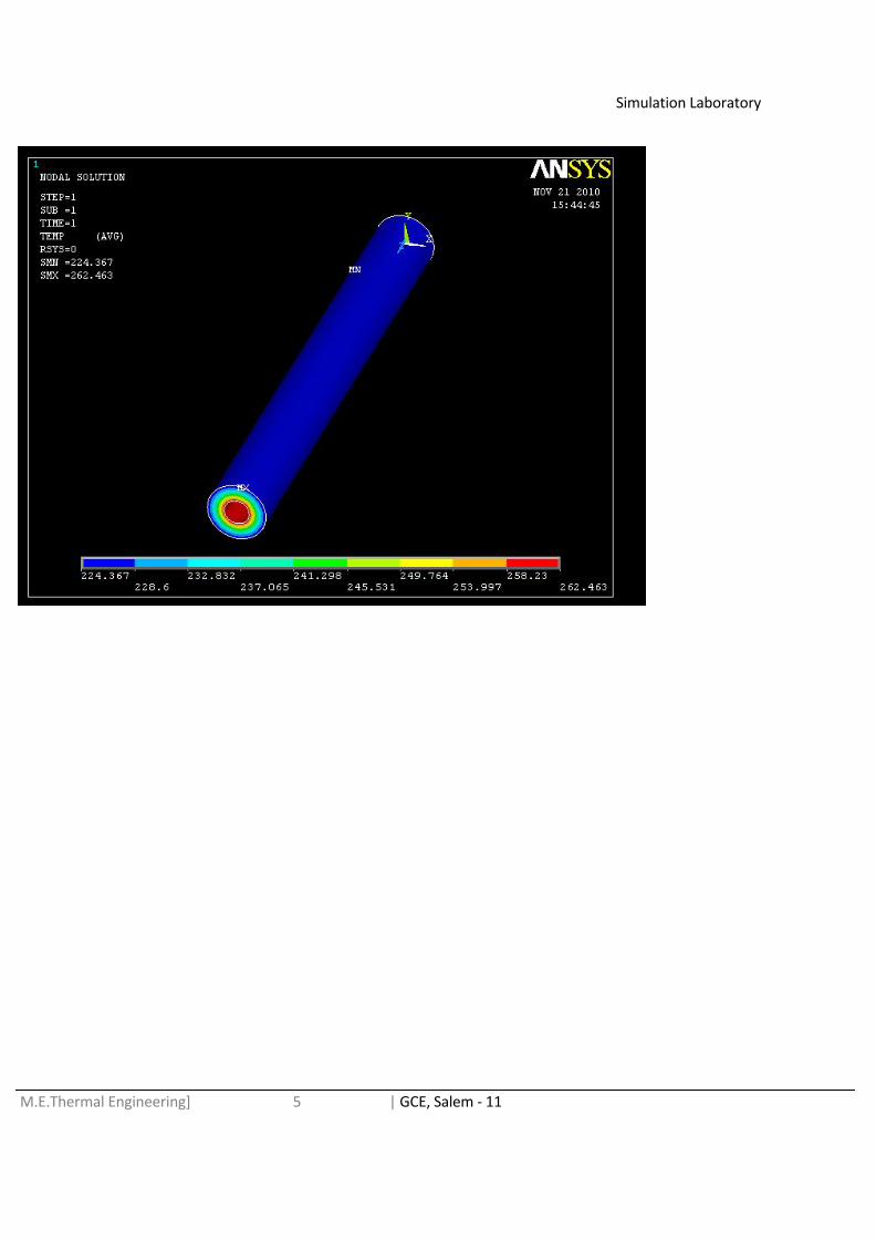
Plot the temperature distribution
General postproc > Plot Results > contour plot > Nodal Solu… > DOF solution,Temperature TEMP
Simulation Laboratory
M.E.Thermal Engineering] 5 | GCE, Salem - 11

Simulation Laboratory
M.E.Thermal Engineering] 5 | GCE, Salem - 11
TEMPERATURE DISTRIBUTION
POST PROCESSING
Plot the temperature distribution
General postproc > Plot Results > contour plot > Nodal Solu… > DOF solution,Temperature TEMP
Simulation Laboratory
M.E.Thermal Engineering] 5 | GCE, Salem - 11
TEMPERATURE DISTRIBUTION
VECTOR PLOT:
Plot the temperature distribution
Now go to General PostProc > Plot Results > Vector Plot > Predefined and Thermal Flux
Simulation Laboratory
M.E.Thermal Engineering] 5 | GCE, Salem - 11

Simulation Laboratory
M.E.Thermal Engineering] 5 | GCE, Salem - 11
RESULTS:
Thus the temperature distribution of the given composite hollow cylinder is determined.

Simulation Laboratory
M.E.Thermal Engineering] 5 | GCE, Salem - 11
Ex.No : 13COMBINED CONDUCTION AND CONVECTION IN TRIANGULAR FIN
Date:
Aim:
To find the Temperature distribution of the given triangular fin by using ANSYS 10.1
Problem Description:
1. Length of the fin is 0.04 m.2. Side of the fin is 0.005m.3. Wall temperature is 400 C4. Convection Co-efficient of the wall is 90 W/m2C5. Bulk Temperature 50 C
Figure
PROCEDURE;

Simulation Laboratory
M.E.Thermal Engineering] 5 | GCE, Salem - 11
STARTING ANSYS:
Click on ANSYS 10.1 in the program menu.
MODELLING THE STRUCTURE:
1) Go to the ANSYS main menu.2) Create geometry.
Preprocessor > Modeling > create > Volume> Prism > By Side Lengths> Z=0.04, Side=0.005
ELEMENT PROPERTIES
SELECTING ELEMENT TYPE:
Define the type of element
Preprocessor > Element Type > Add/Edit/Delete >click `Add` > select
Thermal Mass Solid, 20 node90
Element material properties
Preprocessor> Material props > Material Models > Thermal conductivity>Isotropic > KXX = 54 (Thermal conductivity)
MESHING
DIVIDING THE CHANNEL INTO ELEMENTS:
Mesh Size
Preprocessor > Meshing > size cntrls > Manual size > Areas > All areas > 0.05
Mesh
Simulation Laboratory
M.E.Thermal Engineering] 5 | GCE, Salem - 11
Preprocessor > Meshing > Mesh > Volume > Free > Pick all
BOUNDARY CONDITIONS AND CONSTRAINTS
Define Analysis Type
Solution > Analysis Type > New Analysis > steay state
Apply Constraints
Solution > Define Loads > Apply Thermal > Temperature > Online Areas
Apply as per the drawing
Solution > Define Loads > Apply Thermal > Convection> Online Areas
Apply as per the figure (film coefficient of 90 and bulk temperature of 50.)
SOLUTION
Solve the system
Solution > solve > current LS>Ok
SOLVE
POST PROCESSING

Simulation Laboratory
M.E.Thermal Engineering] 5 | GCE, Salem - 11
Plot the temperature distribution
General postproc > Plot results > Contour Plot > Nodal Solu…> DOF solution ,Temperature TEMP

Simulation Laboratory
M.E.Thermal Engineering] 5 | GCE, Salem - 11
TEMPERATURE DISTRIBUTION

Simulation Laboratory
M.E.Thermal Engineering] 5 | GCE, Salem - 11
VECTOR PLOT:
Plot the temperature distribution
General PostProc > Plot Results > Vector Plot > Predefined and Thermal Flux

Simulation Laboratory
M.E.Thermal Engineering] 5 | GCE, Salem - 11
RESULT:
Thus the temperature distribution and thermal flux of the given fin is determined.

Simulation Laboratory
M.E.Thermal Engineering] 5 | GCE, Salem - 11
Ex.No : 14RADIATION HEAT TRANSFER IN TRIANGULAR FIN
Date:
Aim:
To find the Temperature distribution of the given triangular strip by using ANSYS 10.1
Problem Description:
1. Radius of the strip is 1 m.2. Angle of the strip is 60.3. Wall temperature at the sides are 900 C and 400 C respectively4. Emissivities of the sides are 0.8 for both sides.5. Heat transfer at the bottom side is zero6. K=30 W/m C
Figure

Simulation Laboratory
M.E.Thermal Engineering] 5 | GCE, Salem - 11
PROCEDURE;STARTING ANSYS:
Click on ANSYS 10.1 in the program menu.
MODELLING THE STRUCTURE:
1) Go to the ANSYS main menu.2) Create geometry.
Preprocessor > Modeling > create > Area> Polygon >Triangle> X=0,Y=0, Radius=1,Theta=60Preprocessor > Modeling > create > Area> Circle >Solid circle> X=0,Y=0, Radius=0.5
ELEMENT PROPERTIES
SELECTING ELEMENT TYPE:
Define the type of element
Preprocessor > Element Type > Add/Edit/Delete >click `Add` > select
Thermal Mass Solid, Quad node55
Element material properties
Preprocessor> Material props > Material Models > Thermal conductivity>Isotropic > KXX = 30 (Thermal conductivity)
MESHING
DIVIDING THE CHANNEL INTO ELEMENTS:
Mesh Size
Preprocessor > Meshing > size cntrls > Manual size > Areas > All areas > 0.05
Mesh

Simulation Laboratory
M.E.Thermal Engineering] 5 | GCE, Salem - 11
Preprocessor > Meshing > Mesh > Areas > Free > Pick all
Simulation Laboratory
M.E.Thermal Engineering] 5 | GCE, Salem - 11
BOUNDARY CONDITIONS AND CONSTRAINTS
Define Analysis Type
Solution > Analysis Type > New Analysis > steay state
Apply Constraints
Solution > Define Loads > Apply >Thermal > Temperature > Online
Apply as per the drawing
Solution > Define Loads > Apply >Thermal > radiation> Online
Apply as per the figure (Emissivity)
SOLUTION
Solve the system
Solution > solve > current LS>Ok
SOLVE
Simulation Laboratory
M.E.Thermal Engineering] 5 | GCE, Salem - 11
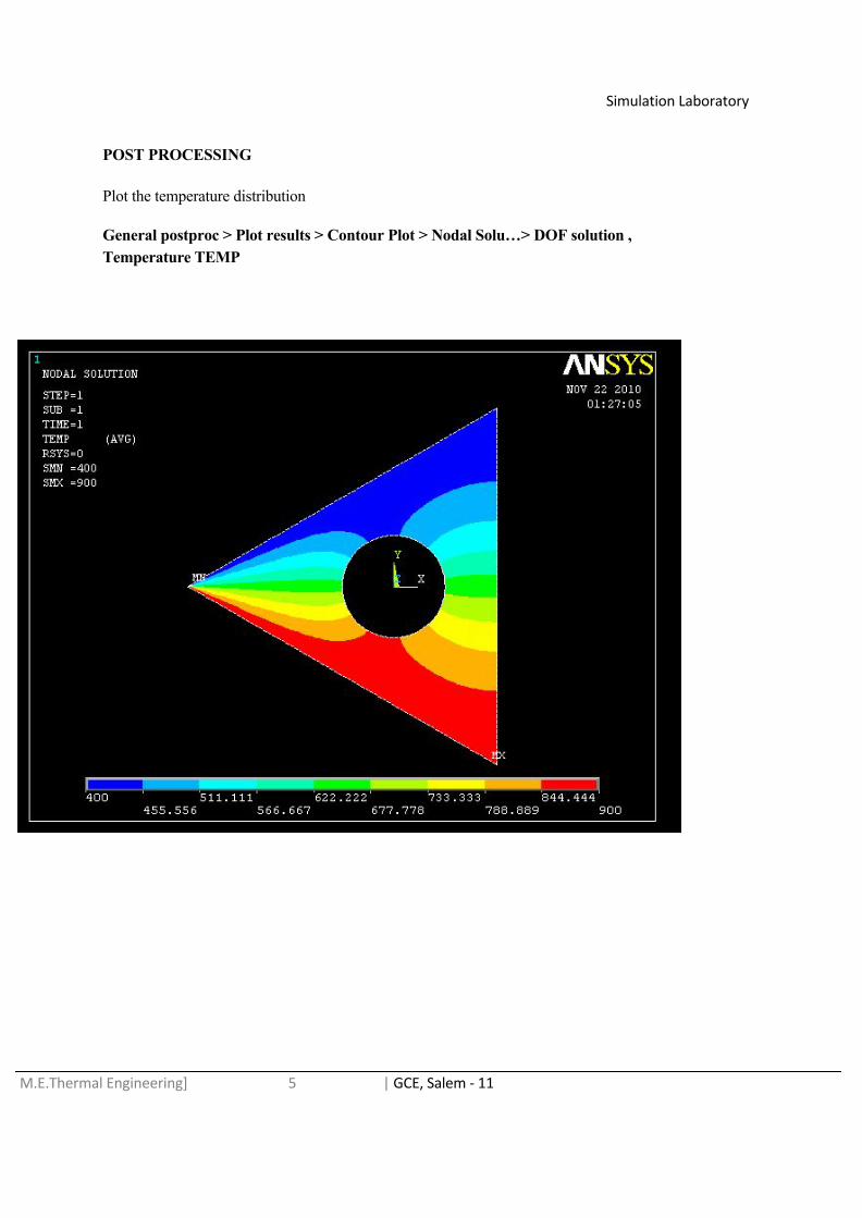
POST PROCESSING
Plot the temperature distribution
General postproc > Plot results > Contour Plot > Nodal Solu…> DOF solution ,Temperature TEMP

Simulation Laboratory
M.E.Thermal Engineering] 5 | GCE, Salem - 11
TEMPERATURE DISTRIBUTION
VECTOR PLOT:
Plot the temperature distribution
General PostProc > Plot Results > Vector Plot > Predefined and Thermal Flux

Simulation Laboratory
M.E.Thermal Engineering] 5 | GCE, Salem - 11
Simulation Laboratory
M.E.Thermal Engineering] 5 | GCE, Salem - 11
RESULT:
Thus the temperature distribution and thermal flux of the given fin is determined.
Related Documents