Simulation and Validation of Turbulent Pipe Flowsuser.engineering.uiowa.edu/~fluids/Posting/Home/CFD/Introductory/Lab 1... · Simulation and Validation of Turbulent Pipe Flows 57:020

Simulation and Validation of Turbulent Pipe Flows

57:020 Mechanics of Fluids and Transport Processes CFD LAB 1

By Timur Dogan, Michael Conger, Maysam Mousaviraad, Tao Xing and Fred Stern IIHR-Hydroscience & Engineering

The University of Iowa C. Maxwell Stanley Hydraulics Laboratory

Iowa City, IA 52242-1585 1. Purpose The Purpose of CFD Lab 1 is to teach students how to use ANSYS, practice more options in each step of CFD Process, and relate simulation results to EFD and AFD concepts. Students will simulate turbulent pipe flow following the “CFD process” by an interactive step-by-step approach. The flow conditions will be the same as they used in EFD Lab2. Students will have “hands-on” experiences using ANSYS to compute axial velocity profile, centerline velocity, centerline pressure, and wall shear stress. Students will compare simulation results with their own EFD data, analyze the differences and possible numerical/experimental errors, and present results in a CFD Lab report.

Flow chart for “CFD Process” for pipe flow

Geometry Physics Mesh Solution Results

Pipe (ANSYS Design Modeler)

Structure (ANSYS Mesh)

Non-uniform (ANSYS Mesh)

Uniform (ANSYS Mesh)

General (ANSYS Fluent - Setup) Model (ANSYS Fluent - Setup)

Boundary Conditions

(ANSYS Fluent -Setup)

Reference Values (ANSYS Fluent -

Setup)

Turbulent

Solution Methods

(ANSYS Fluent - Solution)

Monitors (ANSYS Fluent -

Solution)

Solution Initialization

(ANSYS Fluent -Solution)

Plots (ANSYS Fluent- Results)

Graphics and Animations

(ANSYS Fluent- Results)

1

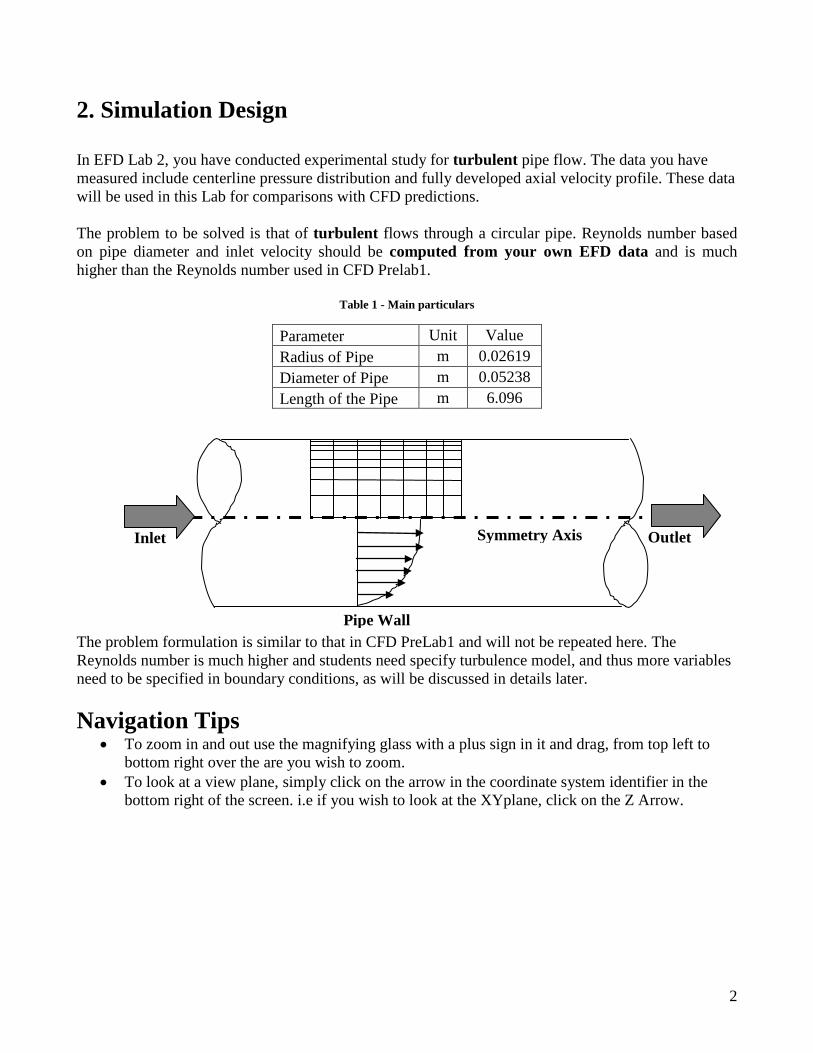
2. Simulation Design In EFD Lab 2, you have conducted experimental study for turbulent pipe flow. The data you have measured include centerline pressure distribution and fully developed axial velocity profile. These data will be used in this Lab for comparisons with CFD predictions. The problem to be solved is that of turbulent flows through a circular pipe. Reynolds number based on pipe diameter and inlet velocity should be computed from your own EFD data and is much higher than the Reynolds number used in CFD Prelab1.

Table 1 - Main particulars

Parameter Unit Value Radius of Pipe m 0.02619 Diameter of Pipe m 0.05238 Length of the Pipe m 6.096

The problem formulation is similar to that in CFD PreLab1 and will not be repeated here. The Reynolds number is much higher and students need specify turbulence model, and thus more variables need to be specified in boundary conditions, as will be discussed in details later. Navigation Tips

• To zoom in and out use the magnifying glass with a plus sign in it and drag, from top left to bottom right over the are you wish to zoom.

• To look at a view plane, simply click on the arrow in the coordinate system identifier in the bottom right of the screen. i.e if you wish to look at the XYplane, click on the Z Arrow.

Outlet Inlet Symmetry Axis

Pipe Wall

2

3. Open ANSYS Workbench 3.1. Start > All Programs > ANSYS 14.5 > Workbench 14.5

3.2. From the ANSYS Workbench home screen (Project Schematic), drag and drop the Fluid Flow (Fluent) component from the Toolbox on the left side of the screen into the Project Schematic. Name each component as per below.

3.3. Create connection as per below by dragging and dropping each component to the corresponding component.

3

3.4. Create a Folder on the H: Drive called CFD Lab 1. 3.5. Save the project file by clicking File > Save As… 3.6. Save the project onto the H: Drive in the folder you just created and name it CFD Lab 1

Turbulent Flow.

4. Geometry 4.1. Right click on Geometry and from the drop down menu select New Geometry…

4

4.2. Select Meter for unit and click OK.

4.3. Select the XYPlane under the Tree Outline and click New Sketch button.

4.4. Right click XYPlane and select Look at.

5

4.5. Select Sketching > Rectangle. Create a rectangle geometry as per below.

4.6. Select Dimensions > General. Click on top edge then click anywhere. Repeat the same thing for one of the vertical edges. You should have a similar figure as per below.

4.7. Click on H1under Details View and change it to 6.096m. Click on V2 and change it to 0.02619m.

NOTE: The actual length of the pipe is 30 feet (9.144m), However, in CFD simulation, we need to specify “outlet pressure”, and we don’t have a pressure transducer at the pipe outlet. So we choose the outlet of the pipe we will simulate to be the location of the last pressure transducer, which is 6.096 meters from the pipe inlet.

6

4.8. Concept > Surface From Sketches and select the sketch and hit Apply.

4.9. Click Generate. This will create a surface.

7

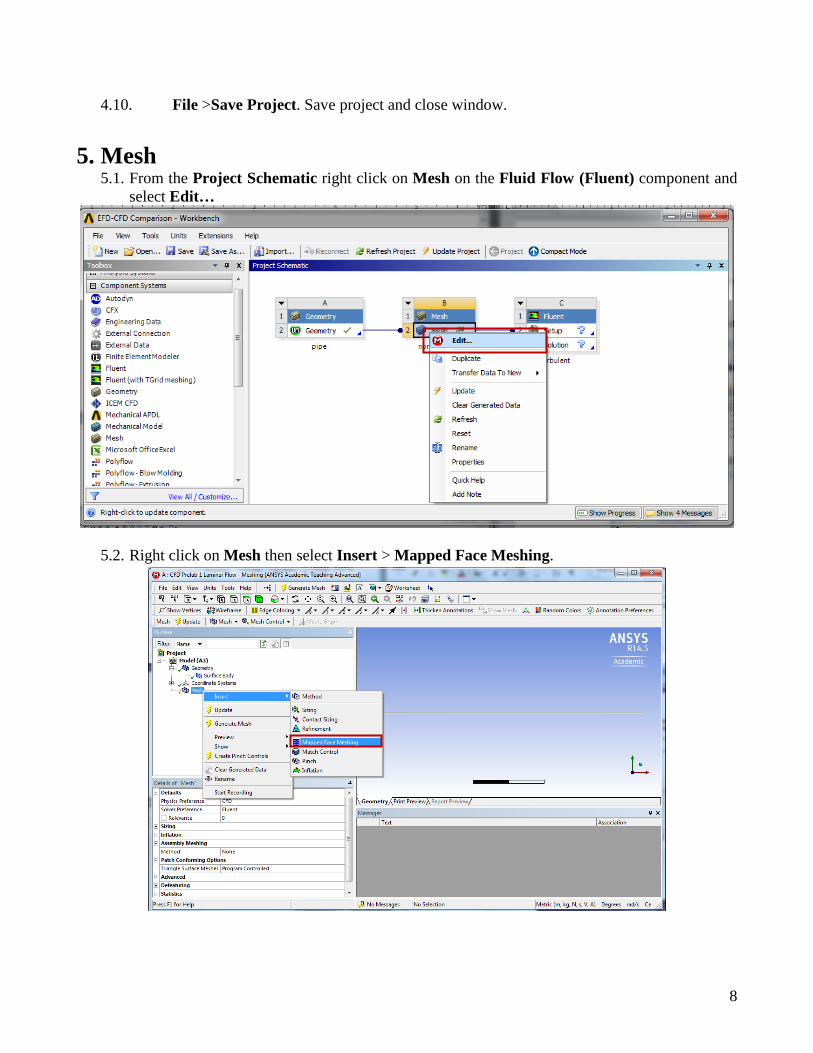
4.10. File >Save Project. Save project and close window. 5. Mesh

5.1. From the Project Schematic right click on Mesh on the Fluid Flow (Fluent) component and select Edit…

5.2. Right click on Mesh then select Insert > Mapped Face Meshing.

8

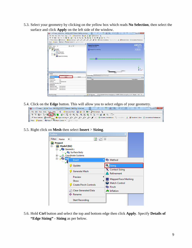
5.3. Select your geometry by clicking on the yellow box which reads No Selection, then select the surface and click Apply on the left side of the window.

5.4. Click on the Edge button. This will allow you to select edges of your geometry.

5.5. Right click on Mesh then select Insert > Sizing.

5.6. Hold Ctrl button and select the top and bottom edge then click Apply. Specify Details of “Edge Sizing” - Sizing as per below.

9

5.7. Repeat step 5.5. 5.8. Select the left edge then click Apply and change the parameters as per below.

5.9. Repeat Step 5.5. 5.10. Select the right edge then click Apply and change the parameters as per below.

5.11. Click on Generate Mesh button and then select Mesh under Outline. The mesh should look like the mesh below.

10

5.12. Change the edge names by selecting the edge, then right clicking on the edge and selecting Create Named Selection from the drop down menu. Name left, right, bottom and top edges as inlet, outlet, axis and wall respectively then click OK. Your outline should look same as the figure below.

11

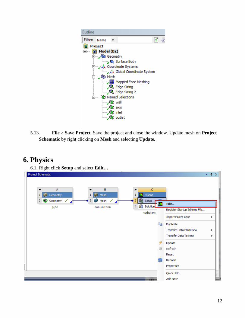
5.13. File > Save Project. Save the project and close the window. Update mesh on Project

Schematic by right clicking on Mesh and selecting Update.

6. Physics 6.1. Right click Setup and select Edit…

12

6.2. Check Double Precision.

6.3. Solution Setup > General > Check. (Note: If you get and error message you may have made a mistake while creating you mesh)

13

6.4. Solution Setup > General > Solver. Choose options shown below.(Note: using axisymmetric sets the derivative du/dy at the axis to zero. This is considered a boundary condition on the axis.)

6.5. Solution Setup > Models > Viscous–Laminar > Edit… Select k-epsilon (2 eqn) and click OK.

14

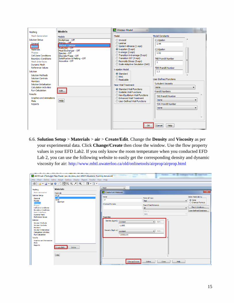
6.6. Solution Setup > Materials > air > Create/Edit. Change the Density and Viscosity as per your experimental data. Click Change/Create then close the window. Use the flow property values in your EFD Lab2. If you only know the room temperature when you conducted EFD Lab 2, you can use the following website to easily get the corresponding density and dynamic viscosity for air: http://www.mhtl.uwaterloo.ca/old/onlinetools/airprop/airprop.html

15

If the room temperature is 24°, the density and viscosity are the values shown in the above panel. NOTE: viscosity used in ANSYS is the dynamic viscosity ( kg m s⋅ ), NOT kinematic viscosity ( 2m s )

6.7. Solution Setup > Cell Zone Conditions > Zone > surface_body. Change type to fluid and

click OK. Select Material Name as air and click OK.

16

6.8. Solution Setup > Boundary Conditions > inlet > Edit… Change parameters as per your experimental data and click OK. You must calculate the inlet velocity u, which is uniform, based on the flow rate Q (m3/s) you computed in EFD Lab2, and cross section area of the pipe

2 4Dπ , i.e. 24u Q Dπ=

17

6.9. Solution Setup > Boundary Conditions > outlet > Edit… Change parameters as per

experimental data and click OK. You need to transform the four pressure tap pressure values from “feet water” to “Pascal” and input pressure tap #4 value as the “outlet pressure”. For example, if the pressure tap #4 has value of 0.2502 feet water, you need input 747 Pascal.

18

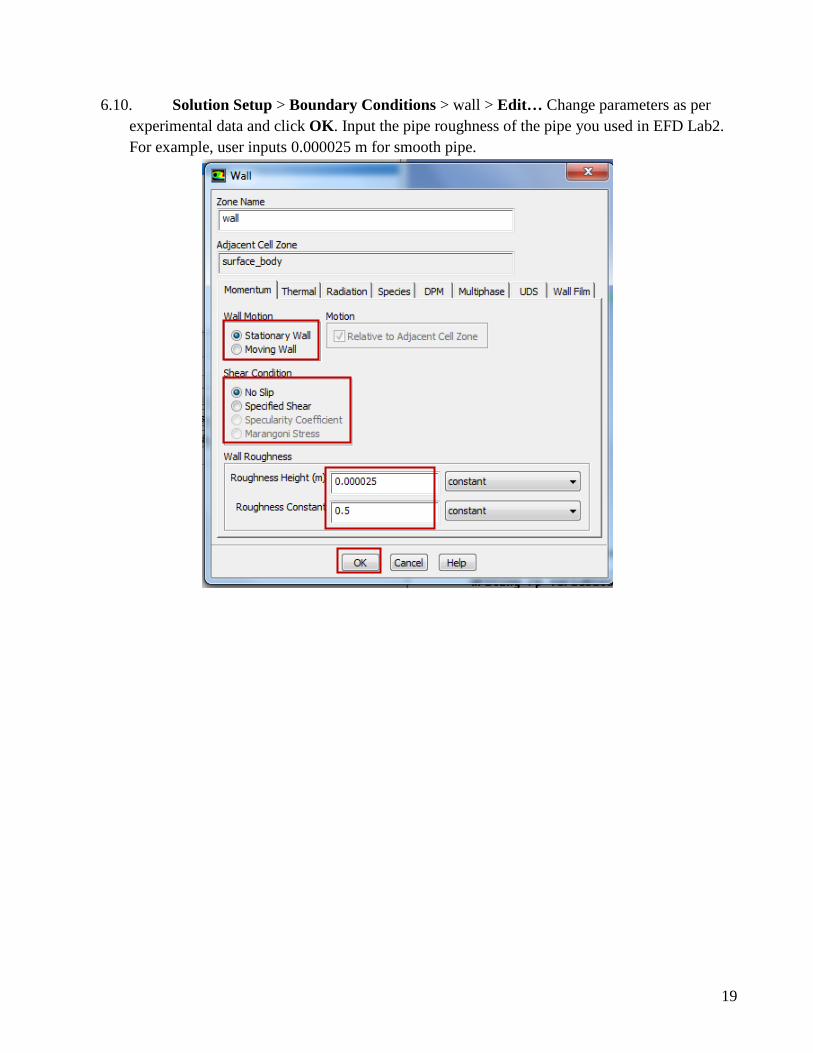
6.10. Solution Setup > Boundary Conditions > wall > Edit… Change parameters as per experimental data and click OK. Input the pipe roughness of the pipe you used in EFD Lab2. For example, user inputs 0.000025 m for smooth pipe.

19

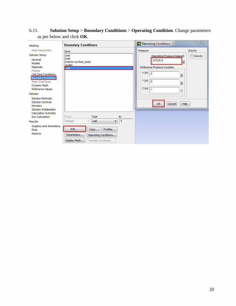
6.11. Solution Setup > Boundary Conditions > Operating Condition. Change parameters as per below and click OK.

20

6.12. Solution Setup > Reference Values. Change parameters as per experimental data. Parameters in blue are constant and should be entered as seen below. Parameters in red are from experimental data.

21

7. Solution 7.1. Solution > Solution Methods. Change parameters as per below.

7.2. Solution > Monitors > Residuals –Print, Plot > Edit… Change convergence criterion to 1e-06 for all five equations as per below and click OK.

22

7.3. Solution > Solution Initialization. Change parameters as per experimental data and click Initialize. Parameters in blue are constant and should be entered as seen below. Parameters in red are from experimental data.

7.4. Solution > Run calculation. Change Number of Iterations to 1000 and click Calculate.

23

7.5. Once the solution converges, click OK. (The residuals should be comparable to the ones

below.)

7.6. File > Save Project. Save the project.

8. Results 8.1. Displaying Mesh

Display > Mesh. Select all Surfaces you wish to be visible and select Display then click Close.

24

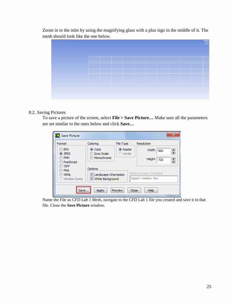
Zoom in to the inlet by using the magnifying glass with a plus sign in the middle of it. The mesh should look like the one below.

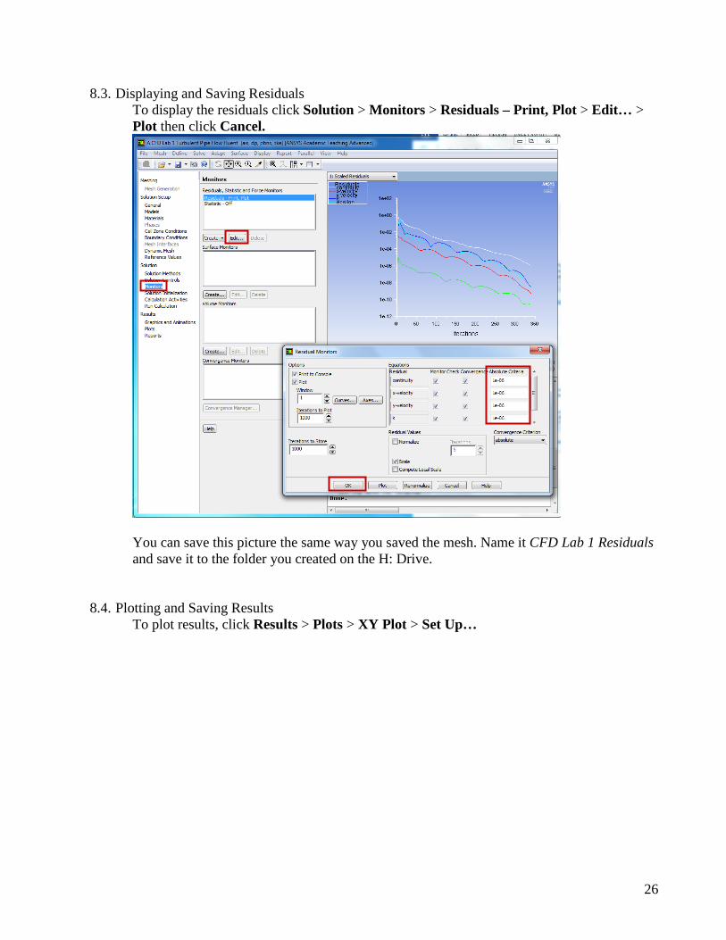
8.2. Saving Pictures To save a picture of the screen, select File > Save Picture… Make sure all the parameters are set similar to the ones below and click Save…

Name the File as CFD Lab 1 Mesh, navigate to the CFD Lab 1 file you created and save it in that file. Close the Save Picture window.

25

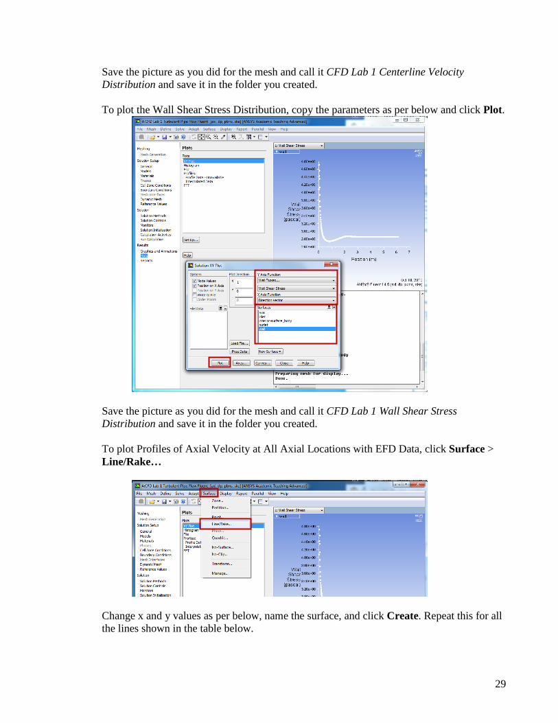
8.3. Displaying and Saving Residuals To display the residuals click Solution > Monitors > Residuals – Print, Plot > Edit… > Plot then click Cancel.

You can save this picture the same way you saved the mesh. Name it CFD Lab 1 Residuals and save it to the folder you created on the H: Drive.

8.4. Plotting and Saving Results To plot results, click Results > Plots > XY Plot > Set Up…

26

To plot the Centerline Pressure Distribution, copy the parameters as per below. Next click Load File…, select the file named pressure-EFD-turbulent-pipe.xy and click OK. Then click Plot. This .xy file can be downloaded from the class website. The plot should look similar to the one below. http://www.engineering.uiowa.edu/~fluids/

27

You can save this picture the same way you saved the mesh. Name it CFD Lab 1 Center Line Pressure with EFD and save it to the folder you created on the H: Drive.

To plot Centerline Velocity Distribution, copy the parameters as per below, select Pressure Profile from the File Data menu, make sure that it is NOT highlighted, and click Plot.

28

Save the picture as you did for the mesh and call it CFD Lab 1 Centerline Velocity Distribution and save it in the folder you created.

To plot the Wall Shear Stress Distribution, copy the parameters as per below and click Plot.

Save the picture as you did for the mesh and call it CFD Lab 1 Wall Shear Stress Distribution and save it in the folder you created.

To plot Profiles of Axial Velocity at All Axial Locations with EFD Data, click Surface > Line/Rake…

Change x and y values as per below, name the surface, and click Create. Repeat this for all the lines shown in the table below.

29

Surface Name X0 Y0 X1 Y1

x=10d 0.5238 0 0.5238 0.02619 x=20d 1.0476 0 1.0476 0.02619 x=40d 2.0952 0 2.0952 0.02619 x=60d 3.1428 0 3.1428 0.02619 x=100d 5.238 0 5.238 0.02619

When all lines are created, click Close. Next you should open the file axialvelocityEFD-turbulent-pipe.xy with a text editor and replace the velocity values with the values you recorded experimentally. Save the file. Click Load File… and select axialvelocityEFD-turbulent-pipe.xy, which is the file you just modified, and click OK. Change Parameters as per below. Make sure to select inlet as well.

30

Click Curves… > Change the Pattern to the pattern seen below and click Apply. Do this for curves 0 through 7 then click Close.

Click Plot.

31

Save the picture as you did for the mesh and call it CFD Lab 1 Axial Velocity at All Axial Locations with EFD Data and save it in the folder you created.

8.5. Plotting and Saving Graphics

Click Results > Graphics and Animations > Vectors > Set Up… To plot the velocity vectors at the region flow begin to become fully developed, copy the parameters as per below and click Display.

32

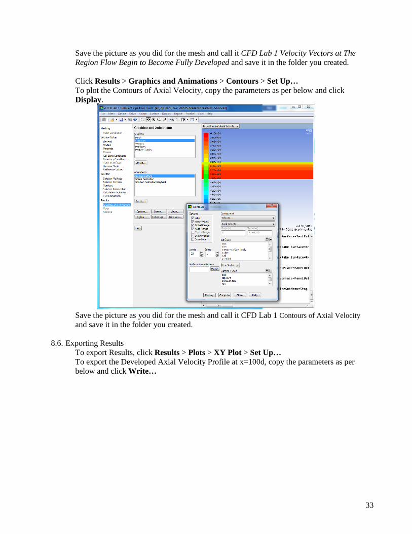
Save the picture as you did for the mesh and call it CFD Lab 1 Velocity Vectors at The Region Flow Begin to Become Fully Developed and save it in the folder you created. Click Results > Graphics and Animations > Contours > Set Up… To plot the Contours of Axial Velocity, copy the parameters as per below and click Display.

Save the picture as you did for the mesh and call it CFD Lab 1 Contours of Axial Velocity and save it in the folder you created.

8.6. Exporting Results To export Results, click Results > Plots > XY Plot > Set Up… To export the Developed Axial Velocity Profile at x=100d, copy the parameters as per below and click Write…

33

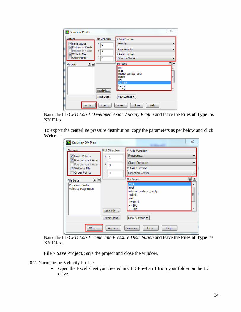
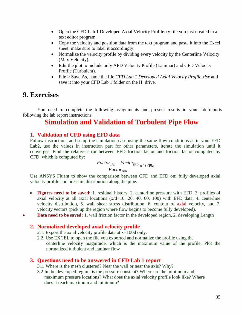
Name the file CFD Lab 1 Developed Axial Velocity Profile and leave the Files of Type: as XY Files. To export the centerline pressure distribution, copy the parameters as per below and click Write…

Name the file CFD Lab 1 Centerline Pressure Distribution and leave the Files of Type: as XY Files. File > Save Project. Save the project and close the window.

8.7. Normalizing Velocity Profile • Open the Excel sheet you created in CFD Pre-Lab 1 from your folder on the H:

drive.

34

• Open the CFD Lab 1 Developed Axial Velocity Profile.xy file you just created in a text editor program.

• Copy the velocity and position data from the text program and paste it into the Excel sheet, make sure to label it accordingly.

• Normalize the velocity profile by dividing every velocity by the Centerline Velocity (Max Velocity).

• Edit the plot to include only AFD Velocity Profile (Laminar) and CFD Velocity Profile (Turbulent).

• File > Save As, name the file CFD Lab 1 Developed Axial Velocity Profile.xlsx and save it into your CFD Lab 1 folder on the H: drive.

9. Exercises

You need to complete the following assignments and present results in your lab reports

following the lab report instructions Simulation and Validation of Turbulent Pipe Flow

1. Validation of CFD using EFD data Follow instructions and setup the simulation case using the same flow conditions as in your EFD Lab2, use the values in instruction part for other parameters, iterate the simulation until it converges. Find the relative error between EFD friction factor and friction factor computed by CFD, which is computed by:

100%CFD EFD

EFD

Factor FactorFactor

−×

Use ANSYS Fluent to show the comparison between CFD and EFD on: fully developed axial velocity profile and pressure distribution along the pipe. • Figures need to be saved: 1. residual history, 2. centerline pressure with EFD, 3. profiles of

axial velocity at all axial locations (x/d=10, 20, 40, 60, 100) with EFD data, 4. centerline velocity distribution, 5. wall shear stress distribution, 6. contour of axial velocity, and 7. velocity vectors (pick up the region where flow begins to become fully developed).

• Data need to be saved: 1. wall friction factor in the developed region, 2. developing Length 2. Normalized developed axial velocity profile

2.1. Export the axial velocity profile data at x=100d only. 2.2. Use EXCEL to open the file you exported and normalize the profile using the

centerline velocity magnitude, which is the maximum value of the profile. Plot the normalized turbulent and laminar flow

3. Questions need to be answered in CFD Lab 1 report

3.1. Where is the mesh clustered? Near the wall or near the axis? Why? 3.2 In the developed region, is the pressure constant? Where are the minimum and maximum pressure locations? What does the axial velocity profile look like? Where does it reach maximum and minimum?

35

3.3 Where is the developing region? How can you determine the length of the developing region? (hint: centerline velocity). What is the difference for axial velocity profile between “developing” region and “developed” region?

3.4. Compare the normalized axial velocity profiles for laminar and turbulent pipe flows at x=100d, discuss the difference of axial velocity gradient (du/dy) on the wall, which is larger?

3.5. What are the correct boundary conditions (velocities u, v and pressure) on the pipe wall and on the pipe centerline? 3.6. Summarize your findings and use the knowledge you learned from classroom lectures, textbooks and ANSYS figures to answer questions.

36