SIMULATION AND TESTING OF RESIN INFUSION MANUFACTURING PROCESSES FOR LARGE COMPOSITE STRUCTURES by Daniel Blair Mastbergen A thesis submitted in partial fulfillment of the requirements for the degree of Master of Science in Mechanical Engineering MONTANA STATE UNIVERSITY-BOZEMAN Bozeman, Montana JULY 2004

Welcome message from author
This document is posted to help you gain knowledge. Please leave a comment to let me know what you think about it! Share it to your friends and learn new things together.
Transcript

SIMULATION AND TESTING OF RESIN INFUSION MANUFACTURING
PROCESSES FOR LARGE COMPOSITE STRUCTURES
by
Daniel Blair Mastbergen
A thesis submitted in partial fulfillment of the requirements for the degree
of
Master of Science
in
Mechanical Engineering
MONTANA STATE UNIVERSITY-BOZEMAN Bozeman, Montana
JULY 2004

©COPYRIGHT
by
Daniel Blair Mastbergen
2004
All Rights Reserved
ii
APPROVAL
of a thesis submitted by
Daniel Blair Mastbergen This thesis has been read by each member of the thesis committee and has been found to be satisfactory regarding content, English usage, format, citations, bibliographic style, and consistency, and is ready for submission to the College of Graduate Studies. Dr. Douglas Cairns
Approved for the Department of Mechanical and Industrial Engineering Dr. Vic Cundy
Approved for the College of Graduate Studies Dr. Bruce McLeod

iii
STATEMENT OF PERMISSION TO USE
In presenting this thesis in partial fulfillment of the requirements for a master's degree at Montana State University-Bozeman, I agree that the Library shall make it avail-able to borrowers under rules of the Library. If I have indicated my intention to copyright this thesis by including a copyright notice page, copying is allowable only for scholarly purposes, consistent with "fair use" as prescribed in the U.S. Copyright Law. Requests for permission for extended quotation from or reproduction of this thesis in whole or in parts may be granted only by the copy-right holder. Daniel Mastbergen Date 7-19-04
iv
TABLE OF CONTENTS
LIST OF TABLES ............................................................................................................ vii LIST OF FIGURES ..........................................................................................................viii
ABSTRACT........................................................................................................................xi 1. INTRODUCTION .......................................................................................................... 1 2. GENERAL BACKGROUND......................................................................................... 4
Composite Materials ........................................................................................................4
Matrix Materials...........................................................................................................6 Reinforcement Materials..............................................................................................7 Fiber Volume Fraction...............................................................................................10 Porosity ......................................................................................................................11
Manufacturing Processes ...............................................................................................12 Blade Design ..................................................................................................................17
3. PROCESS MODELING BACKGROUND...................................................................20
Stokes Flow....................................................................................................................22 Injection System Modeling ............................................................................................23 Channel Flow Modeling ................................................................................................29 Fabric Flow Modeling....................................................................................................32
Darcy Flow.................................................................................................................32 Saturated vs. Unsaturated Flow .................................................................................34 Fabric Compressibility...............................................................................................38 Calculating Saturation Time ......................................................................................42
Comprehensive Model...................................................................................................44 Methodology ..............................................................................................................44 Building the Matrix....................................................................................................46 Assumptions...............................................................................................................53
4. EXPERIMENTAL PROCEDURES AND EQUIPMENT............................................55
Test Fluid .......................................................................................................................55 Injection System Tests ...................................................................................................57 Channel Flow Tests........................................................................................................58 Fabric Flow Tests...........................................................................................................60
Fabrics Tested ............................................................................................................60 Fabric Compaction Data ............................................................................................62
v
Air Permeability Tester ..........................................................................................62 Liquid Permeability Tester.....................................................................................65 Permeability Testing Procedures ............................................................................66 Capillary Pressure Tests .........................................................................................68
Comprehensive Model Tests......................................................................................69 5. EXPERIMENTAL RESULTS AND ANALYTICAL CORRELATIONS..................72
Injection System Test Results ....................................................................................72 Channel Flow Test Results.........................................................................................73 Fabric Test Results ....................................................................................................75
Fabric Compaction Data.........................................................................................75 Liquid Permeability Test Results............................................................................77 Air Permeability Test Results.................................................................................81 Capillary Test Results ............................................................................................82
Comprehensive Model Test Results ...........................................................................84
6. PARAMETRIC STUDY............................................................................................90 Channel Height ..........................................................................................................90 Injection System ........................................................................................................97 Injection Pressure ....................................................................................................100 Fabric Permeability..................................................................................................102 Fabric Thickness......................................................................................................104
7. DISCUSSION OF RESULTS..................................................................................107 Fabric Tests .............................................................................................................107 Air Permeability Testing..........................................................................................109 Comprehensive Model.............................................................................................111 Limitations of the Model..........................................................................................114 Parametric Study .....................................................................................................118
8. CONCLUSIONS AND FUTURE WORK ...............................................................121
Application to Manufacturing ..................................................................................121 Injection System / Channel Flow Modeling..............................................................123
Injection System / Channel Flow Future Work.....................................................123 Fabric Tests .............................................................................................................124
Fabric Test Future Work ......................................................................................125 Comprehensive Model.............................................................................................126
Comprehensive Model Future Work ....................................................................127

vi
REFERENCES CITED ...............................................................................................128 APPENDICES.............................................................................................................129
Appendix A – Matlab Program for Entire Process....................................................133 Appendix B – Hose System Calculations from Mathcad ..........................................144 Appendix C – Permeability Data..............................................................................147 Appendix D – Compaction Data ..............................................................................149 Appendix E – Input to Model for Experimental Correlations....................................151

vii
LIST OF TABLES
Table Page
1. Summary of manufacturing process details. .....................................................17
2. Results from hose system tests.........................................................................73
3. Results from channel flow experiments............................................................74
4. Comparison of air permeability results and liquid permeability results .............82
5. Effect of varying parameters ..........................................................................120

viii
LIST OF FIGURES
Figure Page
1. Micrograph of fibers and resin ...........................................................................6
2. Fabric roll ..........................................................................................................9
3. Unidirectional, double bias and woven roving fabrics ........................................9
4. Schematic for pressure bag molding.................................................................15
5. Pressure bag molding during stage one ............................................................16
6. Blade construction ...........................................................................................18
7. Blade cross section ..........................................................................................18
8. Injection system diagram .................................................................................27
9. Correction factor for channel aspect ratio.........................................................30
10. Illustration of dual scale flow...........................................................................37
11. Pressure gradient as flow front progresses........................................................43
12. Division of mold into cells ...............................................................................45
13. Schematic of flow model with variables labeled...............................................47
14. Expanded matrix for 3 cell example.................................................................49
15. Flow chart for model........................................................................................51
16. Example output from model at three different times.........................................52
17. Pressure profile in hose and channel ................................................................53
18. Effect of temperature on viscosity....................................................................56
19. Injection manifold............................................................................................58
20. Schematic of channel flow experimental setup.................................................59
21. Fabric tested for permeability ..........................................................................61
ix
22. Cross section of hybrid composite stack...........................................................61
23. Air test coupon ................................................................................................63
24. Cross section of air permeability tester.............................................................64
25. Air permeability test setup ...............................................................................64
26. Liquid permeability tester ................................................................................65
27. Test sample being prepared..............................................................................66
28. Test apparatus for testing channel flow and comprehensive model...................69
29. Upper and lower flow fronts ............................................................................70
30. Fiber volume % vs. compaction pressure .........................................................76
31. Ply thickness fraction vs. compaction pressure.................................................76
32. Permeability results for all materials tested ......................................................78
33. Permeability at high pressure for woven carbon fabric .....................................79
34. Illustration of flow channel variation ...............................................................80
35. Repeatability study for unidirectional fabric.....................................................81
36. Flow front coming through fabric during capillary pressure test .......................83
37. Output from model compared to experimental result (test 1) ............................85
38. Output from model compared to experimental result (test 2) ............................85
39. Pressure profile from experiment compared to profile used in model ...............87
40. Output from model compared to experimental result ........................................88
41. Varying channel height for thin part.................................................................91
42. Effect of channel height on small part ..............................................................93
43. Flow front for thick part, 20% channel height ..................................................94
44. Flow fronts after resin is injected and total process time for large part..............95
45. Effect of channel height on large part...............................................................97

x
46. Effect of hose system on saturation time for .6 cm thick part............................98
47. Effect of hose system on saturation time for 10 cm thick part...........................99
48. Effect of injection pressure on process time for .6 cm thick part.....................100
49. Effect of injection pressure on process time for 10 cm thick part....................102
50. Effect of fabric permeability on process time for .6 cm thick part...................103
51. Effect of fabric permeability on process time for 10 cm thick part..................104
52. Effect of fabric thickness on process times.....................................................105
53. Error when using individual equations compared to fabric thickness. ...........106
54. Effect of injection pressure on woven carbon fabric (10 cm initial thickness) ...................................................................................................108

xi
ABSTRACT
The use of composite materials in large primary structures such as wind turbine blades and boat hulls has dramatically increased in recent years. As these structures get larger, new manufacturing processes are required to make them possible. Larger parts also require more expensive tooling, and a higher cost for scrapped parts. This may pro-hibit the trial and error approach that has been used for many years. The need for accurate process modeling in the design of tooling is becoming essential. Unfortunately, as the processes become more complex so do the models. Although there are several potential processes capable of producing very large parts (10 m - 50 m), they all have one common feature. In order to alleviate the problem of forcing the resin to flow large distances though the fabric, they use a distribution system to spread the resin over the surface of the part. The resin then flows a substantially shorter distance between the channels or through the thickness. The goal of this work was to de-velop a modeling technique that could accurately model these processes, yet not so complex as to loose its utility. In this study, the flows through the different regions of the mold are examined individually. These regions include the injection system, the distribu-tion channel, and the fabric. The governing equations for each region are then combined to form a comprehensive model that accounts for the flow through each region simulta-neously. A series of tests were conducted to verify the models of the individual components, as well as the comprehensive model. The rate limiting step through the fab-ric was also examined in detail. The model correlated well with the experiments performed, and revealed critical information about these types of processes. A major conclusion is that an accurate and straightforward model can be created for large scale processes, using the small scale bench tests performed in this study. Also, the governing equations developed here from Darcy flow and Stokes flow aid in understanding how the scaling of key parameters affects the process as a whole. Variations in the geometry of the channel, the fabric thickness and fabric properties such as permeability and com-pressibility can be accounted for in the model.
1
CHAPTER 1
INTRODUCTION
In recent years, the usage of composite materials in primary structural applica-
tions has continually increased. The growth rate of composites has far surpassed all other
materials [1]. Composites are rapidly replacing steel and aluminum in many applications
such as aircraft, wind turbines, and automobiles [2,3]. The appeal of composites in these
types of applications is due primarily to the composites structural performance. Unfortu-
nately, this increased performance has typically come with an increased cost. The
aerospace industry has been able to afford these higher prices. In some cases, composites
have enabled designs that would otherwise be impossible [4]. In aerospace the added
cost of advanced composite materials has been acceptable. On the other hand, the wind
turbine industry has stricter limitations on material cost [3,5]. Because a wind turbine of
a given size has a finite amount of power and revenue it can generate, the cost of the
structure cannot exceed this amount. A large part of this cost is in the materials and
manufacturing involved in the blades. Therefore, the capability of wind turbines to pro-
duce power at a rate competitive with fossil fuels is strongly dependant on these costs.
Although the constituent materials themselves can be costly, the greatest cost is in
converting them into a structure [4,6]. One of the most promising methods to reduce
blade cost is to decrease the cost of manufacturing. For large structures especially, the
most commonly used method of manufacturing has been hand lay-up [5]. This process is
very time consuming and labor intensive. In a push to reduce the time and labor involved
2
in manufacturing large structures, several variants of resin transfer molding(RTM) have
been developed. Processes such as the Seemanns Composite Resin Infusion Molding
Process (SCRIMP™), and the Fast Remotely Actuated Channeling process (FASTRAC),
are being recognized as feasible alternatives to hand lay-up for large structures [5,7].
These processes, which will be described in more detail later, have eliminated some of
the limitations typically associated with RTM. They have proven themselves in making
boat hulls, turbine blades, and an assortment of other large structures. However, there is
still uncertainty as to whether they will be capable of producing wind turbine blades for
use on the current multi-megawatt wind turbines. TPI is now currently producing 30 m
blades using SCRIMP™. However, recent wind turbine designs are utilizing blades up to
50 m in length [5]. Producing a blade of this size using an RTM process requires an ex-
tremely expensive mold. Before making one of these molds it is critical to know that the
RTM process will be successful.
In the past, and even today, a large amount of mold design is done by trial and er-
ror [7,8,9]. As molds for new part geometries are created, the designers typically rely on
years of experience to make decisions as to how the mold should be constructed, and how
long the process should take. If modifications to the mold or process need to be made, a
manufacturer can do so at a small expense. However, for very large structures this ap-
proach could be extremely costly. Producing a large number of trial parts in order to
create a successful part may not be an option. Or even worse, if a mold turned out to be a
failure, the money wasted could be enormous. Because of the high stakes involved in
3
making such large tooling, there needs to be a more detailed look at the process before-
hand to ensure its success.
The need for an accurate computer model to aid in producing a successful part is
critical to mitigate the aforementioned risks. Unfortunately, many models that do exist
are so complex that they are not used by manufacturers, or they are geared to more sim-
plistic forms of RTM that are not being used for large structures. The motivation for this
work was to develop a user friendly model to help mold designers reduce the typical un-
certainty and wasted parts common to RTM. This model will enable manufacturers to
study the effects of changing processing parameters without generating scrap parts. As a
part of this work, several key parameters are identified. Their influence on the process is
illustrated through a parametric study.
In addition to the comprehensive model developed here, analytical equations are
derived for the time required to fill the channel of an infusion type process, and for flow
through the thickness of a typical dry lay-up. These equations give great insight into how
changing parameters will affect the process. Alone, they are not as accurate as the com-
prehensive model. However, for someone who is not ready to put the time into
developing a complex computer model, they can be very enlightening, as will be dis-
cussed.
Ultimately, these models will help the wind turbine industry and others to evalu-
ate the feasibility and cost effectiveness of these new manufacturing processes. The
models will also help in identifying problems, and optimizing the mold geometry.

4
CHAPTER 2
GENERAL BACKGROUND
Composite Materials
Composite materials have been known to man for thousands of years, and occur
naturally in many living things. The earliest composite materials were straw reinforced
brick, which was similar to modern steel reinforced concrete [4]. Some composites that
exist naturally are wood and bone. A composite is generally any material that is made up
of different constituent materials. Typically, the composite material has properties ex-
ceeding those of the constituent elements alone. Composites are now being used in
almost every industry as the demands on materials continue to increase and become more
specific. They are used for applications in aerospace, sporting goods, boats, wind tur-
bines, and automobiles.
Because the composite is made up of two or more materials, there is almost an in-
finite amount of possible combinations. Because of this, composites can be engineered to
have properties that are very specific to a particular application. Composites can be en-
gineered for requirements in stiffness, strength, damage tolerance, corrosion resistance,
conductivity, and many others. One property that has been of particular importance is the
stiffness to weight ratio, where carbon fiber has excelled. Carbon fiber can have a five
times higher stiffness to weight ratio than aluminum [4]. This has encouraged its use in
the aerospace industry where weight is critical. Composites have also been chosen for

5
reasons that are not related to mechanical performance. They have been used to create
materials with almost zero thermal expansion for use in space applications, and have also
been used in applications where corrosion resistance is critical such as storage tanks and
piping [4].
Composites are often combined in pairs where one material is in the form of a
fiber, and the other creates a matrix to support the fiber. Typically the material with the
highest stiffness and tensile strength is used as the fiber to give the material its strength
[1]. The matrix can serve several purposes. Mainly, it keeps the fibers aligned and pro-
vides compressive and shear strength. Since the fiber would easily buckle in
compression, the matrix is intended to stabilize the fiber. The matrix also adds toughness
to the material by creating a large damage zone. The matrix transmits the load to the fi-
bers and distributes it throughout the part. In addition to supporting the fiber, the matrix
also protects it. The matrix protects the fibers from abrasion between fibers, as well as
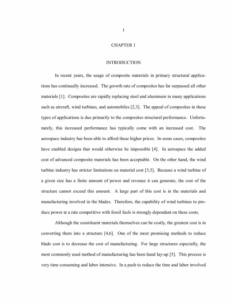
from environmental degradation [2]. Figure 1 is a micrograph of a typical composite ma-
terial from reference 10. The picture is looking along the direction of the fibers of a
D155 fabric at 60X magnification.
6
m 100 µ
Figure 1: Micrograph of fibers and resin [10].
Matrix Materials
Composites utilize many different materials to form the matrix. There are metal
matrix composites, ceramic matrix composites, and polymer matrix composites. The first
two can be very difficult to process, and have been used sparsely for very specific appli-
cations. The most common structural composite materials are fiber reinforced plastics, or
FRPs [11]. These materials typically use one of two types of plastic for the matrix. The
first types are thermosetting plastics such as epoxy, otherwise known as thermosets.
Thermosets are polymer chains infused into the reinforcement in the liquid form where
they then become strongly cross-linked over a short period of time. Due to the cross-
linking, these matrix materials tend to be quite stiff, and are resistant to creep. Unfortu-
7
nately, they can also be very brittle [11,12]. The second type of polymer used is the
thermoplastic such as nylon. Thermoplastics are also combined with the reinforcement in
the liquid form. However, they contain much longer polymeric chains which give them a
very high viscosity. As a result, thermoplastics cannot be used in many of the manufac-
turing processes that thermosets can. The bonding structure is also different in
thermoplastics. They form much weaker secondary bonds to hold the polymer chains
together [11]. For this reason, thermoplastics can be reshaped and reused to some extent.
At the same time, they are also less stiff and prone to creep. One advantage of the
weaker intermolecular bonds is an increase in damage tolerance [2].
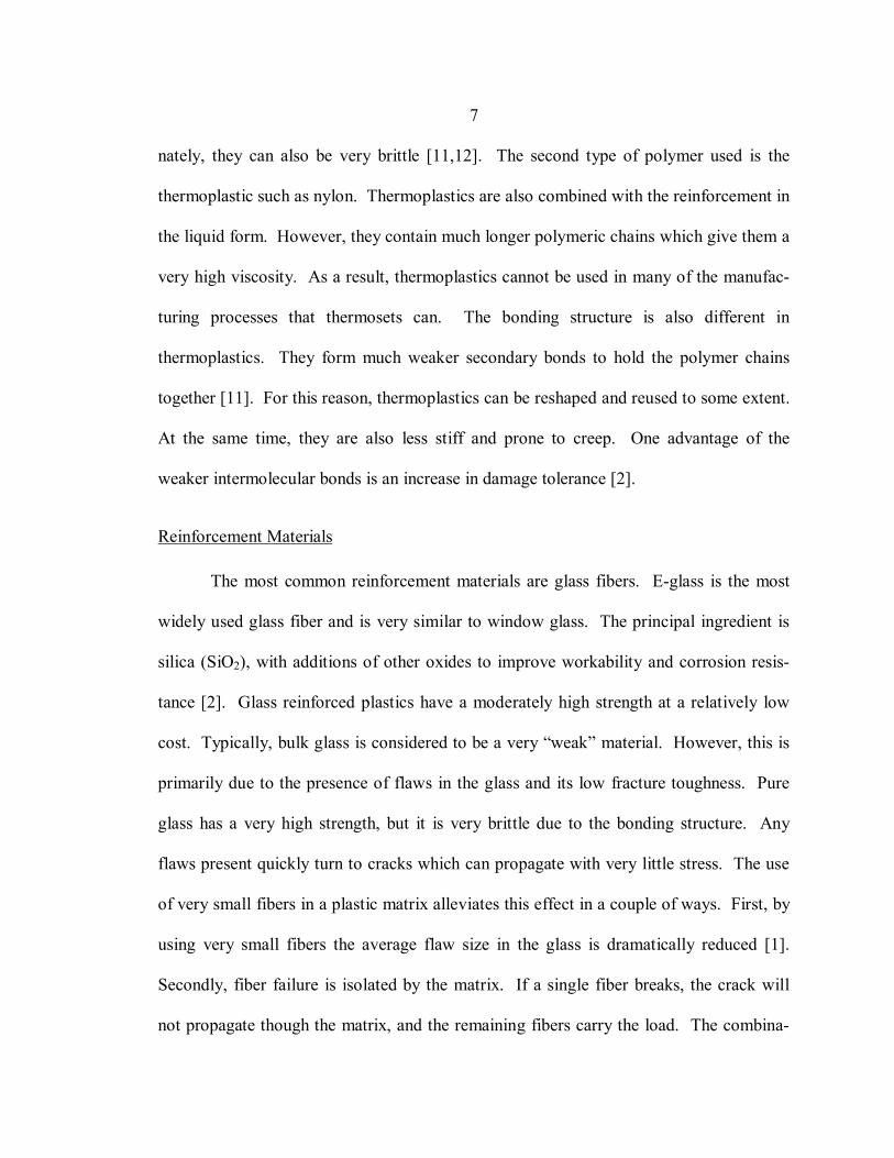
Reinforcement Materials
The most common reinforcement materials are glass fibers. E-glass is the most
widely used glass fiber and is very similar to window glass. The principal ingredient is
silica (SiO2), with additions of other oxides to improve workability and corrosion resis-
tance [2]. Glass reinforced plastics have a moderately high strength at a relatively low
cost. Typically, bulk glass is considered to be a very “weak” material. However, this is
primarily due to the presence of flaws in the glass and its low fracture toughness. Pure
glass has a very high strength, but it is very brittle due to the bonding structure. Any
flaws present quickly turn to cracks which can propagate with very little stress. The use
of very small fibers in a plastic matrix alleviates this effect in a couple of ways. First, by
using very small fibers the average flaw size in the glass is dramatically reduced [1].
Secondly, fiber failure is isolated by the matrix. If a single fiber breaks, the crack will
not propagate though the matrix, and the remaining fibers carry the load. The combina-
8
tion of fibers and matrix also spreads damage over a large area, which can dissipate a
large amount of energy. These effects, among others, make fiberglass very strong and
damage tolerant. Among composite materials, fiberglass also has one of the lowest costs
[1]. The limitations of fiberglass are primarily due to its high density and low tensile
modulus [2].
Carbon fibers are the second most common reinforcement, and boast one of the
highest strength and stiffness to weight ratios of any material. Its primary use has been in
the aerospace industry, although it is becoming more widely used in all fields. It has seen
increased usage in sporting goods especially, for items such as bicycle frames and tennis
rackets [2]. Carbon fiber also has very good fatigue resistance which is important in
many designs, especially wind turbines [10]. The primary drawback of carbon fiber is
the cost. Bulk glass fibers are produced for around $2/kg, while the lowest cost carbon
fibers are currently about $19.80/kg [5]. This has limited the use of carbon fiber in many
industries, and will continue to do so in the future. Another weakness of carbon fiber is
due to its high degree of anisotropy. Because the fibers are typically oriented in a single
direction or plane, the part is very stiff in that direction, but not in the other planes. For
this reason, any waviness or misalignment of the fibers can cause high stress concentra-
tions. This is particularly true in compression where any defect can greatly reduce the
compressive strength [13].
Glass and carbon fibers are typically used in the form of fiber mats. These mats
are created by weaving bundles of fibers called tows into a fabric, much like a textile
process. By altering the directions of the fiber tows, fabrics with very different properties
9
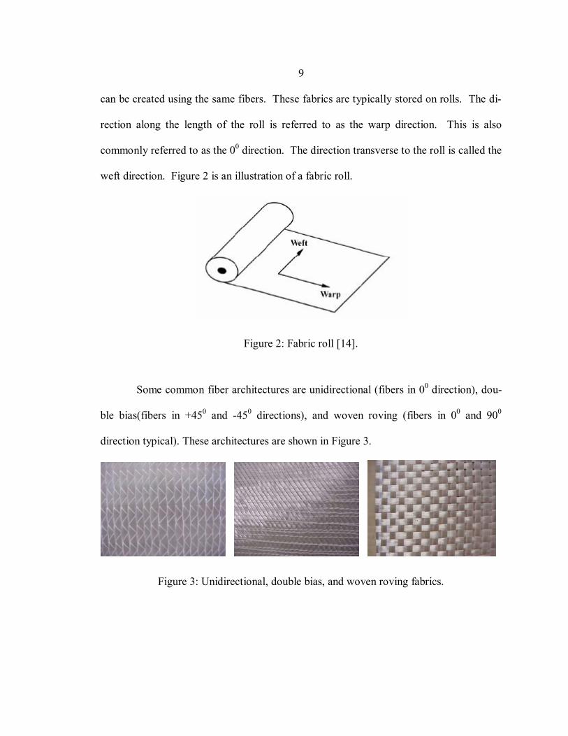
can be created using the same fibers. These fabrics are typically stored on rolls. The di-
rection along the length of the roll is referred to as the warp direction. This is also
commonly referred to as the 00 direction. The direction transverse to the roll is called the
weft direction. Figure 2 is an illustration of a fabric roll.
Figure 2: Fabric roll [14].
Some common fiber architectures are unidirectional (fibers in 00 direction), dou-
ble bias(fibers in +450 and -450 directions), and woven roving (fibers in 00 and 900
direction typical). These architectures are shown in Figure 3.
Figure 3: Unidirectional, double bias, and woven roving fabrics.
10
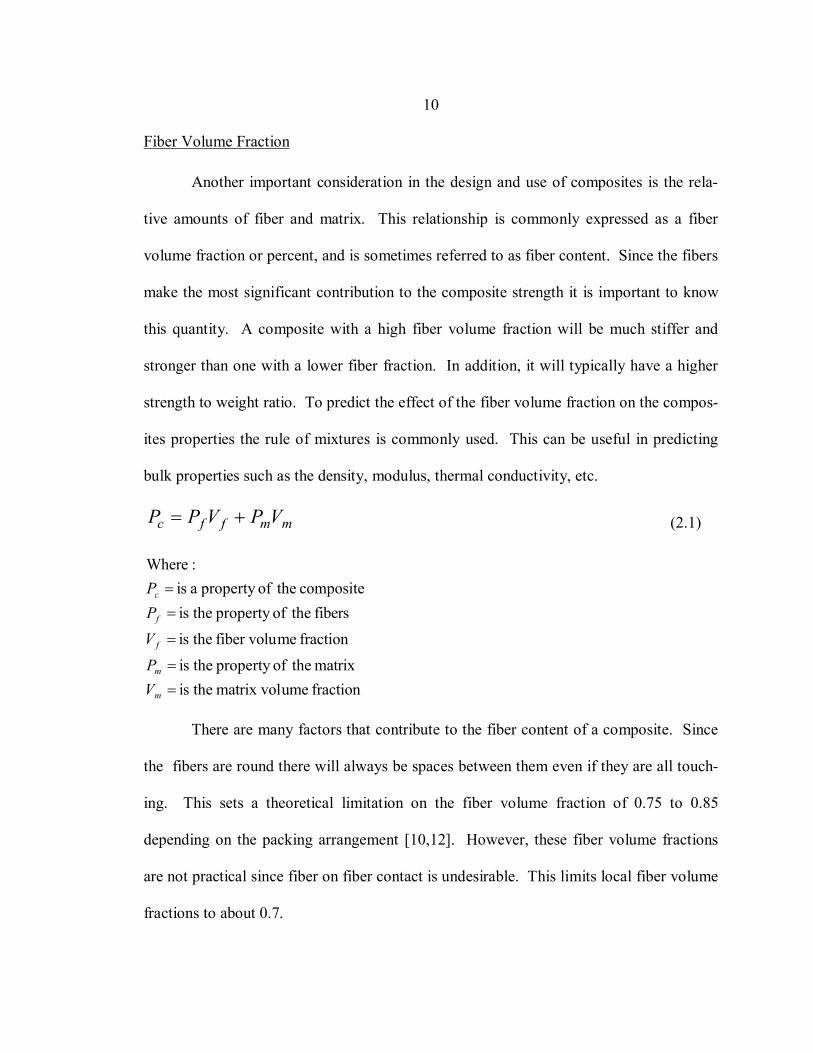
Fiber Volume Fraction
Another important consideration in the design and use of composites is the rela-
tive amounts of fiber and matrix. This relationship is commonly expressed as a fiber
volume fraction or percent, and is sometimes referred to as fiber content. Since the fibers
make the most significant contribution to the composite strength it is important to know
this quantity. A composite with a high fiber volume fraction will be much stiffer and
stronger than one with a lower fiber fraction. In addition, it will typically have a higher
strength to weight ratio. To predict the effect of the fiber volume fraction on the compos-
ites properties the rule of mixtures is commonly used. This can be useful in predicting
bulk properties such as the density, modulus, thermal conductivity, etc.
mmffc VPVPP += (2.1)
fraction umematrix vol theis matrix theofproperty theis
fraction mefiber volu theis fibers theofproperty theis
composite theofproperty a is :Where
==
=
==
m
m
f
f
c
VPVPP
There are many factors that contribute to the fiber content of a composite. Since
the fibers are round there will always be spaces between them even if they are all touch-
ing. This sets a theoretical limitation on the fiber volume fraction of 0.75 to 0.85
depending on the packing arrangement [10,12]. However, these fiber volume fractions
are not practical since fiber on fiber contact is undesirable. This limits local fiber volume
fractions to about 0.7.
11
In woven or stitched fabrics the maximum attainable fiber volume fraction is re-
duced even more. Although the fiber volume fraction within the tows may be 0.7, there
are larger gaps created between tows by the weaving and stitching pattern. Resin flow
channels may also be integrated into the fabric that can lower the fiber volume fraction.
The fiber volume fractions of fabrics can be increased by forcing the plies together with
mechanical force [10]. This can be accomplished by a hard tool surface, or by a fluid
pressure. As pressure is applied, the fibers get mashed into each other, shrinking the
voids caused by stitching. This is referred to as nesting, and will be described in greater
detail later.
Porosity
Porosity has a couple of meanings in relation to composites. The first, in the ab-
sence of resin, is simply the opposite of the fiber volume fraction, or one minus the fiber
volume fraction. This value is more relevant to flow modeling than strength concerns.
For flow modeling one is more concerned about the passage ways between the fibers than
the fibers themselves. The other meaning of porosity is in relation to microscopic voids
or air pockets existing in a composite after the impregnation by the resin. This type of
porosity can be detrimental to the mechanical performance of a part. Porosity can cause
stress concentrations, as well as allow fibers to rub against each other. This is especially
important for fatigue properties. Porosity can also leave the fibers exposed to harmful
environments [2]. One of the best ways to reduce porosity is to use a vacuum to pull the
air out of a mold. As the resin is injected, there is little air to trap.
12
Manufacturing Processes
There are many techniques available today for manufacturing thermoset compos-
ite parts. Some are still very low tech and labor intensive, while some involve very
sophisticated tooling and computer controls. However, all of these processes share some
of the same challenges and requirements. They all consist of a tool to hold the fabric in
the correct position while the resin is curing, and require some means of forcing the resin
into the fabric. The major differences in the processes are the resulting part quality, limi-
tations in size and geometry, cost of tooling, and process time.
The most basic and labor intensive process is known as hand lay-up. In hand lay-
up fabric is placed onto a tool where resin is applied by hand using rollers and squeegees.
Each ply must be saturated as it is applied to the tool to ensure that no bubbles are left
between plies. This makes hand lay-up very time consuming, but it does have its advan-
tages. Carefully applying resin to each ply can ensure a part without dry spots.
Unfortunately, the process is not performed under vacuum so micro-porosity is possible.
Hand lay-up is very attractive due to the low cost of the tooling required. Since there is
no pressure applied to the tool it does not have to be very robust, and can be made out of
a variety of materials. In many cases, the tool will only have one side to produce a nice
finish on the outside of the part. Hand lay-up can also be used to produce very large
parts. As long as there are enough people to apply the resin to the fabric before it cures,
there are really no limitations on the size of the part. Hand lay-up is currently the most
utilized method of manufacture for large wind turbine blades [5]. Unfortunately, there
are also many disadvantages to hand lay-up. The most obvious is the labor cost. In addi-
13
tion, the application of the resin in an open environment allows very volatile emissions to
escape from the resin that can be harmful to humans and to the environment [14]. It is
anticipated that the use of hand lay-up for wind turbines will eventually be restricted due
to the high volume of emissions [5]. Other disadvantages are lower dimensional toler-
ances, poor fatigue performance, and less aerodynamic surfaces. Even with these
considered, hand lay-up is still the fastest and cheapest way to produce a small number of
composite parts with few defects, but the process is limited.
Beginning in the 1950’s, more industrialized processes began to evolve for use on
aircraft [1,15]. These processes are generally referred to as resin transfer molding proc-
esses, or RTM. In RTM the fabric is laid into a tool where the resin is forced into the
fabric under pressure. These processes have several advantages over the hand lay-up
process. The process has the potential to be more repeatable and consistent since the hu-
man involvement is reduced. This reduction in human involvement also reduces labor
costs. In addition, the amount of volatile emissions is reduced. Much higher fiber con-
tents can also be achieved since the tool can clamp down on the fiber preform.
Dimensional tolerances can also be increased if the tool is two sided [16]. The disadvan-
tages are the cost of the mold and the difficulty in forcing the resin through the fabric.
Modifications of the RTM process have been developed recently that reduce these
disadvantages. Although there are many variants being used today, they all deal with
these problems in a similar manner. Lower tool costs are achieved with the use of one-
sided molds. In these processes a vacuum is drawn on the fabric, while a flexible bag-
ging is forced against the preform by atmospheric pressure. To deal with the problem of
14
getting the resin to flow large distances through the fabric, a distribution network is used.
This distribution network allows the resin to flow through high permeability channels or
layers to disperse it throughout the mold. The resin must then flow a much shorter dis-
tance in the plane or though the thickness of the part. Several variants of these processes
are described in detail by Larson [17], and will be discussed briefly here.
One process that has been successfully used on large structures is the Seemanns
Composite Resin Infusion Molding Process (SCRIMP™). This process has been used
since the 1980’s and its use continues to increase. There are several variations of
SCRIMP™. One uses a series of channels above the fabric for resin distribution, and the
resin is then forced to flow in the plane of the fabric between the channels. In other vari-
ants, a high permeability layer may be placed over the fabric for resin distribution. The
resin is then forced to flow though the thickness of the fabric. This layer is then peeled
off after the process is complete. SCRIMP™ is capable of producing large parts very
quickly, cheaply, and with high fiber volume fractions [7].
A very similar process known as the Fast Remotely Actuated Channeling process
(FASTRAC) is a more recent variation of this general principle. The main difference in
the FASTRAC process compared to SCRIMP™ is a more refined distribution strategy.
The distribution network is created by a “FASTRAC layer” which is a flexible membrane
with tightly spaced channels formed into it. The major difference is that these channels
can be collapsed to force the extra resin though the fabric or out of the mold, rather than
leaving them attached to the part as in SCRIMP™. The FASTRAC layer also allows a
positive pressure to be applied to the fabric to achieve even higher fiber volume fractions.
15
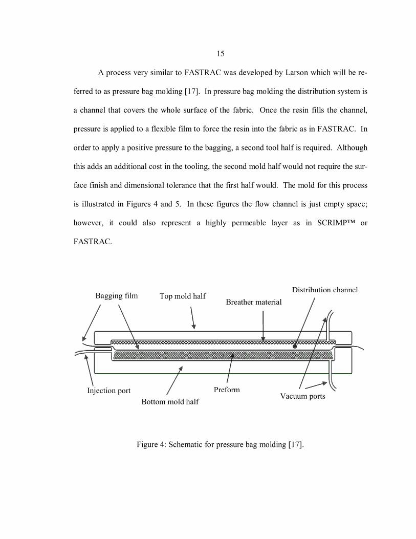
A process very similar to FASTRAC was developed by Larson which will be re-
ferred to as pressure bag molding [17]. In pressure bag molding the distribution system is
a channel that covers the whole surface of the fabric. Once the resin fills the channel,
pressure is applied to a flexible film to force the resin into the fabric as in FASTRAC. In
order to apply a positive pressure to the bagging, a second tool half is required. Although
this adds an additional cost in the tooling, the second mold half would not require the sur-
face finish and dimensional tolerance that the first half would. The mold for this process
is illustrated in Figures 4 and 5. In these figures the flow channel is just empty space;
however, it could also represent a highly permeable layer as in SCRIMP™ or
FASTRAC.
Top mold half Bagging film Breather material
Bottom mold half Injection port
Vacuum ports Preform
Distribution channel
Figure 4: Schematic for pressure bag molding [17].
16
Resin pools near the injection port
No net pressure on bagging film during injection
Bagging film displaces to allow channel formation Vacuum
Vacuum
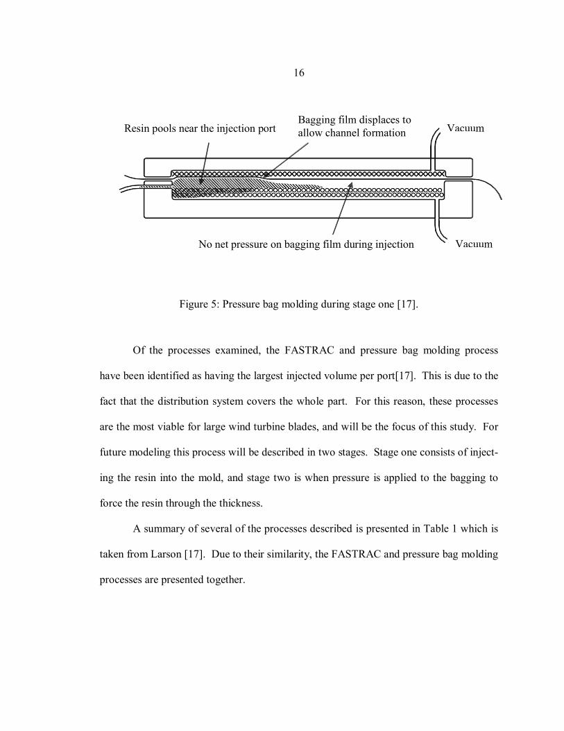
Figure 5: Pressure bag molding during stage one [17].
Of the processes examined, the FASTRAC and pressure bag molding process
have been identified as having the largest injected volume per port[17]. This is due to the
fact that the distribution system covers the whole part. For this reason, these processes
are the most viable for large wind turbine blades, and will be the focus of this study. For
future modeling this process will be described in two stages. Stage one consists of inject-
ing the resin into the mold, and stage two is when pressure is applied to the bagging to
force the resin through the thickness.
A summary of several of the processes described is presented in Table 1 which is
taken from Larson [17]. Due to their similarity, the FASTRAC and pressure bag molding
processes are presented together.
17
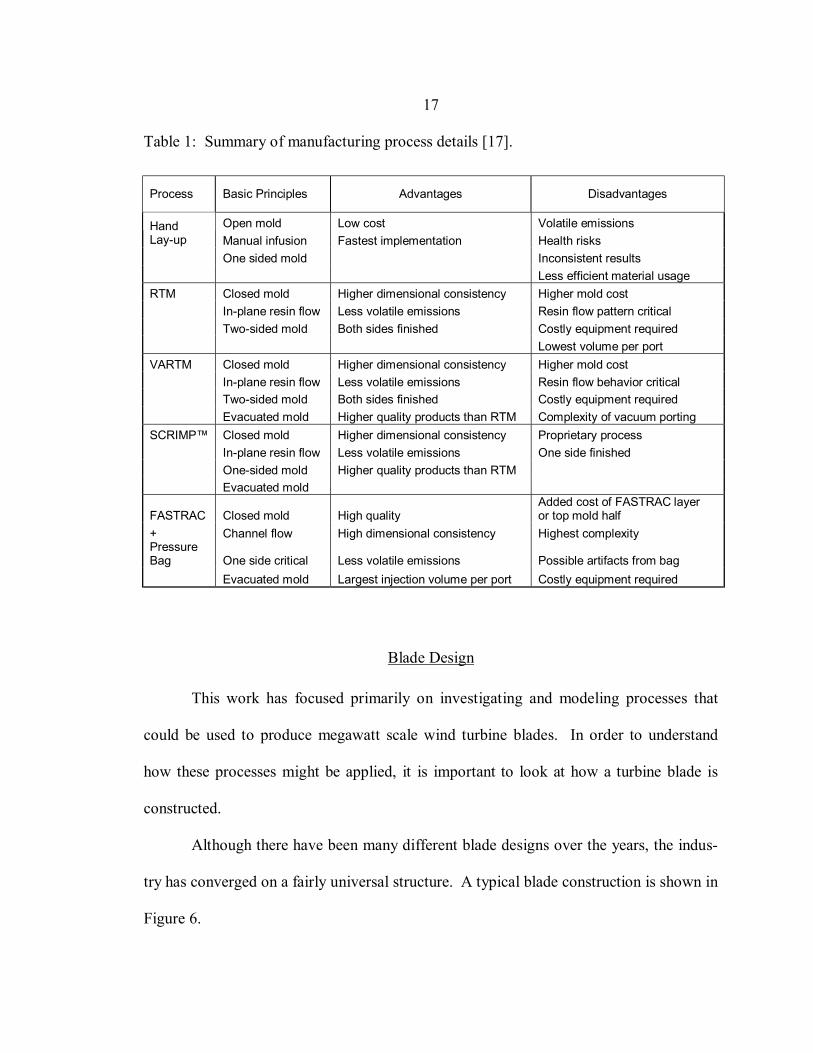
Table 1: Summary of manufacturing process details [17].
Process Basic Principles Advantages Disadvantages
Open mold Low cost Volatile emissions Hand Lay-up Manual infusion Fastest implementation Health risks One sided mold Inconsistent results Less efficient material usage RTM Closed mold Higher dimensional consistency Higher mold cost In-plane resin flow Less volatile emissions Resin flow pattern critical Two-sided mold Both sides finished Costly equipment required Lowest volume per port VARTM Closed mold Higher dimensional consistency Higher mold cost In-plane resin flow Less volatile emissions Resin flow behavior critical Two-sided mold Both sides finished Costly equipment required Evacuated mold Higher quality products than RTM Complexity of vacuum porting SCRIMP™ Closed mold Higher dimensional consistency Proprietary process In-plane resin flow Less volatile emissions One side finished One-sided mold Higher quality products than RTM Evacuated mold
FASTRAC Closed mold High quality Added cost of FASTRAC layer or top mold half
+ Channel flow High dimensional consistency Highest complexity Pressure Bag One side critical Less volatile emissions Possible artifacts from bag Evacuated mold Largest injection volume per port Costly equipment required
Blade Design
This work has focused primarily on investigating and modeling processes that
could be used to produce megawatt scale wind turbine blades. In order to understand
how these processes might be applied, it is important to look at how a turbine blade is
constructed.
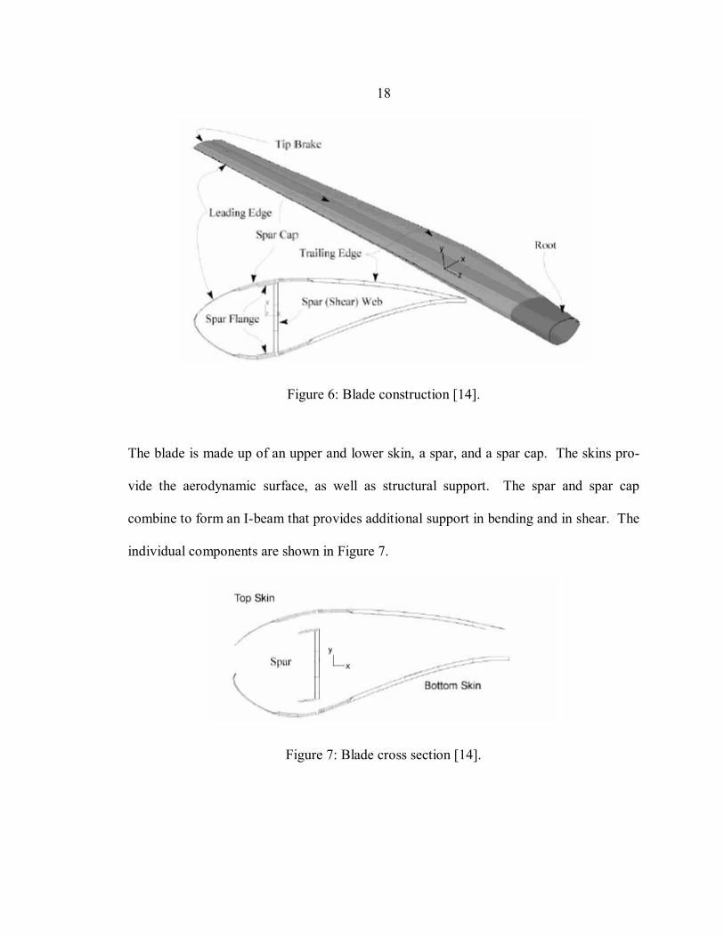
Although there have been many different blade designs over the years, the indus-
try has converged on a fairly universal structure. A typical blade construction is shown in
Figure 6.
18
Figure 6: Blade construction [14].
The blade is made up of an upper and lower skin, a spar, and a spar cap. The skins pro-
vide the aerodynamic surface, as well as structural support. The spar and spar cap
combine to form an I-beam that provides additional support in bending and in shear. The
individual components are shown in Figure 7.
Figure 7: Blade cross section [14].

19
The most common materials used for turbine blades have been E-glass fibers with
thermoset resins such as epoxy and vinyl-ester [5]. These materials have been used due to
their cost and resistance to fatigue. As blades continue to increase in length, carbon fi-
bers are becoming more important. In some cases, the blades are becoming so long that
if the blade were made strictly of glass fibers it would fail under its own weight. The
high strength and stiffness to weight ratio make carbon fiber a potential solution to this
problem [5]. Although carbon fiber is more expensive, there are potential benefits that
could come with its use that might offset this material cost.
20
CHAPTER 3
PROCESS MODELING BACKGROUND
Producing a successful part using RTM can be very challenging. Due to complex
geometry, and the anisotropic permeability of the fabrics used, predicting the flow front
though a mold is a difficult problem. As mentioned before, this is commonly done by
experts who rely heavily on experience. A trial and error process is also used to detect
and eliminate problems involving mold construction. In one such method a partial charge
of resin is injected and allowed to set up. This is repeated using progressively more resin
to create a series of parts with a progressing flow front. This process is very useful in
identifying where vents need to be located or where more injection ports are required.
For smaller parts, the cost of doing this may be insignificant as long as a new mold is not
required. For parts where the absolute minimum process time is critical, as in automotive
manufacturing processes, flow modeling is becoming more essential. This is also true for
large parts where waste can have a significant cost and molds are very expensive. The
best time to make changes to the design of a mold is before it is built.
Process modeling has been used with varying success for many years now. The
liquid injection molding software (LIMS) developed by the University of Delaware is a
modeling software that has been used to successfully model complex 2D parts [18,19].
This program is also developing means to model channels and account for fabric com-
pression, as in more modern processes [20]. One advantage of this program is that it can
use a finite element mesh generated by PATRAN so complex geometries can be modeled
[18,20].
21
Unfortunately, even using commercially available software can be difficult for
complex one-sided molding processes. Some existing finite element programs such as
ABAQUS also have porous media fluid elements capable of orthotropic or anisotropic
permeability tensors. For closed mold processes, this program could be used to model
complex three dimensional geometries with little additional programming. However, for
one-sided molding processes there would still need to be a large amount of manual pro-
gramming. Other programs have been developed independently to model processes such
as SCRIMP™ and VARTM [7,21,22,23]. These programs also use a finite element con-
trol volume technique to model the process. Changes in fabric properties during the
process, as well as the resin distribution channels, are included in the models. However,
they still result in a two dimensional model where the resin flows in the plane of the fab-
ric between channels.
As was pointed out earlier, the processes with the greatest capability for very
large parts are where the distribution channel covers the whole surface and the flow is
though the thickness. No models were found that handle this type of process specifically.
The goal of this work was to select and model a process that would be optimal for creat-
ing a large wind turbine blade. Due to the geometry of the upper and lower skins of the
blade, it was decided that a flat rectangular plate would be a good approximation of the
geometry for this study. Although not exact, it reduces the complexity of the problem by
an order of magnitude by permitting a 2D model. In addition to being much easier to
program, it is also very fast to run. This aids in examining how changing process pa-
rameters can influence the process. This geometry also lends itself to finite difference, or
22
control volume techniques which are much simpler to program than finite elements. The
specific method used in this work is similar to the Hardy Cross method for analyzing pip-
ing systems [24]. The development of the control volume technique used in this study
will be discussed in detail in the following sections.
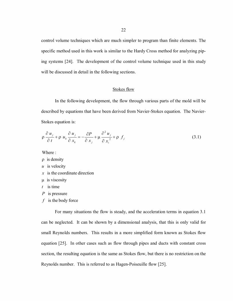
Stokes flow
In the following development, the flow through various parts of the mold will be
described by equations that have been derived from Navier-Stokes equation. The Navier-
Stokes equation is:
ji
j
jk
jk
j fx
uxP
xu
ut
uρµρρ
∂
∂+
∂∂
−=∂
∂+
∂
∂2
2
+ (3.1)
forcebody theis pressure is
timeis viscosityis
direction coordinate theis velocityis density is
:Where
fPt
xu
µ
ρ
For many situations the flow is steady, and the acceleration terms in equation 3.1
can be neglected. It can be shown by a dimensional analysis, that this is only valid for
small Reynolds numbers. This results in a more simplified form known as Stokes flow
equation [25]. In other cases such as flow through pipes and ducts with constant cross
section, the resulting equation is the same as Stokes flow, but there is no restriction on the
Reynolds number. This is referred to as Hagen-Poiseuille flow [25].
23
ji
j
j
fx
uxP
ρµ +∂
∂+
∂∂
−= 2
2
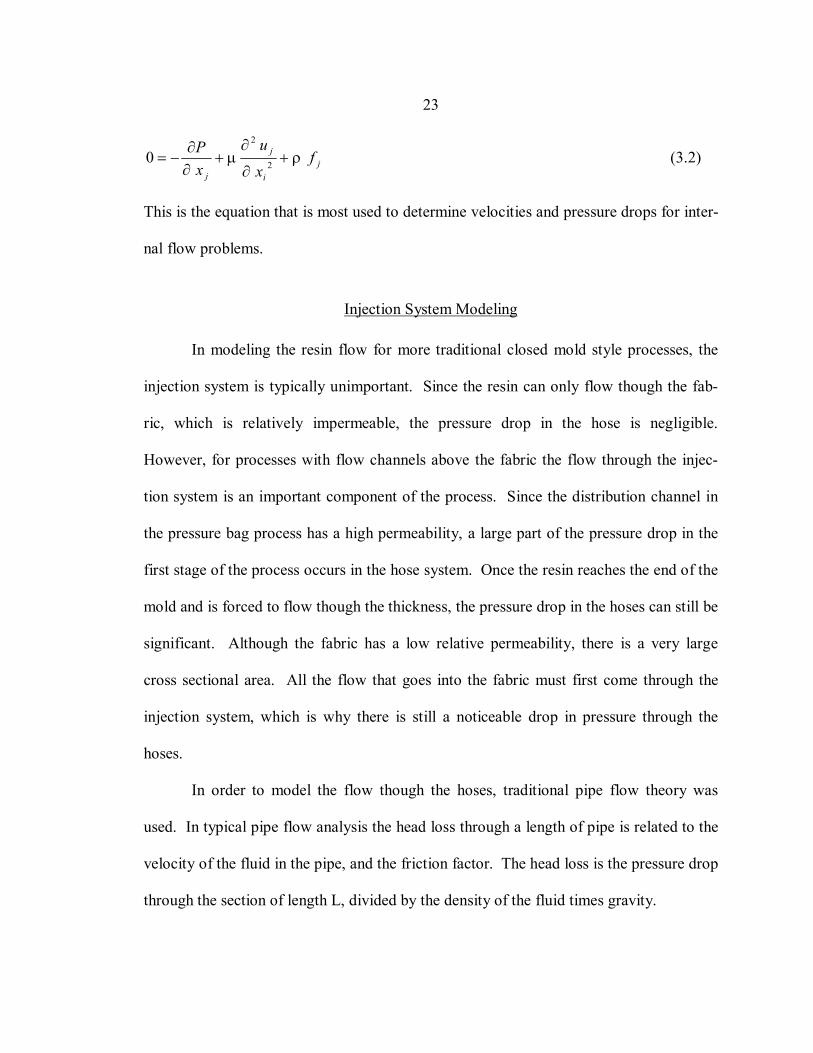
0 (3.2)
This is the equation that is most used to determine velocities and pressure drops for inter-
nal flow problems.
Injection System Modeling
In modeling the resin flow for more traditional closed mold style processes, the
injection system is typically unimportant. Since the resin can only flow though the fab-
ric, which is relatively impermeable, the pressure drop in the hose is negligible.
However, for processes with flow channels above the fabric the flow through the injec-
tion system is an important component of the process. Since the distribution channel in
the pressure bag process has a high permeability, a large part of the pressure drop in the
first stage of the process occurs in the hose system. Once the resin reaches the end of the
mold and is forced to flow though the thickness, the pressure drop in the hoses can still be
significant. Although the fabric has a low relative permeability, there is a very large
cross sectional area. All the flow that goes into the fabric must first come through the
injection system, which is why there is still a noticeable drop in pressure through the
hoses.
In order to model the flow though the hoses, traditional pipe flow theory was
used. In typical pipe flow analysis the head loss through a length of pipe is related to the
velocity of the fluid in the pipe, and the friction factor. The head loss is the pressure drop
through the section of length L, divided by the density of the fluid times gravity.
24
gDvLfh
hosef 2
2
= (3.3)
gPh f ρ
∆= (3.4)
gravity is density fluid theis
section theoflength theis hose theofdiameter theis
velocityaverage theis factorfriction theis
loss head theis :Where
g
LDvf
h
hose
f
ρ
The friction factor depends on things such as the roughness of the pipe, the diameter, and
the Reynolds number of the flow [26]. For turbulent flow the friction factor must be
looked up on a Moody diagram. For laminar flow, the friction factor is a function of the
Reynolds number only. Because of the high viscosity of the resin used in this study (300
cp), the flow was in the laminar regime in all the cases examined. The equations for the
laminar friction factor and Reynolds number are:
Dlamf
Re64
= (3.5)
µρ hose
DDv
=Re (3.6)
viscosityfluid theis diameteron basednumber Reynolds theis Re
:Where
µD
25
The previous equations were then manipulated into a form that would be more useful in
future modeling. This equation directly relates the average velocity through the pipe to
the pressure drop through a given length of hose.
LPD
v hose ∆=
µ32
2
(3.7)
Equation 3.7 can also be derived from the Stokes flow equation. By integrating the
Stokes flow equation and applying the appropriate boundary conditions, the following
equation is formed [26].
( 22
41)( rR
LPrv −
∆=
µ) (3.8)
pipe of radiusouter theis pipe in theposition radial theis
r offunction a as velocity theis )(:Where
Rr
rv
This equation can also be written in terms of the maximum velocity (at r = 0) as:
−= 2
2
max 1)(Rrvrv (3.9)
By integrating equation 3.9 over the cross sectional area, the average velocity through the
pipe can be found to be one half of the maximum velocity. Thus, by equating equations
3.8 and 3.9, and substituting in the diameter and average velocity, equation 3.7 can be
formed. Notice that in equation 3.7 the velocity is proportional to the change in pressure
over a given length. This is similar to the relationship for flow through porous media
where the proportionality is defined by a constant known as the permeability. This will
be discussed more in the following sections.
26
In most applications, the injection system will be more complex involving multi-
ple hoses and hose fittings. In order to find the flow rate though the entire system given a
differential pressure, compatibility and conservation of mass are used. Through conser-
vation of mass the velocity through each component in the system can be related by a
ratio of areas. In order to satisfy compatibility the pressure drop though each section
must add up to the total pressure drop through the entire system. Together, these two
principles can generate an equation to describe the system as a whole.
The system used for this study involved a brass cross fitting with three barbed fit-
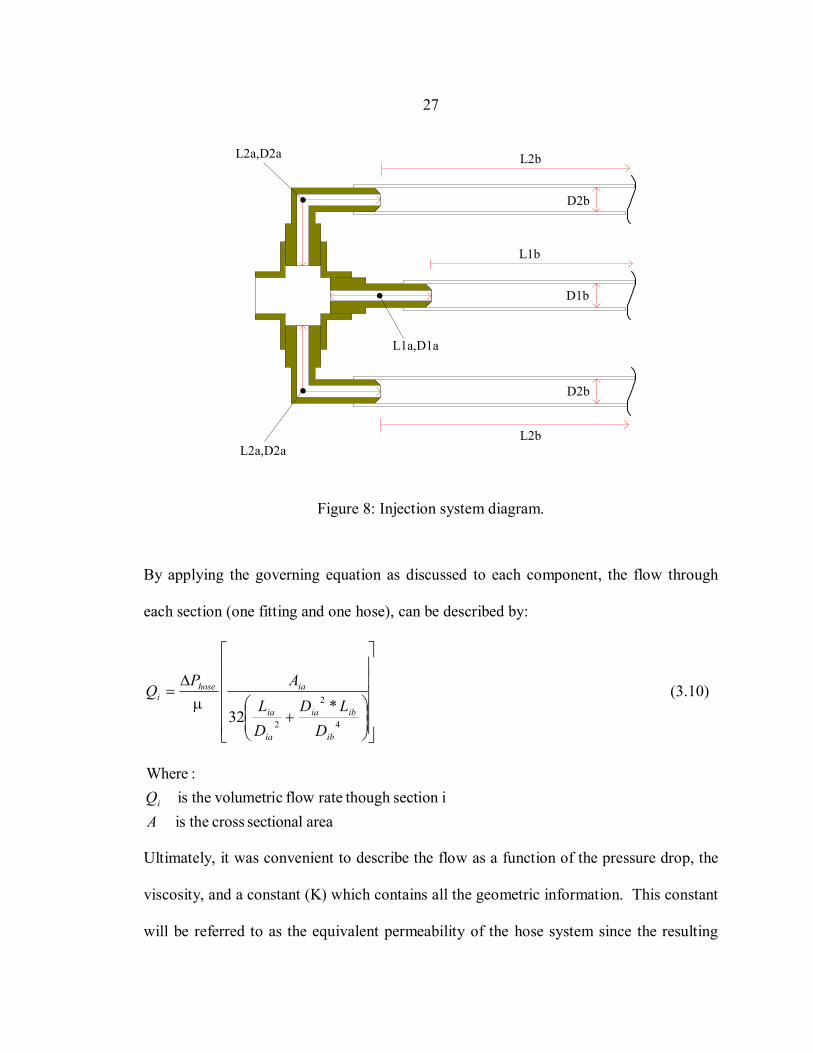
tings and attached hoses. Both 6.35 mm ID and 9.5 mm ID hoses were used. Figure 8 is
a schematic of the hose system as well as the parameters used to determine the flow equa-
tion. A photo of the injection manifold modeled here is presented in the experimental
equipment section. In real piping systems such as this, involving elbows, expansions and
contractions, minor loss terms are typically included to account for any additional pres-
sure drop as a result of these changes. In the cases modeled in this study, the minor loss
terms were found to contribute less than one percent of the total pressure drop and have
been omitted from this analysis for simplicity, but could be included if significant [26].
27
L2b
D2b
L2a,D2a
L1a,D1a
L1b
D1b
L2b
D2b
L2a,D2a
Figure 8: Injection system diagram.
By applying the governing equation as discussed to each component, the flow through
each section (one fitting and one hose), can be described by:
+
∆=
4
2
2
*32
ib
ibia
ia
ia
iahosei
DLD
DL
APQ
µ (3.10)
area sectional cross theis isection though rate flow c volumetri theis
:Where
AQi
Ultimately, it was convenient to describe the flow as a function of the pressure drop, the
viscosity, and a constant (K) which contains all the geometric information. This constant
will be referred to as the equivalent permeability of the hose system since the resulting
28
equation is similar to Darcy’s law [27]. Permeability is typically associated with flow
through porous media. However, for modeling the flow through the hoses, channel, and
fabric simultaneously, the equations must be in an analogous form. Although the physics
involved in the flow through the hoses and fabric are different, the flow through both can
be described by similar equations. The equivalent permeability term is used to lump all
the geometric information together. This term is also different than most permeability
terms because it contains the area and length terms as well. This can be done since the
hoses will be full throughout the process. From equation 3.10, the term in brackets is re-
placed by the equivalent permeability term. This term simply defines the proportionality
between the flux and the driving force as in many transport processes.
ihose
i KPµ
∆=Q (3.11)
Since the three sections of hose are in parallel, the total equivalent permeability is the
sum of the individual permeabilities. It should be noted that permeability is not a resis-
tance, it is a conductivity to flow, so the terms are added directly.
∑=
=n
iihose KK
1 (3.12) hoseni ...3,2,1=
and
∑=
=n
iihose QQ
1 (3.13)
thus
hosehose
hose KP
Qµ
∆= (3.14)
29
Equation 3.14 is the desired result that will be used in subsequent modeling to combine
effects of pipe flow, channel flow and fabric flow in a single model.
Channel Flow Modeling
The next flow regime in the process is through the distribution channel. This part
of the process is again governed by Stokes flow, and has been extensively studied for
many years. An equation similar to that obtained for flow though a circular hose can be
obtained by solving the governing momentum equation. For a circular hose, or for an
extremely thin flat channel, the solution is fairly straightforward. However, for more
complex geometries such as semicircular, triangular, or rectangular the solution can be-
come more difficult. Fortunately, the equations for shapes such as these are presented in
most fluids textbooks. Most involve a term defined as the hydraulic diameter, which is a
ratio involving the cross sectional area and the wetted perimeter. This term is important
in calculating the Reynolds number of the flow. For the rectangular channel used in this
study [26]:
whwh
PA
Dh +==
24 (3.15)
widthchannel theis height channel theis
diameter hydraulic theis perimeter wetted
area sectional cross :Where
whDPA
h
==
30
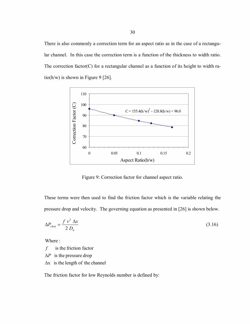
There is also commonly a correction term for an aspect ratio as in the case of a rectangu-
lar channel. In this case the correction term is a function of the thickness to width ratio.
The correction factor(C) for a rectangular channel as a function of its height to width ra-
tio(h/w) is shown in Figure 9 [26].
C = 155.4(h/w)2 - 128.8(h/w) + 96.0
60
70
80
90
100
110
0 0.05 0.1 0.15 0.2
Aspect Ratio(h/w)
Cor
rect
ion
Fact
or (C
)
Figure 9: Correction factor for channel aspect ratio.
These terms were then used to find the friction factor which is the variable relating the
pressure drop and velocity. The governing equation as presented in [26] is shown below.
hchan D
xvfP2
2 ∆=∆ (3.16)
channel theoflength theisx drop pressure theis factorfriction theis
:Where
∆∆Pf
The friction factor for low Reynolds number is defined by:
31
h
CfRe
= (3.17)
number Reynolds theis Reratioaspect given afor constant theis
:Where
h
C
For the rectangular channel, the Reynolds number is defined as:
µρ h
hDv
=Re (3.18)
This equation was then rearranged into a more useful form as in the case of the hose sys-
tem. Again, the desired equation was one relating the flow rate to the gradient in
pressure, and a constant containing the geometric information. The resulting equations
are:
chan
chanchanchanchan x
PKAQ
∆∆
=µ
(3.19)
and
CD
K hchan
22
= (3.20)
channel theofy permabilit equivalent theis area sectional cross theis
rate flow volume theis :Where
chan
chan
chan
KAQ
This technique of generating an equivalent permeability of a channel has been ex-
amined by Hammami, et al., for modeling the edge effect in conventional RTM [28].
Their study also examined the effect of the simultaneous flow into the fabric as the resin
is flowing into the channel. The flow of the fluid into the fabric changes the velocity pro-
32
file in the channel, and thus the equivalent permeability. For cases where the channel is
very small and the permeability of the fabric is large, they found that the effect of the
transverse flow into the fabric dramatically changed the flow though the channel. In or-
der to quantify when this effect needs to be accounted for, they introduced a transverse
flow factor which was defined as:
2
12d
mkz=η (3.21)
with x
z
kk
m = (3.22)
tiespermeabili of ratio a is direction flow in thetiy permeabili fabric theis
direction transvesein thety permeabili fabric theis height channel theis
factor flow e transvers theis :Where
mkkd
x
z
η
It was experimentally determined that for values of η < 5E-4 that the transverse flow into
the fabric could be neglected. For the cases examined in this study the permeabilities are
sufficiently small that the transverse flow can be neglected, thus equation 3.20 is valid.
Fabric Flow Modeling
Darcy Flow
The flow of resin through the fabric is governed by Darcy’s law [27], which is
very similar to the resulting equation for channel flow. Darcy’s law expresses the flow of
the fluid through the fabric by relating the velocity to the pressure drop, and the fabric
33
permeability which is a conductance to flow. The permeability is actually a second order
tensor, meaning its value depends on the direction of the flow. For one dimensional flow
through the thickness, Darcy’s law is:
dzdPK
v z
µ−= (3.23)
gradient pressure theis
direction z in they permabilit fabric theis :Where
dzdPK z
For flow through the fabric, it is extremely difficult to calculate the permeability constant
(K) by knowing only the geometric information. Micro-models exist for estimating the
permeability of a fabric given fiber diameters, fiber spacing, and other relevant informa-
tion [6,29,30]. However, these models are very complex and have varying accuracy. In
addition, there must still be tests performed in order to determine some of the parameters
needed as input to the models. The most accurate and direct way to determine the per-
meability is through testing. By knowing the velocity, pressure drop, and viscosity of a
fluid moving through a fabric the permeability can be calculated. Because most RTM
modeling has been done for closed mold processes, the permeability in the plane of the
fabric was typically of the greatest concern [8,18,31,32,33]. For this reason, the majority
of available permeability data is for flow in the plane. For the two-stage processes such
as pressure bag molding and FASTRAC, the most important value is the permeability
through the thickness. This is because the distribution channel covers the surface of the
fabric so all the in-plane flow occurs in the channel and the flow in the fabric is primarily
though the thickness. For a process such as SCRIMP™ where there may be a large spac-
34
ing between the flow channels the in-plane permeability would be more important. The
in-plane permeability can be either higher or lower than the through thickness value de-
pending on the fabric type and compaction pressure. Parnas et al. have found in general
the in-plane permeability in the direction of the fibers is 6-8 times larger than it is for
through the thickness [34]. However, if the flow in the plane is transverse to the fibers
the permeability could be expected to be close to the through thickness value or possibly
even less.
Saturated vs. Unsaturated Flow
Darcy’s law was originally intended for modeling saturated flow of water through
soil [27]. Because of this, it has some deficiencies when modeling unsaturated flow
though a fabric. In order to use it to model this type of flow it must be modified slightly.
In calculating the permeability, the velocity is determined by dividing the flow rate by the
cross sectional area. The area used is the total flow area of the fabric. This means that
the velocity in Darcy’s law is the superficial velocity, or the velocity averaged over the
whole area. Due to the presence of the fabric, the actual flow area is less than the total
area. This means that the actual velocity of the fluid through the preform is higher than
the superficial velocity because the flow area is reduced. This reduction in flow area can
be determined by knowing the fiber volume fraction of the fabric. Actually, the term
commonly used is called the porosity (e) of the fabric which is one minus the fiber vol-
ume fraction. The modified equation becomes:
dzdP
eK
v zactual µ
−= (3.24)
35
Another additional term required to model unsaturated flow is the capillary pressure.
This is a consequence of the wicking behavior of the fabric caused by surface tension.
This tends to pull the resin along, which results in a higher apparent pressure than the ap-
plied pressure. The -dP term will be replaced by ∆P, recognizing the pressure drop is
linear, and that the flow occurs from high to low pressure. Darcy’s law is modified ac-
cordingly.
dzPP
eK
v capappz )( +∆=µ
(3.25)
pressurecapillary theis pressure fluidin drop theis
:Where
capPPapp∆
The capillary pressure is dependant on properties of the fabric and the resin. One equa-
tion for determining the surface tension as presented by [35] is
θσ cos1e
eDFP
fcap
−= (3.26)
angle wetting theis os tensionsurface theis
fiber a ofdiameter theis factor form theis
:Where
θσc
DF
f
The fiber diameter, porosity, and form factor are all properties of the fabric, while the
surface tension is a property of the resin. The wetting angle is a property of the resin and
fabric. Its value can vary depending on the measurement method [35]. For the most ac-
curate results in an infusion process, the dynamic contact angle is the most appropriate
[36]. It is measured as the fluid is moving in relation to the solid interface. Both an ad-
36
vancing and receding angle can be determined. However, the static contact angle gives a
very good approximation for the resin systems used in RTM, and is easier to measure
[36]. Fortunately, the wetting angle is only dependent on the fabric material and not on
the fabric architecture. Therefore, once the fabric properties are known for a given fab-
ric, the capillary pressure can be calculated for any resin with that fabric if its surface
tension and wetting angle are known. The form factor depends on the fabric architecture
and whether the flow is along the fibers or transverse. Transverse flow typically has a
form factor with a value from one to two [35]. The porosity is included because as the
porosity decreases, the surface area to volume ratio increases, which increases the capil-
lary pressure. Capillary pressure is not very temperature dependent since both the contact
angle and surface tension are very weak functions of temperature [35,36,37].
Although the capillary pressure is typically much smaller than the injection pres-
sure, it can change the results of a test by a noticeable amount. Some researchers have
claimed that the capillary effect was negligible in their permeability tests while others
have claimed capillary pressures had a significant effect [32,34,35,38,39]. The extent of
this effect is going to vary depending on the fabric, the resin, and the injection pressures.
Luo et al. conducted a study on the capillary pressures of a silicone oil and corn syrup
with a couple of fabrics [39]. The largest capillary pressure they found was approxi-
mately 5 kPa for the silicone oil and was less for the corn syrup although they did not
give a specific value. This is consistent with the result found by Rossell for the capillary
pressure of a polyester resin transverse to the fibers of 3 kPa [18].
37
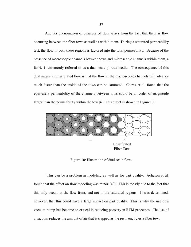
Another phenomenon of unsaturated flow arises from the fact that there is flow
occurring between the fiber tows as well as within them. During a saturated permeability
test, the flow in both these regions is factored into the total permeability. Because of the
presence of macroscopic channels between tows and microscopic channels within them, a
fabric is commonly referred to as a dual scale porous media. The consequence of this
dual nature in unsaturated flow is that the flow in the macroscopic channels will advance
much faster than the inside of the tows can be saturated. Cairns et al. found that the
equivalent permeability of the channels between tows could be an order of magnitude
larger than the permeability within the tow [6]. This effect is shown in Figure10.
UnsaturatedFiber Tow
Figure 10: Illustration of dual scale flow.
This can be a problem in modeling as well as for part quality. Acheson et al.
found that the effect on flow modeling was minor [40]. This is mostly due to the fact that
this only occurs at the flow front, and not in the saturated regions. It was determined,
however, that this could have a large impact on part quality. This is why the use of a
vacuum pump has become so critical in reducing porosity in RTM processes. The use of
a vacuum reduces the amount of air that is trapped as the resin encircles a fiber tow.
38
Fabric Compressibility
Fabric compressibility is very important in all RTM processes, and affects both
the material and processing properties of the part. As the fabric is compressed by fluid
pressure or the mold surface the fibers get compacted and the fiber volume fraction in-
creases. This decreases the thickness of the part, decreases the permeability, and
decreases the porosity. Compressibility is possibly more important to understand in one-
sided molding processes than in closed-mold processes [40]. In a closed mold process
the permeability and fabric thickness are fixed at a certain value which is determined by
the mold gap. Throughout the process the permeability is a constant and independent of
the injection pressure. In one-sided molding processes the compaction of the fabric can
lead to several important phenomena. In processes where the flow is in the plane of the
fabric such as VARTM and SCRIMP™, a part with non-uniform thickness can be created
since the net compaction pressure varies throughout the mold [40].
In processes where the resin is forced though the thickness, the pressure applied to
the fluid is also the pressure compacting the fabric. Therefore, the permeability and fab-
ric thickness can change throughout a process and depend on the pressure at which the
process is taking place. This can create an interesting competing mechanism in these
types of processes. According to Darcy’s law, an increase in pressure will increase the
velocity of the fluid though the fabric. However, increasing the pressure of the fluid will
increase the compaction pressure and lower the permeability. It could be possible in cer-
tain cases for an increase in pressure to increase injection time, although this is not
common. For most fabrics the decrease in thickness tends to compensate for the de-
39
creased permeability in through thickness flow. The effect of compaction on permeabil-
ity is very dependant on the fabric architecture, which means some fabrics are more
affected than others.
Fabric compaction also affects the porosity of the fabric, which will affect the
saturation time for unsaturated flow. This fact adds yet another complication to the prob-
lem. Although permeability decreases with compaction, the decrease in porosity can
increase the velocity of the fluid through a preform. Decreasing the porosity also in-
creases the capillary pressure. However, in most cases these effects are minor.
As a fabric is compressed there are three distinct regimes that have been identified
[15]. The first is where the spacing in the fabric caused by the stitching and weaving is
compressed. This occurs at very low pressures, and results in fiber on fiber contact. This
region is also very linear in nature. In the second regime, both the solid and the voids are
compressed. This is the most complex region, and is the most studied. Very complex
models have been generated to predict the behavior of the fabric in this region. Although
the fibers are touching, they are still moving due to fiber bending, slippage, and nesting
[41]. The third region is where the fabric has been fully compressed. Most fabrics are
fully compressed with 1-2 MPa pressure [15]. In the third regime, all the fibers have
been manipulated into a stable position and cannot be moved any further. The only com-
pression occurring in this regime is due to the solid material compressing. Many fabrics
have compressed to half their original thickness by this point [15].
Overall, the relationships between pressure, ply thickness, and fiber volume frac-
tion are very non-linear. In order to get accurate values for fabric compaction many tests
40
may be required. Typically, the results from these tests can be represented with loga-
rithmic or power law fits [15,42]. However, the results from these fits do not contain any
real physical significance in the parameters used to fit the curves. They may also only fit
limited regions of the data, with problems in extrapolating. Chen et al. have proposed a
method for creating fabric compaction models using four to five parameters [15]. These
parameters are the initial fiber volume fraction, the final fiber volume fraction, the initial
fiber perform bulk compressibility, the fiber compressibility and an empirical index. The
initial and final fiber volume fractions can easily be determined by the areal density, the
fiber density, and the ply thickness.
00 T
sρς
= (3.27)
and f
f Ts
ρς
= (3.28)
density theis thicknessfabric compressedfully theis
thicknessfabric eduncompress theis desity aereal fabric theis
fraction mefiber volu compressedfully theis fraction mefiber volu eduncompress theis
:Where
f
0
f
0
ρ
ς
TT
ss
The fiber compressibility is simply the modulus of the fiber material. The bulk com-
pressibility must be experimentally determined by taking a data point in the first linear
regime. The empirical constant k is the only constant that would require a number of
tests to determine. Fortunately, it has been found that for all the E-glass fabrics tested
and for AS4 carbon that k = 2. This means these fabrics can be represented by only four
41
constants. The procedure for determining and combining these constants is described in
detail in [15]. The resulting equations are:
−=
0
1)(
1TT
TCP
b
(3.29)
and
−=
ss
sCP
b
01)(
1 (3.30)
where
s
k
f
f
b
k
f
f
b C
TTTT
TTs
TTs
C
TTTT
sTT
sTC
−
−
−−−+
−
−
−
−=
0
00000
0
0
00
1
112
1
1
1
1)( (3.31)
and
( )( )( )( )
( )( )( ) sk
f
kf
bkf
kf
b Css
ssssC
sss
ssssC
−
−−−−+
−−
−−=
00
00
12
1
1)( (3.32)
ilitycompressibfiber theis ilitycompressibbulk initial theis
fraction mefiber voluon basedility compressibbulk theis (s)sson thickne basedility compressibbulk theis (T)
pressure compaction theis :Where
s
0
b
b
CCCCP
b
With these formulas, curves for ply thickness and fiber volume fraction versus pressure
can be generated. A similar model has also been developed by Gutowski which also uses
the uncompressed and fully compressed fiber volume fractions [40,43]. This relationship
is described by
42
40
1
1
−
−
=
ss
ss
Af
szσ (3.33)
constant determinedally experimentan is stress compaction theis
:Where
sAzσ
Another phenomenon that is important to be aware of is the viscoelastic behavior
of fiber performs. Bickerton et al. found that dry fiber mats had rate dependant compac-
tion properties, as well as hysteresis [41]. In many manufacturing processes this could
add one more complication to any process modeling. This could be especially important
in SCRIMP™ where the fabric starts in a compressed state, and then is assumed to
bounce back to its uncompressed state as the fabric is saturated. The effect of hysteresis
could mean the fiber mat would not bounce back to its original thickness. This also has
importance in permeability testing which will be discussed later.
Calculating Saturation Time
The ultimate goal of understanding the flow through a fabric is to be able to pre-
dict the time required to saturate a part of a given thickness or length. Although the
process examined here involves more than just flow through the fabric, some valuable
lessons can be learned by looking at the fabric flow independently in one dimension. By
manipulating the modified Darcy equation (equation 3.25) the saturation time required
for a part of a given thickness was created. First it was recognized that
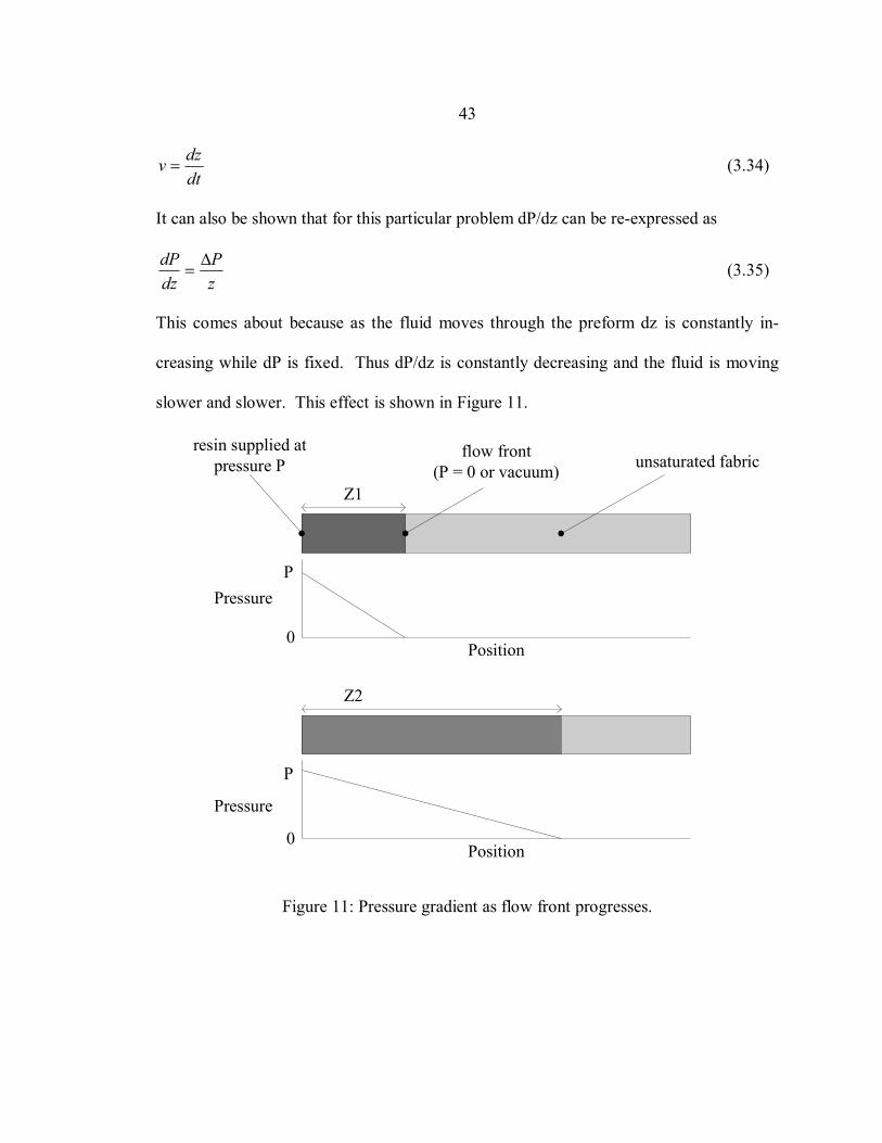
43
dtdzv = (3.34)
It can also be shown that for this particular problem dP/dz can be re-expressed as
zP
dzdP ∆
= (3.35)
This comes about because as the fluid moves through the preform dz is constantly in-
creasing while dP is fixed. Thus dP/dz is constantly decreasing and the fluid is moving
slower and slower. This effect is shown in Figure 11.
Z1
Z2
P
P
0
0
Pressure
Pressure
Position
Position
flow front(P = 0 or vacuum) unsaturated fabric
resin supplied atpressure P
Figure 11: Pressure gradient as flow front progresses.
44
Equation 3.25 can now be expressed as
( )z
PPe
Kdtdz capf +∆
=µ
(3.36)
which can be separated into
dtPPe
Kdzz cap
f )( +∆=µ
(3.37)
Finally, the left side of the equation is integrated from z = 0 to z and the right side is inte-
grated from t = 0 to t giving
tPPe
Kzcap
f )(2
2
+∆=µ
(3.38)
or 2)(
2
fcap KPPezt
+∆=
µ (3.39)
This is a very important result since it shows how the saturation time is a function of the
part thickness or length squared. This is why it is very hard to make long parts when
flowing through the fabric only. This equation can be useful in determining the limiting
cases for RTM processes.
Comprehensive Model
Methodology
The purpose of examining the flow of the resin through the different regions was
to come up with governing equations for each and then combine them in a comprehensive
model. Since resin is flowing though the injection system, distribution channel and fabric
simultaneously, a model was needed that could simulate this interaction. This becomes a
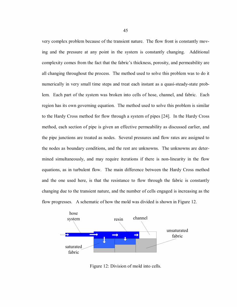
45
very complex problem because of the transient nature. The flow front is constantly mov-
ing and the pressure at any point in the system is constantly changing. Additional
complexity comes from the fact that the fabric’s thickness, porosity, and permeability are
all changing throughout the process. The method used to solve this problem was to do it
numerically in very small time steps and treat each instant as a quasi-steady-state prob-
lem. Each part of the system was broken into cells of hose, channel, and fabric. Each
region has its own governing equation. The method used to solve this problem is similar
to the Hardy Cross method for flow through a system of pipes [24]. In the Hardy Cross
method, each section of pipe is given an effective permeability as discussed earlier, and
the pipe junctions are treated as nodes. Several pressures and flow rates are assigned to
the nodes as boundary conditions, and the rest are unknowns. The unknowns are deter-
mined simultaneously, and may require iterations if there is non-linearity in the flow
equations, as in turbulent flow. The main difference between the Hardy Cross method
and the one used here, is that the resistance to flow through the fabric is constantly
changing due to the transient nature, and the number of cells engaged is increasing as the
flow progresses. A schematic of how the mold was divided is shown in Figure 12.
saturatedfabric
hosesystem channel
unsaturatedfabric
resin
Figure 12: Division of mold into cells.
46
One important simplification to note is that the fabric is only divided along the
length to create fabric columns. These columns are not divided through the thickness.
This is important because it greatly reduces the number of cells required to solve the
problem. If the fabric were divided vertically, a very large number of cells would be re-
quired for accurate results. Since the fabric was not divided into cells, the position of the
fluid front in each cell is stored separately after each time step. The reason that this could
be done for the fabric and not in the channel is because the pressure gradient in the fabric
could be assumed to be linear because the flow in the plane of the fabric is small. For
almost all cases examined, this assumption would cause only very minor error since al-
most all the in-plane flow is taking place in the channel above the fabric. This could not
be done in the channel because as the fluid passes over each column of fabric some of the
fluid enters the fabric. This means the flow rate though the channel is decreasing from
left to right in Figure 12. Since the flow rate is decreasing, the pressure drop is also de-
creasing resulting in a nonlinear pressure profile above the fabric.
Building the Matrix
Because of the transient and non-linear behavior in the problem, all the unknown
flow rates and pressures at each point were determined simultaneously for each time step.
For the real model the channel was broken into many cells. For illustration purposes, the
three cell model of Figure 12 will be used to show how the solution matrix was con-
structed. In order to fully define the problem, four sets of equations were used. These
were compatibility, conservation of mass, the governing flow equations, and the bound-
ary conditions. In order to solve the problem it is important to know the pressures and
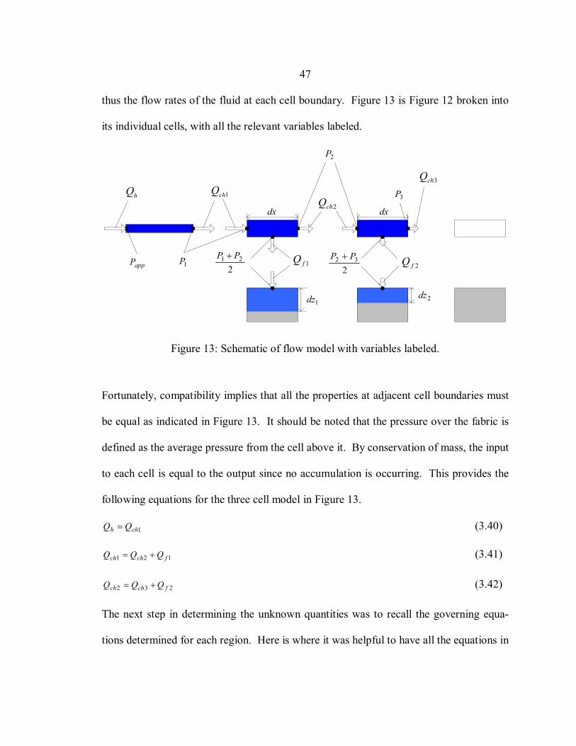
47
thus the flow rates of the fluid at each cell boundary. Figure 13 is Figure 12 broken into
its individual cells, with all the relevant variables labeled.
hQ 1chQ2chQ
3chQ
1P
2P
3P
appP 1fQ2fQ
221 PP +
232 PP +
dx dx
1dz 2dz
Figure 13: Schematic of flow model with variables labeled.
Fortunately, compatibility implies that all the properties at adjacent cell boundaries must
be equal as indicated in Figure 13. It should be noted that the pressure over the fabric is
defined as the average pressure from the cell above it. By conservation of mass, the input
to each cell is equal to the output since no accumulation is occurring. This provides the
following equations for the three cell model in Figure 13.
1chh QQ = (3.40)
121 fchch QQQ += (3.41)
232 fchch QQQ += (3.42)
The next step in determining the unknown quantities was to recall the governing equa-
tions determined for each region. Here is where it was helpful to have all the equations in

48
an analogous form where the flow rate is proportional to the equivalent permeability and
the gradient in pressure. The hose system is treated as a single cell described by
( )µ
1PPKQ apph
h−
= (3.43)
Each cell of the channel is described by
( )dx
PPKAQ chch
ch µ2111
2−
= (3.44)
( )dx
PPKAQ chch
ch µ3222
3−
= (3.45)
And each fabric column is described by
1
21
11
2dz
PPP
KAQ
capff
f
+
+
=µ
(3.46)
2
32
22
2dz
PPP
KAQ
capff
f
+
+
=µ
(3.47)
In order to solve for the unknown values of pressure and flow rate the boundary condi-
tions were also included in the solution matrix. The boundary conditions changed
depending on what point of the process was being looked at.
Before the resin reaches the end of the channel
03 =P (3.48)
Once the resin reaches the end of the channel
04 =chQ (3.49)
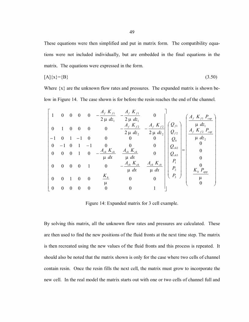
49
These equations were then simplified and put in matrix form. The compatibility equa-
tions were not included individually, but are embedded in the final equations in the
matrix. The equations were expressed in the form.
[A]{x}={B} (3.50)
Where {x} are the unknown flow rates and pressures. The expanded matrix is shown be-
low in Figure 14. The case shown is for before the resin reaches the end of the channel.
=
−
−
−−−−
−−
−−
0
0000
10000000
0000100
010000
0010000001101000001101
22000010
022
00001
2
2
1
1
3
2
1
3
2
2
1
2
2
2
2
1
1
1
1
µ
µ
µ
µ
µµ
µµ
µµ
µµ
apph
capff
capff
ch
ch
h
f
f
h
chchchch
chchchch
ffff
ffff
PK
dzPKA
dzPKA
PPP
QQQQQ
KdxKA
dxKA
dxKA
dxKA
dzKA
dzKAdzKA
dzKA
Figure 14: Expanded matrix for 3 cell example.
By solving this matrix, all the unknown flow rates and pressures are calculated. These
are then used to find the new positions of the fluid fronts at the next time step. The matrix
is then recreated using the new values of the fluid fronts and this process is repeated. It
should also be noted that the matrix shown is only for the case where two cells of channel
contain resin. Once the resin fills the next cell, the matrix must grow to incorporate the
new cell. In the real model the matrix starts out with one or two cells of channel full and
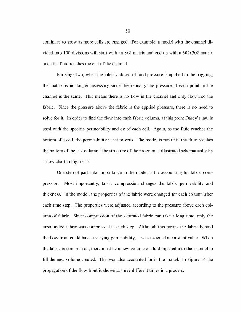
50
continues to grow as more cells are engaged. For example, a model with the channel di-
vided into 100 divisions will start with an 8x8 matrix and end up with a 302x302 matrix
once the fluid reaches the end of the channel.
For stage two, when the inlet is closed off and pressure is applied to the bagging,
the matrix is no longer necessary since theoretically the pressure at each point in the
channel is the same. This means there is no flow in the channel and only flow into the
fabric. Since the pressure above the fabric is the applied pressure, there is no need to
solve for it. In order to find the flow into each fabric column, at this point Darcy’s law is
used with the specific permeability and dz of each cell. Again, as the fluid reaches the
bottom of a cell, the permeability is set to zero. The model is run until the fluid reaches
the bottom of the last column. The structure of the program is illustrated schematically by
a flow chart in Figure 15.
One step of particular importance in the model is the accounting for fabric com-
pression. Most importantly, fabric compression changes the fabric permeability and
thickness. In the model, the properties of the fabric were changed for each column after
each time step. The properties were adjusted according to the pressure above each col-
umn of fabric. Since compression of the saturated fabric can take a long time, only the
unsaturated fabric was compressed at each step. Although this means the fabric behind
the flow front could have a varying permeability, it was assigned a constant value. When
the fabric is compressed, there must be a new volume of fluid injected into the channel to
fill the new volume created. This was also accounted for in the model. In Figure 16 the
propagation of the flow front is shown at three different times in a process.
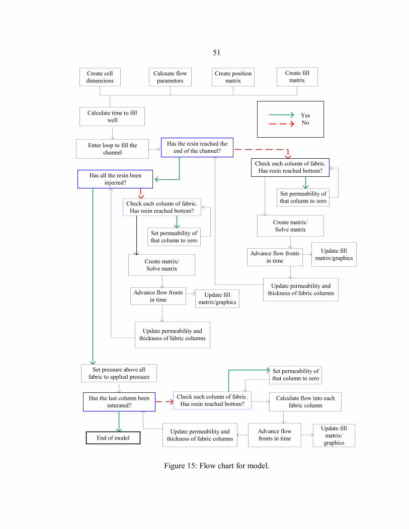
51
Create celldimensions
Calcuate flowparameters
Create positionmatrix
Create fillmatrix
Calculate time to fillwell
Enter loop to fill thechannel
Has the resin reached theend of the channel?
Check each column of fabric.Has resin reached bottom?
Set permeability ofthat column to zero
Create matrix/Solve matrix
Advance flow frontsin time
Update permeability andthickness of fabric columns
Check each column of fabric.Has resin reached bottom?
Set permeability ofthat column to zero
Create matrix/Solve matrix
Advance flow frontsin time
Has all the resin beeninjected?
Set pressure above allfabric to applied pressure
Calculate flow into eachfabric column
Has the last column beensaturated?
Advance flowfronts in time
Update fillmatrix/graphics
Update fillmatrix/graphics
Update fillmatrix/graphics
End of model
YesNo
Check each column of fabric.Has resin reached bottom?
Set permeability ofthat column to zero
Update permeability andthickness of fabric columns
Update permeability andthickness of fabric columns
Figure 15: Flow chart for model.
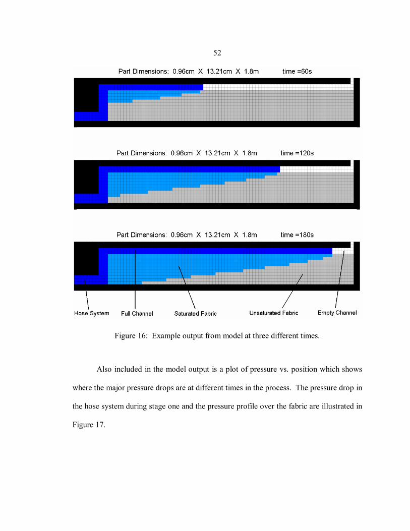
52
Figure 16: Example output from model at three different times.
Also included in the model output is a plot of pressure vs. position which shows
where the major pressure drops are at different times in the process. The pressure drop in
the hose system during stage one and the pressure profile over the fabric are illustrated in
Figure 17.
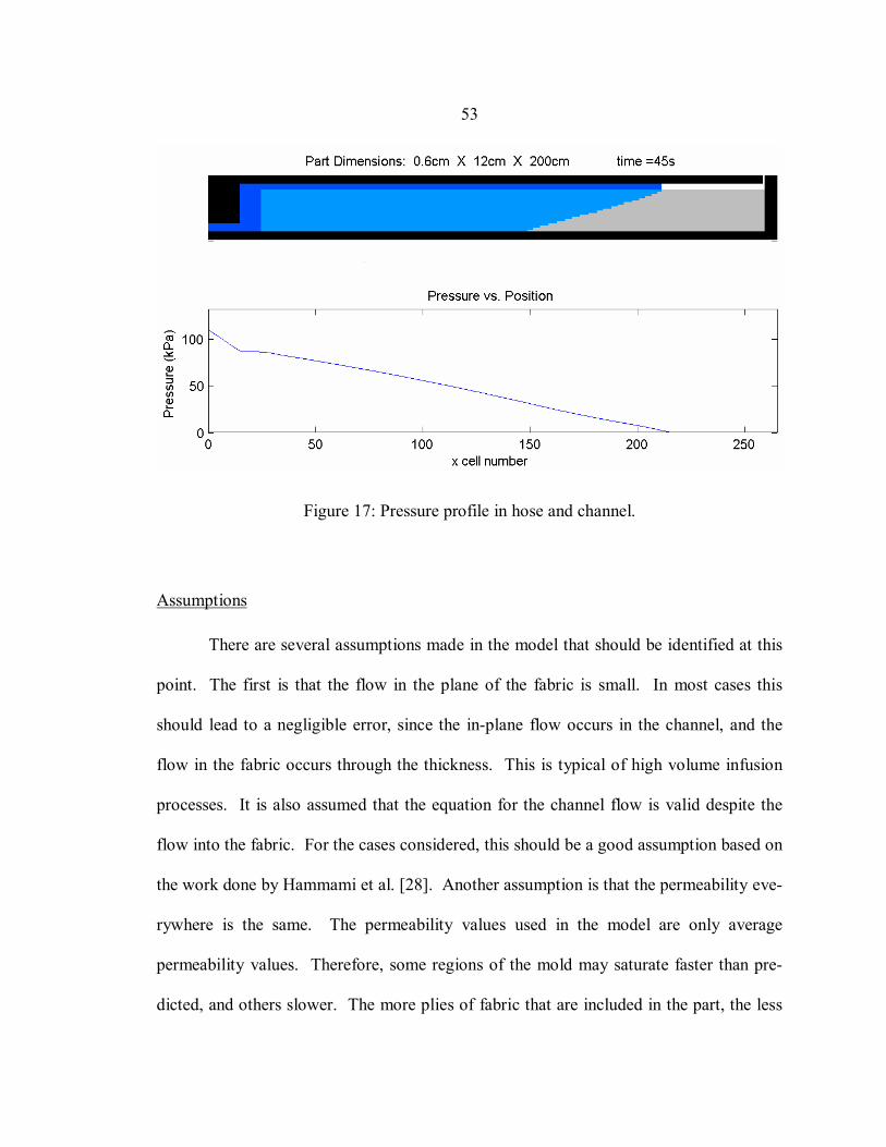
53
Figure 17: Pressure profile in hose and channel.
Assumptions
There are several assumptions made in the model that should be identified at this
point. The first is that the flow in the plane of the fabric is small. In most cases this
should lead to a negligible error, since the in-plane flow occurs in the channel, and the
flow in the fabric occurs through the thickness. This is typical of high volume infusion
processes. It is also assumed that the equation for the channel flow is valid despite the
flow into the fabric. For the cases considered, this should be a good assumption based on
the work done by Hammami et al. [28]. Another assumption is that the permeability eve-
rywhere is the same. The permeability values used in the model are only average
permeability values. Therefore, some regions of the mold may saturate faster than pre-
dicted, and others slower. The more plies of fabric that are included in the part, the less

54
variability. The model also does not account for any fluid flowing around the edges of
the fabric, or “racetracking.” Racetracking could lead to a non-uniform flow front which
could trap air pockets in the part. Because the results of racetracking would be so unde-
sirable, it was assumed that proper precaution would be taken to minimize this effect.
Possibilities for accomplishing this will be discussed later. In some cases, the model uses
average values to represent things that change throughout the process such as the resin
viscosity and pressure.
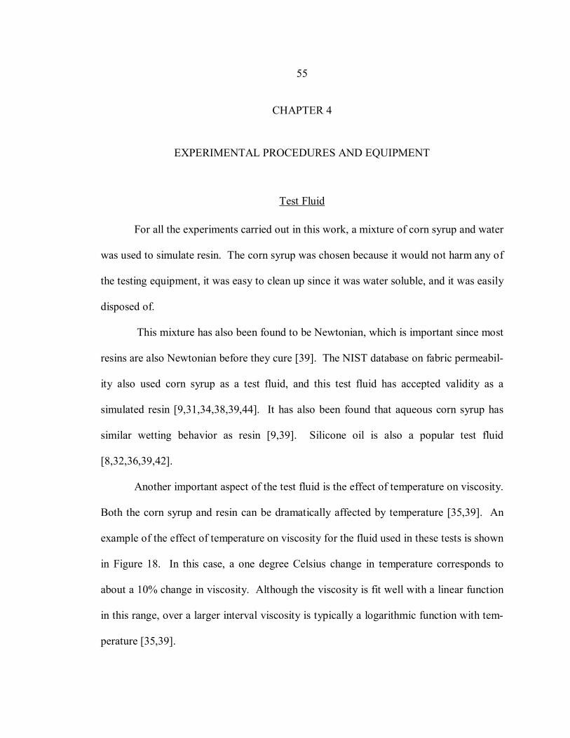
55
CHAPTER 4
EXPERIMENTAL PROCEDURES AND EQUIPMENT
Test Fluid
For all the experiments carried out in this work, a mixture of corn syrup and water
was used to simulate resin. The corn syrup was chosen because it would not harm any of
the testing equipment, it was easy to clean up since it was water soluble, and it was easily
disposed of.
This mixture has also been found to be Newtonian, which is important since most
resins are also Newtonian before they cure [39]. The NIST database on fabric permeabil-
ity also used corn syrup as a test fluid, and this test fluid has accepted validity as a
simulated resin [9,31,34,38,39,44]. It has also been found that aqueous corn syrup has
similar wetting behavior as resin [9,39]. Silicone oil is also a popular test fluid
[8,32,36,39,42].
Another important aspect of the test fluid is the effect of temperature on viscosity.
Both the corn syrup and resin can be dramatically affected by temperature [35,39]. An
example of the effect of temperature on viscosity for the fluid used in these tests is shown
in Figure 18. In this case, a one degree Celsius change in temperature corresponds to
about a 10% change in viscosity. Although the viscosity is fit well with a linear function
in this range, over a larger interval viscosity is typically a logarithmic function with tem-
perature [35,39].
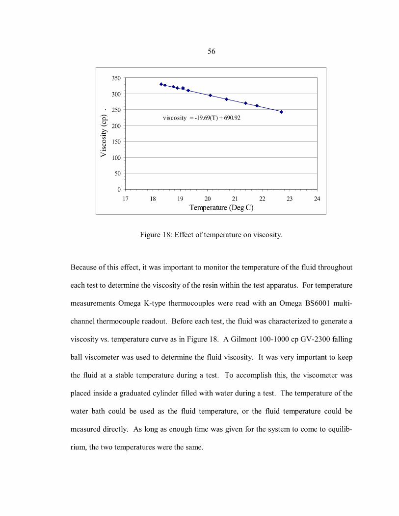
56
viscosity = -19.69(T) + 690.92
0
50
100
150
200
250
300
350
17 18 19 20 21 22 23 24Temperature (Deg C)
Visc
osity
(cp)
.
Figure 18: Effect of temperature on viscosity.
Because of this effect, it was important to monitor the temperature of the fluid throughout
each test to determine the viscosity of the resin within the test apparatus. For temperature
measurements Omega K-type thermocouples were read with an Omega BS6001 multi-
channel thermocouple readout. Before each test, the fluid was characterized to generate a
viscosity vs. temperature curve as in Figure 18. A Gilmont 100-1000 cp GV-2300 falling
ball viscometer was used to determine the fluid viscosity. It was very important to keep
the fluid at a stable temperature during a test. To accomplish this, the viscometer was
placed inside a graduated cylinder filled with water during a test. The temperature of the
water bath could be used as the fluid temperature, or the fluid temperature could be
measured directly. As long as enough time was given for the system to come to equilib-
rium, the two temperatures were the same.
57
By knowing the temperature of the fluid during the test, the corresponding viscos-
ity could be determined and used for calculations. In practice, this strong temperature
dependence could lead to significant error when applying a flow model to a real manufac-
turing process. If the resin or the mold is heated beforehand there could be a large
amount of heat transfer occurring, and large temperature differences throughout the mold.
In this case it would not be accurate to assume a constant viscosity, and may be very dif-
ficult to predict how the viscosity is changing throughout the mold.
One aspect of a resin’s behavior that was not simulated with the corn syrup was
the changing viscosity with time. With a real resin, the viscosity changes constantly with
time due to cross linking and the change in temperature caused by the reaction [45]. This
could have major implications in modeling a real process. Although this effect was not
modeled, it could be done easily by making the viscosity a function of time to match a
given resin.
Injection System Tests
In order to test and validate the flow model created for the injection system a se-
ries of simple tests were performed. A PVC pressure pot was filled with resin and a
constant pressure was applied to the fluid with compressed air. At the outlet of the pres-
sure pot a cross fitting with three outlets and a pressure port was used. The pressure in
the fitting was measured using an Omega 0-35 kPa PX139 pressure transducer. The
transducer was calibrated using an Omega 0-100 kPa type T precision test gauge. This
fitting is shown in Figure 19 and was the basis for the development of equation 3.14.
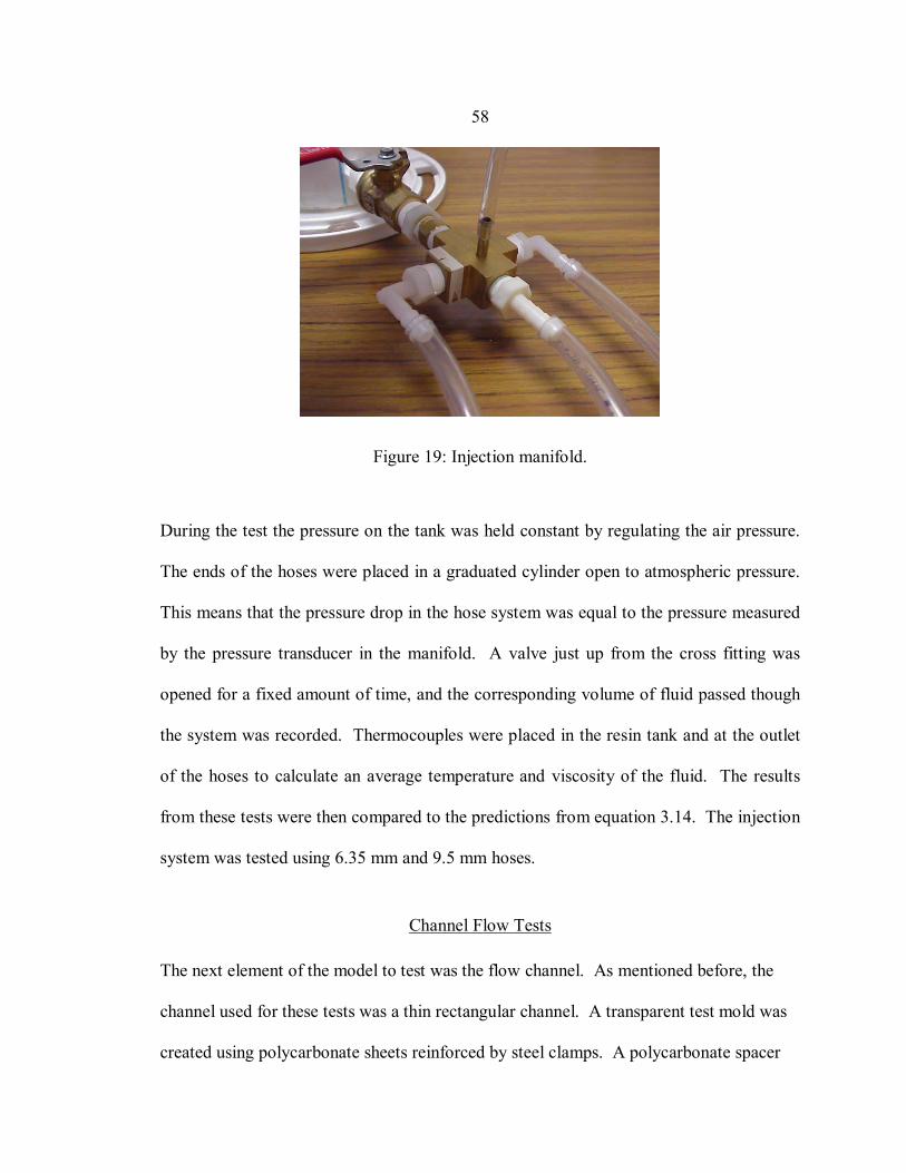
58
Figure 19: Injection manifold.
During the test the pressure on the tank was held constant by regulating the air pressure.
The ends of the hoses were placed in a graduated cylinder open to atmospheric pressure.
This means that the pressure drop in the hose system was equal to the pressure measured
by the pressure transducer in the manifold. A valve just up from the cross fitting was
opened for a fixed amount of time, and the corresponding volume of fluid passed though
the system was recorded. Thermocouples were placed in the resin tank and at the outlet
of the hoses to calculate an average temperature and viscosity of the fluid. The results
from these tests were then compared to the predictions from equation 3.14. The injection
system was tested using 6.35 mm and 9.5 mm hoses.
Channel Flow Tests
The next element of the model to test was the flow channel. As mentioned before, the
channel used for these tests was a thin rectangular channel. A transparent test mold was
created using polycarbonate sheets reinforced by steel clamps. A polycarbonate spacer
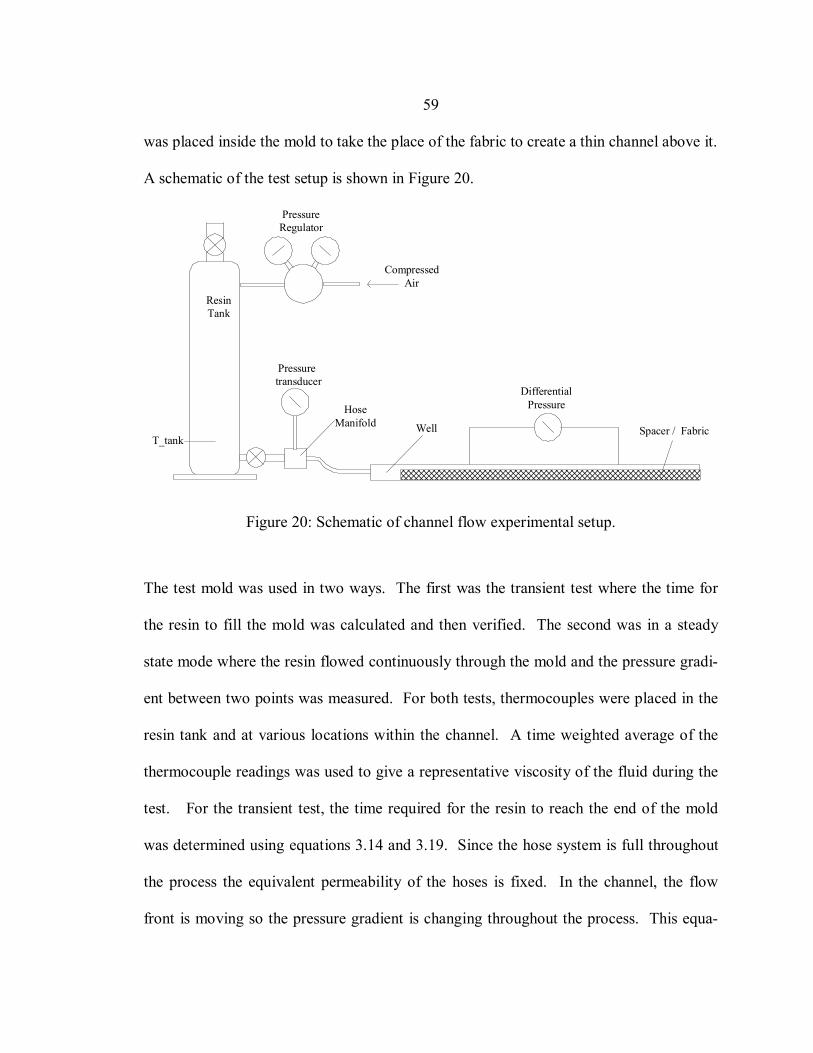
59
was placed inside the mold to take the place of the fabric to create a thin channel above it.
A schematic of the test setup is shown in Figure 20.
T_tank
CompressedAir
PressureRegulator
ResinTank
�������������
HoseManifold Well Spacer / Fabric
DifferentialPressure
Pressure transducer
Figure 20: Schematic of channel flow experimental setup.
The test mold was used in two ways. The first was the transient test where the time for
the resin to fill the mold was calculated and then verified. The second was in a steady
state mode where the resin flowed continuously through the mold and the pressure gradi-
ent between two points was measured. For both tests, thermocouples were placed in the
resin tank and at various locations within the channel. A time weighted average of the
thermocouple readings was used to give a representative viscosity of the fluid during the
test. For the transient test, the time required for the resin to reach the end of the mold
was determined using equations 3.14 and 3.19. Since the hose system is full throughout
the process the equivalent permeability of the hoses is fixed. In the channel, the flow
front is moving so the pressure gradient is changing throughout the process. This equa-
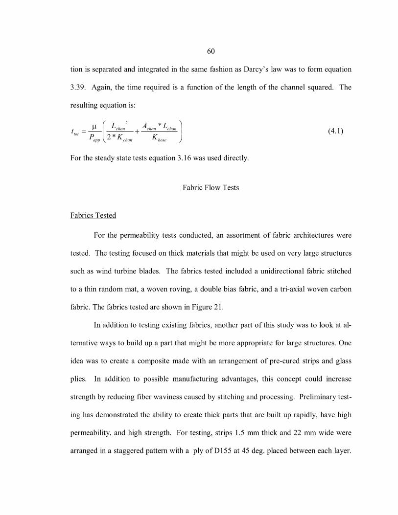
60
tion is separated and integrated in the same fashion as Darcy’s law was to form equation
3.39. Again, the time required is a function of the length of the channel squared. The
resulting equation is:
+=
hose
chanchan
chan
chan
apptot K
LAK
LP
t*
*2
2µ (4.1)
For the steady state tests equation 3.16 was used directly.
Fabric Flow Tests
Fabrics Tested
For the permeability tests conducted, an assortment of fabric architectures were
tested. The testing focused on thick materials that might be used on very large structures
such as wind turbine blades. The fabrics tested included a unidirectional fabric stitched
to a thin random mat, a woven roving, a double bias fabric, and a tri-axial woven carbon
fabric. The fabrics tested are shown in Figure 21.
In addition to testing existing fabrics, another part of this study was to look at al-
ternative ways to build up a part that might be more appropriate for large structures. One
idea was to create a composite made with an arrangement of pre-cured strips and glass
plies. In addition to possible manufacturing advantages, this concept could increase
strength by reducing fiber waviness caused by stitching and processing. Preliminary test-
ing has demonstrated the ability to create thick parts that are built up rapidly, have high
permeability, and high strength. For testing, strips 1.5 mm thick and 22 mm wide were
arranged in a staggered pattern with a ply of D155 at 45 deg. placed between each layer.
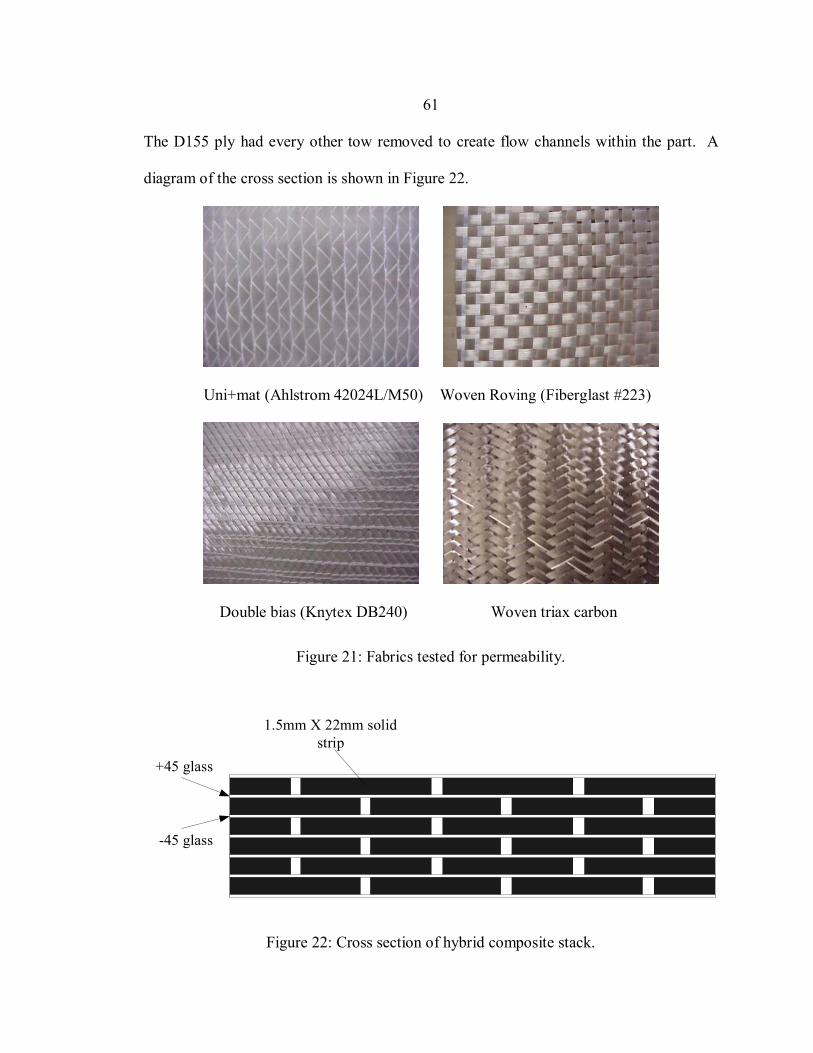
61
The D155 ply had every other tow removed to create flow channels within the part. A
diagram of the cross section is shown in Figure 22.
Uni+mat (Ahlstrom 42024L/M50) Woven Roving (Fiberglast #223)
Double bias (Knytex DB240) Woven triax carbon
Figure 21: Fabrics tested for permeability.
1.5mm X 22mm solidstrip
+45 glass
-45 glass
Figure 22: Cross section of hybrid composite stack.
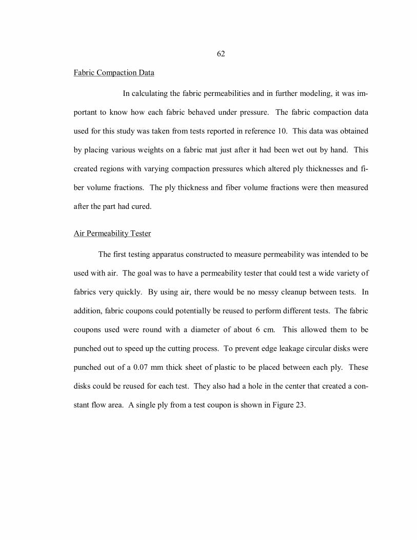
62
Fabric Compaction Data
In calculating the fabric permeabilities and in further modeling, it was im-
portant to know how each fabric behaved under pressure. The fabric compaction data
used for this study was taken from tests reported in reference 10. This data was obtained
by placing various weights on a fabric mat just after it had been wet out by hand. This
created regions with varying compaction pressures which altered ply thicknesses and fi-
ber volume fractions. The ply thickness and fiber volume fractions were then measured
after the part had cured.
Air Permeability Tester
The first testing apparatus constructed to measure permeability was intended to be
used with air. The goal was to have a permeability tester that could test a wide variety of
fabrics very quickly. By using air, there would be no messy cleanup between tests. In
addition, fabric coupons could potentially be reused to perform different tests. The fabric
coupons used were round with a diameter of about 6 cm. This allowed them to be
punched out to speed up the cutting process. To prevent edge leakage circular disks were
punched out of a 0.07 mm thick sheet of plastic to be placed between each ply. These
disks could be reused for each test. They also had a hole in the center that created a con-
stant flow area. A single ply from a test coupon is shown in Figure 23.
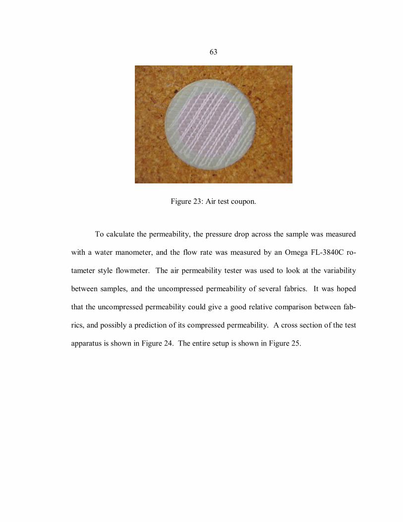
63
Figure 23: Air test coupon.
To calculate the permeability, the pressure drop across the sample was measured
with a water manometer, and the flow rate was measured by an Omega FL-3840C ro-
tameter style flowmeter. The air permeability tester was used to look at the variability
between samples, and the uncompressed permeability of several fabrics. It was hoped
that the uncompressed permeability could give a good relative comparison between fab-
rics, and possibly a prediction of its compressed permeability. A cross section of the test
apparatus is shown in Figure 24. The entire setup is shown in Figure 25.
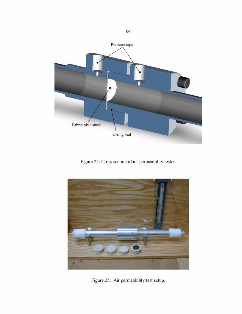
64
Pressure taps
Fabric ply / stack
O-ring seal
Figure 24: Cross section of air permeability tester.
Figure 25: Air permeability test setup.
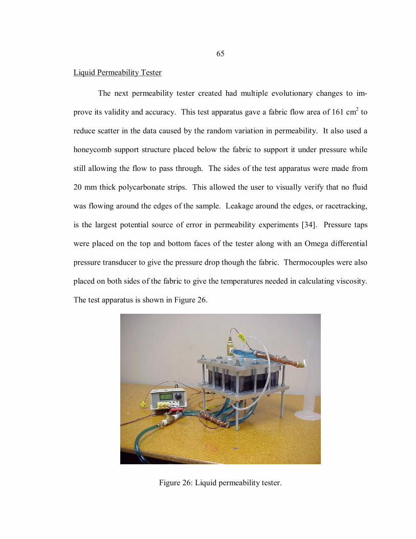
65
Liquid Permeability Tester
The next permeability tester created had multiple evolutionary changes to im-
prove its validity and accuracy. This test apparatus gave a fabric flow area of 161 cm2 to
reduce scatter in the data caused by the random variation in permeability. It also used a
honeycomb support structure placed below the fabric to support it under pressure while
still allowing the flow to pass through. The sides of the test apparatus were made from
20 mm thick polycarbonate strips. This allowed the user to visually verify that no fluid
was flowing around the edges of the sample. Leakage around the edges, or racetracking,
is the largest potential source of error in permeability experiments [34]. Pressure taps
were placed on the top and bottom faces of the tester along with an Omega differential
pressure transducer to give the pressure drop though the fabric. Thermocouples were also
placed on both sides of the fabric to give the temperatures needed in calculating viscosity.
The test apparatus is shown in Figure 26.
Figure 26: Liquid permeability tester.
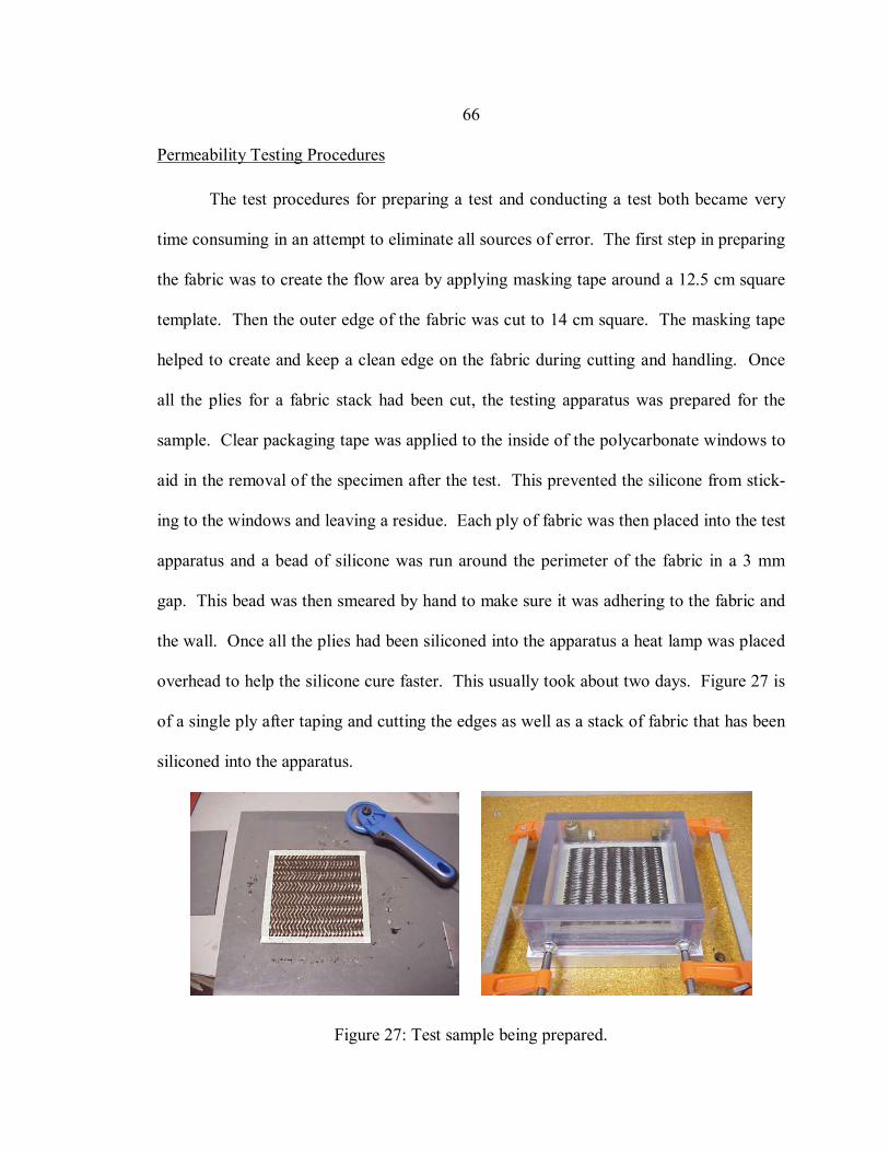
66
Permeability Testing Procedures
The test procedures for preparing a test and conducting a test both became very
time consuming in an attempt to eliminate all sources of error. The first step in preparing
the fabric was to create the flow area by applying masking tape around a 12.5 cm square
template. Then the outer edge of the fabric was cut to 14 cm square. The masking tape
helped to create and keep a clean edge on the fabric during cutting and handling. Once
all the plies for a fabric stack had been cut, the testing apparatus was prepared for the
sample. Clear packaging tape was applied to the inside of the polycarbonate windows to
aid in the removal of the specimen after the test. This prevented the silicone from stick-
ing to the windows and leaving a residue. Each ply of fabric was then placed into the test
apparatus and a bead of silicone was run around the perimeter of the fabric in a 3 mm
gap. This bead was then smeared by hand to make sure it was adhering to the fabric and
the wall. Once all the plies had been siliconed into the apparatus a heat lamp was placed
overhead to help the silicone cure faster. This usually took about two days. Figure 27 is
of a single ply after taping and cutting the edges as well as a stack of fabric that has been
siliconed into the apparatus.
Figure 27: Test sample being prepared.
67
Once the silicone had dried the test apparatus was bolted together. A pressure pot
was used to supply resin to the fabric at a constant supply pressure. It was very important
to slowly fill the test apparatus from the bottom up to avoid creating any bubbles in the
system. The same is true when saturating the fabric. The fabric was saturated from the
bottom up at a low pressure to give the air plenty of time to escape. Trapped air can also
be a significant source of error in permeability testing [34]. Once the system was full, the
fluid was allowed to flow through for a few minutes before a reading was taken. When
going from a lower supply pressure to a higher supply pressure it was very important to
give the fabric time to compress. Because the fabric has a higher porosity at lower pres-
sures it contains more resin. Since these tests are conducted in the saturated state, when a
higher pressure is applied it takes time for the fabric to reject this extra resin as it com-
presses to the next state. Therefore, multiple readings were taken at each point until the
values leveled off. At each point, the differential pressure was recorded throughout the
test with a data logging multi-meter. From this, the average pressure during the test was
determined and used in the calculations. Usually the pressure did not change more than a
few percent during a test. The temperature was also recorded during the test to get the
viscosity. The volumetric flow rate was calculated by measuring the time required to fill
a graduated cylinder to a given volume. From this the velocity was calculated by know-
ing the cross sectional area. The last bit of information required to determine the
permeability was the fabric thickness. As mentioned before, due to compressibility this
value changed at different applied pressures. Unfortunately, measuring the thickness di-
rectly at the different pressures would be very hard to do during the test. To get around
68
this, data from separate compressibility tests were used along with the uncompressed
thickness as recorded before the test. From the compressibility tests a percent reduction
in thickness could be calculated at different pressures and used to calculate the new
thickness. This method of backing out the fabric thickness could lead to some error due
to the fact that the compressibility of a fabric can vary from one stack to the next [34].
However, it could prove just as difficult to measure the thickness of the fabric in-situ with
the current test apparatus.
Another important procedure in the testing was to always work from low pres-
sures to higher pressures. This is because once the fabric has been compressed by a high
pressure it will not spring back to its original state as might be expected, although some
spring back may occur. There are a couple possible explanations for this. One is that it
takes a force to get the fiber tows to mesh with each other, but they are not necessarily in
a strained state once this occurs. Another is the possibility that since the fabric is satu-
rated, for it to spring back it would have to pull resin in to fill the voids created as it
expands. It could be that fabric does not have enough of an elastic force to draw in the
resin in a reasonable amount of time. It may be possible that the fabric would uncom-
press if given enough time, but this could possibly take hours or days. As mentioned
previously, Bickerton et al found that glass fabric could exhibit viscoelastic behavior with
hysteresis [41]. This phenomenon has also been noted by Parnas [34].
Capillary Pressure Tests
A series of tests were performed on the Ahlstrom fabric using the diluted corn
syrup to get an approximate value of the capillary pressure for this fabric and resin pair.
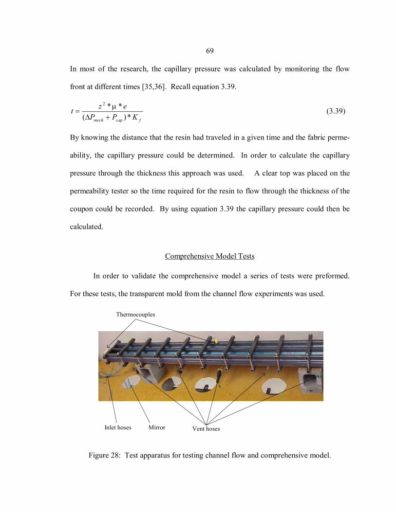
69
In most of the research, the capillary pressure was calculated by monitoring the flow
front at different times [35,36]. Recall equation 3.39.
fcapmech KPPezt*)(
**2
+∆=
µ (3.39)
By knowing the distance that the resin had traveled in a given time and the fabric perme-
ability, the capillary pressure could be determined. In order to calculate the capillary
pressure through the thickness this approach was used. A clear top was placed on the
permeability tester so the time required for the resin to flow through the thickness of the
coupon could be recorded. By using equation 3.39 the capillary pressure could then be
calculated.
Comprehensive Model Tests
In order to validate the comprehensive model a series of tests were preformed.
For these tests, the transparent mold from the channel flow experiments was used.
Vent hosesInlet hoses Mirror
Thermocouples
Figure 28: Test apparatus for testing channel flow and comprehensive model.
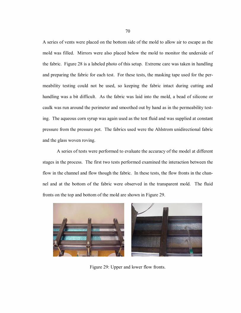
70
A series of vents were placed on the bottom side of the mold to allow air to escape as the
mold was filled. Mirrors were also placed below the mold to monitor the underside of
the fabric. Figure 28 is a labeled photo of this setup. Extreme care was taken in handling
and preparing the fabric for each test. For these tests, the masking tape used for the per-
meability testing could not be used, so keeping the fabric intact during cutting and
handling was a bit difficult. As the fabric was laid into the mold, a bead of silicone or
caulk was run around the perimeter and smoothed out by hand as in the permeability test-
ing. The aqueous corn syrup was again used as the test fluid and was supplied at constant
pressure from the pressure pot. The fabrics used were the Ahlstrom unidirectional fabric
and the glass woven roving.
A series of tests were performed to evaluate the accuracy of the model at different
stages in the process. The first two tests performed examined the interaction between the
flow in the channel and flow though the fabric. In these tests, the flow fronts in the chan-
nel and at the bottom of the fabric were observed in the transparent mold. The fluid
fronts on the top and bottom of the mold are shown in Figure 29.
Figure 29: Upper and lower flow fronts.
71
The next test performed was to examine both stage one and two of the process by
injecting resin until the part was saturated. In the first case, the flexible bagging was not
used to force the resin through the fabric. Instead, the inlet was left open and under pres-
sure so resin was fed in until the part was saturated. The purpose for this was to test the
through thickness stage without the added uncertainty of how the bagging was affecting
the process.
Finally, the process was tested to completion using the flexible bagging for stage
two. In this test, once a given volume of resin had been injected the inlet was closed, and
a pressure was applied to the bagging to force the resin though the thickness. Once the
part was saturated, the inlet was opened to allow any excess resin to exit the mold. An
exit port was also opened on the far end of the mold.
For all the tests, the pressure at the inlet manifold was recorded throughout the
test by a data logging multi-meter. Temperature readings were taken in the tank and at
various points in the test apparatus in order to calculate a representative viscosity.
72
CHAPTER 5
EXPERIMENTAL RESULTS AND ANALYTICAL CORRELATIONS
In this chapter, the results from tests involving the injection system and channel
are compared to the equations derived in the previous chapter. The results from tests
conducted on the various fabric architectures are also presented. The results from these
tests on the individual regions of the process are then used as input to the comprehensive
model. Several experiments are then run to validate the comprehensive model. The re-
sults from the model and experiments are compared at different stages of the process.
The experiments conducted represent processes that are dominated by channel flow and
processes that are dominated by fabric flow.
Injection System Test Results
The predicted results for the injection system compared very well to the experi-
mental results, especially for the smaller hoses. For the 6.35 mm hoses, the predicted
equivalent permeability of the system was 1.36E-4 cm3 and the averaged experimental
value was 1.31E-4 cm3. This results in about a 4% error. For the larger hoses, the pre-
dicted equivalent permeability was 5.18E-4 cm3, and the average experimental value was
4.48E-4 cm3, resulting in a 13% error. One reason why the model was not as accurate for
the larger hoses is that in this case, there is much more pressure drop in the manifold and
hose fittings. The equations used to develop equation 3.14 are most accurate for fully
developed laminar flow. Because of the close proximity of the sharp inlets, exits, and
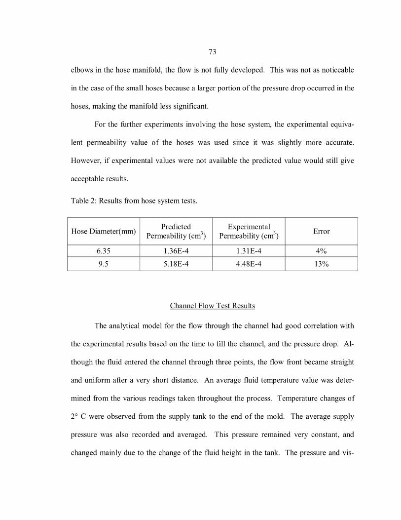
73
elbows in the hose manifold, the flow is not fully developed. This was not as noticeable
in the case of the small hoses because a larger portion of the pressure drop occurred in the
hoses, making the manifold less significant.
For the further experiments involving the hose system, the experimental equiva-
lent permeability value of the hoses was used since it was slightly more accurate.
However, if experimental values were not available the predicted value would still give
acceptable results.
Table 2: Results from hose system tests.
Hose Diameter(mm) Predicted Permeability (cm3)
Experimental Permeability (cm3) Error
6.35 1.36E-4 1.31E-4 4% 9.5 5.18E-4 4.48E-4 13%
Channel Flow Test Results
The analytical model for the flow through the channel had good correlation with
the experimental results based on the time to fill the channel, and the pressure drop. Al-
though the fluid entered the channel through three points, the flow front became straight
and uniform after a very short distance. An average fluid temperature value was deter-
mined from the various readings taken throughout the process. Temperature changes of
2° C were observed from the supply tank to the end of the mold. The average supply
pressure was also recorded and averaged. This pressure remained very constant, and
changed mainly due to the change of the fluid height in the tank. The pressure and vis-
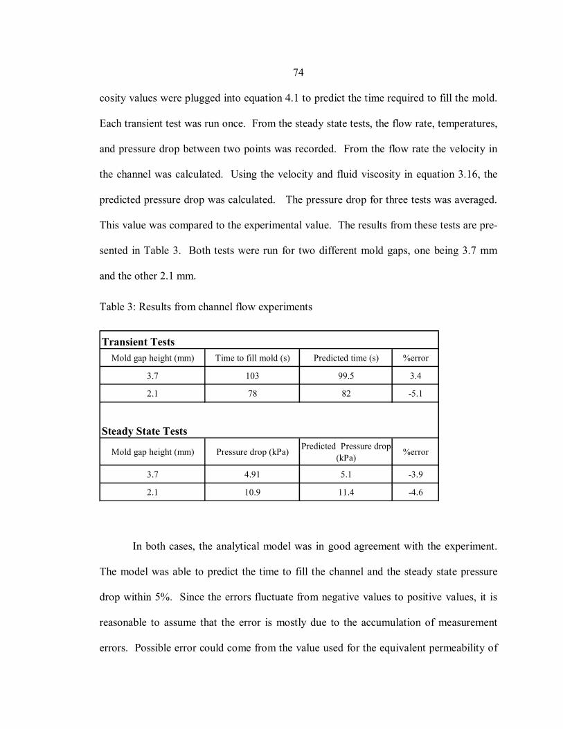
74
cosity values were plugged into equation 4.1 to predict the time required to fill the mold.
Each transient test was run once. From the steady state tests, the flow rate, temperatures,
and pressure drop between two points was recorded. From the flow rate the velocity in
the channel was calculated. Using the velocity and fluid viscosity in equation 3.16, the
predicted pressure drop was calculated. The pressure drop for three tests was averaged.
This value was compared to the experimental value. The results from these tests are pre-
sented in Table 3. Both tests were run for two different mold gaps, one being 3.7 mm
and the other 2.1 mm.
Table 3: Results from channel flow experiments
Transient TestsMold gap height (mm) Time to fill mold (s) Predicted time (s) %error
3.7 103 99.5 3.4
2.1 78 82 -5.1
Steady State Tests
Mold gap height (mm) Pressure drop (kPa) Predicted Pressure drop (kPa)
%error
3.7 4.91 5.1 -3.9
2.1 10.9 11.4 -4.6
In both cases, the analytical model was in good agreement with the experiment.
The model was able to predict the time to fill the channel and the steady state pressure
drop within 5%. Since the errors fluctuate from negative values to positive values, it is
reasonable to assume that the error is mostly due to the accumulation of measurement
errors. Possible error could come from the value used for the equivalent permeability of
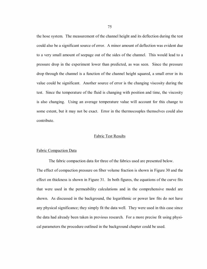
75
the hose system. The measurement of the channel height and its deflection during the test
could also be a significant source of error. A minor amount of deflection was evident due
to a very small amount of seepage out of the sides of the channel. This would lead to a
pressure drop in the experiment lower than predicted, as was seen. Since the pressure
drop through the channel is a function of the channel height squared, a small error in its
value could be significant. Another source of error is the changing viscosity during the
test. Since the temperature of the fluid is changing with position and time, the viscosity
is also changing. Using an average temperature value will account for this change to
some extent, but it may not be exact. Error in the thermocouples themselves could also
contribute.
Fabric Test Results
Fabric Compaction Data
The fabric compaction data for three of the fabrics used are presented below.
The effect of compaction pressure on fiber volume fraction is shown in Figure 30 and the
effect on thickness is shown in Figure 31. In both figures, the equations of the curve fits
that were used in the permeability calculations and in the comprehensive model are
shown. As discussed in the background, the logarithmic or power law fits do not have
any physical significance; they simply fit the data well. They were used in this case since
the data had already been taken in previous research. For a more precise fit using physi-
cal parameters the procedure outlined in the background chapter could be used.
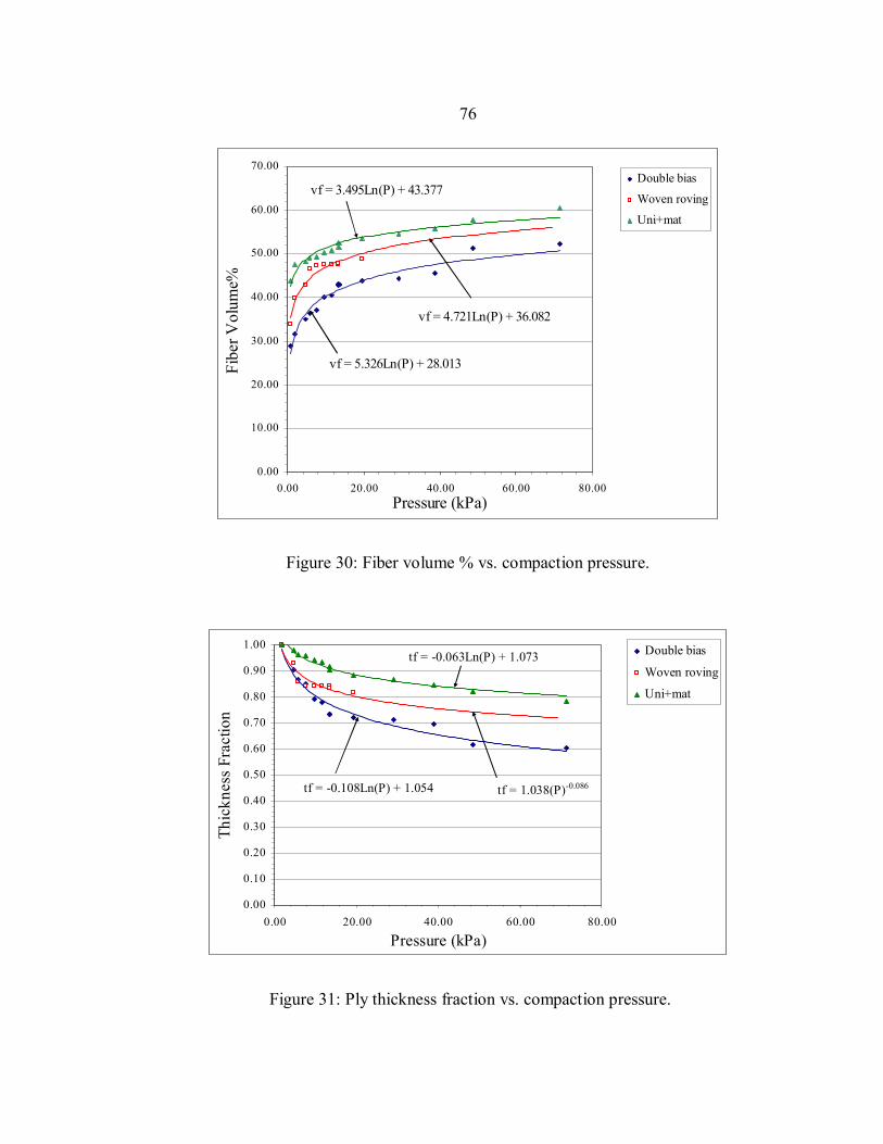
76
vf = 5.326Ln(P) + 28.013
vf = 4.721Ln(P) + 36.082
vf = 3.495Ln(P) + 43.377
0.00
10.00
20.00
30.00
40.00
50.00
60.00
70.00
0.00 20.00 40.00 60.00 80.00Pressure (kPa)
Fibe
r Vol
ume%
Double bias
Woven roving
Uni+mat
Figure 30: Fiber volume % vs. compaction pressure.
tf = -0.108Ln(P) + 1.054 tf = 1.038(P)-0.086
tf = -0.063Ln(P) + 1.073
0.00
0.10
0.20
0.30
0.40
0.50
0.60
0.70
0.80
0.90
1.00
0.00 20.00 40.00 60.00 80.00
Pressure (kPa)
Thic
knes
s Fr
actio
n
Double bias
Woven roving
Uni+mat
Figure 31: Ply thickness fraction vs. compaction pressure.
77
It should also be noted that the ply thickness fractions do not start at 1 for zero pressure.
This is because a very small amount of pressure was applied to the fabric stacks to take a
measurement of the “uncompressed” initial thickness in the permeability tests. Therefore
the initial measurement was not at zero pressure.
The fact that compaction effects diminish at high pressures is illustrated in these
figures. This is because once all the fiber tows are nested and there is glass on glass con-
tact throughout the part, the fabric will behave almost like a solid slab of glass. This is
important in demonstrating that each fabric has a maximum attainable fiber volume frac-
tion. It also demonstrates why the fabric permeability tends to level off at higher
pressures because the fabric becomes fully compressed. It should be noted that there
could be a small amount of error incurred by applying this data to a thick stack since the
tests were performed on lay-ups of two to three plies. According Luce, et al., the com-
pressibility of a fabric can vary depending on the number of plies up to about five plies
[34,46]. After five plies the compressibility is consistent. Based on the results presented
in reference [46], it appears that the difference between two and five plies should be less
than 10%, which is still less than the fabric variability.
Liquid Permeability Test Results
The results from the permeability tests showed a strong relationship between
permeability and compaction pressure. All fabrics had a large decrease in permeability in
the range tested. In all cases, the permeability tended to level off at higher pressures as
the fabric approached its fully compressed state. A plot of the data from the various fab-
rics tested is shown in Figure 32.
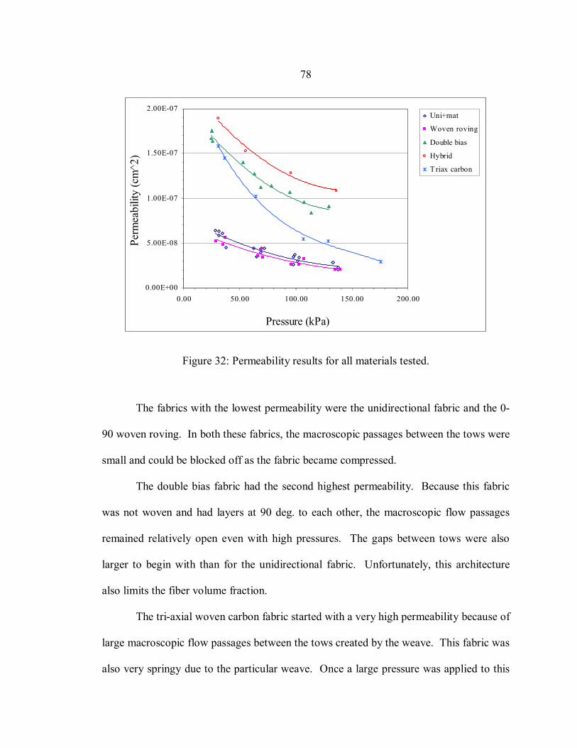
78
0.00E+00
5.00E-08
1.00E-07
1.50E-07
2.00E-07
0.00 50.00 100.00 150.00 200.00
Pressure (kPa)
Perm
eabi
lity
(cm
^2)
Uni+mat
Woven roving
Double bias
Hybrid
Triax carbon
Figure 32: Permeability results for all materials tested.
The fabrics with the lowest permeability were the unidirectional fabric and the 0-
90 woven roving. In both these fabrics, the macroscopic passages between the tows were
small and could be blocked off as the fabric became compressed.
The double bias fabric had the second highest permeability. Because this fabric
was not woven and had layers at 90 deg. to each other, the macroscopic flow passages
remained relatively open even with high pressures. The gaps between tows were also
larger to begin with than for the unidirectional fabric. Unfortunately, this architecture
also limits the fiber volume fraction.
The tri-axial woven carbon fabric started with a very high permeability because of
large macroscopic flow passages between the tows created by the weave. This fabric was
also very springy due to the particular weave. Once a large pressure was applied to this
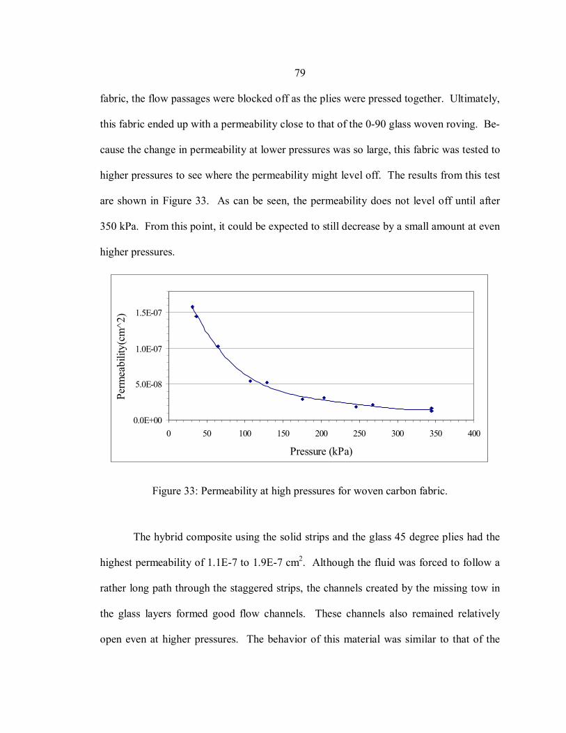
79
fabric, the flow passages were blocked off as the plies were pressed together. Ultimately,
this fabric ended up with a permeability close to that of the 0-90 glass woven roving. Be-
cause the change in permeability at lower pressures was so large, this fabric was tested to
higher pressures to see where the permeability might level off. The results from this test
are shown in Figure 33. As can be seen, the permeability does not level off until after
350 kPa. From this point, it could be expected to still decrease by a small amount at even
higher pressures.
0.0E+00
5.0E-08
1.0E-07
1.5E-07
0 50 100 150 200 250 300 350 400
Pressure (kPa)
Perm
eabi
lity(
cm^2
)
Figure 33: Permeability at high pressures for woven carbon fabric.
The hybrid composite using the solid strips and the glass 45 degree plies had the
highest permeability of 1.1E-7 to 1.9E-7 cm2. Although the fluid was forced to follow a
rather long path through the staggered strips, the channels created by the missing tow in
the glass layers formed good flow channels. These channels also remained relatively
open even at higher pressures. The behavior of this material was similar to that of the
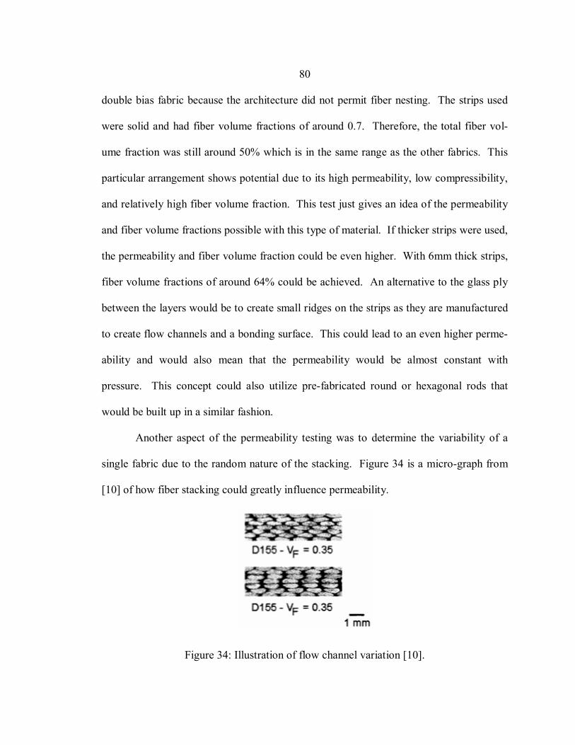
80
double bias fabric because the architecture did not permit fiber nesting. The strips used
were solid and had fiber volume fractions of around 0.7. Therefore, the total fiber vol-
ume fraction was still around 50% which is in the same range as the other fabrics. This
particular arrangement shows potential due to its high permeability, low compressibility,
and relatively high fiber volume fraction. This test just gives an idea of the permeability
and fiber volume fractions possible with this type of material. If thicker strips were used,
the permeability and fiber volume fraction could be even higher. With 6mm thick strips,
fiber volume fractions of around 64% could be achieved. An alternative to the glass ply
between the layers would be to create small ridges on the strips as they are manufactured
to create flow channels and a bonding surface. This could lead to an even higher perme-
ability and would also mean that the permeability would be almost constant with
pressure. This concept could also utilize pre-fabricated round or hexagonal rods that
would be built up in a similar fashion.
Another aspect of the permeability testing was to determine the variability of a
single fabric due to the random nature of the stacking. Figure 34 is a micro-graph from
[10] of how fiber stacking could greatly influence permeability.
Figure 34: Illustration of flow channel variation [10].
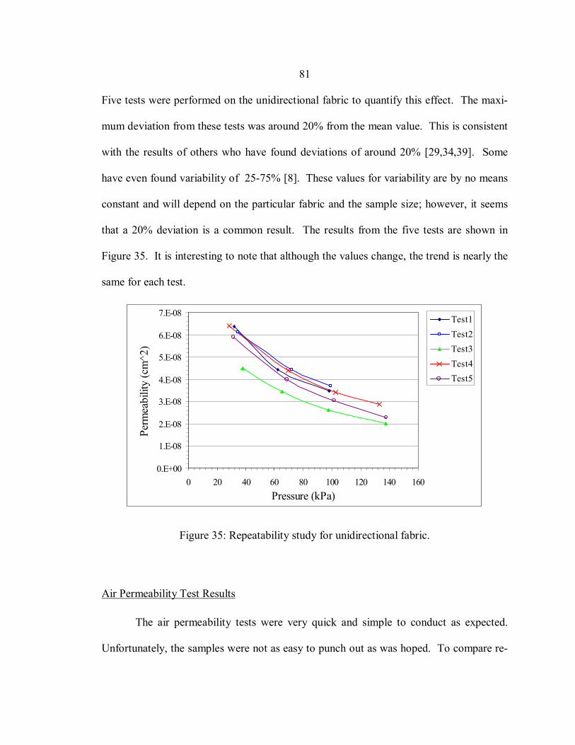
81
Five tests were performed on the unidirectional fabric to quantify this effect. The maxi-
mum deviation from these tests was around 20% from the mean value. This is consistent
with the results of others who have found deviations of around 20% [29,34,39]. Some
have even found variability of 25-75% [8]. These values for variability are by no means
constant and will depend on the particular fabric and the sample size; however, it seems
that a 20% deviation is a common result. The results from the five tests are shown in
Figure 35. It is interesting to note that although the values change, the trend is nearly the
same for each test.
0.E+00
1.E-08
2.E-08
3.E-08
4.E-08
5.E-08
6.E-08
7.E-08
0 20 40 60 80 100 120 140 160Pressure (kPa)
Perm
eabi
lity
(cm
^2)
Test1Test2Test3Test4Test5
Figure 35: Repeatability study for unidirectional fabric.
Air Permeability Test Results
The air permeability tests were very quick and simple to conduct as expected.
Unfortunately, the samples were not as easy to punch out as was hoped. To compare re-
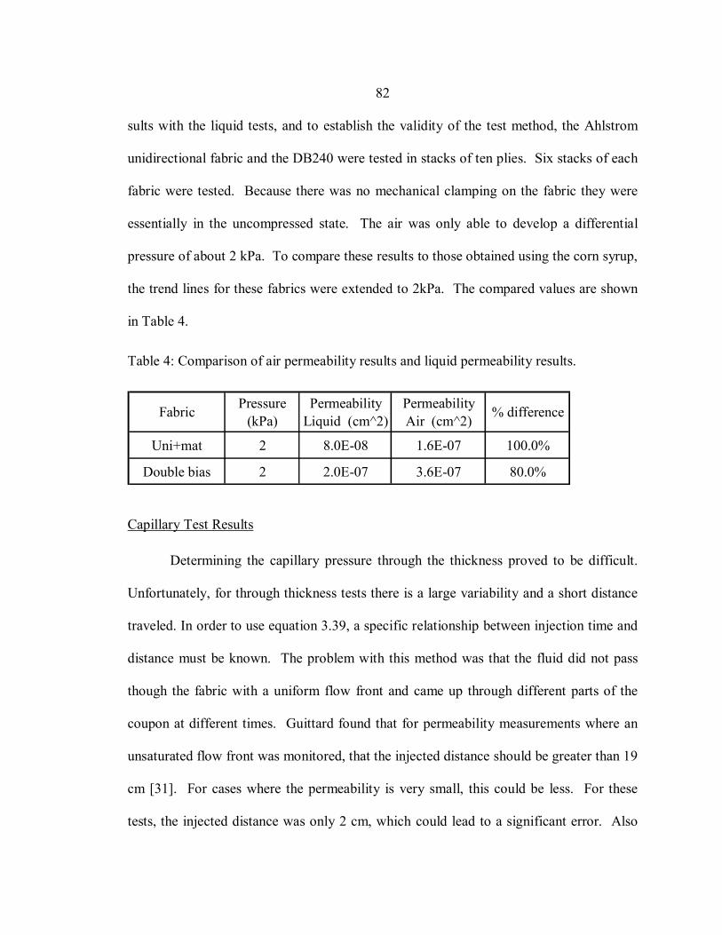
82
sults with the liquid tests, and to establish the validity of the test method, the Ahlstrom
unidirectional fabric and the DB240 were tested in stacks of ten plies. Six stacks of each
fabric were tested. Because there was no mechanical clamping on the fabric they were
essentially in the uncompressed state. The air was only able to develop a differential
pressure of about 2 kPa. To compare these results to those obtained using the corn syrup,
the trend lines for these fabrics were extended to 2kPa. The compared values are shown
in Table 4.
Table 4: Comparison of air permeability results and liquid permeability results.
Fabric Pressure (kPa)
Permeability Liquid (cm^2)
Permeability Air (cm^2) % difference
Uni+mat 2 8.0E-08 1.6E-07 100.0%
Double bias 2 2.0E-07 3.6E-07 80.0%
Capillary Test Results
Determining the capillary pressure through the thickness proved to be difficult.
Unfortunately, for through thickness tests there is a large variability and a short distance
traveled. In order to use equation 3.39, a specific relationship between injection time and
distance must be known. The problem with this method was that the fluid did not pass
though the fabric with a uniform flow front and came up through different parts of the
coupon at different times. Guittard found that for permeability measurements where an
unsaturated flow front was monitored, that the injected distance should be greater than 19
cm [31]. For cases where the permeability is very small, this could be less. For these
tests, the injected distance was only 2 cm, which could lead to a significant error. Also
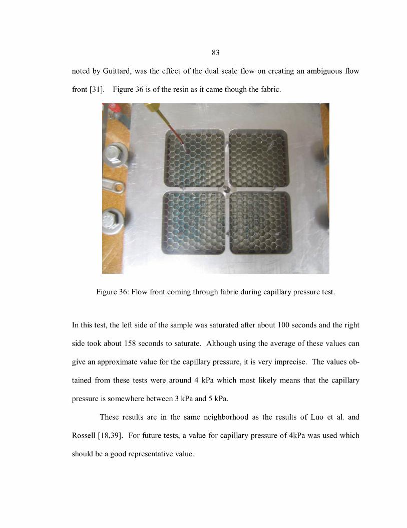
83
noted by Guittard, was the effect of the dual scale flow on creating an ambiguous flow
front [31]. Figure 36 is of the resin as it came though the fabric.
Figure 36: Flow front coming through fabric during capillary pressure test.
In this test, the left side of the sample was saturated after about 100 seconds and the right
side took about 158 seconds to saturate. Although using the average of these values can
give an approximate value for the capillary pressure, it is very imprecise. The values ob-
tained from these tests were around 4 kPa which most likely means that the capillary
pressure is somewhere between 3 kPa and 5 kPa.
These results are in the same neighborhood as the results of Luo et al. and
Rossell [18,39]. For future tests, a value for capillary pressure of 4kPa was used which
should be a good representative value.
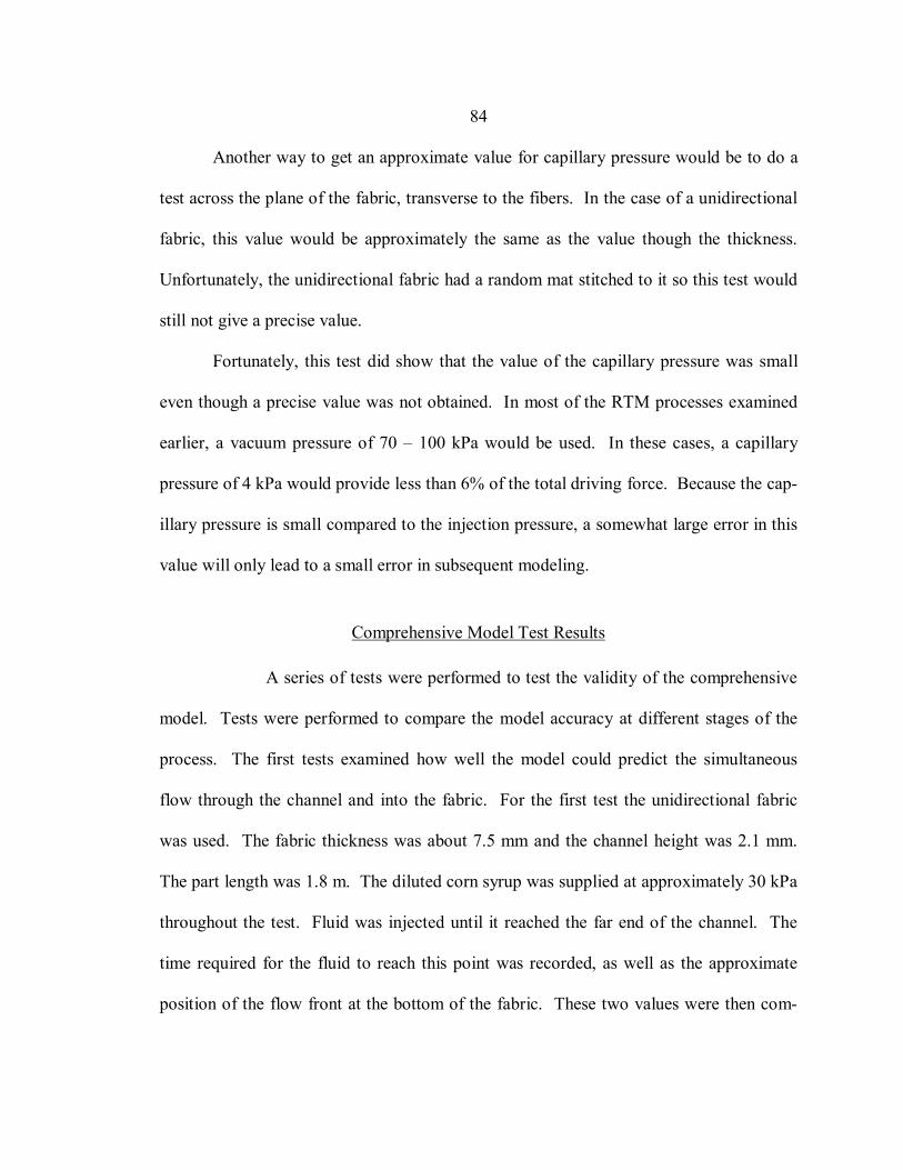
84
Another way to get an approximate value for capillary pressure would be to do a
test across the plane of the fabric, transverse to the fibers. In the case of a unidirectional
fabric, this value would be approximately the same as the value though the thickness.
Unfortunately, the unidirectional fabric had a random mat stitched to it so this test would
still not give a precise value.
Fortunately, this test did show that the value of the capillary pressure was small
even though a precise value was not obtained. In most of the RTM processes examined
earlier, a vacuum pressure of 70 – 100 kPa would be used. In these cases, a capillary
pressure of 4 kPa would provide less than 6% of the total driving force. Because the cap-
illary pressure is small compared to the injection pressure, a somewhat large error in this
value will only lead to a small error in subsequent modeling.
Comprehensive Model Test Results
A series of tests were performed to test the validity of the comprehensive
model. Tests were performed to compare the model accuracy at different stages of the
process. The first tests examined how well the model could predict the simultaneous
flow through the channel and into the fabric. For the first test the unidirectional fabric
was used. The fabric thickness was about 7.5 mm and the channel height was 2.1 mm.
The part length was 1.8 m. The diluted corn syrup was supplied at approximately 30 kPa
throughout the test. Fluid was injected until it reached the far end of the channel. The
time required for the fluid to reach this point was recorded, as well as the approximate
position of the flow front at the bottom of the fabric. These two values were then com-
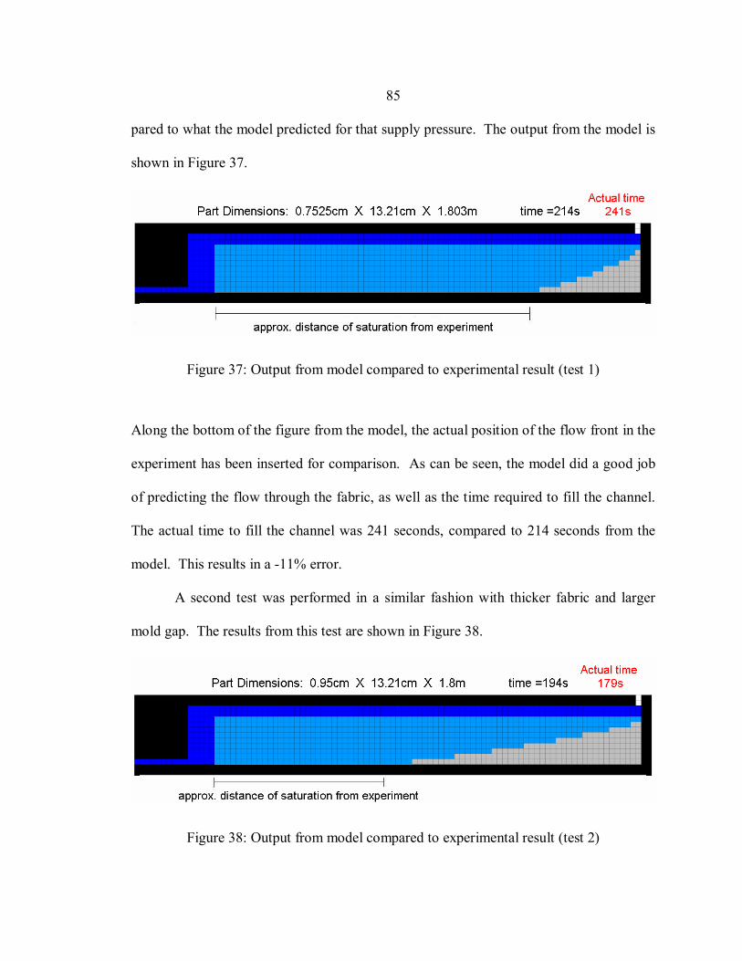
85
pared to what the model predicted for that supply pressure. The output from the model is
shown in Figure 37.
Figure 37: Output from model compared to experimental result (test 1)
Along the bottom of the figure from the model, the actual position of the flow front in the
experiment has been inserted for comparison. As can be seen, the model did a good job
of predicting the flow through the fabric, as well as the time required to fill the channel.
The actual time to fill the channel was 241 seconds, compared to 214 seconds from the
model. This results in a -11% error.
A second test was performed in a similar fashion with thicker fabric and larger
mold gap. The results from this test are shown in Figure 38.
Figure 38: Output from model compared to experimental result (test 2)
86
For this second case the time prediction was closer to the experiment, and the model still
did a good job of predicting the flow front. The actual time required to reach the end of
the mold was 179 seconds, while the predicted time was 194 seconds. This results in an
8% error in the time prediction.
The next stage of the testing was to test the model accuracy after the fluid had
reached the end of the mold. To get a better idea of how the model would perform for the
through-thickness step, the fabric thickness was increased to about 2 cm. The first ex-
periment was run without the use of the flexible bagging to isolate its effect. The resin
was forced through the thickness by keeping the inlet open and continuously feeding in
resin until the part was saturated. The total time required to saturate the part was re-
corded to compare to the predicted value. The supply pressure recorded during the test
was duplicated in the model. It was difficult to judge when the entire sample was satu-
rated. This made precise comparisons between the model and the experiment difficult.
The clear plate on the bottom made it easy to see the resin coming through, but it was
hard to pick an exact saturation time. For example, there was about a twenty second in-
terval from when the part appeared to be about 98% saturated to when it was completely
saturated. Because of this, the saturation time in the experiment will be presented as a
range. For the third test, the saturation time was within 196 – 211 seconds. The model
predicted a saturation time of 208 seconds, which was right in the experimental range.
The final experiment added the additional effect of the bagging film. In this case,
a given amount of resin was injected and then the inlet was closed. Pressure was then
applied to the bagging to force the resin though the thickness. Again, an interval of time
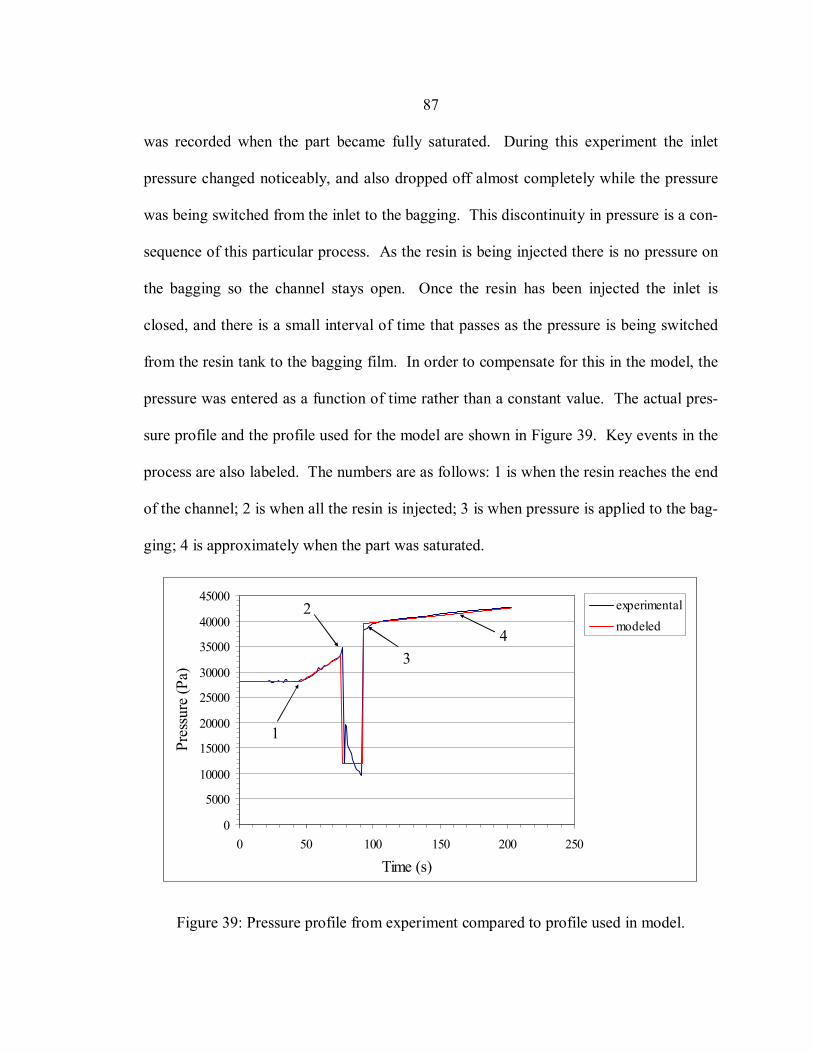
87
was recorded when the part became fully saturated. During this experiment the inlet
pressure changed noticeably, and also dropped off almost completely while the pressure
was being switched from the inlet to the bagging. This discontinuity in pressure is a con-
sequence of this particular process. As the resin is being injected there is no pressure on
the bagging so the channel stays open. Once the resin has been injected the inlet is
closed, and there is a small interval of time that passes as the pressure is being switched
from the resin tank to the bagging film. In order to compensate for this in the model, the
pressure was entered as a function of time rather than a constant value. The actual pres-
sure profile and the profile used for the model are shown in Figure 39. Key events in the
process are also labeled. The numbers are as follows: 1 is when the resin reaches the end
of the channel; 2 is when all the resin is injected; 3 is when pressure is applied to the bag-
ging; 4 is approximately when the part was saturated.
0
5000
10000
15000
20000
25000
30000
35000
40000
45000
0 50 100 150 200 250
Time (s)
Pres
sure
(Pa)
experimentalmodeled
1
2
34
Figure 39: Pressure profile from experiment compared to profile used in model.
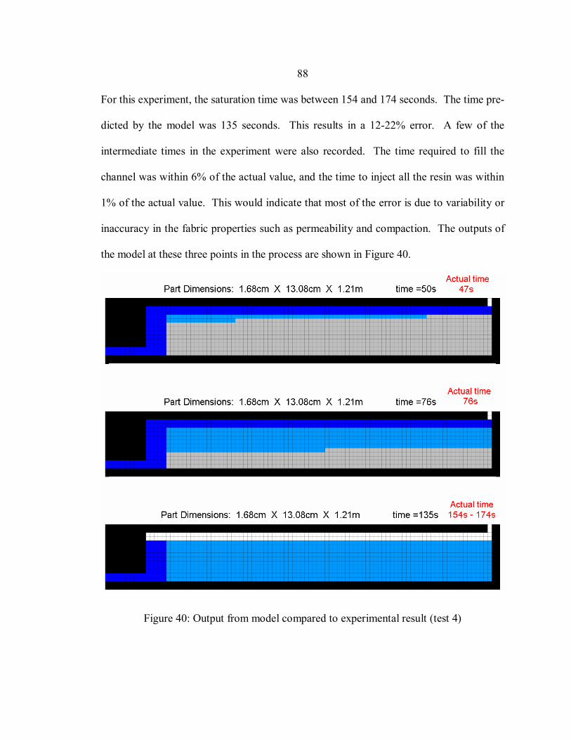
88
For this experiment, the saturation time was between 154 and 174 seconds. The time pre-
dicted by the model was 135 seconds. This results in a 12-22% error. A few of the
intermediate times in the experiment were also recorded. The time required to fill the
channel was within 6% of the actual value, and the time to inject all the resin was within
1% of the actual value. This would indicate that most of the error is due to variability or
inaccuracy in the fabric properties such as permeability and compaction. The outputs of
the model at these three points in the process are shown in Figure 40.
Figure 40: Output from model compared to experimental result (test 4)

89
In order to ensure that the part was saturated, slightly more resin than was needed
was injected. In order to eject this extra resin, the inlet port was reopened after the part
was saturated to allow it to escape. There was also a similar port on the opposite end of
the mold to let the resin out. Once the part was saturated there was essentially zero flow
coming out of the vents at the bottom. This is because the resin would have to flow over
large distances through the thickness and in the plane of the fabric to reach one of these
vents. This is why the vent ports were included above the fabric and would be critical to
any process of this type. This part of the process was not included in the model, but as
long as the amount of extra resin is small, it should be minor. A peel ply could also be
used to strip any extra resin off the top of the part.
The fabric samples used in the last two tests were also examined for any air pock-
ets or dry spots. The layers of fabric were peeled away and examined. No dry spots were
detected during this process.
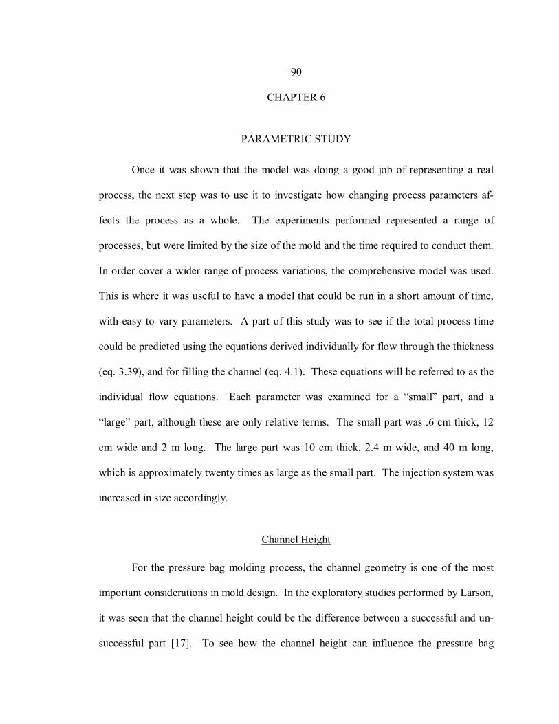
90
CHAPTER 6
PARAMETRIC STUDY
Once it was shown that the model was doing a good job of representing a real
process, the next step was to use it to investigate how changing process parameters af-
fects the process as a whole. The experiments performed represented a range of
processes, but were limited by the size of the mold and the time required to conduct them.
In order cover a wider range of process variations, the comprehensive model was used.
This is where it was useful to have a model that could be run in a short amount of time,
with easy to vary parameters. A part of this study was to see if the total process time
could be predicted using the equations derived individually for flow through the thickness
(eq. 3.39), and for filling the channel (eq. 4.1). These equations will be referred to as the
individual flow equations. Each parameter was examined for a “small” part, and a
“large” part, although these are only relative terms. The small part was .6 cm thick, 12
cm wide and 2 m long. The large part was 10 cm thick, 2.4 m wide, and 40 m long,
which is approximately twenty times as large as the small part. The injection system was
increased in size accordingly.
Channel Height
For the pressure bag molding process, the channel geometry is one of the most
important considerations in mold design. In the exploratory studies performed by Larson,
it was seen that the channel height could be the difference between a successful and un-
successful part [17]. To see how the channel height can influence the pressure bag
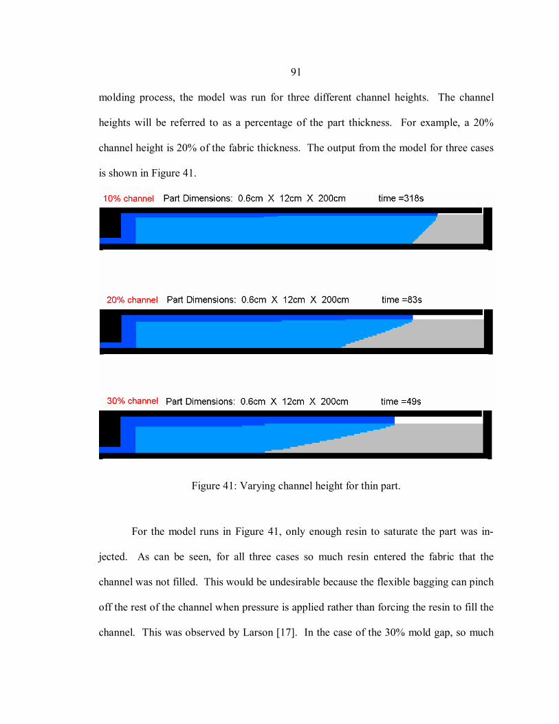
91
molding process, the model was run for three different channel heights. The channel
heights will be referred to as a percentage of the part thickness. For example, a 20%
channel height is 20% of the fabric thickness. The output from the model for three cases
is shown in Figure 41.
Figure 41: Varying channel height for thin part.
For the model runs in Figure 41, only enough resin to saturate the part was in-
jected. As can be seen, for all three cases so much resin entered the fabric that the
channel was not filled. This would be undesirable because the flexible bagging can pinch
off the rest of the channel when pressure is applied rather than forcing the resin to fill the
channel. This was observed by Larson [17]. In the case of the 30% mold gap, so much
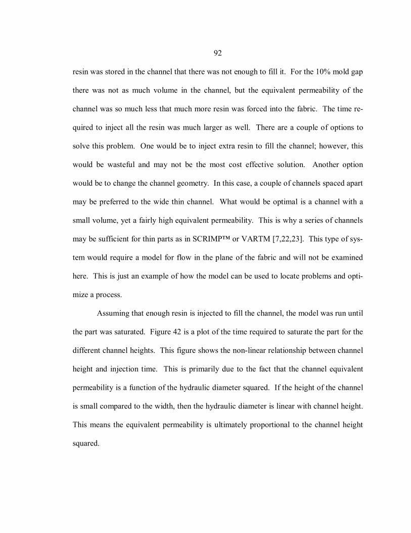
92
resin was stored in the channel that there was not enough to fill it. For the 10% mold gap
there was not as much volume in the channel, but the equivalent permeability of the
channel was so much less that much more resin was forced into the fabric. The time re-
quired to inject all the resin was much larger as well. There are a couple of options to
solve this problem. One would be to inject extra resin to fill the channel; however, this
would be wasteful and may not be the most cost effective solution. Another option
would be to change the channel geometry. In this case, a couple of channels spaced apart
may be preferred to the wide thin channel. What would be optimal is a channel with a
small volume, yet a fairly high equivalent permeability. This is why a series of channels
may be sufficient for thin parts as in SCRIMP™ or VARTM [7,22,23]. This type of sys-
tem would require a model for flow in the plane of the fabric and will not be examined
here. This is just an example of how the model can be used to locate problems and opti-
mize a process.
Assuming that enough resin is injected to fill the channel, the model was run until
the part was saturated. Figure 42 is a plot of the time required to saturate the part for the
different channel heights. This figure shows the non-linear relationship between channel
height and injection time. This is primarily due to the fact that the channel equivalent
permeability is a function of the hydraulic diameter squared. If the height of the channel
is small compared to the width, then the hydraulic diameter is linear with channel height.
This means the equivalent permeability is ultimately proportional to the channel height
squared.
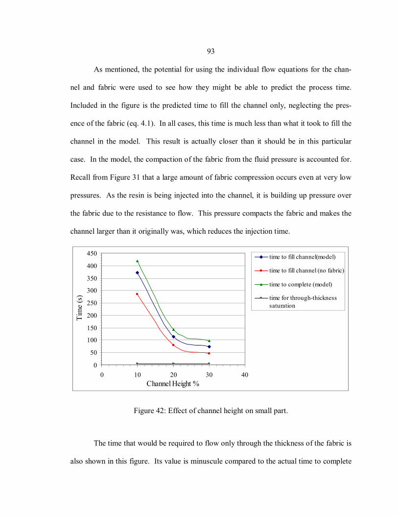
93
As mentioned, the potential for using the individual flow equations for the chan-
nel and fabric were used to see how they might be able to predict the process time.
Included in the figure is the predicted time to fill the channel only, neglecting the pres-
ence of the fabric (eq. 4.1). In all cases, this time is much less than what it took to fill the
channel in the model. This result is actually closer than it should be in this particular
case. In the model, the compaction of the fabric from the fluid pressure is accounted for.
Recall from Figure 31 that a large amount of fabric compression occurs even at very low
pressures. As the resin is being injected into the channel, it is building up pressure over
the fabric due to the resistance to flow. This pressure compacts the fabric and makes the
channel larger than it originally was, which reduces the injection time.
0
50
100
150
200
250
300
350
400
450
0 10 20 30 40Channel Height %
Tim
e (s
)
time to fill channel(model)
time to fill channel (no fabric)
time to complete (model)
time for through-thicknesssaturation
Figure 42: Effect of channel height on small part.
The time that would be required to flow only through the thickness of the fabric is
also shown in this figure. Its value is minuscule compared to the actual time to complete
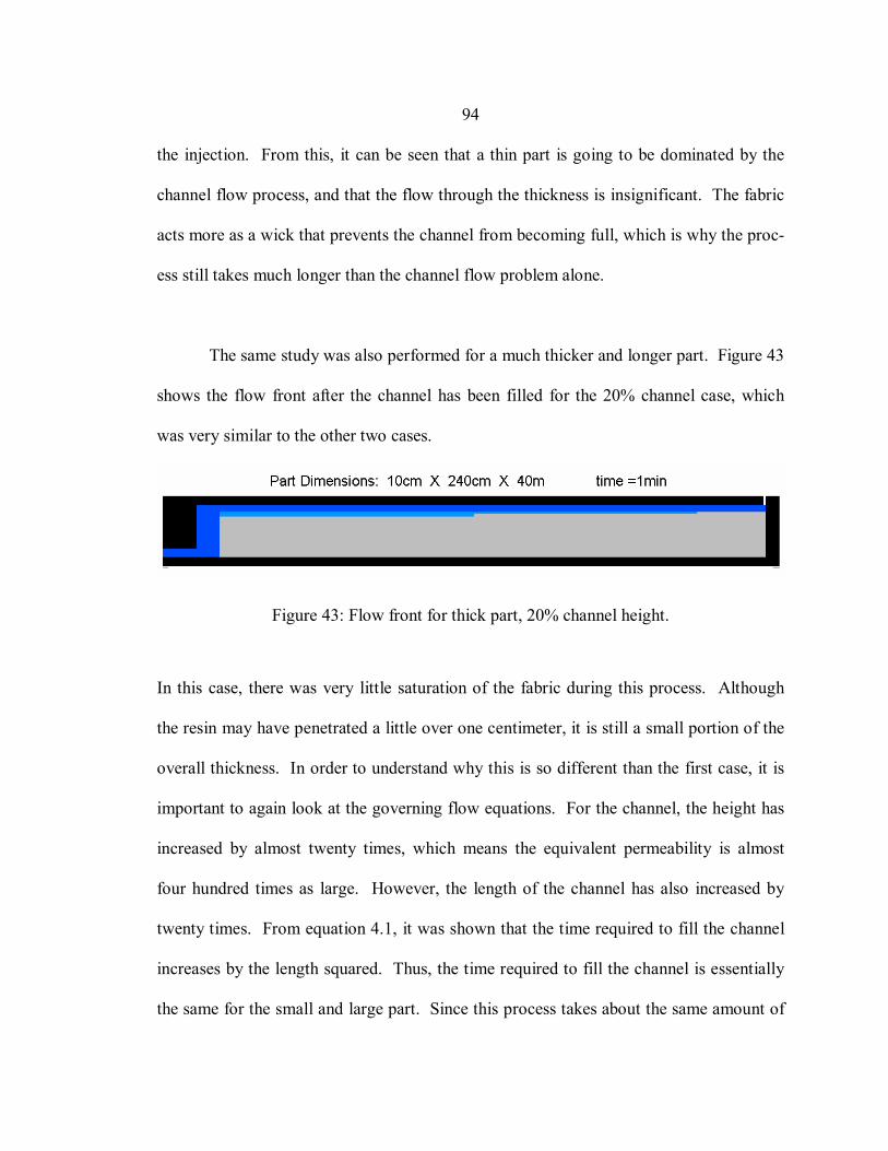
94
the injection. From this, it can be seen that a thin part is going to be dominated by the
channel flow process, and that the flow through the thickness is insignificant. The fabric
acts more as a wick that prevents the channel from becoming full, which is why the proc-
ess still takes much longer than the channel flow problem alone.
The same study was also performed for a much thicker and longer part. Figure 43
shows the flow front after the channel has been filled for the 20% channel case, which
was very similar to the other two cases.
Figure 43: Flow front for thick part, 20% channel height.
In this case, there was very little saturation of the fabric during this process. Although
the resin may have penetrated a little over one centimeter, it is still a small portion of the
overall thickness. In order to understand why this is so different than the first case, it is
important to again look at the governing flow equations. For the channel, the height has
increased by almost twenty times, which means the equivalent permeability is almost
four hundred times as large. However, the length of the channel has also increased by
twenty times. From equation 4.1, it was shown that the time required to fill the channel
increases by the length squared. Thus, the time required to fill the channel is essentially
the same for the small and large part. Since this process takes about the same amount of
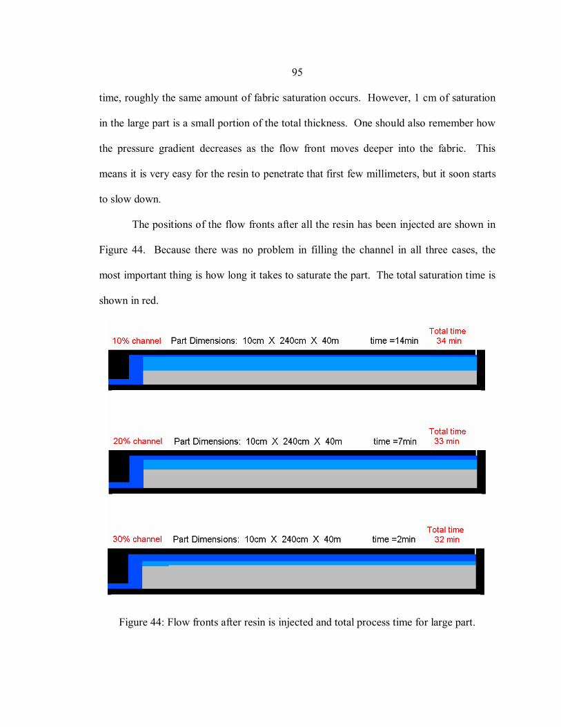
95
time, roughly the same amount of fabric saturation occurs. However, 1 cm of saturation
in the large part is a small portion of the total thickness. One should also remember how
the pressure gradient decreases as the flow front moves deeper into the fabric. This
means it is very easy for the resin to penetrate that first few millimeters, but it soon starts
to slow down.
The positions of the flow fronts after all the resin has been injected are shown in
Figure 44. Because there was no problem in filling the channel in all three cases, the
most important thing is how long it takes to saturate the part. The total saturation time is
shown in red.
Figure 44: Flow fronts after resin is injected and total process time for large part.
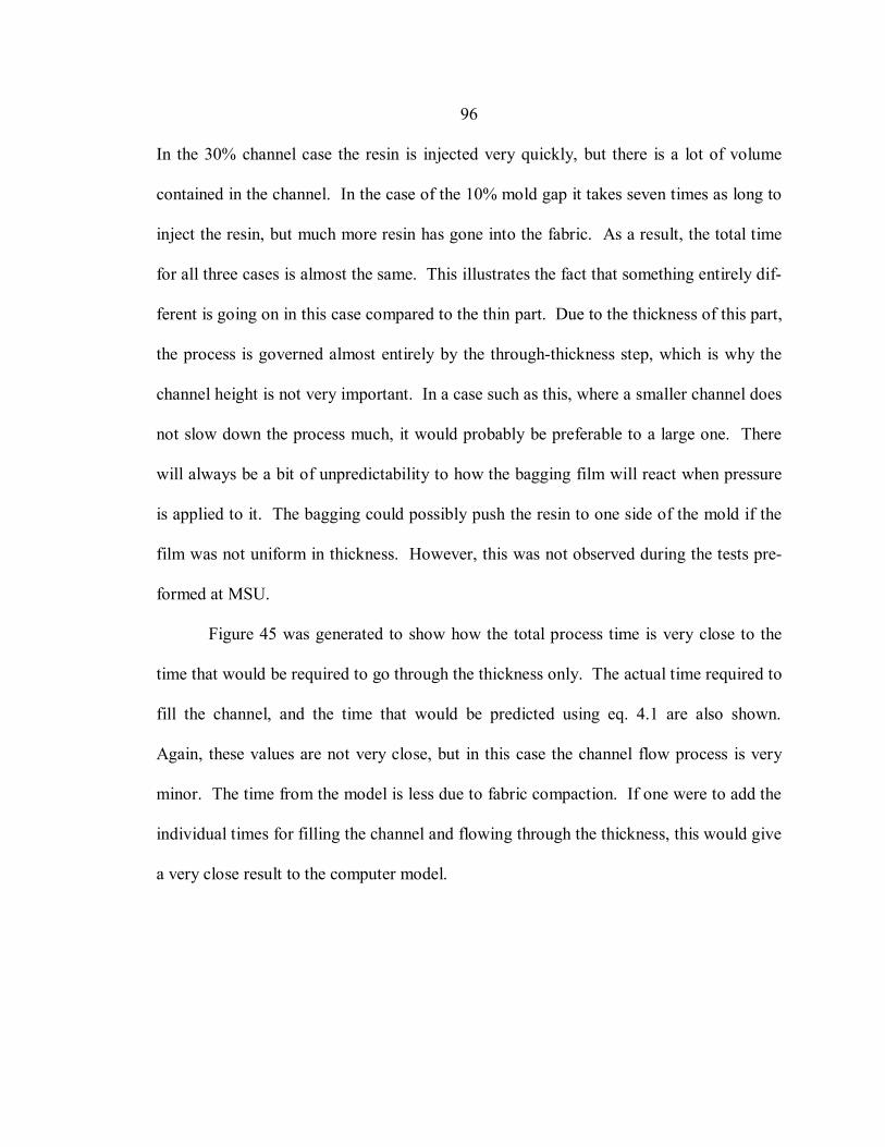
96
In the 30% channel case the resin is injected very quickly, but there is a lot of volume
contained in the channel. In the case of the 10% mold gap it takes seven times as long to
inject the resin, but much more resin has gone into the fabric. As a result, the total time
for all three cases is almost the same. This illustrates the fact that something entirely dif-
ferent is going on in this case compared to the thin part. Due to the thickness of this part,
the process is governed almost entirely by the through-thickness step, which is why the
channel height is not very important. In a case such as this, where a smaller channel does
not slow down the process much, it would probably be preferable to a large one. There
will always be a bit of unpredictability to how the bagging film will react when pressure
is applied to it. The bagging could possibly push the resin to one side of the mold if the
film was not uniform in thickness. However, this was not observed during the tests pre-
formed at MSU.
Figure 45 was generated to show how the total process time is very close to the
time that would be required to go through the thickness only. The actual time required to
fill the channel, and the time that would be predicted using eq. 4.1 are also shown.
Again, these values are not very close, but in this case the channel flow process is very
minor. The time from the model is less due to fabric compaction. If one were to add the
individual times for filling the channel and flowing through the thickness, this would give
a very close result to the computer model.
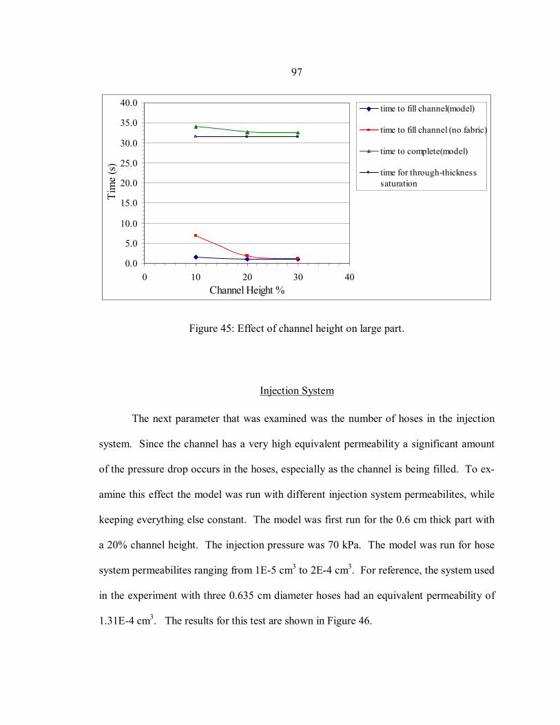
97
0.0
5.0
10.0
15.0
20.0
25.0
30.0
35.0
40.0
0 10 20 30 40Channel Height %
Tim
e (s
)time to fill channel(model)
time to fill channel (no fabric)
time to complete(model)
time for through-thicknesssaturation
Figure 45: Effect of channel height on large part.
Injection System
The next parameter that was examined was the number of hoses in the injection
system. Since the channel has a very high equivalent permeability a significant amount
of the pressure drop occurs in the hoses, especially as the channel is being filled. To ex-
amine this effect the model was run with different injection system permeabilites, while
keeping everything else constant. The model was first run for the 0.6 cm thick part with
a 20% channel height. The injection pressure was 70 kPa. The model was run for hose
system permeabilites ranging from 1E-5 cm3 to 2E-4 cm3. For reference, the system used
in the experiment with three 0.635 cm diameter hoses had an equivalent permeability of
1.31E-4 cm3. The results for this test are shown in Figure 46.
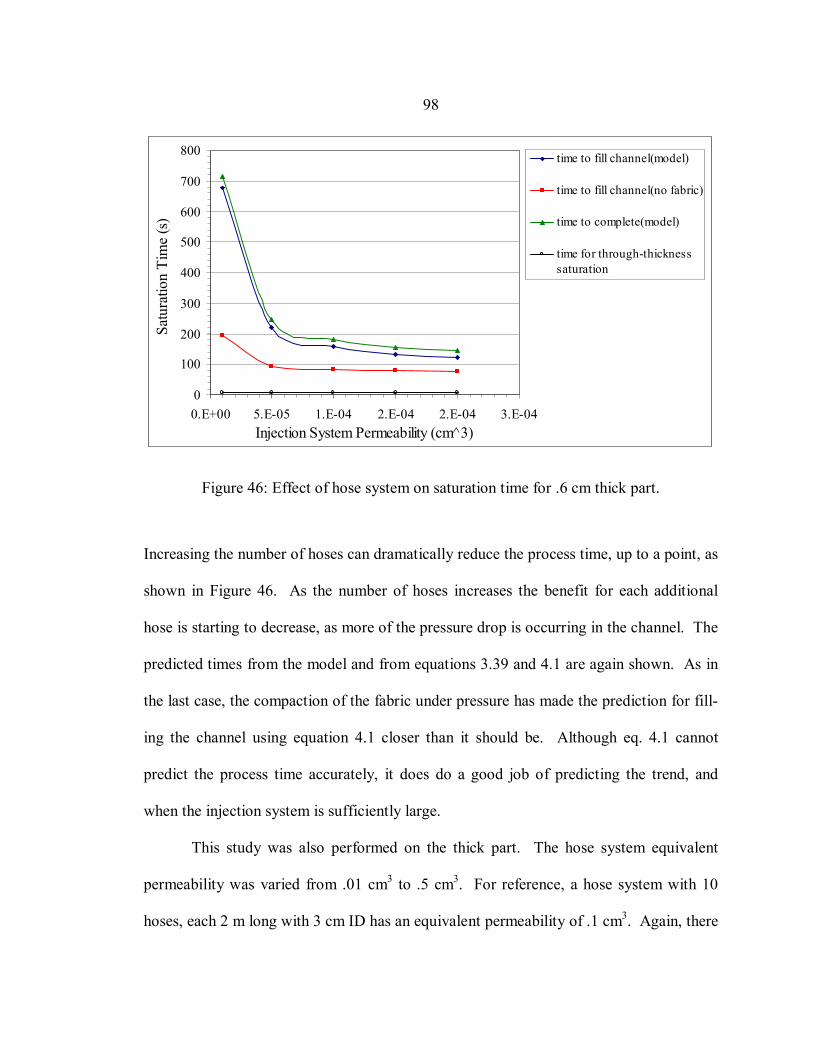
98
0
100
200
300
400
500
600
700
800
0.E+00 5.E-05 1.E-04 2.E-04 2.E-04 3.E-04Injection System Permeability (cm^3)
Satu
ratio
n Ti
me
(s)
time to fill channel(model)
time to fill channel(no fabric)
time to complete(model)
time for through-thicknesssaturation
Figure 46: Effect of hose system on saturation time for .6 cm thick part.
Increasing the number of hoses can dramatically reduce the process time, up to a point, as
shown in Figure 46. As the number of hoses increases the benefit for each additional
hose is starting to decrease, as more of the pressure drop is occurring in the channel. The
predicted times from the model and from equations 3.39 and 4.1 are again shown. As in
the last case, the compaction of the fabric under pressure has made the prediction for fill-
ing the channel using equation 4.1 closer than it should be. Although eq. 4.1 cannot
predict the process time accurately, it does do a good job of predicting the trend, and
when the injection system is sufficiently large.
This study was also performed on the thick part. The hose system equivalent
permeability was varied from .01 cm3 to .5 cm3. For reference, a hose system with 10
hoses, each 2 m long with 3 cm ID has an equivalent permeability of .1 cm3. Again, there
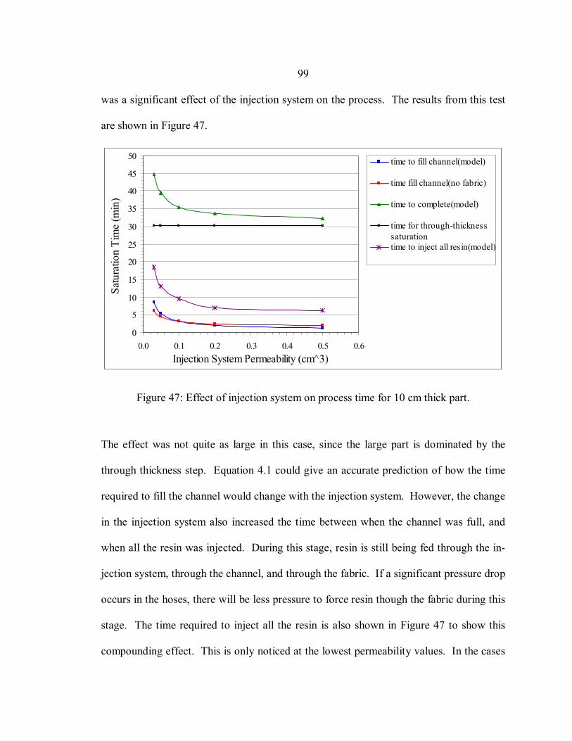
99
was a significant effect of the injection system on the process. The results from this test
are shown in Figure 47.
0
5
10
15
20
25
30
35
40
45
50
0.0 0.1 0.2 0.3 0.4 0.5 0.6Injection System Permeability (cm^3)
Satu
ratio
n Ti
me
(min
)
time to fill channel(model)
time fill channel(no fabric)
time to complete(model)
time for through-thicknesssaturationtime to inject all resin(model)
Figure 47: Effect of injection system on process time for 10 cm thick part.
The effect was not quite as large in this case, since the large part is dominated by the
through thickness step. Equation 4.1 could give an accurate prediction of how the time
required to fill the channel would change with the injection system. However, the change
in the injection system also increased the time between when the channel was full, and
when all the resin was injected. During this stage, resin is still being fed through the in-
jection system, through the channel, and through the fabric. If a significant pressure drop
occurs in the hoses, there will be less pressure to force resin though the fabric during this
stage. The time required to inject all the resin is also shown in Figure 47 to show this
compounding effect. This is only noticed at the lowest permeability values. In the cases
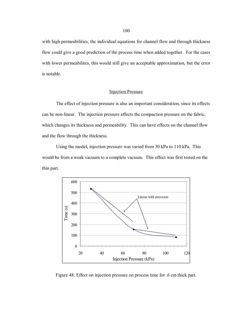
100
with high permeabilities, the individual equations for channel flow and through thickness
flow could give a good prediction of the process time when added together. For the cases
with lower permeabilites, this would still give an acceptable approximation, but the error
is notable.
Injection Pressure
The effect of injection pressure is also an important consideration, since its effects
can be non-linear. The injection pressure affects the compaction pressure on the fabric,
which changes its thickness and permeability. This can have effects on the channel flow
and the flow through the thickness.
Using the model, injection pressure was varied from 30 kPa to 110 kPa. This
would be from a weak vacuum to a complete vacuum. This effect was first tested on the
thin part.
0
100
200
300
400
500
600
20 40 60 80 100 120Injection Pressure (kPa)
Tim
e (s
)
Linear with pressure
Figure 48: Effect on injection pressure on process time for .6 cm thick part.
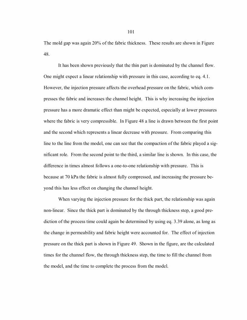
101
The mold gap was again 20% of the fabric thickness. These results are shown in Figure
48.
It has been shown previously that the thin part is dominated by the channel flow.
One might expect a linear relationship with pressure in this case, according to eq. 4.1.
However, the injection pressure affects the overhead pressure on the fabric, which com-
presses the fabric and increases the channel height. This is why increasing the injection
pressure has a more dramatic effect than might be expected, especially at lower pressures
where the fabric is very compressible. In Figure 48 a line is drawn between the first point
and the second which represents a linear decrease with pressure. From comparing this
line to the line from the model, one can see that the compaction of the fabric played a sig-
nificant role. From the second point to the third, a similar line is shown. In this case, the
difference in times almost follows a one-to-one relationship with pressure. This is
because at 70 kPa the fabric is almost fully compressed, and increasing the pressure be-
yond this has less effect on changing the channel height.
When varying the injection pressure for the thick part, the relationship was again
non-linear. Since the thick part is dominated by the through thickness step, a good pre-
diction of the process time could again be determined by using eq. 3.39 alone, as long as
the change in permeability and fabric height were accounted for. The effect of injection
pressure on the thick part is shown in Figure 49. Shown in the figure, are the calculated
times for the channel flow, the through thickness step, the time to fill the channel from
the model, and the time to complete the process from the model.
102
0.0
10.0
20.0
30.0
40.0
50.0
60.0
70.0
20 40 60 80 100 120
Injection Pressure (kPa)
Tim
e (s
)Time to fill channel (model)
time to fill channel (no fabric)
time to completion (model)
time for through-thicknesssaturation
Figure 49: Effect of injection pressure on process time for 10cm thick part.
Fabric Permeability
Another parametric study was done to determine the effect of the fabric perme-
ability on the process time. Again, the first case examined was for the .6 cm thick part
with 20% mold gap. The injection pressure was 70 kPa. The permeability was varied
from 1E-8 to 2E-7 cm2, which is the approximate range of permeabilities from the fabrics
tested. The results from this test are shown in Figure 50.
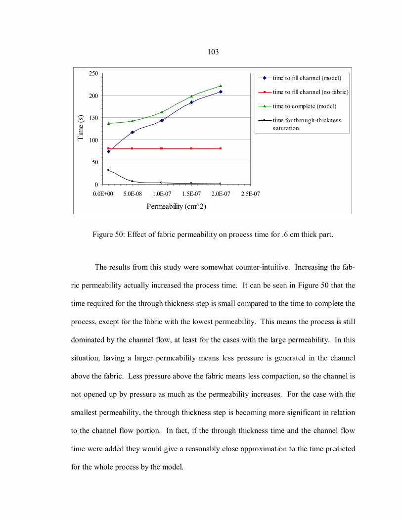
103
0
50
100
150
200
250
0.0E+00 5.0E-08 1.0E-07 1.5E-07 2.0E-07 2.5E-07
Permeability (cm^2)
Tim
e (s
)time to fill channel (model)
time to fill channel (no fabric)
time to complete (model)
time for through-thicknesssaturation
Figure 50: Effect of fabric permeability on process time for .6 cm thick part.
The results from this study were somewhat counter-intuitive. Increasing the fab-
ric permeability actually increased the process time. It can be seen in Figure 50 that the
time required for the through thickness step is small compared to the time to complete the
process, except for the fabric with the lowest permeability. This means the process is still
dominated by the channel flow, at least for the cases with the large permeability. In this
situation, having a larger permeability means less pressure is generated in the channel
above the fabric. Less pressure above the fabric means less compaction, so the channel is
not opened up by pressure as much as the permeability increases. For the case with the
smallest permeability, the through thickness step is becoming more significant in relation
to the channel flow portion. In fact, if the through thickness time and the channel flow
time were added they would give a reasonably close approximation to the time predicted
for the whole process by the model.
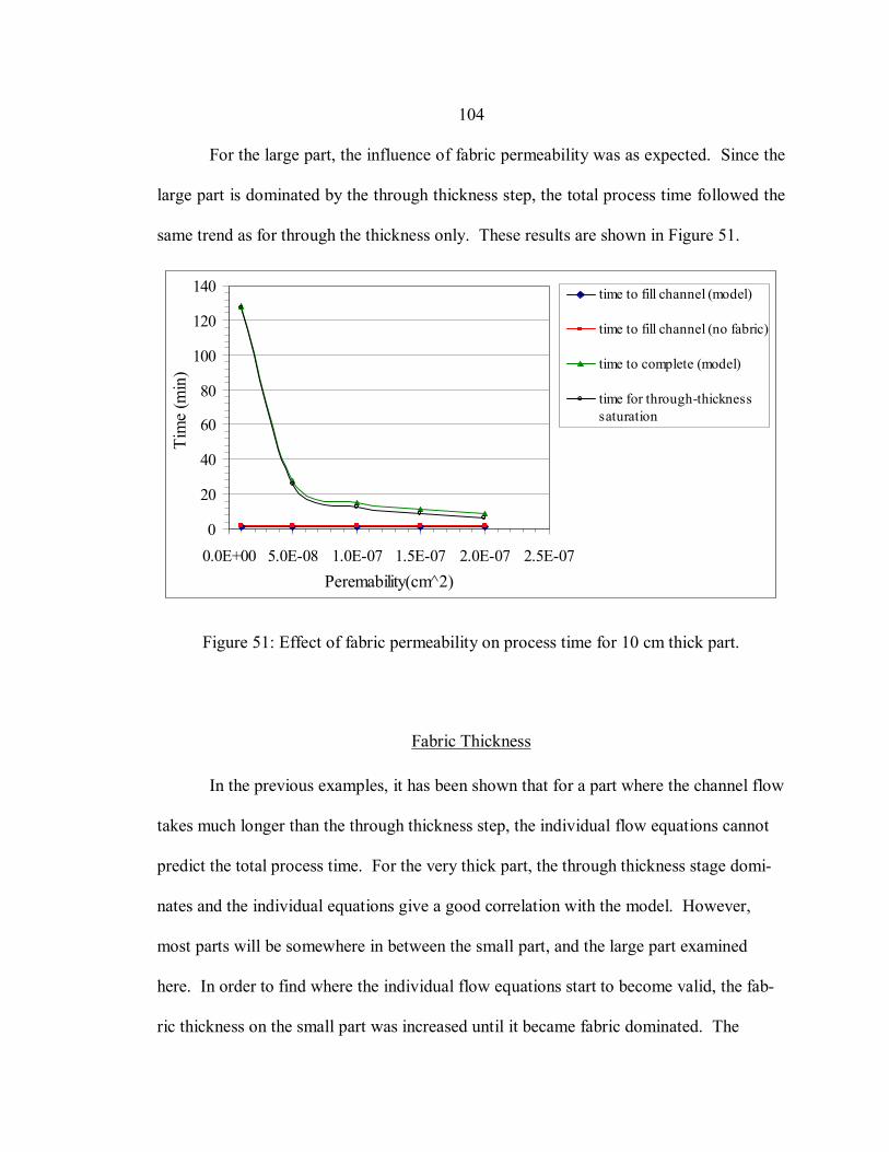
104
For the large part, the influence of fabric permeability was as expected. Since the
large part is dominated by the through thickness step, the total process time followed the
same trend as for through the thickness only. These results are shown in Figure 51.
0
20
40
60
80
100
120
140
0.0E+00 5.0E-08 1.0E-07 1.5E-07 2.0E-07 2.5E-07Peremability(cm^2)
Tim
e (m
in)
time to fill channel (model)
time to fill channel (no fabric)
time to complete (model)
time for through-thicknesssaturation
Figure 51: Effect of fabric permeability on process time for 10 cm thick part.
Fabric Thickness
In the previous examples, it has been shown that for a part where the channel flow
takes much longer than the through thickness step, the individual flow equations cannot
predict the total process time. For the very thick part, the through thickness stage domi-
nates and the individual equations give a good correlation with the model. However,
most parts will be somewhere in between the small part, and the large part examined
here. In order to find where the individual flow equations start to become valid, the fab-
ric thickness on the small part was increased until it became fabric dominated. The
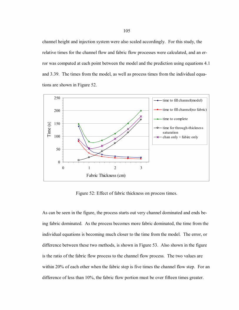
105
channel height and injection system were also scaled accordingly. For this study, the
relative times for the channel flow and fabric flow processes were calculated, and an er-
ror was computed at each point between the model and the prediction using equations 4.1
and 3.39. The times from the model, as well as process times from the individual equa-
tions are shown in Figure 52.
0
50
100
150
200
250
0 1 2 3
Fabric Thickness (cm)
Tim
e (s
)
time to fill channel(model)
time to fill channel(no fabric)
time to complete
time for through-thicknesssaturationchan only + fabirc only
Figure 52: Effect of fabric thickness on process times.
As can be seen in the figure, the process starts out very channel dominated and ends be-
ing fabric dominated. As the process becomes more fabric dominated, the time from the
individual equations is becoming much closer to the time from the model. The error, or
difference between these two methods, is shown in Figure 53. Also shown in the figure
is the ratio of the fabric flow process to the channel flow process. The two values are
within 20% of each other when the fabric step is five times the channel flow step. For an
difference of less than 10%, the fabric flow portion must be over fifteen times greater.
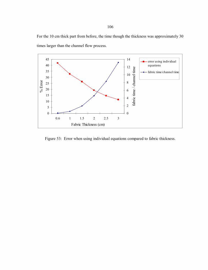
106
For the 10 cm thick part from before, the time though the thickness was approximately 30
times larger than the channel flow process.
0
5
10
15
20
25
30
35
40
45
0.6 1 1.5 2 2.5 3
Fabric Thickness (cm)
% E
rror
0
2
4
6
8
10
12
14
fabr
ic ti
me
/ cha
nnel
tim
e
error using individualequations
fabric time/channel time
Figure 53: Error when using individual equations compared to fabric thickness.
107
CHAPTER 7
DISCUSSION OF RESULTS
Fabric Tests
The fabric tests demonstrated multiple important aspects of flow through porous
media. Most important was the dramatic effect of compaction pressure on the fabric
permeability. For the fabrics tested, the permeability decreased by a factor of 2 to 3 be-
tween 30 kPa and 140 kPa. This effect could greatly influence decisions made by mold
designers. As the processing pressure increases a more robust mold will be required,
which will be more costly. If increasing the operating pressure does not significantly re-
duce the process time, the added cost of the mold may not be justified. However,
considerations such as the fiber volume fraction may dictate the compaction pressure
more than processing time.
The tests also showed that the fabric thickness and fiber volume fraction were
also greatly influenced by pressure. Fortunately, as the fabric is compressed the distance
that the resin must flow to saturate the part through the thickness decreases. Since the
saturation time was shown to be a function of the thickness squared, this can reduce the
effect of the decreased permeability. In order to illustrate how these effects interact, a
plot was generated to show the saturation time for a part with an initial thickness of 10
cm. For this example, the woven carbon was chosen since it had a large change in per-
meability and thickness with pressure. The trend from Figure 33 was extrapolated to
obtain guess values for the permeability at pressures greater than 350 kPa. The results
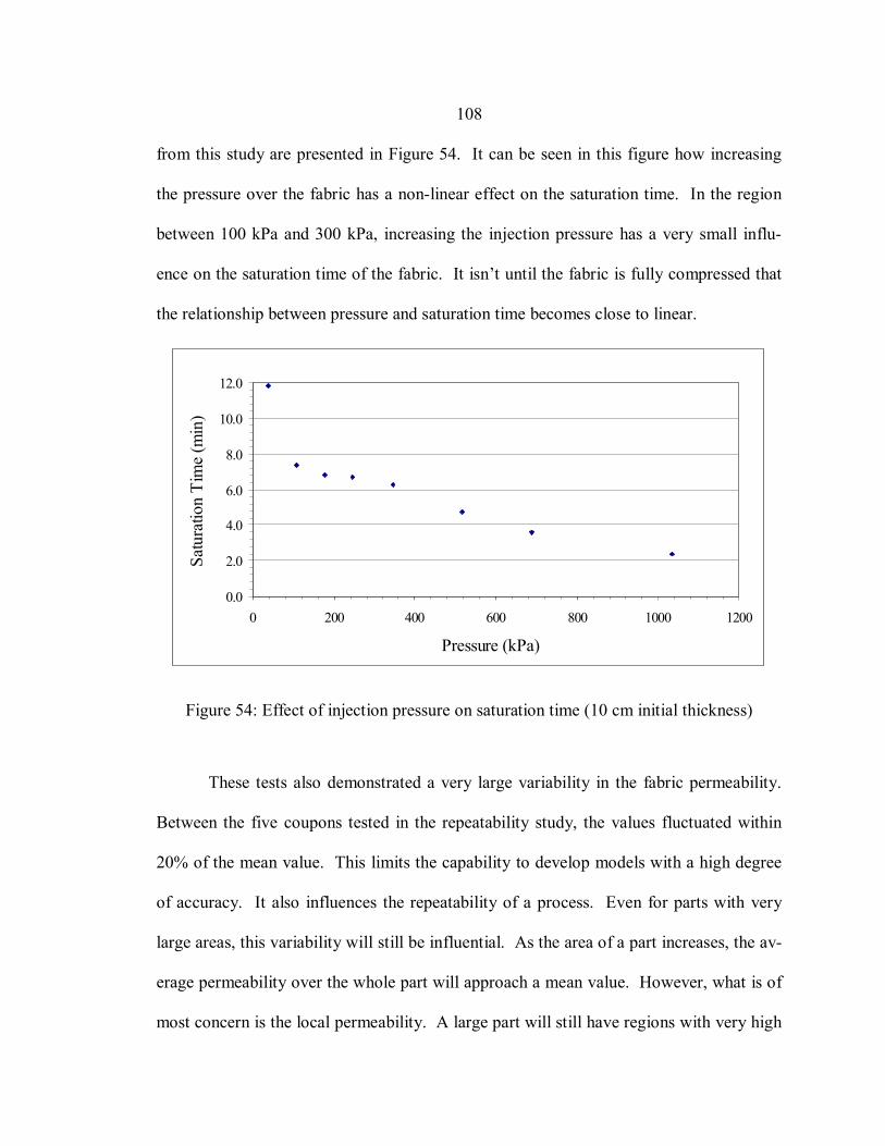
108
from this study are presented in Figure 54. It can be seen in this figure how increasing
the pressure over the fabric has a non-linear effect on the saturation time. In the region
between 100 kPa and 300 kPa, increasing the injection pressure has a very small influ-
ence on the saturation time of the fabric. It isn’t until the fabric is fully compressed that
the relationship between pressure and saturation time becomes close to linear.
0.0
2.0
4.0
6.0
8.0
10.0
12.0
0 200 400 600 800 1000 1200
Pressure (kPa)
Satu
ratio
n Ti
me
(min
)
Figure 54: Effect of injection pressure on saturation time (10 cm initial thickness)
These tests also demonstrated a very large variability in the fabric permeability.
Between the five coupons tested in the repeatability study, the values fluctuated within
20% of the mean value. This limits the capability to develop models with a high degree
of accuracy. It also influences the repeatability of a process. Even for parts with very
large areas, this variability will still be influential. As the area of a part increases, the av-
erage permeability over the whole part will approach a mean value. However, what is of
most concern is the local permeability. A large part will still have regions with very high
109
and low permeabilities. The larger the part, the greater the chances of having very ex-
treme local cases. If high permeability regions exist near low permeability regions, there
is a risk of entrapping air pockets. This was also found to be true for in-plane flow
through preforms composed of different fabrics [44]. This also means that the total proc-
ess time is going to be dictated by the region with the lowest permeability. An example
of this will be discussed shortly. With enough data, a statistical approach to processing
could be employed where a successful part would be produced 99% of the time, rather
than always planning on the worst possible case. Fortunately, since most of the variabil-
ity in the through thickness permeability is due to the random alignment of the flow
channels, as the part gets thicker this variability will decrease.
Air Permeability Testing
In both cases tested the permeability value from the air tests was about twice as
high as the interpolated value from the liquid tests. There are a couple explanations for
this result. The first is that Darcy’s law was intended for creeping flow, while the air in
these tests was moving at a very high velocity. In tests performed by Calhoun and
Yuster, the permeability values obtained with air were higher than the ones from liquid
tests. They attributed this to the fact that the mean free path of the air molecules was on
the same order of the spacing between fibers [18,47]. Another major contributor to the
larger values is flow around the edges. The edges were not siliconed as in the liquid tests
to keep with the idea of having a rapid test procedure, so the seal was not perfect. The
disks that were punched out and placed between the plies had a close fit with the inside
edge of the tube, but did not create a perfect seal. These disks could have also created
110
enough of a space between the plies to increase the permeability, since there was no pres-
sure to press the plies together. This would probably be a minor effect though since the
disks were only 0.07 mm thick. It is possible that siliconing the edges would have given
results much closer to those of the liquid tests, but this would have defeated the purpose
of the air tester which was to make testing much more rapid. The use of silicone would
have meant at least a day would have been required between tests. One other possibility
that was not examined would be to use a thick grease or something that could be smeared
around the edges to create a seal. This could not be used for the fluid tests because the
pressurized fluid would have pushed it out of the way and formed a channel. However,
for the air tests, since the pressures were very low a thick grease might have stayed in
place. This would add a little more time in preparation and cleanup, but would still result
in a very quick test.
The other drawback of the air tests is that they don’t give any indication of the
trend as the compaction pressure is increased. Since each fabric has a different trend at
higher pressures, there is no way to predict this from just the uncompressed value. The
test apparatus could be designed so that a mechanical clamping pressure could be applied
to the sample rather than relying on the fluid pressure. If the sample could be clamped
together by hydraulic cylinders it may be possible to know the clamping pressure, as well
as the sample thickness during a test. This clamping pressure could then be adjusted to
develop a curve. This is similar to the apparatus described by Hoes et al., although theirs
was for in-plane permeabilities [9,46]. Another possibility would be to clamp the sample
mechanically to a given thickness, and then determine the corresponding compaction
111
pressure through a separate test. This would be opposite to the approach used for the liq-
uid tests.
Although the air permeability tests did not duplicate the results from the liquid
tests, there is still potential in developing this technique. By improving the seals and al-
lowing the fabric to be mechanically compressed, the tests could still be performed with
relative ease compared to liquid tests. Ding et al. have achieved permeability results us-
ing air that were very close to the values from liquid tests [48]. One difference that made
their tests more successful is performing in-plane tests rather than through-thickness tests.
For in-plane tests they were able to flow air though the fabric over a long distance. This
allowed them to develop a pressure drop that was measurable, while still keeping a low
enough velocity for Darcy’s law to be valid. For the through thickness tests performed in
this study, the thickness of the samples was around 1 cm. This meant the velocity
through the fabric had to be very high in order to generate a measurable pressure drop.
The use of a much more sensitive pressure transducer, along with much thicker samples,
could improve the through thickness air tests.
Comprehensive Model
Overall, the comprehensive model did a very good job of predicting the flow
through the mold( e.g. Figure 37, Figure 38, Figure 40). The model was accurate in pre-
dicting the flow fronts for relatively thin parts, as well as thick parts. In all four tests, the
model predicted key events with errors typically less than 15%. Given the large variabil-
ity in the fabric, as well as the accumulation of errors in the input to the model, this was a
very good result. The model required experimental values as input for the equivalent
112
permeability of the injection system, the permeability of the fabric, the compressibility of
the fabric, the resin viscosity and the capillary pressure. Any errors in these values are
transferred to the model before it is even run. For this reason, it is hard to identify
whether the errors in the experiment are due to inaccurate input values or inadequacies
within the model. However, to achieve these results, both had to be reasonably accurate.
The first two tests involved relatively thin parts, with thin channels. Both of these
were represented well by the model. The fact that the part with less fabric and a thinner
channel had a greater error could be expected. As the channel gets thinner the assump-
tion that the transverse flow can be neglected in formulating equation 3.20 becomes less
valid. However, since the saturation time was still within 11% of the experimental value
this still appears to be a reasonable assumption. In both the first two tests, the model did
a fairly accurate job of predicting the flow front on the bottom of the mold as well (Fig-
ure 37 + Figure 38).
The results from the third experiment were very encouraging. In this case the
model predicted a saturation time right in the approximate range from the experiment.
There are a couple of reasons for this. Having a much larger channel would have reduced
the amount of transverse flow during stage one of the process. Since the fabric was also
thicker, this made the process more dominated by the through thickness step. Since there
were five tests done on this fabric the permeability of the fabric was well represented.
Also, the fabric compaction data was very clean and fit well with a logarithmic curve.
Although the fluid came through the fabric somewhat randomly at the end, there was no
air trapped in the mold. The results from this test were also good since the bagging was
113
not used to force the resin through the thickness, which eliminated any additional compli-
cation.
The fourth test involved all aspects of the process. The test was run to completion
with the use of the bagging to complete stage two of the process. When comparing the
model for the saturation time to the experiment, an error of 12 - 22% was seen. There are
several explanations for this. The first is the complication in the usage of the bagging.
Since the pressure had to be cut off and switched from the hoses to the bagging during
the process, there was a rather chaotic pressure profile to match. Another larger source of
error could have come from the fabric data used in this test. The fabric used in this test
was the woven roving which had less permeability data, and more scatter in the compac-
tion data. It was also noticed during the test that a small amount of edge leakage
occurred. This eventually caused the vents to be covered before the whole part was satu-
rated, leaving a strip of unsaturated fabric down the middle. This did not occur until the
very end of the process, so the amount of trapped air was small. Eventually, these re-
gions were wet out, possibly by capillary pressure. The small amounts of trapped air
must have resulted in micro-porosity, since no dry spots were found on subsequent in-
spection. The fact that small pockets of air were trapped would explain why it took much
longer to saturate these regions than the model predicted. It is also an important illustra-
tion of the effect of fabric variability and edge leakage. This occurred in large part due to
the fact that no vacuum was used to evacuate the air. The use of a vacuum would almost
eliminate this possibility, although an absolute vacuum cannot be used since it would boil
the resin.
114
Limitations of the Model
In applying this model to real manufacturing processes it will be important to un-
derstand the consequences of the assumptions, and where the limitations of the model
exist. This particular model has limitations due to the fact that it is only two dimensional;
however, these are not limitations of the modeling technique. The technique could be
extended to three dimensions, but his would come with a great increase in complexity.
One of the assumptions that was referred to earlier was the fact that the model
does not account for any racetracking. Since in the experiments the sides of the fabric
were siliconed, this was only a minor issue. However, in real processes using silicone
would not be practical. In the experiments, the part was relatively thick compared to its
width. For example, the thickness was around 2 cm while the width was only about 12.5
cm. For a part such as a wind turbine blade, or a boat hull, the width could be 100 times
the thickness. In this case, even if resin leaked around the edge it would have to flow
back towards the center of the part. Once the edges were saturated this flow would es-
sentially stop. Edge leakage could also be prevented in the design of the mold. If the
distribution channel did not extend all the way to the edge, the resin would be forced to
flow in the plane of the fabric before it could reach the edge. In addition, the mold could
also be made to clamp down on the edges to make them very impermeable. For these
reasons, the fact that the model does not account for racetracking is not considered to be a
major limitation.
Another consequence of the two dimensional model is that the flow in the channel
must be nearly one dimensional. In the experiments, the spacing of the injection hoses on
115
the leading edge of the mold was very much smaller than the length of the mold. This
made the flow front normal to the flow direction. This was also aided by the well at the
front of the mold. Although the resin entered the well at three points, it left as a uniform
flow front. This configuration was chosen for this model since it was geared to parts
such as turbine blades which are very long compared to their width. For parts of a differ-
ent geometry such as a square panel, the accuracy of the model would depend on the
injection system. If there were injection points at regular intervals along one edge of the
part, the model would still be quite accurate. If there was only one injection port the
model could loose much of its accuracy in stage one. In some processes the injection
ports may not be only at one end. They could be in the middle of the part, or in multiple
locations along the length of the part. This could be accounted for in the model simply
by changing the boundary conditions and adding more equations. Elements of hose could
be attached to any of the channel cells.
This particular model is also geared to processes where the distribution channel
covers the whole surface of the part, or close to it. This is most accurate for the pressure
bagging process and FASTRAC. In the parametric study, it was shown that for thick
parts this would be the fastest way to saturate a part. Thinner parts on the other hand,
may require a different strategy such as SCRIMP™. For processes such as SCRIMP™
where the distribution system is a series of channels which may have a large distance be-
tween them this model would not work. However, the same modeling technique could
still be used, but the two dimensions would be in the plane rather than one in the plane
and one in the thickness. This approach was used successfully by Han et al. to model the

116
processing of a boat hull using SCRIMP™ [7]. This method required all the same data
that was obtained here, but the permeability values were for in the plane.
It is almost impossible to come up with any general rules as to the limitations of
the model since everything is interrelated. What may be true for one case may not be true
for the other. This was illustrated in the parametric study. In any case, the designer
would have to use common sense and any past experience to assess how much error these
assumptions will cause.
For any case, a three dimensional model is going to provide the most accurate re-
sults. However, this comes at a cost. A three dimensional model will be much more time
consuming to create, and will take much more computational power to run. For example,
the model created here is not a true 2D model, since it does not account for flow in the
plane of the fabric. In order to make it a true 2D model the fabric would need to be bro-
ken into cells through the thickness. This would increase the number of equations by
increasing the number of cells. Also, each cell would have more unknowns since the
flow through all four faces would have to be determined. For a 3D model more cells
would have to be added in the width of the part, and each cell would have flows through
six faces. In addition to having more equations, if a finite difference technique were used
the matrix would no longer be banded. This means the process of solving for the un-
knowns in the matrix and storing the values would be less efficient as well. It will also
require much more testing to determine the permeability in all three principle directions.
The complexity of the model will most likely be beyond the capability of many manufac-
turing engineers, and may require independently developed software packages. In many
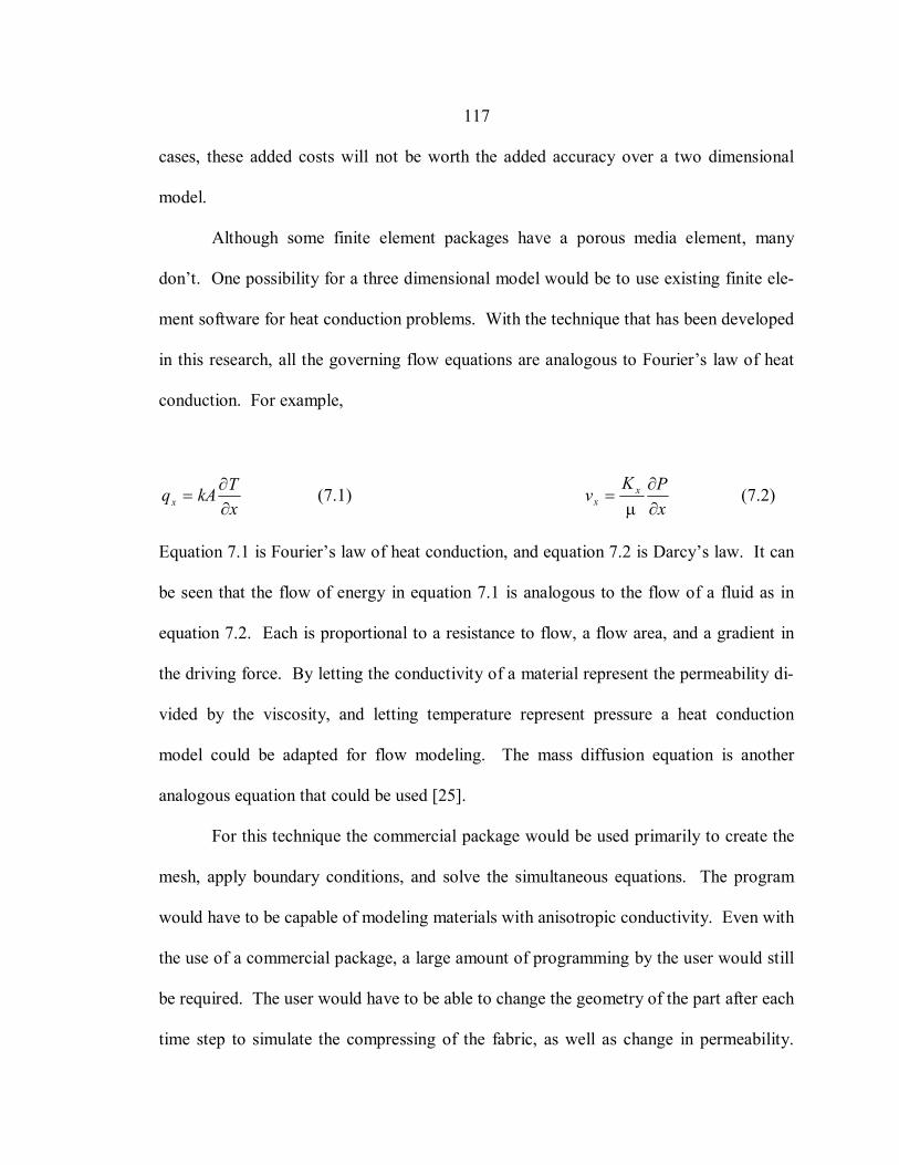
117
cases, these added costs will not be worth the added accuracy over a two dimensional
model.
Although some finite element packages have a porous media element, many
don’t. One possibility for a three dimensional model would be to use existing finite ele-
ment software for heat conduction problems. With the technique that has been developed
in this research, all the governing flow equations are analogous to Fourier’s law of heat
conduction. For example,
xTkAqx ∂∂
= (7.1) xPK x
x ∂∂
=µ
v (7.2)
Equation 7.1 is Fourier’s law of heat conduction, and equation 7.2 is Darcy’s law. It can
be seen that the flow of energy in equation 7.1 is analogous to the flow of a fluid as in
equation 7.2. Each is proportional to a resistance to flow, a flow area, and a gradient in
the driving force. By letting the conductivity of a material represent the permeability di-
vided by the viscosity, and letting temperature represent pressure a heat conduction
model could be adapted for flow modeling. The mass diffusion equation is another
analogous equation that could be used [25].
For this technique the commercial package would be used primarily to create the
mesh, apply boundary conditions, and solve the simultaneous equations. The program
would have to be capable of modeling materials with anisotropic conductivity. Even with
the use of a commercial package, a large amount of programming by the user would still
be required. The user would have to be able to change the geometry of the part after each
time step to simulate the compressing of the fabric, as well as change in permeability.
118
This approach has been used successfully by Liu [21]. However, that particular model
was for a closed mold process that did not have to deal with changing material properties.
One last limitation that was noticed with this model was that for very thin parts
with thin channels, the solution could become unstable. In these cases the matrices
would become ill conditioned. As a result, the solution vector could have negative or
imaginary solutions, which are physically impossible. The .6 cm thick part with the 10%
mold gap approached this condition. This condition was easy to spot since the solution
would not converge or would have an imaginary solution. To alleviate this effect, in-
creasing the number of cells in the channel helped, as well as adding a small amount of
initial saturation in the fabric. Fortunately, the cases where this occurred were ones
where this process would not be optimal anyway, as mentioned in the parametric study.
Parametric Study
In the parametric study a variety of parameters were examined. The purpose for
this study was twofold. The first was to observe how changing the individual parameters
affected the process as a whole. The other was to see how equations 3.39 and 4.1 might
be useful in predicting the effects of any changes to the process.
In every case the parameters that were varied had non-linear effects on the proc-
ess, some were predictable and some were not. The small part was found to be
dominated by channel flow. Therefore, anything that changed the channel geometry had
the largest effect. The fabric compaction under pressure significantly influenced the re-
sults since the equivalent permeability of the channel is quadratic with the channel height.
119
The large part was very dominated by the through thickness step. The influence of the
parameters was fairly predictable.
The individual flow equations were found to be useful in predicting trends, and in
some cases, gave accurate predictions for the whole process. For the thin part, the indi-
vidual equations gave predictions that were very far from the values given by the model.
This is because the thinner part was dominated by the channel flow. This means the time
required to flow through the thickness was very small compared to the time required to
fill the channel. As a result, the channel flow and fabric flow happened simultaneously.
This blurs the division between channel flow and fabric flow. The fabric essentially cre-
ates an additional volume that has to be filled by passing resin through the channel.
For the thick part, these equations had good agreement with the model. This is
due to the quadratic effect of fabric thickness on saturation time, which made the thick
part dominated by flow through the thickness. In this case, the time to fill the channel is
significantly less than the time to flow through the thickness. This also means only a
small portion of the fabric is saturated during the filling of the channel. As a result, the
process is almost divided into two distinct processes.
A study was done specifically to determine when the individual equations become
valid. It was found that if the through thickness step was fifteen times greater than the
channel flow step the individual equations were within 10% of the comprehensive model.
However, there may be exceptions to this rule. A summary of the results from the para-
metric study is shown in Table 5. In cases where the process is channel dominated, these
may only be useful in identifying trends, and not in giving definite increases in times.
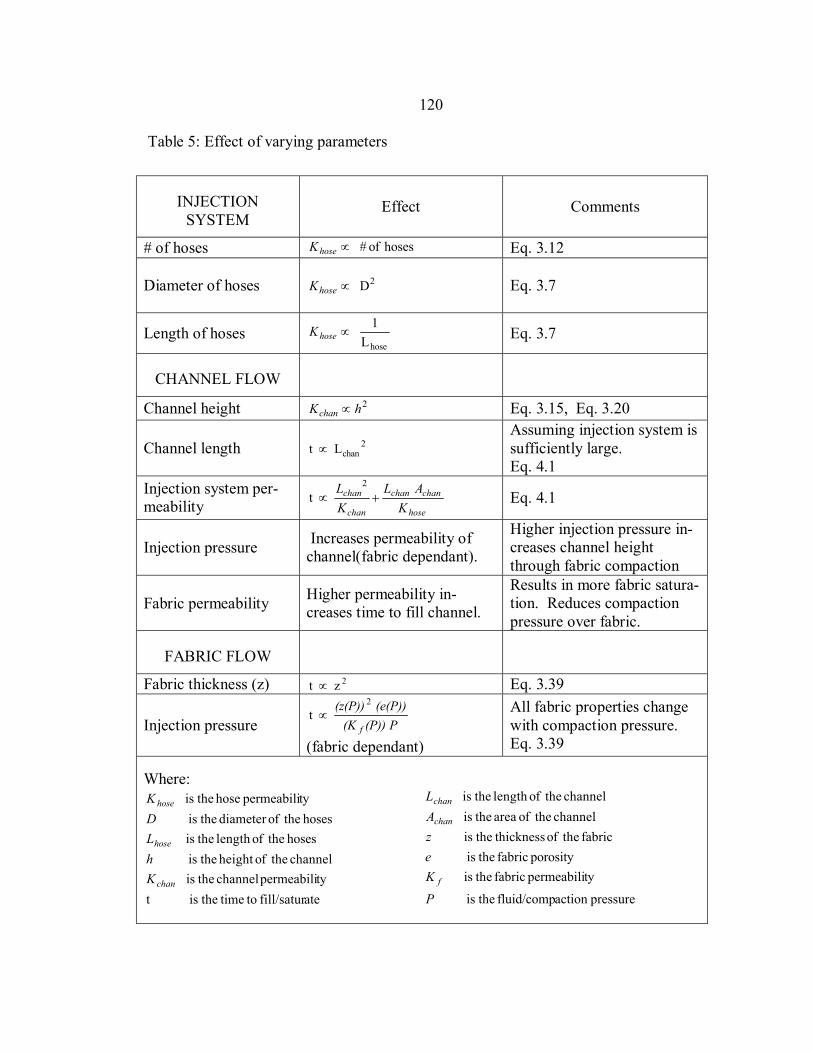
120
Table 5: Effect of varying parameters
INJECTION SYSTEM
Effect Comments
# of hoses hoses of # ∝hoseK Eq. 3.12
Diameter of hoses 2D ∝hoseK Eq. 3.7
Length of hoses hoseL1 ∝hoseK Eq. 3.7
CHANNEL FLOW
Channel height 2hKchan ∝ Eq. 3.15, Eq. 3.20
Channel length 2chanL t ∝
Assuming injection system is sufficiently large. Eq. 4.1
Injection system per-meability hose
chanchan
chan
chan
KAL
KL
+∝2
t Eq. 4.1
Injection pressure Increases permeability of channel(fabric dependant).
Higher injection pressure in-creases channel height through fabric compaction
Fabric permeability Higher permeability in-creases time to fill channel.
Results in more fabric satura-tion. Reduces compaction pressure over fabric.
FABRIC FLOW
Fabric thickness (z) z t 2∝ Eq. 3.39
Injection pressure t
2
P(P))(K(e(P))(z(P))
f∝
(fabric dependant)
All fabric properties change with compaction pressure. Eq. 3.39
Where:
atefill/satur to time theis t typermeabili channel theis
channel theofheight theis hoses theoflength theis
hoses theofdiameter theis typermeabili hose theis
chan
hose
hose
KhLDK
e
pressureaction fluid/comp theis
typermeabili fabric theis porosity fabric theis
fabric theof thickness theis channel theof area theis
channel theoflength theis
P
K
zAL
f
chan
chan
121
CHAPTER 8
CONCLUSIONS AND FUTURE WORK
Pressure bag molding, and similar processes, show great potential for meeting the
challenge of producing mega-watt scale wind turbine blades. In this study, the pressure
bag molding process has been examined and modeled in detail. The underlying physics
involved in the flow through the different regions of the process have been examined in-
dividually, and combined in a comprehensive model. The model created was successful
in duplicating a series of experiments, and in revealing the effects of certain critical pa-
rameters. Through the individual equations developed, and the computer model, scaling
effects in these types of processes can be determined. A procedure for locating and
minimizing rate limiting steps has also been developed.
Application to Manufacturing
To summarize the work performed in developing the numerical model, a process
outline has been created. The necessary data and tests that must be performed to con-
struct a similar model are presented here.
• Tests must be performed on the fabrics to determine the permeability in the direc-
tions where most of the flow is expected to occur. Permeability values must be
calculated at varying compaction pressures to create a curve fit.
• An approximate value for capillary pressure is needed. If the value is low com-
pared to the injection pressure, it may be insignificant. However, some fabric and
122
resin systems have high capillary pressures, so it is important to know at least an
approximate value to determine if it will be a factor.
• Tests relating compaction pressure to ply thickness and porosity must be con-
ducted. The data should be sufficient to create an accurate compaction curve,
especially at low pressures. If the compaction data can be obtained concurrently
with the permeability tests this would be optimal.
• From knowledge of the fabric properties and the largest distance that the resin
must flow though the fabric, the time for the fabric flow only can be determined.
• The equivalent permeability of the injection system must be determined either ex-
perimentally or by use of the equations developed here. Any fittings can create a
significant pressure drop and must be included in the analysis.
• The equivalent permeability of the distribution system must be determined. For
simple geometries Stokes flow equation can be used to calculate equivalent per-
meability. For more complex geometries, or high permeability layers, the
permeability may need to be calculated experimentally.
• By knowing the equivalent permeabilities of the injection system and channel(s),
and the length of the channel(s), the time for the channel flow process only can be
determined
• By comparing the individual times for the fabric flow and channel flow the proc-
ess the limiting step can be identified and minimized. For processes that are very
largely fabric flow dominated the individual equations can be reasonably accu-
123
rate. For parts that are channel flow dominated, the individual equations can pre-
dict trends but are inaccurate.
• For the most accurate predictions a 2D or 3D model must be used. The model
that is created must account for the effect of the net compaction pressure on per-
meability, fabric thickness, and porosity. These values should be continuously
updated throughout the process. It should be noted that dry fabric can be com-
pressed almost instantly, while saturated fabric takes time to compress. On the
other hand, dry fabric has a limited amount of spring-back when pressure is re-
duced, while saturated fabric may not spring back much at all. These effects must
be considered when creating a model.
Injection System / Channel Flow Modeling
The modeling of the injection system and the distribution channel used traditional
pipe flow theory based on Stokes flow. The subsequent experiments performed were
well represented by the analytical models. The fact that steady state equations were used
to model a transient process was not an issue. This was due to the low Reynolds numbers
involved and negligible surface tension effects. Also, the equations developed for flow
through the channel were still accurate despite the presence of the fabric. This was due to
the low permeability of the fabrics used.
Injection System / Channel Flow Future Work
For the cases examined, the equations for the injection system and channel were
sufficient. For cases with very thin channels, or very high permeability fabric, the chan-

124
nel equation may need to be modified. In these cases the flow into the fabric may be sig-
nificant enough to change the flow characteristics of the channel.
Fabric Tests
A major part of this work was to develop a permeability tester and use it to see
how compaction pressure would affect the flow through the fabric. Tests revealed a very
dramatic relationship between pressure and permeability. As the pressure was increased,
the permeability could decrease by almost an order of magnitude. This reduction was
most dramatic at lower pressures, and leveled of at high pressures when the fabric be-
came fully compressed. In the tests performed, the experimental data had a range of +/-
20% from the mean. This has important implications in using a single permeability value
to model a real process.
The capillary pressure proved to be very difficult to measure with the existing
setup. This was due to the short distance traveled, and the non-uniform flow front. This
test is further complicated by the dual scale flow involved in unsaturated tests.
The air permeability tests were not successful in duplicating the results from the
fluid tests. However, there is still potential in using air for permeability tests. Several
improvements were identified that would help the air tester to give accurate values, yet
still make testing very quick and easy. These are identified in the future work section.
It has also been found in this study that the compaction of fabric can have a dra-
matic effect on one-sided molding processes. Most fabrics will compress from 50% to
70% of their original thickness. This compaction influences the through thickness flow
step, as well as the channel flow stage by changing the channel geometry. The effect of
125
pressure is very extreme at low pressures, and eventually levels off once the fabric is
fully compressed. Fabric thickness versus pressure can be fitted with power law, or loga-
rithmic fits. However, it is best fit by non-linear techniques that divide the process into
three distinct regions.
Compaction pressure also has similar effects on the fabric porosity. As the pres-
sure is increased, the porosity is decreased. This increases the velocity through a preform
by reducing the effective flow area. Porosity also affects capillary pressure, but this may
be neglected in many cases since the capillary pressure is small to begin with.
Fabric Test Future Work
One of the largest sources for error in generating the data for the model was in
how the thickness was determined during the permeability tests. Rather than using com-
paction data from separate tests, it would be much better to measure the fabric thickness
directly during the test. This would require at least a modification to the existing appara-
tus, or possibly a new apparatus.
Fabric compaction tests should also be done on thick stacks of fabric (> 5 plies).
The data used in this study was generated from points taken from different fabric stacks.
This gives a good representation of the scatter in the data, and gives a good average
value. However, it may be better to develop a method where the same stack of fabric is
compressed through the range of pressures, so the data can be fit better with a curve. The
best fit would be a piecewise fit as presented by Chen et al. [15]. This method would also
require a minimum of tests.
126
The air permeability tester also deserves further development. Possible improve-
ments could come from thicker coupons, with lower velocities. This would require a
very sensitive pressure transducer, but may improve data by reducing the Reynolds num-
ber. Better sealing could also be accomplished by the use of a silicone grease around the
fabric. This should give a good seal, and still be fast to apply and clean up. The last im-
provement would be to compress the fabric mechanically. Either the fabric thickness or
the clamping pressure would need to be known in this case, or both.
Comprehensive Model
The experiments performed to validate the comprehensive model were in good
agreement with the model. The model did a good job of predicting the movement of the
flow fronts, and the time to saturate the part. Errors of less than 15% were typical. It
was observed that the variability of the fabric as well as edge effects can create non-
uniform flow fronts. A non-uniform flow front can cause the process to take measurably
longer than the model predicts. Although the permeability used in the model is an aver-
age value, the process could be limited by the region with the lowest permeability. It
tuned out to be very important to account for changes in permeability and fabric thickness
in the model. Both of these could change by a factor of two during the process. The as-
signment of the hoses and distribution channel with effective permeabilites proved to be a
valid technique. This enabled a control volume technique similar to the Hardy Cross
method to be used. Equivalent permeabilites could also be use with finite difference or
finite element analysis.
127
It was also shown that the individual governing equations for each region of the
mold could be useful in determining how changing parameters affects the process. For
processes that are largely channel flow dominated, these equations were only capable of
predicting trends. For parts that are largely dominated by the through thickness step,
these equations gave good predictions of the total process time.
Comprehensive Model Future Work
Improvements to the comprehensive model might be made by a more accurate
model of fabric compression. In the current model, the saturated fabric is considered to
be uncompressible, and assigned a uniform permeability. In reality, it may compress
slowly over time as it rejects extra resin. It may also have a varying permeability through
the thickness. To be very precise, these things would have to be accounted for. How-
ever, this would require a more sophisticated model, and may be overshadowed by much
larger sources of error such as fabric variability.
For modeling very thin parts, the matrices may need to be reconditioned or con-
strained to positive values. In extreme cases, the model could become unstable due to ill
conditioned matrices.
The model could also be adapted to account for the gelling of the resin. The resin
viscosity could easily be entered as a function of time rather than a constant value. This
would make the model more accurate for processes using real resin.
For testing purposes, a test mold with more pressure transducers above the chan-
nel would give more means of comparing the model to the experiment. In the tests
performed here, only the flow fronts and saturation time were compared.
128
REFERENCES CITED
1. B. D. Agarwal, L. J. Broutman, Analysis and Performance of Fiber Composites, Wiley, New York, 1980.
2. P.K Mallick, Fiber Reinforced Composites: Materials, Manufacturing, and De-sign, Marcel Dekker Inc., New York, 1988.
3. H.J. Sutherland, “On the Fatigue Analysis of Wind Turbines,” SAND99-0089, July 1999.
4. R.S. Parnas, Liquid Composite Molding, Carl Hanser, Munich, 2000.
5. D.A. Griffen, T.D. Ashwill, “Alternative Comoposite Materials for Megawatt-Scale Wind Turbine Blades: Design Considerations and Recommended Test-ing,” 2003 ASME Wind Energy Symposium, AIAA-2003-0696, 191-201.
6. D. S. Cairns, D.R. Humbert, J.F Mandell, “Modeling of Resin Transfer Molding of Composite Materials with Oriented Unidirectional Plies,” Composites Part A: Applied Science and Manufacturing, Mar 1999, Vol. 30, 375-383.
7. K. Han, S. Jiang, C. Zhang, B.Wang, “Flow Modeling and Simulation of SCRIMP™ for Composites Manufacturing,” Composites Part A, Jan 2000, Vol. 31, 79-86.
8. R. Pan, Z. Liang, C. Zhang, B. Wang, “Statistical Characterization of Fiber Permeability for Composite Manufacturing,” Polymer Composites, December 2000, Vol.21, No.6, 996-1006.
9. K. Hoes, D. Dineseu, H. Sol, M. Vanheule, R. Parnas, Y. Luo, I. Verpoest, “New Set-up for Measurement of Permeability Properties of Fibrous Rein-forcements for RTM,” Composites Part A 2002, Vol 33, No. 7, 959-969.
10. J.F. Mandell, D.D. Samborsky, D.S. Cairns, “Fatigue of Composite Materials and Substructures for Wind Turbine Blades,” SAND 2002-0771, March 2002
11. J. A. Schey, Introduction to Manufacturing Processes, McGraw-Hill, New York, 2000.
12. D.R. Askeland, The Science and Engineering of Materials, PWS Publishing Co., Boston, 1994
13. J.F. Mandell, D.D. Samborsky, N.K Wahl, H.J. Sutherland, "Testing and Analy-sis of Low Cost Composite Materials Under Spectrum Loading and High Cycle Fatigue Conditions," Proceedings of The 14th International Conference
129
on Composite Materials (ICCM-14), Society of Manufacturing Engineers, San Diego, California, July 14 - 18, 2003. Paper 1811. (2003)
14. J.D Skramstad, “Evaluation of Hand Lay-Up and Resin Transfer Molding in Composite Wind Turbine Blade Manufacturing,” Master’s Thesis in Me-chanical Engineering, Montana State University-Bozeman, August 1999.
15. B. Chen, A.H.-D. Cheng, T.-W. Chou, “A Nonlinear Compaction Model for Fi-brous Preforms,” Composites Part A: Applied Science and Manufacturing, May 2001, Vol. 32, 701-707.
16. B.R. Gebart, “Permeability of Unidirectional Reinforcements for RTM,” Jounal of Composite Materials, 1992,Vol. 26, No.8, 1100-1133.
17. E. Larson, “Pressure Bag Molding: Manufacturing, Mechanical Testing, Non-destructive Evaluation, and Analysis,” Master’s Thesis in Mechanical Engi-neering, Montana State University-Bozeman, January 2004.
18. S. Rossell, “Fluid Flow Modeling of Resin Transfer Molding for Composite Ma-terial Wind Turbine Blade Structures,” Master’s Thesis in Chemical Engineering, Montana State University-Bozeman, August 2000.
19. P. Simacek, E.M. Sozer, S.G. Advani, “User Manual for DRAPE 1.1 and LIMS 4.0 (Liquid Injection Molding Software),” University of Deleware Center for Composite Materials Technical Report, CCM Report 98-01, 1998.
20. S.G. Advani, Composite TechBrief: Liquid Injection Molding Simulation (LIMS), University of Deleware Center for Composite Materials, 2004, http://www.ccm.udel.edu/Pubs/techbriefs/LIMS.pdf
21. X.L. Liu, “Isothermal Flow Simulation of Liquid Composite Molding,” Com-posites Part A: Applied Science and Manufacturing, Dec 2000, Vol. 31, 1295-1302.
22. M. K. Kang, W.I Lee, H.T. Hahn, “Analysis of Vacuum Bag Resin Transfer Molding Process,” Composites Part A: Applied Science and Manufacturing, Nov 2001, Vol. 32, 1553-1560.
23. W.D Brouwer, E.C.F.C van Herpt, M. Labordus, “Vacuum Injection Moulding for Large Structural Applications,” Composites Part A: Applied Science and Manufacturing, Jun 2003, Vol. 34, 551-558.
24. H. Cross, “Analysis of Flow in Networks of Conduits or Conductors,” Univer-sity of Illinois Bulletin No. 286. November 1936.
130
25. R. B. Bird, W. E. Stewart, E. N. Lightfoot, Transport Phenomena, John Wiley & Sons, New York, 2002.
26. F. White, Fluid Mechanics, McGraw-Hill, New York, 1999.
27. H. D’arcy, Les Fontaines Publiques de la Ville de Dijon, Paris, 1856
28. A. Hammami, R. Gauvin, F. Trochu, “Modeling the Edge Effect in Liquid Composites Molding,” Composites Part A: Applied Science and Manufactur-ing, Jan 1998, Vol. 29, 603-609.
29. J.F. Delerue, S.V. Lomov, R.S. Parnas, I. Verpoest, and M. Wevers, “Pore Net-work Modeling of Permeability for Textile Reinforcements,” Polymer Composites, June 2003, Vol. 24, No. 3, 344-357.
30. P. Simacek, S. G. Advani, “Permeability Model for a Woven Fabric,” Polymer Composites, December 1996, Vol. 17, No. 6, 887-899.
31. P. Ferland, D. Guittard, F. Trochu, “Concurrent Methods for Permeability Measurement in Resin Transfer Molding,” Polymer Composites, February 1996, Vol. 17, No. 1, 149-158.
32. Y. Lai, B. Khomami, J. L. Kardos, “Accurate Permeability Characterization of Preforms Used in Polymer Matrix Composite Fabrication Processes,” Polymer Composites, June 1997, Vol. 18, No. 3, 368-377.
33. K. L. Adams, L. Rebenfeld, “Permeability Characteristics of Multilayer Fiber Reinforcements. Part 1: Experimental Observations,” Polymer Composites, June 1991, Vol. 12, No. 3, 179-185.
34. R. Parnas, K. Flynn, M. Dal-Favero, “A Permeability Database for Composites Manufacturing,” Polymer Composites, October 1997, Vol. 18, No.5, 623-633.
35. K. J. Ahn, J. C. Seferis, J. C. Berg, “Simultaneous Measurements of Permeabil-ity and Capillary Pressure of Thermosetting Matrices in Woven Fabric Reinforcements,” Polymer Composites, June 1991, Vol. 12, No. 3, 146-152.
36. L. Skartsis, B. Khomami, J.L. Kardos, “The Effect of Capillary Pressure on the Impregnation of Fibrous Media,” SAMPE Journal, October 1992, Vol. 28, No. 5, 19-23.
37. R.F. Probstein, Physiochemical Hydrodynamics, Butterworth-Heinemann, Bos-ton, 1989
131
38. R. Parnas, J.G. Howard, .T L. Luce, S. Advani, “Permeability Characterization. Part 1: A Proposed Standard Reference Fabric for Permeability,” Polymer Composites, December 1995, Vol. 16, No.6, 429-445.
39. Y. Luo, I. Verpoest, K. Hoes, M. Vanheule, H. Sol, A. Cardon, “ Permeability Measurement of Textile Reinforcements with Several Test Fluids,” Compos-ites Part A, 2001, Vol. 32, No. 10, 1497-1504.
40. J. A. Acheson, P. Simacek, S.G. Advani, “The Implications of Fiber Compac-tion and Saturation on Fully Coupled VARTM Simulation,” Composites Part A: Applied Science and Manufacturing, Feb 2004, Vol. 35, 159-169.
41. S. Bickerton, M.J. Buntain, A.A. Somashekar, “The Viscoelastic Compression Behavior of Liquid Composite Molding Preforms,” Composites Part A: Ap-plied Science and Manufacturing, May 2003, Vol. 34, 431-444.
42. C Lekakou, M. A. K. B. Johari, and M. G. Bader, “Compressibility and Flow Permeability of Two Dimensional Woven Reinforcements in the Processing of Composites,” Polymer Composites, October 1996, Vol. 17, No. 5, 666-672.
43. T. G. Gutowski, Z. Cai, J. Kingery, S. J. Wineman, “Resin Flow/Fiber Deforma-tion Experiments,” SAMPE Q 1986; 17(4), 54-58.
44. J. Mogavero, S. G. Advani, “Experimental Investigation of Flow through Multi-Layered Preforms,” Polymer Composites, October 1997, Vol. 18, No. 5, 649-655.
45. H. Lee, K. Neville, Handbook of Epoxy Resins, McGraw-Hill, New York, 1967
46. T. Luce, S. Advani, J. G. Howard, R. Parnas, “Permeability Characterization. Part 2: Flow Behavior in Multiple Layer Preforms,” Polymer Composites, De-cember 1995, Vol. 16, No. 6, 446-458.
47. J.C. Calhoun, S.T. Yuster, “A Study of the Flow of Homogeneous Fluids through Porous Media,” Drilling and Production Practice, 1946
48. L. Ding, C. Shih, Z. Liang, C. Zhang, B. Wang, “In Situ Measurement and Monitoring of Whole-Field Permeability Profile of Fiber Preform for Liquid Composite Molding,” Composites Part A: Applied Science and Manufactur-ing, Aug 2003, Vol. 34, 779-789.
49. J.R. Weitzenbock, R.A. Shenoi, P.A. Wilson, “Measurement of Three-Dimensional Permeability,” Composites Part A: Applied Science and Manu-facturing, Jan 1998, Vol. 29, 159-169.

132
APPENDICES

133
APPENDIX A
MATLAB PROGRAM FOR ENTIRE PROCESS
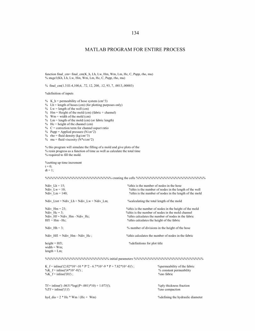
134
MATLAB PROGRAM FOR ENTIRE PROCESS
function final_cm= final_cm(K_h, Lh, Lw, Hm, Wm, Lm, Hc, C, Papp, rho, mu) % stage1(Kh, Lh, Lw, Hm, Wm, Lm, Hc, C, Papp, rho, mu) % final_cm(1.31E-4,100,6, .72, 12, 200, .12, 93, 7, .0013,.00003) %definition of inputs % K_h = permeability of hose system (cm^3) % Lh = length of hoses (cm) (for plotting purposes only) % Lw = length of the well (cm) % Hm = Height of the mold (cm) (fabric + channel) % Wm = width of the mold (cm) % Lm = length of the mold (cm) (or fabric length) % Hc = height of the channel (cm) % C = correction term for channel aspect ratio % Papp = Applied pressure (N/cn^2) % rho = fluid density (kg/cm^3) % mu = fluid viscosity (N*s/cm^2) % this program will simulate the filling of a mold and give plots of the % resin progress as a function of time as well as calculate the total time % required to fill the mold. %setting up time increment t = 0; dt = 1; %%%%%%%%%%%%%%%%%%%%%%%% creating the cells %%%%%%%%%%%%%%%%%%%%%%%%% Ndiv_Lh = 15; %this is the number of nodes in the hose Ndiv_Lw = 10; %this is the number of nodes in the length of the well Ndiv_Lm = 140; %this is the number of nodes in the length of the mold Ndiv_Ltot = Ndiv_Lh + Ndiv_Lw + Ndiv_Lm; %calculating the total length of the mold Ndiv_Hm = 23; %this is the number of nodes in the height of the mold Ndiv_Hc = 3; %this is the number of nodes in the mold channel Ndiv_Hf = Ndiv_Hm - Ndiv_Hc; %this calculates the number of nodes in the fabric Hf1 = Hm - Hc; %this calculates the height of the fabric Ndiv_Hh = 3; % number of divisions in the height of the hose Ndiv_Hf1 = Ndiv_Hm - Ndiv_Hc ; %this calculates the number of nodes in the fabric height = Hf1; %definitions for plot title width = Wm; length = Lm; %%%%%%%%%%%%%%%%%%%%%%% initial parameters %%%%%%%%%%%%%%%%%%%%%%%%% K_f = inline('(2.02*10^-10 * P^2 - 6.7*10^-9 * P + 7.82*10^-8)') ; %permeability of the fabric %K_f = inline('(4*10^-8)') ; % constant permeability %K_f = inline('(0)') ; %no fabric Tf = inline('(-.0631*log((P+.001)*10) + 1.073)'); %ply thickness fraction %Tf = inline('(1)') %no compaction hyd_dia = 2 * Hc * Wm / (Hc + Wm) %defining the hydraulic diameter

135
K_ch = (hyd_dia^2)*2/(C) %permeability of the channel del_x = Lm / Ndiv_Lm ; %length of each fabric column A_f = (Wm *del_x); %area of each fabric column A_ch = Wm * Hc ; %area of channel P_cap = .4; %capillary pressure fib_vol = .5; %fiber volume fraction e = 1 - fib_vol; %porosity fig = figure; set(gcf,'Color',[1,1,1]); cmap = [1 1 1; .75 .75 .75;0 .6 1;0 .3 1; 0 0 0 ]; %creating custom colors for plots colormap(cmap) V_inj = Hf1 * Wm * Lm * e *1.3 %volume of resin to inject %V_inj = .0022 %%%%%%%%%%%%%%%%%% Filling in Xposition matrix %%%%%%%%%%%%%%%%%%%%%%%%%% for j = 1 : Ndiv_Hm; for a = 1:Ndiv_Lh; Xpos(j,a) = (a)*Lh/(Ndiv_Lh); % nodes for hose end for b = Ndiv_Lh : Ndiv_Lh + Ndiv_Lw Xpos(j,b) = Lh + (b-Ndiv_Lh)*Lw/Ndiv_Lw; % nodes for well end for c = Ndiv_Lh + Ndiv_Lw : Ndiv_Ltot Xpos(j,c) = Lh + Lw + (c - Ndiv_Lh - Ndiv_Lw)*Lm/Ndiv_Lm; %nodes in mold end end %%%%%%%%%%%%%%%%%% creating Y position matrix %%%%%%%%%%%%%%%%%%%%%%%%%% for j = 1 : Ndiv_Ltot for a = 1 : Ndiv_Hc Ypos(a,j) = Hm - a*Hc/Ndiv_Hc; %nodes in the channel end for b = 1 : Ndiv_Hf1 Ypos(b + Ndiv_Hc,j) = Hm - Hc - b*Hf1/Ndiv_Hf; %nodes in the fabric end end %%%%%%%%%%%%%%%% Creating the fill matrix for plotting %%%%%%%%%%%%%%%%%%%%%%%%% % creating fill matrix color background for i = 1:Ndiv_Hm+9 for j = 1:Ndiv_Ltot+7 F(i, j) = 1; end end % creating fill matrix color for hose for i = 1 : Ndiv_Lh for j = Ndiv_Hm-Ndiv_Hh : Ndiv_Hm F(j+4,i)=0; end end % creating fill matrix color for well for i = Ndiv_Lh + 1 : Ndiv_Lh + Ndiv_Lw for j = 1 : Ndiv_Hm F(j+4,i) = 0; end end % creating fill matrix color for mold gap for i = Ndiv_Lh + Ndiv_Lw + 1 : Ndiv_Ltot for j = 1 : Ndiv_Hc F(j+4,i) = 0; end

136
end F(1,Ndiv_Ltot) = 0; %creating vent F(2,Ndiv_Ltot) = 0; F(3,Ndiv_Ltot) = 0; F(4,Ndiv_Ltot) = 0; % creating fill matrix color for fabric for i = 1 : Ndiv_Lm for j = Ndiv_Hc+1 : Ndiv_Hm F(j+4,i + Ndiv_Lh + Ndiv_Lw) = .25; end end %%%%%%%%%%%%%%%%%%%%%%%% filling the hoses %%%%%%%%%%%%%%%%%%%%%%%%% %updating fill matrix for hose for i = 1 : Ndiv_Lh for j = Ndiv_Hm-Ndiv_Hh : Ndiv_Hm F(j+4,i)=.75; end end %%%%%%%%%%%%%%%%%%%%%%%% filling up the well %%%%%%%%%%%%%%%%%%%%%%%%% Vol_well = Hm * Wm * Lw; %defining volume of well flow_hose = K_h * Papp / mu; %defining flow rate through hoses height_well = 0; %setting initial height of the well while height_well < Hm t = t+dt; flow_hose = K_h * Papp / mu; height_well = flow_hose * t / (Wm*Lw); % height of fluid in well %updating fill matrix for i = Ndiv_Lh + 1 : Ndiv_Lh + Ndiv_Lw for j = 1 : Ndiv_Hm if height_well > Ypos(j,i) F(j+4,i) = .75; end end end end %%%%%%%%%%%%%%%%%%%%%%%%%%%%%%%%%%%%%%%%%%%%%%%%%%%%%%%%%% %%%%%%%%%%%%%%%%%%filling the mold gap and fabric (Stage 1A) %%%%%%%%%%%%%%%%%%% %%%%%%%%%%%%%%%%%%%%%%%%%%%%%%%%%%%%%%%%%%%%%%%%%%%%%%%%%% ti = t; % defining initial time mu2 = mu*1; % correction for different temperature in mold V_tot = 0; % defining initial value for total volume dt = 1; % re-defining time step x_chan = .02*Lm; % initial value of x_chan to avoud division by zero in first calculation P(Ndiv_Hm,Ndiv_Lm) = zeros; %initial values in the pressure matrix above fabric P_chan = .01*Papp; %initial pressure in the mold for i = 1:Ndiv_Lm K_f_P(1,i) = K_f(P_chan); %initial permeability matrix Tf_P_new(1,i) = 1; % initial thickness fraction matrix Ycol(1,i) = .04 * ( Hf1 ); % initial penetration into the fabric to avoid division by zero
137
Hf_u_new(1,i) = Hf1*.96; %initial height of unsaturated fabric H_chan(1,i) = Hc ; %initial channel height above each column hyd_dia_mat(1,i) = 2 * Hc * Wm / (Hc+ Wm); %defining the hydraulic diameter K_ch_mat(1,i) = (hyd_dia^2)*2/(C) ; %permeability of the channel A_ch_mat(1,i) = Wm * Hc; % area of channel above column end %%%%%%%%%%%%%%%%%%%%%%%%%% entering first loop %%%%%%%%%%%%%%%%%%%%%% while x_chan < Lm if V_tot > V_inj %checking to see if all the resin has been injected break end x_cells = x_chan/del_x; %calculating the number of cells needed in the matrix x_cells = round(x_cells); %rounding to nearest integer for i = 1:3*x_cells+2 %setting initial matrix values to zero for j = 1:3*x_cells+2 Coef_mat( i, j) = 0; S_mat(i,1) = 0; end end %generating solution vector S_mat(3*x_cells+1,1) = Papp*K_h/mu; for i = 1 : x_cells if Hf_u_new(1,i) > 0 %checking to see if resin has reached the bottom of the mold S_mat(i,1) = A_f * K_f_P(1,i) * P_cap / (mu * Ycol(1,i)); else S_mat(i,1) = 0; %if resin has reached bottom Kf for that cell is zero end end %%%%%%%%%%%%%%%%%%%%% generating coefficient matrix %%%%%%%%%%%%%%%%%%%%%% for d = 1 : x_cells Coef_mat(d,d) = 1; if Hf_u_new(1,d) > 0 %checking to see if resin has reached the bottom of the mold Coef_mat(d,2*x_cells + 1+d) = -A_f * K_f_P(1,d) / ( 2 * mu2 * Ycol(1,d)); Coef_mat(d,2*x_cells + 2+d) = -A_f * K_f_P(1,d) / ( 2 * mu2 * Ycol(1,d)); else Coef_mat(d,2*x_cells + 1+d) = 0; %if resin has reached bottom Kf for that cell is zero Coef_mat(d,2*x_cells + 2+d) = 0; end Coef_mat(x_cells+d,d) = -1; Coef_mat(x_cells+d,x_cells+d) = 1 ; Coef_mat(x_cells+d,x_cells+1+d) = -1; Coef_mat(2*x_cells+d,x_cells+1+d) = 1; Coef_mat(2*x_cells+d,2*x_cells+1+d) = -A_ch_mat(1,d)*K_ch_mat(1,d)/(mu*del_x); Coef_mat(2*x_cells+d,2*x_cells+2+d) = A_ch_mat(1,d)*K_ch_mat(1,d)/(mu*del_x); Coef_mat(3*x_cells+1 , x_cells+1) = 1; Coef_mat(3*x_cells+1 , 2*x_cells+2) = K_h/mu; Coef_mat(3*x_cells+2 , 3*x_cells+2) = 1;
138
end Coef_mat; S_mat; Unk_mat = Coef_mat\S_mat; %now calculate the flow into each column of fabric flow_fabric = 0; %initial value for i = 1:x_cells v_column(1,i) = Unk_mat(i,1)/(A_f*e); %porosity term added to get actual velocity for each column Ycol(1,i) = Ycol(1,i) + v_column(1,i)*dt; del_Ycol(1,i) = v_column(1,i)*dt; end %%%%%%%%%%%%%%%%%% accounting for fabric compressing %%%%%%%%%%%%%%%%%%%%% for i = 1:x_cells %updating permeability of each column as function of pressure K_f_P(1,i) = K_f(Unk_mat(2*x_cells+1+i)); end Tf_P_old = Tf_P_new; Hf_u_old = Hf_u_new; vol_add = 0; for i = 1: x_cells % thickness fraction matrix Tf_P_new(1,i) = Tf(Unk_mat(2*x_cells+1+i)); if Tf_P_new(1,i)>1 % thickness fraction cannot exceed one Tf_P_new(1,i) = 1; else Tf_P_new(1,i) = Tf_P_new(1,i); end Hf_u_new (1,i)= (Hf_u_old(1,i) - del_Ycol(1,i)) * Tf_P_new(1,i) / Tf_P_old(1,i) ; H_chan(1,i) = Hm -Ycol(1,i) - Hf_u_new(1,i); %height of channel above fabric hyd_dia_mat(1,i) = 2 * H_chan(1,i) * Wm / (H_chan(1,i) + Wm); %defining the hydraulic diameter K_ch_mat(1,i) = (hyd_dia_mat(1,i)^2)*2/(C) ; %permeability of the channel A_ch_mat(1,i) = Wm * H_chan(1,i); % area of channel above column delta_Hf = (Hf_u_old(1,i) - del_Ycol(1,i)) - Hf_u_new(1,i); % calculating the change in fabric height vol_add = vol_add + delta_Hf * Wm*del_x; %calculating the extra volume created end t = t + vol_add / flow_hose ; % accounting for time to fill new volume V_tot = V_tot + vol_add; %%%%%%%%%%%%%%%%%%%%%% flow through channel %%%%%%%%%%%%%%%%%%%%%%%%% flow_chan = Unk_mat(2*x_cells+1,1); %calculating the flow through the last cell of channel flow_h = Unk_mat(x_cells+1,1); V_tot = V_tot + flow_h * dt; P_1 = Unk_mat(2*x_cells+2,1); x_chan = x_chan + flow_chan / A_ch_mat(1,x_cells)* dt; %calculating new position of fluid front %%%%%%%%%%%%%%%%%%%%%%%%%%%%%%%%%%%%%%%%%%%%%%%%%%%%%%%%% %%%%%%%%%%%%%%%%%%%%%%%% graphic dispay %%%%%%%%%%%%%%%%%%%%%%%%%% % updating fill matrix through mold gap for i = Ndiv_Lh + Ndiv_Lw + 1 : Ndiv_Ltot for j = 1 : Ndiv_Hc

139
if Xpos(j,i) < Lh + Lw + x_chan F(j+4,i) = .75; else F(j+4,i) = 0; end end end % Updating fill matrix into fabric for i = 1 : Ndiv_Lm for j = Ndiv_Hc+1 : Ndiv_Hm if Hm - Hc - Ycol(1,i) < Ypos(j,i + Ndiv_Lh + Ndiv_Lw) F(j+4,i + Ndiv_Lh + Ndiv_Lw) = .5; else F(j+4,i + Ndiv_Lh + Ndiv_Lw) = .25; end end end t = t + dt end % end of time step tmin = round(t/60) t = round(t) subplot(3,1,1) pcolor(F) title(['Part Dimensions: ' ,num2str(height),'cm X ',num2str(width),'cm X ',num2str(length),'cm time =',num2str(t),'s']) h = findobj(gca,'Type','surface','EdgeAlpha',1); set(h,'EdgeAlpha',0.0) set(gca,'XColor',[1,1,1],'YColor',[1,1,1]) axis ij equal tight % plot of pressure vs. position % for i = 1:x_cells+1 %creating pressure vs. position graph % P_vs_x(i+1,1) = Unk_mat(2*x_cells+1+i,1)*10; % x(i+1,1) = Ndiv_Lh + Ndiv_Lw + (i-1); % end % P_vs_x(1,1) = Papp*10; % x(1,1) = 0; % x(2,1) = Ndiv_Lh; %subplot(3,1,2) %plot(x,P_vs_x); %axis([0,Ndiv_Lh+Ndiv_Lw+Ndiv_Lm,0,Papp*1.2*10]); %ylabel('Pressure (kPa)'); %xlabel('x cell number'); %title('Pressure vs. Position') %%%%%%%%%%%%%%%%%%%%%%%%%%%%%%%%%%%%%%%%%%%%%%%%%%%%%%%%%% %%%%%%%%%%%%%%%%%% filling the mold gap and fabric (Stage 1B ) %%%%%%%%%%%%%%%%%% %%%%%%%%%%%%%%%%%%%%%%%%%%%%%%%%%%%%%%%%%%%%%%%%%%%%%%%%%% x_chan = Lm; x_cells = Ndiv_Lm; % takes care of any rounding problems from previous loop ti2 = (t-ti)/dt; dt = 1 ; % re-defining time step while Hf_u_new(1,Ndiv_Lm) > 0 t = t + dt if V_tot > V_inj %checking to see if all the resin has been injected break end for i = 1:3*x_cells+2 %setting initial matrix values to zero for j = 1:3*x_cells+2 Coef_mat( i, j) = 0; S_mat(i,1) = 0;
140
end end %generating solution vector S_mat(3*x_cells+1,1) = Papp*K_h/mu; for i = 1 : x_cells if Hf_u_new(1,i) > 0 %checking to see if resin has reached the bottom of the mold S_mat(i,1) = A_f * K_f_P(1,i) * P_cap / (mu * Ycol(1,i)); else S_mat(i,1) = 0; %if resin has reached bottom Kf for that cell is zero end end %%%%%%%%%%%%%%%%%%%%% generating coefficient matrix %%%%%%%%%%%%%%%%%%%%%% for d = 1 : x_cells Coef_mat(d,d) = 1; if Hf_u_new(1,d) > 0 %checking to see if resin has reached the bottom of the mold Coef_mat(d,2*x_cells + 1+d) = -A_f * K_f_P(1,d) / ( 2 * mu2 * Ycol(1,d)); Coef_mat(d,2*x_cells + 2+d) = -A_f * K_f_P(1,d) / ( 2 * mu2 * Ycol(1,d)); else Coef_mat(d,2*x_cells + 1+d) = 0; %if resin has reached bottom Kf for that cell is zero Coef_mat(d,2*x_cells + 2+d) = 0; end Coef_mat(x_cells+d,d) = -1; Coef_mat(x_cells+d,x_cells+d) = 1 ; Coef_mat(x_cells+d,x_cells+1+d) = -1; Coef_mat(2*x_cells+d,x_cells+1+d) = 1; Coef_mat(2*x_cells+d,2*x_cells+1+d) = -A_ch_mat(1,d)*K_ch_mat(1,d)/(mu*del_x); Coef_mat(2*x_cells+d,2*x_cells+2+d) = A_ch_mat(1,d)*K_ch_mat(1,d)/(mu*del_x); Coef_mat(3*x_cells+1 , x_cells+1) = 1; Coef_mat(3*x_cells+1 , 2*x_cells+2) = K_h/mu; Coef_mat(3*x_cells+2 , 2*x_cells+1) = 1; end Unk_mat = Coef_mat\S_mat; %solving for unknowns %now calculate the flow into each column of fabric flow_fabric = 0; %initial value for i = 1:x_cells v_column(1,i) = Unk_mat(i,1)/(A_f*e); %porosity term added to get actual velocity Ycol(1,i) = Ycol(1,i) + v_column(1,i)*dt; del_Ycol(1,i) = v_column(1,i)*dt; end %%%%%%%%%%%%%%%%%% accounting for fabric compressing %%%%%%%%%%%%%%%%%%%%% for i = 1:x_cells %updating permeability of each column as function of pressure K_f_P(1,i) = K_f(Unk_mat(2*x_cells+1+i)); end Tf_P_old = Tf_P_new; Hf_u_old = Hf_u_new; vol_add = 0; for i = 1: x_cells % thickness fraction matrix Tf_P_new(1,i) = Tf(Unk_mat(2*x_cells+1+i));
141
if Tf_P_new(1,i)>1 % thickness fraction cannot exceed one Tf_P_new(1,i) = 1; else Tf_P_new(1,i) = Tf_P_new(1,i); end Hf_u_new (1,i)= (Hf_u_old(1,i) - del_Ycol(1,i)) * Tf_P_new(1,i) / Tf_P_old(1,i) ; H_chan(1,i) = Hm -Ycol(1,i) - Hf_u_new(1,i); %height of channel above fabric hyd_dia_mat(1,i) = 2 * H_chan(1,i) * Wm / (H_chan(1,i) + Wm); %defining the hydraulic diameter K_ch_mat(1,i) = (hyd_dia_mat(1,i)^2)*2/(C) ; %permeability of the channel A_ch_mat(1,i) = Wm * H_chan(1,i); % area of channel above column delta_Hf = (Hf_u_old(1,i) - del_Ycol(1,i)) - Hf_u_new(1,i); % calculating the change in fabric height vol_add = vol_add + delta_Hf * Wm*del_x; %calculating the extra volume created end flow_hose = K_h * Papp / mu; t = t + vol_add / flow_hose ; % accounting for time to fill new volume V_tot = V_tot + vol_add; %%%%%%%%%%%%%%%%%%%%% flow through channel %%%%%%%%%%%%%%%%%%%%%%%%%% flow_chan = Unk_mat(2*x_cells+1,1); flow_h = Unk_mat(x_cells+1,1); V_tot = V_tot + flow_h * dt; P_1 = Unk_mat(2*x_cells+2,1); x_chan = x_chan + flow_chan / A_ch_mat(1,x_cells)* dt; %calculating new position of fluid front v_column; %%%%%%%%%%%%%%%%%%%%%%%%%%%%%%%%%%%%%%%%%%%%%%%%%%%%%%%%%% %%%%%%%%%%%%%%%%%%%%%%%% graphic dispay %%%%%%%%%%%%%%%%%%%%%%%%%% % Updating fill matrix into fabric for i = 1 : Ndiv_Lm for j = Ndiv_Hc+1 : Ndiv_Hm if Hm - Hc - Ycol(1,i) < Ypos(j,i + Ndiv_Lh + Ndiv_Lw) F(j+4,i + Ndiv_Lh + Ndiv_Lw) = .5; else F(j+4,i + Ndiv_Lh + Ndiv_Lw) = .25; end end end end % end of time step tmin = round(t/60) t = round(t) subplot(3,1,2) pcolor(F) title(['Part Dimensions: ' ,num2str(height),'cm X ',num2str(width),'cm X ',num2str(length),'cm time =',num2str(t),'s']) h = findobj(gca,'Type','surface','EdgeAlpha',1); set(h,'EdgeAlpha',0.0) set(gca,'XColor',[1,1,1],'YColor',[1,1,1]) axis ij equal tight pause %%%%%%%%%%%%%%%%%%%%%%%%%%%%%%%%%%%%%%%%%%%%%%%%%%%%%%%%%% %%%%%%%%%%%%%%% Apply pressure to the bagging (Stage 2) %%%%%%%%%%%%%%%%%%%%%% %%%%%%%%%%%%%%%%%%%%%%%%%%%%%%%%%%%%%%%%%%%%%%%%%%%%%%%%%% while Hf_u_new(1,Ndiv_Lm) > 0 t = t + dt
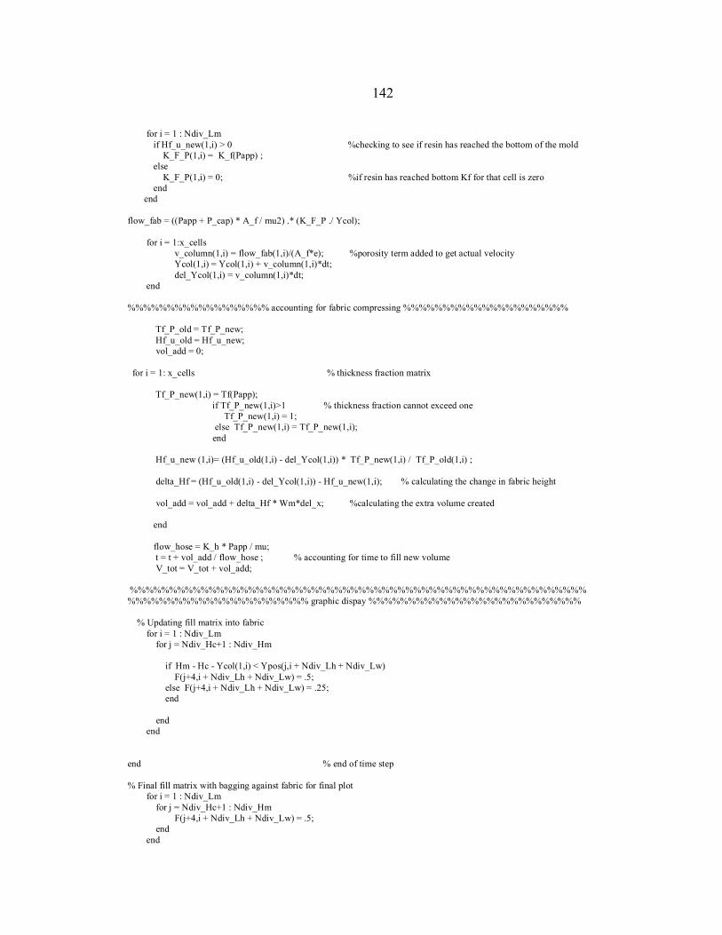
142
for i = 1 : Ndiv_Lm if Hf_u_new(1,i) > 0 %checking to see if resin has reached the bottom of the mold K_F_P(1,i) = K_f(Papp) ; else K_F_P(1,i) = 0; %if resin has reached bottom Kf for that cell is zero end end flow_fab = ((Papp + P_cap) * A_f / mu2) .* (K_F_P ./ Ycol); for i = 1:x_cells v_column(1,i) = flow_fab(1,i)/(A_f*e); %porosity term added to get actual velocity Ycol(1,i) = Ycol(1,i) + v_column(1,i)*dt; del_Ycol(1,i) = v_column(1,i)*dt; end %%%%%%%%%%%%%%%%%% accounting for fabric compressing %%%%%%%%%%%%%%%%%%%%% Tf_P_old = Tf_P_new; Hf_u_old = Hf_u_new; vol_add = 0; for i = 1: x_cells % thickness fraction matrix Tf_P_new(1,i) = Tf(Papp); if Tf_P_new(1,i)>1 % thickness fraction cannot exceed one Tf_P_new(1,i) = 1; else Tf_P_new(1,i) = Tf_P_new(1,i); end Hf_u_new (1,i)= (Hf_u_old(1,i) - del_Ycol(1,i)) * Tf_P_new(1,i) / Tf_P_old(1,i) ; delta_Hf = (Hf_u_old(1,i) - del_Ycol(1,i)) - Hf_u_new(1,i); % calculating the change in fabric height vol_add = vol_add + delta_Hf * Wm*del_x; %calculating the extra volume created end flow_hose = K_h * Papp / mu; t = t + vol_add / flow_hose ; % accounting for time to fill new volume V_tot = V_tot + vol_add; %%%%%%%%%%%%%%%%%%%%%%%%%%%%%%%%%%%%%%%%%%%%%%%%%%%%%%%%%% %%%%%%%%%%%%%%%%%%%%%%% graphic dispay %%%%%%%%%%%%%%%%%%%%%%%%%%% % Updating fill matrix into fabric for i = 1 : Ndiv_Lm for j = Ndiv_Hc+1 : Ndiv_Hm if Hm - Hc - Ycol(1,i) < Ypos(j,i + Ndiv_Lh + Ndiv_Lw) F(j+4,i + Ndiv_Lh + Ndiv_Lw) = .5; else F(j+4,i + Ndiv_Lh + Ndiv_Lw) = .25; end end end end % end of time step % Final fill matrix with bagging against fabric for final plot for i = 1 : Ndiv_Lm for j = Ndiv_Hc+1 : Ndiv_Hm F(j+4,i + Ndiv_Lh + Ndiv_Lw) = .5; end end

143
for i = Ndiv_Lh + 1 : Ndiv_Ltot for j = 1 : Ndiv_Hc F(j+4,i) = 0; end end %%%%%%%%%%%%%%%%%%%%%%%%%%% post processing %%%%%%%%%%%%%%%%%%%%%% %%%%%%%%%%%%%%%%%%%%%%%%%%%%%%%%%%%%%%%%%%%%%%%%%%%%%%%%%% tmin = round(t/60) t = round(t) subplot(3,1,3) pcolor(F) title(['Part Dimensions: ' ,num2str(height),'cm X ',num2str(width),'cm X ',num2str(length),'cm time =',num2str(t),'s']) h = findobj(gca,'Type','surface','EdgeAlpha',1); set(h,'EdgeAlpha',0.0) set(gca,'XColor',[1,1,1],'YColor',[1,1,1]) axis ij equal tight t v_column(1,1); Ycol(1,1); V_tot = V_tot*100^3

144
APPENDIX B
HOSE SYSTEM CALCULATIONS FROM MATHCAD

145
HOSE SYSTEM CALCULATIONS FROM MATHCAD
Vol1 flow1 t⋅:=
Total volume through hose
flow1 2.86 10 6−× m3 s-1=flow1 v1a π
D1a2
4⋅
⋅:=
v1a 0.252ms-1=
v1aPapp
32 µ⋅L1a
D1a2
D1a2 L1b⋅
D1b4+
⋅
:=
Determining flow rate
ρ 1320kg
m3:=Papp 20372Pa:=t 112s:=µ .337Pa s⋅:=
Experimental parameters
L1b .6096m:=L1a .030m:=D1b .00635m:=D1a .0038m:=
Hose dimensions
Hose Calculations(test 1, 8/7/03)

146
Total volume through side hoses
Vol2 flow 2 t⋅ 2⋅:= Since there are two side hoses
Total flow through entire system
Voltot Vol1 Vol2+:= Voltot 9.25 104−
× m3
=
Comparing to experimental value
Volexp900
1003
m3
⋅:= errorVolexp Voltot−
Volexp:= error 0.028−=
Calculating and comparing the "permeabilities"
flowtot flow 1 2flow 2+:= flow expVolexp
t:=
Khflow tot µ⋅
Papp:= Khexp
flow exp µ⋅
Papp:=
Kh 1.366 1010−
× m3
= Khexp 1.329 1010−
× m3
=
For the side hoses:
Hose dimensions
D2a .00389m:= D2b .00635m:= L2a .04m:= L2b .6096m:=
Experimental parameters
µ .337Pa s⋅:= t 112s:= Papp 20372Pa:=
Determining flow rate
v2aPapp
32 µ⋅L2a
D2a2
D2a2 L2b⋅
D2b4
+
⋅
:= v2a 0.227m s-1
=Pminor ρ .9⋅
v2a2
2⋅:=
Pminor 30.646Pa=
flow2 v2a πD2a
2
4⋅
⋅:= flow2 2.699 10 6−× m3 s -1
=

147
APPENDIX C
PERMEABILITY DATA
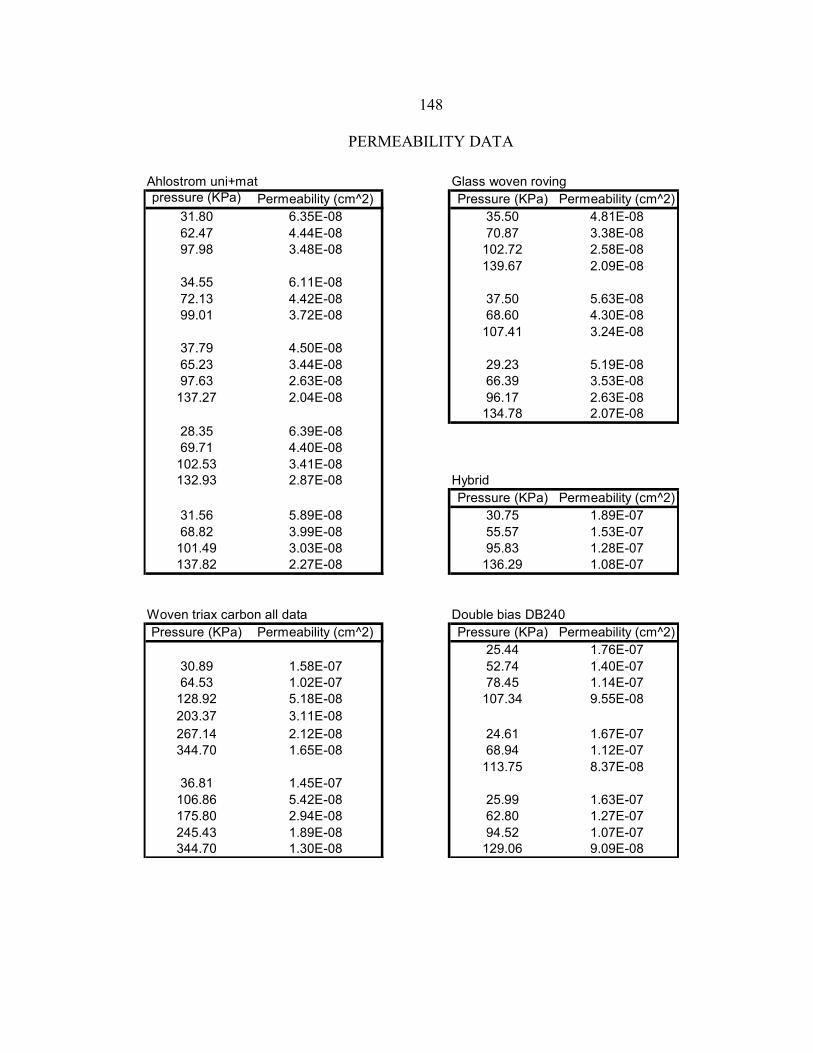
148
PERMEABILITY DATA
Ahlostrom uni+mat Glass woven rovingpressure (KPa) Permeability (cm^2) Pressure (KPa) Permeability (cm^2)
31.80 6.35E-08 35.50 4.81E-0862.47 4.44E-08 70.87 3.38E-0897.98 3.48E-08 102.72 2.58E-08
139.67 2.09E-0834.55 6.11E-0872.13 4.42E-08 37.50 5.63E-0899.01 3.72E-08 68.60 4.30E-08
107.41 3.24E-0837.79 4.50E-0865.23 3.44E-08 29.23 5.19E-0897.63 2.63E-08 66.39 3.53E-08
137.27 2.04E-08 96.17 2.63E-08134.78 2.07E-08
28.35 6.39E-0869.71 4.40E-08
102.53 3.41E-08132.93 2.87E-08 Hybrid
Pressure (KPa) Permeability (cm^2)31.56 5.89E-08 30.75 1.89E-0768.82 3.99E-08 55.57 1.53E-07
101.49 3.03E-08 95.83 1.28E-07137.82 2.27E-08 136.29 1.08E-07
Woven triax carbon all data Double bias DB240Pressure (KPa) Permeability (cm^2) Pressure (KPa) Permeability (cm^2)
25.44 1.76E-0730.89 1.58E-07 52.74 1.40E-0764.53 1.02E-07 78.45 1.14E-07
128.92 5.18E-08 107.34 9.55E-08203.37 3.11E-08267.14 2.12E-08 24.61 1.67E-07344.70 1.65E-08 68.94 1.12E-07
113.75 8.37E-0836.81 1.45E-07
106.86 5.42E-08 25.99 1.63E-07175.80 2.94E-08 62.80 1.27E-07245.43 1.89E-08 94.52 1.07E-07344.70 1.30E-08 129.06 9.09E-08

149
APPENDIX D
COMPACTION DATA

150
COMPACTION DATA
DB240 three plies Ahlostrom, 0 plus mat = 42024L/M50, 1250 g/m^2
Pressure (kPa)
Ply thickness (mm)
Fiber volume %
Thickness fraction
Pressure (kPa)
Ply thickness (mm)
Fiber volume %
Thickness fraction
0.84 1.06 28.98 1.00 0.844463 1.15 43.791.93 0.97 31.59 1.00 1.934031 1.0625 47.3921 14.70 0.87 35.03 0.90 4.700845 1.0425 48.3013 0.9811765.76 0.84 36.53 0.87 5.763796 1.0225 49.24607 0.9623537.81 0.82 37.16 0.85 7.812721 1.02 49.36677 0.969.72 0.77 39.95 0.79 9.718029 1.0025 50.22854 0.943529
11.60 0.76 40.52 0.78 11.60419 0.99 50.86274 0.93176513.60 0.71 42.99 0.74 13.59567 0.975 51.64524 0.91764713.60 0.71 43.14 0.73 13.59646 0.96 52.4522 0.90352919.44 0.70 43.92 0.72 19.43606 0.94 53.5682 0.88470629.15 0.69 44.23 0.71 29.15409 0.92 54.73273 0.86588238.87 0.67 45.55 0.69 38.87211 0.9 55.94901 0.84705948.59 0.60 51.20 0.62 48.59014 0.87 57.87829 0.81882471.44 0.59 52.15 0.61 71.43658 0.8325 60.48542 0.783529
0/90 rovingfiberglast #223 roving, 18 oz/yd^2, balanced weavetwo plies
Pressure (kPa)
Ply thickness (mm)
Fiber volume %
Thickness fraction
0.844463 0.7 33.74 11.934031 0.6 39.90667 14.700845 0.5575 42.94888 0.929166675.763796 0.51375 46.60633 0.856257.812721 0.50625 47.29679 0.843759.718029 0.505 47.41386 0.8416666711.60419 0.505 47.41386 0.8416666713.59567 0.505 47.41386 0.8416666713.59646 0.50125 47.76858 0.8354166719.43606 0.49 48.86531 0.8166666729.15409 0.48875 48.99028 0.8145833338.87211 0.43125 55.52232 0.7187548.59014 0.415 57.69639 0.6916666771.43658 0.405 59.12099 0.675

151
APPENDIX E
INPUT TO MODEL FOR EXPERIMENTAL CORRELATIONS

152
INPUT TO MODEL FOR EXPERIMENTAL CORRELATIONS
Test 1: Ahlstrom uni+mat fabric final_cm(1.31E-4,100,7.62, .9525, 13.21, 180, .2, 93, 2.923, .00132,.00003) permeability of the fabric K_f = inline('(2.02*10^-10 * P^2 - 6.7*10^-9 * P + 7.82*10^-8)') ply thickness fraction Tf = inline('(-.0631*log((P+.001)*10) + 1.073)') e = .5 Pcap = .4 Test 2: Ahlstrom uni+mat fabric final_cm(1.31E-4,100,8.89, 1.27, 13.21, 180, .32, 93, 2.90, .00132,.0000335) permeability of the fabric K_f = inline('(2.02*10^-10 * P^2 - 6.7*10^-9 * P + 7.82*10^-8)') ply thickness fraction Tf = inline('(-.0631*log((P+.001)*10) + 1.073)') e = .5 Pcap = .4
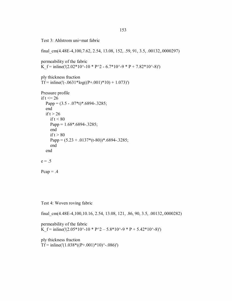
153
Test 3: Ahlstrom uni+mat fabric final_cm(4.48E-4,100,7.62, 2.54, 13.08, 152, .59, 91, 3.5, .00132,.0000297) permeability of the fabric K_f = inline('(2.02*10^-10 * P^2 - 6.7*10^-9 * P + 7.82*10^-8)') ply thickness fraction Tf = inline('(-.0631*log((P+.001)*10) + 1.073)') Pressure profile if t <= 26 Papp = (3.5 - .07*t)*.6894-.3285; end if t > 26 if t < 80 Papp = 1.68*.6894-.3285; end if t > 80 Papp = (5.23 + .0137*(t-80))*.6894-.3285; end end e = .5 Pcap = .4 Test 4: Woven roving fabric final_cm(4.48E-4,100,10.16, 2.54, 13.08, 121, .86, 90, 3.5, .00132,.0000282) permeability of the fabric K_f = inline('(2.05*10^-10 * P^2 – 5.8*10^-9 * P + 5.42*10^-8)') ply thickness fraction Tf = inline('(1.038*((P+.001)*10)^-.086)')

154
Pressure profile if t <= 45 Papp = 2.8235-.3285; end if t > 45 Papp = 2.8235+.0160*(t-45)-3.285; end if t >= 76 if t < 92 Papp = 1.0000-.3285; else Papp = 3.9000+.0032*(t-92)-.3285; end end V_inj = 2200 cm^3 e = .55 Pcap = .4
Related Documents