Simulating the water footprint of woodies in Aquacrop and Apex

Simulating the water footprintof woodies in Aquacrop and Apex

Mick Poppe

November 23, 2016

Master Thesis University of Twente

Water Engineering and Management

Title: Simulating the water footprint of woodies in Aquacrop and Apex

Author: Mick Poppe

Daily advisor: Ir. Joep F. Schyns

Head graduation committee: Dr. Ir. Martijn J. Booij

Date: November 23, 2016

Institution: University of Twente

Program: Civil engineering and management

Department: Water engineering and management

BE

GREEN

READ ON

SCREEN

Summary

As the crop cultivation sector is the largest human water consumer, models that simulate its wateruse are important in global water studies. Within this sector, herbaceous plants and woody plantscan be discriminated. Aquacrop is a plant simulation model very capable of simulating herbaceousplants, but the carry-over effects from one year to another, the large number of plant varieties and themore complicated evaporation and transpiration behaviour make the relative simple model not suitedfor the simulation of woodies. Apex is a model capable of simulating both herbaceous and woodyplants, but the constant that drives biomass growth changes over the seasons and locations and losesits linearity in stress conditions. This study compares the Aquacrop and Apex in the simulation ofwoody plants. For this the yield, the evapotranspiration and the water footprint resulting from theseare important.

From the plants with the largest harvested areas, the apple tree, the grapevine, the olive tree andthe oil palm are selected as four important plants that will be simulated in this study. Each of theseplants is simulated on a field level in the region where their core production is located. To make acomparison between the two very different models possible, the input and the processes in Aquacropand Apex are harmonized. To allow for a simulation of woody plants, Aquacrop only simulates theyearly foliage development of an already full-grown tree. Apex can simulate the plant developmentin the first years that characterize woodies.

For a full-grown woody plant, Aquacrop and Apex show different yields and evapotranspirationrates because of differences in input, parametrization and model structure. Aquacrop and Apex showroughly the same yield patterns in irrigated conditions, but in rainfed conditions large differences canoccur. The evapotranspiration rates are very similar in rainfed conditions, but in irrigated conditionsthey deviate a lot from each other. When we compare the yield with literature, both models ingeneral overestimate the yield. The evapotranspiration is in accordance with literature values.

The climatic variability influences the yields and evapotranspiration rates. In both models theevapotranspiration responds very realistically to yearly climate fluctuations. The yield in Aquacropalso responds as expected, but the yield in Apex is dominated by a model processes that does notcorrespond to the climatic variability. The influence of the soil is limited in Apex, while it can havea large effect on especially the yield in Aquacrop.

The development phase of woody plants is important for the lifelong average yields, because thefirst years of a plants life are characterized by a rather low yield. The evapotranspiration rate alsochanges over the first years, but the effect of the development phase is negligible for the lifelongaverage evapotranspiration. When we take the development of yield into account for the calculationof the water footprint, it becomes visible that the water footprints in irrigated conditions are quitesimilar between the models, while in rainfed conditions they can differ quite a lot because of thedifference in yield underlying the water footprint. Compared to the literature also large differencescan occur.

Both models show their limitations. Because of this, additional research is required to compare themodels under a wider scope. A case study can help to find more reliable estimates for the parametervalues in the models. From this study alone, it cannot be concluded that one model is better thananother. When simulating woodies, Aquacrop does not seem to be inferior to Apex, despite the factthat Aquacrop model is not designed for these plants.

3

Preface

A year ago I started working on my master thesis. The first few months where filled with the necessarypreparations. My goal was simple: contribute to the tree simulation part of the Aqua21 modellingframework. How? That is what I tried to find out during these months. With civil engineering as mybackground, I dived into literature unfamiliar to me. I wrote the chapters of the literature report,revised them, threw parts completely overboard and finally came up with the literature report meand my supervisors found satisfying. Parallel to this I also constructed a research proposal, andsimilar repetitions led to a final version of this too.

After finishing these two reports, I started working on the actual thesis. Diving into one model,a second one and even a third for some time, I slowly got familiar with the models. Slowly, as thispart took longer than expected. One model turned out to be unusable for the plans we had with it.A second one turned out to be difficult, because of the incomplete documentation and a complicatedmodel structure. A third one was quite workable, but not all results could be explained with thedocumentation provided. But day-by-day I got more trusted with the models and finally the daycame when I could produce results. Like a plant emerging from its seed, things started to develop.And not much later I’m writing this, as I finalized my project.

During the whole thesis my daily supervisor was Joep. Let me first say thank you. With thesame background as me, he sensed the difficulties I had with the models. Being well informed in bothmodels, he kept providing me with tips and answers for the questions I had. At the same time heshowed great dedication by taking his time for the feedback and helping me keep my focus on themain issues.

During the thesis and at the beginning of the preparations, Martijn was my final supervisor. Thankyou too. By taking his time for the feedback, with each typo and error noticed, he helped makingthe report much better. His general knowledge of the processes involved, while not having hand-onexperience with the models themselves, helped me more than once to get a better understanding ofthe processes underlying the models.

Most important, the feedback of Joep and Martijn completed each other. By focussing on thesame subject but having a different view on things, they helped getting the discussion going I neededto improve the study. For the feedback sessions, the phrase one plus one is three is truly applicable.I wish Joep all of luck with his PhD and his new born family. For Martijn nothing less of course. Ihope you again find the time to travel the world.

Besides Joep and Martijn, I have many others to thank. I like to thank Arjen with his help inthe preparation phase when Martijn was visiting New Zealand. I like to thank Abebe for sharing hisknowledge of Apex and helping me whenever I experienced problems with the model. Furthermore,I like to thank La and Hatem for sharing their knowledge of simulating woodies with Aquacrop.

MickNovember 23, 2016

4

Contents

1 Introduction 111.1 Background . . . . . . . . . . . . . . . . . . . . . . . . . . . . . . . . . . . . . . . . . . 111.2 State-of-the-art . . . . . . . . . . . . . . . . . . . . . . . . . . . . . . . . . . . . . . . . 121.3 Research gap . . . . . . . . . . . . . . . . . . . . . . . . . . . . . . . . . . . . . . . . . 131.4 Research goal and questions . . . . . . . . . . . . . . . . . . . . . . . . . . . . . . . . . 141.5 Reading guide . . . . . . . . . . . . . . . . . . . . . . . . . . . . . . . . . . . . . . . . . 14

2 Plant simulation models 152.1 General structure . . . . . . . . . . . . . . . . . . . . . . . . . . . . . . . . . . . . . . . 15

2.1.1 Plant simulation model vs. watershed simulation model . . . . . . . . . . . . . 162.1.2 Water-driven engine vs. solar-driven growth engine . . . . . . . . . . . . . . . . 16

2.2 Equations in the models . . . . . . . . . . . . . . . . . . . . . . . . . . . . . . . . . . . 182.2.1 Aquacrop . . . . . . . . . . . . . . . . . . . . . . . . . . . . . . . . . . . . . . . 182.2.2 Apex . . . . . . . . . . . . . . . . . . . . . . . . . . . . . . . . . . . . . . . . . . 22

3 Method 283.1 Plant selection & data collection . . . . . . . . . . . . . . . . . . . . . . . . . . . . . . 28

3.1.1 Plant selection . . . . . . . . . . . . . . . . . . . . . . . . . . . . . . . . . . . . 283.1.2 Location selection . . . . . . . . . . . . . . . . . . . . . . . . . . . . . . . . . . 303.1.3 Data collection . . . . . . . . . . . . . . . . . . . . . . . . . . . . . . . . . . . . 31

3.2 Model harmonization . . . . . . . . . . . . . . . . . . . . . . . . . . . . . . . . . . . . . 323.2.1 Input harmonization . . . . . . . . . . . . . . . . . . . . . . . . . . . . . . . . . 323.2.2 Harmonization of model processes . . . . . . . . . . . . . . . . . . . . . . . . . 32

3.3 Setting up Aquacrop for simulating woody plants . . . . . . . . . . . . . . . . . . . . . 333.4 Comparing the models . . . . . . . . . . . . . . . . . . . . . . . . . . . . . . . . . . . . 34

3.4.1 Average yield and evapotranspiration of full-grown plants . . . . . . . . . . . . 343.4.2 Environmental effects on the full-grown yield and evapotranspiration . . . . . . 353.4.3 The influence of plant development and the water footprint . . . . . . . . . . . 35

4 Results 374.1 Average yield and evapotranspiration of full-grown plants . . . . . . . . . . . . . . . . 37

4.1.1 Average yields . . . . . . . . . . . . . . . . . . . . . . . . . . . . . . . . . . . . 374.1.2 Average evapotranspiration rates . . . . . . . . . . . . . . . . . . . . . . . . . . 394.1.3 Concluding . . . . . . . . . . . . . . . . . . . . . . . . . . . . . . . . . . . . . . 40

4.2 Environmental effects on the full-grown yield and evapotranspiration . . . . . . . . . . 404.2.1 Climatic variability . . . . . . . . . . . . . . . . . . . . . . . . . . . . . . . . . . 404.2.2 Influence of soils . . . . . . . . . . . . . . . . . . . . . . . . . . . . . . . . . . . 434.2.3 Concluding . . . . . . . . . . . . . . . . . . . . . . . . . . . . . . . . . . . . . . 44

4.3 The influence of plant development and the water footprint . . . . . . . . . . . . . . . 44

5 Discussion 485.1 The performance of woodies in Aquacrop and Apex . . . . . . . . . . . . . . . . . . . 485.2 Comparison of Aquacrop simulation with literature . . . . . . . . . . . . . . . . . . . . 495.3 Applicability of methods and results . . . . . . . . . . . . . . . . . . . . . . . . . . . . 49

5

6 Conclusions & recommendations 516.1 Conclusions . . . . . . . . . . . . . . . . . . . . . . . . . . . . . . . . . . . . . . . . . . 516.2 Recommendations . . . . . . . . . . . . . . . . . . . . . . . . . . . . . . . . . . . . . . 52

A Technical information 57A.1 Simulation background . . . . . . . . . . . . . . . . . . . . . . . . . . . . . . . . . . . . 58

A.1.1 Main principles . . . . . . . . . . . . . . . . . . . . . . . . . . . . . . . . . . . . 58A.1.2 Stress conditions . . . . . . . . . . . . . . . . . . . . . . . . . . . . . . . . . . . 59A.1.3 Model versions . . . . . . . . . . . . . . . . . . . . . . . . . . . . . . . . . . . . 59A.1.4 Steps required to reproduce results . . . . . . . . . . . . . . . . . . . . . . . . . 60

A.2 Setting up input . . . . . . . . . . . . . . . . . . . . . . . . . . . . . . . . . . . . . . . 60A.2.1 Climate data . . . . . . . . . . . . . . . . . . . . . . . . . . . . . . . . . . . . . 60A.2.2 Soil parametrization . . . . . . . . . . . . . . . . . . . . . . . . . . . . . . . . . 63

A.3 Model set-up . . . . . . . . . . . . . . . . . . . . . . . . . . . . . . . . . . . . . . . . . 66A.3.1 Aquacrop . . . . . . . . . . . . . . . . . . . . . . . . . . . . . . . . . . . . . . . 66A.3.2 Apex . . . . . . . . . . . . . . . . . . . . . . . . . . . . . . . . . . . . . . . . . . 70

A.4 Plant implementation . . . . . . . . . . . . . . . . . . . . . . . . . . . . . . . . . . . . 74A.4.1 Green-up and harvest dates . . . . . . . . . . . . . . . . . . . . . . . . . . . . . 75A.4.2 Additional information Aquacrop . . . . . . . . . . . . . . . . . . . . . . . . . . 76A.4.3 Additional information Apex . . . . . . . . . . . . . . . . . . . . . . . . . . . . 84A.4.4 Plant data . . . . . . . . . . . . . . . . . . . . . . . . . . . . . . . . . . . . . . . 87

B Evapotranspiration function 92B.1 Background . . . . . . . . . . . . . . . . . . . . . . . . . . . . . . . . . . . . . . . . . . 92B.2 Evapotranspiration functions . . . . . . . . . . . . . . . . . . . . . . . . . . . . . . . . 92

B.2.1 Calculation procedure . . . . . . . . . . . . . . . . . . . . . . . . . . . . . . . . 93B.2.2 Performance according to RMSE . . . . . . . . . . . . . . . . . . . . . . . . . . 93B.2.3 Visual performance . . . . . . . . . . . . . . . . . . . . . . . . . . . . . . . . . . 95B.2.4 Selecting a function . . . . . . . . . . . . . . . . . . . . . . . . . . . . . . . . . 96

C Location of plants 97C.1 Climate and soil maps . . . . . . . . . . . . . . . . . . . . . . . . . . . . . . . . . . . . 97C.2 Location selection per plant . . . . . . . . . . . . . . . . . . . . . . . . . . . . . . . . . 98

C.2.1 Apple tree . . . . . . . . . . . . . . . . . . . . . . . . . . . . . . . . . . . . . . . 99C.2.2 Grapevine . . . . . . . . . . . . . . . . . . . . . . . . . . . . . . . . . . . . . . . 99C.2.3 Olive tree . . . . . . . . . . . . . . . . . . . . . . . . . . . . . . . . . . . . . . . 99C.2.4 Oil palm . . . . . . . . . . . . . . . . . . . . . . . . . . . . . . . . . . . . . . . . 99

C.3 Reference yield and evapotranspiration . . . . . . . . . . . . . . . . . . . . . . . . . . . 101C.4 Additional soils for further analysis . . . . . . . . . . . . . . . . . . . . . . . . . . . . . 102

6

List of Figures

2.1 Input components of plant simulation models . . . . . . . . . . . . . . . . . . . . . . . 152.2 Simulation characteristics of Aquacrop and Apex . . . . . . . . . . . . . . . . . . . . . 162.3 Model structures of Aquacrop and Apex . . . . . . . . . . . . . . . . . . . . . . . . . . 172.4 Implementation of stresses in Aquacrop . . . . . . . . . . . . . . . . . . . . . . . . . . . 182.5 Components of soil water balance in Aquacrop . . . . . . . . . . . . . . . . . . . . . . . 192.6 Leaf development in Aquacrop . . . . . . . . . . . . . . . . . . . . . . . . . . . . . . . . 202.7 Components of soil water balance in Apex . . . . . . . . . . . . . . . . . . . . . . . . . 24

3.1 Overview of the chapter . . . . . . . . . . . . . . . . . . . . . . . . . . . . . . . . . . . 283.2 Classification of the important woody plants . . . . . . . . . . . . . . . . . . . . . . . . 293.3 Simulation locations for the plants . . . . . . . . . . . . . . . . . . . . . . . . . . . . . . 303.4 Temperature and precipitation per location . . . . . . . . . . . . . . . . . . . . . . . . . 313.5 The main simulation principles in Aquacrop . . . . . . . . . . . . . . . . . . . . . . . . 33

4.1 Average yields of full-grown plants . . . . . . . . . . . . . . . . . . . . . . . . . . . . . 384.2 Average evapotranspiration rates of full-grown plants . . . . . . . . . . . . . . . . . . . 394.3 Yield variability of full-grown plants . . . . . . . . . . . . . . . . . . . . . . . . . . . . . 414.4 Evapotranspiration variability of full-grown plants . . . . . . . . . . . . . . . . . . . . . 434.5 Yield and evapotranspiration development in Apex . . . . . . . . . . . . . . . . . . . . 454.6 Factors that relate lifelong results with full-grown results . . . . . . . . . . . . . . . . . 464.7 The water footprint of the plants . . . . . . . . . . . . . . . . . . . . . . . . . . . . . . 47

A.1 Overview of the appendix . . . . . . . . . . . . . . . . . . . . . . . . . . . . . . . . . . 57A.2 Herbacous vs. woody and annual vs. perennial . . . . . . . . . . . . . . . . . . . . . . . 58A.3 Example of a monthly weather file of Apex . . . . . . . . . . . . . . . . . . . . . . . . . 63A.4 Effect of heat units to emergence in Aquacrop . . . . . . . . . . . . . . . . . . . . . . . 68A.5 Effect of shape salinity relation in Aquacrop . . . . . . . . . . . . . . . . . . . . . . . . 69A.6 Example of different database files in Apex . . . . . . . . . . . . . . . . . . . . . . . . . 71A.7 Example of operation file for calculating PHU in Apex . . . . . . . . . . . . . . . . . . 75A.8 Canopy cover growth equations in Aquacrop . . . . . . . . . . . . . . . . . . . . . . . . 77A.9 Effect of winter canopy on evapotranspiration in Aquacrop . . . . . . . . . . . . . . . . 79A.10 Canopy cover and plant factor resemblance in Aquacrop . . . . . . . . . . . . . . . . . 80A.11 Effect of plant factor on canopy cover in Aquacrop . . . . . . . . . . . . . . . . . . . . 82A.12 Effect of CGC on canopy cover in Aquacrop . . . . . . . . . . . . . . . . . . . . . . . . 83A.13 Root development in Aquacrop . . . . . . . . . . . . . . . . . . . . . . . . . . . . . . . 83A.14 Effect of planting density on the biomass in Apex . . . . . . . . . . . . . . . . . . . . . 84A.15 Effect of time to maturity in Apex . . . . . . . . . . . . . . . . . . . . . . . . . . . . . . 85A.16 Example of project file and operation file for Shandong . . . . . . . . . . . . . . . . . . 91

B.1 Performance of evapotranspiration functions . . . . . . . . . . . . . . . . . . . . . . . . 94B.2 Relation between evapotranspiration and mean solar radiation . . . . . . . . . . . . . . 95

C.1 The soil map used for location selection . . . . . . . . . . . . . . . . . . . . . . . . . . . 97C.2 The climate map used for location selection . . . . . . . . . . . . . . . . . . . . . . . . 98C.3 Global maps showing plant locations . . . . . . . . . . . . . . . . . . . . . . . . . . . . 101

7

List of Tables

3.1 Woody plants with the largest harvested areas . . . . . . . . . . . . . . . . . . . . . . . 293.2 Simulation locations per plant . . . . . . . . . . . . . . . . . . . . . . . . . . . . . . . . 303.3 Input data and their source . . . . . . . . . . . . . . . . . . . . . . . . . . . . . . . . . 323.4 Full-grown period of the plants . . . . . . . . . . . . . . . . . . . . . . . . . . . . . . . . 34

4.1 Overview of the full-grown yield and evapotranspiration . . . . . . . . . . . . . . . . . 404.2 Influence of soils on the yield and evapotranspiration . . . . . . . . . . . . . . . . . . . 444.3 Overview of the variability of the yield and evapotranspiration . . . . . . . . . . . . . . 44

A.1 Stresses in the models . . . . . . . . . . . . . . . . . . . . . . . . . . . . . . . . . . . . . 59A.2 Average monthly climate variables per location . . . . . . . . . . . . . . . . . . . . . . 61A.3 Carbon dioxide concentrations over the years . . . . . . . . . . . . . . . . . . . . . . . . 62A.4 Soil types per location . . . . . . . . . . . . . . . . . . . . . . . . . . . . . . . . . . . . 64A.5 Important soil parameters in Aquacrop . . . . . . . . . . . . . . . . . . . . . . . . . . . 64A.6 Soil parameters in Apex . . . . . . . . . . . . . . . . . . . . . . . . . . . . . . . . . . . 65A.7 Parametrization of Aquacrop files . . . . . . . . . . . . . . . . . . . . . . . . . . . . . . 68A.8 Parametrization Apex files . . . . . . . . . . . . . . . . . . . . . . . . . . . . . . . . . . 74A.9 The green-up dates and potential heat units for the plants . . . . . . . . . . . . . . . . 75A.10 The harvest dates for the plants . . . . . . . . . . . . . . . . . . . . . . . . . . . . . . . 76A.11 Relative weight foliage to aboveground biomass . . . . . . . . . . . . . . . . . . . . . . 78A.12 Aquacrop plant factors and growing stage lengths . . . . . . . . . . . . . . . . . . . . . 82A.13 Important plant parameters Apex . . . . . . . . . . . . . . . . . . . . . . . . . . . . . . 84A.14 The oil palm parameters for Apex . . . . . . . . . . . . . . . . . . . . . . . . . . . . . . 86A.15 Method to determine parameter values . . . . . . . . . . . . . . . . . . . . . . . . . . . 88A.16 Overview parameter values . . . . . . . . . . . . . . . . . . . . . . . . . . . . . . . . . . 89

B.1 RMSE of ET functions for all simulation locations . . . . . . . . . . . . . . . . . . . . . 95

C.1 The locations and their properties . . . . . . . . . . . . . . . . . . . . . . . . . . . . . . 99C.2 Literature yield and evapotranspiration . . . . . . . . . . . . . . . . . . . . . . . . . . . 102

8

List of Symbols

symbol (Apex) (Aquacr.) description unitClimatic inputCO2 CO2 Ca Atmospheric CO2 conc. [ppm]ET o - ETo Reference evapotranspiration [mm]P r P Precipitation [mm]Rsol RA - Solar radiation [MJ/m2]Tmin TMN Tn Min. temperature [◦C]Tmax TMX Tx Max. temperature [◦C]Soil input∆z DZ ∆z Thickness of soil layer [m]θfc FC θFC Water content at field capacity [m3/m3]θsat - θSAT Water content at saturation [m3/m3]θwp WP θWP Water content at wilting point [m3/m3]cn CN CN Curve number [−]Ksat SC Ksat Saturated hydraulic conductivity [mm/day]po PO - Porosity [mm]Model parametersCC max - CCx Maximum canopy cover [m2/m2]CC o - CCo Initial canopy cover [m2/m2]CDC - CDC Canopy decline coefficient [◦C−1]CGC - CGC Canopy growth coefficient [◦C−1]HU max - maturity Max. amount of heat units for a plant [◦C]HU sen - senescence Acc. heat units where senescense starts [◦C]HUI sen HUID - HUI when senescence occurs [◦C/◦C]ke,max - Kex Maximum evaporation rate [−]ktr,max - KcTr,x Maximum transpiration rate [−]Kmachine HE - HI reduction for machine efficiency [−]Kpest PSTF - HI reduction for pests [−]LAI max XLAI - Maximum leaf area index [m2/m2]LDC ad - Leaf decline coefficient [−]LGC 1 ah1 - First leaf growth coefficient [−]LGC 2 ah2 - Second leaf growth coefficient [−]PHU PHU - Potential heat units [◦C]rd1 ar1 - First rooting parameter [−]rd2 ar2 - Second rooting parameter [−]Tbase TBSC Tbase Lower boundary of plant T range [◦C]Tupper - Tupper Upper boundary of plant T range [◦C]Model variablesθ ST θ Soil moisture content [m3/m3]Broot RW - Root biomass [ton/ha]Bst STL B Standing (aboveground) biomass [ton/ha]Btotal DM - Total biomass [ton/ha]CC - CC Canopy cover [m2/m2]CC ∗ - CC∗ Adjusted canopy cover [m2/m2]

9

symbol (Apex) (Aquacr.) description unitCDC ws - CDCadj Canopy decline coefficient in water stress [◦C−1]CGC ws - CGCadj Canopy growth coefficient in water stress [◦C−1]E - E Evaporation [mm]ET p EO - Potential evapotranspiration [mm]Fperc QV D Percolation or drainage [mm]Fro Q RO Surface runoff [mm]Fuf UF CR Upward flow or capillary rise [mm]HI ∗ HIA HIadj Adjusted harvest index [−]HU HU GDD Heat units (or growing degree days) [◦C]HU sum - t Accumulated amount of heat units [◦C]HUI HUI - Heat unit index [◦C/◦C]ktr - KcTrx,sen Transpiration coefficient [−]Kage - KcTrx,adj Ageing correction on transpiration coef. [−]Kcold FTM - Dormancy factor temperature [−]Kday FHR - Dormancy factor daylength [−]Khi - fHI Adjustment factor for harvest index [−]Kpol - Kspol Adjustment for pollination [−]Ksen - fsen Sen. correction on transpiration coef. [−]Kws,ante - fante Adjustment water stress before yield [−]Kws,post - fpost Adjustment water stress after yield [−]LAI LAI - Leaf area index [m2/m2]Pi RFI - Amount of intercepted precipitation [mm]Pi,max RIMX - Max. amount of intercepted precipitation [mm]PAR PAR - Intercepted photosynthetic radiation [MJ/m2]RUE RUE - Radiation use efficiency [kg/ha · (MJ/m2)−1]Sas AS - Aeration stress coefficient [−]Sbiomass - Ksb Stress factor on biomass [−]Scdc - Kssen Stress factor on CDC [−]Scgc - Ksexp,w Stress factor on CGC [−]Se - Kr Stress factor on evaporation [−]Smin REG - Minimum stress factor [−]Sroot RGF - Minimum stress factor for roots [−]Sstrength SS - Root soil strength stress [−]Str,aer - Ksaer Aeration stress on transpiration [−]Sts,root ATS - Root temperature stress [−]Str,sto - Kssto Stomatal closure stress on transpiration [−]Sts TS - Temperature stress coefficient [−]Sws WS - Water stress factor [−]Tr UW Tr Transpiration [mm]Trp EP - Potential transpiration [mm]wt T - Water tension [kPa]WP∗ - WP∗ Adjusted water productivity [ton/ha]Y YLD Y Yield [ton/ha]

10

Chapter 1

Introduction

This study compares the simulations of woody plants in the plant simulation models Aquacrop andApex in the context of the water footprint. The meaning of this will become clear in this chapter.

1.1 Background

One of the main building blocks for a functioning human society is freshwater. Freshwater is usedfor drinking purposes, in industrial processes and for agricultural production. While freshwater isa renewable resource, it is finite. This means that at a certain location during a certain time theamount of freshwater is restrictive (Hoekstra and Mekonnen, 2011). Because of the many humanfunctions for freshwater, in combination with the natural demand in a watershed, the distribution ofthis limited amount of freshwater is a complex puzzle.

From the total human freshwater consumption, 85 percent comes at the account of the agricul-tural sector (Shiklomanov , 2000; Hoekstra and Chapagain, 2007). Within the agricultural sector, thecrop cultivation system and the livestock system can be discriminated. As 98 percent of the waterconsumption in the livestock system comes from the crop cultivation system in the form of food forlivestock, the crop cultivation system is by far the most important sector when it comes to water con-sumption (Mekonnen and Hoekstra, 2012). In the crop cultivation system two types of plants can bediscriminated, namely herbaceous plants and non-herbaceous, or woody, plants. All non-herbaceousplants, which are the trees and the shrubs, are perennial, while herbaceous plants can be both annualand perennial.

With the growing global population, the already high water demand from the agricultural sectorwill most likely increase considerably to meet the human food requirements (Doll and Siebert , 2002).However, the expected increasing demand from industry, electricity production and domestic usewill leave little room for a higher water consumption of agriculture. And water users are alreadycompeting for the available freshwater. To deal with these increasing conflicting water demands,descent water management is required to limit the consequences (OECD , 2012). Global studies thattrace water dependencies, water supplies and water demands can help to lay open vulnerabilities inthese complex water dynamics. This study is conducted in the context of the Aqua21 modellingframework, a study that will combine global hydrology and water footprints to identify locations ofwater stress and to identify patterns in water consumption.

The water footprint in the Aqua21 modelling framework follows the line of the ecological footprint,and indicates both the direct and indirect water use of a country, product, consumer or any otherstudy subject (Hoekstra and Hung , 2002; Chapagain and Hoekstra, 2004). In the agricultural sector,the water footprint of a crop is calculated by dividing the water consumption by the yield of theplant (Hoekstra et al., 2011). The water footprint is thus expressed in volume of water consumptionper unit of product. The water consumption of a plant is equal to the evapotranspiration duringthe growing season. For an annual plant, the water footprint can easily be calculated per year, asthe plant is sowed and harvested in the same year. For a perennial as a tree or shrub this is morecomprehensive, as the water footprint should be calculated from the yield and evapotranspirationover the complete life of the plant. This includes the first years of a plants life in which it is stilldeveloping its yield and years that the plant can be considered full-grown.

11

To calculate the water footprint of plants on a global scale, Aqua21 uses a plant simulationmodel. Such a model calculates the yield and evapotranspiration under the given environmental andmanagement conditions. The plant simulation model currently embedded in the modelling frameworkhas proved to be very capable of simulating herbaceous plants as wheat and maize under a wide rangeof conditions. How woody plants will be simulated within Aqua21 is not clear yet. This study istherefore concerned with the simulation of yield and evapotranspiration and the resulting waterfootprint for woody plants in a global context. While this is directly relevant for Aqua21, also otherglobal water studies that simulate woody plants benefit from this study.

1.2 State-of-the-art

Over the years many studies have used plant simulation models to simulate woody plants, often ona global scale. Plant simulation models can be classified according to their plant growth componentas either water-driven, solar-driven or carbon-driven (Steduto, 2006). In this first class, the plantgrowth is driven by the water consumption of the plant, while in the second class the plant growth isdriven by incoming solar radiation. The third class relates biomass growth directly with the carbonassimilation in the plant.

The water-driven models often use a method described by Allen et al. (1998) for the calculation ofthe evapotranspiration. Here the evapotranspiration is derived from a reference evapotranspiration,which is the evapotranspiration from a normalized surface. A model that incorporates the principlesof Allen et al. (1998) is Cropwat, a plant simulation model developed by the Food and AgricultureOrganization (FAO) of the United Nations. Hoekstra and Hung (2002) used this model to estimatevirtual water flows between countries and introduced with this the water footprint concept. Crop-wat calculated the evapotranspiration, while the yield in this study was retrieved from the Faostatdatabase. In the study 38 different plants were considered, including the woody plants oil palm,grapevine and citrus tree. Chapagain and Hoekstra (2004) continued on this study with a similarapproach for yield and evapotranspiration. However, this study was much more comprehensive andincluded 164 different plants, with a minority being woody plants. Mekonnen and Hoekstra (2011)simulated 146 different plants on a global scale and combined the Cropwat model with an own grid-based dynamic water balance model. This model also used the principles described by Allen et al.(1998). In this study the yields were not taken from a database, but were calculated by their ownmodel in order to account for processes as water stress. The model is a clear example of a water-drivenmodel, as the yield is directly linked with the evapotranspiration. These yields were scaled to nationaverage yields. Cropwat is still used these days in large-scale studies (for example Pfister and Bayer(2014)).

Doll and Siebert (2002) simulated irrigation water requirements on a global scale with the Water-gap model. This model was in its early stages capable of simulating two different types of plants; riceand nonrice. Watergap incorporated elements of Cropwat and calculated the irrigation requirementsbased on the evapotranspiration. The Watergap model has been used for multiple studies, amongthem a global water stress study to assess the impact of climate change (Alcamo et al., 2007). Siebertand Doll (2008) improved Watergap to a model called GCWN. This model shows remarkable simila-rities in parametrization with Cropwat. With this new model, 26 different plants were distinguished,including some woody plants. These days the Watergap model is still used for global grid-basedstudies (Schmied et al., 2016).

More recently, the Food and Agriculture Organization released a new plant simulation modelcalled Aquacrop. This model can be considered as the successor of Cropwat. At its basis also liethe principles of Allen et al. (1998). The model has been developed for the simulation of herbaceousplants, but is used for the simulation of woody plants as well. Hunink and Droogers (2010) andHunink and Droogers (2011) estimated the response of yield and water demand as a function ofclimate change. For Albania and Uzbekistan different plants were simulated, including the appletree, the grapevine and the olive tree. Zhuo et al. (2016) simulated yield and evapotranspirationin China. In this study Aquacrop has been used to simulate 17 plants, also including the appletree. Aquacrop is also the model currently embedded in the Aqua21 modelling framework for thecalculation of the water footprint for herbaceous plants.

Besides these water-driven models, also solar-driven models are used for grid-based simulations ofwoody plants. The most common used solar-driven model is Epic, a model that has been developed

12

for the simulation of soil productivity. The model Apex is an expansion of Epic, and allows forinteraction between different points in a grid-based analysis through the water balance. Both Apexand Epic are distributed by Texas A&M AgriLife Research. The models are capable of simulatingboth herbaceous and woody plants. Tan and Shibasaki (2003), Liu et al. (2009) and Balkovic et al.(2013) used Epic for the simulation of plants on a large scale. However, each of these studies onlysimulate herbaceous plants. This in contrast with Liu and Yang (2010), who used Epic for a globalsimulation and included a number of woody plants as grapevine, oil palm and citrus tree. The modelestimated the water consumption under both rainfed and irrigated conditions.

Next to the models based on Allen et al. (1998) and Apex and Epic, many other plant simulationmodels are found in literature. Often these models are solar-driven, such as Apsim (Keating et al.,2003), Dssat (Jones et al., 2003) and Stics (Brisson et al., 2003), sometimes they are carbon-drivenas Wofost (Supit et al., 1994) and sometimes models allow the user to select one of multiple growthengines, such as Cropsyst (Stockle et al., 2003). However, most of these models are not frequentlyused in global studies.

1.3 Research gap

There are many large scale studies concerned with the yield and evapotranspiration of woody plants.Carbon-driven models are not widely applied in global studies. The solar-driven models Apex andEpic are used in global studies and have the advantage to explicitly discriminate between herbaceousand woody plants. They take into account the different processes that characterize these plants,such as the fact that a tree does not die at harvest but simply loses a parts of its biomass tofruits. Unfortunately, these models have the disadvantage that the constant that relates the solarradiation with the biomass growth, the radiation use efficiency, changes during the seasons and overdifferent locations (Adam et al., 2011). Furthermore, this relation loses its linearity in stress conditions(Steduto, 2006). What remains are water-driven models as Cropwat, Watergap and Aquacrop, whichare indeed considered more stable under stress conditions (Steduto, 2006).

Aquacrop is the most recent water-driven model and is currently embedded in the Aqua21 model-ling framework for the simulation of herbaceous plants. This model has also been used in grid-basedstudies to simulate woody plants. However, Steduto et al. (2012) stated that the relative simplemodelling approach of Aquacrop make the model unsuitable for the simulation of woody plants. Thecarry-over effects from one year to another, the large number of plant varieties and the more com-plicated evaporation and transpiration behaviour cause complexities Aquacrop is not designed for.Current studies however do not take these complexities into account and treat woody plants as if theyare herbaceous. Woody plants are parametrised similarly as other plants and studies with Aquacropthus not discriminate between these two truly different kind of plants as Apex and Epic do. Alsothe other water-driven models Watergap and Cropwat apply the same simulation method to bothherbaceous and woody plants, despite their complicated structure.

Non of the models is capable of simulating woody plants while still having a reliable structureunder different conditions. Aquacrop is suppose to be stable under varying conditions but it doesnot discriminate between woody plants and herbaceous plants. Apex, which is a more comprehensivemodel than its sister model Epic, does discriminate between these different plant types, but suppose tobe less stable. However, a different model set-up might allow Aquacrop to simulate full-grown woodyplants, while Apex can simulate the development phase of the plants and might be more reliable thanliterature suggests. These two models will therefore be compared in this study for the simulation ofwoody plants as these two models are the most promising options for simulating woodies. As we arehere concerned with studies on a global scale, it is important to analyse the response of the modelsto different conditions. Unexpected responses on certain conditions can make a model unsuitable forsimulations in a global context.

For a woody plant a development period and a full-grown period can be distinguished. To calculatethe water footprint, the lifelong average yield and evapotranspiration should be known, as the waterfootprint is calculated from the complete life. As Aquacrop will only be able to simulate the full-grown period, the effect of this development period for the full simulation should be known. Apexcan simulate the development of the plant. By combining the results of the two models, the waterfootprint can be calculated for the full life of the plant.

Concluding, the water-driven model Aquacrop is currently used for the Aqua21 modelling frame-

13

work, but the more complex behaviour of woody plants can make it unsuitable for the simulationof woodies. However, a different set-up might allow for the simulations of full-grown woody plantswith Aquacrop. This can then be compared to Apex, which is already capable of simulating woodyplants. By comparing the models under various conditions, the performance of the models can beanalysed. To simulate the water footprint for these conditions, it is important that the influence ofthe development phase on the lifelong average yields and evapotranspiration rates is known.

1.4 Research goal and questions

The research goal of this study is directly derived from the research gap:

Compare the yields and evapotranspiration rates of full-grown woody plants simulatedwith AquaCrop and Apex under various environmental conditions, and subsequently cal-culate the water footprint of woodies, considering the influence of the development phaseon lifelong average yields and evapotranspiration rates.

The following research questions are asked with the goal:

1. What are the average yields and evapotranspiration rates of full-grown woody plants in themodels Aquacrop and Apex?

2. How do environmental conditions affect yields and evapotranspiration rates of full-grown woodyplants in Aquacrop and Apex?

3. What is the influence of the development phase on lifelong average yields and evapotranspirationrates and what is the resulting water footprint?

As there are many woody plants found all over the world and on top of this many cultivars, this studywill not be able to cover the full range of woody plants. This study will therefore focus on only fourimportant woody plants: the apple tree, the grapevine, the olive tree and the oil palm. The appletree is simulated at three different locations, the rest of the plants at only one location. The differentenvironmental conditions in this study are the climate and the soil. The total simulation period willbe limited by the amount of available data. All of these aspects are explained in detail later in thereport.

1.5 Reading guide

In chapter 2 the structure of the models, the underlying processes and the equations in the modelsare examined. Chapter 3 firstly explains the selection of interesting woodies and the collection ofthe corresponding data. This chapter also explains the method to simulate full-grown woody plantswith Aquacrop and provides information on how a fair comparison between the models is done.Also the method is presented to answer each of the research questions. With this, the woodies canbe simulated. The simulated yields and evapotranspiration rates and the resulting water footprintfor Aquacrop and Apex are compared in chapter 4. In chapter 5 the methods and the models arediscussed. Finally, chapter 6 gives the conclusions and recommendations resulting from this study.

14

Chapter 2

Plant simulation models

In this chapter the two plant simulation models Aquacrop and Apex are analysed in order to geta better understanding of the models. In section 2.1 the general structure of the two models iscompared. Section 2.2 discusses the equations in the models. The model descriptions are based onthe documentation belonging to the models. For Aquacrop this is given by Raes et al. (2012) and forApex this is given by Williams et al. (2012). This study uses Aquacrop version 4 and Apex version1501 revision 1604.

2.1 General structure

Aquacrop is a daily plant simulation model with a water-driven plant growth engine. Apex, onthe other hand, is a daily watershed simulation model with a solar-driven growth engine. Thesetwo different principles, plant simulation model versus watershed simulation model and water-drivenengine versus solar-driven engine, are explained below. But first, the input components of the modelsare shortly discussed.

In figure 2.1 the different input components of Aquacrop and Apex are shown. The model itself canbe considered as a series of coupled equations that calculate the plant growth. It is the responsibilityof the user to provide all the necessary data and parameters for these equations. To start with,this input consists of the location characteristics. These are climatic variables as temperature andprecipitation, and soil characteristics as saturated hydraulic conductivity and soil depth. The modelsalso require program parameters to be set. These are the parameters that generally not change fordifferent plants or locations. Furthermore, the user provides a plant to the model, characterized by acertain combination of parameters. Finally, the model requires data that describes the managementof the plant. This management includes for example planting dates and irrigation information.

From these input components the model calculates the plant growth. From the resulting output,the yield and evapotranspiration are most important in this study, as they are required for the waterfootprint calculation.

Model

Program parameters

Location characteristics:Climatic input

Soil data

Plant characteristics

Management

Output:Yield

Evapotranspiration

Figure 2.1: The input components of the plant simulation models Aquacrop and Apex.

15

Single plant & soil Single plant & soil

(a) Aquacrop

Reservoirs& rivers Multiple plants, multiple soils Urban

(b) Apex

Figure 2.2: The simulation characteristics of Aquacrop and Apex. Aquacrop is a plant simulationmodel, capable of simulating on a field basis. Apex is a watershed simulator, with capabilities ofsimulating multiple watershed characteristics.

2.1.1 Plant simulation model vs. watershed simulation model

Aquacrop is a model developed by the Food and Agriculture Organization (FAO) of the UnitedNations. It is a plant simulation model, implying that it is developed specifically for the simulation ofplants and that it does not take into account processes that are not directly related to plant growth.Apex, short for Agricultural Policy/Environmental eXtender, is distributed by Texas A&M AgriLifeResearch and is a watershed simulation model. This means that it is capable of simulating manydifferent characteristics of a watershed, such as rivers, reservoirs, different soils, different plants andurban areas. The difference between the two is visualized in figure 2.2.

Being only a plant simulation model, Aquacrop is rather simple and can only simulate on a so-called field level. This means that the model can only do point simulations; only one plant andone underlying soil structure can be simulated in a single simulation run. To simulate an area withdifferent plants and soil types, each of the different combinations should be simulated separately.There is no communication between the different simulation points. This can also be seen in figure2.2a.

Where Aquacrop can only simulate on a field level, Apex is capable of simulating on a watershedlevel. Besides the fact that this opens the possibility to simulate the previously mentioned reservoirs,urban areas and more, this also implies that the model can simulate multiple plants and soil combi-nations within a single run. In this case Apex can be seen as a coupled-field model, as there are stilldifferent fields where plant growth takes place. However, these different fields communicate to each,the communication lines being the water fluxes in Apex. This opens the possibility to make a morerealistic simulation of a composed area, but has the downside of a more complex model structure.

2.1.2 Water-driven engine vs. solar-driven growth engine

When we look at the growth engines of the simulation models, in this case Aquacrop and Apex but itis also applicable to other plant growth models, there are a few processes that can be found in bothmodels. See figure 2.3. First of all leaf development is simulated, mainly driven by the temperature.There are growth limitations depending on the availability of building material, in this case onlywater as nutrients are not considered in this study. With leaves on the plant, the plant will start totranspire and with this the evapotranspiration is affected. The biomass growth depends on the typeof model; in water-driven models this growth is a function of the water use of the plant, which is thetranspiration. In solar-driven models it depends on the solar radiation reaching the plant. From thisbiomass a certain yield can be derived.

Let us see how this is implemented in each of the models. The structure of Aquacrop is found infigure 2.3a. The leaf development in the model is indeed driven by temperature, with water stressinfluencing the growth. From this leaf development, the evaporation and transpiration are calculated,together forming the evapotranspiration. Both of them depend on the input variable reference eva-potranspiration, which is evapotranspiration from a normalized surface, forced by the local climateconditions. Also, the amount of water available influences the evaporation and transpiration. Ascan be seen in the figure, the biomass in Aquacrop is derived from the transpiration, from which itbecomes, by definition, a water-driven model. The carbon dioxide concentration in the atmosphereinfluences, together with the temperature, the biomass accumulation. From this biomass, the yieldis derived, affected by the temperature conditions and the water availability.

In Apex, the leaf development is also a function of the temperature and the water availability.This leaf development influences the biomass growth, but the biomass growth is also affected by thetemperature, water availability, carbon dioxide and, very important, the solar radiation. It is this

16

last one that makes Apex a solar-driven model. Note that Apex firstly calculates the total biomass(root weight plus aboveground weight), from which the aboveground biomass, or standing biomass,is derived. Parallel to this the temperature determines the potential amount of evapotranspirationthat can take place. These three components, being leaf development, biomass growth and poten-tial evapotranspiration, together determine the amount of evaporation and transpiration. From thestanding biomass, the yield can be derived, which depends on, among others, the transpiration.

Input Stresses Plant processes

Temperature

Precipitation/irrigation Water stressLeaf development

Reference ET

Precipitation/irrigation Water stressEvaporation

Reference ET

Precipitation/irrigation Water stress

Ageing/early senesc.

Transpiration

Evapotranspiration

Carbon dioxide

Temperature Temperature stressBiomass


Temperature Temperature stressYield

(a) Aquacrop

Input Stresses Plant processes

Temperature

Temperature Temperature stress


Leaf development

Temperature Potential ET

Carbon dioxide

Solar radiation

Temperature

Temperature Temperature stress


Total biomass

Evaporation

Transpiration

Evapotranspiration

Temperature Standing biomass

Temperature Yield

(b) Apex

Figure 2.3: The model structures of Aquacrop and Apex. Aquacrop is water-driven, as the biomass isa function of the transpiration. Apex is solar-driven, as the biomass is affected by the solar radation.See the text for a more detailed explanation of the models.

17

2.2 Equations in the models

With this general structure of the models in mind, we take a closer look at the equations in themodels. Below, Aquacrop and Apex are discussed separately.

2.2.1 Aquacrop

Aquacrop has a relatively simple model structure compared to Apex, caused by the fact that itonly simulates plants and not a whole watershed. Here we focus only on the simulation componentsimportant for this study. To be able to simulate plant growth, the model requires the climaticvariables daily minimum temperature (Tmin), daily maximum temperature (Tmax), daily precipitation(P ), daily reference evapotranspiration (ET o) and yearly atmospheric carbon dioxide concentrations(CO2). For the soil profile, the most important parameters are the water content at saturation (θsat),the water content at field capacity (θfc), the water content at wilting point (θwp) and the saturatedhydraulic conductivity (Ksat).

While having a relatively simple structure, Aquacrop is rather physical based resulting in a morecomplex simulation of processes compared to Apex. This is especially visible in the simulation ofstresses. Water stress, for example, is not implemented in the model as one stress coefficient, buthas many forms. While the application of water stress and other stresses will become clear in theexplanation of the different model components, the general principle of stresses in Aquacrop is similarfor all of them, see figure 2.4. In Aquacrop, the stress is simulated by a relative stress. If the modelsimulates water stress, plant parameters state at which water content water stress occurs and alsostate at which content the stress has reached its maximum. Within this range, the relative stress goesfrom zero to one. The value of the stress coefficient, the parameter actually applied in the model tosimulate the stress, is related to this relative stress in a linear, convex or logistic way.

In Aquacrop, a certain growth stage occurs at a certain amount of accumulated heat units (orgrowing degree days). Each plant has, depending on its parameters, a certain temperature rangethat it flourishes best in. When the temperature is above a plants minimum threshold, the additionaldegrees are stored as heat units. In equation form this looks like

HU (i) =Tmax(i) + Tmin(i)

2− Tbase; 0 ≤ HU (i) ≤ Tupper − Tbase, (2.1)

in which HU (i) [◦C] are the heat units acquired on day i, (Tmax(i)+Tmin(i))/2 is the mean temperatureon day i, based on the maximum temperature Tmax(i) [◦C] and the minimum temperature Tmin(i)[◦C]. Furthermore, Tupper [◦C] and Tbase [◦C] are plant properties describing the upper and lowerboundary of the temperature range. From this, the accumulated amount of heat units are calculatedwith

HU sum(i) =

n=i∑n=0

HU (n) HU sum(i) ≤ HU max, (2.2)

where HU sum(i) [◦C] is the accumulated amount of heat units on day i and HU max [◦C] is a plantproperty that describes the maximum amount of heat units that can be accumulated for the plant.When this number of accumulated heat units is reached, the life of a plant is complete.

Str

ess

coeffi

cie

nt

Relative stress

0 1

1

0

Linear shaped stress

Convex shaped stress

Logistic shaped stress

Figure 2.4: The general implementation of stress coefficients in Aquacrop.

18

layer 1

layer 2

Precipitation& irrigation

Runoff

EvaporationTranspiration

Percolation

Deeppercolation

Figure 2.5: The components present in the soil water balance of Aquacrop.

Soil-water balance

The soil-water balance is one of the main model components in Aquacrop. The water content in thisbalance determines the water stress, which is very important for the plant growth. An overview ofthe different components in the water balance is found in figure 2.5.

In Aquacrop, the soil profile is split into multiple layers. In each of the layers, a certain amount ofwater content can be calculated for the end of the day by taking the water content at the beginningof the day and calculating the remain of the ingoing and outgoing fluxes. Aquacrop starts with thecalculation of the outgoing flux percolation (or drainage). This is calculated by

Fperc(l, i) = f(Ksat(l), θfc(l), θsat(l),∆z(l), θ(l − 1, i− 1)), (2.3)

where Fperc(l, i) [mm] is the amount of percolation taking place from layer l on day i, Ksat(l)[mm/day] is the saturated hydraulic conductivity of layer l, θfc(l) [m3/m3] the field capacity oflayer l, θsat(l) [m3/m3] is the soil moisture content at saturation of the layer, ∆z(l) [m] is the thick-ness of the layer and θ(l − 1, i − 1) [m3/m3] the soil moisture content of the layer above layer l onthe beginning of day i.

After the calculation of the percolation, the ingoing flux infiltration is calculated. This is theirrigation, if applicable, and the precipitation minus a possible runoff. The runoff is calculated with

Fro(i) = f(cn, P (i)), (2.4)

where Fro(i) [mm] is the runoff on day i, cn [−] the curve number an P (i) [mm] the precipitation onday i. The infiltration water is distributed over the soil layers, depending on the maximum soil watercontent the layer accepts, the current soil water content and the saturated hydraulic conductivity.

With this updated amount of soil moisture content, the evaporation and transpiration are cal-culated. Evaporation occurs only from a small surface layer, while transpiration takes water fromthe root zone, which can cover the whole soil profile. More on evaporation and transpiration later.Aquacrop can also simulate capillary rise, but as there is no ground water table simulated in thisstudy, this capillary rise is always zero.

Leaf development

Aquacrop simulates leaf development as canopy cover, which is defined as the percentage of soil areathat is covered by the plant. The leaf development in the model is simulated by three equations; twothat describe the canopy incline at the beginning of the season and one that describes the canopydecline at the end of the season. For the canopy incline, one equation describes a concave incline,whereas the second one describes a convex incline. See figure 2.6. Furthermore, the canopy cover is

19

CC

time

incline (concave) incline (convex) decline

CCo

12CCmax

CCmax

HU sum to CCmax HU sum to HU sen HU sum to HUmax

Figure 2.6: The development of the canopy cover in Aquacrop.

influenced by stress. The three equations are

CC (i) =

CC o · eHU sum(i)·CGCws(i) if HU sum(i) ≤ HU sen & CC (i) ≤ 1

2CC max

CC max − 0.25 (CCmax)2

CCo· e−HU sum(i)·CGCws(i) if HU sum(i) ≤ HU sen & CC (i) > 1

2CC max

CC max · f(CDC ws(i),CC max) if HU sum(i) > HU sen,

(2.5)

where CC (i) [m2/m2] is the canopy cover on day i, CC o [m2/m2] and CC max [m2/m2] are plantproperties that describe the initial and maximum plant canopy cover, CGC ws(i) [◦C−1] and CDC ws(i)[◦C−1] are plant specific canopy growth and canopy decline parameters adjusted for water stress andHU sen [◦C] is a plant property that describes the amount of accumulated heat units required beforecanopy decline starts.

The effect of water stress on the canopy growth coefficient is calculated with

CGC ws(i) = Scgc(i) · CGC , (2.6)

in which CGC [◦C−1] is the plant parameter canopy growth coefficient and Scgc(i) [−] is the waterstress coefficient going from one (no water stress) to zero (maximum water stress). The water stressfor the canopy growth coefficient depends on two things. Firstly, it depends on the moisture contentin the soil, which is determined in the soil-water balance. Secondly, it depends on the sensitivity ofthe plant to water stress. Firstly the total amount of water the soil can hold is determined. This isa function of the water content at field capacity, the water content at wilting point and the rootingdepth. A certain fraction of this states the soil moisture content where the plant will start to feelthe stress (the point where the relative stress is zero). Another fraction, also a plant parameter,determines the content at which the stress is maximum (relative stress is one).

Water stress can also cause an early senescence of the plant. This is simulated in Aquacrop byan early canopy decline. Normally, the decline starts at the point where the accumulated heat unitshave reached the user specified amount of heat units at which senescence starts. Before this point,there is no canopy decline, i.e. the canopy decline coefficient is zero. To simulate early senescencedue to water stress, Aquacrop uses the equation

CDC ws(i) = (1− Scdc8(i)) · CDC , (2.7)

where CDC [◦C−1] is the plant parameter canopy decline coefficient and Scdc [−] is the water stresscoefficient for canopy decline. As can be seen in this equation, no water stress (stress coefficient isone) will result in no adjustment of the canopy decline coefficient. This means that no early declineoccurs. Comparable with the water stress effects on the growth coefficient, the stress depends on thewater availability and the sensitivity of the plant. The upper limit of the sensitivity is again specifiedby a plant specific parameter. The lower limit is equal to the wilting point.

Evapotranspiration

In Aquacrop, both evaporation and transpiration are governed by the reference evapotranspiration.Evaporation is determined by

E(i) = Se(i) · (1− CC ∗(i)) · ke,max · ET o(i), (2.8)

20

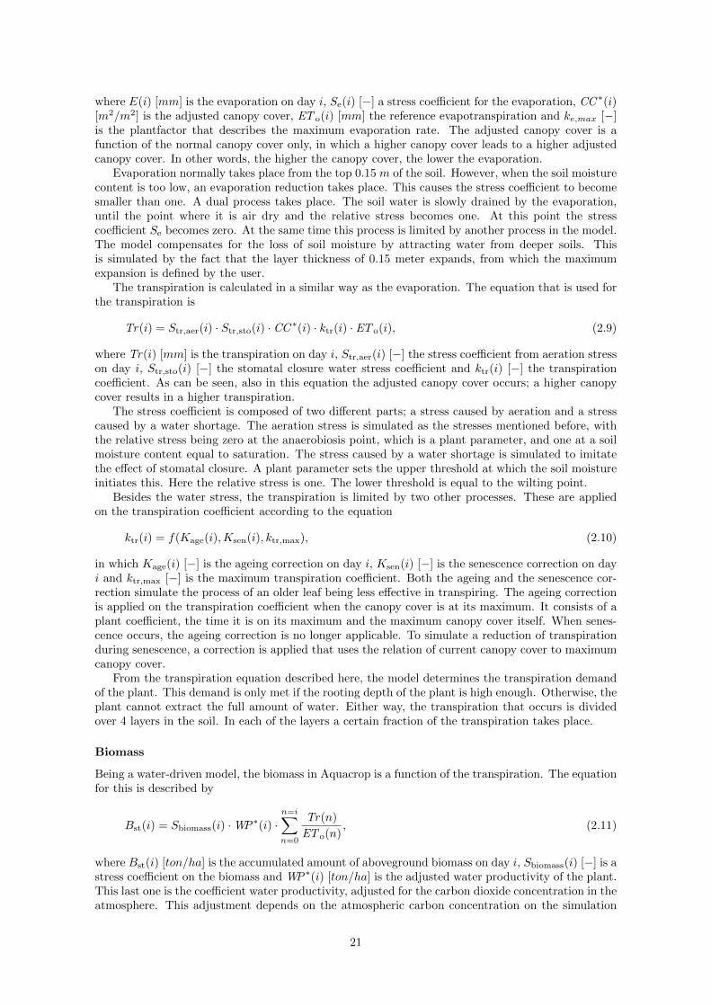
where E(i) [mm] is the evaporation on day i, Se(i) [−] a stress coefficient for the evaporation, CC ∗(i)[m2/m2] is the adjusted canopy cover, ET o(i) [mm] the reference evapotranspiration and ke,max [−]is the plantfactor that describes the maximum evaporation rate. The adjusted canopy cover is afunction of the normal canopy cover only, in which a higher canopy cover leads to a higher adjustedcanopy cover. In other words, the higher the canopy cover, the lower the evaporation.

Evaporation normally takes place from the top 0.15 m of the soil. However, when the soil moisturecontent is too low, an evaporation reduction takes place. This causes the stress coefficient to becomesmaller than one. A dual process takes place. The soil water is slowly drained by the evaporation,until the point where it is air dry and the relative stress becomes one. At this point the stresscoefficient Se becomes zero. At the same time this process is limited by another process in the model.The model compensates for the loss of soil moisture by attracting water from deeper soils. Thisis simulated by the fact that the layer thickness of 0.15 meter expands, from which the maximumexpansion is defined by the user.

The transpiration is calculated in a similar way as the evaporation. The equation that is used forthe transpiration is

Tr(i) = Str,aer(i) · Str,sto(i) · CC ∗(i) · ktr(i) · ET o(i), (2.9)

where Tr(i) [mm] is the transpiration on day i, Str,aer(i) [−] the stress coefficient from aeration stresson day i, Str,sto(i) [−] the stomatal closure water stress coefficient and ktr(i) [−] the transpirationcoefficient. As can be seen, also in this equation the adjusted canopy cover occurs; a higher canopycover results in a higher transpiration.

The stress coefficient is composed of two different parts; a stress caused by aeration and a stresscaused by a water shortage. The aeration stress is simulated as the stresses mentioned before, withthe relative stress being zero at the anaerobiosis point, which is a plant parameter, and one at a soilmoisture content equal to saturation. The stress caused by a water shortage is simulated to imitatethe effect of stomatal closure. A plant parameter sets the upper threshold at which the soil moistureinitiates this. Here the relative stress is one. The lower threshold is equal to the wilting point.

Besides the water stress, the transpiration is limited by two other processes. These are appliedon the transpiration coefficient according to the equation

ktr(i) = f(Kage(i),Ksen(i), ktr,max), (2.10)

in which Kage(i) [−] is the ageing correction on day i, Ksen(i) [−] is the senescence correction on dayi and ktr,max [−] is the maximum transpiration coefficient. Both the ageing and the senescence cor-rection simulate the process of an older leaf being less effective in transpiring. The ageing correctionis applied on the transpiration coefficient when the canopy cover is at its maximum. It consists of aplant coefficient, the time it is on its maximum and the maximum canopy cover itself. When senes-cence occurs, the ageing correction is no longer applicable. To simulate a reduction of transpirationduring senescence, a correction is applied that uses the relation of current canopy cover to maximumcanopy cover.

From the transpiration equation described here, the model determines the transpiration demandof the plant. This demand is only met if the rooting depth of the plant is high enough. Otherwise, theplant cannot extract the full amount of water. Either way, the transpiration that occurs is dividedover 4 layers in the soil. In each of the layers a certain fraction of the transpiration takes place.

Biomass

Being a water-driven model, the biomass in Aquacrop is a function of the transpiration. The equationfor this is described by

Bst(i) = Sbiomass(i) ·WP∗(i) ·n=i∑n=0

Tr(n)

ET o(n), (2.11)

where Bst(i) [ton/ha] is the accumulated amount of aboveground biomass on day i, Sbiomass(i) [−] is astress coefficient on the biomass and WP∗(i) [ton/ha] is the adjusted water productivity of the plant.This last one is the coefficient water productivity, adjusted for the carbon dioxide concentration in theatmosphere. This adjustment depends on the atmospheric carbon concentration on the simulation

21

day, a plant parameter that determines the sensitivity of a plant to the carbon concentration and anumber of program parameters that determine the relations with a reference concentration.

The stress coefficient for the biomass is a temperature stress. While a plant grows when the dailytemperature is above the minimum temperature the plant requires, the plant has also an optimaltemperature. The relative stress for the biomass is one when the temperature is exactly equal orlower than the minimum temperature. In this case the stress coefficient is zero and no biomass isaccumulated. When the temperature has reached its optimum temperature, the relative stress is zero.At temperatures higher than the optimum, this relative stress stays zero.

Yield

Finally, from this biomass the yield can be derived. This is done by the equation

Y (i) = Khi(i) ·HI ∗(i) ·Bst(i), (2.12)

in which Y (i) [ton/ha] is the yield on day i, Khi(i) [−] is an adjustment factor and HI ∗(i) [−] theadjusted harvest index. As can be seen, a larger biomass leads to a larger yield. The harvest indexis a plant specific parameter that, depending on the type of plant, grows according to a fixed growthcurve to its maximum value. However, it is adjusted when early senescence occurs. If the canopycover gets below a certain threshold, the program mimics the lack of photosynthesis by stopping theincrease of harvest index. When this occurs too early in the season, the harvest index might stay atzero.

The adjustment factor for the harvest index is composed of multiple items. In the model thisadjustment looks like

Khi = Kws,ante(i) ·Kpol(i) ·Kws,post(i), (2.13)

in which Kws,ante(i) [−] is the adjustment for water stress before the yield formation, Kpol(i) [−] theadjustment for pollination failure and Kws,post(i) [−] the adjustment for water stress during yieldformation. To start with the first one, the water stress before yield formation might cause an increaseof harvest index because the plant has not yet spent its energy on the growing of the biomass. Thesize of this increase depends on the fraction of actual biomass at the start of flowering relative to thefraction of potential biomass. The range at which this fraction will cause a positive adjustment ofthe harvest index depends on the maximum harvest index increase the user allows for.

The second adjustment, the adjustment for failure of pollination, is applied when the conditionsat the moment of flowering are such that the amount of flowers growing on the plant is not sufficientto grow the total amount of fruits. These severe conditions can be caused by water stress andtemperature stress. For the water stress, a similar pattern as before is visible, with a plant parameterdetermining at which water content the stress occurs. The lower limit is set at wilting point. Forthe temperature stress, both a cold stress and a heat stress can cause the pollination to fail. Twoplant parameters determine the minimum and maximum temperature for pollination. When the dailytemperature is below this minimum or above this maximum, pollination starts to fail. The relativestress is zero at these temperatures, and increases to one when the temperature goes to five degreesbelow the minimum or five degrees above the maximum. At this point, no flowers grow.

Finally, water stress might occur during the yield formation. When this water stress limits theexpansion of canopy, but does not limit the transpiration, this adjustment is positive. When thestress also limits the transpiration, the adjustment factor will become negative as the yield grows alsoless than optimal with such stress. In the equation of this adjustment, the stress coefficient limitingthe canopy growth coefficient in the leaf development (Scgc) is present for this first situation. For thesecond situation, when the transpiration is limited, the stress coefficient in the transpiration equation(Str,sto) is present.

2.2.2 Apex

Being a watershed simulator, Apex has a more complex structure than Aquacrop as it contains morecomponents. However, the processes themselves are not as physically based as Aquacrop, resulting ina simpler simulation of processes. This section will not discuss all simulation components; only thecomponents relevant for the yield and evapotranspiration are explained. Also, as will become clear

22

in chapter 3, Apex will be used on a field-level by making all the horizontal components in the soilwater balance zero. From the stresses, the fertility stress and the aluminum stress are not considered.These parts are therefore also left out of the description in this section.

To simulate with Apex, the model needs maximum and minimum daily temperatures (Tmax andTmin), daily precipitation (P ), mean daily solar radiation (Rsol) and yearly atmospheric carbon dioxideconcentrations (CO2). For the soil profile, the model requires much more parameters as Aquacropdid. The most important ones are the water content at field capacity (θfc), the water content atwilting point (θwp), the saturated hydraulic conductivity (Ksat) and the porosity (po). The rest ofthe soil parameters will be mentioned later.

The more simple simulation of processes in Apex is mainly visible in the simulation of stresses.Where Aquacrop has different stress coefficients for the different processes in the model, Apex ischaracterized by only two stress coefficients; one for the biomass of the roots and one for the remainingparts. This second one is composed of three components and looks like

Smin(i) = min(Sws(i), Sas(i), Sts(i)), (2.14)

in which Smin(i) [−] is the minimal stress coefficient on day i, Sws(i) [−] the water stress coefficient,Sas(i) [−] the aeration stress coefficient and Sts(i) [−] the temperature stress coefficient. As each ofthe three stress components can fluctuate between zero (full stress) and one (no stress), the minimalstress has the same range. The water stress coefficient is the actual transpiration divided by thepotential one. The aeration stress coefficient is a function of the current water content, the fieldcapacity and the porosity in the top soil layer and a plant parameter that states the sensitivity of theplant to aeration stress. Finally, the temperature stress is a function of the mean daily temperatureand two plant parameters describing the minimum and optimal growing temperature. The otherstress coefficient, the one for the roots, is described later.

In a similar way as Aquacrop, heat units are accumulated in Apex according to the function


2− Tbase; 0 ≤ HU (i). (2.15)

As can be seen, this is the same equation as Aquacrop uses, except that the number of heat unitacquired on a certain day is not limited by a maximum. In Apex, the acquired heat units are usedfor the heat unit index according to the equation

HUI (i) =1

PHU·n=i∑n=0

HU (n); HUI (i) ≤ 1, (2.16)

wherein HUI (i) [◦C/◦C] is the heat unit index on day i and PHU [◦C] is a plant property thatdescribes the heat units that are required before a plant is full-grown. The heat unit index is usedfor many different processes in the model. While the documentation states this simple equation forthe heat unit index, corrections on the heat unit index occur, for example at harvest and when theheat unit index reaches one. These corrections are not mentioned in the model documentation.

Soil-water balance

The soil-water balance in Apex is to a certain extent comparable with the one of Aquacrop. This iscaused by the fact that all horizontal components in the soil-water balance are set equal to zero. Ina number of soil layers, the soil-water balance is responsible for the water stress component in themodel as it can limit the amount of transpiration taking place. In figure 2.7 the soil-water balance isvisualized.

The input of water into the system is firstly given by the precipitation, which is partly interceptedby the standing plant. The intercepted precipitation is calculated with the equation

Pi(i) = f(Pi,max(i), Bst(i),LAI (i)), (2.17)

in which Pi(i) [mm] is the amount of intercepted precipitation on day i, Pi,max(i) [mm] is the maximumamount of precipitation that can be intercepted on day i and LAI (i) [m2/m2] the leaf development onday i (more on the LAI below). The maximum amount of precipitation that can be intercepted is notfurther explained in the documentation, but is most likely a function of at least the precipitation on

23

layer 1

layer 2

Precipitation Interceptedprecipitation

Runoff

EvaporationTranspiration Irrigation

Runoff

Percolation

Percolation

Upward flowBackpass

Backpass

Figure 2.7: The components present in the soil water balance of Apex.

the day considered. The remaining precipitation, thus the precipitation minus the intercepted part,reaches the soil.

When reaching the soil, the precipitation partly becomes runoff. Just as with Aquacrop this isbased on the curve number method. The equation for the runoff is

Fro(i) = f(cn, P (i)− Pi(i)). (2.18)

The curve number is not directly entered into the model, but is calculated indirectly by giving theland use number and the hydrologic soil group. The curve number is adjusted for the slope ofthe watershed. The remaining part of the precipitation, thus the original precipitation minus theintercepted part and the runoff part, adds to the soil-water balance. Besides this, also the irrigationwater adds to the soil-water balance. A certain fraction of the irrigation can become runoff, but inthis study this fraction is set to zero.

The water from the precipitation and irrigation will increase the water content in the layer. Atsome point, this water content will become larger than the field capacity, causing a flow from thelayer. While the model allows for a horizontal component as well, this study only considers a verticalflow. This vertical flow, or percolation, is calculated according to the equation

Fperc(l, i) = f(Ksat(l), θfc(l), po(l)), (2.19)

in which po [mm] is the soil porosity. Percolation occurs layer by layer, where the lowest layercontributes to the groundwater storage. The groundwater storage has no further interaction with theconsidered field; it only affects a possible downstream subarea.

Besides the vertical flow downwards, two upwards flows are present in the model. Firstly, there isa so-called backpass, which occurs in case of the physically impossible situation that the amount ofwater in a layer exceeds the porosity of that layer. This additional water is added to the above layer.In the highest layer, the water is transported out of the soil profile. Secondly, there is the upwardflow, or capillary rise, which occurs when a lower layer exceeds field capacity. This is calculatedaccording to

Fuf(l, i) = f(θfc(l), θwp(l),wt(i, l),wt(i, l − 1)), (2.20)

where Fuf(l, i) [mm] is the upward flow in layer l on day i and wt(i, l) [kPa] and wt(i, l − 1) [kPa]are the water tensions in the layer considered and the layer above. The water tension of a certainlayer is a function of the wilting point, the field capacity and the actual soil-moisture content. Thereis no upward flow into the lowest soil layer.

Besides these processes, also evaporation and transpiration influence the soil-water balance. Moreon these later.

24

Leaf development

In the soil-water balance, the leaf area index (LAI ) was already mentioned. This is a widely appliedleaf variable which is defined as the total area of leaves per area of soil. Both a leaf incline phase anda leaf decline phase are simulated, according to the equations

LAI (i) =

{f(LAI (i− 1),HUI (i), Smin(i),LAI max,LGC 1,LGC 2) if HUI (i) ≤ HUI sen

f(LAI (i− 1),HUI (i),HUI sen,LDC ) if HUI (i) > HUI sen,(2.21)

wherein LAI max [m2/m2] is the maximum leaf area index of a plant, LGC 1 [−] and LGC 2 [−] are twoplant parameters that link the heat unit index with the leaf development, LDC [−] is a leaf declineparameter and HUI sen [◦C/◦C] the heat unit index at which canopy decline is initiated.

Besides the decline phase of leaf area index, there is also a winter dormancy present in themodel. However, the interaction between the decline and the dormancy is not expanded on in thedocumentation. The equation for the dormancy looks like

LAI (i) = LAI (i− 1) · (1−max(Kday(i),Kcold(i))), (2.22)

in which Kday(i) [−] is a dormancy factor for the daylength and Kcold(i) [−] is a dormancy factor forthe temperature. The first one is a function of the latitude and the day of the year. This factor isonly considered when the daylength is within one hour of the shortest daylength. This factor is onewhen the daylength is equal to or larger than one hour above the shortest daylength. The dormancyfactor for temperature only applies when the minimum daily temperature is below -1 ◦C. It is afunction of this minimum daily temperature and two parameters that describe the sensitivity of aplant to this temperature.

Evapotranspiration

In Apex, some important parts of the evapotranspiration equations are documented unsatisfying.Therefore, the evapotranspiration process lets itself best be explained in words, with only a fewclarifying equations. While here the evapotranspiration functions according to the documentationare presented, differences were observed between these documented processes and the output of themodel.

The calculation of the potential evapotranspiration is rather straightforward, and is calculatedaccording to one of the five evapotranspiration functions. In this study, the Hargreaves function isused, which is a function of the daily minimum and maximum temperature and the maximum possiblesolar radiation. This last one is a function of the latitude and the day of the year.

Evaporation is composed of a few parts; evaporation from soil, evaporation of snow and evapo-ration from litter storage. The potential evapotranspiration is split over the transpiration and theevaporation from soil. When the amount of intercepted rain is larger than the potential evapotrans-piration, potential transpiration and potential evaporation from soil are zero on that day. When thisis not the case, the potential transpiration depends on the leaf area index; a larger leaf area indexresults in a higher amount of transpiration. Furthermore, the potential transpiration can never bemore than the potential evapotranspiration minus the intercepted precipitation. In equation thislooks like

Trp(i) = min(f(LAI(i)),ET p(i)− Pi(i)), (2.23)

in which Trp(i) [mm] it the potential transpiration and ET p(i) [mm] is the potential evapotranspi-ration.

The actual transpiration is derived from this potential one. Depending on some soil properties,such as the soil water content of a soil layer, the field capacity and the wilting point, and some rootproperties such as the rooting depth and the root stress factor, the water for the transpiration isextracted from different soil layers. A soil layer with a high water content can compensate for alayer with little water. However, this can only continue for so long and at some point the potentialtranspiration will be hampered.

To calculate the actual transpiration, the root stress factor is required. The equation for this is

Sroot(i) = min(Sts,root(i), Sstrength(i)), (2.24)

25

in which Sroot(i) [−] is the root stress factor on day i, Sts,root(i) [−] the temperature stress factor forthe roots and Sstrength(i) [−] the soil strength stress factor. The soil strength stress factor representsthe resistance of a soil to root growth, and is a function of the bulk density and the sand contentof the soil, both soil input parameters. The temperature stress factor for the roots is a soil layerspecific variable and depends on the soil temperature of a certain layer and the optimal and minimumtemperature of a plant. The soil temperature depends on the soil parameters depth of the layer, bulkdensity, albedo and water content, the plant biomass, the snow cover and the climatic variables dailyminimum and maximum temperature and mean daily radiation.

When the potential evapotranspiration is larger than the intercepted amount of precipitation,besides transpiration also soil evaporation can take place. The amount of this potential evaporationdepends on the amount of soil covered by the plants; a higher plant cover results in a lower potentialsoil evaporation. The plant cover is a function of the aboveground biomass and the leaf area index ofthe plant. The potential soil evaporation furthermore depends on the potential evapotranspirationand the part of this already distributed to potential transpiration.

The actual soil evaporation is derived from the potential soil evaporation depending on the watercontent, the field capacity and the wilting point of the first 0.5 meter of the soil. For the totalevaporation, first the snow, if present, will evaporate, followed by the litter storage. After this, soilevaporation will take place. Snow will probably be a function of the precipitation and the temperature,but its equation is not mentioned in the documentation. The litter storage consists of the interceptedprecipitation by the plant.

Biomass

In Apex, there are two different biomass components present; the root biomass and the abovegroundbiomass. As the yield is derived from the aboveground biomass, only this part is interesting here.However, the aboveground biomass is derived in three steps. First the total biomass, thus the above-ground biomass plus the root biomass is calculated. From this, the root biomass can be calculated.The aboveground biomass is then the total biomass minus the biomass of the roots.

As can be expected from a solar driven model, an important component in the biomass accumu-lation is the solar radiation. The equation for the total biomass is given by

Btotal(i) =

n=i∑n=0

0.001 · PAR(n) · (RUE (n)− f(Tmin(n), Tmax(n))) · Smin(n), (2.25)

where Btotal(i) [ton/ha] is the total biomass on day i, PAR(i) [MJ/m2] the intercepted photosyn-thetic radiation and RUE (i) [kg/ha · (MJ/m2)−1] the radiation use efficiency. The radiation useefficiency is a function of the atmospheric carbon dioxide concentration and some plant parametersthat represent the sensitivity of the plant to increasing carbon dioxide concentrations. The inter-cepted photosynthetic radiation is the radiation reaching the plant, which is a function of the meandaily solar radiation (Rsol), which is input, and the leaf area index.

The next step is to calculate the biomass of the roots. This is calculated with the equation

Broot(i) = f(Btotal(i),HUI (i), rd1, rd2), (2.26)

wherein Broot(i) [ton/ha] is the root biomass on day i and rd1 [−] and rd2 [−] are two plant parametersthat determine which fraction of total biomass goes towards the roots. The root biomass is distributedover different soil layers in the same fractions as the distribution of transpiration over the layers.

With the total biomass and the root biomass, the aboveground, or standing, biomass can easilybe calculated according

Bst(i) = Btotal(i)−Broot(i). (2.27)

The documentation also reports a dormancy influence on the standing biomass. This dormancyhas the same construction as the dormancy on the leaf area index, with a dormancy factor for thedaylength and a dormancy factor for the temperature.

26

Yield

Finally, the yield can be calculated with the standing biomass. The equation for the yield in Apex is

Y (i) = HI ∗(i) ·Kpest ·Kmachine ·Bst(i), (2.28)

wherein HI ∗(i) [−] is the adjusted harvest index, Kpest [−] a factor that reduces the yield becauseof pests and Kmachine [−] a reduction factor because of the harvest efficiency. The pest factor isa function of, among others, the sensitivity of the plant to pests. The adjusted harvest index isa function of the optimal and minimum harvest index, both plant properties, the heat unit index,which determines the growth from the minimum to the optimal harvest index, and the transpirationduring the part of the season where the harvest index increases most, which is often the last half ofthe season.

27

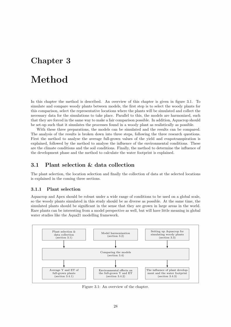
Chapter 3

Method

In this chapter the method is described. An overview of this chapter is given in figure 3.1. Tosimulate and compare woody plants between models, the first step is to select the woody plants forthis comparison, select the representative locations where the plants will be simulated and collect thenecessary data for the simulations to take place. Parallel to this, the models are harmonized, suchthat they are forced in the same way to make a fair comparison possible. In addition, Aquacrop shouldbe set-up such that it simulates the processes found in a woody plant as realistically as possible.

With these three preparations, the models can be simulated and the results can be compared.The analysis of the results is broken down into three steps, following the three research questions.First the method to analyse the average full-grown values of the yield and evapotranspiration isexplained, followed by the method to analyse the influence of the environmental conditions. Theseare the climate conditions and the soil conditions. Finally, the method to determine the influence ofthe development phase and the method to calculate the water footprint is explained.

3.1 Plant selection & data collection

The plant selection, the location selection and finally the collection of data at the selected locationsis explained in the coming three sections.

3.1.1 Plant selection

Aquacrop and Apex should be robust under a wide range of conditions to be used on a global scale,so the woody plants simulated in this study should be as diverse as possible. At the same time, thesimulated plants should be significant in the sense that they are grown in large areas in the world.Rare plants can be interesting from a model perspective as well, but will have little meaning in globalwater studies like the Aqua21 modelling framework.

Plant selection &data collection(section 3.1)

Model harmonization(section 3.2)

Setting up Aquacrop forsimulating woody plants

(section 3.3)

Comparing the models(section 3.4)

Average Y and ET offull-grown plants

(section 3.4.1)

Environmental effects onthe full-grown Y and ET

(section 3.4.2)

The influence of plant develop-ment and the water footprint

(section 3.4.3)

Figure 3.1: An overview of the chapter.

28

Table 3.1: The woody plants in the top 50 plants with the largest harvested areas. The second columnshows the place in the top 50 (which includes both woody and herbaceous plants) of Faostat (2015).

Plant Place in top 50 Harvested area [·106ha]Oil palm 17 17.6Coconut palm 19 12.1Olive tree 21 10.2Coffee plant 22 10.0Cacao plant 23 9.9Rubber tree 24 9.9Grapevine 28 7.0Plantain plant 32 5.4Cashew tree 34 5.3Banana plant 37 5.0Apple tree 40 4.8Orange tree 46 3.8Tea plant 49 2.3

From Faostat (2015) the harvested area of most plants can be retrieved. For this study, the woodyplants in the top 50 plants with the largest harvested areas are considered. Whether a plant is woodyor herbaceous is based on Monfreda et al. (2008). In table 3.1 the woody plants with the largestharvested areas are given.

To limit the number of plants to be simulated, the plants in table 3.1 are classified according totheir phenological characteristics and their climatic range. For the first one, the groups deciduousbroadleaved trees, evergreen broadleaved trees, deciduous shrubs and evergreen shrubs are distin-guished. To cover the climatic influence, three different climate types are distinguished. These aretropical, temperate and boreal climates. The classification of the plants based on their phenologicaldevelopment and climatic range is displayed in figure 3.2.

In figure 3.2 it can be seen that some of the important woody plants are rather similar. Similarityis based on the fact that they (a) belong to the same plant type and (b) grow in the same climaticregion. With this in mind, the apple tree, the oil palm, the olive tree and the grapevine are selectedto be the plants of interest in this study. The apple tree is interesting because of the fact that itgrows in a wide range of climates, more than other broadleaved deciduous trees. For the broadleavedevergreens, both the oil palm and the olive tree are chosen. The oil palm is interesting not because ofits climatic range, but because its harvested area is expanding rapidly and this plant will thus become

Bore

al

Tem

pera

teT

ropic

al

Broadleavedtrees

deciduous

Broadleaved treesevergreen

Shrubdeci-duous

Shrubsevergreen

Rubb

er

tree

Apple

tree

Oil

palm

Coconut

palm

Cash

ew

tree

Ora

nge

tree

Olive

tree

Gra

pevin

e

Coff

ee

pla

nt

Cacao

pla

nt

Tea

pla

nt

Pla

nta

inpla

nt

Banana

pla

nt

Figure 3.2: The classification of plants based on their periodic characteristics and their climatic range.The type of plant (tree/shrub) is based on Monfreda et al. (2008). The appropriate climatic regionis based on a qualitative interpretation of the preferred temperature range of the plant.

29

even more important (Faostat , 2015). The olive tree is considered in this study as it can grow bothas a shrub and as a tree. Finally, the grapevine is chosen as it is the only deciduous shrub in the top50 plants with the largest harvested areas.

3.1.2 Location selection

Now that four plants for this study are selected, the next step is to find representative locationsfor these plants. Maps from Monfreda et al. (2008) are used to see where in the world the plantsare grown. From the core production region, in the sense that it has the largest harvested area, aspecific longitude and latitude are chosen based on the dominant climate and soil type in the region.For the apple tree, two additional locations are chosen such that the behaviour of the plant underdifferent conditions can be evaluated. The maps, the considerations and the motivations for thelocation choices can be found in appendix C. The dominant climate in the region is based on theKoppen-Geiger classification, the soil characteristics on maps provided by De Lannoy et al. (2014).Figure 3.3 shows the selected locations on a global map, while table 3.2 lists the locations. Figure3.4 shows the climate characteristics (temperature and rain) for each of the locations.

From the climate in figure 3.4 it can be seen that all locations except Johor show a clear northernhemisphere climate with warm summers and cool winters. Johor shows a typical tropical climate witha constant temperature and a relatively high amount of precipitation. The three locations for theapple tree, being Washington, Gagauzia and Shandong, have a slightly different temperature regime,

180°0'0"

180°0'0"

120°0'0"E

120°0'0"E

60°0'0"E

60°0'0"E

0°0'0"

0°0'0"

60°0'0"W

60°0'0"W

120°0'0"W

120°0'0"W

180°0'0"

90°0'0"

60°0'0"N 60°0'0"N

30°0'0"N 30°0'0"N

0°0'0" 0°0'0"

30°0'0"S 30°0'0"S

60°0'0"S 60°0'0"S

Washington (a) Gagauzia (b) Shandong (c)

Andalusia (e) Johor (f)

C.La Mancha (d)

Figure 3.3: Overview of the simulation locations. All locations are provinces in the respective coun-tries. Washington (USA), Gagauzia (Moldova) and Shandong (China) are the locations for the appletree, Castilla-La Mancha (Spain), shortened as C.La Mancha, the location for grapevine, Andalusia(Spain) for olive tree and Johor (Malaysia) for oil palm. The letter behind the name (e.g. (a)) refersto the corresponding climate in figure 3.4.

Table 3.2: An overview of the locations for each of the plants. Note that for the apple tree, threelocations are selected to make additional comparisons between the models possible.

Plant Country ProvinceApple tree China ShandongApple tree Moldova GagauziaApple tree USA WashingtonGrapevine Spain Castilla-La ManchaOlive tree Spain AndalusiaOil palm Malaysia Johor

30

Feb May Aug Nov−10

0

10

20

30

40Tem

perature

[◦C]

Tmax

Tmin

P

(a) Washington (USA)

Feb May Aug Nov0

3

6

9

12

15

Prec.

[mm/d

ay]

(b) Gagauzia (Moldova)


0

10

20

30

40

Tem

perature

[◦C]

(c) Shandong (China)

Feb May Aug Nov0

3

6

9

12

15

Prec.

[mm/d

ay]

(d) Castilla-La Mancha (Spain)


0

10

20

30

40

Tem

perature

[◦C]

(e) Andalusia (Spain)

Feb May Aug Nov0

3

6

9

12

15

Prec.

[mm/d

ay]

(f) Johor (Malaysia)

Figure 3.4: An overview of the climate characteristics at the locations of the plant. The left axisshows the average temperature range (monthly average maximum temperature Tmax and monthlyaverage minimum temperature Tmin). The right axis shows the monthly average precipitation P .The averages are based on the period 1981 to 2010.

from a colder temperature in Washington to a warmer temperature in Shandong. The precipitationchanges from a clear summer rainy season in Shandong to a relatively constant but low precipitationin Washington and Gagauzia. It is worth noticing that the core harvested area for the apple tree liesin Shandong rather than in Washington or Gagauzia.

3.1.3 Data collection

Aquacrop and Apex require both climate data and a soil profile as input. Of the first one, Aquacroprequires daily maximum and minimum temperatures, daily precipitation and daily reference evapo-transpiration. Apex does not require reference evapotranspiration, but requires daily solar radiationinstead. For the soil, both models require general soil characteristics and layer specific soil parameters.

The properties of the data underlying the simulations of this study are shown in table 3.3. Eachof the datasets is available on a global scale and as the locations in this study are all point locations,only points from these global databases are picked. Note that not all data are available over the sameperiod; the maximum simulation period is from 1981 to 2010 as this period is covered by all data.Furthermore, reference evapotranspiration is not retrieved from an external source, but is calculatedwith Apex. In Apex the user can choose between five evapotranspiration functions. These functionscalculate potential evapotranspiration based on mainly the temperature and the solar radiation.This output variable of Apex is used as input in Aquacrop so that the two models use the sameevapotranspiration function. In this study, the evapotranspiration function of Hargreaves is used.The choice for this function is motivated in appendix B.

For the soil data, De Lannoy et al. (2014) provide a global dataset of different soil parametersbased on the sand, silt and clay content at a location. However, these soil parameters are only a part

31

Table 3.3: The global climate and soil databases used in this model, with their dimensions and source.

Type Interval Period Resolution SourceMaximum temperature Daily 1958-2010 30 arcmin De Graaf et al. (2014)Minimum temperature Daily 1958-2010 30 arcmin De Graaf et al. (2014)Precipitation Daily 1958-2010 30 arcmin De Graaf et al. (2014)Solar radiation Daily 1981-2010 30 arcmin Dee et al. (2011)Soil data - - 5 arcmin De Lannoy et al. (2014)

of the parameters the models require. The rest of the parameters needed by the models are derivedfrom these parameters as much as possible. Note that Aquacrop and Apex partly require differentparameters. The exact derivation of the model specific parameters from the dataset of De Lannoyet al. (2014) is explained in appendix A.

3.2 Model harmonization

To compare the behaviour of the models it is important that differences in the simulated yieldsand evapotranspiration rates are caused by the underlying equations and not by inconsistent forcingor inconsistent simulation processes. Both of these components are explained below. A completeoverview of the model set-up can be found in appendix A.

3.2.1 Input harmonization

In section 3.1.3 the climate and soil data is described. By using the same climate data for bothmodels the climatic forcing is identical. This includes the evapotranspiration, which is calculated withApex and then used as input for Aquacrop. In addition to the climate variables described before,Aquacrop also requires atmospheric carbon dioxide concentrations as input. The model provides itsown database with yearly global CO2 concentrations. Apex has a similar database embedded. Asthe default databases of the two models are not the same, the database of Aquacrop is given as inputto Apex.

The parametrization of the soil is different between the models. Because of this the soil profilescannot be harmonized completely. However, anomalies are avoided as much as possible by using thedataset of De Lannoy et al. (2014) as the basis for both models. Where this dataset is not sufficient,parameters are derived from this dataset. If applicable, the parameters for one model are obtainedfrom the other model and the other way around.

3.2.2 Harmonization of model processes

The model structure of Apex is quite different from Aquacrop. From chapter 2 we know that Aquacropis a field-level simulation model, capable of simulating only a single location. Apex is a watershedmodel with (a) interaction with other watersheds and (b) capabilities to simulate different watershedcharacteristics as reservoirs, rivers, and urban areas. To make a fair comparison between the models,Apex is also used on a field level in this study. This implies that there is no interaction with otherwatersheds in the model and that other watershed characteristics as rivers and urban developmentwill have no effect on the plant growth. In practice, this is achieved by setting all the horizontalcomponents in the soil-water balance to zero.

Aquacrop is capable of simulating water stress, aeration stress, temperature stress, fertility stressand salinity stress. The last two require calibration and since there is no information available on thethese, they are turned off. Apex simulates water stress, aeration stress, temperature stress, fertilitystress and toxicity stress caused by aluminium. To keep the stresses identical, also in Apex only waterstress, aeration stress and temperature stress are simulated. However, in Apex the other stressescannot be simply turned off. Fertility stress is avoided as much as possible by using the reactiveautomatic fertilizer in combination with a manual application of fertilizer every year. Toxicity stressis avoided by choosing a high soil pH value.

Simulations will be done in both rainfed as irrigated conditions. For irrigation, Aquacrop has theoptions sprinkler, surface and drip irrigation. The Apex user can choose between these irrigation

32

methods and a few more. To harmonize the behaviour of the two models as much as possible, bothmodels use the same irrigation method. For this study the sprinkler type irrigation is chosen as thisis a widely applied method. In both models a reactive irrigation method is used, so that irrigationstarts as soon as water depletion from the soil is detected.

3.3 Setting up Aquacrop for simulating woody plants

To make simulations of woody plants possible for Aquacrop, the model is used differently than thenormal model set-up. In Aquacrop a simulated plant dies at harvest, as the plant has reached the endof its life cycle. As harvest takes place every year, the plant dies every year and the biomass is reducedto zero when this happens. This in contrast with a tree or shrub, in which the harvest of fruits will,of course, leave the standing biomass intact. In other words, woody plants are characterized by alifelong accumulation of biomass, but Aquacrop does not allow for this.

To overcome this problem when simulating woodies in Aquacrop, an important assumption ismade: Aquacrop simulates only the yearly foliage development for the biomass, while for the canopycover the complete tree is simulated. See figure 3.5. The foliage development refers to the leaves,some small twigs and the fruits which will grow yearly upon the large body of stems. Since the treeloses this foliage in fall, they can be simulated similarly as a herbaceous plant. The heavy stems of atree or shrub are assumed constant in Aquacrop. The consequence of this is that the plant is alwaysconsidered full-grown in Aquacrop, as the assumption of a constant biomass of the stems only applieswhen a plant is full-grown. Related to this there will also be no root development for the plant, asthe roots of a full-grown plant will already be fully developed.

To simulate a realistic yield with this modelling assumption, an adjustment has to be made in theset-up of the model. Not simulating the large biomass of the stems will reduce the yield significantly,as the yield is directly derived from the biomass. To overcome this, the harvest index, which is thefraction of biomass that becomes yield, should be adjusted accordingly. If the foliage is only a fourthof the weight of the total aboveground biomass, which includes the stems, the harvest index shouldbe increased by a factor four to get the yield for the complete tree if only the foliage is simulated.

For the evapotranspiration a few adjustments should be made as well. The evapotranspiration inAquacrop is directly related to the canopy cover. For a correct simulation of the evapotranspiration,the canopy cover therefore, in contrast with the biomass, should include the stems. Firstly, thisresults in a high initial and final canopy cover, as from the season start to the moment of harvestthe stem will be present under the foliage. Secondly, the stem will be present all year round, also inwinter when the foliage might not be present. This means that directly after harvest the plant of thefollowing season grows, so that the canopy cover remains intact.

The exact set-up of Aquacrop, including the values for all parameters, can be found in appendixA. From the harmonization perspective mentioned in section 3.2, the parameters in Aquacrop arederived from Apex as much as possible. If this is not possible, external data had to be used to fillthe missing plant parameters.

Biomass:

Leaves + twigs

Fruits + twigs

Main stems

Roots

Canopy cover:

Leaves

Fruits

Stems + twigs

Simulated Asumed full-grown

Figure 3.5: The main simulation principles in Aquacrop. For the biomass the main stems and rootsare assumed full-grown. For the canopy cover all components are considered.

33

3.4 Comparing the models

With harmonization of the models and Aquacrop being set-up for woodies, the simulations can bedone. This will result in 12 simulations per model; six for the simulations for apple trees at the threelocations under both rainfed and irrigated conditions and six simulations for the remaining plantsgrapevine, olive tree and oil palm, also under rainfed and irrigated conditions. In this section, themethods to answer each of the three research questions are discussed.

3.4.1 Average yield and evapotranspiration of full-grown plants

The yield and evapotranspiration provided by the 12 simulations per model covers a period of 30years; from 1981 to 2010. For Aquacrop the plant will be full-grown for the complete period of time,as this model is not capable of simulating plant development due to the set-up of the model (seesection 3.3). For Apex, however, the first years are characterized by a steep incline of biomass andthus yield, because this model simulates the lifelong biomass accumulation present in a woody plant.At some point the biomass stabilizes and the tree can be considered full-grown.

In Apex we consider a plant full-grown when the yield is within 90 percent of the final yield. As theyield fluctuates over the years, it is possible that the very last year of the simulation is characterizedby a very high or very low yield because it is for example a relatively warm or cold year. To avoidthese yearly fluctuations, the yields of the final five years of the simulation period are taken as thefinal yield. In general this would mean that the average yield of the years 2006 to 2010 will representthe final yield. Only for the oil palm, this is the period 2005 to 2009, as the 2010 simulation cannot becompleted within the year. The plant is thus considered full-grown when the yield is for the first timewithin 90 percent of this final yield. In table 3.4 the full-grown years are given for each of the plants.The full-grown years are derived from the simulations in irrigated conditions, as rainfed conditionsmight cause changes in the biomass resulting from the water stress rather than the development ofthe plant. The full-grown period under rainfed and irrigated conditions is identical.

For the years that the plants are considered full-grown, the average yields and evapotranspirationrates can be calculated. For Aquacrop the average yields and evapotranspiration rates are calculatedfor the same years, although the plant is full-grown for the complete simulation period. By comparingthese yields and evapotranspiration rates to each other, differences and similarities between the modelscan be found.

To place the simulated yields and evapotranspiration rates in context, the values are comparedto literature values that represent the actual yield and evapotranspiration found at the locations.Unfortunately, literature values are not available for exactly the locations and times of the simulations.However, the locations and times are approximated as much as possible.

Yearly fresh yield information is provided on a country level by Faostat (2015) for all plantsconsidered in this study. For the locations where no more information is available, which are theapple tree in Gagauzia (Moldova) and the oil palm in Johor (Malaysia), these values are used asthe literature values. The average yield is taken over the same period as the full-grown years in thesimulation. For the apple tree in Washington, USDA (2016) provides state average yield data forthe same period as the full-grown years. For the remaining locations, literature provides provincescale data for only a number of years. These data are compared to the data of Faostat (2015) for thesame years, and a ratio between the province and country yield can be derived. This ratio is then

Table 3.4: An overview of the years a plant is considered full-grown in this study, based on thedevelopment of plants in Apex in irrigated conditions. Note that the grapevine is considered full-grown for the complete simulation period. More on this in chapter 4.

Plant Full-grown years Full-grown periodApple tree (Shandong) 1994-2010 17 yearsApple tree (Gagauzia) 1994-2010 17 yearsApple tree (Washington) 1995-2010 16 yearsGrapevine 1981-2010 30 yearsOlive tree 2001-2010 10 yearsOil palm 1998-2009 12 years

34

applied on the country average yield for the full-grown simulations years. As all literature providetheir values as fresh weight while the models provide the yield in dry weight, the literature values areconverted to dry weight using the rough approximation of Raes et al. (2012), which state that dryweight is approximately a quarter of fresh weight.

For the evapotranspiration, no actual, measured values are available; literature values are mostlya result of modelling studies. For all plants, the study of Mekonnen and Hoekstra (2010) provide thewater footprint of the plants on a country level for the period 1996 to 2005. By comparing these withthe country average yield values of Faostat (2015) for the same years, the evapotranspiration can becalculated. This evapotranspiration is used as the literature values for the apple trees in Shandongand Gagauzia, the grapevine and the olive tree. For the oil palm, Yusop et al. (2008) provide countryaverage evapotranspiration rates. The average of them and Mekonnen and Hoekstra (2010) is usedas the literature value. For Washington, state data are provided by USBR (2016) for the period 1988to 1999. The average of these data is used. For more detailed information about the literature valuesof yield and evapotranspiration the reader is referred to appendix C.

3.4.2 Environmental effects on the full-grown yield and evapotranspira-tion

The environmental influence is in both models incorporated in two parts; climatic influence and soilinfluence. The climatic influence becomes visible as variability of the yield and evapotranspirationresulting from the climate variability. To analyse this, the same simulations as in section 3.4.1 canbe used. Instead of averaging the yields and evapotranspiration rates over the complete full-grownperiod, the yearly average values can be calculated. For this we introduce the concept of plant year(or season), which starts at the green-up date and lasts until the harvest date. The green-up date isthe day after harvest of the previous plant year. The yearly average values are calculated per plantyear. For the yield there is only one value per plant year. These average plant year values can becompared to the average values of temperature, precipitation or any other variable that are found inthe models.

To analyse the sensitivity of the models to different soils, the apple tree in Shandong is simulatedwith three additional soil profiles. These three soil profiles are manually selected from the samedataset as where the original soil profiles were retrieved from (De Lannoy et al., 2014) and aretopsoil/subsoil profiles 8/8, 234/234 and 82/172. Soil 8/8 is characterized with a relative high fieldcapacity and wilting point, combined with an average saturated hydraulic conductivity and a rathersmall particle size. The second soil has a very high saturated hydraulic conductivity, has a coarseparticle size and a low field capacity and wilting point. The last soil profile, soil 82/172, has a verylow saturated hydraulic conductivity, has a small particle size and has an average field capacity andwilting point. All soil parameters required for the simulations in both models are derived from thesesoil profiles in the same way as was done for the original soil profiles. More information about thesoil profiles is found in appendix C. By comparing the differences in yield and evapotranspiration andunderlying variables, the influence of the soil in the models can be analysed.

3.4.3 The influence of plant development and the water footprint

To estimate the water footprint for the plants in this study, it is firstly important to determine theinfluence of the development phase on the lifelong average yield and evapotranspiration. As can beimagined, the first years of plant growth the yield and transpiration will be relatively low as comparedto a full-grown tree, while the evaporation will be higher. As Apex simulates the plant development,this model can be used to analyse the influence of this development phase. This is done with theoriginal simulations for only irrigated conditions to make sure that the development is not influencedby water stress. By calculating the average yield and evapotranspiration for the complete period of30 years and comparing this to the full-grown yield and evapotranspiration, the importance of thisdevelopment period will become clear. The importance can be expressed as a factor that relates thelifelong results with the full-grown results.

For Aquacrop, the lifelong average yields and evapotranspiration rates can be calculated withthese factors. By taking the average yield and evapotranspiration over the whole simulation period,from 1981 to 2010, and correcting this with the derived factor, the lifelong average yields and eva-potranspiration rates are derived. This lifelong average includes the influence of the development

35

phase. From this the water footprint can be calculated. For Apex the approach is somewhat differ-ent; instead of using a factor, the yield and evapotranspiration over the whole simulation period issimply averaged as this already includes the development phase. As the yield is required to be freshweight to calculate the water footprint, the factor four between the fresh and dry weight can againbe applied.

To also put the calculated water footprints in context, the water footprint values are comparedto literature. The study of Mekonnen and Hoekstra (2010) is used, as this provides a large datasetof water footprint values, often on a province scale. Only for the apple tree in Gagauzia (Moldova)the water footprint is given on a country level.

36

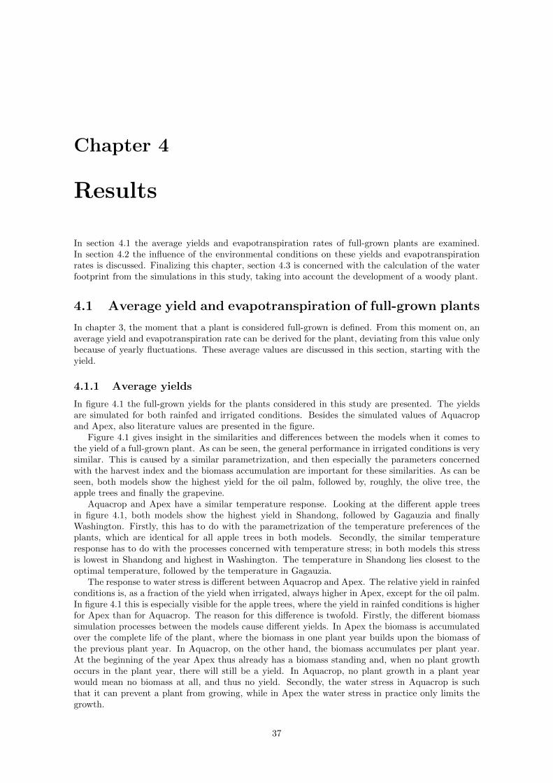
Chapter 4

Results

In section 4.1 the average yields and evapotranspiration rates of full-grown plants are examined.In section 4.2 the influence of the environmental conditions on these yields and evapotranspirationrates is discussed. Finalizing this chapter, section 4.3 is concerned with the calculation of the waterfootprint from the simulations in this study, taking into account the development of a woody plant.

4.1 Average yield and evapotranspiration of full-grown plants

In chapter 3, the moment that a plant is considered full-grown is defined. From this moment on, anaverage yield and evapotranspiration rate can be derived for the plant, deviating from this value onlybecause of yearly fluctuations. These average values are discussed in this section, starting with theyield.

4.1.1 Average yields

In figure 4.1 the full-grown yields for the plants considered in this study are presented. The yieldsare simulated for both rainfed and irrigated conditions. Besides the simulated values of Aquacropand Apex, also literature values are presented in the figure.

Figure 4.1 gives insight in the similarities and differences between the models when it comes tothe yield of a full-grown plant. As can be seen, the general performance in irrigated conditions is verysimilar. This is caused by a similar parametrization, and then especially the parameters concernedwith the harvest index and the biomass accumulation are important for these similarities. As can beseen, both models show the highest yield for the oil palm, followed by, roughly, the olive tree, theapple trees and finally the grapevine.

Aquacrop and Apex have a similar temperature response. Looking at the different apple treesin figure 4.1, both models show the highest yield in Shandong, followed by Gagauzia and finallyWashington. Firstly, this has to do with the parametrization of the temperature preferences of theplants, which are identical for all apple trees in both models. Secondly, the similar temperatureresponse has to do with the processes concerned with temperature stress; in both models this stressis lowest in Shandong and highest in Washington. The temperature in Shandong lies closest to theoptimal temperature, followed by the temperature in Gagauzia.

The response to water stress is different between Aquacrop and Apex. The relative yield in rainfedconditions is, as a fraction of the yield when irrigated, always higher in Apex, except for the oil palm.In figure 4.1 this is especially visible for the apple trees, where the yield in rainfed conditions is higherfor Apex than for Aquacrop. The reason for this difference is twofold. Firstly, the different biomasssimulation processes between the models cause different yields. In Apex the biomass is accumulatedover the complete life of the plant, where the biomass in one plant year builds upon the biomass ofthe previous plant year. In Aquacrop, on the other hand, the biomass accumulates per plant year.At the beginning of the year Apex thus already has a biomass standing and, when no plant growthoccurs in the plant year, there will still be a yield. In Aquacrop, no plant growth in a plant yearwould mean no biomass at all, and thus no yield. Secondly, the water stress in Aquacrop is suchthat it can prevent a plant from growing, while in Apex the water stress in practice only limits thegrowth.

37

From figure 4.1 it can be seen that in irrigated conditions Aquacrop simulates a higher yield thanApex for the apple trees, while it is the other way around for the olive tree and the oil palm. Thishas partly to do with the parametrization of the plant, and more specifically the parametrizationof the biomass. Parameters in Apex and Aquacrop that are not derived from each other in theharmonization procedure are responsible for this. These parameters cause a relative high biomass inAquacrop and a low biomass in Apex for the apple trees, while for the olive tree and the oil palm thisis the other way around. As a result, the yield shows the same pattern. Furthermore, the processesunderlying the biomass accumulation are very different, as Aquacrop simulates biomass as a functionof the transpiration while in Apex it is mainly the solar radiation that is responsible for the biomassaccumulation.

Looking at the average yield of the grapevine in irrigated conditions, it can be seen that theabsolute difference between the models is small. However, the relative difference between the predictedyields is largest of all plants, with Aquacrop yield being eight times higher than the one of Apex. Thecause of this lies purely in Apex and is a combination of a different parametrization compared to theother plants and different processes resulting from this. In Apex, the grapevine is not simulated asa tree like the other plants, but as a shrub. While this seems reasonable, as the grapevine is indeeda shrub, the biomass accumulation for a shrub in Apex is on a yearly basis. This in contrast with alifelong accumulation for trees. This causes a relative low biomass in Apex. Furthermore, the harvestindex in Apex is much lower than the potential one, because of a different simulation of the heatunit index for a shrub as for a tree. The combination of the two cause a lower yield in Apex, butthe first one also results in a deviating yield for Aquacrop; the factor that converts the harvest indexof Apex to the harvest index of Aquacrop is based on trees only and presumes a lifelong biomassaccumulation in Apex. The fact that the grapevine is simulated without this lifelong accumulationmakes the harvest index in Aquacrop relatively high. Note that the yield of the grapevine in rainfedconditions is practically zero in both models, as the water stress is so severe that the plant hardlygrows.

When we look at the yield values of the models in relation to the literature values, it can beseen that the literature values are in general lower than the simulated values. This has multiplecauses. Firstly, the models simulate no fertility stress, diseases or plagues, which in reality do occur.Secondly, the models simulate dry yield while literature values are normally presented as fresh yield.To translate the fresh yield to dry yield the simple relation of Raes et al. (2012) is used, which statesthat the dry weight is approximately a quarter of fresh weight. In reality this depends on the water

Appletree (Sh)

(1994-2010)

Appletree (Ga)

(1994-2010)

Appletree (Wa)

(1995-2010)

Grape-vine

(1981-2010)

Olivetree

(2001-2010)

Oilpalm

(1998-2009)

0

5

10

15

20

25

30

9.78.2

6.1

0.8

8.5

20.3

4.8

0.90.0 0.4

Yield

[ton

/ha/y

ear]

Appletree (Sh)

(1994-2010)

Appletree (Ga)

(1994-2010)

Appletree (Wa)

(1995-2010)

Grape-vine

(1981-2010)

Olivetree

(2001-2010)

Oilpalm

(1998-2009)

0

5

10

15

20

25

30

Yield

[ton

/ha/y

ear]

Malaysia*

33.1 · 106haAndalusia

8.7 · 106haC.La Mancha

7.9 · 106haWashington

18.5 · 106haMoldova*

3.4 · 106haShandong

15.7 · 106ha

Appletree (Sh)

(1994-2010)

Appletree (Ga)

(1994-2010)

Appletree (Wa)

(1995-2010)

Grape-vine

(1981-2010)

Olivetree

(2001-2010)

Oilpalm

(1998-2009)

0

5

10

15

20

25

30

6.85.9

3.8

0.1

12.5

23.1

2.6

0.6

4.5

19.3

Yield

[ton

/ha/y

ear]

Aquacrop rainfed Irrigated Literature Apex rainfed Irrigated

Figure 4.1: The average full-grown yields for the plants considered in this study. The x-axis showsthe plant and the years in the simulation that the plant is considered full-grown. The literature valuesare as location specific as possible; the grey text boxes above the values show the region on whichthey are specified. Locations with an asterisk (*) are on a country level, the rest is on a provincelevel.

38

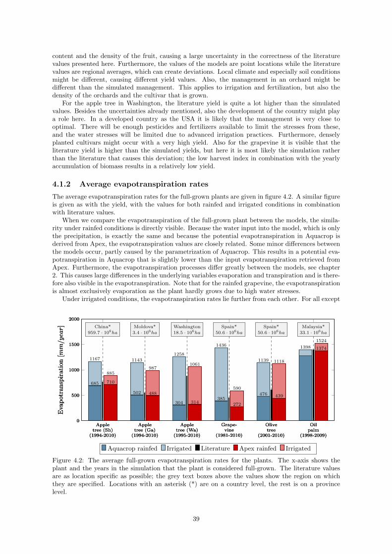
content and the density of the fruit, causing a large uncertainty in the correctness of the literaturevalues presented here. Furthermore, the values of the models are point locations while the literaturevalues are regional averages, which can create deviations. Local climate and especially soil conditionsmight be different, causing different yield values. Also, the management in an orchard might bedifferent than the simulated management. This applies to irrigation and fertilization, but also thedensity of the orchards and the cultivar that is grown.

For the apple tree in Washington, the literature yield is quite a lot higher than the simulatedvalues. Besides the uncertainties already mentioned, also the development of the country might playa role here. In a developed country as the USA it is likely that the management is very close tooptimal. There will be enough pesticides and fertilizers available to limit the stresses from these,and the water stresses will be limited due to advanced irrigation practices. Furthermore, denselyplanted cultivars might occur with a very high yield. Also for the grapevine it is visible that theliterature yield is higher than the simulated yields, but here it is most likely the simulation ratherthan the literature that causes this deviation; the low harvest index in combination with the yearlyaccumulation of biomass results in a relatively low yield.

4.1.2 Average evapotranspiration rates

The average evapotranspiration rates for the full-grown plants are given in figure 4.2. A similar figureis given as with the yield, with the values for both rainfed and irrigated conditions in combinationwith literature values.

When we compare the evapotranspiration of the full-grown plant between the models, the simila-rity under rainfed conditions is directly visible. Because the water input into the model, which is onlythe precipitation, is exactly the same and because the potential evapotranspiration in Aquacrop isderived from Apex, the evapotranspiration values are closely related. Some minor differences betweenthe models occur, partly caused by the parametrization of Aquacrop. This results in a potential eva-potranspiration in Aquacrop that is slightly lower than the input evapotranspiration retrieved fromApex. Furthermore, the evapotranspiration processes differ greatly between the models, see chapter2. This causes large differences in the underlying variables evaporation and transpiration and is there-fore also visible in the evapotranspiration. Note that for the rainfed grapevine, the evapotranspirationis almost exclusively evaporation as the plant hardly grows due to high water stresses.

Under irrigated conditions, the evapotranspiration rates lie further from each other. For all except

Appletree (Sh)

(1994-2010)

Appletree (Ga)

(1994-2010)

Appletree (Wa)

(1995-2010)

Grape-vine

(1981-2010)

Olivetree

(2001-2010)

Oilpalm

(1998-2009)

0

500

1000

1500

2000

1167 1143

1258

1436

1139

1398

685

502

304385

476

Evapotranspiration[m

m/y

ear]

Appletree (Sh)

(1994-2010)

Appletree (Ga)

(1994-2010)

Appletree (Wa)

(1995-2010)

Grape-vine

(1981-2010)

Olivetree

(2001-2010)

Oilpalm

(1998-2009)

0

500

1000

1500

2000


m/y

ear] Malaysia*

33.1 · 106haSpain*

50.6 · 106haSpain*

50.6 · 106haWashington

18.5 · 106haMoldova*

3.4 · 106haChina*

959.7 · 106ha

Appletree (Sh)

(1994-2010)

Appletree (Ga)

(1994-2010)

Appletree (Wa)

(1995-2010)

Grape-vine

(1981-2010)

Olivetree

(2001-2010)

Oilpalm

(1998-2009)

0

500

1000

1500

2000

885987

1061

590

1118

1524

710

488

314 272

439

1374


m/y

ear]


Figure 4.2: The average full-grown evapotranspiration rates for the plants. The x-axis shows theplant and the years in the simulation that the plant is considered full-grown. The literature valuesare as location specific as possible; the grey text boxes above the values show the region on whichthey are specified. Locations with an asterisk (*) are on a country level, the rest is on a provincelevel.

39

the oil palm, the evapotranspiration is higher in Aquacrop. The differences between the models haveto do with two processes. Firstly, the irrigation rigger differs between the models. In both models,irrigation water is applied to prevent water stresses in the plant. In Aquacrop, this irrigation istriggered at a certain depletion of the soil, which in practice results in an evapotranspiration thatis about equal to the potential one. In Apex irrigation is triggered when water stress in the plantoccurs, which results in a transpiration, thus not the whole evapotranspiration, that is about equalto the potential one. Secondly, the irrigation water in Aquacrop becomes available for both theevaporation and the transpiration. In Apex something else happens; when irrigation is applied, theevaporation is hardly affected. This is probably caused by the fact that evaporation in Apex consistsof soil evaporation, litter evaporation (intercepted rainfall) and snow evaporation. While the modeloutput gives only the total evaporation, it seems that the irrigation water only contributes to the soilevaporation, leaving the other two components untouched. Evaporation from litter and snow form amajor part of the total evaporation, causing the total evaporation to be hardly affected by irrigationwater. The irrigation thus almost exclusively contributes to transpiration alone.

Comparing the evapotranspiration rates from the models with literature vales, it becomes visiblethat there is a lot of resemblance. The literature values lie between irrigated and rainfed evapotrans-piration. This makes sense, as a region will probably have both irrigated and rainfed orchards of acertain plant. The arguments for the literature values of the yield also apply here, and deviationsfrom literature can thus occur because of different management practices and differences in location.

4.1.3 Concluding

In the previous two sections, the average yields and evapotranspiration rates of full-grown plantswere presented, together with an explanation for the differences and similarities between the models.These explanations could all be traced back to either the parametrization of the plant, the underlyingsimulation processes in the models or the input into the models. Table 4.1 summarizes the similaritiesand differences, including their causes.

Table 4.1: An overview of the similarities and differences in the simulation of full-grown yields andevapotranspiration rates. The causes can be traced back to parametrization of the models, theprocesses in the models or the input.

Similarity or difference CauseThe models show a very similar yield pattern between plants ParametrizationAquacrop and Apex show a similar response on temperature Parametrization, processesAquacrop responds stronger on water stress than Apex ProcessesSometimes highest yield for Aquacrop, other times for Apex Parametrization, processesApex shows a very low yield for the grapevine Parametrization, processesLarge differences occur with the literature yieldAquacrop and Apex show almost the same rainfed evapotr. InputLarge differences can occur in irrigated evapotranspiration ProcessesMuch similarity with the literature evapotranspiration

4.2 Environmental effects on the full-grown yield and evapo-transpiration

Because of climate fluctuations over the plant years, deviations occur from the average full-grownyields and evapotranspiration rates presented in section 4.1. In the first section, this variabilityof the yield and evapotranspiration is discussed. In the second section, the influence of the otherenvironmental aspect, the soil profile, is discussed.

4.2.1 Climatic variability

To analyse the climate variability, the yield and evapotranspiration are discussed separately. For thiswe will look at the average values per plant year, still for the full-grown years alone.

40

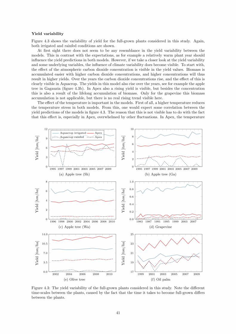
Yield variability

Figure 4.3 shows the variability of yield for the full-grown plants considered in this study. Again,both irrigated and rainfed conditions are shown.

At first sight there does not seem to be any resemblance in the yield variability between themodels. This in contrast with the expectations, as for example a relatively warm plant year shouldinfluence the yield predictions in both models. However, if we take a closer look at the yield variabilityand some underlying variables, the influence of climate variability does become visible. To start with,the effect of the atmospheric carbon dioxide concentration is visible in the yield values. Biomass isaccumulated easier with higher carbon dioxide concentrations, and higher concentrations will thusresult in higher yields. Over the years the carbon dioxide concentrations rise, and the effect of this isclearly visible in Aquacrop. The yields in this model also rise over the years, see for example the appletree in Gagauzia (figure 4.3b). In Apex also a rising yield is visible, but besides the concentrationthis is also a result of the lifelong accumulation of biomass. Only for the grapevine this biomassaccumulation is not applicable, but there is no real rising trend visible here.

The effect of the temperature is important in the models. First of all, a higher temperature reducesthe temperature stress in both models. From this, one would expect some correlation between theyield predictions of the models in figure 4.3. The reason that this is not visible has to do with the factthat this effect is, especially in Apex, overwhelmed by other fluctuations. In Apex, the temperature

1995 1997 1999 2001 2003 2005 2007 20090

3

6

9

12

Yie

ld[ton/ha]

Aquacrop irrigated Apex

Aquacrop rainfed Apex

(a) Apple tree (Sh)

1995 1997 1999 2001 2003 2005 2007 20090

2

4

6

8

10

Yie

ld[ton/ha]

(b) Apple tree (Ga)

1996 1998 2000 2002 2004 2006 2008 20100

2

4

6

8

Yie

ld[ton/ha]

(c) Apple tree (Wa)

1983 1987 1991 1995 1999 2003 20070.0

0.2

0.4

0.6

0.8

1.0

Yie

ld[ton/ha]

(d) Grapevine

2002 2004 2006 2008 20100.0

3.5

7.0

10.5

14.0

Yie

ld[ton/ha]

(e) Olive tree

1999 2001 2003 2005 2007 200917

19

21

23

25

Yie

ld[ton/ha]

(f) Oil palm

Figure 4.3: The yield variability of the full-grown plants considered in this study. Note the differenttime-scales between the plants, caused by the fact that the time it takes to become full-grown differsbetween the plants.

41

affects the accumulation of heat units, and for reasons not mentioned in the documentation, the heatunit index declines when reaching a certain value or at certain events (harvest). As a result, the heatunit index at harvest can fluctuate over the years, and with this the harvest index and thus the yield.It is especially this undocumented process that is visible in the yield variability of Apex, which is bestnoticeable for the oil palm in figure 4.3f. The heat unit index at harvest shows a stepwise pattern,and the exact same thing is visible in the yield, both for the irrigated case and the rainfed case.

In Aquacrop the temperature affects the yield in another way. As harvest occurs at a certainamount of accumulated heat units after green-up, a warmer year would result in an early harvest. Asa result of this, the next plant year starts earlier, as this starts right after harvest to keep the canopycover intact through the winters (see chapter 3). This causes the next plant year to be longer andbecause of this, this plant year will have a higher biomass and thus a higher yield in Aquacrop.

The effect of a fluctuating precipitation pattern is visible for Aquacrop. In rainfed conditions,lower precipitation in a plant year will not directly result in a lower yield, but a lack of precipitation atthe right time will. It is thus not the amount of precipitation that is important, but rather the timingand distribution over the year. This will influence the soil-moisture content in the soil-water balanceand can create water stress at moments that a plant cannot have much. This is for example visiblefor the apple tree in Gagauzia (figure 4.3b), where many years are characterized by zero biomass andthus zero yield. This is caused by a too low soil-moisture content at the very beginning of the plantyear, from which the plant dies right away. If the green-up date would have been later in the year,the plant might still have grown. Furthermore, also the soil-water content during the plant year isrelevant, which is for example visible for the apple tree in Shandong (figure 4.3a). The year 2006 isone of the driest years for the full-grown tree. However, as the lack of precipitation occurs mainlyin the winter, the soil-moisture content is high enough in the summer to limit the amount of waterstress. This in contrast with 1997, which is also a dry year but is characterized by a low summerprecipitation and soil-moisture content. As a result, there is hardly any plant growth taking placeand a near zero yield marks this year. The precipitation of course also affected the water stress inApex. However, the lifelong biomass accumulation limits the influence within a plant year. Also thedominant effect of the heat unit index on the yield causes the yearly effect of precipitation to remainunseen.

In Apex, there is also the effect of a fluctuating solar radiation. However, for the same reasons aswith the carbon dioxide concentration and the precipitation, the effect of this is invisible. A slightcorrelation between the solar radiation and the biomass accumulation is only visible for the grapevine.

Evapotranspiration variability

In figure 4.4 the variability of the evapotranspiration is visible. In contrast with the yield variability,both models show a very similar trend in the evapotranspiration rates over the years. In rainfedconditions the evapotranspiration rates lie closer together as in irrigated conditions, because of thefact that the irrigation trigger and the irrigation amounts differ.

When we look at the effect of the climate variables on the evapotranspiration variability, thereare two variables that cause the resemblance in evapotranspiration variability visible in figure 4.4.Firstly, the temperature has a major effect on the evapotranspiration. In the models, this effecthas two sides. The direct effect is that a warm plant year will have a high evapotranspiration rate,because of the positive relation between temperature and evapotranspiration. The indirect effect isthat a high temperature will shorten the plant year, because of the use of heat units. This causes arelative large fraction of the plant year to fall in the summer months, where the evapotranspiration ishighest. This increases the average evapotranspiration. In irrigated conditions, it is the temperaturethat causes the variability we see at the plants.

The second variable that influences the evapotranspiration is the precipitation. For the irrigatedplants, the precipitation is only important for the distribution of evaporation and transpiration inApex, as intercepted rain by the leaves causes the evaporation to go up and the transpiration to godown. For the rainfed case it is much more important, as the evapotranspiration that can take placedepends on the water availability. More available water will result in a higher evapotranspiration.However, a change of precipitation will not directly cause a similar change in evapotranspiration.Just as with the yield, also the timing and distribution of the rainfall is important. Precipitation inwinter will only have a limited effect on the evapotranspiration, as the potential evapotranspiration islimited because of the temperature. At the same time, intense rainfall events cause overland runoff,

42

1995 1997 1999 2001 2003 2005 2007 2009500

700

900

1100

1300Evapotr.[m

m]

Aquacrop irrigated Apex

Aquacrop rainfed Apex

(a) Apple tree (Sh)

1995 1997 1999 2001 2003 2005 2007 2009300

500

700

900

1100

1300

Evapotr.[m

m]

(b) Apple tree (Ga)

1996 1998 2000 2002 2004 2006 2008 2010200

500

800

1100

1400

Evapotr.[m

m]

(c) Apple tree (Wa)

1983 1987 1991 1995 1999 2003 2007200

600

1000

1400

1800

2200

Evapotr.[m

m]

(d) Grapevine

2002 2004 2006 2008 2010300

500

700

900

1100

1300

Evapotr.[m

m]

(e) Olive tree

1999 2001 2003 2005 2007 20091100

1200

1300

1400

1500

1600

Evapotr.[m

m]

(f) Oil palm

Figure 4.4: The variability of the evapotranspiration rate for the full-grown plants considered in thisstudy. Just as with the yield variability, also here the time-scales differ between the subfigures.

without affecting the evapotranspiration much. In the rainfed cases in figure 4.4, it is the combinedinfluence of the temperature and the precipitation that influences the evapotranspiration rates.

Although solar radiation also influences the potential evapotranspiration rate in Apex and thusthe reference evapotranspiration in Aquacrop, the evapotranspiration function used in this study, theHargreaves function, uses the clear day radiation, without considering the cloud cover. As this isonly a function of the day of the year and the latitude, this will not change over the years and is thusirrelevant for the evapotranspiration variability.

4.2.2 Influence of soils

The influence of the soil profile on the simulated yields and evapotranspiration rates is relevant forrainfed conditions only, although minor differences can occur in irrigated conditions as well. Theinfluences of different soil profiles as a percentage of the original yield and evapotranspiration is givenin table 4.2.

Looking at the table, the first thing that can be noticed is that Aquacrop responds more stronglyto a changing soil profile than Apex, especially for the yield. This is caused by the water stress ina similar way as the climatic variability affected the yield. In Aquacrop a small change in soil-watercontent can have large consequences for the yield. The water stress consists of many components,and in each of these components the change can cause the water content to be just above or below theminimum threshold required for yield forming. In Apex the influence of the soil profile on the yield is

43

Table 4.2: The influence of the different soils on the yield and evapotranspiration in Shandong underrainfed conditions for the full-grown plants only. The percentage of yield and evapotranspirationwith regard to the original soil is shown. The soil number refers to the topsoil/subsoil combinationas given by De Lannoy et al. (2014).

Yield EvapotranspirationSoil layer Aquacrop Apex Aquacrop Apex224/55 (original) 100.0 100.0 100.0 100.08/8 86.2 100.9 101.3 100.5234/234 88.3 89.9 88.3 91.282/172 84.4 98.9 97.8 99.0

limited, because (a) the water stress reduces gradually and is not characterized by these thresholds,because (b) Apex uses a minimum stress factor composed of also temperature stress and aerationstress and water stress is the limiting factor only in less than half of the simulation days, and because(c) the stress only limits the growth of a plant and does not stop it. With a changing plant also thetranspiration is affected, but because this is compensated by a change of evaporation, the change ofevapotranspiration is limited.

The second thing that can be noticed is that soil type 8/8 shows an increase of yield and evapo-transpiration compared to the original soil for Apex. In Aquacrop, however, the evapotranspirationincreases while the yield decreases. Looking at this soil profile we see an increase of both field capacityand wilting point in relation to the original profile, but the field capacity rises more than the wiltingpoint. As a result, the distance between field capacity and wilting point increases. To keep the watercontent at the same point between field capacity and wilting point, more water is required. This waterrequirement for the evapotranspiration and thus the yield is determined by the infiltration (input)and the drainage (output). In Aquacrop this amount of water cannot be provided as the infiltration islow. In this model, infiltration is determined by both the curve number and the saturated hydraulicconductivity of this soil profile. In Apex the infiltration is only determined by the curve number andis therefore relatively high. For this reason the relative water content in Aquacrop decreases whilethe relative water content in Apex increases. As a result, a similar pattern is visible in the yield.The evapotranspiration in Aquacrop rises because the decrease in transpiration is compensated by alarger increase of evaporation.

4.2.3 Concluding

In section 4.2 the variability of the yields and evapotranspiration rates as a result of the fluctuatingclimate has been discussed. Also the effect the soil conditions have on the models is explained. Intable 4.3 the effects of the climate and soil conditions are summarized.

Table 4.3: An overview of the effect of the climate conditions and soil conditions on the yields andevapotranspiration rates in Aquacrop and Apex.

Environmental condition Effect on modelsCarbon dioxide conc. Affects yield, but in Apex overwhelmed by heat unit indexPrecipitation Can affect yield and evapotranspiration when rainfedTemperature Affects yield and evapotranspirationSolar radiation Affects yield in Apex, but overwhelmed by heat unit indexSoil profile Affects Aquacrop more than Apex when rainfed

4.3 The influence of plant development and the water foot-print

Before a plant reaches its full-grown yield and evapotranspiration rate, it experiences a period in whichthe yield and evapotranspiration develops. This development, and more specifically, the importanceof this development in the calculation of the water footprint, is examined here.

44

1983 1987 1991 1995 1999 2003 20070

2

4

6

8Y

ield

[ton/ha]

Lifelong development

Full-grown years

Average full-grown value

(a) Yield, apple tree (Sh)

1983 1987 1991 1995 1999 2003 2007700

900

1100

1300

1500

Evapotr.[m

m]

(b) Evapotranspiration, apple tree (Sh)

1983 1987 1991 1995 1999 2003 20070

2

4

6

8

Yie

ld[ton/ha]

(c) Yield, apple tree (Ga)

1983 1987 1991 1995 1999 2003 2007700

900

1100

1300

1500

Evapotr.[m

m]

(d) Evapotranspiration, apple tree (Ga)

1983 1987 1991 1995 1999 2003 20070

1

2

3

4

5

Yie

ld[ton/ha]

(e) Yield, apple tree (Wa)

1983 1987 1991 1995 1999 2003 2007900

1100

1300

1500

Evapotr.[m

m]

(f) Evapotranspiration, apple tree (Wa)

1983 1987 1991 1995 1999 2003 20070

3

6

9

12

15

Yie

ld[ton/ha]

(g) Yield, olive tree

1983 1987 1991 1995 1999 2003 2007900

1100

1300

1500

1700

Evapotr.

[mm]

(h) Evapotranspiration, olive tree

1983 1987 1991 1995 1999 2003 20070

5

10

15

20

25

30

Yie

ld[ton/ha]

(i) Yield, oil palm

1983 1987 1991 1995 1999 2003 20071400

1450

1500

1550

1600

Evapotr.

[mm]

(j) Evapotranspiration, oil palm

Figure 4.5: The Apex simulation of yield and evapotranspiration growth towards the full-grown years.Grapevine is left out of this figure, as this plant is simulated as full-grown the whole period (see figure4.3d). The simulations are all irrigated.

45

In figure 4.5 an overview is given of the development curve found in Apex. During the 30 years ofsimulation in this study, the yield grows towards a certain equilibrium as a result of biomass growththat follows a similar pattern. However, the time it takes for a plant to become full-grown differs. Theapple trees reach their full-grown phase quite fast, while the olive tree is still developing at the end ofthe simulation period. The oil palm lies in between these. The different lengths of the developmentphases are probably caused by a different parametrization, although this cannot be traced back to thedocumentation of Apex. Because of the development phase, the lifelong average yield, which includesthe yield in this development phase, is lower than the yield of a full-grown plant. It is worth noticingthat in reality, in contrast with what Apex shows here, the yield does not continue to increase over aplants life. At some point the productivity of a tree reaches an optimum, where after the yield slowlydecreases (see for example Flore et al. (1984)).

The evapotranspiration also shows development over a plants life. As can be seen in figure 4.5, thefirst few years show a different evapotranspiration rate. In these years, where the leaves still develop,the distribution of evapotranspiration over evaporation and transpiration changes. With the leaf areagrowing, the amount of evaporation decreases while the amount of transpiration increases. As theevaporation declines more than the transpiration inclines, the initial years are characterized by ahigher evapotranspiration. For the oil palm it is the other way around, as the transpiration increasesmore than the evaporation decreases. Because this initial anomaly is short in time and becausethe evapotranspiration is much more variable in general, the lifelong average evapotranspiration ratedeviates only little from the average evapotranspiration rate of the full-grown tree.

Figure 4.6 shows the ratios between the lifelong results and the full-grown results. These factorsshow the importance of the development phase and can be used to adjust the results of a simulationfor the full-grown period only to the lifelong results. As can be seen, the yield has a factor thatis well below one, meaning that the lifelong yield is indeed lower than the full-grown yield. Theevapotranspiration factors for the plants considered in this study only slightly deviate from one.When simulating yields of full-grown plants, the figure shows the relevance of correcting these to thelifelong average results. For the evapotranspiration this is not necessary, as the lifelong results arepractically equal to the full-grown evapotranspiration rates.

Knowing the importance of the development phase on the yield and evapotranspiration, the waterfootprint can be calculated by using this factor to correct the yield of Aquacrop to include thedevelopment phase as well. For the water footprint calculated for Apex no factor is applied, as thelifelong average evapotranspiration and the lifelong average yield can be directly used from the model.In figure 4.7 the water footprints are calculated for all plants considered in this study. Note that thewater footprint calculation requires fresh weight; to convert the dry weight from the models to fresh

Appletree (Sh)

Appletree (Ga)

Appletree (Wa)

Grape-vine

Olivetree

Oilpalm

0.6

0.8

1

1.2

1.4

0.82 0.81 0.80

0.67

0.77

Factor[−

]

Appletree (Sh)

Appletree (Ga)

Appletree (Wa)

Grape-vine

Olivetree

Oilpalm

0.6

0.8

1

1.2

1.4

1.01 1.001.04

1.021.00

Factor[−

]

Yield Evapotranspiration

Figure 4.6: The factors that relate lifelong results with the average values for yield and evapotrans-piration. Note that grapevine is not considered as this plant is simulated in Apex as full-grown thewhole period. The factors are derived for irrigated conditions.

46

Appletree (Sh)

Appletree (Ga)

Appletree (Wa)

Grape-vine

Olivetree

Oilpalm

0

1000

2000

3000

4000

500052857

478

2052

3202

241

Waterfootprint[m

3/ton

]

Appletree (Sh)

Appletree (Ga)

Appletree (Wa)

Grape-vine

Olivetree

Oilpalm

0

1000

2000

3000

4000

5000248885

438679

4388

515

Waterfootprint[m

3/ton

]

Appletree (Sh)

Appletree (Ga)

Appletree (Wa)

Grape-vine

Olivetree

Oilpalm

0

1000

2000

3000

4000

5000Waterfootprint[m

3/ton

]

Appletree (Sh)

Appletree (Ga)

Appletree (Wa)

Grape-vine

Olivetree

Oilpalm

0

1000

2000

3000

4000

5000

401595

1586

366228

Waterfootprint[m

3/ton

]

Appletree (Sh)

Appletree (Ga)

Appletree (Wa)

Grape-vine

Olivetree

Oilpalm

0

1000

2000

3000

4000

500013605

899

Waterfootprint[m

3/ton

]


Figure 4.7: The water footprints of the plants considered in this study, both in rainfed and irrigatedconditions. For Aquacrop, the factor from figure 4.6 is used to get lifelong yield, the grapevine has afactor 1. For Apex, no factor is applied. The literature values are on a province level, except for theapple tree in Moldova. The literature values are retrieved from Mekonnen and Hoekstra (2010).

weight, all yields are multiplied by a factor four (Raes et al., 2012).As can be seen in the figure, the rainfed water footprint is almost always higher than the irrigated

water footprint. This might seem unnatural, but as the yield can be much lower in rainfed conditionsthan in irrigated conditions, the water footprint can be much higher. One might wonder the usefulnessof the rainfed water footprint in this case, as the high water stress can result in very low yields. Theresulting water footprint can be very large or even infinite. For the grapevine, it can be seen that thewater footprint is also very large in irrigated conditions, caused by the low yield of the plant. Thisraises questions about the correct implementation of the grapevine in the models.

In general, the performance of the models is quite alike for irrigated conditions, but can differtremendously in rainfed conditions because of the differences in yields between the models. Thedifference with literature can be large, caused by the deviation between the simulated yield and theliterature yield that lies at the foundations of the water footprint calculations.

47

Chapter 5

Discussion

The methods and the models are discussed in the coming sections. First, the performance of woodiesin Aquacrop and Apex is discussed, where after the difference between this study and literature isdiscussed when simulating a woody plant in Aquacrop. Finally, the applicability of this study forother studies is described.

5.1 The performance of woodies in Aquacrop and Apex

The results of Aquacrop and Apex can differ quite a lot. When rainfed, the evapotranspiration isquite alike but the yield can differ tremendously because of the difference between the models insimulating water stress. When irrigated, the evapotranspiration rates lie often far from each otherbecause of a different simulation of irrigation water.

These different results are striking, but unfortunately there is no such thing as a reference thatstate the correct value and help us decide which model is ’good’ and which model is ’bad’. Thedifference does not have to be a flaw of the implementation of woodies in Aquacrop and can bejust as easy be a problem in Apex. It is exactly this uncertainty that makes it hard to draw solidconclusions from the results. What does help is the further analysis that identifies some ordinarybehaviour in especially Apex. The yield in this model is mainly driven by the variable heat unitindex, which can show for a full-grown tree very conspicuous behaviour. Also the distribution ofirrigation water to almost exclusively the transpiration is something that is questionable for Apex.On the other hand, the sensitivity of Aquacrop for the soil water content, where a small differencecan lead to large changes in the biomass and the yield, might be realistic for herbaceous plants. Forwoody plants the stress effects are however more limited (Steduto et al., 2012).

Thus both models seem to have limitations, but on top of that there is also uncertainty in theparametrization in both models. In Aquacrop, one of the main consequences of only simulating thefoliage is the adjustment of the harvest index. However, in this study this is taken very roughlyas a factor four of the normal harvest index, as the weight of the total biomass is approximately afactor four of the foliage. But of course this can differ tremendously between plants. Furthermore, thecanopy cover in Aquacrop is derived from the leaf area index of Apex in order to harmonize the models,but the relation used is based on herbaceous plants and its applicability on woodies is rather uncertain.If the parameter assumptions prove to be incorrect, a very different yield and evapotranspiration mightbe the result. At the same time also Apex has problems in the parametrization, which become visiblefor especially the grapevine. This plant is simulated as a shrub rather than a tree, resulting in ayearly, instead of lifelong, accumulation of biomass as if it is a herbaceous plant, which seems veryunrealistic. Also the parametrization of trees is doubtful, as plants as the oil palm or the olive tree,which are evergreen plants according to literature, are parametrised as deciduous plants in Apex.

In short, there are large uncertainties in both models. The method to simulate woodies inAquacrop does not seem to be inferior to the simulations of woodies in Apex.

48

5.2 Comparison of Aquacrop simulation with literature

The implementation of woody plants in Aquacrop is rather different as the studies so far, althoughthe number of studies that simulate woody plants with Aquacrop is limited. Hunink and Droogers(2010) and Hunink and Droogers (2011) estimated the parameters regarding the planting date, theharvest date, the harvest index, the canopy cover and the management based on reasoning andliterature. Zhuo et al. (2016) set the properties planting date, harvest index, rooting depth and thelength of different growth stages based on literature. All of these studies do not discriminate betweenherbaceous plants and woody plants; only the parameter values differ between the plants.

This study proposes an alternative method to simulate woodies. Of course, a number of parametersshould be selected for the different plants, in this study mainly based on the parameters of Apex forharmonization between the models. However, by keeping the canopy cover intact through the winter,by increasing the harvest index to account for the foliage weight only and by choosing a constantrooting depth corresponding to that of a full-grown woody, a few fundamental differences in parametersettings and model use occur between the studies so far and the simulation of woodies in this study.

The relevant question is, of course, if this different approach leads to truly different yield, eva-potranspiration and resulting water footprint values. Fortunately Zhuo et al. (2016) made theirAquacrop plant file for the apple tree available for this study. They used the method described byHoekstra et al. (2011) to calculate the water footprint, which would mean that for perennial plants, asthe apple tree is, the yield and evapotranspiration is averaged over the complete life of the plant forthe calculation of the water footprint. So this is the evapotranspiration rate from the first plantingdate up to the last harvest date, although during the time between harvest in one season and plantingin the following season no plant grows. For the yields these are just the average yields at harvest.

When using the original plant file of Zhuo et al. (2016), which was used for the Yellow RiverBasin in China, for the Shandong point simulation of in this study under irrigated conditions, anaverage lifelong yield for the period 1981 to 2010 of 3.4 ton/ha is retrieved, against 9.3 ton/ha inthis study. The evapotranspiration for Zhuo et al. (2016) is 1017 mm/year, against 1165 mm/yearin this study. Especially the difference in yield is very large, which would have a great effect on thewater footprint.So the method proposed here leads to very different results than the method used byZhuo et al. (2016). Note that the original file of Zhuo et al. (2016) is used here, without any changes.This results in, among others, a different growing method (in days instead of heat units), a differentrooting depth, a different harvest index, a different canopy development and different temperaturepreferences. This explains the large difference in yield and evapotranspiration.

Because of the differences in parametrization, large deviations in the resulting yield and evapo-transpiration are not surprising. To analyse only the effect of the rooting depth and winter canopyon woodies, another simulation of Aquacrop is done. The plant file used in this study is simulatedagain, but now without the constant rooting depth and without the winter canopy. This again underirrigated conditions. With this, a yield is found of 8.5 ton/ha instead of the 9.3 ton/ha in the originalsimulation. The evapotranspiration is now 981 mm/year. As can be seen, the difference in yield issmaller, but the difference in evapotranspiration increases. The woody set-up, without changing therest of the parameters, thus leads to different yields and evapotranspiration values.

5.3 Applicability of methods and results

In this study only four plants are tested on a field level. To draw solid conclusions of the performanceof Aquacrop and Apex, a wider analysis is required. Ideally, a comparison to measured yields andevapotranspiration rates is made for an orchard from which the management and plant conditionsare known. The local plant density, the canopy cover and leaf area index, but also the weight of thefoliage in comparison to the whole aboveground biomass are properties that are assumed in this studywithout much certainty. When these properties can be measured, a better estimate of the parametersfor the trees and shrubs can be made. With this, a very good comparison between simulated yieldand evapotranspiration and measured yield and evapotranspiration can be made. It would then alsobe unnecessary to derive parameters from Aquacrop from Apex and the other way around. Insteadof setting up the models such that Aquacrop and Apex are as much alike as possible, the models willboth be set-up to simulate the considered orchard as good as possible.

More plants should be simulated in combination with a grid-based study to make a more com-

49

prehensive comparison between the models. More climate and soil conditions can be simulated, andthe performance of the models for a wider range of plants can be analysed. Also a better comparisonwith literature is then possible, as these values are mostly available on a country or province scale.

With an expansion of this study to make a more comprehensive comparison with literature and todraw more solid conclusions on the simulated yields and evapotranspiration rates, more confidence ofthe performance of the two models is gained. This study forms the basis for such a more comprehensivestudy. Future studies benefit from this as they can make a more reliable simulation of woodies.

50

Chapter 6

Conclusions & recommendations

By selecting four important woody plants, the apple tree, the grapevine, the olive tree and the oilpalm, and simulating them on the locations in the world where they are cultivated most, Aquacrop andApex are compared in their simulated yields and evapotranspiration rates under different climatic andsoil conditions. To simulate woodies with Aquacrop, for which the model is not designed, Aquacrophas been set-up to simulate only the annual foliage development of a full-grown tree. The model set-up and parametrization of Aquacrop and Apex are harmonized in order to make a fair comparisonpossible.

6.1 Conclusions

For full-grown woody plants, Aquacrop and Apex show roughly the same yield and evapotranspi-ration patterns over the different plants. Both Aquacrop and Apex show in irrigated conditionsthe highest yield for the oil palm and the lowest yield for the grapevine. In rainfed conditions, theevapotranspiration rates between the models are closely related. When we look at specific plants,however, large differences can be observed between the models, caused by differences in the input, theparametrization and the simulation of processes. The response of the models to different temperatureregimes is comparable, but the influence of water stress in the models is very different. In Aquacropthe simulated yield can be reduced a lot from only a small increase of water stress, while Apex is stillable to produce a rather high yield even under severe water stress. When we look at the evapotrans-piration, it is observed that the irrigation water contributes to both evaporation and transpirationin Aquacrop, which is realistic for the sprinkler type irrigation used in this study. In Apex, however,irrigation almost exclusively contributes to transpiration alone. When we compare the evapotrans-piration rates with literature values, the literature always lies between the rainfed and the irrigatedevapotranspiration, which makes sense as a country would have both rainfed and irrigated orchards.Compared to literature, the models however overestimate the yields for most plants.

The climatic influence in the models on the evapotranspiration is very similar. An increase intemperature or available water leads in both models to an increase of evapotranspiration, whichis logic behaviour if we look at the evapotranspiration function. Looking at the yield, Aquacropshows fluctuations that correspond to the climatic variability, although the effect of the woody set-upapplied in this study becomes visible. The yield fluctuations in Apex are driven completely by amodel variable that shows very erratic behaviour, not corresponding to any of the climatic variables.In underlying variables in Apex there is correspondence with climatic variables. The influence of thesoil profile on the simulated yields and evapotranspiration rates are quite different, caused by therather strong response of Aquacrop to a changing water stress.

To calculate the water footprint, the lifelong average yields and evapotranspiration rates shouldbe known. This includes the full-grown years, but also the years in the beginning of a plants lifewhere the plant is still developing. The effect of this development phase can be analysed with Apex.For the evapotranspiration this development is negligible. When we look at the yield, however, thedevelopment phase causes a decrease of about 20 percent in the lifelong average yield compared tothe full-grown yield. Knowing this, the water footprints can be calculated for the plants in bothmodels. These water footprints are quite similar between the models in irrigated conditions, but the

51

differences in rainfed conditions can be large. Also the difference with literature values can be large,caused by the yields underlying the water footprint values.

At first sight the performance of the models is rather similar. However, when taking a closer looklarge differences can be observed. The causes of these differences lie in both Aquacrop and Apex.Comparing the results of Aquacrop, Apex and literature, it cannot be stated that one model is betterthan another. But from this study, Aquacrop does not seem to be inferior to Apex when simulatingwoodies, despite the fact that it is not designed for this.

6.2 Recommendations

This study forms the basis for a more comprehensive comparison between Aquacrop and Apex. Fur-ther study should focus on expanding the scope, firstly by including more plants. In this study threebroadleaved trees and a broadleaved shrub were simulated.In addition more trees and especially moreshrubs, both broadleaved and needle-leaved, should be simulated. Secondly, a grid-based simulationof plants should be done in order to make a better comparison to literature. The differences betweenliterature and the simulated values of especially the yield and water footprint are large, but as thesevalues are often available on a province or even a country level, it is difficult to say whether thedifferences are caused by the simulation processes or by the scale differences. A more comprehensivegrid-based study will avoid these scale differences.

Besides the expansion of the scope, a case study is recommended to analyse the performance ofthe models. This will not only allow for a better comparison with external data, but this study canalso be used to find better values for the parameters in the models. Parameters as the harvest index,the canopy cover and the leaf area index are important for the resulting yield and evapotranspiration,but their values are uncertain. The harmonization in this study caused the models to be comparableto each other, but did not result in an optimal setting with respect to literature. With a case studythe important parameters can be estimated independently for Aquacrop and Apex and a bettercomparison between the models and with external data is possible.

52

Bibliography

Adam, M., L. G. J. Van Bussel, P. A. Leffelaar, H. Van Keulen, and F. Ewert (2011), Effects ofmodelling detail on simulated potential crop yields under a wide range of climatic conditions,Ecological Modelling, 222, 131–143.

Alcamo, J., M. Florke, and M. Marker (2007), Future long-term changes in global water resourcesdriven by socio-economic and climatic changes, Hydrological Sciences Journal, 52 (2), 247–275.

Allen, R. G., L. S. Pereira, D. Raes, and M. Smith (1998), Crop evapotranspiration - guidelines forcomputing crop water requirements, no. 56 in Irrigation and drainage paper, FAO, Rome, Italy.

Allen, R. G., L. S. Pereira, D. Raes, and M. Smith (2006), Crop evapotranspiration - guidelines forcomputing crop water requirements, no. 56 in Irrigation and drainage paper, FAO, Rome, Italy.

Balkovic, J., M. Van der Velde, E. Schmid, R. Skalsky, N. Khabarov, M. Obersteiner, B. Sturmer,and W. Xiong (2013), Pan-European crop modelling with Epic: implementation, up-scaling andregional crop yield validation, Agricultural Systems, 120, 61–75.

Beers, E. H., and L. A. Hull (1995), Dry matter partitioning of nonbearing apple trees followinginjury by European red mite, Journal of Economic Entomology, 88 (4), 998–1003.

Brisson, N., et al. (2003), An overview of the crop model stics, European Journal of Agronomy, 18,309–332.

Chapagain, A. K., and A. Y. Hoekstra (2004), Water footprints of nations, no. 16 in Value of WaterReserach Report Series, Unesco-IHE, Delft, The Netherlands.

Corley, R. H. V., and P. B. Tinker (2016), The Oil Palm, 5th ed., Wiley.

De Graaf, I. E. M., L. P. H. Van Beek, Y. Wada, and M. F. P. Bierkens (2014), Dynamic attributionof global water demand to surface water and ground water resources: effects of abstractions andreturn flows on river discharges, Advances in Water Resources, 64, 21–33.

De Lannoy, G. J. M., R. D. Koster, R. H. Reichle, S. P. P. Mahanama, and Q. Liu (2014), Anupdated treatment of soil texture and associated hydraulic properties in a global land modelingsystem, Journal of Advances in Modeling Earth Systems, 6, 957–979.

Dee, D. P., et al. (2011), The era-interim reanalysis: configuration and performance of the dataassimilation system, Quarterly Journal of the Royal Meteorological Society, 137, 553–597.

Doll, P., and S. Siebert (2002), Global modeling of irrigation water requirements, Water ResourcesResearch, 38 (4), 8.1–8.10.

Faostat (2015), Faostat database, downloaded on 22-12-2015, http://faostat3.fao.org/.

Flore, J. A., G. DeGrandt-Hoffman, and R. L. Perry (1984), Apple tree growth and development, inMonitoring in apple orchards: an instruction manual, Battenfield and Berney.

Galan, C., H. Garcıa-Mozo, L. Vazquez, L. Ruiz, C. Dıaz de la Guardia, and E. Domınquez-Vilches(2008), Modeling olive crop yield in Andalusia, Spain, Agronomy Journal, 100 (1), 98–104.

53

http://faostat3.fao.org/

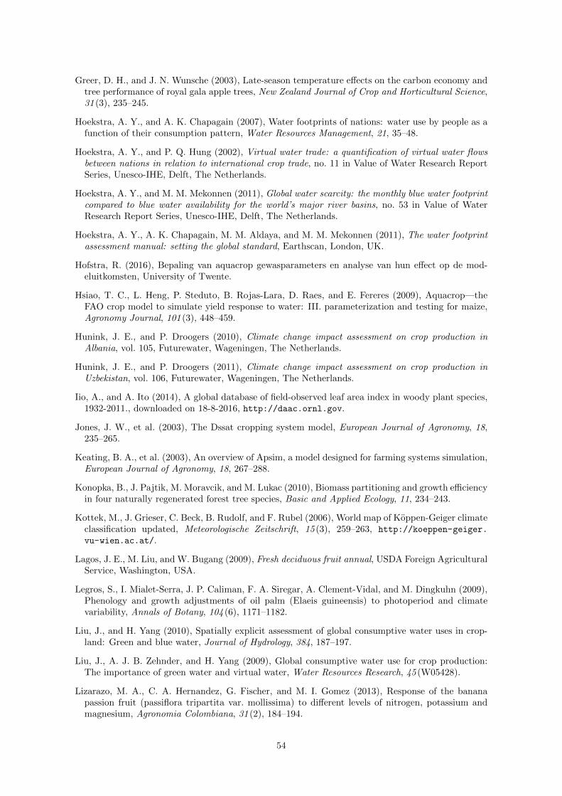
Greer, D. H., and J. N. Wunsche (2003), Late-season temperature effects on the carbon economy andtree performance of royal gala apple trees, New Zealand Journal of Crop and Horticultural Science,31 (3), 235–245.

Hoekstra, A. Y., and A. K. Chapagain (2007), Water footprints of nations: water use by people as afunction of their consumption pattern, Water Resources Management, 21, 35–48.

Hoekstra, A. Y., and P. Q. Hung (2002), Virtual water trade: a quantification of virtual water flowsbetween nations in relation to international crop trade, no. 11 in Value of Water Research ReportSeries, Unesco-IHE, Delft, The Netherlands.

Hoekstra, A. Y., and M. M. Mekonnen (2011), Global water scarcity: the monthly blue water footprintcompared to blue water availability for the world’s major river basins, no. 53 in Value of WaterResearch Report Series, Unesco-IHE, Delft, The Netherlands.

Hoekstra, A. Y., A. K. Chapagain, M. M. Aldaya, and M. M. Mekonnen (2011), The water footprintassessment manual: setting the global standard, Earthscan, London, UK.

Hofstra, R. (2016), Bepaling van aquacrop gewasparameters en analyse van hun effect op de mod-eluitkomsten, University of Twente.

Hsiao, T. C., L. Heng, P. Steduto, B. Rojas-Lara, D. Raes, and E. Fereres (2009), Aquacrop—theFAO crop model to simulate yield response to water: III. parameterization and testing for maize,Agronomy Journal, 101 (3), 448–459.

Hunink, J. E., and P. Droogers (2010), Climate change impact assessment on crop production inAlbania, vol. 105, Futurewater, Wageningen, The Netherlands.

Hunink, J. E., and P. Droogers (2011), Climate change impact assessment on crop production inUzbekistan, vol. 106, Futurewater, Wageningen, The Netherlands.

Iio, A., and A. Ito (2014), A global database of field-observed leaf area index in woody plant species,1932-2011., downloaded on 18-8-2016, http://daac.ornl.gov.

Jones, J. W., et al. (2003), The Dssat cropping system model, European Journal of Agronomy, 18,235–265.

Keating, B. A., et al. (2003), An overview of Apsim, a model designed for farming systems simulation,European Journal of Agronomy, 18, 267–288.

Konopka, B., J. Pajtik, M. Moravcik, and M. Lukac (2010), Biomass partitioning and growth efficiencyin four naturally regenerated forest tree species, Basic and Applied Ecology, 11, 234–243.

Kottek, M., J. Grieser, C. Beck, B. Rudolf, and F. Rubel (2006), World map of Koppen-Geiger climateclassification updated, Meteorologische Zeitschrift, 15 (3), 259–263, http://koeppen-geiger.

vu-wien.ac.at/.

Lagos, J. E., M. Liu, and W. Bugang (2009), Fresh deciduous fruit annual, USDA Foreign AgriculturalService, Washington, USA.

Legros, S., I. Mialet-Serra, J. P. Caliman, F. A. Siregar, A. Clement-Vidal, and M. Dingkuhn (2009),Phenology and growth adjustments of oil palm (Elaeis guineensis) to photoperiod and climatevariability, Annals of Botany, 104 (6), 1171–1182.

Liu, J., and H. Yang (2010), Spatially explicit assessment of global consumptive water uses in crop-land: Green and blue water, Journal of Hydrology, 384, 187–197.

Liu, J., A. J. B. Zehnder, and H. Yang (2009), Global consumptive water use for crop production:The importance of green water and virtual water, Water Resources Research, 45 (W05428).

Lizarazo, M. A., C. A. Hernandez, G. Fischer, and M. I. Gomez (2013), Response of the bananapassion fruit (passiflora tripartita var. mollissima) to different levels of nitrogen, potassium andmagnesium, Agronomia Colombiana, 31 (2), 184–194.

54

http://daac.ornl.gov

http://koeppen-geiger.vu-wien.ac.at/

http://koeppen-geiger.vu-wien.ac.at/

Mekonnen, M. M., and A. Y. Hoekstra (2010), The green, blue and grey water footprint of crops andderived crop products, no. 47 in Value of Water Research Report Series, Unesco-IHE.

Mekonnen, M. M., and A. Y. Hoekstra (2011), The green, blue and grey water footprint of crops andderived crop products, Hydrology and Earth System Sciences, 15, 1577–1600.

Mekonnen, M. M., and A. Y. Hoekstra (2012), A global assessment of the water footprint of farmanimal products, Ecosystems, 15, 401–415.

Monfreda, C., N. Ramankutty, and J. A. Foley (2008), Farming the planet: 2. geographic distributionof crop areas, yields, physiological types, and net primary production in the year 2000, GlobalBiogeochemical Cycles, 22.

Morgan, K. T., J. M. S. Scholberg, T. A. Obreza, and T. A. Wheaton (2006), Size, biomass and nitro-gen relationships with sweet orange tree growth, Journal of the American Society for HorticulturalScience, 131 (1), 149–156.

Moser, G., et al. (2010), Response of cocoa trees (Theobroma cacao) to a 13-month desiccation periodin Sulawesi, Indonesia, Agroforestry Systems, 79, 171–187.

OECD (2012), Environmental outlook to 2050: the consequences of inaction, Organisation for Eco-nomic Co-Operation and Development.

Peng, Y., P. Shiqi, T. Youguo, S. Ivanova, and H. Magen (2008), Fertigation management in youngapple trees in Shandong, China, Electronic International Fertilizer Correspondent, 18, 2–9.

Pfister, S., and P. Bayer (2014), Monthly water stress: spatially and temporally explicit consumptivewater footprint of global crop production, Journal of Cleaner Production, 73, 52–62.

Polytechnic University of Madrid (2005), Evaluation de l’impact environmental de l’organisationcommune de marche des cultures permanentes, Departamento de Proyectos y Planificacion Rural,Madrid, Spain.

Post, D. F., A. Fimbres, A. D. Matthias, E. E. Sano, L. Accioly, A. K. Batchily, and L. G. Ferreira(2000), Predicting soil albedo from soil color and spectral reflectance data, Soil Science Society ofAmerica Journal, 64, 1027–1034.

Raes, D., P. Steduto, T. C. Hsiao, and E. Fereres (2012), Reference manual Aquacrop version 4.0,FAO, Rome, Italy.

Schmied, H. M., et al. (2016), Variations of global and continental water balance components as im-pacted by climate forcing uncertainty and human water use, Hydrology and Earth System Sciences,20, 2877–2898.

Shiklomanov, I. A. (2000), Appraisal and assessment of world water resources, Water International,25 (1), 11–32.

Siebert, S., and P. Doll (2008), The global crop water model (GCWM): documentation and first resultsfor irrigated crops, no. 07 in Frankfurt Hydrology Paper, University of Frankfurt, Frankfurt amMain, Germany.

Steduto, P. (2006), Biomass water-productivity: comparing the growth-engines of crop models, inIntegrated approaches to improve drought tolerance in crops, FAO, Rome, Italy.

Steduto, P., T. C. Hsiao, E. Fereres, and D. Raes (2012), Crop yield response to water, no. 66 inIrrigation and drainage paper, FAO, Rome, Italy.

Steglich, E. M., and J. R. Williams (2013), Agricultural Policy/Environmental eXtender Model: User’sManual, Texas A&M AgriLife Research, Temple, USA, 0806 ed.

Stockle, C. O., M. Donatelli, and R. Nelson (2003), Cropsyst, a cropping systems simulation model,European Journal of Agronomy, 18, 289–307.

55

Supit, I., A. A. Hooijer, and C. A. Van Diepen (1994), System description of Wofost 6.0 crop simula-tion model implemented in cgms, vol. Theory and Algorithms, European Commission, Wageningen,The Netherlands.

Tan, G., and R. Shibasaki (2003), Global estimation of crop productivity and the impacts of globalwarming by Gis and Epic integration, Ecological Modelling, 168, 357–370.

USBR (2016), Evapotranspiration totals and averages, consulted at 22-2-2016, http://www.usbr.gov/pn/agrimet/ETtotals.html.

USDA (2016), Historic data, consulted at 22-2-2016, http://www.nass.usda.gov/Statistics_by_State/Washington/Historic_Data/#fruit.

Vu, J. C. V., and G. Yelenosky (1988), Biomass and photosynthesis responses of rough lemon togrowth regulators, Canadian Journal of Plant Science, 68, 261–266.

Waghorn, M. J., D. Whitehead, M. S. Watt, E. G. Mason, and J. J. Harrington (2015), Growth,biomass, leaf area and water-use efficiency of juvenile pinus radiata in response to water deficits,New Zealand Journal of Forestry Science, 45 (3).

Williams, J. R., R. C. Izaurralde, and E. M. Steglich (2012), Agricultural Policy/EnvironmentaleXtender Model: Theoretical Documentation, Texas A&M AgriLife Research, Temple, USA, 0806ed.

Williams, J. R., R. C. Izaurralde, and E. M. Steglich (2016), Agricultural Policy/EnvironmentaleXtender Model: Modeling forum, Texas A&M AgriLife Research, Temple, USA, https://groups.google.com/forum/#!forum/agriliferesearchmodeling.

Yusop, Z., C. M. Hui, G. J. Garusu, and A. Katimon (2008), Estimation of evapotranspirationin oil palm catchments by short-time period water-budget method, Malaysian Journal of CivilEngineering, 20 (1), 160–174.

Zhuo, L., M. M. Mekonnen, A. Y. Hoekstra, and Y. Wada (2016), Inter- and intra-annual variationof water footprint of crops and blue water scarcity in the yellow river basin (1961-2009), Advancesin Water Resources, 87, 29–41.

56

http://www.usbr.gov/pn/agrimet/ETtotals.html

http://www.usbr.gov/pn/agrimet/ETtotals.html

http://www.nass.usda.gov/Statistics_by_State/Washington/Historic_Data/#fruit

http://www.nass.usda.gov/Statistics_by_State/Washington/Historic_Data/#fruit

https://groups.google.com/forum/#!forum/agriliferesearchmodeling

https://groups.google.com/forum/#!forum/agriliferesearchmodeling

Appendix A

Technical information

This appendix provides detailed information about the set-up for both Aquacrop and Apex. The aimof this appendix is that it should provide all the necessary information to reproduce the simulationsof this study. This is important not only for checking the results, but also to allow future users ofAquacrop or Apex in this field of study to use the methods proposed here. This appendix does notprovide a full explanation of the two models; it is meant as a study specific addition to the modeldocumentation provided by Raes et al. (2012) for Aquacrop and Williams et al. (2012) and Steglichand Williams (2013) for Apex.

There is no space to explain all the decisions that where taken when setting up the models. Thisnamely involves the allocation of hundreds of parameters, many different paths that are taken whichproven to be a dead end and considerations about fundamental different approaches. Nevertheless,an attempt is made to explain the most important decisions as much as possible.

Simulation background(section A.1)

Main principles(section A.1.1)

Stress conditions(section A.1.2)

Model versions(section A.1.3)

Steps required toreproduce results(section A.1.4)

Setting up input(section A.2)

Cimate data(section A.2.1)

Soil parametrization(section A.2.2)

Model set-up(section A.3)

Aquacrop(section A.3.1)

Apex(section A.3.2)

Plant implementation(section A.4)

Green-up andharvest dates

(section A.4.1)

Additional informa-tion Aquacrop(section A.4.2)

Additional informa-tion Apex

(section A.4.3)

Plant data(section A.4.4)

Figure A.1: An overview of the appendix.

57

To guide the reader through the information, an overview of this appendix is given in figure A.1.The appendix starts with some important background information that is required to understand thedecisions made for the set-up chosen here. This includes the main assumptions and the stresses thatare being considered. Furthermore, information is provided about the model versions used in thisstudy and the steps that are ought to be taken to come to the result. Following this, the propertiesof the input are explained, both for the climate data and the soil parametrization. Hereafter, thegeneral set-up of the models is explained. This section is concerned with the set-up that stays thesame throughout all the simulations, independent of plant type, location or time. Finally, the set-upwhich is plant, location or time dependent is explained.

In this appendix, the symbology for parameters is as much as possible equal to the original onesused in the models. This in contrast with the rest of this document, where alternate symbols wereused due to the fact that both models use different symbols for the exact same parameter.

A.1 Simulation background

To start the technical explanation, some simulation keynotes are given. These are crucial for under-standing the decisions made when setting up the model and to reproduce the results of this study.

A.1.1 Main principles

There are two main principles underlying the simulations. These are:

1. Both models simulate on a field-level

2. For the biomass, Aquacrop simulates only the foliage

These two principles have a few consequences.Simulating on a field-level is standard for Aquacrop. Apex on the other hand is designed for the

simulation of complete watersheds with different processes influencing each other. To harmonize thetwo, Apex is used on a field-level as well. To do so, all the horizontal components in the model are setto zero. By simulating only a single watershed (so that there is no upstream watershed that provideswater to the model) with no slope (so that the horizontal outflow is zero) and no horizontal pipe flow(by setting the horizontal pipe flow parameter to zero), this is achieved. Note that, even with theslope at zero, very small horizontal flows where still observed in some simulations. However, theseare negligible and also unavoidable.

The second principle has no consequences for Apex. In this model, the plants are simulated asthey are found in the model in combination with the model set-up as described later. In Aquacrop,the set-up is also described in the coming sections, but underlying this set-up it is important to realizethe consequences of this second principle. Aquacrop is designed to simulate herbaceous plants, whichare often annual, and not woody plants, which are always perennial (the difference between annual-perennial and herbaceous-woody is explained in figure A.2). An attempt to simulate the woody plantsanyway is done by simulating only the foliage of the plants. This is considered here as the annual part

AnnualLifespan:< 1 year

PerennialLifespan:> 1 year

Herbaceous plants Woody plantsShrub Tree

Life formTypi-cal lifespan

Figure A.2: The relation between the life form and the lifespan of plants. In the life form there areherbaceous plants (no woody content) and shrubs and trees (woody content). Herbaceous plants canbe both annual and perennial, whereas woody plants can only be perennial.

58

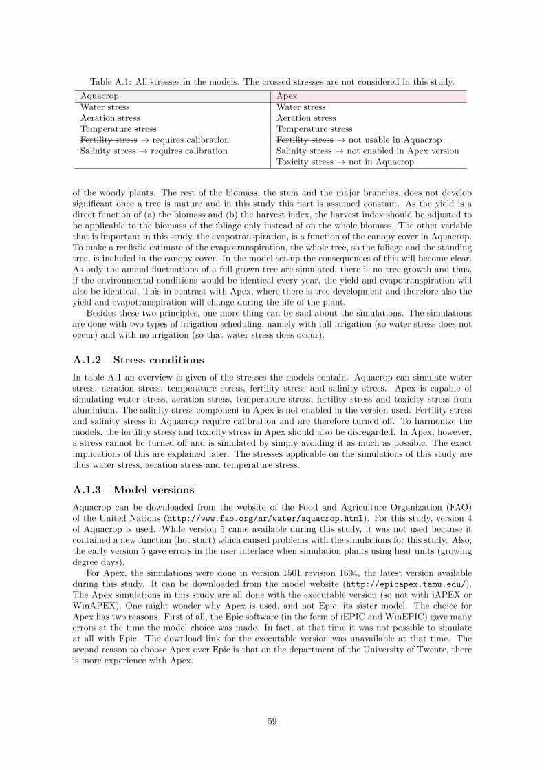
Table A.1: All stresses in the models. The crossed stresses are not considered in this study.

Aquacrop ApexWater stress Water stressAeration stress Aeration stressTemperature stress Temperature stressFertility stress → requires calibration Fertility stress → not usable in AquacropSalinity stress → requires calibration Salinity stress → not enabled in Apex version

Toxicity stress → not in Aquacrop

of the woody plants. The rest of the biomass, the stem and the major branches, does not developsignificant once a tree is mature and in this study this part is assumed constant. As the yield is adirect function of (a) the biomass and (b) the harvest index, the harvest index should be adjusted tobe applicable to the biomass of the foliage only instead of on the whole biomass. The other variablethat is important in this study, the evapotranspiration, is a function of the canopy cover in Aquacrop.To make a realistic estimate of the evapotranspiration, the whole tree, so the foliage and the standingtree, is included in the canopy cover. In the model set-up the consequences of this will become clear.As only the annual fluctuations of a full-grown tree are simulated, there is no tree growth and thus,if the environmental conditions would be identical every year, the yield and evapotranspiration willalso be identical. This in contrast with Apex, where there is tree development and therefore also theyield and evapotranspiration will change during the life of the plant.

Besides these two principles, one more thing can be said about the simulations. The simulationsare done with two types of irrigation scheduling, namely with full irrigation (so water stress does notoccur) and with no irrigation (so that water stress does occur).

A.1.2 Stress conditions

In table A.1 an overview is given of the stresses the models contain. Aquacrop can simulate waterstress, aeration stress, temperature stress, fertility stress and salinity stress. Apex is capable ofsimulating water stress, aeration stress, temperature stress, fertility stress and toxicity stress fromaluminium. The salinity stress component in Apex is not enabled in the version used. Fertility stressand salinity stress in Aquacrop require calibration and are therefore turned off. To harmonize themodels, the fertility stress and toxicity stress in Apex should also be disregarded. In Apex, however,a stress cannot be turned off and is simulated by simply avoiding it as much as possible. The exactimplications of this are explained later. The stresses applicable on the simulations of this study arethus water stress, aeration stress and temperature stress.

A.1.3 Model versions

Aquacrop can be downloaded from the website of the Food and Agriculture Organization (FAO)of the United Nations (http://www.fao.org/nr/water/aquacrop.html). For this study, version 4of Aquacrop is used. While version 5 came available during this study, it was not used because itcontained a new function (hot start) which caused problems with the simulations for this study. Also,the early version 5 gave errors in the user interface when simulation plants using heat units (growingdegree days).

For Apex, the simulations were done in version 1501 revision 1604, the latest version availableduring this study. It can be downloaded from the model website (http://epicapex.tamu.edu/).The Apex simulations in this study are all done with the executable version (so not with iAPEX orWinAPEX). One might wonder why Apex is used, and not Epic, its sister model. The choice forApex has two reasons. First of all, the Epic software (in the form of iEPIC and WinEPIC) gave manyerrors at the time the model choice was made. In fact, at that time it was not possible to simulateat all with Epic. The download link for the executable version was unavailable at that time. Thesecond reason to choose Apex over Epic is that on the department of the University of Twente, thereis more experience with Apex.

59

http://www.fao.org/nr/water/aquacrop.html

http://epicapex.tamu.edu/

A.1.4 Steps required to reproduce results

To recreate the results of this study it is recommended to follow the lines of this appendix. Thisimplies that one should start by creating the required climate data and setting it up for each of themodels. To acquire the reference evapotranspiration, which is derived from Apex, it is necessary toapply the general set-up first. After this, the general model parameters can be set and following thisthe location and plant specific parameters can be chosen for the required simulation. When one isnot familiar with Aquacrop, it is recommended to start with the tutorials available on the downloadwebsite. For Apex such tutorials are not available, but to get a feeling for this model one can use theuser guide to go through the different model components.

A.2 Setting up input

The forcing of the models is given by the climatic input and the parametrization of the soil. Forthe first one, a general description of the data with some small in depth clarifications for each of themodels is sufficient to recreate the data. For the soil data, both models are described separately.

A.2.1 Climate data

The climate files required for Aquacrop consist of five files; one main file (extension .CLI) and foursubfiles (.TMP, .PLU, .ETo and .CO2) from which the names are saved in the main file. Each ofthese subfiles contain climate variables on a daily basis. In Apex, there are two files; one file thatcontains all the daily climate variables (.DLY) and one that contains monthly values (.WP1).

The following climate variables are used in this study:

• Maximum temperature (daily)

• Minimum temperature (daily)

• Precipitation (daily)

• Solar radiation (daily)

• Reference evapotranspiration (daily)

• Atmospheric carbon dioxide concentration (yearly)

The first three climate variables are available from 1958 to 2010. Solar radiation and referenceevapotranspiration rates are available from 1981 to 2010. The carbon dioxide concentrations areavailable on a yearly basis from 1958 to 2014. Knowing this, the maximum simulation period is from1981 to 2010. The monthly average temperatures, precipitation and reference evapotranspiration foreach of the locations during the period 1981 to 2010 are visible in table A.2. Each of the climatevariables is explained below.

Maximum & minimum temperature and precipitation

The maximum temperature, the minimum temperature and the precipitation are all retrieved fromDe Graaf et al. (2014). From this global database, data is picked based on the longitude and latitudeof the location. The data is available from 1958 to 2010, although only the years 1981 to 2010 areused. Both models require daily values of these three variables. In addition, Apex requires alsomonthly values of them. More on the derivation of monthly data is explained at the end of thissection.

Solar radiation

Apex requires daily solar radiation data for the calculation of biomass. The model can also requirenet solar radiation for the evapotranspiration calculation, but the Hargreaves function that is usedin this study does not require this data (see appendix B).

60

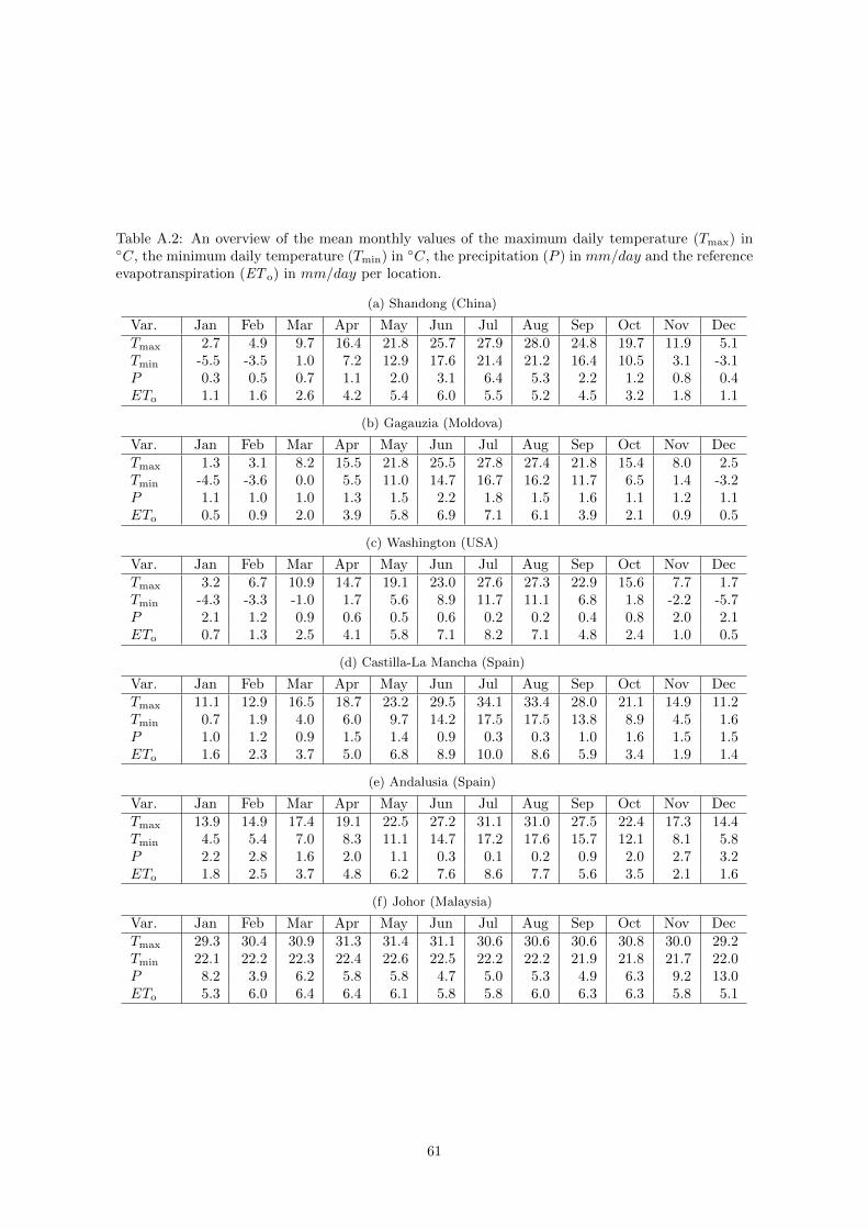
Table A.2: An overview of the mean monthly values of the maximum daily temperature (Tmax) in◦C, the minimum daily temperature (Tmin) in ◦C, the precipitation (P ) in mm/day and the referenceevapotranspiration (ET o) in mm/day per location.

(a) Shandong (China)

Var. Jan Feb Mar Apr May Jun Jul Aug Sep Oct Nov DecTmax 2.7 4.9 9.7 16.4 21.8 25.7 27.9 28.0 24.8 19.7 11.9 5.1Tmin -5.5 -3.5 1.0 7.2 12.9 17.6 21.4 21.2 16.4 10.5 3.1 -3.1P 0.3 0.5 0.7 1.1 2.0 3.1 6.4 5.3 2.2 1.2 0.8 0.4ETo 1.1 1.6 2.6 4.2 5.4 6.0 5.5 5.2 4.5 3.2 1.8 1.1

(b) Gagauzia (Moldova)

Var. Jan Feb Mar Apr May Jun Jul Aug Sep Oct Nov DecTmax 1.3 3.1 8.2 15.5 21.8 25.5 27.8 27.4 21.8 15.4 8.0 2.5Tmin -4.5 -3.6 0.0 5.5 11.0 14.7 16.7 16.2 11.7 6.5 1.4 -3.2P 1.1 1.0 1.0 1.3 1.5 2.2 1.8 1.5 1.6 1.1 1.2 1.1ETo 0.5 0.9 2.0 3.9 5.8 6.9 7.1 6.1 3.9 2.1 0.9 0.5

(c) Washington (USA)

Var. Jan Feb Mar Apr May Jun Jul Aug Sep Oct Nov DecTmax 3.2 6.7 10.9 14.7 19.1 23.0 27.6 27.3 22.9 15.6 7.7 1.7Tmin -4.3 -3.3 -1.0 1.7 5.6 8.9 11.7 11.1 6.8 1.8 -2.2 -5.7P 2.1 1.2 0.9 0.6 0.5 0.6 0.2 0.2 0.4 0.8 2.0 2.1ETo 0.7 1.3 2.5 4.1 5.8 7.1 8.2 7.1 4.8 2.4 1.0 0.5

(d) Castilla-La Mancha (Spain)

Var. Jan Feb Mar Apr May Jun Jul Aug Sep Oct Nov DecTmax 11.1 12.9 16.5 18.7 23.2 29.5 34.1 33.4 28.0 21.1 14.9 11.2Tmin 0.7 1.9 4.0 6.0 9.7 14.2 17.5 17.5 13.8 8.9 4.5 1.6P 1.0 1.2 0.9 1.5 1.4 0.9 0.3 0.3 1.0 1.6 1.5 1.5ETo 1.6 2.3 3.7 5.0 6.8 8.9 10.0 8.6 5.9 3.4 1.9 1.4

(e) Andalusia (Spain)


(f) Johor (Malaysia)


61

According to Allen et al. (1998), the extraterrestrial daily solar radiation can be calculated ac-cording to the latitude and the day of the year. Following the symbols used by Allen et al. (1998),this looks like the equation

Ra = f(J, ϕ), (A.1)

wherein Ra [MJ/m2/day] is the extraterrestrial solar radiation, J [−] the day in the year and ϕ [◦] thelatitude in decimal degrees. In reality, not all of this radiation will reach the earth. This because ofclouds, dust, humidity etcetera. For Apex, the net solar radiation is required, which is the radiationcorrected for all these factors. The equation for this radiation looks like

Rs =(as + bs ·

n

N

)·Ra, (A.2)

in which Rs [MJ/m2/day] is the solar radiation and as [−] the fraction of the radiation that wouldreach the earth if the sky is covered the whole day with clouds. bs [−] is the fraction of radiationthat reaches the earth surface if there is a clear sky during a certain period of the day. This perioddepends on n [hours], the amount of sunshine hours on a day and N [hours], the maximum amountof sunshine hours on a day. This last one is also a function of the day of the year and the latitude.The amount of sunshine hours n is obtained from Era Interim and is available from 1981 to 2010(Dee et al., 2011).

Reference evapotranspiration

The reference evapotranspiration, required by Aquacrop, is calculated with Apex. At each of thelocations, the temperature, precipitation and solar radiation is set-up. The resulting potential eva-potranspiration is considered as the reference evapotranspiration for Aquacrop. More on this inappendix B. The set-up of the model during these simulations is as the general set-up (see sectionA.3). A few changes are made. The albedo of the soil is chosen as 0.23 (Allen et al., 2006). The plantsimulated is summer pasture, in combination with a land use number of 22, although this does notchange the results of the potential evapotranspiration. The sowing date is the first day of January inthe first year, which is 1981. The simulation runs from 1981 to 2010.

Atmospheric carbon dioxide concentration

There are also yearly atmospheric carbon dioxide (CO2) concentrations required by the models. Bothmodels have an embedded database of global atmospheric concentrations, but these databases arenot the same. As the CO2 concentrations of Aquacrop are better accessible, these concentrations areused in both models. The CO2 concentrations in Aquacrop are the atmospheric concentrations atMauna Loa (Hawaii).

To put the carbon dioxide concentration of Aquacrop in Apex, there are a few complications.The way Apex reads the CO2 concentration is namely not straightforward. When the model findsa CO2 concentration on a specific date, it only starts using it the year following this date. So the

Table A.3: The global atmospheric carbon dioxide concentrations (in parts per million) for each ofthe years.

Year concentration Year concentration Year concentration1981 340.11 1991 355.48 2001 371.131982 341.22 1992 356.27 2002 373.221983 342.84 1993 356.95 2003 375.771984 344.40 1994 358.63 2004 377.491985 345.87 1995 360.62 2005 379.801986 347.19 1996 362.37 2006 381.901987 348.98 1997 363.47 2007 383.771988 351.45 1998 366.50 2008 385.591989 352.89 1999 368.14 2009 387.371990 354.16 2000 369.41 2010 389.85

62

concentration entered on the first of January 1990 will be used as the CO2 concentration in 1991.Knowing this, the CO2 concentration for a specific year should be entered in the year before. For thefirst year, the model uses the CO2 parameter (called CO2) in the control file of Apex. The value for1981 is entered at this location. An overview of the concentrations for each of the years can be foundin table A.3.

Deriving monthly data

Both models require daily climate files. In addition, Apex also requires a monthly climate file. Theaverage monthly values for the maximum temperature, minimum temperature and solar radiationcan be derived by summing up the values per month and taking the average of this. This will resultin the values that are also present in table A.2. The standard deviation can be calculated easily fromthis list of all values per month.

The average monthly precipitation can be calculated similarly. The number of rainy days permonth can be calculated from the list by taking the total number of rainy days for the whole period1981 to 2010 and divide this by the length of the period (30 years). The rest of the variables in themonthly weather file are left at zero, because the model documentation of Apex states that this canbe left zero. An example of a monthly weather file of Apex is given in figure A.3.

A.2.2 Soil parametrization

While the climatic input is identical in the models, the soil parametrization is to a certain extentdifferent. What the models do have in common is that the soil parametrization is in both casesderived from De Lannoy et al. (2014). They provide a global map with 253 different soil types, eachof them representing a soil structure that consists of two layers with a thickness of 0.30 and 0.70meter, with different values for soil parameters per layer. The soil types per location are acquiredon a similar method as the climate data; based on the longitude and latitude the soil type is pickedfrom the global database. For each of the models, the soil structure is further explained below. Thesoil types from De Lannoy et al. (2014) that are used in this study are given in table A.4.

Aquacrop soil

The parametrization of Aquacrop consists of the soil file itself (.SOL), a file containing the initial soilwater content (.SW0) and a file with the groundwater characteristics (.GWT). In the first one thereare four general soil parameters that need to be set: the curve number, the readily evaporable water

Shandong

119.16 35.56

2.69 4.89 9.73 16.44 21.80 25.70 27.91 27.96 24.84 19.67 11.86 5.08

-5.54 -3.48 1.02 7.20 12.90 17.63 21.43 21.17 16.45 10.53 3.12 -3.14

3.14 3.56 3.60 3.56 3.22 2.60 2.20 2.02 2.53 3.38 4.20 3.67

3.02 3.42 3.47 3.48 3.07 2.48 2.12 2.06 2.48 3.40 4.12 3.55

9.86 15.02 20.20 33.40 59.99 92.44192.94159.10 67.38 34.77 24.11 10.75

0.00 0.00 0.00 0.00 0.00 0.00 0.00 0.00 0.00 0.00 0.00 0.00

0.00 0.00 0.00 0.00 0.00 0.00 0.00 0.00 0.00 0.00 0.00 0.00

0.00 0.00 0.00 0.00 0.00 0.00 0.00 0.00 0.00 0.00 0.00 0.00

0.00 0.00 0.00 0.00 0.00 0.00 0.00 0.00 0.00 0.00 0.00 0.00

2.73 3.67 4.00 4.87 6.60 8.73 16.87 16.27 7.13 5.03 3.90 2.77

0.00 0.00 0.00 0.00 0.00 0.00 0.00 0.00 0.00 0.00 0.00 0.00

13.60 16.00 18.41 19.95 19.80 19.78 19.73 19.69 18.41 15.98 13.59 12.61

0.00 0.00 0.00 0.00 0.00 0.00 0.00 0.00 0.00 0.00 0.00 0.00

0.00 0.00 0.00 0.00 0.00 0.00 0.00 0.00 0.00 0.00 0.00 0.00

Figure A.3: An example of a monthly weather file of Apex. Here the climate file of Shandong isshown. The first two lines contain comments and are not used by the model.

63

Table A.4: The soil types for each of the locations, including their sand, clay and silt content. Thesoil code refers to the one of De Lannoy et al. (2014).

Plant Topsoil (Sa% / Cl% / Si%) Subsoil (Sa% / Cl% / Si%)Apple tree (Sh) 224 (46.67 / 16.67 / 36.67) 55 (53.33 / 13.33 / 33.33)Apple tree (Ga) 186 (13.33 / 43.33 / 43.33) 186 (13.33 / 43.33 / 43.33)Apple tree (Wa) 224 (46.67 / 16.67 / 36.67) 40 (43.33 / 23.33 / 33.33)Grapevine 210 (33.33 / 23.33 / 43.33) 126 (33.33 / 23.33 / 43.33)Olive tree 185 (16.67 / 46.67 / 36.67) 16 (23.33 / 43.33 / 33.33)Oil palm 207 (46.67 / 26.67 / 26.67) 110 (36.67 / 36.67 / 26.67)

Table A.5: An overview of some important soil parameter values for the .SOL file of Aquacrop.

Plant cn [−] REW [mm] Soil class CRa [−] CRb [−]Apple tree (Sh) 34 8 I Sandy -0.3143 -0.1072Apple tree (Ga) 77 11 IV Silty clayey -0.4967 1.7307Apple tree (Wa) 58 8 II Loamy -0.4772 0.4829Grapevine 58 9 II Loamy -0.4751 0.5273Olive tree 71 11 III Sandy clayey -0.5738 -0.7387Oil palm 71 8 III Sandy clayey -0.5749 -0.6456

from the top layer, the number of soil horizons and the depth of the restrictive layer. First of all, thecurve number is set equal to the curve number Apex calculates. The values of these curve numberscan be found in table A.5 and are retrieved in the same run as the potential heat units (more onthese runs in section A.4.1). The readily evaporable water, or REW , is calculated by the equationgiven in the manual of the model. This equation is

REW = 0.4(θFC − 0.5 · θWP), (A.3)

in which REW [mm] is the readily evaporable water, θFC [mm] the field capacity and θWP [mm]the wilting point. This equation is applied on the topsoil layer only, resulting in a certain amount ofREW . This REW is entered as an integer in the soil file. The values for the readily available waterare shown in table A.5. There are two soil horizons, as described by De Lannoy et al. (2014). Thereis no restrictive soil layer, resulting in a value for this parameter of -9.

Besides the general soil parameters there are also layer specific parameters in the soil file ofAquacrop. The thickness of the layer (in the file called Thickness), the soil moisture content atsaturation (Sat), the field capacity (FC), the wilting point (WP) and the saturated hydraulic con-ductivity (Ksat) are all given by De Lannoy et al. (2014). This means that there are two parametersleft, namely the capillary rise parameters a (CRa) and b (CRb). As this study does not considers agroundwater table, the values for these parameters do not influence the results. The capillary riseparameters used in this study are given in table A.5. The soil classes, which were important for thecalculation of capillary rise, are still important for Apex. The class is determined using the methodin the documentation of Aquacrop. This means that based on the soil moisture content at saturation,the field capacity and the wilting point, all of the bottom layer only, the soil class is determined. Ifmultiple classes can occur given these three parameters, the highest class is chosen.

Next to the soil file, Aquacrop also requires a file that contains the initial conditions of the soil(.SW0). This file also consists of general soil parameters and layer specific parameters. In the generalsoil file, only the number of soil layers is filled in (2), while the water stored between soil bunds, theelectrical conductivity and the soil water content for specific layers are all put to zero. In the layerparameters, the thickness of each of the layers and the initial water content need to be set. Thethickness of the first layer is 0.30 m and the thickness of the second layer is 0.70 m. The initial watercontents are equal to the field capacities of the layers. The electrical conductivity (EC e) is set tozero.

In Aquacrop, a groundwater table can be set with the groundwater file. As said, no groundwateris simulated in this study. In the project file (.PRM), explained in section A.3, the name for thegroundwater file is set to ’(None)’.

64

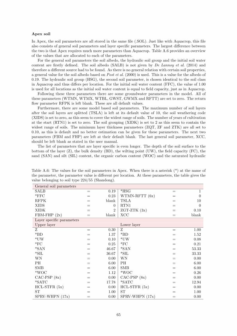
Apex soil

In Apex, the soil parameters are all stored in the same file (.SOL). Just like with Aquacrop, this filealso consists of general soil parameters and layer specific parameters. The largest difference betweenthe two is that Apex requires much more parameters than Aquacrop. Table A.6 provides an overviewof the values that are allocated to each of the parameters.

For the general soil parameters the soil albedo, the hydraulic soil group and the initial soil watercontent are firstly defined. The soil albedo (SALB) is not given by De Lannoy et al. (2014) andtherefore a different source had to be found. As there is no general relation with certain soil properties,a general value for the soil albedo based on Post et al. (2000) is used. This is a value for the albedo of0.19. The hydraulic soil group (HSG), the second soil parameter, is chosen identical to the soil classin Aquacrop and thus differs per location. For the initial soil water content (FFC), the value of 1.00is used for all locations as the initial soil water content is equal to field capacity, just as in Aquacrop.

Following these three parameters there are some groundwater parameters in the model. All ofthese parameters (WTMN, WTMX, WTBL, GWST, GWMX and RFTT) are set to zero. The returnflow parameter RFPK is left blank. These are all default values.

Furthermore, there are some model based soil parameters. The maximum number of soil layersafter the soil layers are splitted (TSLA) is left at its default value of 10, the soil weathering code(XIDS) is set to zero, as this seem to cover the widest range of soils. The number of years of cultivationat the start (RTN1) is set to zero. The soil grouping (XIDK) is set to 2 as this seem to contain thewidest range of soils. The minimum layer thickness parameters (ZQT, ZF and ZTK) are all set to0.10, as this is default and no better estimation can be given for these parameters. The next twoparameters (FBM and FHP) are left at their default blank. The last general soil parameter, XCC,should be left blank as stated in the user manual.

The list of parameters that are layer specific is even longer. The depth of the soil surface to thebottom of the layer (Z), the bulk density (BD), the wilting point (UW), the field capacity (FC), thesand (SAN) and silt (SIL) content, the organic carbon content (WOC) and the saturated hydraulic

Table A.6: The values for the soil parameters in Apex. When there is a asterisk (*) at the name ofthe parameter, the parameter value is different per location. At these parameters, the table gives thevalue belonging to soil type 224/55 (Shandong).

General soil parametersSALB = 0.19 *HSG = 1*FFC = 0.23 WTMN-RFTT (6x) = 0RFPK = blank TSLA = 10XIDS = 0 RTN1 = 0XIDK = 2 ZGT-ZTK (3x) = 0.10FBM-FHP (2x) = blank XCC = blankLayer specific parametersUpper layer Lower layerZ = 0.30 Z = 1.00*BD = 1.37 *BD = 1.52*UW = 0.10 *UW = 0.08*FC = 0.25 *FC = 0.21*SAN = 46.67 *SAN = 53.33*SIL = 36.67 *SIL = 33.33WN = 0.00 WN = 0.00PH = 6.00 PH = 6.00SMB = 6.00 SMB = 6.00*WOC = 1.12 *WOC = 0.26CAC-PSP (8x) = 0.00 CAC-PSP (8x) = 0.00*SATC = 17.78 *SATC = 12.94HCL-STFR (5x) = 0.00 HCL-STFR (5x) = 0.00ST = 1.00 ST = 1.00SPRV-WHPN (17x) = 0.00 SPRV-WHPN (17x) = 0.00

65

conductivity (SATC) are all found in De Lannoy et al. (2014). The initial soil water storage (ST)is set equal to the field capacity, which results in a parameter value of one (as this is the fractionof field capacity). The parameters that describe the pH of the soil (PH and SMB) are both set to6. The pH is important for the aluminium stress and to avoid this stress it is necessary that thesevalues are higher than 5.6. The rest of the parameters, all 31, are left at zero because (a) no valuesare available for these parameters and the documentation states that they can be left at zero or (b)the values for these parameters do not change the results.

A.3 Model set-up

The general set-up of the models is explained in this section. The general set-up refers to theparametrization of the models that does not change over the years, the plants, the locations or thetype of simulation (irrigated or rainfed). For each of the models this set-up is explained below.To value the parameters there is no general source available as it was for the soil parametrization.Therefore, a best guess is made for each of the parameters. When this is not possible, the defaultvalue is assumed to be representative.

A.3.1 Aquacrop

The simulations in Aquacrop are run through multiple run project files (.PRM files). Such a filecan be seen as the main file that contains the program parameters and contains links to all subfiles.Each of these subfiles also contains parameters for a component of the model. These subfiles are theclimate files (with the extensions .CLI, .TMP, .ETo, .PLU and .CO2), the soil files (.SOL, .SW0 and.GWT), the plant file (.CRO) and some management files (.IRR, .MAN and .OFF). The climate filesand the soil files are already discussed in section A.2. The rest of the files are discussed here. Anoverview of all the parameters is given in table A.7.

Plant file (.CRO)

The plant file contains all the plant specific parameters. It is not surprising that a lot of theseparameters can not be considered as general parameters, but depend on the plant being simulated.These plant specific parameters are given in table A.7a. These contain all the parameters that describethe plant growth as a function of heat units (or growing degree days), the minimum temperature theplant needs for growing, the crop coefficient, the depth of the roots, the maximum canopy cover, theminimum canopy cover (function of the planting density) and the harvest index. The values for theseparameters are explained in section A.4.

In the plant file there are also parameters that can be set for all simulations. First of all, the plantis sown, although this will not lead to different results in respect to a transplanted plant. The plantdevelopment is set in heat units (GDD), corresponding to Apex which also has heat units underlyingthe simulation. The upper temperature is set to 40 ◦C. The reason that this is a general parameterand not a plant specific parameter has to do with the fact that this temperature is only relevant forthe accumulation of heat units. For the temperature stress, the model uses the parameters ’minimumand maximum air temperature for pollination’ and the ’minimum growing degree days required forfull biomass production’. This last one is a plant specific parameter, the first two not. The valueof 40 ◦C is chosen as this is in non of the locations ever reached as the mean daily temperature. Inthis way, the heat unit equation from Aquacrop becomes exactly the same as the one of Apex. Seeequation A.4 and A.5 later in this appendix.

After the temperature, there are five parameters that describe the response of different plantcomponents to the soil fertility and salinity. These parameters are all set to 25, which means thatthese stresses are turned off. Also the electrical conductivity parameters are turned off, resulting ina value of -9. The soil cover per plant is 200 cm2. The model uses this, together with the number ofplants per hectare (plant specific parameter), to determine the initial canopy cover. Therefore one ofthese two parameters can be fixed, while the other one determines per plant. The plant determinacyis linked with flowering.

For the adjusted parameters, there is one parameter remaining. As can be seen, the amount ofheat units (GDD) to emergence is set on -1. For a correct simulation of evapotranspiration, it isimportant to keep the canopy cover intact in the winter (more on this is section A.4.2). Aquacrop

66

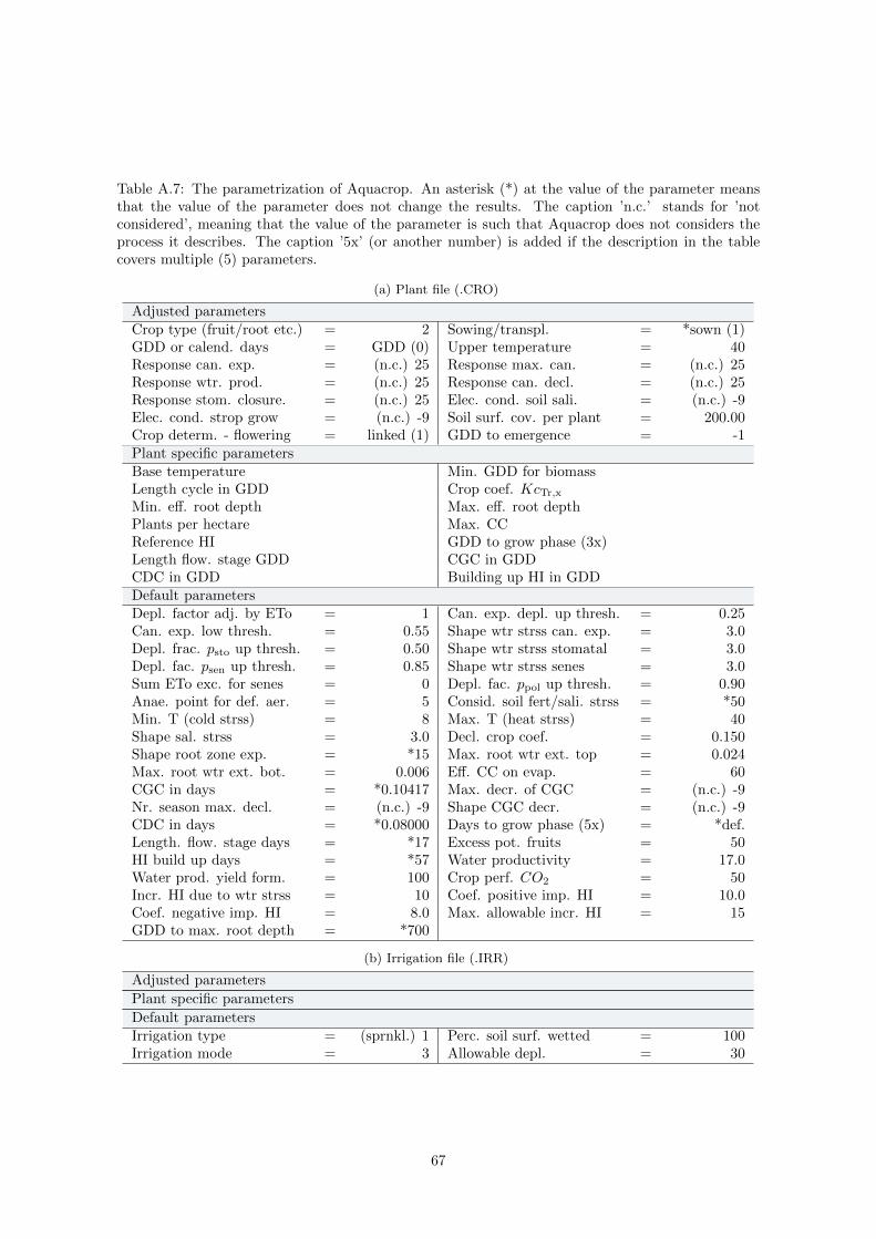
Table A.7: The parametrization of Aquacrop. An asterisk (*) at the value of the parameter meansthat the value of the parameter does not change the results. The caption ’n.c.’ stands for ’notconsidered’, meaning that the value of the parameter is such that Aquacrop does not considers theprocess it describes. The caption ’5x’ (or another number) is added if the description in the tablecovers multiple (5) parameters.

(a) Plant file (.CRO)

Adjusted parametersCrop type (fruit/root etc.) = 2 Sowing/transpl. = *sown (1)GDD or calend. days = GDD (0) Upper temperature = 40Response can. exp. = (n.c.) 25 Response max. can. = (n.c.) 25Response wtr. prod. = (n.c.) 25 Response can. decl. = (n.c.) 25Response stom. closure. = (n.c.) 25 Elec. cond. soil sali. = (n.c.) -9Elec. cond. strop grow = (n.c.) -9 Soil surf. cov. per plant = 200.00Crop determ. - flowering = linked (1) GDD to emergence = -1Plant specific parametersBase temperature Min. GDD for biomassLength cycle in GDD Crop coef. KcTr,x

Min. eff. root depth Max. eff. root depthPlants per hectare Max. CCReference HI GDD to grow phase (3x)Length flow. stage GDD CGC in GDDCDC in GDD Building up HI in GDDDefault parametersDepl. factor adj. by ETo = 1 Can. exp. depl. up thresh. = 0.25Can. exp. low thresh. = 0.55 Shape wtr strss can. exp. = 3.0Depl. frac. psto up thresh. = 0.50 Shape wtr strss stomatal = 3.0Depl. fac. psen up thresh. = 0.85 Shape wtr strss senes = 3.0Sum ETo exc. for senes = 0 Depl. fac. ppol up thresh. = 0.90Anae. point for def. aer. = 5 Consid. soil fert/sali. strss = *50Min. T (cold strss) = 8 Max. T (heat strss) = 40Shape sal. strss = 3.0 Decl. crop coef. = 0.150Shape root zone exp. = *15 Max. root wtr ext. top = 0.024Max. root wtr ext. bot. = 0.006 Eff. CC on evap. = 60CGC in days = *0.10417 Max. decr. of CGC = (n.c.) -9Nr. season max. decl. = (n.c.) -9 Shape CGC decr. = (n.c.) -9CDC in days = *0.08000 Days to grow phase (5x) = *def.Length. flow. stage days = *17 Excess pot. fruits = 50HI build up days = *57 Water productivity = 17.0Water prod. yield form. = 100 Crop perf. CO2 = 50Incr. HI due to wtr strss = 10 Coef. positive imp. HI = 10.0Coef. negative imp. HI = 8.0 Max. allowable incr. HI = 15GDD to max. root depth = *700

(b) Irrigation file (.IRR)

Adjusted parameters

Plant specific parameters

Default parametersIrrigation type = (sprnkl.) 1 Perc. soil surf. wetted = 100Irrigation mode = 3 Allowable depl. = 30

67

Table A.7: (continued) The parametrization of Aquacrop. An asterisk (*) at the value of the param-eter means that the value of the parameter does not change the results. The caption ’n.c.’ stands for’not considered’, meaning that the value of the parameter is such that Aquacrop does not considersthe process it describes. The caption ’5x’ (or another number) is added if the description in the tablecovers multiple (5) parameters.

(c) Project file (.PRM)

Adjusted parametersDefault meth. GDD calc. = 1 CN with AMC = 0Plant specific parametersDates simulation & plant Soil evap. coeff. (Kex)Default parametersEvap. decl. factor = 4 Thresh. CC below HI = 5Start depth root zone = 70 Max. allowable root zone = 5.00Shape water strss - root = -6 Req. swc for germin. = 20Adj. factor SW depl. = 1.0 Nr. days aeration = 3Exp. of senesc. = 1.00 Decr. of psen = 12Thresh. water strss - sal. = 0 Depth affect. by evap = 30Consid. depth for CN = 0.30 Salt. diff. factor = 20Salt solubility = 100 Shape factor. SWC - CR = 16Default min. T = 12.0 Default max. T = 28.0

simulates every plant as if it is an herbaceous one, meaning that the plant dies at harvest. To keepthe canopy cover intact, the plant of the following year should have a canopy cover from the firstday it grows, which is the day after harvest of the previous plant. To reach this, it is required to setthe heat units for emergence to minus one. See figure A.4. Setting it to zero will namely lead to theproblem that if the moment of harvest occurs in winter, when no heat units are acquired, the plantwill not emerge until the first moment that heat units are acquired. As this can take months, this

1984 1985 1986 1987

10

30

50

70

90

Can

opycover[m

2/m

2]

GDD to emergence: 0

GDD to emergence: -1

(a) Canopy cover 1984-1986 in Gagauzia

1984 1985 1986 19870

5

10

15

20

25

Heatunits[◦C] Heat units per day

(b) Heat units 1984-1986 in Gagauzia

Figure A.4: The dependency of the plant development on the heat units to emergence. The top plotshows the heat to emergence set as zero or minus one. The bottom plot shows the heat units itself.As can be seen, instant emergence only occurs with a value of minus one.

68

would mean that the canopy cover can be zero during a few months of the year. To avoid this, theamount of heat units to emergence is set to -1.

The rest of the parameters in the plant file are all left at default. These parameters are alsoshown in table A.7a. The parameters are not adjusted because there is simply no better estimateavailable for them. There are a few parameters that may require some additional clarification. Tostart with, the minimum (8 ◦C) and maximum (40 ◦C) temperature at which pollination start to failfrom cold and heat stress, are left at their default. This seems quite unlikely, because the temperaturea plant flourished best in depends strongly on the plant. While this is true, there are simply no betterestimates available for these specific parameters. It is assumed that the values given by Aquacrop areconservative for a wide range of plants. The plant specific temperature characteristics are coveredby the accumulation of heat units and the minimum amount of heat units required for biomassproduction.

A second parameter that requires clarification is the shape factor for the soil salinity stress. Thisis set at 3.0, its default value which describes a convex shaped relation between the salinity stresscoefficient and the electrical conductivity of the soil. As salinity stress is turned off, the shape of thisrelation should not matter. However, a comparison between the results of simulations with differentvalues for this shape (convex shape of 3.0 and linear shape of 0.0) show that the result do change. Infigure A.5, these results are shown for the biomass and the transpiration. The reason for the differenceis unclear, as the electrical conductivity threshold are both set to -9. Even when setting the electricalconductivity to values which would in practice never be reached, the model still responses to thedifferent values of this shape parameter. As the exact reason for this still remains unclear, the valuefor this parameter is left at its default.

The rest of the parameters describe a wide range of processes in the model. Some of them do notchange the results at all, others only slightly and some even a lot. All of these remaining parametersare left at their default value.

Feb 1982 May 1982 Aug 1982 Nov 19820

1.5

3.0

4.5

Biomass[ton

/ha] Convex shaped salinity relation

Linear shaped salinity relation

(a) Biomass 1982 in Gagauzia

Feb 1982 May 1982 Aug 1982 Nov 19820

1.5

3.0

4.5

Transpiration[m

m]

Convex shaped salinity relation

Linear shaped salinity relation

(b) Transpiration 1982 in Gagauzia

Figure A.5: The dependency of the plant development on the shape relation between the salinitystress coefficient and the electrical conductivity of the soil. While salinity stress is turned off, theshape of the relation described by the parameter value of 3.0 (convex) and 0.0 (linear) still changesthe results.

69

Management files (.IRR, .MAN and .OFF)

From the management files, only the irrigation file is used. This means that other managementoptions, described by the .MAN file and the .OFF file, are not considered. For situations that requireirrigation, the default irrigation file (Inet.IRR) is used. The characteristics of this file are shown infigure A.7b.

Project file (.PRM)

Finally Aquacrop has a project file, which can be considered as the master file from which thesimulation is run. This file firstly contains, for every year in the file, the start and end date of thesimulation and the start and end date of the cropping period. While these are important, they areplant, year and location specific. These dates are therefore discussed in section A.4.

Besides these dates, the project file also contains the program parameters. The values for theseparameters for the simulations in this study are given in table A.7c. As can be seen here, most ofthe program parameters are left at their default value. This is mainly caused by the fact that theseprogram parameters are very model specific and there are no general methods available to estimatethem.

There are two program parameters that are adjusted. First of all, the method to calculate the heatunits (GDD) is adjusted to type 1. From the three methods available in Aquacrop, this method liesclosest to the heat unit equation of Apex. This method of Aquacrop, which is given by the function


2− Tbase; 0 ≤ HU (i) ≤ Tupper − Tbase, (A.4)

is the same as the equation in Apex, which is


2− Tbase; 0 ≤ HU (i). (A.5)

as long as Tupper is never reached. As can be seen in table A.7a, this upper threshold is set to 40 ◦C,a temperature that in practice is never reached. In this way, the heat unit calculations are equal forboth models. Note that equations A.4 and A.5 contain the symbols used in this document and notthe original symbols in the manuals of the respective models.

Also the curve number method is adjusted. In this study, it is chosen to work with a constant curvenumber in both models. Therefore, the program parameters describing this is adjusted. Furthermore,there is one parameter, the soil evaporation coefficient, which is plant dependent and is therefore notgiven here. More on this parameter can be found in section A.4.

A.3.2 Apex

In Apex the number of files for the simulation is rather large. To get a good overview of the files, fourfile types are distinguished in this appendix. First of all there are input files, consisting of the dailyweather file (.DLY), the monthly weather file (.WP1) and the soil file (.SOL). These are all explainedin the input section A.2. Furthermore, run files, database files and a print file are distinguished. Inthis report, database files are considered as all the files that contain a long list of different options auser can select from. For example, one can think of the plant database, from which a user can specifywhich plant it wants to use. Also the files that contain all the different default weather stations areconsidered database files. The run files are all the files that control the simulation. These includethe files that state which operation is performed and when, at which date the simulation starts, whatthe program parameters are etcetera. And finally there is a print file, which does not control thesimulation itself, but only influences the output that is being displayed. In this study at least thedaily evapotranspiration and the yearly yield values should be printed. The database and run filesare discussed below. Note that only the files used during the simulations in this study are mentioned.Some files, such as herd files, are not used in this study and are therefore also not discussed here.Furthermore, it is important to know that the names given with each of the files are the defaultnames; a user might have different names for the files.

70

Crop 1 2 3 4 5 6 7 8 9 10...

# NAME WA HI TOP TBS DMLA DLAI DLAP1 DLAP2 RLAD RBMD...

1 SOYB 25.00 0.30 25.00 10.00 5.00 0.90 15.05 50.95 0.10 1.00...

2 CORN 40.00 0.50 25.00 8.00 6.00 0.80 15.05 50.95 1.00 1.00...

3 GRSG 37.00 0.50 27.50 10.00 5.50 0.80 15.01 60.95 0.50 0.50...

4 COTS 25.00 0.60 27.50 12.50 6.00 0.95 15.01 50.95 0.50 0.50...

5 COTP 25.00 0.40 27.50 12.50 6.00 0.95 15.01 50.95 0.50 0.50...

6 PNUT 30.00 0.00 25.00 9.00 5.00 0.85 15.01 50.95 1.00 0.50...

7 SUNF 49.00 0.30 25.00 10.00 5.00 0.55 15.01 50.95 1.00 2.00...

......

(a) The plant file (CROP.DAT)

1 1.WP1 32.41 -99.68 545.6 TX_ABILENE_RGNL_AP

2 2.WP1 32.73 -99.3 426.7 TX_ALBANY

3 3.WP1 32.75 -99.85 520.3 TX_ANSON_3ESE

4 4.WP1 33.6 -98.61 321.2 TX_ARCHER_CITY_1E

5 5.WP1 32.74 -97.13 199.6 TX_ARLINGTON

6 6.WP1 32.16 -95.83 136.5 TX_ATHENS

7 7.WP1 30.32 -97.76 204.2 TX_AUSTIN-CAMP_MABR

8 8.WP1 32.26 -96.64 140.5 TX_BARDWELL_DAM

9 9.WP1 28.46 -97.71 77.7 TX_BEEVILLE_5_NE

......

(b) The monthly weather list file (WPM1.DAT)

Figure A.6: Example of the two different Apex database files. The plant file and the monthly weatherfile are shown. The first contains a list of options a user can choose from, the second contains a listof subfiles a user has to choose from. Only the first 9 lines are shown.

Database files

There are two different types of files within the category database files, see figure A.6. First of all, onecan identify the tillage file (TILL.DAT), the plant file (CROP.DAT), the fertiliser file (FERT.DAT)and the pesticide file (PEST.DAT). Each of these files provides a list of options a user can choose fromin one of the run files. Attached to each of the options is a list of parameters that the model requires.See figure A.6a. It is worth mentioning that non of the parameters in these files are changed. In theplant file one file is added (oil palm).

Within database files, also list files can be distinguished. These are the Apex site list (SITE.DAT),the subarea list (SUB.DAT), the soil list (SOIL.DAT), the operation list (OPS.DAT), the dailyweather list (WDLST.DAT) and the monthly weather list (WPM1.DAT). Similar as with the otherdatabase files, a user also chooses from a list file. But here an option does not contain parameters ofits own, but only refer to a file. See figure A.6b. In these list files, it is important that the subfilesused in the simulation are added to the list. For example, in the soil list, the name of the soil usedin the simulation should be added. For the list of the daily weather file and the monthly weather filealso the longitude, latitude and height (0.0 m) are entered.

Run files

Within the run files, the most important file for the simulation is the master file (APEXFILE.DAT).This file is comparable with the project file of Aquacrop and contains a list of subfiles that are requiredfor the simulation. While this file is crucial for the simulation, it is not important to mention broadlyhere, as nothing is changed in this file. When a user changes file names for the simulation it can benecessary to adjust this master file.

Another important run file is the parameter file (PARMS.DAT). The parameters within this fileare to some extent similar to the program parameters of Aquacrop. It contains the most coefficientfor equations and S-curves. As stated in the documentation of the model, these parameters shouldonly be changed in agreement with the model developers. As no better estimates are available forany of the over 150 parameters in this file and because of the warning given in the documentation,

71

none of the parameters are changed.The dimensions file (APEXDIM.DAT) sets the maximum allowable range of certain operations.

One can think of the maximum number of years a user can specify operations. They do not directlyinfluence the results, but it is important that the dimensions are set large enough so that all thesimulations can be done. In practice this means that the number of years that operations can bespecified should be at least 30.

Until so far the files discussed are not changed a lot. There are however five files that need moreclarification. These are the run file (APEXRUN.DAT), the control file (APEXCONT.DAT), thesubarea file (.SUB), the operations file (.OPS or .OPC) and the site file (.SIT). The parameters foreach of these files are given in table A.8. Each of the files is discussed further below.

The run file contains seven parameters, from which four (ISIT, IWPN, IWND and ISUB) onlyrefer to a subfile in one of the list files. For these, it is important that the corresponding subfilematches the one required for the simulation. The reference to the wind file (IWND) is not important,as no wind is considered in the simulations of this study. The parameter ISOL is set to zero, as thisrefers to a normal run (in contrast with using a .SOT file). The storm parameter IRFT is also set tozero; storms are not considered. Finally, ASTN is simply the name which is given to the output files.One can choose every name here that is convenient.

The control file is more comprehensive than the run file. First of all, it contains the length of thesimulation (NBYR) and the start date (IYR, IMO, IDA). The input code (NGN) should be enteredsuch that it contains precipitation, the maximum and minimum temperature and the solar radiation(therefore code 123). The estimation of the curve number (ISCN) is set to deterministic instead ofstochastic. The precipitation code is set such that it represents normal conditions (no tropical stormsor extreme droughts). A normal soil erosion is chosen (ISTA), because the static soil will not containany carry over effects of the soil through the years. Identical to the choice made in Aquacrop, thecurve number method is set constant in this model (NVCN). The carbon dioxide concentration (ICO2)is set as input, with an initial concentration of 340.11 parts per million (CO2). More information onthis is found in section A.2.1. The latitude is input, affecting the parameter IAZM. The final adjustedparameters are concerned with the vertical and horizontal pipe flow parameters (CPV0 and CPH0).These are both set to zero, meaning that pipe flow does not occur in either direction. The rest of theparameters are left at their default value.

The next important of the run files is the subarea file. This file contains plant specific parameters,general parameter and parameters which are left at their default, as can be seen in table A.8c. Thefirst plant specific parameter is the soil number that is picked from the soil list (INPS). This changesper location. While the same can be said about the climate files (part of the general parameters,parameter IWTH), this study uses climate data such that the climate file is overwritten per location.A user can of course choose to also overwrite the soil file for every location or to create differentclimate files for each location.

There are three more plant specific parameters. The first two are the latitude (YCT) and longitude(XCT). The last one is the irrigation code (BIR). This last parameter describes at which amountof water stress automatic irrigation occurs. A parameter value for BIR of 1 means that the modelirrigates as soon as even a little water stress occurs, while a parameter value of 0 means that noautomatic irrigation is applied what so ever. Depending on the type of irrigation, the parameter isset to 1 if water stress is to be avoided and set at 0 if water stress is allowed.

For the general set-up in the subarea file, the parameters IOPS and IWTH describe the operationfile and the climate file that are considered. The NVCN parameter is also in this file; the samevalue is given as in the control file. The parameter for the land use number (LUNS), which is set inthe operation file (explained below) can be overwritten here. By setting it to zero this is avoided.The upland slope (SLP) is set to zero to avoid horizontal flow components. The irrigation scheduling(NIRR) is set to flexible, such that automatic irrigation can occur based on the stress that is measured.The irrigation type (IRR) is set to sprinkler irrigation. There is no minimum time between irrigationor fertiliser application (IRI and IFA). The parameter IDR allows for the simulation of drainage pipes,but as this is not in Aquacrop, the simulation of them is avoided by setting the parameter to zero.The effectiveness of the irrigation is set with the parameter EFI, which simply states the fraction ofthe irrigation that becomes runoff. In this study this is set to zero (no over-irrigation). Runoff canof course still occur due to rainfall. The parameters for setting the minimum and maximum amountof irrigation of a single event or a year (VIMX, ARMN and ARMX) are all set to zero, meaningthat there is no minimum or maximum. The factor BFT is the fertiliser equivalent of the irrigation

72

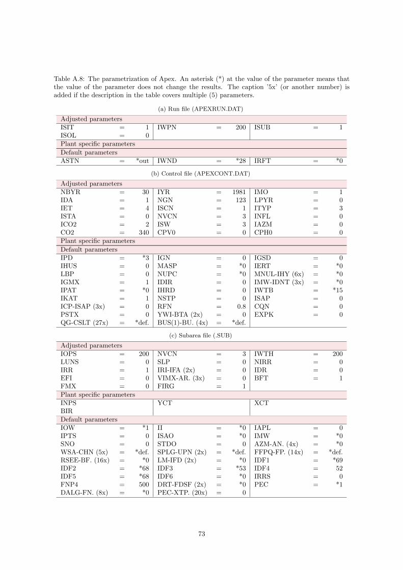
Table A.8: The parametrization of Apex. An asterisk (*) at the value of the parameter means thatthe value of the parameter does not change the results. The caption ’5x’ (or another number) isadded if the description in the table covers multiple (5) parameters.

(a) Run file (APEXRUN.DAT)

Adjusted parametersISIT = 1 IWPN = 200 ISUB = 1ISOL = 0Plant specific parameters

Default parametersASTN = *out IWND = *28 IRFT = *0

(b) Control file (APEXCONT.DAT)

Adjusted parametersNBYR = 30 IYR = 1981 IMO = 1IDA = 1 NGN = 123 LPYR = 0IET = 4 ISCN = 1 ITYP = 3ISTA = 0 NVCN = 3 INFL = 0ICO2 = 2 ISW = 3 IAZM = 0CO2 = 340 CPV0 = 0 CPH0 = 0Plant specific parameters

Default parametersIPD = *3 IGN = 0 IGSD = 0IHUS = 0 MASP = *0 IERT = *0LBP = 0 NUPC = *0 MNUL-IHY (6x) = *0IGMX = 1 IDIR = 0 IMW-IDNT (3x) = *0IPAT = *0 IHRD = 0 IWTB = *15IKAT = 1 NSTP = 0 ISAP = 0ICP-ISAP (3x) = 0 RFN = 0.8 CQN = 0PSTX = 0 YWI-BTA (2x) = 0 EXPK = 0QG-CSLT (27x) = *def. BUS(1)-BU. (4x) = *def.

(c) Subarea file (.SUB)

Adjusted parametersIOPS = 200 NVCN = 3 IWTH = 200LUNS = 0 SLP = 0 NIRR = 0IRR = 1 IRI-IFA (2x) = 0 IDR = 0EFI = 0 VIMX-AR. (3x) = 0 BFT = 1FMX = 0 FIRG = 1Plant specific parametersINPS YCT XCTBIRDefault parametersIOW = *1 II = *0 IAPL = 0IPTS = 0 ISAO = *0 IMW = *0SNO = 0 STDO = 0 AZM-AN. (4x) = *0WSA-CHN (5x) = *def. SPLG-UPN (2x) = *def. FFPQ-FP. (14x) = *def.RSEE-BF. (16x) = *0 LM-IFD (2x) = *0 IDF1 = *69IDF2 = *68 IDF3 = *53 IDF4 = 52IDF5 = *68 IDF6 = *0 IRRS = 0FNP4 = 500 DRT-FDSF (2x) = *0 PEC = *1DALG-FN. (8x) = *0 PEC-XTP. (20x) = 0

73

Table A.8: (continued) The parametrization of Apex. An asterisk (*) at the value of the parametermeans that the value of the parameter does not change the results. The caption ’5x’ (or anothernumber) is added if the description in the table covers multiple (5) parameters.

(d) Operations file (.OPS or .OPC)

Adjusted parametersLUN = 28Plant specific parametersOp. linesDefault parametersIAUI = 500 IAUF = 261 IAMF = 268ISPF = 266 ILQF = 265 IAUL = 267

(e) Site file (.SIT)

Adjusted parametersELEV = 0 RFNX = 0.8Plant specific parametersYLAT XLOGDefault parametersAPM = *1 CO2X-CQ. (2x) = 0 UPR = 1000UNR = 1000 FIR0 = 0 BCHL-BC. (2x) = *0WSA1 = *0

parameter BIR. This parameter sets at which stress fertilization is triggered. As nutrient stress isunfavourable in this study, this parameter is set to 1. There is no maximum amount of fertilizer(FMX). The final parameter that is adjusted is FIRG, which states to which fraction of field capacitythe simulation will irrigate. This is set at 1, meaning that irrigation will return the soil water contentto field capacity as soon as water stress occurs. The rest of the parameters in the subarea file are leftat their default.

The next file is the operation file. While this one is important, most of the operations are plantspecific. The land use number (LUN) is adjusted. The model uses this to determine the curve number.Setting it to 28 corresponds with woods with fair hydrological conditions, which seems appropriatefor all simulations in this study. Only for the grapevines this might not be fully correct, but it ischosen here to keep this a general parameter for simplicity. As the curve number of Apex is alsoused in Aquacrop, inconsistencies between the models do not occur regarding this. The rest of theparameters describe the automatic irrigation type, fertilization type etcetera. These are all left atdefault. For irrigation this is sprinkler type irrigation.

The site file is the last of the run files. In here, the latitude (YLAT) and longitude (XLOG) needto be set again. These depend on the location chosen. The elevation of the land is in all cases setat zero, since no height information is available. The parameter RFNX is the same as the parameterRFN in the control file. The value is therefore also set identical. The rest of the parameters are leftat default.

A.4 Plant implementation

With all the general parameters set-up in the model, the plant parameters should be implementedas well to make a simulation possible. The plant implementation is described in this section in twosteps. First of all, the green-up dates and harvest dates are derived. This is important, as the projectfile of Aquacrop and the operation file of Apex require this data. The second step is to determinethe parameters of the plant file itself. To make a clear separation between the method to derivethe plant parameters and the values of the plant parameters, this second step is divided into threesections. First additional information for Aquacrop is given, followed by additional information forApex. These two sections describe the necessary information to get the plant data. After this, theplant data itself is presented, per plant and per model.

74

Table A.9: The green-up dates and potential heat units for each of the plants. The green-up datesare based on Chapagain and Hoekstra (2004). The potential heat units are retrieved from Apex.

Plant Green-up date Potential heat unitsApple tree (Sh) January 15 2763Apple tree (Ga) January 15 2267Apple tree (Wa) January 15 1675Grapevine April 15 2002Olive tree April 15 3185Oil palm February 15 5966

A.4.1 Green-up and harvest dates

As calculations are done in heat units, harvest takes place a certain amount of accumulated heatunits after sowing or, with woodies, green-up. So to calculate the harvest date, the accumulated heatunits for a plant until harvest, the so-called potential heat units, and the green-up date should beknown. To start with the last one, Chapagain and Hoekstra (2004) provide a database with green-updates for all Faostat plants. An overview of the green-up dates is given in table A.9.

To determine the potential heat units of a plant, one can turn to literature. However, Apex doesnot support the input of potential heat units for plants which are, in the model, categorized as treetypes. This applies to all plants but the grapevine. For tree type plants the model calculates theheat units itself by calculating the average daily heat units (so daily average temperature minus basetemperature of the plant) and multiplying this with the time to maturity (when the plant is full-grown) (Williams et al., 2016). However, attempts to check this calculation method leads to highervalues of the potential heat units for the plants. Perhaps there is some unmentioned correction inthe model.

The potential heat units for this study are calculated by Apex. For this, the general set-up asdescribed in section A.3.2 is entered in the model. For the plant specific parameters, the latitude andlongitude and the corresponding soil number are entered for each location. Irrigation is set to full(BIR = 1). For each of the locations, the climate as described in section A.2.1 is entered, with climateaveraged data. This means that the climate data is adjusted such that in the simulation period of 30years each January first has the same climate, each January second has the same climate etcetera.And finally, the operational lines in the operation (.OPS) file consist of a single sowing line (tillageID number 686) with the corresponding sowing date of the plant, a time to maturity of one year anda sowing density corresponding to the one given in section A.4.3 on page 84. The plant ID number isas described in section A.4.3. An example of the operation file of the apple tree is given in figure A.7.The potential heat units are given in table A.9. For grapevine, potential heat units need to entered.A value of 2002 is chosen, as this leads to a harvest date halfway in October, which seems realistic.

With these potential heat units, the harvest dates can be calculated. This by counting the amountof accumulated heat units every day since green-up according to the heat units equation (equationA.4 or A.5, which are in practice the same for Tupper = 40). When these accumulated heat unitsreach the potential heat units, harvest takes place. An overview of all the harvest dates is given intable A.10. It can occur that the plant cannot be harvested before the end of the year, as is always

Simulation schedule of apple trees

28 500 261 268 266 265 267

1 1 15 686 1 82 1 0.00 0.00 0.00 0.00 200.00 0.00 0.00

Figure A.7: The operation file for Apex to simulate the potential heat units for the apple tree inShandong. The first line can contain comments and is not read by Apex. The second line containsthe general parameter as described in section A.3. The third line contains the operation line with thedate (15 January in simulation year 1), the tillage number (686), a machine number (1, irrelevant),the plant number for the plant file (82), the years to maturity (1) and the planting density (200).

75

Table A.10: The harvest dates for the plants in every year. The year number represents the yearwhere the main part of the plant growth takes place; harvest can take place the following year. Theoil palm cannot be harvested in the last year as it cannot complete its life within the year.

Year Ap

ple

tree

(Sh

)

Ap

ple

tree

(Ga)

Ap

ple

tree

(Wa)

Gra

pev

ine

Oli

vetr

ee

Oil

pal

m

1981 10/06 10/21 09/23 03/18 01/15 01/181982 10/13 10/24 10/15 03/18 02/19 01/181983 10/09 09/23 10/05 11/21 12/18 01/181984 11/03 12/18 12/18 03/18 02/11 01/181985 10/28 12/18 10/16 10/11 12/15 01/181986 10/30 09/23 10/07 10/18 12/18 01/181987 10/27 12/18 09/20 10/03 12/27 01/181988 10/15 10/17 10/08 11/07 01/02 01/181989 10/16 10/08 10/06 10/05 11/29 01/181990 10/16 10/06 09/14 09/28 11/24 01/181991 10/23 10/19 10/02 10/05 01/11 01/181992 10/20 10/17 09/02 11/05 02/06 01/181993 10/27 11/08 12/18 03/18 03/05 01/181994 09/28 09/21 09/14 10/10 12/13 01/181995 10/17 10/04 10/07 10/16 12/11 01/181996 10/25 10/19 10/12 03/07 01/27 01/181997 09/30 12/18 09/25 10/18 12/09 01/181998 10/06 09/28 09/06 10/16 01/10 01/181999 10/06 09/19 12/18 10/08 01/06 01/182000 09/30 09/19 10/11 10/15 01/25 01/182001 10/04 09/22 09/26 10/09 01/07 01/182002 10/03 09/16 10/15 10/25 01/04 01/182003 11/01 09/26 09/09 09/18 12/05 01/182004 10/09 10/17 09/11 10/06 01/17 01/182005 10/09 10/03 09/23 09/25 12/21 01/182006 10/07 10/04 09/18 09/29 11/29 01/182007 10/03 09/02 09/16 10/24 12/28 01/182008 10/18 09/23 10/06 10/28 02/14 01/182009 10/06 09/17 09/15 09/25 12/05 01/182010 10/14 09/15 10/10 10/01 12/20 -

the case for oil palm. In the last year this leads to a problem, as the data only lasts to 31 December.Therefore the oil palm cannot be simulated in the last year.

It is possible that a year is characterized by very low temperatures. This could lead to a situationthat the harvest date is reached after the green-up date of the following year. This is of course notpossible and is avoided by setting the ultimate harvest date 4 weeks (28 days) before the green-update of the following year. By doing this, harvest always takes place before the plant year. It ischosen to set the harvest date 4 weeks before such that the plant has time to recover from its harvest.In reality, a plant will namely not be harvested on one day and starts its new plant year directly theday after. Note that for the oil palm, the harvest date is always limited by this restriction. This iscaused by the (too) high potential heat units.

A.4.2 Additional information Aquacrop

The additional information required to complete the parameter set for Aquacrop consists of a fewsections. First of all, the derivations of the equations for the canopy growth coefficient and the canopy

76

decline coefficient are explained. After this, the method to convert the harvest index of Apex to theone in Aquacrop is given. Following, a method is presented to keep the canopy cover in the winterintact, followed by the equations that describe the parameters for the plant development during theyear. Finally, the rooting depth and the number of plants per hectare are described.

Derivation equation CGC

In Aquacrop, an important parameter for the canopy growth is the canopy growth coefficient (CGC).To calculate the canopy growth coefficient, it is first important to give the general equations of therelation between the canopy cover and the canopy growth coefficient. These are

CC =

{CC o · et·CGC if CC ≤ CC x/2

CC x − 0.25 (CCx)2

CCo· e−t·CGC if CC > CC x/2,

(A.6)

in which CC [m2/m2] is the canopy cover, CC o [m2/m2] and CC x [m2/m2] are plant propertiesthat describe the initial and maximum plant canopy cover, CGC [◦C−1] is the plant specific canopygrowth per heat unit (or GDD) and t [◦C] is the accumulated amount of heat units.

Following the lines of Hofstra (2016), there are two points on the leaf development curve whereit is known which equation is applicable. At the very start of the canopy cover development, whereCC = CC o, it is known that the first equation applies. At the end, where CC = 0.98CC x, thesecond equation is applicable. See figure A.8. If the accumulated heat units corresponding to thesetwo points are called to and tx, the equations can be rewritten in terms of them as

to =1

CGC· ln(

CC o

CC o

)= 0 (A.7)

and

tx = − 1

CGC· ln(

0.08CC o

CC x

). (A.8)

With these two points on the leaf development curve, the distance between these points can becalculated. If the amount of heat units between these two points is called tgrowth, the equation thatapplies is

tgrowth = tx − to, (A.9)

which is the same as

tgrowth = − 1

CGC· ln(

0.08CC o

CC x

)− 0. (A.10)

From this last equation we can derive

CGC = − 1

tgrowth· ln(

0.08CC o

CC x

). (A.11)

So, if the initial canopy cover, the maximum canopy cover and the amount of heat units that it takesto go from the first to the last one are known, the canopy growth coefficient can be calculated.

CC

t

CCo

CCx

CC = CCo · et·CGC

CC = CCx − 0.25 (CCx)2

CCo· e−t·CGC

Figure A.8: The location of the canopy cover growth equations on the leaf development curve.

77

Derivation equation CDC

Similar as the derivation of the canopy growth coefficient, also the canopy decline coefficient (CDC)can be calculated. In the Aquacrop documentation the equation for the canopy decline is given as

CC = CC x ·[1− 0.05

(e

CDCCCx

·t − 1)], (A.12)

wherein CDC [◦C−1] is the canopy decline per heat unit. If the canopy cover at the end of the simu-lation is called CC end and the amount of heat units accumulated between the moment of senescenceand the moment of plant maturity (harvest) is called tdecline, the equation can be rewritten in termsof the canopy decline coefficient to

CDC =CC x

tdecline· ln(

21− 20CC end

CC x

). (A.13)

The canopy decline coefficient can be calculated if the amount of heat units between the start ofsenescence and maturity is known, if the maximum canopy cover is known and if the canopy cover atthe end of the simulation is known.

Harvest index for the foliage only

In Aquacrop only the foliage is simulated, with the remainder of the tree implicitly being present asbiomass that is full-grown and can therefore be left out of the simulation. Since the harvest index isnormally the fraction of the aboveground biomass weight that becomes yield, the harvest index hasto be corrected to become the fraction of the foliage weight only. The relation can be written as

Y = HI st ·Bst = HI fol ·Bfol (A.14)

which, if written in terms of the harvest index for the foliage, is

HI fol = HI st ·Bst

Bfol, (A.15)

in which Y [ton/ha] is the yield, Bst [ton/ha] the standing (aboveground) biomass and Bfol [ton/ha]the weight of the foliage only. Furthermore HI st [−] is the harvest index applicable on the wholestanding biomass and HI fol [−] the harvest index of the foliage only. Given equation A.15, theharvest index of the foliage can easily be calculated if the fraction between the standing biomass andthe foliage biomass is known. In this study, this fraction is derived from literature.

Table A.11: The fraction foliage to total aboveground biomass for different woody plants. As can beseen, most information is available for plants not considered in this study. The foliage weight doesnot include the weight of fruits of the plant, if applicable.

Plant Bfol/Bst Remark SourceApple tree 0.168 4 varieties, max. age 3 years, sick Beers and Hull (1995)Apple tree 0.205 producing trees, 4 temperatures Greer and Wunsche (2003)Banana plant 0.222 different nutrient treatments Lizarazo et al. (2013)Beech tree 0.162 Konopka et al. (2010)Cacao plant 0.160 2 types of water stress Moser et al. (2010)Citrus tree 0.524 very high values Vu and Yelenosky (1988)Oak tree 0.115 Konopka et al. (2010)Oil palm 0.368 producing trees Corley and Tinker (2016)Orange tree 0.258 from literature, range 0.449-0.116 Morgan et al. (2006)Orange tree 0.271 own research Morgan et al. (2006)Pine tree 0.273 Konopka et al. (2010)Pine tree 0.427 4 different water treatments Waghorn et al. (2015)Spruce tree 0.339 Konopka et al. (2010)Average 0.268

78

Table A.11 provides a literature overview of this fraction. As can be seen, the fractions varyconsiderably between different sources, even within one plant species (for example pine trees). Also,not all plants considered in this study are discussed in literature. Therefore a single fraction betweenthe foliage weight and the standing biomass weight is derived for all plants. As the accuracy of tableA.11 is little, the fraction is chosen as 0.25. As a consequence, the harvest index for the foliage willbe 4 times higher than the harvest index for the whole plant. It is important to realize that this is avery rough estimate and the actual fraction will differ per plant and can deviate tremendously fromthis value. However, since the available literature does not allow for a better estimate we have toassume this fraction. Additional (field) research will help to derive a better fraction, possibly plantspecific.

Canopy cover in winter

Aquacrop simulates the plant in this study as if it is a herbaceous plant such as a grain. This meansthat the plant starts growing at green-up and dies at the moment of harvest. The time between theharvest in one year and the green-up in the following year, the agricultural land can be consideredwasteland as no growth takes place. As a result transpiration will become zero during these wintermonths.

To avoid a winter period without transpiration, which is unrealistic for a perennial plant, thegreen-up of a new plant can take place directly after harvest. This by adjusting the green-up date

1985 1986 1987 1988

10

30

50

70

90

Can

opy

cove

r[m

2/m

2]

Without CC in winter

With CC in winter

(a) Canopy cover 1985-1987 in Shandong

1985 1986 1987 1988

1

3

5

7

Tra

nsp

irat

ion

[mm

]

Without CC in winter

With CC in winter

(b) Transpiration 1985-1987 in Shandong

1985 1986 1987 1988

0.1

0.4

0.7

1

Eva

por

atio

n[mm

] Without CC in winter

With CC in winter

(c) Evaporation 1985-1987 in Shandong

Figure A.9: The effect of winter canopy on the evaporation and transpiration. As can be seen,transpiration still occurs in the winter months when the green-up is directly after the harvest.

79

and guaranteeing instant emergence (by setting heat units to emergence on -1, see section A.3.1).The effect of this can be seen in figure A.9. In winter months, the green-up takes place directly afterharvest, leaving the canopy cover intact. However, as a consequence, the plant development will startsomewhere at the end of a certain year, instead of the beginning of the following year. The heat unitsaccumulation in this extended growing period should be added to the amount of heat units to thegrowing phases, such as heat units to flowering and maturity (harvest), to avoid early senescence ofthe plant.

When the heat units are added to each of the growing phases, the resulting canopy cover is theone of figure A.9a. As the canopy development starts earlier, the canopy cover of the winter canopywill stay above the alternative without winter canopy deep into the life of the plant. However, ascan be seen, at some point the two lines of canopy cover will join again and the remaining monthsof a plants life the plant development follows its original path. Because of the early emergence, thetranspiration will be higher and thus the biomass and yield will be slightly higher.

Looking at figure A.9b, it can be seen that transpiration remains very close to the original one.The only significant difference is found in winter months, what was aimed for. It is hard to seein the figure, but in the rest of the year the transpiration is slightly higher than the original. Thetranspiration in the winter months fits quite smoothly between the transpiration at the momentof harvest and the transpiration at the original moment of green-up. In the situation shown here,there is a slight increase of transpiration visible directly after harvest, caused by the change of thetranspiration coefficient Kctr,x. More on this coefficient in the following section.

As can be seen in figure A.9c, the evaporation with the winter canopy deviates from the originalsituation a little. The evaporation tends to stay a little below the original one. This can be explainedby the fact that the canopy cover is higher, and thus relative more transpiration and less evaporationtakes place. This can also be seen with the sum of the two, the evapotranspiration, which is identicalto the original one except for in the winter months. The evapotranspiration is not shown here.

Because the winter canopy allows for a more realistic transpiration behaviour, it is implementedin the model.

Annual life cycle of a plant

As shown before, and shown again in figure A.10a, the canopy covers develops over a year. It growsfrom an initial canopy cover to a maximum canopy cover, where after it decreases again to its canopycover at maturity. For each of the plants, these initial, maximum and final canopy cover have to bedetermined. In addition, the heat units from initial to maximum canopy cover, the number of heatunits that it stays on its maximum and the number of heat units that it takes to go from maximumto final canopy cover have to be found.

To link the reference evapotranspiration with the actual evapotranspiration, a plant factor withthe symbol k is generally used. This plant factor changes over the year, due to the fact that the plantdevelops over the year and thus the amount of transpiration that takes place from a plant changes.The change of this plant factor can be seen in figure A.10b. As can be seen, the plant factor is alsocharacterized by an initial factor, a maximum factor and a final factor. Chapagain and Hoekstra(2004) give an overview of these plant factors for every Faostat plant (which include the apple tree,the grapevine, the olive tree and the oil palm). Also the length between the different phases is givenby them.

With this information about the canopy cover and the plant factor, it is a small step to see thatthe data concerned with the plant factor can also be used to determine the different canopy covers

time0

1

CC

CCx

CCo

CCend

tx

tsen

tmat

(a) Canopy cover

time0

k

kx

ko

kend

Lo Lg Lx Ld

(b) Plant factor

Figure A.10: The canopy cover on one hand and the comparable plant factor on the other hand.

80

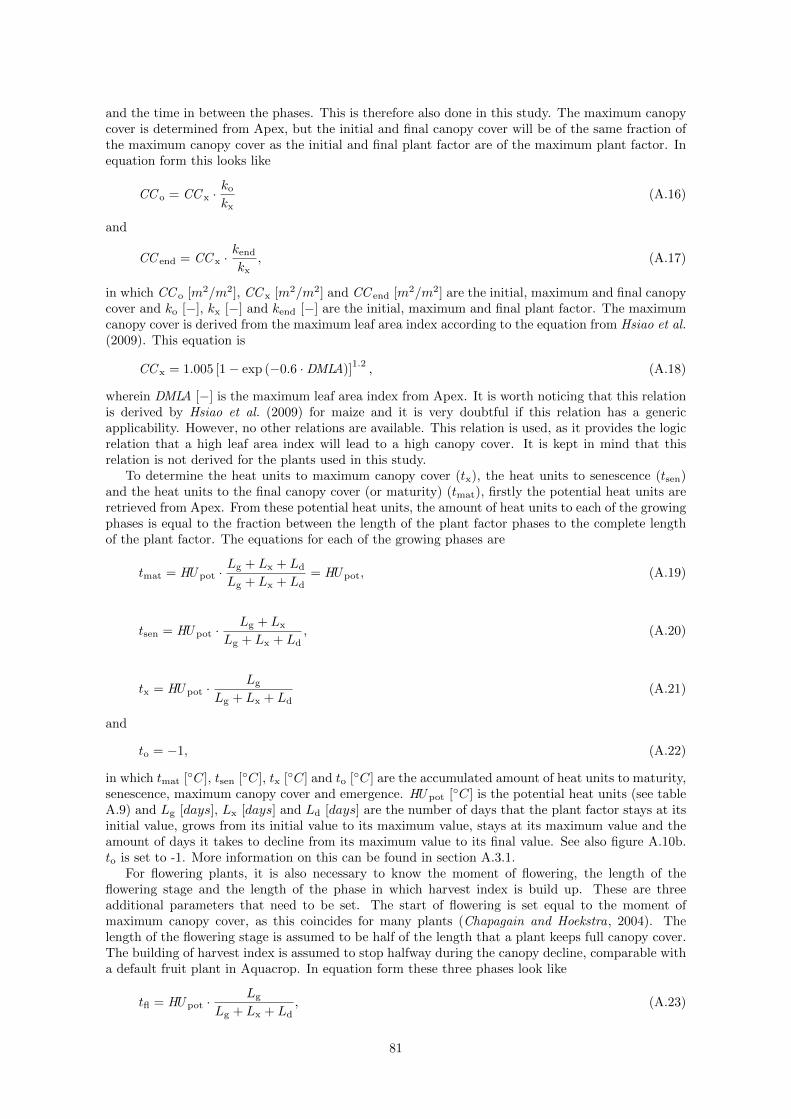
and the time in between the phases. This is therefore also done in this study. The maximum canopycover is determined from Apex, but the initial and final canopy cover will be of the same fraction ofthe maximum canopy cover as the initial and final plant factor are of the maximum plant factor. Inequation form this looks like

CC o = CC x ·ko

kx(A.16)

and

CC end = CC x ·kend

kx, (A.17)

in which CC o [m2/m2], CC x [m2/m2] and CC end [m2/m2] are the initial, maximum and final canopycover and ko [−], kx [−] and kend [−] are the initial, maximum and final plant factor. The maximumcanopy cover is derived from the maximum leaf area index according to the equation from Hsiao et al.(2009). This equation is

CC x = 1.005 [1− exp (−0.6 ·DMLA)]1.2, (A.18)

wherein DMLA [−] is the maximum leaf area index from Apex. It is worth noticing that this relationis derived by Hsiao et al. (2009) for maize and it is very doubtful if this relation has a genericapplicability. However, no other relations are available. This relation is used, as it provides the logicrelation that a high leaf area index will lead to a high canopy cover. It is kept in mind that thisrelation is not derived for the plants used in this study.

To determine the heat units to maximum canopy cover (tx), the heat units to senescence (tsen)and the heat units to the final canopy cover (or maturity) (tmat), firstly the potential heat units areretrieved from Apex. From these potential heat units, the amount of heat units to each of the growingphases is equal to the fraction between the length of the plant factor phases to the complete lengthof the plant factor. The equations for each of the growing phases are

tmat = HU pot ·Lg + Lx + Ld

Lg + Lx + Ld= HU pot, (A.19)

tsen = HU pot ·Lg + Lx

Lg + Lx + Ld, (A.20)

tx = HU pot ·Lg

Lg + Lx + Ld(A.21)

and

to = −1, (A.22)

in which tmat [◦C], tsen [◦C], tx [◦C] and to [◦C] are the accumulated amount of heat units to maturity,senescence, maximum canopy cover and emergence. HU pot [◦C] is the potential heat units (see tableA.9) and Lg [days], Lx [days] and Ld [days] are the number of days that the plant factor stays at itsinitial value, grows from its initial value to its maximum value, stays at its maximum value and theamount of days it takes to decline from its maximum value to its final value. See also figure A.10b.to is set to -1. More information on this can be found in section A.3.1.

For flowering plants, it is also necessary to know the moment of flowering, the length of theflowering stage and the length of the phase in which harvest index is build up. These are threeadditional parameters that need to be set. The start of flowering is set equal to the moment ofmaximum canopy cover, as this coincides for many plants (Chapagain and Hoekstra, 2004). Thelength of the flowering stage is assumed to be half of the length that a plant keeps full canopy cover.The building of harvest index is assumed to stop halfway during the canopy decline, comparable witha default fruit plant in Aquacrop. In equation form these three phases look like

tfl = HU pot ·Lg

Lg + Lx + Ld, (A.23)

81

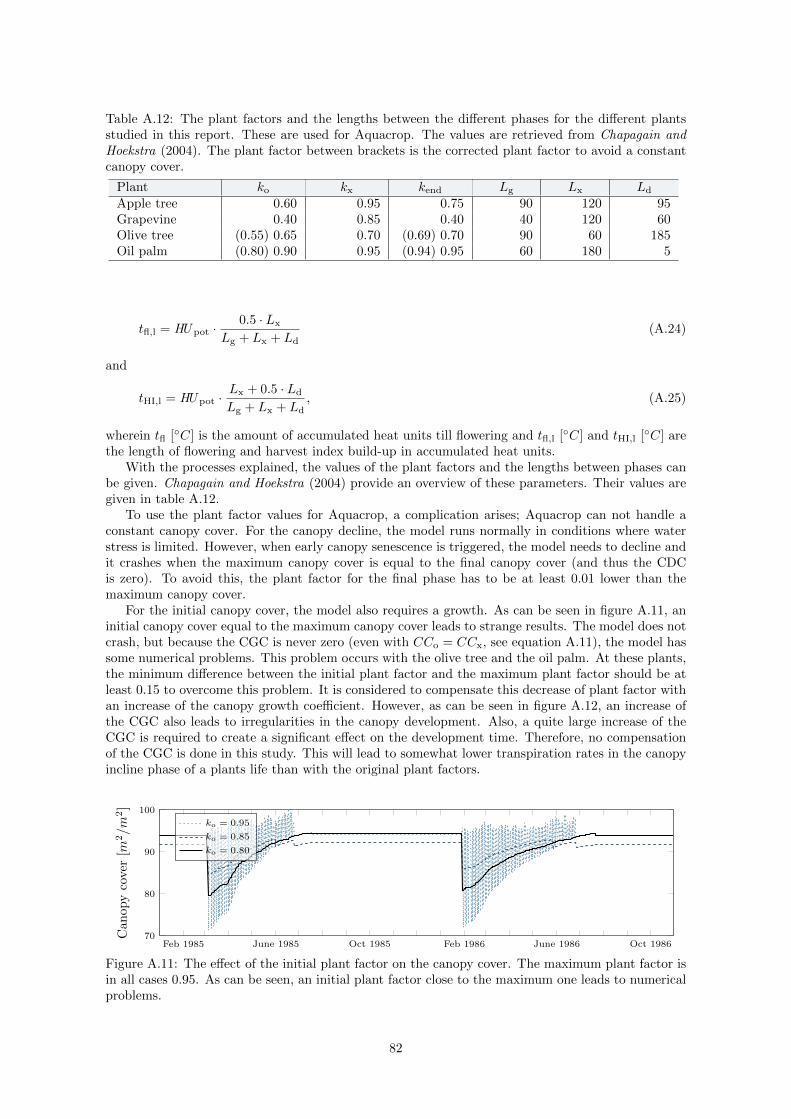
Table A.12: The plant factors and the lengths between the different phases for the different plantsstudied in this report. These are used for Aquacrop. The values are retrieved from Chapagain andHoekstra (2004). The plant factor between brackets is the corrected plant factor to avoid a constantcanopy cover.

Plant ko kx kend Lg Lx Ld

Apple tree 0.60 0.95 0.75 90 120 95Grapevine 0.40 0.85 0.40 40 120 60Olive tree (0.55) 0.65 0.70 (0.69) 0.70 90 60 185Oil palm (0.80) 0.90 0.95 (0.94) 0.95 60 180 5

tfl,l = HU pot ·0.5 · Lx

Lg + Lx + Ld(A.24)

and

tHI,l = HU pot ·Lx + 0.5 · Ld

Lg + Lx + Ld, (A.25)

wherein tfl [◦C] is the amount of accumulated heat units till flowering and tfl,l [◦C] and tHI,l [◦C] arethe length of flowering and harvest index build-up in accumulated heat units.

With the processes explained, the values of the plant factors and the lengths between phases canbe given. Chapagain and Hoekstra (2004) provide an overview of these parameters. Their values aregiven in table A.12.

To use the plant factor values for Aquacrop, a complication arises; Aquacrop can not handle aconstant canopy cover. For the canopy decline, the model runs normally in conditions where waterstress is limited. However, when early canopy senescence is triggered, the model needs to decline andit crashes when the maximum canopy cover is equal to the final canopy cover (and thus the CDCis zero). To avoid this, the plant factor for the final phase has to be at least 0.01 lower than themaximum canopy cover.

For the initial canopy cover, the model also requires a growth. As can be seen in figure A.11, aninitial canopy cover equal to the maximum canopy cover leads to strange results. The model does notcrash, but because the CGC is never zero (even with CCo = CCx, see equation A.11), the model hassome numerical problems. This problem occurs with the olive tree and the oil palm. At these plants,the minimum difference between the initial plant factor and the maximum plant factor should be atleast 0.15 to overcome this problem. It is considered to compensate this decrease of plant factor withan increase of the canopy growth coefficient. However, as can be seen in figure A.12, an increase ofthe CGC also leads to irregularities in the canopy development. Also, a quite large increase of theCGC is required to create a significant effect on the development time. Therefore, no compensationof the CGC is done in this study. This will lead to somewhat lower transpiration rates in the canopyincline phase of a plants life than with the original plant factors.

Feb 1985 June 1985 Oct 1985 Feb 1986 June 1986 Oct 198670

80

90

100

Can

opycover[m

2/m

2]

ko = 0.95

ko = 0.85

ko = 0.80

Figure A.11: The effect of the initial plant factor on the canopy cover. The maximum plant factor isin all cases 0.95. As can be seen, an initial plant factor close to the maximum one leads to numericalproblems.

82

Feb 1985 June 1985 Oct 1985 Feb 1986 June 1986 Oct 198670

80

90

100Can

opycover[m

2/m

2]

base

CGC · 1.15CGC · 2.00CGC · 4.00

Figure A.12: The effect of a higher canopy growth coefficient on the canopy cover. As can be seen,a higher CGC leads to some inconsistent development patterns of the canopy cover.

Feb 1982 May 1982 Aug 1982 Nov 19820

0.3

0.6

0.9

1.2

Rootingdepth

[m] Variable rooting depth

Constant rooting depth

Figure A.13: A comparison between a variable rooting depth (minimum rooting depth different thanmaximum rooting depth) and a constant rooting depth (minimum rooting depth equal to maximumrooting depth) for Shandong in 1982.

Rooting depth

In Aquacrop, two parameters are the minimum and maximum rooting depth. These two parametersdescribe the initial and final rooting depth. Two additional parameters describe the time, in this casein heat units, it takes to go from the minimum to the maximum rooting depth and the shape of theroot development.

For the simulations in this study, the plant is considered full grown. This means that not only thebiomass is full grown, but also the roots should be fully developed from the start of the simulation.To reach this, the minimum rooting depth is set equal to the maximum rooting depth. Aquacroprecognizes this as a constant rooting depth equal to the maximum rooting depth. This can be seenin figure A.13.

To harmonize the values between Aquacrop and Apex, the maximum rooting depth is chosen fromApex. However, in Apex the maximum rooting depth is the minimum of the depth of the soil profileand the maximum rooting depth, with the reason that the roots of the plant can never be deeper thanthe soil profile itself. In Aquacrop, such a constrain is not available, but because of harmonizationreasons the rooting depth in Aquacrop is also maximum the soil profile depth.

Plants per hectare

The amount of plants per hectare is an important parameter in Aquacrop. Together with the initialcover of a seedling it sets the initial canopy cover. From equation A.16 it is known how the initialcanopy cover can be calculated. From table A.7a it is furthermore known that the soil cover per plantis set equal to 200 cm2. To calculate the number of plants per hectare, the equation that can be usedis

pph =CC o · 108

200, (A.26)

wherein pph [ha−1] are the number of plants per hectare. The factor 108 comes from the fact thatthe soil cover per plant of 200 cm2 should be calculated from square centimetre to hectare.

83

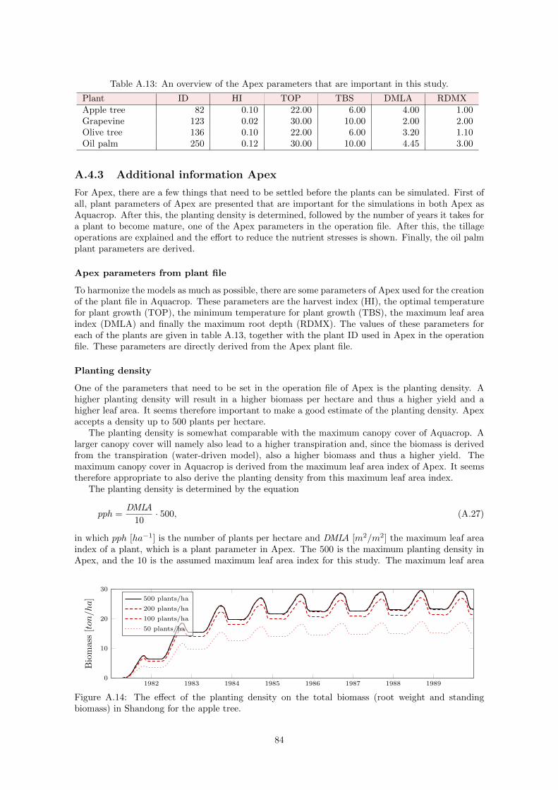
Table A.13: An overview of the Apex parameters that are important in this study.

Plant ID HI TOP TBS DMLA RDMXApple tree 82 0.10 22.00 6.00 4.00 1.00Grapevine 123 0.02 30.00 10.00 2.00 2.00Olive tree 136 0.10 22.00 6.00 3.20 1.10Oil palm 250 0.12 30.00 10.00 4.45 3.00

A.4.3 Additional information Apex

For Apex, there are a few things that need to be settled before the plants can be simulated. First ofall, plant parameters of Apex are presented that are important for the simulations in both Apex asAquacrop. After this, the planting density is determined, followed by the number of years it takes fora plant to become mature, one of the Apex parameters in the operation file. After this, the tillageoperations are explained and the effort to reduce the nutrient stresses is shown. Finally, the oil palmplant parameters are derived.

Apex parameters from plant file

To harmonize the models as much as possible, there are some parameters of Apex used for the creationof the plant file in Aquacrop. These parameters are the harvest index (HI), the optimal temperaturefor plant growth (TOP), the minimum temperature for plant growth (TBS), the maximum leaf areaindex (DMLA) and finally the maximum root depth (RDMX). The values of these parameters foreach of the plants are given in table A.13, together with the plant ID used in Apex in the operationfile. These parameters are directly derived from the Apex plant file.

Planting density

One of the parameters that need to be set in the operation file of Apex is the planting density. Ahigher planting density will result in a higher biomass per hectare and thus a higher yield and ahigher leaf area. It seems therefore important to make a good estimate of the planting density. Apexaccepts a density up to 500 plants per hectare.

The planting density is somewhat comparable with the maximum canopy cover of Aquacrop. Alarger canopy cover will namely also lead to a higher transpiration and, since the biomass is derivedfrom the transpiration (water-driven model), also a higher biomass and thus a higher yield. Themaximum canopy cover in Aquacrop is derived from the maximum leaf area index of Apex. It seemstherefore appropriate to also derive the planting density from this maximum leaf area index.

The planting density is determined by the equation

pph =DMLA

10· 500, (A.27)

in which pph [ha−1] is the number of plants per hectare and DMLA [m2/m2] the maximum leaf areaindex of a plant, which is a plant parameter in Apex. The 500 is the maximum planting density inApex, and the 10 is the assumed maximum leaf area index for this study. The maximum leaf area

1982 1983 1984 1985 1986 1987 1988 19890

10

20

30

Biomass[ton

/ha] 500 plants/ha

200 plants/ha

100 plants/ha

50 plants/ha

Figure A.14: The effect of the planting density on the total biomass (root weight and standingbiomass) in Shandong for the apple tree.

84

index of 10 is based on the database of leaf area indices of Iio and Ito (2014), in which a leaf areaindex higher than 10 occurs only in less than five percent of the cases. This equation thus takes theleaf area index relative to the maximum and uses this ratio also for the planting density.

This relation seems like a rough estimate, and it is. However, as can be seen in figure A.14, themodel is not as sensitive to different planting density as one would expect. It was expected that aplanting density half the size would also half the biomass production (and thus the yield), but this isclearly not the case. Therefore it is chosen to use this rough theoretical approximation of the plantingdensity in the operation files.

Years to maturity

Next to the planting density, a parameter that states the number of years it takes a tree to becomemature (or full-grown) is present in the operation file. This parameter needs to be set for every plantin this study, except the grapevine as this is not a tree. The effect of the time to maturity can be seenin figure A.15. The time to maturity has a strong effect on the biomass (and thus the yield), as themodel keeps accumulating biomass for a tree. As the leaf area index is bounded to a maximum, theLAI stabilizes after the years to maturity is reached and therefore the effect of the time to maturityon the evaporation and transpiration is limited.

In Aquacrop, a mature plant has reached the end of its life and dies, but in Apex the maturity ofthe tree is not well defined. A tree is considered mature when the heat unit index of the plant hasreached one (potential heat units is reached). Since the leaf area index develops with the heat unitindex, the LAI is also at its full when the tree is mature. What the role of biomass is in this remainsunclear, as this is not discussed in the documentation of the model.

In literature there is no clear overview of the time it takes for a plant to become fully grown andcan thus be considered mature in Apex. An estimate is therefore made for this study, although theparameter is important for the yield (see figure A.15). For this study, it is chosen to set the time tomaturity for all plants on five years. This seems reasonable, as this still allows for a clear developmentphase of the plant, while in most cases also reaching an equilibrium for the biomass within the 30years of simulation, which is convenient for the analysis of the results. In reality, the time wouldprobably be somewhat higher (see for example Flore et al. (1984)).

1982 1986 1990 1994 1998 20020

55

110

165

220

Bio

mas

s[ton/ha] 10 years to maturity

5 years to maturity

2 years to maturity

1 years to maturity

(a) Total biomass 1981-2004 in Shandong

1982 1986 1990 1994 1998 20020

1

2

3

4

LA

I[m

2/m

2]

(b) Leaf area index 1981-2004 in Shandong

Figure A.15: The effect of the time to maturity on the biomass and the leaf area index. The biomass(and thus the yield) rises when the years to maturity increase.

85

Tillage operations

In the operation file of Apex, the tillage operation ID numbers need to be set. For sowing operations,tillage number 686 is used, which is sowing by hand. For the harvest operations, harvest by hand isapplied, which is operation 683. For the application of nutrients (see next section), tillage operation684 is used, which is fertilizer by hand.

Reducing nutrient stresses

There are no nutrient stresses being simulated in Aquacrop. To avoid these stresses also in Apex,automatic fertilizer is set (see section A.3.2). This will start fertilizing as soon as stresses are noticed.In addition to this, some precautionary fertilization is applied every year. On the date that sowingtook place, the maximum amount of fertilizer is applied in the operation file. This amount, 500kilogram per hectare, is applied with tillage number 684, which is fertilization by hand. The type offertilizer applied is number 53, which is nitrogen.

Implementing oil palm

The apple tree, the grapevine and the olive tree are all standard in Apex. Unfortunately, oil palm isnot and it is therefore necessary to add this plant to the plant file of Apex. The parameters, all 64,need to be estimated. A lot of these parameters, however, will be irrelevant as they are applicable toprocesses that are not considered in this study, such as costs.

To develop the oil palm effectively, the coconut palm is used as a basis. Most of the parametersof this plant will be used for the oil palm as well. Based on Legros et al. (2009), there are fourparameters adjusted. These are the harvest index (HI), the maximum leaf area index (DMLA), themaximum height (HMX) and the maximum root depth (RDMX) of the plant. Legros et al. (2009)present a harvest index for the oil palm of 0.48. This seems high, but this is the dry fruit biomassproduction in relation with the dry aboveground biomass production. In other words, this is the

Table A.14: The parameters of the newly created oil palm in Apex, based on the coconut palm andthe apple tree, both already in the model. The asterisk (*) represent a user definable number orname.

Oil palm# = *250 NAME = *OILP WA = 24.00HI = 0.12 TOP = 30.00 TBS = 10.00DMLA = 4.45 DLAI = 0.90 DLAP1 = 15.05DLAP2 = 50.99 RLAD = 1.00 RBMD = 1.00ALT = 3.00 GSI = 0.007 CAF = 0.85SDW = 100.00 HMX = 9.00 RDMX = 3.00WAC2 = 660.30 CNY = 0.0015 CPY = 0.0003CKY = 0.00 WSYF = 0.05 PST = 0.60COSD = 0.00 PRYG = 0.00 PRYF = 0.00WCY = 0.50 BN1 = 0.006 BN2 = 0.002BN3 = 0.0015 BP1 = 0.0007 BP2 = 0.0004BP3 = 0.0003 BK1 = 3.39 BK2 = 3.39BK3 = 3.39 BW1 = 8.00 BW2 = 5.10BW3 = 15.99 IDC = 8.00 FRST1 = 0.50FRST2 = 4.75 WAVP = 0.40 VPTH = 0.20VPD2 = 20.00 RWPC1 = 0.40 RWPC2 = 0.20GMHU = 0.00 PPLP1 = 120.88 PPLP2 = 20.13STX1 = 0.10 STX2 = 0.00 BLG1 = 0.05BLG2 = 0.00 WUB = 0.30 FTO = 0.00FLT = 0.00 CCEM = 0.00 IPDU = 0.00TRE1 = 0.00 TRE2 = 0.00 LAYR = 0.00WDRM = 0.00 EXTC = 0.00 GPAL = 0.00FNAME = *OILP

86

harvest index for Aquacrop, as it only considers the build up of biomass within the year. Assumingthe harvest index relation between the yearly biomass build and the total biomass build of a factorfour (see section A.4.2), the harvest index for Apex becomes 0.12. The leaf area index they observedhad an average of 4.45. The average stem height they observed was about 9 meters. The maximumroot depth is set to 3 meters, as they observed most roots to be present within these 3 meters.

Only changing these four parameters will not lead to a functioning tree in Apex. To allow for plantgrowth, the plant population parameters PPLP1 and PPLP2 should be changed. The parametersbelonging to the coconut tree are such that a plant will not grow. For these two parameters, theparameters for the apple tree are used. Furthermore, the partitioning of the total biomass into rootweight and aboveground biomass need to be adjusted, as the coconut tree parameters are such thatover 90 percent of the total biomass is allocated to the roots, which is unrealistic. The parametersconcerned with this, RWPC1 and RWPC2, are also taken from the apple tree. An overview of allparameters of the created oil palm file is found in table A.14.

To simulate oil palms in Apex, there is one important step remaining. In this study, oil palmsare simulated in Malaysia, at a latitude of 2.25 decimal degrees. Unfortunately, Apex gives strangeresults at such low latitudes, as the model simulates dormancy in the period where the day length iswithin an hour of the shortest day length. In other words, when the shortest day length is six hours,the model simulates dormancy every day that the day length is lower than seven hours. Around theequator, however, this condition leads to a situation where there is always dormancy, as the day lengthis always within the hour of the minimum day length. Therefore, the used latitude for oil palm is setto 45.00 decimal degrees. Another option would be to adjust the parameters file (PARMS.DAT) forthe oil palm such that the dormancy criterion of an hour is reduced to any fraction of this. However,as this leads to strange model behaviour and because of the warnings given with the parameters file,the latitude is changed instead.

A.4.4 Plant data

Based on the information given in section A.4.2 for Aquacrop and section A.4.3 for Apex, all of theplant or location specific parameters of the models can be filled in. In table A.15 an overview on howto determine the parameters in each of the files.

With the information on how to get the plant specific parameters, the files to run the simulationscan be created. In table A.16 an overview is given of the values for all parameters at all locations.Note that the dates and the operation lines are left out of the table. An example of a project file ofAquacrop is shown in figure A.16a. An example of a operation file of Apex is given in figure A.16b.

In Aquacrop, the green-up date (first day of cropping period in figure A.16a) is the date given intable A.9. This is only for the first year; the following years the first day of the cropping period is theday following the harvest date. This to keep canopy intact throughout the winter (see section A.4.2).The harvest date (last day of cropping period) is the date given in table A.10. The first day of thesimulation is always the same as the first day of the cropping period, except for the first year, whenit is equal to the first of January. The last day of the simulation is one day before harvest. Whensetting it equal to the harvest date, the model will start the simulation of the new season a day later,causing a day with no canopy cover and thus no transpiration. To avoid this, the harvest date is setone day early. In the last year, the last day of the simulation period is equal to the 31st of December.

For Apex, the first operation is always the sowing date of the plant. This should be entered withits corresponding time to maturity, plant number and density. On the same day of sowing, fertilizerapplication takes place to reduce nutrient stresses. The maximum amount of fertilizer is applied,in combination with the correct plant number, tillage number and fertilizer number. Every yearthis operation is repeated to prevent nutrient stress. On top of these sowing operation and fertilizerapplications, harvest takes place on the dates given in table A.10. Also for harvest operations, thecorrect plant number, tillage number and time to maturity should be entered correctly.

87

Table A.15: An overview of all the plant or location specific parameters and the way they can bedetermined. The motivation for the method to determine them is explained in sections A.4.2 andA.4.3.

(a) Aquacrop

Aquacrop parametersSymbol Parameter DerivationTbase Base temperature Apex paramtr. TBS (table A.13)GDupper Min. GDD for biomass Apex paramtr. TOP-TBS, < 20 ◦C (table A.13)tmat Length cycle in GDD Potential heat units (table A.9)KcTr,x Crop coefficient Maximum plant factor (table A.12)Zo Min. eff. root depth Min. Apex paramtr. RDMX (table A.13) and soil

profile depthZx Max. eff. root depth Min. Apex paramtr. RDMX (table A.13) and soil

profile depthpph Plants per hectare Derived from CC o (equation A.26)CCx Max. CC Derived from Apex paramtr. DMLA (eq. A.18)HIo Reference HI Derived from Apex paramtr. HI (equation A.15)tsen GDD to senescence Derived from plant factor (equation A.20)tmat GDD to maturity Potential heat units (equation A.19, table A.9)tfl GDD to flowering Derived from plant factor (equation A.23)tfl,l Length flow. stage GDD Derived from plant factor (equation A.24)CGC CGC in GDD Derived from CC o and CC x (equation A.11)CDC CDC in GDD Derived from CC end and CC x (equation A.13)thi,l Building up HI in GDD Derived from plant factor (equation A.25)kex Soil evap. coeff. Maximum plant factor (table A.12)Aquacrop remainingSymbol Parameter Derivation− Dates simulation & plant See text in this section

(b) Apex

Apex parametersSymbol Parameter DerivationINPS Soil number See tables A.4 and A.6YCT Latitude See appendix C, table C.1. Oil palm 45.00XCT Longitude See appendix C, table C.1BIR Irrigation fraction 1 if irrigated simulation, 0 if notYLAT Latitude See appendix C, table C.1. Oil palm 45.00XLOG Longitude See appendix C, table C.1Apex remainingSymbol Parameter Derivation− Operation lines See text in this section

88

Table A.16: An overview of the parameter values for each of the locations for the first year. In otheryears the heat units to certain growth stages in Aquacrop differs because of the winter canopy.

Symbol Ap

ple

tree

(Sh

)

Ap

ple

tree

(Ga)

Ap

ple

tree

(Wa)

Gra

pev

ine

Oli

vetr

ee

Oil

palm

Aquacrop parametersTbase 6.0 6.0 6.0 10.0 6.0 10.0GDupper 16.0 16.0 16.0 20.0 16.0 20.0tmat 2763 2267 1675 2002 3185 5966KcTr,x 0.95 0.95 0.95 0.85 0.70 0.95Zo 1.00 1.00 1.00 1.00 1.00 1.00Zx 1.00 1.00 1.00 1.00 1.00 1.00pph 283141 283141 283141 153817 326422 388241CC x 0.90 0.90 0.90 0.65 0.83 0.92HI o 40 40 40 8 40 48tsen 1902 1561 1153 1456 1426 5844tmat 2763 2267 1675 2002 3185 5966tfl 815 669 494 364 856 1461tfl,l 544 446 330 546 285 2192CGC 0.003661 0.004463 0.006040 0.009010 0.003234 0.001846CDC 0.001720 0.002096 0.002837 0.002933 0.000119 0.001447thi,l 1517 1245 920 1365 1450 4444kex 0.95 0.95 0.95 0.85 0.70 0.95Apex parametersINPS 22455 186186 22440 210126 18516 207110YCT 35.56 46.45 46.97 39.31 36.90 45.00XCT 119.16 28.65 -120.76 -2.81 -5.21 103.13BIR 1 or 0 1 or 0 1 or 0 1 or 0 1 or 0 1 or 0YLAT 35.56 46.45 46.97 39.31 36.90 45.00XLOG 119.16 28.65 -120.76 -2.81 -5.21 103.13

89

4.0 : AquaCrop Version (June 2012)

29221 : First day of simulation period - 22 March 1981

29498 : Last day of simulation period - 24 July 1981

29235 : First day of cropping period - 22 March 1981

29499 : Last day of cropping period - 24 July 1981

4 : Evaporation decline factor for stage II

0.95 : Ke(x) Soil evaporation coefficient for fully wet and non-shaded soil...

5 : Threshold for green CC below which HI can no longer increase (% cover)

70 : Starting depth of root zone expansion curve (% of Zmin)

5.00 : Maximum allowable root zone expansion (fixed at 5 cm/day)

-6 : Shape factor for effect water stress on root zone expansion

20 : Required soil water content in top soil for germination (% TAW)

1.0 : Adjustment factor for FAO-adjustment soil water depletion (p) by ETo

3 : Number of days after which deficient aeration is fully effective

1.00 : Exponent of senescence factor adjusting drop in photosynthetic activ...

12 : Decrease of p(sen) once early canopy senescence is triggered (% of p...

0 : Thresholds for water stress for stomatal closure are NOT affected by...

30 : Depth [cm] of soil profile affected by water extraction by soil evap...

0.30 : Considered depth (m) of soil profile for calculation of mean soil wa...

0 : CN is adjusted to Antecedent Moisture Class

20 : salt diffusion factor (capacity for salt diffusion in micro pores) [%]

100 : salt solubility [g/liter]

16 : shape factor for effect of soil water content gradient on capillary ...

12.0 : Default minimum temperature ($ ^\circ $C) if no temperature file is ...

28.0 : Default maximum temperature ($ ^\circ $C) if no temperature file is ...

1 : Default method for the calculation of growing degree days

-- 1. Climate (CLI) file

climatedata.CLI

C:\Zero\AquaCrop\Model\AquaCrop_Shandong\DATA\

1.1 Temperature (TMP) file

climatedata.TMP


1.2 Reference ET (ETo) file

climatedata.ETo


1.3 Rain (PLU) file

climatedata.PLU


1.4 Atmospheric CO2 (CO2) file

climatedata.CO2


-- 2. Crop (CRO) file

Shandong_1.CRO


-- 3. Irrigation (IRR) file

Inet.IRR


-- 4. Management (MAN) file

(None)

(None)

-- 5. Soil profile (SOL) file

SOL_224_55.SOL


-- 6. Groundwater (GWT) file

......

(a) Example project file of Aquacrop for the apple tree in Shandong

Figure A.16: Example of the project file of Aquacrop and the operation file of Apex for the appletree in Shandong. Only the first 55 lines are shown.

90

Simulation schedule of apple trees

28 500 261 268 266 265 267

1 1 15 686 1 82 5 0.00 0.00 0.00 0.00 200.00 0.00 0.00

1 1 15 684 1 82 53 500.00 0.00 0.00 0.00 0.00 0.00 0.00

1 10 6 683 1 82 5 0.00 0.00 0.00 0.00 0.00 0.00 0.00

2 1 15 684 1 82 53 500.00 0.00 0.00 0.00 0.00 0.00 0.00

2 10 13 683 1 82 5 0.00 0.00 0.00 0.00 0.00 0.00 0.00

3 1 15 684 1 82 53 500.00 0.00 0.00 0.00 0.00 0.00 0.00

3 10 9 683 1 82 5 0.00 0.00 0.00 0.00 0.00 0.00 0.00

4 1 15 684 1 82 53 500.00 0.00 0.00 0.00 0.00 0.00 0.00

4 11 3 683 1 82 5 0.00 0.00 0.00 0.00 0.00 0.00 0.00

5 1 15 684 1 82 53 500.00 0.00 0.00 0.00 0.00 0.00 0.00

5 10 28 683 1 82 5 0.00 0.00 0.00 0.00 0.00 0.00 0.00

6 1 15 684 1 82 53 500.00 0.00 0.00 0.00 0.00 0.00 0.00

6 10 30 683 1 82 5 0.00 0.00 0.00 0.00 0.00 0.00 0.00

7 1 15 684 1 82 53 500.00 0.00 0.00 0.00 0.00 0.00 0.00

7 10 27 683 1 82 5 0.00 0.00 0.00 0.00 0.00 0.00 0.00

8 1 15 684 1 82 53 500.00 0.00 0.00 0.00 0.00 0.00 0.00

8 10 15 683 1 82 5 0.00 0.00 0.00 0.00 0.00 0.00 0.00

9 1 15 684 1 82 53 500.00 0.00 0.00 0.00 0.00 0.00 0.00

9 10 16 683 1 82 5 0.00 0.00 0.00 0.00 0.00 0.00 0.00

10 1 15 684 1 82 53 500.00 0.00 0.00 0.00 0.00 0.00 0.00

10 10 16 683 1 82 5 0.00 0.00 0.00 0.00 0.00 0.00 0.00

11 1 15 684 1 82 53 500.00 0.00 0.00 0.00 0.00 0.00 0.00

11 10 23 683 1 82 5 0.00 0.00 0.00 0.00 0.00 0.00 0.00

12 1 15 684 1 82 53 500.00 0.00 0.00 0.00 0.00 0.00 0.00

12 10 20 683 1 82 5 0.00 0.00 0.00 0.00 0.00 0.00 0.00

13 1 15 684 1 82 53 500.00 0.00 0.00 0.00 0.00 0.00 0.00

13 10 27 683 1 82 5 0.00 0.00 0.00 0.00 0.00 0.00 0.00

14 1 15 684 1 82 53 500.00 0.00 0.00 0.00 0.00 0.00 0.00

14 9 28 683 1 82 5 0.00 0.00 0.00 0.00 0.00 0.00 0.00

15 1 15 684 1 82 53 500.00 0.00 0.00 0.00 0.00 0.00 0.00

15 10 17 683 1 82 5 0.00 0.00 0.00 0.00 0.00 0.00 0.00

16 1 15 684 1 82 53 500.00 0.00 0.00 0.00 0.00 0.00 0.00

16 10 25 683 1 82 5 0.00 0.00 0.00 0.00 0.00 0.00 0.00

17 1 15 684 1 82 53 500.00 0.00 0.00 0.00 0.00 0.00 0.00

17 9 30 683 1 82 5 0.00 0.00 0.00 0.00 0.00 0.00 0.00

18 1 15 684 1 82 53 500.00 0.00 0.00 0.00 0.00 0.00 0.00

18 10 6 683 1 82 5 0.00 0.00 0.00 0.00 0.00 0.00 0.00

19 1 15 684 1 82 53 500.00 0.00 0.00 0.00 0.00 0.00 0.00

19 10 6 683 1 82 5 0.00 0.00 0.00 0.00 0.00 0.00 0.00

20 1 15 684 1 82 53 500.00 0.00 0.00 0.00 0.00 0.00 0.00

20 9 30 683 1 82 5 0.00 0.00 0.00 0.00 0.00 0.00 0.00

21 1 15 684 1 82 53 500.00 0.00 0.00 0.00 0.00 0.00 0.00

21 10 4 683 1 82 5 0.00 0.00 0.00 0.00 0.00 0.00 0.00

22 1 15 684 1 82 53 500.00 0.00 0.00 0.00 0.00 0.00 0.00

22 10 3 683 1 82 5 0.00 0.00 0.00 0.00 0.00 0.00 0.00

23 1 15 684 1 82 53 500.00 0.00 0.00 0.00 0.00 0.00 0.00

23 11 1 683 1 82 5 0.00 0.00 0.00 0.00 0.00 0.00 0.00

24 1 15 684 1 82 53 500.00 0.00 0.00 0.00 0.00 0.00 0.00

24 10 9 683 1 82 5 0.00 0.00 0.00 0.00 0.00 0.00 0.00

25 1 15 684 1 82 53 500.00 0.00 0.00 0.00 0.00 0.00 0.00

25 10 9 683 1 82 5 0.00 0.00 0.00 0.00 0.00 0.00 0.00

26 1 15 684 1 82 53 500.00 0.00 0.00 0.00 0.00 0.00 0.00

26 10 7 683 1 82 5 0.00 0.00 0.00 0.00 0.00 0.00 0.00

......

(b) Example operation file of Apex for the apple tree in Shandong

Figure A.16: (continued) Example of the project file or Aquacrop and the operation file of Apex forthe apple tree in Shandong. Only the first 55 lines are shown.

91

Appendix B

Evapotranspiration function

Aquacrop calculates the actual evapotranspiration based on the input variable reference evapotrans-piration. Apex on the other hand calculates evapotranspiration as a function of solar radiation.To make sure that differences in actual evapotranspiration are not caused by the underlying input,harmonization of the evapotranspiration functions between the two models is required. This harmo-nization is described in this chapter.

B.1 Background

Aquacrop calculates the evaporation and transpiration based on the input variable reference evapo-transpiration. Reference evapotranspiration is evapotranspiration from a normalized surface, con-sisting of a grass with a height of 0.12 meter and an albedo of 0.23. The advantage of using such areference evapotranspiration is that it describes the potential evapotranspiration independent of theplant type, plant development and management (Allen et al., 2006). The reference evapotranspira-tion depends on atmospheric variables as temperature, radiation, wind, humidity and more.De Graafet al. (2014) provides a dataset of reference evapotranspiration from 1958 to 2010. This dataset iscalculated according to the Penman-Monteith method.

Instead of using a reference evapotranspiration, Apex calculates evapotranspiration itself. For this,it needs variables that also play a role for the reference evapotranspiration. As Apex has differentevapotranspiration functions, the exact climatic variables the model needs depend on the functionused. Apex can calculate the evapotranspiration based on Penman, Penman-Monteith, Priestley-Taylor, Hargreaves and Baier-Robertson. As the reference evapotranspiration dataset is derived withPenman-Monteith, an obvious way to harmonize the models is to calculate the evapotranspiration inApex also with this method.

Unfortunately, the Penman-Monteith equation, and also the Penman equation, cannot be usedin this study. The climate variables necessary for these equations are namely temperature, solarradiation, wind speed and relative humidity. Only the first two are available in this study. The otherthree evapotranspiration methods only require temperature and solar radiation. These can thereforebe used.

Apex calculates the evapotranspiration in first place as potential evapotranspiration. This isindependent of any plant characteristics. To harmonize the evapotranspiration between the models,the potential evapotranspiration from Apex is used as reference evapotranspiration input in Aquacrop.In this way, the evapotranspiration functions in Aquacrop and Apex are harmonized in the sense thatthey are derived from the same evapotranspiration function (Priestley-Taylor, Hargreaves or Baier-Robertson) and therefore show the same trends and possible irregularities.

B.2 Evapotranspiration functions

To choose from the three evapotranspiration functions, the equations for these functions are givenbelow. Following this, the root mean square error is determined for each of the functions and foreach of the locations considered in this study in comparison with the dataset provided by De Graaf

92

et al. (2014). Finally, the evapotranspiration rates are visualized for each of the evapotranspirationfunctions.

B.2.1 Calculation procedure

The evapotranspiration function in Apex for Priestley-Taylor is

ET p(i) = 1.28 · Rnet(i) · (1− αgrass)

Hvap(i)· s

s+ γ, (B.1)

in which ET p(i) [mm/day] is the potential or reference evapotranspiration on the day i, Rnet(i)[MJ/m2/day] the net radiation on that day, αgrass [−] the albedo of grass (0.23), Hvap(i) [mm/kg]the latent heat of vaporization on day i, which is a function of the daily maximum and minimumtemperature, s(i) [kPa/◦C] the slope of the saturation vapor pressure curve on day i, which isa function of the daily maximum and minimum temperature, and γ [kPa/◦C] the psychometricconstant, which depends on the elevation of the location. Going deeper in this equation, the net solarradiation can be described by

Rnet(i) = f(Rmax(j), αgrass, Rout(i), Rsol(i), (B.2)

wherein Rmax(j) [MJ/m2/day] is the maximum radiation determined by the day of the year j and thelatitude. This calculation assumes a clear sky. Also, Rout [MJ/m2/day] is the outgoing solar radia-tion, which is determined by by the daily maximum and minimum temperature. Rsol(i) [MJ/m2/day]is the mean daily solar radiation, which is provided by the user. This is different than the maximumsolar radiation as clouds will cause less radiation to reach the earth surface.

In Apex, the Hargreaves evapotranspiration function is determined by the equation

ET p(i) = 0.0032 · Rmax(j)

Hvap(i)·(Tmax(i) + Tmin(i)

2+ 17.8

)· (Tmax(i) + Tmin(i))0.6, (B.3)

in which Tmax(i) [◦C] and Tmin(i) [◦C] are the maximum and minimum temperature on day i.Finally, Baier-Robertson is incorporated in Apex as

ET p(i) = 0.288 · Tmax(i)− 0.144 · Tmin(i) + 0.139 ·Rmax(j)− 4.391. (B.4)

B.2.2 Performance according to RMSE

To compare the evapotranspiration function with the dataset of De Graaf et al. (2014), the root meansquared error is used. By calculating this it will become clear which evapotranspiration function ofApex lies closest to De Graaf et al. (2014). This is useful to know, as this reference evapotranspirationis checked for irregularities. The root mean square error rates the performance of the functionaccording to

RMSE =1

n·n=i∑n=0

(ET ref(i)− ET p(i))2, (B.5)

where RMSE [(mm/day)2] is the root mean squared error and ETref(i) [mm/day] is the referenceevapotranspiration from De Graaf et al. (2014). A perfect fit between the reference from De Graafet al. (2014) and the evapotranspiration from one of the function would lead to a RMSE of zero. Thehigher the number, the further the calculated evapotranspiration lies from the reference.

In table B.1 an overview of the calculated values of the root mean squared error is given for alllocations used in this study. As can be seen, the Baier-Robertson clearly lies closer to the referencecase than Priestley-Taylor and Hargreaves. On average, this method has a daily deviation from thereference dataset of 0.74 millimeter per day. Priestley-Taylor and Hargreaves have almost the doubledeviation. Based on this criteria alone, the Baier-Robertson method will be chosen as it lies closestto the reference evapotranspiration provided by De Graaf et al. (2014).

93

Feb 1985 May 1985 Aug 1985 Nov 19850

3

6

9

12

ET

[mm]

Reference

Priestley-Taylor

Hargreaves

Baier-Robertson

(a) Shandong 1985

Feb 1985 May 1985 Aug 1985 Nov 19850

3

6

9

12

ET

[mm]

(b) Gagauzia 1985

1983 1988 1993 1998 2003 20080

3

6

9

12

ET

[mm]

(c) Washington 1981-2010

Feb 1985 May 1985 Aug 1985 Nov 19850

3

6

9

12

ET

[mm]

(d) Castilla-La Mancha 1985

Feb 1985 May 1985 Aug 1985 Nov 19850

3

6

9

12

ET

[mm]

(e) Andalusia 1985

Feb 1985 May 1985 Aug 1985 Nov 19850

3

6

9

12

ET

[mm]

(f) Johor 1985

Figure B.1: The performance of the evapotranspiration functions in Apex for the whole period 1981-2010 in Washington and for 1985 at the other locations.

94

Table B.1: The root mean squared error (RMSE) for each of the locations for all evapotranspirationfunctions in Apex. The values are calculated in comparison to the reference evapotranspiration givenwith Penman-Monteith by De Graaf et al. (2014).

Location Priestley-Taylor Hargreaves Baier-RobertsonShandong 1.57 1.12 0.94Gagauzia 0.81 1.20 0.62Washington 1.25 1.66 0.58Castilla-La Mancha 1.32 1.85 0.60Andalusia 1.48 1.28 0.63Johor 2.45 2.42 1.16Average 1.48 1.59 0.75

B.2.3 Visual performance

Figure B.1 shows the performance of the evapotranspiration functions. For Washington, the wholeperiod 1981 to 2010 is shown, while for the rest of the locations only 1985 is given here.

Priestley-Taylor seems to simulate the evapotranspiration quite close to the reference evapotrans-piration in Shandong, Gagauzia, Washington and Castilla-La Mancha. However, in Andalusia andJohor the functions shows some very unstable behaviour. The other models do not show this. Com-paring the equation of Priestley-Taylor (equation B.1) with the equations of Hargreaves (equationB.3) and Baier-Robertson (equation B.4), Priestley-Taylor stands out as it depends on a solar radi-ation that is corrected for cloud cover. As can be seen in figure B.2, the dynamic behaviour of thePriestley-Taylor evapotranspiration indeed shows the exact same trend as the mean solar radiation.So it is indeed this solar radiation that causes the rough behaviour of this function. This net solarradiation is derived with the method described by Allen et al. (1998). The reason that the solarradiation shows irregular behaviour has to do with the fact that the cloud cover can fluctuate a lotover the days. Maybe there is some physical phenomena that causes more cloud fluctuations in theseregions. Another explanation is that there are problems with the data.

Looking at the function of Hargreaves, there is a rather consequent overestimation of evapotrans-piration in comparison with the other functions in the summer months. In the winter months themodel lies close to the rest. In Johor, where the seasons are not really visible, the overestimation israther constant.

Baier-Robertson estimates the evapotranspiration closest to the reference evapotranspiration forall locations. However, it can also be seen that in winter months the evapotranspiration reduces tozero which can be problematic when using this evapotranspiration function. Zero reference evapo-transpiration would namely also result in zero net evapotranspiration. The water use of the plant willbe underestimated in the winter months with this function. The reason that the evapotranspirationbecomes zero has to do with the fact that equation B.4 will go negative.

5 Jun 15 Jun 25 Jun0

3

6

9

ET

[mm]

Reference

Priestley-Taylor

Hargreaves

Baier-Robertson

(a) Evapotranspiration Johor June 1985

5 Jun 15 Jun 25 Jun0

5

10

15

20

25

Rso

l[M

J/m

2]

Mean solar radiation

(b) Mean radiation Johor June 1985

Figure B.2: The evapotranspiration and solar radiation for Johor. The unstable behaviour ofPriestley-Taylor is caused by the input variable mean solar radiation.

95

B.2.4 Selecting a function

If we choose an evapotranspiration function based on the root mean squared error alone, the Baier-Robertson method would be preferred as this has the lowest RMSE value. However, from figure B.1,it can be seen that the Baier-Robertson method tends to go to zero in winter months. The secondchoice based on the RMSE will be Priestley-Taylor, but this models shows very unstable behaviourat some locations because of the mean solar radiation that is provided to the model.

While Hargreaves has the highest RMSE and thus estimates the evapotranspiration furthest fromthe reference evapotranspiration, this function is chosen in this study. This because Hargreaves isthe only function that estimates a consequent, useful evapotranspiration during the whole year andat all locations. This is considered more important that the fact that the RMSE is deviating quite alot from the reference case.

96

Appendix C

Location of plants

In this study four plants are simulated with Aquacrop and Apex. The selection of the plants isbased on their phenological characteristics (evergreen and deciduous broadleaved trees and shrubs)and their climatic range. These four plants are the apple tree, the grapevine, the olive tree and theoil palm. To keep the amount of computing time and data processing time manageable, three of thefour plants are simulated on only one location. The fourth plant, the apple tree, is simulated on threelocations to make additional comparisons between the model possible.

To select representative locations for the plants, a climate map and a soil map are used. Theseare firstly explained. Based on these the locations are selected. Hereafter, literature values of yieldand evapotranspiration are presented to serve as a reference for the simulated values. Finalizing thisappendix, three soils are selected for additional comparisons.

C.1 Climate and soil maps

To narrow down a location from a whole region and to select multiple locations for the apple tree,climate and soil maps are used. Figure C.1 shows the soil map used for the selection of locations.This soil map is characterised by 253 different soil types. Types are characterized by different sand,silt and clay contents. From these contents, other soil parameters can be derived for a topsoil layerand a subsoil layer. For details about the soils the reader is referred to the source of this soil map(De Lannoy et al., 2014).

Figure C.1: The soil map used in this study, characterized by 253 different soil types and accompa-nying soil parameters (De Lannoy et al., 2014).

97

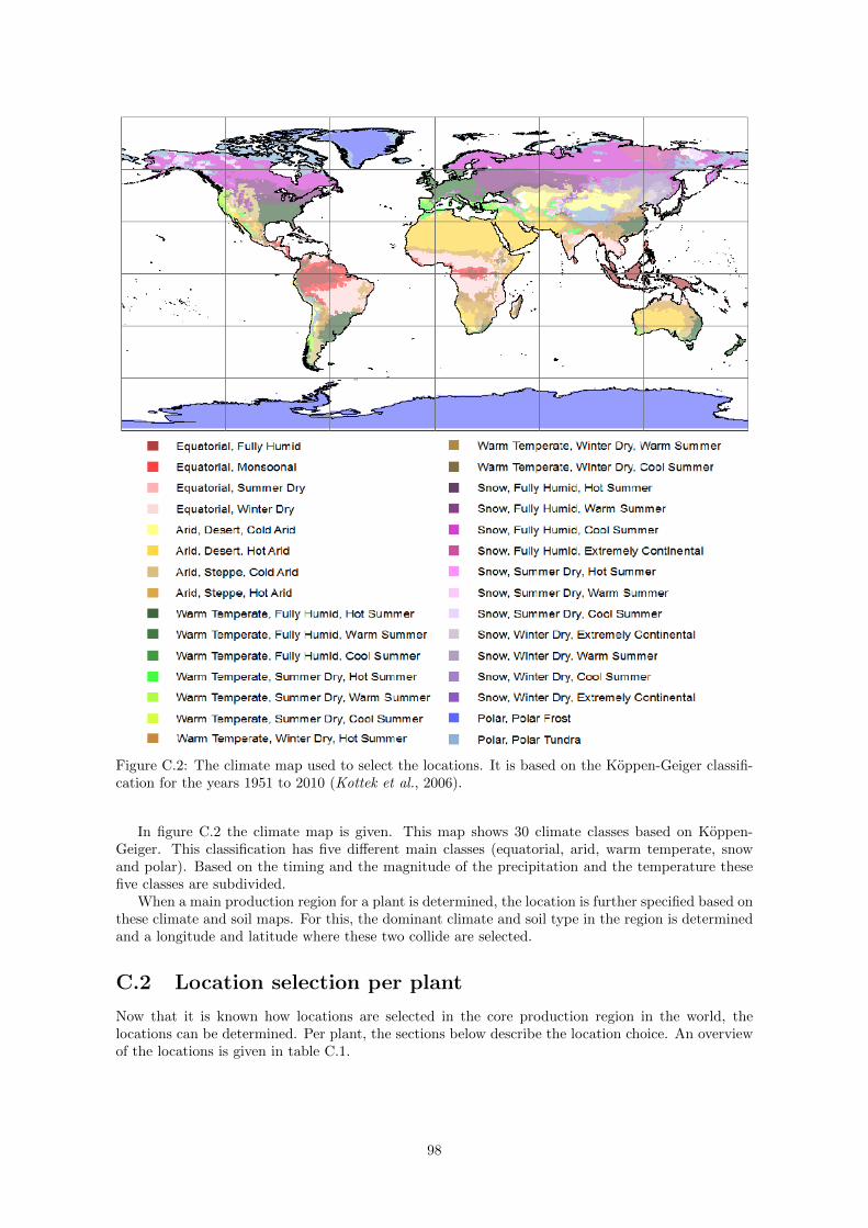
Figure C.2: The climate map used to select the locations. It is based on the Koppen-Geiger classifi-cation for the years 1951 to 2010 (Kottek et al., 2006).

In figure C.2 the climate map is given. This map shows 30 climate classes based on Koppen-Geiger. This classification has five different main classes (equatorial, arid, warm temperate, snowand polar). Based on the timing and the magnitude of the precipitation and the temperature thesefive classes are subdivided.

When a main production region for a plant is determined, the location is further specified based onthese climate and soil maps. For this, the dominant climate and soil type in the region is determinedand a longitude and latitude where these two collide are selected.

C.2 Location selection per plant

Now that it is known how locations are selected in the core production region in the world, thelocations can be determined. Per plant, the sections below describe the location choice. An overviewof the locations is given in table C.1.

98

Table C.1: The locations and their characteristics. The longitude and latitude are in decimal degrees.The climate class refers to the first letters of the climate types in figure C.2, where the part betweenbrackets is the general Koppen-Geiger climate code. The topsoil and subsoil are retrieved from DeLannoy et al. (2014).

Plant Country Province (Lon,Lat) Climate Top-/subsoilApple tree China Shandong (119.16,35.56) WWH (Cwa) 224/55Apple tree Moldova Gagauzia (28.65,46.45) WFW (Cfb) 186/186Apple tree USA Washington (-120.76,46.97) WSW (Csb) 224/40Grapevine Spain Castilla-La Mancha (-2.81,39.31) ASC (BSk) 210/126Olive tree Spain Andalusia (-5.21,36.90) WSH (Csa) 185/16Oil palm Malaysia Johor (103.13,2.25) EF (Af) 207/110

C.2.1 Apple tree

For apple trees, three locations are selected. A global map of apple production is given in figureC.3a. This map shows at which locations the tree is cultivated and at which density. A high densitymeans that there is a large amount of apple trees per unit of area. As can be seen on the map, thecore production of apples in the world takes place in the east of China. This region is therefore alsochosen as the first simulation location for the apple tree. The exact location based on the dominantclimate and soil type in the region is given in table C.1. The corresponding province is Shandong.

To select two alternate locations, there are a few possibilities. First of all, northern India showsa dense apple production. However, the soil types in this region are very fractured and this countryis therefore skipped. Another rather dense apple production is visible north west of the Black Sea,in Moldova. This region has a slightly colder climate and a very different precipitation pattern incomparison to the climate in Shandong. There is a distinct dominant soil type. The details of thislocation are found in table C.1. Furthermore there is some dense apple production visible in the westpart of the United States, in Washington. This region is selected as the third region for the appletree.

C.2.2 Grapevine

Looking at figure C.3b, there are a few locations with a rather dense production of grapevines. InCalifornia in the United States, in eastern Europe and especially around the Mediterranean grapevinesare cultivated quite a lot. There is one region in the world that clearly stands out, namely Castilla-LaMancha in Central Spain. This region is therefore chosen for the grapevine. The specific coordinatesof the locations, the climate type and the soil type can be found in table C.1.

C.2.3 Olive tree

Looking at the map for olive trees in figure C.3c, it can be seen that these trees are grown mainlyaround the Mediterranean. Spain, Morocco, Tunisia, Italy and Israel are visible as rather dense areas.As it is the densest area, the region Andalusia in Spain is chosen as the dominant location of oliveproduction. The details of the location are given in table C.1.

C.2.4 Oil palm

The cultivation of oil palms is mainly reserved for the regions around the equator. In the warmtemperate climates there is some production, but the core production lies in Nigeria and Malaysia.Looking at these locations, Nigeria stands more-or-less on its own when it comes to dense productionof oil palms. Malaysia, on the other hand, is neighboured by the production in Indonesia. WithinMalaysia, the west part has a clear denser production than the east part. Therefore this part ischosen as the representative location for oil palm production. Within West Malaysia, the region ofJohor in the south is chosen. The characteristics at this location can be found in table C.1.

99

(a) Apple tree

(b) Grapevine

(c) Olive tree

Figure C.3: Per plant the places in the world where they are cultivated. The colours show the densityof occurrence (red = high, yellow = low). The maps are retrieved from Monfreda et al. (2008).

100

(d) Oil palm

Figure C.3: (continued) Per plant the places in the world where they are cultivated. The coloursshow the density of occurrence (red = high, yellow = low). The maps are retrieved from Monfredaet al. (2008).

C.3 Reference yield and evapotranspiration

To compare the simulated yields and evapotranspiration rates with reality, it is necessary to find somereference values from literature. In table C.2a, these references are shown for the yield. As can beseen, the main source for the yield is the database of Faostat (2015). This database provides yearlyvalues of the yield on a country level. With these yearly values, the average yield over the period inwhich the plant is considered full-grown can be calculated. More information about the full-grownperiod per plant is found in chapter 3.

For some plants, more location specific information is available. For the apple tree, USDA (2016)provide a database of the yields per year in Washington. The full-grown years of this source aretherefore used. For the apple tree in Shandong, the grapevine and the olive tree, alternate sourceswhere also available, but not for the full-grown period considered in this study. For the period thedata was available, the average is calculated. For these years the average is also calculated with thedata of Faostat (2015). Comparing the two gives a factor that Faostat (2015) over- or underestimatesthe location specific data. This factor is applied on the complete full-grown period by Faostat (2015),resulting in a scaled dataset.

The yield values in literature are reported in fresh weight, while the models simulate yield indry weight. To convert these to each other, the rough estimation proposed by Raes et al. (2012) isused, which states that the dry weight is a quarter of the fresh weight. While this is a very roughapproximation and its applicability is probably not very accurate for all plants considered in thisstudy, no better estimate is available. The values in table C.2a show the dry values of the yield.

The reference values for the evapotranspiration are found in table C.2b. Mekonnen and Hoekstra(2010) provide water footprint data, often on a province level. However, to calculate evapotranspira-tion from the water footprint, also yield is required. Mekonnen and Hoekstra (2010) used the yieldof Faostat for the calculation of water footprint. To calculate the evapotranspiration from the waterfootprint, this study also uses the yield data from Faostat (2015). As these are available on a countrylevel only, also the country level water footprints are used. The evapotranspiration rates are foundby multiplying the water footprints with the yields. For the apple tree in Washington, USBR (2016)provide evapotranspiration data. For the oil palm, Yusop et al. (2008) provide evapotranspirationdata as well. The average of them and Mekonnen and Hoekstra (2010) is used.

101

Table C.2: An overview of the yields and evapotranspiration rates found in literature. The values areas much location specific and for the correct full-grown years as possible. The values of evapotrans-piration are based on the water footprint from Mekonnen and Hoekstra (2010) in combination withthe yields of Faostat (2015). More on this in the text.

(a) Yield

Plant Y [ton/ha] RemarkApple tree (Sh) 4.29 Peng et al. (2008) and Lagos et al. (2009) provide data

for 2004-2008 in Shandong. This is scaled to country data1994-2010 of Faostat (2015)

Apple tree (Ga) 0.97 No better estimate than country data 1994-2010 ofFaostat (2015)

Apple tree (Wa) 9.54 USDA (2016) provide 1995-2010 data for WashingtonGrapevine 0.97 Polytechnic University of Madrid (2005) provide data for

1992-2002 in Castilla-La Mancha. Scaled to country data1981-2010 of Faostat (2015)

Olive tree 0.93 Galan et al. (2008) provide Andalusia average for1990-2004, scaled to country data 2001-2010 of Faostat(2015)

Oil palm 5.00 No better estimate than country data 1998-2009 ofFaostat (2015)

(b) Evapotranspiration

Plant ET [mm/year] RemarkApple tree (Sh) 767 No better estimate than country average of Mekonnen

and Hoekstra (2010)Apple tree (Ga) 548 No better estimate than country average of Mekonnen

and Hoekstra (2010)Apple tree (Wa) 880 USBR (2016) provide data 1988-1999 for WashingtonGrapevine 454 No better estimate than country average of Mekonnen

and Hoekstra (2010)Olive tree 603 No better estimate than country average of Mekonnen

and Hoekstra (2010)Oil palm 1397 Country average of Yusop et al. (2008) and Mekonnen

and Hoekstra (2010)

C.4 Additional soils for further analysis

To compare the influence of different soils on the models, three additional soils are manually selectedfrom De Lannoy et al. (2014). These soils are chosen such that they cover the most extreme soilproperties. The three selected soils are the topsoil/subsoil combination 8/8, 234/234 and 82/172.

Soil 8/8 is characterized by an average saturated hydraulic conductivity, a high field capacity andwilting point and a silty to clayey texture. Soil 234/234 has a high saturated hydraulic conductivity,a low field capacity and wilting point and is rather sandy. Soil 82/172 has a similar texture as soil8/8, but has a very low saturated hydraulic conductivity and an average field capacity and wiltingpoint. The exact parameter values of each of the three soils are found in De Lannoy et al. (2014).

102

Simulating the water footprint of woodies in Aquacrop and Apex

Documents