Simulating quantum-optical phenomena with cold atoms in

OPEN ACCESS

Simulating quantum-optical phenomena with coldatoms in optical latticesTo cite this article: Carlos Navarrete-Benlloch et al 2011 New J. Phys. 13 023024

View the article online for updates and enhancements.

You may also likeSecurity analysis of an untrusted sourcefor quantum key distribution: passiveapproachYi Zhao, Bing Qi, Hoi-Kwong Lo et al.

-

Irreducible many-body correlations intopologically ordered systemsYang Liu, Bei Zeng and D L Zhou

-

Limitations of rotating-wave approximationin magnetic resonance: characterizationand elimination of the Bloch–Siegert shiftin magneto-opticsJ I Sudyka, S Pustelny and W Gawlik

-

Recent citationsQuantum electrodynamics in anisotropicand tilted Dirac photonic latticesJaime Redondo-Yuste et al

-

Sub-wavelength spin excitations inultracold gases created by stimulatedRaman transitionsYigal Ilin et al

-

Effective many-body Hamiltonians of qubit-photon bound statesT Shi et al

-

This content was downloaded from IP address 118.106.121.34 on 14/11/2021 at 01:13

T h e o p e n – a c c e s s j o u r n a l f o r p h y s i c s

New Journal of Physics

Simulating quantum-optical phenomena with coldatoms in optical lattices

Carlos Navarrete-Benlloch1,4, Inés de Vega2, Diego Porras3 andJ Ignacio Cirac4

1 Departament d’Òptica, Universitat de València, Dr Moliner 50,46100 Burjassot, Spain2 Institut für Theoretische Physik, Albert-Einstein-Allee 11, Universität Ulm,D-89069 Ulm, Germany3 Departamento de Física Teórica I, Universidad Complutense, 28040 Madrid,Spain4 Max-Planck-Institut für Quantenoptik, Hans-Kopfermann-Strasse 1,85748 Garching, GermanyE-mail: [email protected], [email protected],[email protected] and [email protected]

New Journal of Physics 13 (2011) 023024 (23pp)Received 8 October 2010Published 10 February 2011Online at http://www.njp.org/doi:10.1088/1367-2630/13/2/023024

Abstract. We propose a scheme involving cold atoms trapped in optical latticesto observe different phenomena traditionally linked to quantum-optical systems.The basic idea consists of connecting the trapped atomic state to a non-trappedstate through a Raman scheme. The coupling between these two types ofatoms (trapped and free) turns out to be similar to that describing light–matterinteraction within the rotating-wave approximation, the role of matter andphotons being played by the trapped and free atoms, respectively. We explainin particular how to observe phenomena arising from the collective spontaneousemission of atomic and harmonic oscillator samples, such as superradianceand directional emission. We also show how the same setup can simulateBose–Hubbard Hamiltonians with extended hopping as well as Ising modelswith long-range interactions. We believe that this system can be realized withstate of the art technology.

New Journal of Physics 13 (2011) 0230241367-2630/11/023024+23$33.00 © IOP Publishing Ltd and Deutsche Physikalische Gesellschaft

2

Contents

1. Introduction 22. The model 43. Emission of an atom from a single site 64. Collective dynamics 8

4.1. Extended Bose–Hubbard and spin models . . . . . . . . . . . . . . . . . . . . 94.2. Dicke superradiance . . . . . . . . . . . . . . . . . . . . . . . . . . . . . . . . 104.3. Directional superradiance . . . . . . . . . . . . . . . . . . . . . . . . . . . . . 15

5. Considerations about dimensionality 166. Conclusions 16Acknowledgments 18Appendix A. Extracting information from the non-Markovian equation (7) 18Appendix B. Evaluation of the Markov couplings (13) 22References 22

1. Introduction

Cold atoms trapped in optical lattices have been proved to be very versatile quantum systems inwhich a large class of many-body condensed matter Hamiltonians can be simulated (see [1]–[3]for extensive reviews on this subject). One of the first proposals in this direction was the articleby Jacksch et al [4], where it was proved that the dynamics of cold atoms trapped in opticallattices is described by the Bose–Hubbard Hamiltonian provided that certain conditions aresatisfied; shortly after, the superfluid-to-Mott insulator phase transition characteristic of thisHamiltonian was observed in the laboratory [5]. Since then, the broad tunability of the latticeparameters, and the increasing ability to trap different kinds of particles (such as bosonic andfermionic atoms with arbitrary spin or polar molecules), has allowed theoreticians to proposeoptical lattices as promising simulators for different types of generalized Bose–Hubbard andspin models that are in close relation to important condensed-matter phenomena [1]–[3].Recent experiments have shown that optical lattices can be used to address open problems inphysics such as high-Tc superconductivity [6], to study phenomena in low dimensions suchas the Berezinskii–Kosterlitz–Thouless transition [7] or to implement quantum computationschemes [8].

In this paper, we keep digging into the capabilities of optical lattices as simulators, showinghow they can also be a powerful tool for simulating quantum-optical phenomena. In particular,following our previous proposal [9], we introduce various schemes in which superradiance-like phenomena can be observed. In addition, we will show that these same schemes realizeBose–Hubbard and spin models with extended interactions (in particular, models where hoppingbetween sites and ferromagnetic interactions between spins are long-range instead of nearestneighbors).

The concept of superradiance was introduced by Dicke in 1954 when studying thespontaneous emission of a collection of two-level atoms [10] (see [11] for a review). Heshowed that certain collective states where the excitations are distributed symmetrically overthe whole sample have enhanced emission rates. Probably the most stunning example is the

New Journal of Physics 13 (2011) 023024 (http://www.njp.org/)

3

single-excitation symmetric state (now known as the symmetric Dicke state), which, insteadof decaying with the single-atom decay rate 00, was shown to decay with N00, N being thenumber of atoms. He also suggested that the emission rate of the state having all the atomsexcited should be enhanced at the initial steps of the decay process, which was a very interestingprediction from the experimental point of view, as this state is in general easier to prepare.However, Dicke used a very simplified model in which all the atoms interact with a commonradiation field within the dipolar approximation; almost 15 years later, and motivated by the newatom-inversion techniques, several authors showed that dipolar interactions impose a thresholdvalue for the atom density, that is, for the number of interacting atoms, in order for superradianceto appear [12]–[14].

It is worth noting that together with atomic ensembles, spontaneous emission of collectionsof harmonic oscillators were also studied at that time [13]. Two interesting features of this sys-tem were reported: (i) an initial state with all of the harmonic oscillators excited does not showrate enhancement; on the contrary, most excitations remain within the sample in the steady state,while (ii) the state having all of the oscillators in the same coherent state has a superradiant rate.

In recent years, there has been renewed interest in this phenomenology because of itspotential for quantum technologies [15]–[20]. In these new approaches, superradiant effectsdiffer from those found by Dicke in that they are mediated by the initial entanglement of theemitters, not by a buildup of their coherence. Of particular interest to the present work is theanalysis performed in [18] (see also [17]) of the spontaneous emission by regular arrays ofatoms separated by a distance d0 comparable to the wavelength λ of the emitted radiation. Itwas shown that directional emission can be obtained for particular single-excitation entangledstates when λ > 2d0, the emission rate being enhanced by a factor χ ∝ (λ/d0)

2 N 1/3.Also of interest for our purposes is the work carried out by Sajeev John and

collaborators [21, 22] on the collective emission of atoms embedded in photonic band-gapmaterials. In this kind of material, the density of states of the electromagnetic field is zero forfrequencies lying within the gap, which gives rise to the phenomenon of light localization [23].As for collective emission, it was shown by using a simplified Dicke-like model [21, 22] thatwhen the atomic transition lies close to the gap, radiation is emitted in the form of evanescentwaves and the single-excitation symmetric state has a rate proportional to N 200, which is evenlarger than the one predicted by Dicke in free space.

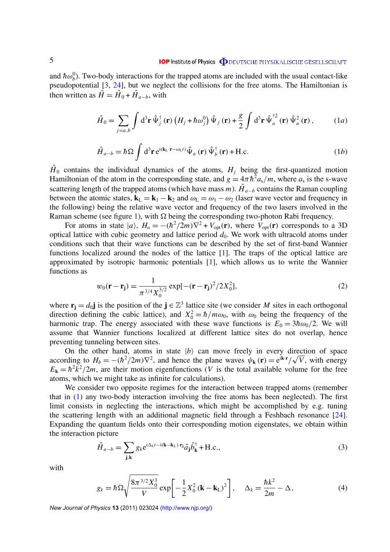
We will show that all of this phenomenology can be observed in optical lattices with thesetup already presented in [9], which is depicted in figure 1. Consider a collection of bosonicatoms with two relevant internal states labeled a and b (which may correspond to hyperfineground-state levels, see for example [1]). Atoms in state a are trapped by a deep optical latticein which the localized wave function of traps at different lattice sites do not overlap (preventinghopping of atoms between sites), while atoms in state b are not affected by the lattice and hencebehave as free particles. A pair of lasers forming a Raman scheme drives the atoms from thetrapped state to the free one [1], providing an effective interaction between the two types ofparticles. We consider the situation of having non-interacting bosons in the lattice [24], as wellas hard-core bosons in the collisional blockade regime, where only one or zero atoms can bein a given lattice site [25]. In the first regime, the lattice consists of a collection of harmonicoscillators placed at the nodes of the lattice; in the second regime, two-level systems replace theharmonic oscillators, the two levels corresponding to the absence or presence of an atom in thelattice site. Therefore, it is apparent that this system is equivalent to a collection of independentemitters (harmonic oscillators or atoms) connected only through a common radiation field,

New Journal of Physics 13 (2011) 023024 (http://www.njp.org/)

4

Figure 1. Scheme of our proposed setup. Atoms in state a are trapped in anoptical lattice, while atoms in state b are free, and can thus have any momentum.An external pair of Raman lasers connect the two levels with some detuning 1.We will show that above some critical value1=1c, the atoms in state b are ableto leave the trap (left), whereas below this, they are trapped forming a bound statewith atoms in state a (right). This behavior is typical of band-gap systems wherethe density of states is zero between the connected states.

the role of this radiation field being played by the free atoms. This system is therefore thecold-atom analogue of the quantum-optical systems considered above, with the difference thatthe radiated particles are massive and hence have a different dispersion relation than that ofphotons in vacuum. Moreover, we show that the field of free atoms can be characterized by adispersion relation that is similar to the one obtained for photons within a photonic band-gapmaterial [9, 21, 22]. It is then to be expected, and so we will prove, that this system will showthe same kind of phenomenology as its quantum-optical counterparts.

Note that the hard-core boson case was already discussed in [9], and hence, apart from amore detailed discussion of the results that can be found there, the main new results of this paperare those concerning non-interacting bosons.

To conclude this introduction, let us explain how the paper is organized. We first introducethe model and find its associated Hamiltonian (section 2). Then we study the radiative propertiesof the system when the lattice sites emit independently (section 3); we will show in this sectionthat our system shows localization of the free atoms, in analogy to the localization of lightoccurring in a photonic band-gap material, and we identify as well the Markovian and non-Markovian regimes of the emission. In section 4, we study collective effects. We first deducea reduced master equation for the lattice atoms, explaining under what conditions it is valid.We then show how by changing the system parameters, extended Bose–Hubbard and spinmodels (section 4.1), Dicke superradiance of atomic (section 4.2.1) and harmonic oscillator(section 4.2.2) samples, and directional superradiance (section 4.3) can be observed. We finallytalk about the effect of restricting the motion of the free atoms to two-dimensional (2D) or 1Dtraps in section 5, and present some conclusions in section 6.

2. The model

Our starting point is the Hamiltonian of the system in second quantization [26]. We will denoteby |a〉 and |b〉 the trapped and free atomic states, respectively (having internal energies hω0

a

New Journal of Physics 13 (2011) 023024 (http://www.njp.org/)

5

and hω0b). Two-body interactions for the trapped atoms are included with the usual contact-like

pseudopotential [3, 24], but we neglect the collisions for the free atoms. The Hamiltonian isthen written as H = H 0 + H a−b, with

H 0 =

∑j=a,b

∫d3r 9†

j (r)(H j + hω0

j

)9 j (r)+

g

2

∫d3r 9

†2

a (r) 92a (r) , (1a)

H a−b = h�∫

d3r ei(kL·r−ωLt)9a (r) 9†b (r)+ H.c. (1b)

H 0 contains the individual dynamics of the atoms, H j being the first-quantized motionHamiltonian of the atom in the corresponding state, and g = 4π h2as/m, where as is the s-wavescattering length of the trapped atoms (which have mass m). H a−b contains the Raman couplingbetween the atomic states, kL = k1 − k2 and ωL = ω1 −ω2 (laser wave vector and frequency inthe following) being the relative wave vector and frequency of the two lasers involved in theRaman scheme (see figure 1), with � being the corresponding two-photon Rabi frequency.

For atoms in state |a〉, Ha = −(h2/2m)∇2 + Vopt(r), where Vopt(r) corresponds to a 3Doptical lattice with cubic geometry and lattice period d0. We work with ultracold atoms underconditions such that their wave functions can be described by the set of first-band Wannierfunctions localized around the nodes of the lattice [1]. The traps of the optical lattice areapproximated by isotropic harmonic potentials [1], which allows us to write the Wannierfunctions as

w0(r − rj)=1

π 3/4 X 3/20

exp[−(r − rj)2/2X 2

0], (2)

where rj = d0j is the position of the j ∈ Z3 lattice site (we consider M sites in each orthogonaldirection defining the cubic lattice), and X 2

0 = h/mω0, with ω0 being the frequency of theharmonic trap. The energy associated with these wave functions is E0 = 3hω0/2. We willassume that Wannier functions localized at different lattice sites do not overlap, hencepreventing tunneling between sites.

On the other hand, atoms in state |b〉 can move freely in every direction of spaceaccording to Hb = −(h2/2m)∇2, and hence the plane waves ψk (r)= eik·r/

√V , with energy

Ek = h2k2/2m, are their motion eigenfunctions (V is the total available volume for the freeatoms, which we might take as infinite for calculations).

We consider two opposite regimes for the interaction between trapped atoms (rememberthat in (1) any two-body interaction involving the free atoms has been neglected). The firstlimit consists in neglecting the interactions, which might be accomplished by e.g. tuningthe scattering length with an additional magnetic field through a Feshbach resonance [24].Expanding the quantum fields onto their corresponding motion eigenstates, we obtain withinthe interaction picture

H a−b =

∑j,k

gkei1k t−i(k−kL )·rj ajb†k + H.c., (3)

with

gk = h�

√8π3/2 X 3

0

Vexp

[−

1

2X 2

0 (k − kL)2

], 1k =

hk2

2m−1, (4)

New Journal of Physics 13 (2011) 023024 (http://www.njp.org/)

6

where 1= ωL − (ωb −ωa) is the detuning of the laser frequency with respect to the |a〉 |b〉

transition (ωa = ω0a + 3ω0/2 and ωb = ω0

b). The operators {aj, a†j } and {bk, b†

k} satisfy canonicalbosonic commutation relations, and create or annihilate an atom at lattice site j and a free atomwith momentum k, respectively.

As for the second limit, we assume that the on-site repulsive atom–atom interaction isthe dominant energy scale, and hence the trapped atoms behave as hard-core bosons in thecollisional blockade regime, which prevents the presence of two atoms in the same latticesite [25]; this means that the spectrum of a†

j aj can be restricted to the first two states {|0〉j, |1〉j},

having 0 or 1 atom at site j, and then the boson operators {a†j , aj} can be changed by spin-like

ladder operators {σ†j , σ j} = {|1〉j〈0|, |0〉j〈1|}. In this second limit, the Hamiltonian reads

H a−b =

∑j,k

gkei1k t−i(k−kL)·rj σ jb†k + H.c. (5)

Hamiltonians (3) and (5) show explicitly how this system mimics the dynamics ofcollections of harmonic oscillators or atoms, respectively, interacting with a common radiationfield. Note that, particularly, the dispersion relation appearing in (4) is similar to that of theradiation field within an anisotropic 3D photonic band-gap material, where photons acquirean effective mass close to the gap [21, 22]. We will show how by varying the parameters ofthese Hamiltonians, the system has access to regimes showing many different phenomena, asexplained in the introduction.

Note, finally, that to satisfy that the trapped atoms are within the first Bloch band, it isrequired that ω0 �1,�.

3. Emission of an atom from a single site

Before studying the collective behavior of the atoms in the lattice, it is convenient to understandthe different regimes of emission when the sites emit independently. To this end, we first studythe emission properties of one atom in a single site following the analysis performed in [21, 22]for an atom embedded in a photonic band-gap material. We are going to show that there exists acritical value of the detuning above which the atom is emitted, while below which the radiatedatom gets bound to the trapped atom, and there is a non-zero probability for the atom to remainin the trap (see figure 1). This second regime is the analogue of the photon–atom bound statepredicted more than 25 years ago [23]. We will also identify the Markovian and non-Markovianregimes of the emission.

Following the Weisskopf–Wigner procedure [27, 28], we write the state of an atom in asingle site (which we take as j = 0) as

|ψ (t)〉 = A (t) |1, {0}〉 +∑

k

Bk (t) |0, 1k〉, (6)

where |1, {0}〉 refers to the state with an atom in the trap and no free atoms, and |0, 1k〉 refersto the state with no trapped atoms and one free atom with momentum k. We can use theSchrödinger equation to write the evolution equations of the coefficients A and Bk; then, theequation of Bk can be formally integrated arriving at a single equation for A given by

A (t)= −

∫ t

0dt ′ G(t − t ′)A(t ′), (7)

New Journal of Physics 13 (2011) 023024 (http://www.njp.org/)

7

where we have assumed that the atom is initially in the trap; that is, A(0)= 1 and Bk(0)= 0.This is a non-Markovian equation where the free atoms enter the dynamics of the trapped atomsas a reservoir with the correlation function

G (τ )=1

h2

∑k

|gk|2 e−i1kτ =

�2

(1 + (i/2)ω0τ)3/2 exp (i1τ), (8)

where we have taken the continuous limit for the momenta in the last equality and kL = 0 forsimplicity. Note that this correlation function coincides exactly with that of atoms in anisotropic3D photonic band-gap materials [21, 22].

In appendix A, we show how to handle equation (7) by using Laplace transform techniques.In particular, in appendix A.1 we show that in the strong confinement regime ω0 → ∞, thisequation can be solved as

A (t)= cei(b2+1)t +2α√π

eiπ/4

∫ +∞

0dx

√x e(−x+i1)t

(−x + i1)2 + i4πα2x, (9)

with α2= 8�4/ω3

0, 1=1− 4�2/ω0 andc = 2b+/ (b+ − b−) and b = b+ for 1 < 0,

c = 0, for 0< 1 < πα2,

c = 2b−/ (b− − b+) andb = b− for 1 > πα2,

(10)

where b± =√πα(−1 ±

√1 − 1/πα2).

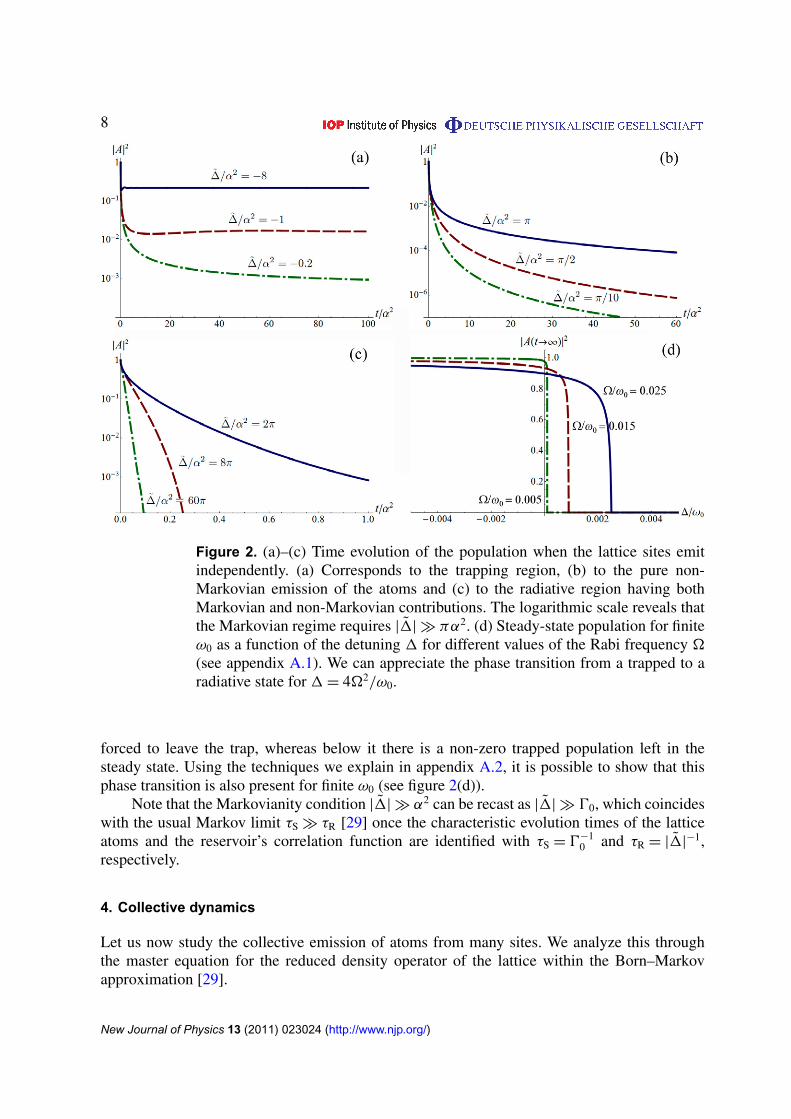
Solution (9) has a very suggestive form. The first term has exponential evolution asexpected for a Markovian radiation process, while the integral term has a non-trivial timedependence that always goes to zero for sufficiently large times. The time while the integralterm is comparable to the exponential one defines the non-Markovian part of the evolution. Thisresult also shows that the behavior of the emission is highly dependent on the parameters of thesystem:

• In the 1 < 0 region Im{b2+} = 0, and hence the steady-state population is non-zero and

given by |A(t → ∞)|2 = |c|2 = (1 − 1/√

1 + |1|/πα2)2; a fraction 1 − |c|2 is radiated

during the non-Markovian period that lasts longer as 1/α2 goes to zero (see figure 2(a)).In this region, the radiated atoms are emitted in the form of evanescent waves, and theequivalent of a photon–atom bound state [23] is formed.

• In the 0< 1 < πα2 region (figure 2(b)), the steady-state population is zero, i.e. the atomleaves the trap eventually, and the evolution is dictated solely by the integral part of thesolution (hence it is pure non-Markovian radiation).

• Finally, in the 1 > πα2 region, the atom is radiated in a Markovian fashion only for

1� α2, with a decay rate given by 00 = Im{b2−} ≈ 4�2

√2π1/ω3

0; if this is not the

case (1∼ α2), the integral part is comparable to the exponential part during most of theevolution time, and hence the radiation process is non-Markovian (figure 2(c)).

Therefore, there exists a phase transition at 1= 4�2/ω0 in close analogy to that ofspontaneous emission in photonic band-gap materials [21, 22]. Above this value, the atom is

New Journal of Physics 13 (2011) 023024 (http://www.njp.org/)

8

Figure 2. (a)–(c) Time evolution of the population when the lattice sites emitindependently. (a) Corresponds to the trapping region, (b) to the pure non-Markovian emission of the atoms and (c) to the radiative region having bothMarkovian and non-Markovian contributions. The logarithmic scale reveals thatthe Markovian regime requires |1| � πα2. (d) Steady-state population for finiteω0 as a function of the detuning 1 for different values of the Rabi frequency �(see appendix A.1). We can appreciate the phase transition from a trapped to aradiative state for 1= 4�2/ω0.

forced to leave the trap, whereas below it there is a non-zero trapped population left in thesteady state. Using the techniques we explain in appendix A.2, it is possible to show that thisphase transition is also present for finite ω0 (see figure 2(d)).

Note that the Markovianity condition |1| � α2 can be recast as |1| � 00, which coincideswith the usual Markov limit τS � τR [29] once the characteristic evolution times of the latticeatoms and the reservoir’s correlation function are identified with τS = 0−1

0 and τR = |1|−1,

respectively.

4. Collective dynamics

Let us now study the collective emission of atoms from many sites. We analyze this throughthe master equation for the reduced density operator of the lattice within the Born–Markovapproximation [29].

New Journal of Physics 13 (2011) 023024 (http://www.njp.org/)

9

We introduce the Born approximation by fixing the state of the reservoir to a non-evolvingvacuum. This leads to an effective interaction between different lattice sites mediated by thetwo-point correlation function5,

Gj−l (τ )=1

h2

∑k

g2k e−i1kτ+i(k−kL)·rj−l〈bkb†

k〉 = exp

(−r 2

j−l/4X 20

1 + iω0τ/2− ikL · rj−l

)G (τ ), (11)

where rj−l = rj − rl = d0(j − l). The Born approximation yields the dynamics of the system toleading order in the coupling parameters gk [29]. On the other hand, as mentioned at the end ofthe previous section, the Markov approximation is valid only if |1| � 0, where 0 is a typicalevolution rate for trapped atoms, which can differ from 00 owing to a renormalization due tocollective effects, as we show below. We also include the single-site energy shift that we foundin the previous section (the analogue of the Lamb shift in the optical case), and substitute 1 by1 in the two-point correlation function.

The master equation for the reduced density operator of the trapped atoms ρ is found byusing standard techniques from the theory of open quantum systems [29], and reads

dρ

dt=

∑j,l

0j−lalρa†j −0j−la

†j alρ + H.c.; (12)

a similar equation is obtained for the hard-core bosons but replacing the boson operators bythe corresponding spin operators. The effective interaction between different lattice sites ismediated by the Markov couplings (see appendix B)

0j−l = i exp(−ikL · rj−l)00ξ

|j − l|

[1 − erf

(d0

2X0|j − l|

)− exp

(−ν

|j − l|ξ

)], (13)

where ξ = 1/d0k0 with k0 = X−10

√2|1|/ω0 measures the ratio between the lattice spacing and

the characteristic wavelength of the radiated atoms, and ν = 1 (−i) for 1 < 0 (1 > 0). The errorfunction is defined as erf(x)= (2/

√π)∫ x

0 du exp(−u2). This expression has been evaluated inthe strong confinement regime ω0 → ∞ and considering kL � X−1

0 (see appendix B). Notethat the term ‘1 − erf(d0|j − l|/2X0)’ is basically zero for j 6= l, and therefore the ξ parameterdictates the spatial range of the interactions, as can be appreciated in figure 3. Finally, we recall

that 00 = 4�2√

2π |1|/ω30 is the single-emitter decay rate.

4.1. Extended Bose–Hubbard and spin models

For kL = 0 and 1 < 0, the Markov couplings are purely imaginary and have negative imaginaryparts. Under these conditions, the master equation takes a Hamiltonian form with effectiveHamiltonians

H eff = −

∑j,l

h∣∣0j−l

∣∣ a†j al and H eff = −

∑j,l

h∣∣0j−l

∣∣ σ †j σ l, (14)

for non-interacting and hard-core bosons, respectively. The first Hamiltonian describes extendedhopping in the lattice, a feature that has been recently shown to be helpful for achieving true

5 Note that equations (11) and (13) correct some typos that can be found in equations (4) and (5) of our previouspaper [9].

New Journal of Physics 13 (2011) 023024 (http://www.njp.org/)

10

Figure 3. We plot the Markov couplings (real and imaginary parts on the leftand right, respectively) as a function of the distance between sites for 1 > 0. Wehave chosen d0/X0 = 10 and kL = 0 and plotted four different values of ξ . It canbe appreciated that this parameter controls the spatial range of the interactions.

incompressible Mott phases that otherwise can be blurred because of the additional slowlyvarying harmonic trap used to confine the atoms within the lattice [30]. The second Hamiltonianis equivalent to an extended ferromagnetic Ising-like Hamiltonian, and it connects our systemto extended spin models. Note that for j 6= l the couplings have a Yukawa form,∣∣0j−l

∣∣≈ 00

|j − l| /ξexp

(−

|j − l|ξ

), (15)

and can even take a Coulomb form if ξ is large enough. These kinds of interactions (especiallythe Coulomb-like) are difficult to obtain with other techniques.

These results show that in the trapping region the system under study could be useful forquantum simulation of condensed matter phenomena requiring extended interactions.

4.2. Dicke superradiance

In this section, we connect our system to superradiant Dicke-like phenomena both in atomic andharmonic oscillator samples (we will still take kL = 0).

For 1 > 0, the Markov couplings are complex in general and therefore the master equationof the system takes the form

dρ

dt=

1

ih[H d, ρ] +D[ρ], (16)

with a dissipation term given by

D[ρ]=

∑j,l

γj−l

(2alρa†

j − a†j alρ− ρa†

l aj

), (17)

having collective decay rates

γj−l = Re{0j−l} = 00 sinc

(|j − l|ξ

), (18)

New Journal of Physics 13 (2011) 023024 (http://www.njp.org/)

11

and a reversible term corresponding to inhomogeneous dephasing with Hamiltonian

H d =

∑j,l

h3j−la†j al, (19)

where

3j−l = Im{0j−l} =00ξ

|j − l|

[1 − erf

(d0

2X0|j − l|

)− cos

(|j − l|ξ

)]. (20)

The same holds for hard-core bosons but replacing the boson operators by the correspondingspin operators.

For ξ � 1, the Markov couplings do not connect different lattice sites, that is, 0j−l ' 00δj,l,and the sites emit independently. On the other hand, when ξ � M , the collective decay ratesbecome homogeneous, γj−l ' 00, and we enter the Dicke regime. Hence, we expect to observethe superradiant phase transition in our system by varying the parameter ξ .

Note that in the Dicke regime the dephasing term cannot be neglected and connectsthe sites inhomogeneously with 3j6=l ' 00ξ/|j − l|. This term appears in the optical case too,although it was inappropriately neglected in the original work by Dicke [10] when assuming thedipolar approximation in his initial Hamiltonian, and slightly changes his original predictions,as pointed out in [31, 32] (see also [11]).

In the following, we analyze the superradiant behavior of our system by studying theevolution of the total number of particles in the lattice nT =

∑j〈a

†j aj〉 and the rate of emitted

atoms

R (t)=

∑k

d

dt〈b†

kbk〉 = −dnT

dt; (21)

in the last equality, we have used the fact that the total number operator∑

k b†kbk +

∑j a†

j aj is aconstant of motion.

4.2.1. Hard-core bosons: atomic superradiance. Let us start by analyzing the case of a latticein an initial Mott phase having one atom per site in the collisional blockade regime, which is theanalogue of an ensemble of excited atoms [9]. As explained in the introduction, Dicke predictedthat superradiance should appear in this system as an enhancement of the emission rate at earlytimes [10], although this was later proved to happen only if the effective number of interactingemitters exceeds some threshold value [12]–[14]. This is the superradiant phase transition.

In our system, the number of interacting spins is governed by the parameter ξ (see figure 3),and the simplest way to show that the superradiant phase transition appears by varying it is byevaluating the initial slope of the rate, which can be written as6

d

dtR∣∣∣∣t=0

= −4M3020

1 −

∑m6=j

sinc2(|j − m| /ξ)

M3

. (23)

6 Note that the evolution equation of the expectation value of any operator O can be written as

d

dt〈O(t)〉 = tr

{dρ

dtO

}= −

∑m,l

{0m−l〈[O, a†m]al〉 +0∗

m−l〈a†l [am, O]〉}, (22)

and similarly for hard-core bosons in terms of the spin ladder operators.

New Journal of Physics 13 (2011) 023024 (http://www.njp.org/)

12

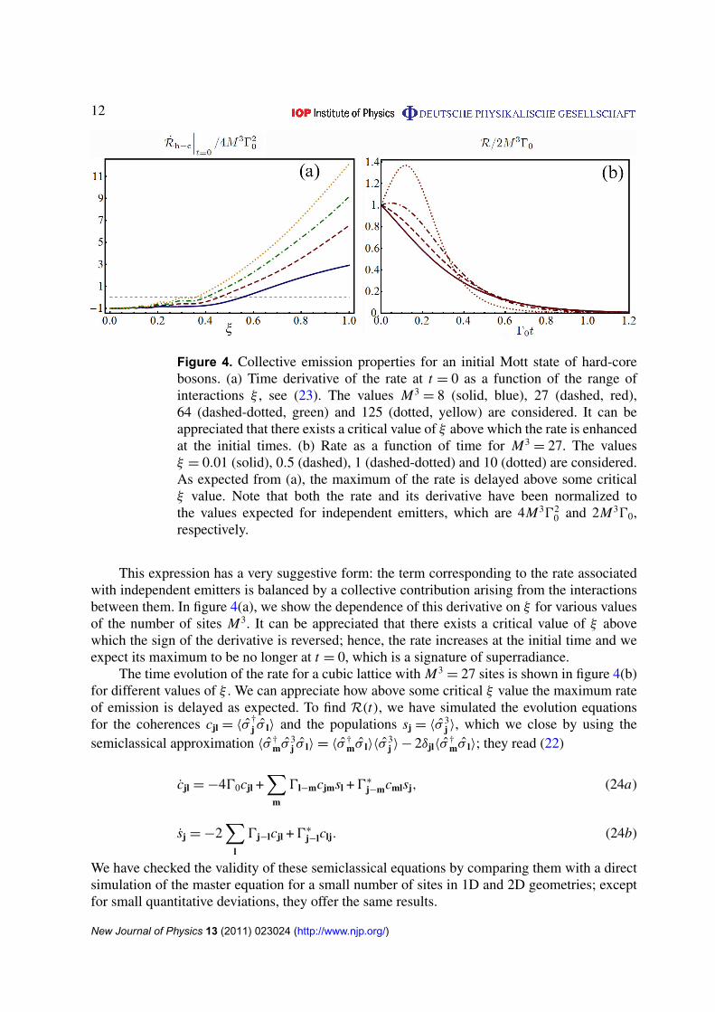
Figure 4. Collective emission properties for an initial Mott state of hard-corebosons. (a) Time derivative of the rate at t = 0 as a function of the range ofinteractions ξ , see (23). The values M3

= 8 (solid, blue), 27 (dashed, red),64 (dashed-dotted, green) and 125 (dotted, yellow) are considered. It can beappreciated that there exists a critical value of ξ above which the rate is enhancedat the initial times. (b) Rate as a function of time for M3

= 27. The valuesξ = 0.01 (solid), 0.5 (dashed), 1 (dashed-dotted) and 10 (dotted) are considered.As expected from (a), the maximum of the rate is delayed above some criticalξ value. Note that both the rate and its derivative have been normalized tothe values expected for independent emitters, which are 4M302

0 and 2M300,respectively.

This expression has a very suggestive form: the term corresponding to the rate associatedwith independent emitters is balanced by a collective contribution arising from the interactionsbetween them. In figure 4(a), we show the dependence of this derivative on ξ for various valuesof the number of sites M3. It can be appreciated that there exists a critical value of ξ abovewhich the sign of the derivative is reversed; hence, the rate increases at the initial time and weexpect its maximum to be no longer at t = 0, which is a signature of superradiance.

The time evolution of the rate for a cubic lattice with M3= 27 sites is shown in figure 4(b)

for different values of ξ . We can appreciate how above some critical ξ value the maximum rateof emission is delayed as expected. To find R(t), we have simulated the evolution equationsfor the coherences cjl = 〈σ

†j σ l〉 and the populations sj = 〈σ 3

j 〉, which we close by using thesemiclassical approximation 〈σ †

mσ3j σ l〉 = 〈σ †

mσ l〉〈σ3j 〉 − 2δjl〈σ

†mσ l〉; they read (22)

cjl = −400cjl +∑

m

0l−mcjmsl +0∗

j−mcmlsj, (24a)

sj = −2∑

l

0j−lcjl +0∗

j−lclj. (24b)

We have checked the validity of these semiclassical equations by comparing them with a directsimulation of the master equation for a small number of sites in 1D and 2D geometries; exceptfor small quantitative deviations, they offer the same results.

New Journal of Physics 13 (2011) 023024 (http://www.njp.org/)

13

4.2.2. Non-interacting bosons: harmonic oscillators superradiance. Let us analyze now thecase of having non-interacting bosons in the lattice, which is equivalent to a collection ofharmonic oscillators, as discussed before. In previous works on superradiance, this system wasstudied in parallel with its atomic counterpart [13], and here we show how our system offers aphysical realization of it. We will show that superradiant effects can be observed in the evolutionof the total number of atoms in the lattice, for both initial Mott and superfluid phases7.

The evolution of the total number of atoms in the lattice is given by (see (22))

nT = −2∑

j,l

γj−lRe{〈a†j al〉}, (26)

and hence depends only on the real part of the Markov couplings. Therefore, we restrict ouranalysis to the dissipative term D[ρ] of the master equation (16).

By diagonalizing the real, symmetric collective decay rates with an orthogonal matrix Ssuch that

∑jlSpjγj−lSql = γpδpq, one can find a set of modes {cp =

∑j Spjaj} with definite decay

properties. Then, it is completely straightforward to show that the total number of atoms can bewritten as a function of time as

nT (t)=

∑p

〈c†pcp (0)〉 exp(−2γpt). (27)

In general, γj−l requires numerical diagonalization. However, in the limiting cases ξ � 1and ξ � M , its spectrum becomes quite simple. Following the discussion after (20), in theξ � 1 limit, γj−l = 00δjl is already diagonal and proportional to the identity. Hence, anyorthogonal matrix S defines an equally suited set of modes all decaying with rate 00. Therefore,if the initial number of atoms in the lattice is N , this will evolve as

nT (t)= N exp(−200t), (28)

irrespective of the particular initial state of the lattice (e.g. Mott or superfluid). The emissionrate R= 200 N exp(−200t) corresponds to the independent decay of the N atoms as expectedin this regime having no interaction between the emitters.

Let us consider now the opposite limit ξ � M ; in this case γj−l = 00 ∀ (j, l), and thedissipative term can be written in terms of the symmetrical discrete Fourier-transform mode onlyasD

[ρ]= M300(2 f 0ρ f †

0 − f †0 f 0ρ− f †

0 f 0ρ) (see (25)). Hence, the discrete Fourier-transformbasis diagonalizes the problem, and shows that all of the modes have zero decay rate except thesymmetrical one, which has an enhanced rate proportional to the number of emitters. Therefore,starting with a superfluid state, the N initial atoms will decay exponentially with initial rateN M300, that is,

nT (t)= N exp(−2M300t). (29)

On the other hand, if the initial state corresponds to a Mott phase, most of the atoms will remainin the lattice, as only the component that projects onto the symmetric mode will be emitted;

7 Let us note that a superfluid state with N excitations distributed over the entire lattice is more easily defined inthe discrete Fourier-transform basis,

f q =1

M3/2

∑j

exp

(2π i

Mq · j

)aj, (25)

with q = (qx , qy, qz) and qx,y,z = 0, 1, 2, . . . ,M − 1, as the state having N excitations in the zero-momentummode; that is, |SF〉N = (N !)−1/2 f †N

0 |0〉.

New Journal of Physics 13 (2011) 023024 (http://www.njp.org/)

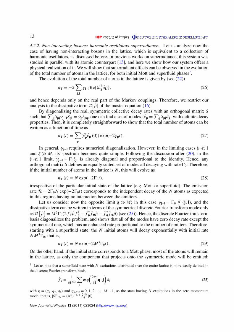
14

Figure 5. Evolution of the total number of atoms in a lattice having M3= 27

sites for initial superfluid (a) and Mott (b) phases with N initial non-interactingatoms. The solid curves correspond to the limits ξ � 1 (gray) and ξ � M (darkblue). Note how the ‘evaporation time’ is reduced for the initial superfluid stateas ξ increases (a). Equivalently, note how for an initial Mott state the atoms tendto stay in the lattice as ξ increases (b).

concretely, from (27) and (25) the number of atoms in the lattice will evolve for this particularinitial state as

nT (t)=

(N −

N

M3

)+

N

M3exp

(−2M300t

). (30)

Hence, according to this picture, superradiant collective effects can be observed in oursystem by two different means. Calling t0 the time needed to radiate the atoms in the absenceof collective effects, one could start with a superfluid phase and measure this ‘evaporation time’as a function of ξ ; this should go from t0 for ξ � 1, to a much shorter time t0/M3 for ξ � M(see figure 5(a)). Alternatively, one could start with a Mott phase, and measure the number ofatoms left in the lattice in the steady state as a function of ξ ; in this case, it should go fromnT,steady = 0 after a time t0 for ξ � 1, to nT,steady = N − N/M3 after a time t0/M3 for ξ � M(see figure 5(b)).

To find the evolution of nT, we have simulated the equations satisfied by the coherencescjl = 〈a†

j al〉, which read (see (22))

cjl = −

∑m

[0l−mcjm +0∗

j−mcml]. (31)

Note that in this case the equations are closed without the need for a semiclassicalapproximation, and hence they are exact. Note that they reproduce the analytic evolution ofnT as given by (28), (30) and (29) in the corresponding limits (see figure 5).

Our results are connected directly to those found by Agarwal some decades ago [13].Working with a Dicke-like model, he showed that if all of the oscillators start in the samecoherent state |α〉, the initial number of excitations, which in that case is given by N = M3

|α|2,

decays following (29). This is not a coincidence, but rather a consequence that, if N is largeenough, a multi-coherent state of that kind is a good approximation of a superfluid state with

New Journal of Physics 13 (2011) 023024 (http://www.njp.org/)

15

that number of excitations. He also predicted that if the oscillators start in a number state, mostof the excitations would remain in the steady state as follows from (30).

4.3. Directional superradiance

The last phenomenon connected to quantum optics that we want to discuss is how allowingkL 6= 0 the direction of emission of atoms can be controlled.

This follows from the fact that by tuning the laser wave vector such that kL = k0 whileworking in the 1 > 0 regime, the master equation of our system (12) has exactly the sameform as that of [18] (see also [17]), where the properties of light emitted by regular arrays ofatoms were analyzed in terms of the rate and direction of emission. Hence, we could expect thesame phenomena to appear in our system, with the difference being that in our case the emittedparticles are atoms and not photons. Let us explain the results found in [18] and translate themto our system.

We are particularly interested in the analysis performed in [18] of the emission propertiesof an initial symmetric Dicke state (a symmetrical spin wave in its notation). It wasshown that the average number of photons emitted in the direction of the vector u� =

(sin θ cosφ, sin θ sinφ, cos θ), with θ and φ being the polar and azimuthal spherical angles,respectively, can be written as

I (�)=1

4πM3

00

0

∑j,l

exp[i (kLu� − kL) · rj−l

], (32)

where the total emission rate 0 is found from the normalization condition∫

d�I (�)= 1 (� isthe solid angle).

This expression was deduced in [18] in the M � 1 limit by diagonalizing the masterequation with the use of periodic boundary conditions. The limit 0 � c/L was considered (c isthe speed of light and L = Md0 is the length of the lattice in a given direction); that is, it wasassumed that the emission time is larger than the time taken by a photon to leave the sample.Following the same steps, but taking into account the different dispersion relation of the emittedparticles in our system, the same expression (32) can be proved but now under the condition0 � v0/L , where v0 = hk0/m is the characteristic speed of the emitted atoms. We will explainlater what this condition means in terms of the system parameters.

In the optical case treated in [18], the angular distribution (32) applies strictly only tothe single excitation sector. In our case, this result is especially relevant for the case of non-interacting atoms trapped in the optical lattice in an initial superfluid state: since a superfluidstate can be described as a state of N atoms in the completely symmetric state (see (25)), theresults of [18] imply here that those N trapped atoms will emit N free atoms with an angulardistribution given by (32).

The sums in (32) can be performed analytically, leading to the result

I (�)=1

4πM3

00

0

∏α=x,y,z

sin2[(u� − kL)αM/2ξ ]

sin2[(u� − kL)α/2ξ ], (33)

where we have denoted by kL = kL/kL the unit vector in the ‘laser’ direction. This functionhas a diffraction maximum whenever the denominator vanishes; that is, for vectors m ∈ Z3

such that u� = kL + 2πξm. To analyze directionality, it is better to rewrite this condition asπξ |m| = |kL · m|, where m = m/|m|. Then we see that for πξ > 1, only m = 0 can satisfy this

New Journal of Physics 13 (2011) 023024 (http://www.njp.org/)

16

condition, and hence the atoms are mostly emitted in the laser direction. This is the directionalregime.

The emission rate 0 and the angular width of the atomic beam 1θ must be evaluatednumerically in general. However, approximating the diffraction peaks by Gaussian functions, alimit that is justified if the peaks are narrow enough (ξ/M � 1), we can obtain the followingexpression for them [18],

0 = χ00 with χ = π 3/2 Mξ 2 and1θ = ξ/M. (34)

Hence, we see that in addition to directionality, the rate is enhanced by a factor χ .Let us finally explain what the initial approximation 0 � v0/L means in terms of the

system parameters. Using (34), this can be written as

�2

ω20

�X0/d0

M2π2ξ 2, (35)

which can be always satisfied by a proper tuning of the two-photon Rabi frequency.This analysis shows that our scheme can be used to observe directional, superradiant

emission by starting with a superfluid phase and tuning the laser wave vector so that kL = k0.

5. Considerations about dimensionality

So far we have allowed atoms in state |b〉 to move freely in 3D. However, the free motion of theseatoms can be restricted to 2D or 1D by coupling them to an additional 1D or 2D deep opticallattice, respectively. Under these conditions, the momentum of the free atoms has componentsonly along the non-trapped directions, say k2D = kx x + ky y and k1D = kx x; from the point ofview of the atoms in state |a〉, the dimensionality of the reservoir they are interacting through istherefore reduced to 2D or 1D. Hence, only sites lying in the same z = const plane (for the 2Dreservoir) or (y, z)= const tube (for the 1D reservoir) would be connected through a two-pointcorrelation function given by (11), but replacing G(τ ) by the correlation functions

G2D (τ )=�2

1 + (i/2)ω0τexp(i1τ) and G1D(τ )=

�2

[1 + (i/2)ω0τ ]1/2exp(i1τ). (36)

G1D coincides with the correlation function of atoms embedded in isotropic band-gapmaterials [21, 22], while G2D has no quantum-optical analogue to our knowledge.

Hence, with an additional trapping of the free atoms, our scheme could be useful to studylow-dimensional reservoirs described by these correlation functions.

6. Conclusions

To conclude, let us briefly summarize what we have shown in this paper.We have studied a model consisting of atoms trapped in an optical lattice (with trapping

frequency ω0, lattice period d0 and cubic geometry with M3 sites), which are coherently drivento a non-trapped state through a Raman scheme having detuning 1 with respect to the atomictransition, relative wave vector between the Raman lasers kL, and two-photon Rabi frequency�. The limits of non-interacting bosons and hard-core bosons—where either one or zero atomscan be in a given lattice site—have been considered for the trapped atoms, while interactionsinvolving the free atoms have been neglected.

New Journal of Physics 13 (2011) 023024 (http://www.njp.org/)

17

These are the main results that we have found (numbering follows the sections of thepaper):

(2) We have first deduced the Hamiltonian of the system, showing that it is equivalent to thatof a collection of harmonic oscillators or two-level systems for non-interacting atoms andhard-core bosons, respectively, interacting with a common radiation field consisting ofmassive particles.

(3) We have then studied the emission of free atoms when the lattice sites emit independently.We have found a phase transition at 1=1− 4�2/ω0 = 0 from a regime (1 < 0) where thetrapped and free atoms form a bound state and there is a non-zero steady-state populationleft in the lattice, to a radiative regime (1 > 0) in which all the atoms leave the latticeeventually. We have identified the Markovian and non-Markovian regimes of the emission,showing that the condition for Markovianity is |1| � 8π�4/ω3

0.This behavior is analogous to the one predicted in [21, 22] for the spontaneous emission

of atoms embedded in photonic band-gap materials.

(4) As for collective effects, we have studied them by using a reduced master equation for thelattice within the Born–Markov approximation, explaining under what conditions this mayhold in our system. This master equation has shown that the number of interacting sites is

controlled by a single parameter, namely ξ = 1/d0k0 with k0 = X−10

√2|1|/ω0.

Now let us summarize the main collective effects that we have predicted to appear.

(4.1) For 1 < 0 and kL = 0, the evolution of the lattice follows an effective Hamiltonian:extended hopping for non-interacting atoms and extended ferromagnetic interactionsfor hard-core bosons. The coupling between lattice sites has a Yukawa form, butapproaches a Coulomb form as ξ increases.

This could be helpful for the simulation of condensed-matter phenomena requiringextended interactions.

(4.2) For 1 > 0 and kL = 0, the master equation has a collective dissipation term in additionto the Hamiltonian part. In the ξ � 1 limit, this dissipation term corresponds to thelattice sites emitting independently with the same rate, whereas in the ξ � M limitit takes a Dicke-like form and therefore superradiant effects are expected to appear.Hence, we have argued that the superradiant phase transition could be observed in oursystem by varying the ξ parameter.

Indeed, we have shown that both atomic and harmonic oscillator superradiance canbe observed:

(4.2.1) When starting with a Mott phase having one atom per site in the collisionalblockade regime (which is the equivalent of a collection of excited atoms), thereexists a critical value of ξ above which the emission rate is enhanced at the initialstage of the emission, and its maximum occurs for t 6= 0.

This delay of the maximum rate was suggested by Dicke in his seminalwork [10], and was shown to be a signature of the superradiant phase transitionfor atomic samples [12]–[14].

(4.2.2) If the lattice atoms are non-interacting, there are two equivalent ways of observingsuperradiant behavior. One can start with a superfluid phase, and measure the timeneeded to radiate the lattice atoms, which should be reduced by a factor M3 whengoing from the ξ � 1 to the ξ � M limit. Alternatively, one can start with a Mott

New Journal of Physics 13 (2011) 023024 (http://www.njp.org/)

18

phase having N atoms in the lattice, and measure the number of trapped atomsleft in the steady state; this should go from zero in the ξ � 1 limit, to N − N/M3

in the ξ � M limit.This behavior is consistent with the results found in [13] for the spontaneous

emission of a collection of harmonic oscillators, and hence our scheme providesa physical realization of this system.

(4.3) The last phenomenon linked to quantum optics that we have shown is thatsuperradiant, directional emission can be obtained in our system. In particular, wehave proved that by starting from a superfluid phase distributed over enough latticesites (M � 1), matching kL to k0, and working in the πξ > 1 regime, the atoms areemitted mostly within the kL direction. If the condition ξ/M � 1 is also satisfied, thebeam has been shown to have angular width 1θ = ξ/M and a rate enhanced by afactor χ = π 3/2 Mξ 2.

These results are in agreement with those of [17, 18], where the emission ofphotons by regular arrays of atoms was studied.

(5) We have finally discussed what would change if the motion of the free atoms is restricted to2D or 1D by using an additional optical lattice. We have shown that in these conditions thecorrelation function of the reservoir through which the lattice sites are interacting takes theform G(τ )∝ (1 + iω0τ/2)d/2, where d is the dimensionality (d = 1 and 2 for 1D and 2D,respectively). For 1D, this corresponds to the correlation function of the radiation field inan isotropic photonic band-gap material [21, 22], whereas for 2D it has no quantum-opticalcounterpart.

All of the proposed scenarios can be reached with currently available technology, andhence we believe that this work provides a solid base for considering optical lattices as quantumsimulators of quantum-optical systems.

Acknowledgments

We thank Miguel Aguado, Mari Carmen Bañuls, Stephan Dürr, Géza Giedke, Eugenio Roldánand Germán J de Valcárcel for helpful discussions. CN-B also thanks Alberto Aparici for givinghim access to Lux, as well as the Theory Group at the Max-Planck-Institut für Quantenoptikand Professors Susana Huelga and Martin Plenio at Ulm University for their hospitality. IdVacknowledges support and encouragement from Professors Susana Huelga and Martin Plenio.CN-B is a grant holder of the FPU program of the Ministerio de Ciencia e Innovación (Spain)and acknowledges support from the Spanish Government and the European Union FEDERthrough project no. FIS2008-06024-C03-01. IdV has been supported by the EC under the grantagreement CORNER (FP7-ICT-213681). DP acknowledges contract no. RyC Y200200074 andSpanish project nos QUITEMAD and MICINN FIS2009-10061. JIC acknowledges supportfrom the EU (AQUTE) and the DFG (FG 631).

Appendix A. Extracting information from the non-Markovian equation (7)

In this appendix, we explain how to manipulate (7) by using Laplace transform techniques tounderstand the emission properties of the system in the limit of independent lattice sites.

New Journal of Physics 13 (2011) 023024 (http://www.njp.org/)

19

Making the Laplace transform of (7), the solution for the amplitude A in Laplace space isfound to be8

A (s)=1

s + G (s). (A.3)

On the other hand, the Laplace transform of the correlation function (8) is

G (s)=4�2

ω0

{−i + e−2(1+is)/ω0

√2π (1+ is)

ω0

[1 + erf

(i

√2 (1+ is)

ω0

)]}, (A.4)

or to first order in (1+ is)/ω0

G∞ (s)= −4i�2

ω0+α (1 + i)

√2π (s − i1). (A.5)

Note that as we assume that s/ω0 � 1, this transform cannot describe properly times belowω−1

0 , and this is why sometimes this limit receives the name ‘strong confinement’, as it needsω0 → ∞ or otherwise the initial steps of the evolution are lost in the description. Unlike inthe general case where the transform of the correlation function has a really complicated form(A.2), in this limit it is possible to make the inverse Laplace transform of A (s). Hence, in thefollowing we consider the two cases separately, as the first case requires special attention inorder to extract results.

A.1. Evolution of the population in the strong confinement limit

The Laplace transform of A can be inverted as [33]

e−i1t A (t)=1

2π i

∫ ε+i∞

ε−i∞ds est A (s + i1)=

1

2π i

∫ ε+i∞

ε−i∞ds

est

s + i1+α (1 + i)√

2πs, (A.6)

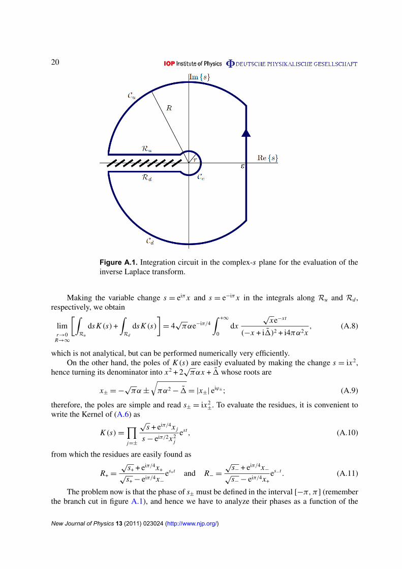
where we have used the ‘strong confinement’ form of the correlation transform (A.3), and ε > 0must be chosen so that all the poles of A (s + i1) stay to the left of the Re{s} = ε line. Themultivaluated character of

√s forces us to define a branch cut in the complex-s space; we chose

to remove the branch arg{s} = π , hence defining the phase of s in the domain [−π, π]. Then,choosing the integration contour as that in figure A.1, we can write the needed integral as∫ ε+i∞

ε−i∞dsK (s)= 2π i

∑j

R j − limr→0

R→∞

[∫Ru

dsK (s)+∫Rd

dsK (s)

], (A.7)

with R j being the residues of the kernel K (s)= A (s + i1) exp(st) at its poles [33]. Theintegrals over the paths Cu , Cd and Cc are zero when r → 0 and R → ∞.

8 We define the Laplace transform of a function f (t) as [33]

f (s)= Ls [ f (t)] =

∫ +∞

0dt e−st f (t), (A.1)

which satisfies the properties [33]

Ls[ f (t)] = s f (s)− f (0) and Ls

[∫ t

0dt ′ g

(t − t ′

)f(t ′)]

= g (s) f (s). (A.2)

New Journal of Physics 13 (2011) 023024 (http://www.njp.org/)

20

Figure A.1. Integration circuit in the complex-s plane for the evaluation of theinverse Laplace transform.

Making the variable change s = eiπ x and s = e−iπ x in the integrals along Ru and Rd ,respectively, we obtain

limr→0

R→∞

[∫Ru

dsK (s)+∫Rd

dsK (s)

]= 4

√παe−iπ/4

∫ +∞

0dx

√xe−xt

(−x + i1)2 + i4πα2x, (A.8)

which is not analytical, but can be performed numerically very efficiently.On the other hand, the poles of K (s) are easily evaluated by making the change s = ix2,

hence turning its denominator into x2 + 2√παx + 1 whose roots are

x± = −√πα±

√πα2 − 1= |x±| eiϕ±; (A.9)

therefore, the poles are simple and read s± = ix2±

. To evaluate the residues, it is convenient towrite the Kernel of (A.6) as

K (s)=

∏j=±

√s + eiπ/4x j

s − eiπ/2x2j

est , (A.10)

from which the residues are easily found as

R+ =

√s+ + eiπ/4x+

√s+ − eiπ/4x−

es+t and R− =

√s− + eiπ/4x−

√s− − eiπ/4x+

es−t . (A.11)

The problem now is that the phase of s± must be defined in the interval [−π, π] (rememberthe branch cut in figure A.1), and hence we have to analyze their phases as a function of the

New Journal of Physics 13 (2011) 023024 (http://www.njp.org/)

21

phases of x±, which we take in the interval [0, 2π ] as a convention. In terms of the parameters1 and α, we can define three regions:

• In the region 1 < 0 we have ϕ+ = 0 and ϕ− = π . Hence, we have to write

s+ = eiπ/2|x+|

2 and s− = eiπ/2|x−|

2 e2iπ× e−2iπ

; (A.12)

that is, we have to decrease the phase of s− by 2π to keep it within the interval [−π, π];with s± written in this way, the residues read

R+ =2 |x+|

|x+| + |x−|eix2

+t and R− = 0. (A.13)

• In the region 0< 1 < πα2, we have ϕ± = π , and hence, we have to decrease the phase ofboth s± by 2π to keep them within the interval [−π, π]; therefore both residues are zero,R± = 0.

• In the region 1 > πα2, we have ϕ+ ∈ [π/2, π] and ϕ− = [π, 3π/2]. Hence, we need towrite

s± = eiπ/2|x±|

2 e2iϕ± × e−2iπ and s− = eiπ/2|x−|

2 e2iϕ− × e−4iπ; (A.14)

that is, we decrease the phase of s+ by 2π and the phase of s− by 4π so that they both stayin the interval [−π, π], and then obtain

R+ = 0 and R− =2x−

x−x+eix2

−t . (A.15)

Introducing these results for the residues and the integral (A.8) in (A.7), we arrive at theexpression that we wanted to prove for the population A(t) (see (9)).

A.2. Steady-state population in the general case

From the last discussion, it should be clear that the long-term population is dictated solely bythe residues of K (s)= A (s + i1) exp(st). Moreover, only the residues corresponding to pureimaginary poles will remain in the t → ∞ limit, and hence the steady-state population will begiven by

|A (t → ∞)|2 =

∣∣∣∣∣∣∑

s j/Re{s j}=0

R j

∣∣∣∣∣∣2

. (A.16)

Then, to know the steady-state population in the finite trap case, we just need to find thepure imaginary poles of K (s) with the transform of the correlation function given by (A.2). Bywriting s = ix with x ∈ R, this amounts to solving the equation

x + 1+ 4�2 exp

(2x

ω0

)√2πx

ω30

[1 − erf

(√2x

ω0

)]= 0. (A.17)

This equation cannot be solved analytically, but it can be efficiently solved numerically.On the other hand, once we know the solutions x j of this equation, we can use them to evaluatetheir associated residues as [33]

R j =

{eix j t

d

ds[s + i1+ G (s + i1)]s=ix j

}−1

. (A.18)

This is the method that we have used to compute the results shown in figure 2(d).

New Journal of Physics 13 (2011) 023024 (http://www.njp.org/)

22

Appendix B. Evaluation of the Markov couplings (13)

In this appendix, we show that in the strong confinement regime, the Markov couplings have theform (13). After the Born–Markov approximation is carried out, the effective coupling betweendifferent sites has the form9

0j−l =

∫∞

0dτ Gj−l (τ )= lim

ε→0+

∑k

g2k

h2

exp[i (k − kL) · rj−l

]ε + i1k

. (B.1)

In the limit kL � X−10 (in which we can remove kL from gk; see (4)), taking the continuous limit

for the momentum, and performing the angular part of the integral over momenta by assumingthat rj−l is within the z-axis, this expression can be reduced to

0j−l =8X0�

2

iπ 1/2ω0e−ikL·rj−l

[∫∞

0dk sinc(krj−l) exp(−X 2

0k2)

− limε→0+

(1+ iε)∫

∞

0dk

sinc(krj−l) exp(−X 20k2)

1+ iε− (hk2/2m)

]. (B.2)

The first integral is easily evaluated as∫∞

0dk sinc(krj−l) exp

(−X 2

0k2)=

π

2rj−lerf

(rj−l

2X0

). (B.3)

The second integral is not analytical in general. Nevertheless, in the strong confinement regime,both |1|/ω0 and X0/d0 are small, and hence the Gaussian function in the Kernel can beapproximated by one, so that the remaining integral reads∫

∞

0dk

sinc(krj−l)

1+ iε−hk2

2m

=π

2rj−l(1+ iε)

1 − exp

irj−l

X0

√2(1+ iε)

ω0

. (B.4)

Introducing these integrals in (B.2) and taking the ε→ 0 limit, we arrive at expression (13) forthe Markov couplings.

References

[1] Jaksch D and Zoller P 2004 The cold atom Hubbard toolbox Ann. Phys. 315 52–79[2] Lewenstein M, Sanpera A, Ahufinger V, Damski B, Send(De) A and Sen U 2007 Ultracold atomic gases in

optical lattices: mimicking condensed matter physics and beyond Adv. Phys. 56 243–379[3] Bloch I, Dalibard J and Zwerger W 2008 Many-body physics with ultracold gases Rev. Mod. Phys. 80 885[4] Jaksch D, Bruder C, Cirac J I, Gardiner C W and Zoller P 1998 Cold bosonic atoms in optical lattices

Phys. Rev. Lett. 81 3108[5] Greiner M, Mandel O, Esslinger T, Hänsch T W and Bloch I 2002 Quantum phase transition from a superfluid

to a Mott insulator in a gas of ultracold atoms Nature 415 39–44[6] Schneider U, Hackermüller L, Will S, Best Th., Bloch I, Costi T A, Helmes R W, Rasch D and Rosch A 2008

Metallic and insulating phases of repulsively interacting fermions in a 3D optical lattice Science 322 1520

9 Note that ε is more than just a mathematical artefact for regularizing the integral. It accounts for the decoherencechannels not taken into account in the model, which make the correlation between lattice sites decay asGj−l(τ )exp(−ετ). Even if these channels appear at a time scale larger than the relevant times (ε� 1), they removethe zeros of the kernel’s denominator, showing that its singularities are not physical.

New Journal of Physics 13 (2011) 023024 (http://www.njp.org/)

23

[7] Hadzibabic Z, Krüger P, Cheneau M, Battelier B and Dalibard J 2006 Berezinskii–Kosterlitz–Thoulesscrossover in a trapped atomic gas Nature 441 1118–21

[8] Anderlini M, Lee P J, Brown B L, Sebby-Strabley J, Phillips W D and Porto J V 2007 Controlled exchangeinteraction between pairs of neutral atoms in an optical lattice Nature 448 452–6

[9] de Vega I, Porras D and Ignacio Cirac J 2008 Matter-wave emission in optical lattices: single particle andcollective effects Phys. Rev. Lett. 101 260404

[10] Dicke R H 1954 Coherence in spontaneous radiation processes Phys. Rev. 93 99[11] Gross M and Haroche S 1982 Superradiance: an essay on the theory of collective spontaneous emission

Phys. Rep. 93 301–96[12] Ernst V and Stehle P 1968 Emission of radiation from a system of many excited atoms Phys. Rev. 176 1456–79[13] Agarwal G S 1970 Master-equation approach to spontaneous emission Phys. Rev. A 2 2038–46[14] Rehler N E and Eberly J H 1971 Superradiance Phys. Rev. A 3 1735–51[15] Eberly J H 2006 Emission of one photon in an electric dipole transition of one among N atoms J. Phys. B:

Atom. Mol. Opt. Phys. 39 S599[16] Scully M O, Fry E S, Raymond Ooi C H and Wódkiewicz K 2006 Directed spontaneous emission from an

extended ensemble of N atoms: timing is everything Phys. Rev. Lett. 96 010501[17] Porras D and Cirac J I 2007 Quantum engineering of photon states with entangled atomic ensembles

arXiv:0704.0641[18] Porras D and Cirac J I 2008 Collective generation of quantum states of light by entangled atoms Phys. Rev. A

78 053816[19] Scully M O 2009 Collective Lamb shift in single photon Dicke superradiance Phys. Rev. Lett. 102 143601[20] Scully M O and Svidzinsky A A 2009 The super of superradiance Science 325 1510–1[21] John S and Quang T 1994 Spontaneous emission near the edge of a photonic band gap Phys. Rev. A 50 1764–9[22] John S and Quang T 1995 Localization of superradiance near a photonic band gap Phys. Rev. Lett. 74 3419–22[23] John S 1984 Electromagnetic absorption in a disordered medium near a photon mobility edge Phys. Rev. Lett.

53 2169–72[24] Chin C, Grimm R, Julienne P and Tiesinga E 2010 Feshbach resonances in ultracold gases Rev. Mod. Phys.

82 1225–86[25] Paredes B, Widera A, Murg V, Mandel O, Folling S, Cirac I, Shlyapnikov G V, Hänsch T W and Bloch I 2004

Tonks–Girardeau gas of ultracold atoms in an optical lattice Nature 429 277–81[26] Greiner W and Reinhardt J 1996 Field Quantization (Berlin: Springer)[27] Weisskopf V F and Wigner E 1930 Berechnung der natürlichen linienbreite auf grund der diracschen

lichttheorie Z. Phys. 63 54[28] Scully M O and Suhail Zubairy M 1997 Quantum Optics (Cambridge: Cambridge University Press)[29] Breuer H-P and Petruccione F 2002 The Theory of Open Quantum Systems (Oxford: Oxford University Press)[30] Rousseau V G, Batrouni G G, Sheehy D E, Moreno J and Jarrell M 2010 Pure Mott phases in confined

ultracold atomic systems Phys. Rev. Lett. 104 167201[31] Friedberg R, Hartmann S R and Manassah J T 1972 Limited superradiant damping of small samples

Phys. Lett. A 40 365–6[32] Friedberg R and Hartmann S R 1974 Temporal evolution of superradiance in a small sphere Phys. Rev. A

10 1728–39[33] Riley K F, Hobson M P and Bence S J 2006 Mathematical Methods for Physics and Engineering (Cambridge:

Cambridge University Press)

New Journal of Physics 13 (2011) 023024 (http://www.njp.org/)