Simpson's paradox in psychological science: a practical guide

HYPOTHESIS AND THEORY ARTICLEpublished: 12 August 2013

doi: 10.3389/fpsyg.2013.00513

Simpson’s paradox in psychological science: a practicalguideRogier A. Kievit1,2*, Willem E. Frankenhuis3, Lourens J. Waldorp1 and Denny Borsboom1

1 Department of Psychological Methods, University of Amsterdam, Amsterdam, Netherlands2 Medical Research Council – Cognition and Brain Sciences Unit, Cambridge, UK3 Department of Developmental Psychology, Radboud University Nijmegen, Nijmegen, Netherlands

Edited by:

Joshua A. McGrane, The Universityof Western Australia, Australia

Reviewed by:

Mike W. L. Cheung, NationalUniversity of Singapore, SingaporeRink Hoekstra, University ofGroningen, Netherlands

*Correspondence:

Rogier A. Kievit, Medical ResearchCouncil - Cognition and BrainSciences Unit, 15 Chaucer Rd,Cambridge, CB2 7EF,Cambridgeshire, UKe-mail: [email protected]

The direction of an association at the population-level may be reversed within thesubgroups comprising that population—a striking observation called Simpson’s paradox.When facing this pattern, psychologists often view it as anomalous. Here, we arguethat Simpson’s paradox is more common than conventionally thought, and typicallyresults in incorrect interpretations—potentially with harmful consequences. We supportthis claim by reviewing results from cognitive neuroscience, behavior genetics, clinicalpsychology, personality psychology, educational psychology, intelligence research, andsimulation studies. We show that Simpson’s paradox is most likely to occur wheninferences are drawn across different levels of explanation (e.g., from populations tosubgroups, or subgroups to individuals). We propose a set of statistical markers indicativeof the paradox, and offer psychometric solutions for dealing with the paradox whenencountered—including a toolbox in R for detecting Simpson’s paradox. We show thatexplicit modeling of situations in which the paradox might occur not only prevents incorrectinterpretations of data, but also results in a deeper understanding of what data tell usabout the world.

Keywords: paradox, measurement, reductionism, Simpson’s paradox, statistical inference, ecological fallacy

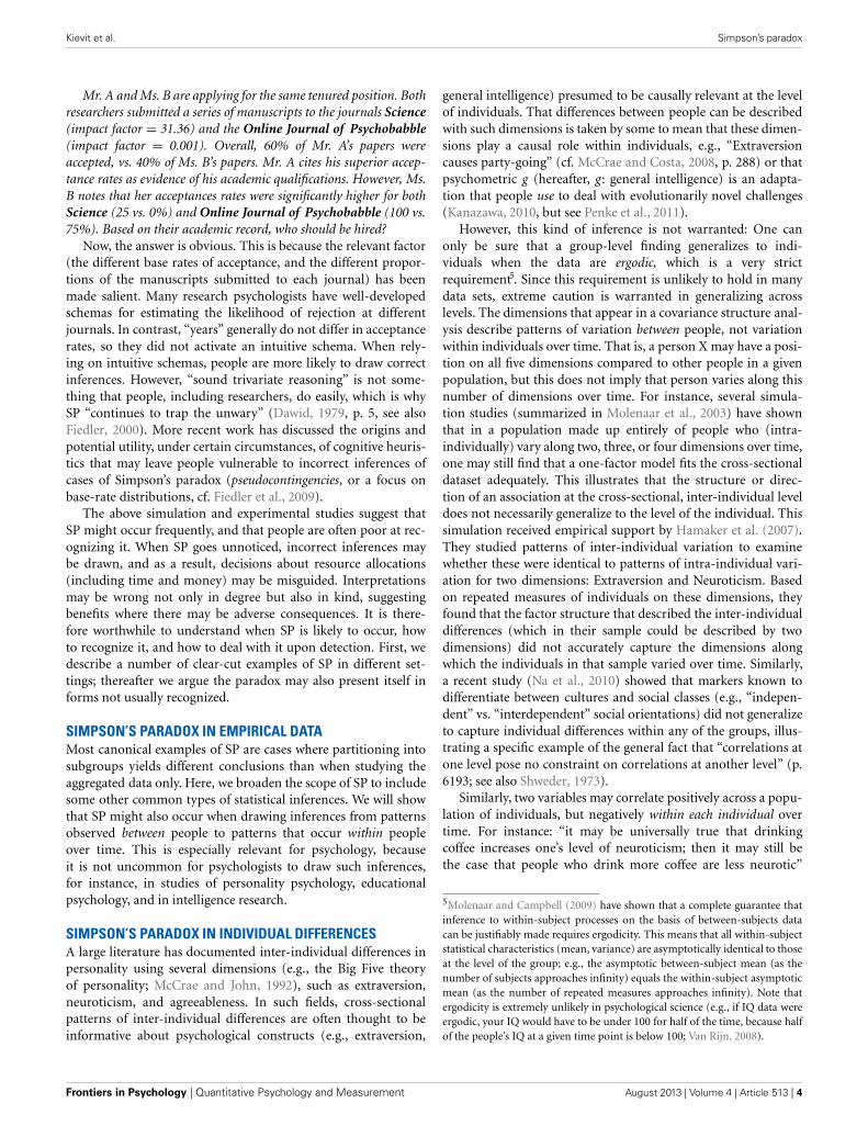
INTRODUCTIONTwo researchers, Mr. A and Ms. B, are applying for the sametenured position. Both researchers submitted a number ofmanuscripts to academic journals in 2010 and 2011: 60% of Mr.A’s papers were accepted, vs. 40% of Ms. B’s papers. Mr. A citeshis superior acceptance rate as evidence of his academic qualifica-tions. However, Ms. B notes that her acceptance rates were higherin both 2010 (25 vs. 0%) and 2011 (100 vs. 75%)1. Based on theserecords, who should be hired?2

In Simpson (1951) showed that a statistical relationshipobserved in a population—i.e., a collection of subgroups orindividuals—could be reversed within all of the subgroups thatmake up that population 3. This apparent paradox has signifi-cant implications for the medical and social sciences: A treatmentthat appears effective at the population-level may, in fact, haveadverse consequences within each of the population’s subgroups.For instance, a higher dosage of medicine may be associated with

1

2010 2011 overall

Mr. A 0 of 20 60 of 80 60%

Ms. B 20 of 80 20 of 20 40%

2The years in this example are substitutes for the true relevant variable,namely journal quality (together with diverging base rates of submission).This variable is substituted here to emphasize the puzzling nature of theparadox. See page 3 for further explanation of this (hypothetical) example.3The same observation was made, albeit less explicitly, by Pearson et al.(1899), Yule (1903) and Cohen and Nagel (1934); see also Aldrich (1995).

higher recovery rates at the population-level; however, withinsubgroups (e.g., for both males and females), a higher dosagemay actually result in lower recovery rates. Figure 1 illustratesthis situation: Even though a negative relationship exists between“Treatment Dosage” and “Recovery” in both males and females,when these groups are combined a positive trend appears (black,dashed). Thus, if analyzed globally, these data would suggest thata higher dosage treatment is preferable, while the exact oppo-site is true (the continuous case is often referred to as Robinson’sparadox, 1950)4.

Simpson’s paradox (hereafter SP) has been formally analyzedby mathematicians and statisticians (e.g., Blyth, 1972; Dawid,1979; Pearl, 1999, 2000; Schield, 1999; Tu et al., 2008; Greenland,2010; Hernán et al., 2011), its relevance for human inferencesstudied by psychologists (e.g., Schaller, 1992; Spellman, 1996a,b;Fiedler, 2000, 2008; Curley and Browne, 2001) and conceptu-ally explored by philosophers (e.g., Cartwright, 1979; Otte, 1985;Bandyoapdhyay et al., 2011). However, few works have discussedthe practical aspects of SP for empirical science: How mightresearchers prevent the paradox, recognize it, and deal with itupon detection? These issues are the focus of the present paper.

4Julious and Mullee (1994) showed such a pattern in a data set bearing ontreatment of kidney stones: Treatment A seemed more effective than treatmentB in the dataset as a whole, but when split into small and large kidney stones(which, combined, formed the entire data set), treatment B was more effectivefor both.

www.frontiersin.org August 2013 | Volume 4 | Article 513 | 1

Kievit et al. Simpson’s paradox

FIGURE 1 | Example of Simpson’s Paradox. Despite the fact that thereexists a negative relationship between dosage and recovery in both malesand females, when grouped together, there exists a positive relationship.All figures created using ggplot2 (Wickham, 2009). Data in arbitrary units.

Here, we argue that (a) SP occurs more frequently than com-monly thought, and (b) inadequate attention to SP results inincorrect inferences that may compromise not only the questfor truth, but may also jeopardize public health and policy. Weexamine the relevance of SP in several steps. First, we describeSP, investigate how likely it is to occur, and discuss work show-ing that people are not adept at recognizing it. Next, we reviewexamples drawn from a range of psychological fields, to illus-trate the circumstances, types of design and analyses that areparticularly vulnerable to instances of the paradox. Based on thisanalysis, we specify the circumstances in which SP is likely tooccur, and identify a set of statistical markers that aid in its iden-tification. Finally, we will provide countermeasures, aimed at theprevention, diagnosis, and treatment of SP—including a softwarepackage in the free statistical environment R (Team, 2013) createdto help researchers detect SP when testing bivariate relationships.

WHAT IS SIMPSON’S PARADOX?Strictly speaking, SP is not actually a paradox, but a counterintu-itive feature of aggregated data, which may arise when (causal)inferences are drawn across different explanatory levels: frompopulations to subgroups, or subgroups to individuals, or fromcross-sectional data to intra-individual changes over time (cf.Kievit et al., 2011). One of the canonical examples of SP concernspossible gender bias in admissions into Berkeley graduate school(Bickel et al., 1975; see also Waldmann and Hagmayer, 1995).Table 1 shows stylized admission statistics for males and femalesin two faculties (A and B) that together constitute the Berkeleygraduate program.

Overall, proportionally fewer females than males were admit-ted into graduate school (84% males vs. 78% females). However,when the admission proportions are inspected for the individ-ual graduate schools A and B, the reverse pattern holds: In bothschool A and B the proportion of females admitted is greater thanthat of males (97 vs. 91% in school A, and 33 vs. 20% percentin school B). This seems paradoxical: Globally, there appears to

be bias toward males, but when individual graduate schools aretaken into account, there seems to be bias toward females. Thisconflicts with our implicit causal interpretation of the aggregatedata, which is that the proportions of the aggregate data (84%males and 78% females) are informative about the relative like-lihoods of male or female applicants being admitted if they wereto apply to a Berkeley graduate school. In this example, SP arisesbecause of different proportions of males and females attempt toenter schools that differ in their thresholds for accepting students;we discuss this explanation in more detail later.

Pearl (1999) notes that SP is unsurprising: “seeing magnitudeschange upon conditionalization is commonplace, and seeing suchchanges turn into sign reversal (. . . ) is not uncommon either”(p. 3). However, although mathematically trivial, sign reversalsare crucial for science and policy. For example, a (small) posi-tive effect of a drug on recovery, or an educational reform onlearning performance, provides incentives for further research,investment of resources, and implementation. By contrast, a neg-ative effect may warrant recall of a drug, cessation of researchefforts and (when discovered after implementation) could gener-ate very serious ethical concerns. Although the difference betweena positive effect of d = 0.5 and d = 0.9 may be considered largerin statistical terms than the difference between, say, d = 0.15and d = −0.15, the latter might entail a more critical difference:Decisions based on the former are wrong in degree, but thosebased on the latter in kind. This can create major potential forharm and omission of benefit. Simpson’s paradox is conceptuallyand analytically related to many statistical challenges and tech-niques, including causal inference (Pearl, 2000, 2013), the eco-logical fallacy (Robinson, 1950; Kramer, 1983; King, 1997; Kingand Roberts, 2012), Lord’s paradox, (Tu et al., 2008), propensityscore matching (Rosenbaum and Rubin, 1983), suppressor vari-ables (Conger, 1974; Tu et al., 2008), conditional independence(Dawid, 1979), partial correlations (Fisher, 1925), p-technique(Cattell, 1952) and mediator variables (MacKinnon et al., 2007).The underlying shared theme of these techniques is that theyare concerned with the nature of (causal) inference: The chal-lenge is what inferences are warranted based on the data weobserve. According to Pearl (1999), it is exactly our tendency toautomatically interpret observed associations causally that ren-ders SP paradoxical. For instance, in the Berkeley admissionsexample, many might incorrectly interpret the data in the fol-lowing way: “The data show that if male and female studentsapply to Berkeley graduate school, females are less likely to beaccepted.” A careful consideration of the reversals of conditionalprobabilities within the graduate schools guards us against thisinitial false inference by illustrating that this pattern need nothold within graduate schools. Of course this first step does notfully resolve the issue: Even though the realization that the condi-tional acceptance rates are reversed within every graduate schoolshas increased our insight into the possible true underlying pat-terns, these acceptance rates are still compatible, under variousassumptions, with various causal mechanisms (including bothbias against women or men). This is important, as it is thesecausal mechanisms that are the main payoff of empirical research.However, to be able to draw causal conclusions, we must knowwhat the underlying causal mechanisms of the observed patterns

Frontiers in Psychology | Quantitative Psychology and Measurement August 2013 | Volume 4 | Article 513 | 2

Kievit et al. Simpson’s paradox

Table 1 | A stylized representation of Berkeley admission statistics.

Male Female Proportion males Proportion females Summary

Accept Reject Accept Reject

Faculty A 820 80 680 20 0.91 0.97 More females

Faculty B 20 80 100 200 0.2 0.33 More females

Combined 840 160 780 220 0.84 0.78 More males

Total N 1000 1000

The counts in each cell reflect students in each category, accepted or rejected, for two graduate schools. The numbers are fictitious, designed to emphasize the key

points.

are, and to what extent the data we observe are informative aboutthese mechanisms.

SIMPSON’S PARADOX IN REAL LIFEDespite the fact that SP has been repeatedly recognized in datasets, documented cases are often treated as noteworthy excep-tions (e.g., Bickel et al., 1975; Scheiner et al., 2000; Chuanget al., 2009). This is most clearly reflected in one paper’sprovocative title: “Simpson’s Paradox in Real Life” (Wagner,1982). However, there are reasons to doubt the default assump-tion that SP is a rare curiosity. In psychology, SP has beenrecognized in a wide range of domains, including the studyof memory (Hintzman, 1980, 1993), decision making (Curleyand Browne, 2001), strategies in prisoners dilemma games(Chater et al., 2008), tracking of changes in educational per-formance changes over time (Wainer, 1986), response strategies(van der Linden et al., 2011), psychopathological comorbid-ity (Kraemer et al., 2006), victim-offender overlap (Reid andSullivan, 2012), the use of antipsychotics for dementia (Suh,2009), and even meta-analyses (Rücker and Schumacher, 2008;Rubin, 2011).

A recent simulation study by Pavlides and Perlman (2009) sug-gests SP may occur more often than commonly thought. Theyquantified the likelihood of SP in simulated data by examininga range of 2 × 2 × 2 tables for uniformly distributed randomdata. For the simple 2 × 2 × 2 case, a full sign reversal—whereboth complementary subpopulations show a sign opposite totheir aggregate—occurred in 1.67% of the simulated cases.Although much depends on the exact specifications of thedata, this number should be a cause of concern: This sim-ulation suggests SP might occur in nearly 2% of compara-ble datasets, but reports of SP in empirical data are far lesscommon.

Simulation studies cannot be used, in isolation, to esti-mate the prevalence of SP in the published literature, giventhat there are several plausible mechanisms by which the pub-lished literature might overestimate (empirical instances of SPare interesting, and therefore likely to be published) or under-estimate (datasets with cases of SP may yield ambiguous orconflicting answers, possibly inducing file-drawer type effects)the true prevalence of SP. Unfortunately, a (hypothetical) re-analysis of raw data in the published literature to estimate the“true” prevalence of SP would suffer from similar problems:Previous work has shown that the probability of data-sharing is

not unrelated to the nature of the data (e.g., see Wicherts et al.,2006, 2011).

Still, there are good reasons to think SP might occur moreoften than it is reported in the literature, including the fact thatpeople are not necessarily very adept at detecting the paradoxwhen observing it. Fiedler et al. (2003) provided participantswith several scenarios similar to the sex discrimination examplepresented in Table 1: Fewer females were admitted to fictionalUniversity X; however, within each of two graduate schoolsUniversity X’s admission rates for females were higher. This signreversal was caused by a difference in base rates, with morefemales applying to the more selective graduate school. Fiedlerand colleagues showed that it was very difficult to have peo-ple engage in “sound trivariate reasoning” (p. 16): Participantsfailed to recognize the paradox, even when they were explicitlyprimed. In five experiments, they made all relevant factors salientin varying degrees of explicitness. For instance, the difference inadmission base rates of two universities would be explicit (“Thesetwo universities differ markedly in their application standards”)as well as the sex difference in applying for the difficult school(“women are striving for ambitious goals”). After such primes,participants correctly identified: (1) the difference in graduateschools admission rates, (2) the sex difference in application ratesto both schools and even (3) the relative success of males andfemales within both schools. Nonetheless, they still drew incor-rect conclusions, basing their assessment solely on the aggregatedata (i.e., “women were discriminated against”). The authorsconclude: “Within the present task setting, then, there is little evi-dence for a mastery of Simpson’s paradox that goes beyond themost primitive level of undifferentiated guessing” (p. 21).

However, other studies suggest that in certain settings sub-jects do take into account conditional contingencies in order tojudge the causal efficacy of the fertilizer (Spellman, 1996a,b). Inan extension of these findings, Spellman et al. (2001) showed thatthe extent to which people took into account conditional prob-abilities appropriately depended on the activation of top-downvs. bottom-up mental models of interacting causes. In a series ofexperiments where participants had to judge the effectiveness ofa type of fertilizer, people were able to estimate the correct rateswhen primed by a visual cue representing the underlying causalfactor. To demonstrate the force of such top-down schemas, letus revisit our initial example, of Mr. A and Ms. B, presentedin a slightly modified fashion (but with identical numbers, seeFootnote 1):

www.frontiersin.org August 2013 | Volume 4 | Article 513 | 3

Kievit et al. Simpson’s paradox

Mr. A and Ms. B are applying for the same tenured position. Bothresearchers submitted a series of manuscripts to the journals Science(impact factor = 31.36) and the Online Journal of Psychobabble(impact factor = 0.001). Overall, 60% of Mr. A’s papers wereaccepted, vs. 40% of Ms. B’s papers. Mr. A cites his superior accep-tance rates as evidence of his academic qualifications. However, Ms.B notes that her acceptances rates were significantly higher for bothScience (25 vs. 0%) and Online Journal of Psychobabble (100 vs.75%). Based on their academic record, who should be hired?

Now, the answer is obvious. This is because the relevant factor(the different base rates of acceptance, and the different propor-tions of the manuscripts submitted to each journal) has beenmade salient. Many research psychologists have well-developedschemas for estimating the likelihood of rejection at differentjournals. In contrast, “years” generally do not differ in acceptancerates, so they did not activate an intuitive schema. When rely-ing on intuitive schemas, people are more likely to draw correctinferences. However, “sound trivariate reasoning” is not some-thing that people, including researchers, do easily, which is whySP “continues to trap the unwary” (Dawid, 1979, p. 5, see alsoFiedler, 2000). More recent work has discussed the origins andpotential utility, under certain circumstances, of cognitive heuris-tics that may leave people vulnerable to incorrect inferences ofcases of Simpson’s paradox (pseudocontingencies, or a focus onbase-rate distributions, cf. Fiedler et al., 2009).

The above simulation and experimental studies suggest thatSP might occur frequently, and that people are often poor at rec-ognizing it. When SP goes unnoticed, incorrect inferences maybe drawn, and as a result, decisions about resource allocations(including time and money) may be misguided. Interpretationsmay be wrong not only in degree but also in kind, suggestingbenefits where there may be adverse consequences. It is there-fore worthwhile to understand when SP is likely to occur, howto recognize it, and how to deal with it upon detection. First, wedescribe a number of clear-cut examples of SP in different set-tings; thereafter we argue the paradox may also present itself informs not usually recognized.

SIMPSON’S PARADOX IN EMPIRICAL DATAMost canonical examples of SP are cases where partitioning intosubgroups yields different conclusions than when studying theaggregated data only. Here, we broaden the scope of SP to includesome other common types of statistical inferences. We will showthat SP might also occur when drawing inferences from patternsobserved between people to patterns that occur within peopleover time. This is especially relevant for psychology, becauseit is not uncommon for psychologists to draw such inferences,for instance, in studies of personality psychology, educationalpsychology, and in intelligence research.

SIMPSON’S PARADOX IN INDIVIDUAL DIFFERENCESA large literature has documented inter-individual differences inpersonality using several dimensions (e.g., the Big Five theoryof personality; McCrae and John, 1992), such as extraversion,neuroticism, and agreeableness. In such fields, cross-sectionalpatterns of inter-individual differences are often thought to beinformative about psychological constructs (e.g., extraversion,

general intelligence) presumed to be causally relevant at the levelof individuals. That differences between people can be describedwith such dimensions is taken by some to mean that these dimen-sions play a causal role within individuals, e.g., “Extraversioncauses party-going” (cf. McCrae and Costa, 2008, p. 288) or thatpsychometric g (hereafter, g: general intelligence) is an adapta-tion that people use to deal with evolutionarily novel challenges(Kanazawa, 2010, but see Penke et al., 2011).

However, this kind of inference is not warranted: One canonly be sure that a group-level finding generalizes to indi-viduals when the data are ergodic, which is a very strictrequirement5. Since this requirement is unlikely to hold in manydata sets, extreme caution is warranted in generalizing acrosslevels. The dimensions that appear in a covariance structure anal-ysis describe patterns of variation between people, not variationwithin individuals over time. That is, a person X may have a posi-tion on all five dimensions compared to other people in a givenpopulation, but this does not imply that person varies along thisnumber of dimensions over time. For instance, several simula-tion studies (summarized in Molenaar et al., 2003) have shownthat in a population made up entirely of people who (intra-individually) vary along two, three, or four dimensions over time,one may still find that a one-factor model fits the cross-sectionaldataset adequately. This illustrates that the structure or direc-tion of an association at the cross-sectional, inter-individual leveldoes not necessarily generalize to the level of the individual. Thissimulation received empirical support by Hamaker et al. (2007).They studied patterns of inter-individual variation to examinewhether these were identical to patterns of intra-individual vari-ation for two dimensions: Extraversion and Neuroticism. Basedon repeated measures of individuals on these dimensions, theyfound that the factor structure that described the inter-individualdifferences (which in their sample could be described by twodimensions) did not accurately capture the dimensions alongwhich the individuals in that sample varied over time. Similarly,a recent study (Na et al., 2010) showed that markers known todifferentiate between cultures and social classes (e.g., “indepen-dent” vs. “interdependent” social orientations) did not generalizeto capture individual differences within any of the groups, illus-trating a specific example of the general fact that “correlations atone level pose no constraint on correlations at another level” (p.6193; see also Shweder, 1973).

Similarly, two variables may correlate positively across a popu-lation of individuals, but negatively within each individual overtime. For instance: “it may be universally true that drinkingcoffee increases one’s level of neuroticism; then it may still bethe case that people who drink more coffee are less neurotic”

5Molenaar and Campbell (2009) have shown that a complete guarantee thatinference to within-subject processes on the basis of between-subjects datacan be justifiably made requires ergodicity. This means that all within-subjectstatistical characteristics (mean, variance) are asymptotically identical to thoseat the level of the group; e.g., the asymptotic between-subject mean (as thenumber of subjects approaches infinity) equals the within-subject asymptoticmean (as the number of repeated measures approaches infinity). Note thatergodicity is extremely unlikely in psychological science (e.g., if IQ data wereergodic, your IQ would have to be under 100 for half of the time, because halfof the people’s IQ at a given time point is below 100; Van Rijn, 2008).

Frontiers in Psychology | Quantitative Psychology and Measurement August 2013 | Volume 4 | Article 513 | 4

Kievit et al. Simpson’s paradox

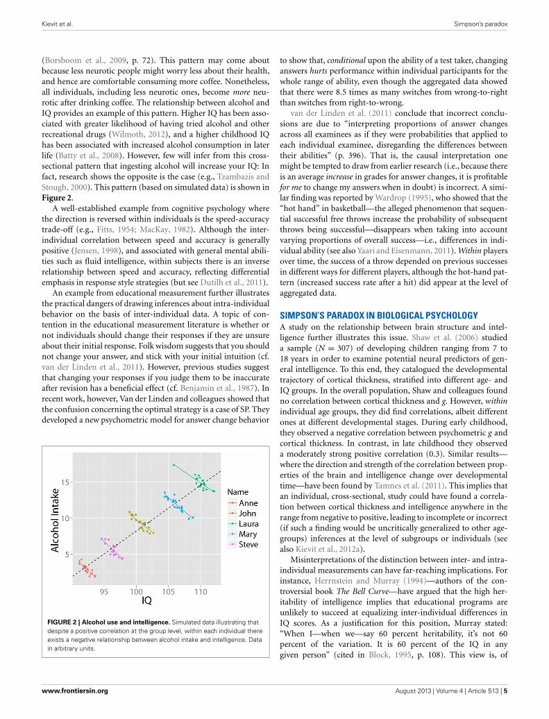
(Borsboom et al., 2009, p. 72). This pattern may come aboutbecause less neurotic people might worry less about their health,and hence are comfortable consuming more coffee. Nonetheless,all individuals, including less neurotic ones, become more neu-rotic after drinking coffee. The relationship between alcohol andIQ provides an example of this pattern. Higher IQ has been asso-ciated with greater likelihood of having tried alcohol and otherrecreational drugs (Wilmoth, 2012), and a higher childhood IQhas been associated with increased alcohol consumption in laterlife (Batty et al., 2008). However, few will infer from this cross-sectional pattern that ingesting alcohol will increase your IQ: Infact, research shows the opposite is the case (e.g., Tzambazis andStough, 2000). This pattern (based on simulated data) is shown inFigure 2.

A well-established example from cognitive psychology wherethe direction is reversed within individuals is the speed-accuracytrade-off (e.g., Fitts, 1954; MacKay, 1982). Although the inter-individual correlation between speed and accuracy is generallypositive (Jensen, 1998), and associated with general mental abili-ties such as fluid intelligence, within subjects there is an inverserelationship between speed and accuracy, reflecting differentialemphasis in response style strategies (but see Dutilh et al., 2011).

An example from educational measurement further illustratesthe practical dangers of drawing inferences about intra-individualbehavior on the basis of inter-individual data. A topic of con-tention in the educational measurement literature is whether ornot individuals should change their responses if they are unsureabout their initial response. Folk wisdom suggests that you shouldnot change your answer, and stick with your initial intuition (cf.van der Linden et al., 2011). However, previous studies suggestthat changing your responses if you judge them to be inaccurateafter revision has a beneficial effect (cf. Benjamin et al., 1987). Inrecent work, however, Van der Linden and colleagues showed thatthe confusion concerning the optimal strategy is a case of SP. Theydeveloped a new psychometric model for answer change behavior

FIGURE 2 | Alcohol use and intelligence. Simulated data illustrating thatdespite a positive correlation at the group level, within each individual thereexists a negative relationship between alcohol intake and intelligence. Datain arbitrary units.

to show that, conditional upon the ability of a test taker, changinganswers hurts performance within individual participants for thewhole range of ability, even though the aggregated data showedthat there were 8.5 times as many switches from wrong-to-rightthan switches from right-to-wrong.

van der Linden et al. (2011) conclude that incorrect conclu-sions are due to “interpreting proportions of answer changesacross all examinees as if they were probabilities that applied toeach individual examinee, disregarding the differences betweentheir abilities” (p. 396). That is, the causal interpretation onemight be tempted to draw from earlier research (i.e., because thereis an average increase in grades for answer changes, it is profitablefor me to change my answers when in doubt) is incorrect. A simi-lar finding was reported by Wardrop (1995), who showed that the“hot hand” in basketball—the alleged phenomenon that sequen-tial successful free throws increase the probability of subsequentthrows being successful—disappears when taking into accountvarying proportions of overall success—i.e., differences in indi-vidual ability (see also Yaari and Eisenmann, 2011). Within playersover time, the success of a throw depended on previous successesin different ways for different players, although the hot-hand pat-tern (increased success rate after a hit) did appear at the level ofaggregated data.

SIMPSON’S PARADOX IN BIOLOGICAL PSYCHOLOGYA study on the relationship between brain structure and intel-ligence further illustrates this issue. Shaw et al. (2006) studieda sample (N = 307) of developing children ranging from 7 to18 years in order to examine potential neural predictors of gen-eral intelligence. To this end, they catalogued the developmentaltrajectory of cortical thickness, stratified into different age- andIQ groups. In the overall population, Shaw and colleagues foundno correlation between cortical thickness and g. However, withinindividual age groups, they did find correlations, albeit differentones at different developmental stages. During early childhood,they observed a negative correlation between psychometric g andcortical thickness. In contrast, in late childhood they observeda moderately strong positive correlation (0.3). Similar results—where the direction and strength of the correlation between prop-erties of the brain and intelligence change over developmentaltime—have been found by Tamnes et al. (2011). This implies thatan individual, cross-sectional, study could have found a correla-tion between cortical thickness and intelligence anywhere in therange from negative to positive, leading to incomplete or incorrect(if such a finding would be uncritically generalized to other age-groups) inferences at the level of subgroups or individuals (seealso Kievit et al., 2012a).

Misinterpretations of the distinction between inter- and intra-individual measurements can have far-reaching implications. Forinstance, Herrnstein and Murray (1994)—authors of the con-troversial book The Bell Curve—have argued that the high her-itability of intelligence implies that educational programs areunlikely to succeed at equalizing inter-individual differences inIQ scores. As a justification for this position, Murray stated:“When I—when we—say 60 percent heritability, it’s not 60percent of the variation. It is 60 percent of the IQ in anygiven person” (cited in Block, 1995, p. 108). This view is, of

www.frontiersin.org August 2013 | Volume 4 | Article 513 | 5

Kievit et al. Simpson’s paradox

course, incorrect, as heritability measures capture a pattern ofco-variation between individuals (for an excellent discussion ofanalyses of variance vs. analyses of causes, see Lewontin, 2006).Here too it is clear that inferences drawn across different levels ofexplanations (in this case, from between- to within-individuals)may go awry, and such incorrect inferences may affect policychanges (e.g., banning educational programs based on the invalidinference that individuals’ intelligences are fully fixed by theirgenomes).

A SURVIVAL GUIDE TO SIMPSON’S PARADOXWe have shown that SP may occur in a wide variety of researchdesigns, methods, and questions. As such, it would be useful todevelop means to “control” or minimize the risk of SP occur-ring, much like we wish to control instances of other statisticalproblems. Pearl (1999, 2000) has shown that (unfortunately)there is no single mathematical property that all instances of SPhave in common, and therefore, there will not be a single, cor-rect rule for analyzing data so as to prevent cases of SP. Basedon graphical models, Pearl (2000) shows that conditioning onsubgroups may sometimes be appropriate, but may sometimesincrease spurious dependencies (see also Spellman et al., 2001). Itappears that some cases are observationally equivalent, and onlywhen it can be assumed that the cause of interest does not influ-ence another variable associated with the effect, a test exists todetermine whether SP can arise (see Pearl, 2000, chapter 6 fordetails).

However, what we can do is consider the instances of SPwe are most likely to encounter, and investigate them for char-acteristic warning signals. Psychology is often concerned withthe average performance of groups of individuals (e.g., grad-uate students), and drawing valid inferences applying to thatentire group, including its subgroups (e.g., males and females).The above examples show how such inferences may go awry.Given the general structure of psychological studies, the oppo-site incorrect inference is much less likely to occur: very fewpsychological studies examine a single individual over a periodof time in the absence of aggregated data, to then infer fromthat individual a population level regularity. Thus, the incor-rect generalization from an individual to a group is less likely,both in terms of prevalence (there are fewer time-series thancross-sectional studies) and in terms of statistical inference (moststudies that collect time-series data—as Hamaker et al. (2007)did—are specifically designed to address complex statisticaldynamics).

The most general “danger” for psychology is therefore well-defined: We might incorrectly infer that a finding at the level ofthe group generalizes to subgroups, or to individuals over time.All examples we discussed above are of this kind. Although thereis no single, general solution even in this case, there are ways ofaddressing this most likely problem that often succeed. In thisspirit, the next section offers practical and diagnostic tools todeal with possible instances of SP. We discuss strategies for threephases of the research process: Prevention, diagnosis, and treat-ment of SP. Thus, the first section will concern data that has yetto be acquired, the latter two with data that has been collectedalready.

PREVENTING SIMPSON’S PARADOXDevelop and test mechanistic explanationsThe first step in addressing SP is to carefully consider when itmay arise. There is nothing inherently incorrect about the datareflected in puzzling contingency tables or scatterplots: Rather,the mechanistic inference we propose to explain the data may beincorrect. This danger arises when we use data at one explana-tory level to infer a cause at a different explanatory level. Considerthe example of alcohol use and IQ mentioned before. The cross-sectional finding that higher alcohol consumption correlates withhigher IQ is perfectly valid, and may be interesting for a varietyof sociological or cultural reasons (cf. Martin, 1981 for a similarpoint regarding the Berkeley admission statistics). Problems arisewhen we infer from this inter-individual pattern that an individ-ual might increase their IQ by drinking more alcohol (an intra-individual process). Of course in the case of alcohol and IQ, thereis little danger of making this incorrect inference because of strongtop-down knowledge constraining our hypotheses. But, as we sawin the example of scientist A and B, in the absence of top-downknowledge, we are far less well-protected against making incor-rect inferences. Without well-developed top-down schemas, wehave, in essence, a cognitive blind spot within which we are vul-nerable to making incorrect inferences. It is this blind spot that, inour view, is the source of consistent underestimation of the preva-lence of SP. A first step against guarding against this danger is byexplicitly proposing a mechanism, determining at which level it ispresumed to operate (between groups, within groups, within peo-ple), and then carefully assessing whether the explanatory level atwhich the data were collected aligns with the explanatory level ofthe proposed mechanism (see Kievit et al., 2012b). In this manner,we think many instances of SP can be avoided.

Study changeOne of the most neglected areas of psychology is the analy-sis of individual changes through time. Despite calls for moreattention for such research (e.g., Molenaar, 2004; Molenaar andCampbell, 2009), most psychological research uses snapshot mea-surements of groups of individuals, not repeated measures overtime. However, of course, intra-individual patterns can be stud-ied; such fields as medicine have a long tradition of doing so (e.g.,survival curve analysis). Moreover, many practical obstacles for“idiographic” psychology (e.g., logistic issues and costs associ-ated with asking participants to repeatedly visit the lab) can beovercome by using modern technological tools. For instance, theadvent of smartphone technology opens up a variety of meansto relatively non-invasively collect psychological data outside ofthe lab within the same individual over time (cf. Miller, 2012).Moreover, time-series data also allows for the study of aggregatepatterns.

InterveneIf we want to be sure the relationship between two variablesat the group level reflects a causal pattern within individualsover time, the most informative strategy is to experimentallyintervene within individuals. For instance, across individuals, wemight observe a positive correlation between high levels of testos-terone and aggressive behavior. This still leaves open multiple

Frontiers in Psychology | Quantitative Psychology and Measurement August 2013 | Volume 4 | Article 513 | 6

Kievit et al. Simpson’s paradox

possibilities; for instance, some people may be genetically predis-posed to have both higher levels of testosterone and aggressivebehavior, even though the two have no causal relationship. If so,despite the aggregate positive correlation within each individualover time, we would not observe a consistent relationship. Ofcourse, it may be the case that there does exist a stable, consistentpositive association within every individual between fluctuationsin testosterone and variations in aggressive behaviors. But eventhis pattern does not necessarily address the causal question: Dochanges in testosterone affect aggressive behavior?

To answer the causal question, we need to devise an exper-imental study: If we administer a dose of testosterone, doesaggressive behavior increase; and, conversely, if we induce aggres-sive behavior, do testosterone levels increase? As it turns out, theevidence suggests that both these patterns are supported (e.g.,Mazur and Booth, 1998). Note that the cross-sectional patternof a positive correlation between testosterone and aggression iscompatible (perhaps counter-intuitively) with all possible out-comes at the intra-individual level following an intervention,including a decrease in aggressive symptoms after an injectionwith testosterone within individuals. To model the effect of somemanipulation, and therefore rule out SP at the level of the individ-ual (i.e., a reversal of the direction of association), the strongestapproach is a study that can assess the effects of an intervention,preferably within individual subjects.

DIAGNOSIS OF SIMPSON’S PARADOXIf we already collected data and want to know whether our datamight contain an instance of SP, what we want to know is whethera certain statistical relationship at the group level is the same forall subgroups in which the data may defensibly be partitioned,which could be subgroups or individuals (in repeated measuresdesigns). Below we discuss various strategies to diagnose whetherthis is the case.

VISUALIZE THE DATAIn bivariate continuous data sets, the first step in diagnosinginstances of SP is to visualize the data. As the above figures (e.g.,Figures 1, 2) demonstrate, instances of SP can become appar-ent when data is plotted, even when nothing in our statisticalanalyses suggests SP exists in the data. Moreover, as the aboveexperiments have illustrated (e.g., Spellman, 1996a), under manycircumstances people are quite inept at inferring conditional rela-tionships based on summary statistics. Visual representations insuch cases may, in the memorable words of Loftus (1993), “beworth a thousand p values.” For these reasons, if a statistical testis performed, it should always be accompanied by visualization inorder to facilitate the interpretation of possible instance of SP.

Despite being a powerful tool for detecting SP, visualizationalone does not suffice. First, not all instances of SP are obviousfrom simple visual representations. Consider Figure 3A, whichvisualizes the relationship of data collected by a researcher study-ing the relationship between arousal and performance on someathletic skill such as, say, tennis. This figure would be what isavailable to a researcher on the basis of this bivariate dataset, andbased on a regression analysis, (s)he concludes that there is nosignificant association. However, imagine that the researcher now

FIGURE 3 | Visualization alone does not always suffice. (A) shows thebivariate relationship between arousal and performance of tennis players,suggesting no relationship. However, after collecting new data on playingstyles (e.g., how many winning shots, how many errors) we perform acluster analysis yielding two types of players (“aggressive” and“defensive”). By including this new, bivariate variable, two clear andopposite relationships (B) emerge that would have gone unnoticedotherwise.

gains access to a large body of (previously inaccessible) additionaldata on the game statistics of each player: How many winningshots do they make, how many errors, how often do they hitwith topspin or backspin, how hard do they hit the ball? Nowimagine that using this new data, (s)he performs a cluster (orother type of classification) analysis on these additional vari-ables, yielding two player types that we may label “aggressive” vs.“defensive”6. By including this additional (latent) grouping vari-able in our analysis, as can be seen in Figure 3B, we can see thevalue of latent clustering: In the aggressive players, there is a (sig-nificant) positive relationship between arousal and performance,whereas in the defensive players, there is a negative relationshipbetween arousal and performance (a special case of the Yerkes-Dodson law, e.g., Anderson et al., 1989). Later we discuss anempirical example that has such a structure (Reid and Sullivan,2012).

6E.g., a value such as the “aggressive margin” collected by MatchPro, http://mymatchpro.com/stats.html, defined as “(Winners + opponent’s forcederrors − unforced errors)/total points played.”

www.frontiersin.org August 2013 | Volume 4 | Article 513 | 7

Kievit et al. Simpson’s paradox

Second, not all data can be visualized in such a way that thepossibility of conditional reversals is obvious to practicing sci-entists. Bivariate continuous data are especially suited for thispurpose, but in other cases (such as contingency tables), the datacan be (a) difficult to visualize and (b) the experimental evidencediscussed above (e.g., Spellman, 1996a) in section “Simpson’sparadox in real life” suggests that, even when presented withall the data and specifically reminded to consider conditionalinferences, people are poor at recognizing it.

A final reason to use statistics in order to detect SP is thateven instances that “look” obvious might benefit from a formaltest, which can confirm subpopulations exist in the data. In atrivial sense, as with multiple regressions, any partition of thedata into clusters will improve the explanatory accuracy of thebivariate association. The key question is whether the clusteringis warranted given the statistical properties of the dataset at hand.Although the examples we visualize here are mostly clear-cut, realdata will, in all likelihood, be less unambiguous, and instead con-tain gray areas. As there is a continuum ranging from clear-cutcases on either side, we prefer formal test to make decisions in grayareas. Agreed-upon statistics can settle boundary cases in a princi-pled manner. Below, we discuss a range of analytic tools one mayuse to settle such cases. However, a statistical test in and of itselfshould not replace careful consideration of the data. For instance,in the case of small samples (e.g., patient data), for lack of statisti-cal power, a cluster analysis or a formal comparison of regressionestimates may not be statistically significant even in cases wherepatterns are visually striking. In such cases, especially when a signchange is observed, careful consideration should take precedenceover statistical significance in isolation.

In the next section, we will discuss statistical techniques thatcan be used to identify instances of SP. We will focus on twoflexible approaches capturing instances of SP in the two formsit is most commonly observed: First, we describe the use of aconditional independence test for contingency tables; second,we illustrate the use of cluster analysis for bivariate continuousrelationships.

Conditional independenceWe first focus on the Berkeley graduate school case. In basicform, it is a frequency table of admission/rejection, male/femaleand graduate school A/graduate school B. The original claimof gender-related bias (against females) amounts to the follow-ing formal statement: The chance of being admitted (A = 1) isnot equal conditional on gender (G), so the conditional equalityP(A = 1 |G = m) = P(A = 1 |G = f) does not hold. If this equal-ity does not hold, then the chance of being admitted into Berkeleydiffers for subgroups, suggesting possible bias.

As an illustration, we first analyze the aggregate data in Table 1using a chi-square test to examine the independence of acceptancegiven gender. This test rejects the assumption of independence(χ2 = 11.31, N = 2000, df = 1, p < 0.001)7, suggesting that the

7Note that although we here employ null-hypothesis inference, we do notthink that the presence of this and similar patterns is inherently binary.Bayesian techniques that quantify the proportional evidence for or againstindependence or clustering (e.g., computing a Bayes factor, e.g., Dienes, 2011)can also be used for this purpose.

null hypothesis that men and women were equally likely to beadmitted is not tenable, with more men than women being admit-ted. Given this outcome, we need to examine subsets of the datain order to determine whether this pattern holds within the twograduate schools. Doing so, we can test whether females are sim-ilarly discriminated against within the two schools, testing forconditional independence. The paradox lies in that within bothschool A and school B the independence assumption is violatedin the other direction, showing that females are more likely to beadmitted within both schools (school A, χ2 = 23.42, N = 1600,df = 1, p < 0.0001; school B: χ2 = 5.73, df = 1, N = 400, p <

0.05). A closer examination of the table shows that females tryto get into the more difficult schools in greater proportions, andsucceed more often. This result not only resolves the paradox, it isalso informative about the source of confusion: the differing pro-portions of males and females aiming for the difficult schools. Insum, if there exists a group-level pattern, we should use tests ofconditional independence to check that dividing into subgroupsdoes not yield conclusions that conflict with the conclusion basedon the aggregate data.

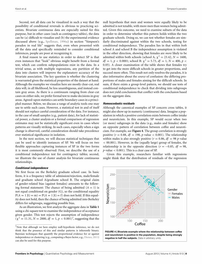
Homoscedastic residualsAlthough the canonical examples of SP concern cross tables, itmight also show up in numeric (continuous) data. Imagine a pop-ulation in which a positive correlation exists between coffee intakeand neuroticism. In this example, SP would occur when two(or more) subgroups in the data (e.g., males and females) showan opposite pattern of correlation between coffee and neuroti-cism. For example, see Figure 4. The group correlation is stronglypositive (r = 0.88, df = 198, p-value < 0.001). The relationshipwithin males is also strongly positive (r = 0.86, df = 98 p-value< 00.001). However, in the (equally large) group of females, therelationship is in the opposite direction (r = −0.85, df = 98,p-value < 0.001). This is a clear case of SP.

Given this example, researchers familiar with regressionsmight think that the distribution of residuals of the regression

FIGURE 4 | Bivariate example where the relationship between coffee

and neuroticism is positive in the population, despite being strongly

negative in half the subjects. Data in arbitrary units.

Frontiers in Psychology | Quantitative Psychology and Measurement August 2013 | Volume 4 | Article 513 | 8

Kievit et al. Simpson’s paradox

may be an informative clue of SP. A core assumption of a regres-sion model is that the residuals are homoscedastic, i.e., that thevariance of residuals is equal across the regression line (homo-geneity of variance). Inspection of Figure 4 suggests that theseresiduals are larger on the “right” side of the plot, because theregression of the females is almost orthogonal to the direction ofthe group regression. In this case, we could test for homogene-ity of residuals by means of the Breusch–Pagan test (1979) forlinear regressions. In this case, the intuition is correct: A Breusch–Pagan test rejects the assumption that residuals in Figure 4 arehomoscedastic (BP = 18.4, df = 1, p-value < 0.001). However,even homoscedastic residuals do not rule out SP. Consider theprevious example in Figure 3: Here, there are opposite patternsof correlation for each group despite equal means, variances andhomoscedastic residuals and no significant relationship at thegroup level. Fortunately, such cases are unlikely (Spirtes et al.,2000).

ClusteringCluster analysis (e.g., Kaufman and Rousseeuw, 2008) can be usedto detect the presence of subpopulations within a dataset based oncommon statistical patterns. For clarity we will restrict our dis-cussion to the bivariate case, but cluster analysis can be used withmore variables. These clusters can be described by their positionin the bivariate scatterplot (the centroid of the cluster) and thedistributional characteristics of the cluster. Recent analytic devel-opments (Friendly et al., 2013) have focused on the developmentof modeling techniques by using ellipses to quantify patterns inthe data.

In a bivariate regression, we commonly assume there is onepattern, or cluster, of data that can be described by the param-eters estimated in the regression analysis, such as the slope andintercept of the regression line. SP can occur if there exists morethan one cluster in the data: Then, the regression that describesthe group may not be the same as the regressions within clusterspresent in the data. In terms of SP, it may mean that the bivariaterelationship within the clusters might be in the opposite direc-tion of the relationship of the dataset as a whole (also known asRobinson’s paradox, 1950).

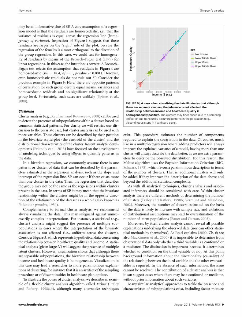
Complementary to formal cluster analysis, we recommendalways visualizing the data. This may safeguard against unnec-essarily complex interpretations. For instance, a statistical (e.g.,cluster) analysis might suggest the presence of multiple sub-populations in cases where the interpretation of the bivariateassociation is not affected (i.e., uniform across the clusters).Consider Figure 5, which represents hypothetical data concerningthe relationship between healthcare quality and income. A statis-tical analysis (given large N) will suggest the presence of multiplelatent clusters. However, visualization shows that although thereare separable subpopulations, the bivariate relationship betweenincome and healthcare quality is homogeneous. Visualization inthis case may lead a researcher to more parsimonious explana-tions of clustering, for instance that it is an artifact of the samplingprocedure or of discontinuities in healthcare plan options.

To illustrate the power of cluster analysis, we describe an exam-ple of a flexible cluster analysis algorithm called Mclust (Fraleyand Raftery, 1998a,b), although many alternative techniques

35

40

45

50

20000 30000 40000 50000 60000 70000Income ($ p.a.)

Hea

lthca

re Q

ualit

y

SES

Low income

Lower Middle Class

Upper Class

Upper Middle Class

FIGURE 5 | A case when visualizing the data illustrates that although

there are separate clusters, the inference is not affected: the

relationship between income and healthcare quality is

homogeneously positive. The clusters may have arisen due to a samplingartifact or due to naturally occurring patterns in the population (e.g.,discontinuous steps in healthcare plans).

exist. This procedure estimates the number of componentsrequired to explain the covariation in the data. Of course, muchlike in a multiple-regression where adding predictors will alwaysimprove the explained variance of a model, having more than onecluster will always describe the data better, as we use extra param-eters to describe the observed distribution. For this reason, theMclust algorithm uses the Bayesian Information Criterion (BIC,Schwarz, 1978), which favors a parsimonious description in termsof the number of clusters. That is, additional clusters will onlybe added if they improve the description of the data above andbeyond the additional statistical complexity.

As with all analytical techniques, cluster analysis and associ-ated inferences should be considered with care. Within clusteranalysis there are different methods of determining the numberof clusters (Fraley and Raftery, 1998b; Vermunt and Magidson,2002). Moreover, the number of clusters estimated on the basisof the data is likely to increase with sample size, and violationsof distributional assumptions may lead to overestimation of thenumber of latent populations (Bauer and Curran, 2003).

Moreover, by itself cluster analysis cannot reveal all possibleexplanations underlying the observed data (nor can other statis-tical methods by themselves). As Pearl explains (2000, Ch. 6; seealso MacKinnon et al., 2000) it is impossible to determine fromobservational data only whether a third variable is a confound ora mediator. The distinction is important because it determineswhether to condition on the third variable or not. At this pointbackground information about the directionality (causality) ofthe relationship between the third variable and the other two vari-ables is required. In the absence of such information, the issuecannot be resolved. The contribution of a cluster analysis is thatit can suggest cases where there may be a confound or mediator,without prior information about such variables.

Many similar analytical approaches to tackle the presence andcharacteristics of subpopulations exist, including factor mixture

www.frontiersin.org August 2013 | Volume 4 | Article 513 | 9

Kievit et al. Simpson’s paradox

models (Lubke and Muthen, 2005), latent profile models (Halpinet al., 2011) and propensity scores (Rubin, 1997). We do not nec-essarily consider cluster analysis superior to all these approachesin all respects, but implement it here for its versatility in tacklingthe current questions.

In short, analytical procedures that identify latent clusteringare no substitute for careful consideration of latent populationsthus identified: False positive identification of subgroups canunnecessarily complicate analyses and, like cases of SP, lead toincorrect inferences.

TREATMENTThe identification of the presence of clustering, specifically thepresence of more than one cluster, is a powerful and general toolin the diagnosis of a possible instance of SP. Once we have estab-lished the existence of more than one cluster, there may also bemore than one relationship between the variables of interest. Ofcourse, identification of the additional clusters is only the firststep: Next we want to “treat” the data in such a way that we canbe confident about the relationships present in the data. To do so,we have developed a tool in a freeware statistical software packagethat any interested researcher can use. Our tool can be run to (a)automatically analyze data for the presence of additional clusters,(b) run regression analyses that quantify the bivariate relationshipwithin each cluster and (c) statistically test whether the patternwithin the clusters deviates, significantly and in sign (positive ornegative) from the pattern established at the level of the aggre-gate data. In the next section, we discuss the tool, and show howit can be implemented in cases of latent clustering (estimated onthe basis of statistical characteristics as described above) or mani-fest clustering (a known and measured grouping variables such asmale and female).

A PRACTICAL APPROACH TO DETECTING SIMPSON’SPARADOXAs we have seen above, SP is interesting for a variety of concep-tual reasons: It reveals our implicit bias toward causal inference, itillustrates inferential heuristics, it is an interesting mathematicalcuriosity and forces us to carefully consider at what explana-tory level we wish to draw inferences, and whether our data aresuitable for this goal. However, in addition to these points oftheoretical interest, there is a practical element to SP: that is,what can we do to avoid or address instances of SP in a datasetbeing analyzed. Several recent approaches have aimed to tacklethis problem in various ways. One paper focuses on how to mineassociational rules from database tables that help in the iden-tification and interpretation of possible cases of SP (Froelich,2013). Another paper emphasized the importance of visualiza-tion in modeling cases of SP (Rücker and Schumacher, 2008; seealso Friendly et al., 2013). A recent approach has developed a(Java) applet (Schneiter and Symanzik, 2013) that allows users tovisualize conditional and marginal distributions for educationalpurposes. An influential account (King, 1997) of a related issue,the ecological inference problem8, has led to the development of

8“Ecological inference is the process of using aggregate (i.e., ecological) datato infer discrete individual-level relationships of interest when individual-leveldata are not available”—(King, 1997, p. xv).

various software tools (King, 2004; Imai et al., 2011; King andRoberts, 2012) to deal with proper inference from the group tothe subgroup or individual level. This latter package complementsour current approach by focusing mostly on contingency tables.The ongoing development of these various approaches illustratesthe increased recognition of the importance of identifying SPfor both substantive (novel empirical results) and educational(illustrating invalid heuristics and shortcuts) purposes.

In line with these approaches, we have developed a package,written in R (Team, 2013), a widely used, free, statistical program-ming package9. The package is freely available, can be used to aidthe detection and solution of cases of SP for bivariate continuousdata (Kievit and Epskamp, 2012), and was specifically developedto be easy to use for psychologists. The package has several bene-fits compared to the above examples. Firstly, it is written in, R, alanguage specifically tailored for a wide variety of statistical anal-yses 10. This makes it uniquely suitable for automating analysesin large datasets and integration into normal analysis pipelines,something that is be unfeasible with online applets. It special-izes in the detection of cases of Simpson’s paradox for bivariatecontinuous data with categorical grouping variables (also knownas Robinson’s paradox), a very common inference type for psy-chologists. Finally, its code is open source and can be extendedand improved upon depending on the nature of the data beingstudied. The function allows researchers to automate a search forunexpected relationships in their data. Here, we briefly describehow the function works, and apply it to two simple examples.

Imagine a dataset with some bivariate relationship of interestbetween two continuous variables X and Y. After finding, say apositive correlation, we want to check whether there might existmore than one subpopulation within the data, and test whetherthe positive correlation we found at the level for the group alsoholds for possible subpopulations. When the function is run for agiven dataset, it does three things. First, it estimates whether thereis evidence for more than one cluster in the data. Then, it esti-mates the regression of X on Y for each cluster. Finally, using apermutation test to control for dependency in the data (all clus-ters are part of the complete dataset) it examines whether therelationship within each cluster deviates significantly from thecorrelation at the level of the group (corrected for different samplesizes). If this is the case, a warning is issued as follows: “Warning:Beta regression estimate in cluster X is significantly different com-pared to the group!” If the sign of the correlation within a clusteris different (positive or negative) than the sign for the group andit deviates significantly, a warning states “Sign reversal: Simpson’sParadox! Cluster X is significantly different and in the oppositedirection compared to the group!” In this manner, a researchercan check whether whatever effect is observed in the dataset as awhole does in fact hold for possible subgroups.

For example, we might observe a bivariate relationshipbetween coffee and neuroticism. The regression suggests a

9Both the package and data examples are freely available in the CRANdatabase as Kievit and Epskamp (2012). Package “Simpsons.”10Note that the package “EI,” by King and Roberts (2012), is also written inR. EI focuses mainly on contingency tables (and on more general propertiesthan just SP), complementing our focus on continuous data.

Frontiers in Psychology | Quantitative Psychology and Measurement August 2013 | Volume 4 | Article 513 | 10

Kievit et al. Simpson’s paradox

FIGURE 6 | Using cluster analysis to uncover Simpson’s Paradox. Thecluster analysis (correctly) identifies that there are three subclusters, and thatthe relationship in two of these both deviates significantly from the groupmean, and is in the opposite direction. Data in arbitrary units.

significant positive association between coffee and neuroticism.However, when we run the SP detection algorithm a different pic-ture appears (see Figure 6). Firstly, the analysis shows that thereare three latent clusters present in our data. Secondly, we discoverthat the purported positive relationship actually only holds forone cluster: for the other two clusters, the relationship is negative.

In some cases, the researcher may have access to the rele-vant grouping variable such as “gender” or “political preference,”in which case one can easily test the homogeneity of the sta-tistical relationships at the group and subgroup level. Our toolallows for an easy way to automate this process by simply specify-ing the grouping variable, which automatically runs the bivariateregression for the whole dataset and the individual subgroups.

A final application is to identify the clusters on the basis ofdata that is not part of the bivariate association of interest. Forexample, imagine that before we analyze the relationship between“Coffee intake” and “Neuroticism,” we want to identify clus-ters (of individuals) by means of a questionnaire concerning,for example, the type of work people are in (highly stressfulor not) and how they cope with stress in a self-report ques-tionnaire. We might have reason to believe that the pattern ofassociation between coffee drinking and neuroticism is ratherdifferent depending on how people cope with stress. If so, thismight affect the group level analysis, as there may be more thanone statistical association depending on the classes of people.

Using our tool, it is possible to specify the questionnaire responsesas the data by which to cluster people. The cluster analysis ofthe questionnaire may yield, say, three clusters (types) of peo-ple in terms of how they cope with stress. We can then analyzethe relationship between coffee and neuroticism for these indi-vidual clusters and the dataset as a whole. Comparable patternshave been reported in empirical data. For instance, Reid andSullivan (2012) found such a pattern by studying the relationshipbetween being a previous crime victim and the likelihood of hav-ing offended yourself. They showed, using a latent class approachsimilar to the above example that there existed several patternsof differing (positive and negative) associations with regards tothe relationship between victimization and offense, thus pro-viding insight into the underlying causes of conflicting findingsin the literature. Such findings show complementary benefits toanalyzing data in this manner: It can help protect against incor-rect or incomplete inferences, and uncover novel relationships ofinterest.

CONCLUSIONIn this article, we have argued that SP’s status as a statisticalcuriosity is unwarranted, and that SP deserves explicit consid-eration in psychological science. In addition, we expanded thenotion of SP from traditional cross-table counts to include a rangeof other research designs, such as intra-individual measurementsover time (across development or experimental time scales), andstatistical techniques, such as bivariate continuous relationships.Moreover, we discussed existing studies showing that, unlessexplicitly primed to consider conditional and marginal probabil-ities, people are generally not adept at recognizing possible casesof SP.

To adequately address SP, a variety of inferential and practi-cal strategies can be employed. Research designs can incorporatedata collection that facilitates the comparison of patterns acrossexplanatory levels. Researchers should carefully examine, ratherthan assume that relationships at the group level also hold for sub-groups or individuals over time. To this end, we have developed atool to facilitate the detection of hitherto undetected patterns ofassociation in existing datasets.

An appreciation of SP provides an additional incentive to care-fully consider the precise fit between the research questions weask, the designs we develop, and the data we obtain. Simpson’sparadox is not a rare statistical curiosity, but a striking illustra-tion of our inferential blind spots, and a possible avenue into arange of novel and exciting findings in psychological science.

REFERENCESAldrich, J. (1995). Correlations genuine

and spurious in Pearson and Yule.Stat. Sci. 10, 364–376.

Anderson, K. J., Revelle, W., and Lynch,M. J. (1989). Caffeine, impulsivity,and memory scanning: a com-parison of two explanations forthe Yerkes-Dodson Effect. Motiv.Emot. 13, 1–20. doi: 10.1007/BF00995541

Bandyoapdhyay, P. S., Nelson, D.,Greenwood, M., Brittan, G., and

Berwald, J. (2011). The logic ofSimpson’s paradox. Synthese 181,185–208. doi: 10.1007/s11229-010-9797-0

Batty, G. D., Deary, I. J., Schoon, I.,Emslie, C., Hunt, K., and Gale,C. R. (2008). Childhood men-tal ability and adult alcoholintake and alcohol prob-lems: the 1970 British CohortStudy. Am. J. Public Health 98,2237–2243. doi: 10.2105/AJPH.2007.109488

Bauer, D. B., and Curran, P. J. (2003).Distributional assumptions ofgrowth mixture models: implica-tions for overextraction of latenttrajectory classes. Psychol. Methods8, 338–363. doi: 10.1037/1082-989X.8.3.338

Benjamin, L. T., Cavell, T. A., andShallenberger, W. R. (1987).“Staying with initial answers onobjective tests: is it a myth?,” inHandbook on Student Development:Advising, Career Development,

and Field Placement, eds M.E. Ware, and R. J. Millard(Hillsdale, NJ: Lawrence Erlbaum),45–53.

Bickel, P. R., Hammel, E. A., andO’Connell, J. W. (1975). Sexbias in graduate admissions:data from Berkeley. Science 187,398–404.

Block, N. (1995). How heritabilitymisleads about race. Cognition 56,99–128. doi: 10.1016/0010-0277(95)00678-R

www.frontiersin.org August 2013 | Volume 4 | Article 513 | 11

Kievit et al. Simpson’s paradox

Blyth, C. R. (1972). On Simpson’sparadox and the sure-thing prin-ciple. J. Am. Statist. Assoc. 67,364–366. doi: 10.1080/01621459.1972.10482387

Borsboom, D., Kievit, R. A., Cervone,D. P., and Hood, S. B. (2009).“The two disciplines of scientificpsychology, or: the disunity of psy-chology as a working hypothesis,” inDevelopmental Process Methodologyin the Social and DevelopmentalSciences, eds J. Valsiner, P. C. M.Molenaar, M. C. D. P. Lyra, andN. Chaudary (New York, NY:Springer), 67–89.

Breusch, T. S., and Pagan, A. R. (1979).Simple test for heteroscedasticityand random coefficient variation.Econometrica 47, 1287–1294. doi:10.2307/1911963

Cartwright, N. (1979). Causallaws and effective strategies.Nous 13, 419–437. doi: 10.2307/2215337

Cattell, R. B. (1952). The three basicfactor-analytic research designs-their interrelations and derivatives.Psychol. Bull. 49, 499–520. doi:10.1037/h0054245

Chater, N., Vlaev, I., and Grinberg,M. (2008). A new consequence ofSimpson’s paradox: stable coopera-tion in one-shot prisoner’s dilemmafrom populations of individualis-tic learners. J. Exp. Psychol. Gen.137, 403–421. doi: 10.1037/0096-3445.137.3.403

Chuang, J. S., Rivoire, O., and Leibler,S. (2009). Simpson’s paradox in asynthetic microbial system. Science323, 272–275. doi: 10.1126/science.1166739

Cohen, M. R., and Nagel, E. (1934). AnIntroduction to Logic and ScientificMethod. New York, NY: Harcourt,Brace and Company.

Conger, A. J. (1974). A revised def-inition for suppressor variables:a guide to their identificationand interpretation. Educ. Psychol.Meas. 34, 35–46. doi: 10.1177/001316447403400105

Curley, S. P., and Browne, G. J.(2001). Normative and descrip-tive analyses of Simpson’s para-dox in decision making. Organ.Behav. Hum. Decis. Process. 84,308–333. doi: 10.1006/obhd.2000.2928

Dawid, A. P. (1979). Conditional inde-pendence in statistical theory. J. Roy.Stat. Soc. Ser. B (Methodol.) 41,1–31.

Dienes, Z. (2011). Bayesian versusorthodox statistics: which sideare you on? Perspect. Psychol.Sci. 6, 274–290. doi: 10.1177/1745691611406920

Dutilh, G., Wagenmakers, E. J.,Visser, I., and van der Maas, H.L. (2011). A phase transitionmodel for the speed-accuracytrade−off in response timeexperiments. Cogn. Sci. 35,211–250. doi: 10.1111/j.1551-6709.2010.01147.x

Fiedler, K. (2000). Beware of sam-ples!: a cognitive–ecologicalsampling approach to judg-ment biases. Psychol. Rev. 107,659–676. doi: 10.1037/0033-295X.107.4.659

Fiedler, K. (2008). The ultimate sam-pling dilemma in experience-based decision making. J. Exp.Psychol. Learn. Mem. Cogn. 34,186–203. doi: 10.1037/0278-7393.34.1.186

Fiedler, K., Freytag, P., and Meisder,T. (2009). Pseudocontingencies: anintegrative account of an intrigu-ing cognitive illusion. Psychol.Rev. 116,187–206. doi: 10.1037/a0014480

Fiedler, K., Walther, E., Freytag, P.,and Nickel, S. (2003). Inductive rea-soning and judgment interference:experiments on Simpson’s para-dox. Pers. Soc. Psychol. Bull. 29,14–27. doi: 10.1177/0146167202238368

Fisher, R. A. (1925). Statistical Methodsfor Research Workers. Edinburgh:Oliver and Boyd.

Fitts, P. M. (1954). The informa-tion capacity of the human motorsystem in controlling the ampli-tude of movement. J. Exp. Psychol.47, 381–391. doi: 10.1037/h0055392

Fraley, C., and Raftery, A. E. (1998a).MCLUST: Software for Model-BasedCluster and Discriminant Analysis.Department of Statistics, Universityof Washington: Technical ReportNo. 342.

Fraley, C., and Raftery, A. E. (1998b).How many clusters? Which cluster-ing method? Answers via model-based cluster analysis. Comput J. 41,578–588.

Friendly, M., Monette, G., and Fox,J. (2013). Elliptical insights:understanding statistical methodsthrough elliptical geometry. Stat.Sci. 28(1), 1–39. doi: 10.1214/12-STS402

Froelich, W. (2013). “Mining associ-ation rules from database tableswith the instances of Simpson’sparadox,” in Advances in Databasesand Information Systems, eds M.Tadeusz, H. Theo, and W. Robert(Berlin; Heidelberg: Springer),79–90.

Greenland, G. (2010). Simpson’s para-dox from adding constants in con-tingency tables as an example of

bayesian noncollapsibility. Am. Stat.64, 340–344. doi: 10.1198/tast.2010.10006

Halpin, P. F., Dolan, C. V., Grasman,R. P., and De Boeck, P. (2011).On the relation between the lin-ear factor model and the latentprofile model. Psychometrika 76,564–583. doi: 10.1007/s11336-011-9230-8

Hamaker, E. L., Nesselroade, J. R., andMolenaar, P. C. M. (2007). The inte-grated trait- state model. J. Res. Pers.41, 295–315. doi: 10.1016/j.jrp.2006.04.003

Hernán, M. A., Clayton, D., andKeiding, N. (2011). The Simpson’sparadox unraveled. Int. J. Epidemiol.40, 780–785. doi: 10.1093/ije/dyr041

Herrnstein, R. J., and Murray, C.(1994). Bell curve: Intelligence andclass structure in American life.(New York, NY: Free Press).

Hintzman, D. L. (1980). Simpson’sparadox and the analysis of mem-ory retrieval. Psychol. Rev. 87,398–410. doi: 10.1037/0033-295X.87.4.398

Hintzman, D. L. (1993) On variabil-ity, Simpson’s paradox, and the rela-tion between recognition and recall:reply to Tulving and Flexser. Psychol.Rev. 100, 143–148.

Imai, K., Lu, Y., and Strauss, A. (2011).Eco: R package for ecological infer-ence in 2x2 tables. J. Stat. Softw. 42,1–23.

Jensen, A. R. (1998). The g Factor: TheScience of Mental Ability. Westport,CT: Praeger.

Julious, S. A., and Mullee, M. A. (1994).Confounding and Simpson’s para-dox. Br. Med. J. 209, 1480–1481. doi:10.1136/bmj.309.6967.1480

Kanazawa, S. (2010). Evolutionary psy-chology and intelligence research.Am. Psychol. 65, 279–289. doi:10.1037/a0019378

Kaufman, L., and Rousseeuw, P. J.(2008) Introduction, in FindingGroups in Data: An Introduction toCluster Analysis. Hoboken, NJ: JohnWiley and Sons, Inc.

Kievit, R. A., and Epskamp, S. (2012).Simpsons: Detecting Simpson’sParadox. R package version 0.1.0.Available online at: http://CRAN.

R-project.org/package=SimpsonsKievit, R. A., Romeijn, J. W., Waldorp,

L. J., Scholte, H. S., Wicherts, J.M., and Borsboom, D. (2011). Mindthe gap: a psychometric approach tothe reduction problem. Psychol. Inq.22, 67–87. doi: 10.1080/1047840X.2011.550181

Kievit, R. A., van Rooijen, H., Wicherts,J. M., Waldorp, L. J., Kan, K.J., Scholte, H. S., et al. (2012a).

Intelligence and the brain: a model-based approach. Cogn. Neurosci. 3,89–97. doi: 10.1080/17588928.2011.628383

Kievit, R. A., Waldorp, L. J., Kan, K.J., and Wicherts, J. M. (2012b).Causality: populations, individuals,and assumptions. Eur. J. Pers. 26,400–401.

King, G. (1997). A Solution to theEcological Inference Problem:Reconstructing Individual Behaviorfrom Aggregate Data. Princeton:Princeton University Press.

King, G. (2004). EI: a program for eco-logical inference. J. Stat. Softw. 11,1–38.

King, G., and Roberts, M. (2012).EI: a (n R) program for eco-logical inference. 1–27. Availableonline at: http://gking.harvard.edu/files/gking/files/ei.pdf

Kraemer, H. C., Wilson, K. A.,and Hayward, C. (2006).Lifetime prevalence and pseu-docomorbidity in psychiatricresearch. Arch. Gen. Psychiatry 63,604–608. doi: 10.1001/archpsyc.63.6.604

Kramer, G. H. (1983). The ecologicalfallacy revisited: aggregate-versusindividual-level findings oneconomics and elections, andsociotropic voting. Am. Polit. Sci.Rev. 77, 92–111. doi: 10.2307/1956013

Lewontin, R. C. (2006). The analysis ofvariance and the analysis of causes.Int. J. Epidemiol. 35, 520–525. doi:10.1093/ije/dyl062

Loftus, G. R. (1993). A picture isworth a thousand p values: on theirrelevance of hypothesis testingin the microcomputer age. Behav.Res. Methods Instrum. Comput.25, 250–256. doi: 10.3758/BF03204506

Lubke, G. H., and Muthen, B. (2005).Investigating population het-erogeneity with factor mixturemodels. Psychol. Methods 10,21–39. doi: 10.1037/1082-989X.10.1.21

MacKay, D. G. (1982). The prob-lems of flexibility, fluency, andspeed–accuracy trade-off inskilled behavior. Psychol. Rev. 89,483–506. doi: 10.1037/0033-295X.89.5.483

MacKinnon, D. P., Fairchild, A. J.,and Fritz, M. S. (2007). Mediationanalysis. Annu. Rev. Psychol.58, 593.

MacKinnon, D. P., Krull, J. L.,and Lockwood, C. M. (2000).Equivalence of the mediation, con-founding and suppression effect.Prev. Sci. 1, 173–181. doi: 10.1023/A:1026595011371

Frontiers in Psychology | Quantitative Psychology and Measurement August 2013 | Volume 4 | Article 513 | 12

Kievit et al. Simpson’s paradox

Martin, E. (1981). Simpson’sparadox resolved: a reply toHintzman. Psychol. Rev. 88,372–374. doi: 10.1037/0033-295X.88.4.372

Mazur, A., and Booth, A. (1998).Testosterone and dominancein men. Behav. Brain Sci. 21,353–397. doi: 10.1017/S0140525X98001228

McCrae, R. R., and Costa, P. T. (2008).“Empirical and theoretical sta-tus of the five-factor model ofpersonality traits,” in The SAGEHandbook of Personality Theoryand Assessment, Vol. 1: PersonalityTheories and Models, eds G. J. Boyle,G. Matthews, and D. H. Saklofske(London: SAGE publishers),273–294. doi: 10.4135/9781849200462.n13

McCrae, R. R., and John, O. P. (1992).An introduction to the five-factormodel and its applications. J. Pers.60, 175–215. doi: 10.1111/j.1467-6494.1992.tb00970.x

Miller, G. (2012). The smartphone psy-chology manifesto. Perspect. Psychol.Sci. 7, 221–237.

Molenaar, P. C. M. (2004). A mani-festo on psychology as idiographicscience: bringing the person backinto scientific psychology, thistime forever. Measurement 2,201–218.

Molenaar, P. C. M., and Campbell,C. G. (2009). The new person-specific paradigm in psychology.Curr. Dir. Psychol. Sci. 18,112–117. doi: 10.1111/j.1467-8721.2009.01619.x

Molenaar, P. C. M., Huizenga, H.M., and Nesselroade, J. R. (2003).“The relationship between thestructure of inter–individual andintra–individual variability: atheoretical and empirical vindi-cation of developmental systemstheory,” in Understanding HumanDevelopment: Dialogues withLifespan Psychology, eds U. M.Staudinger and U. Lindenberger(Boston: Kluwer AcademicPublishers), 339–360).

Na, J., Grossmann, I., Varnum,M. E., Kitayama, S., Gonzalez,R., and Nisbett, R. E. (2010).Cultural differences are not alwaysreducible to individual differences.Proc. Natl. Acad. Sci. U.S.A. 107,6192–6197. doi: 10.1073/pnas.1001911107

Otte, R. (1985). Probabilistic causal-ity and Simpson’s Paradox. Philos.Sci. 52, 110–125. doi: 10.1086/289225

Pavlides, M. G., and Perlman, M. D.(2009). How likely is Simpson’sparadox? Am. Stat. 63, 226–233.

Pearl, J. (1999). Simpson’s Paradox: AnAnatomy. UCLA Cognitive SystemsLaboratory, Technical Report.

Pearl, J. (2000). Causality: Models,Reasoning and Inference.Cambridge: Cambridge UniversityPress.

Pearl, J. (2013). Linear models: auseful “microscope” for causalanalysis. J. Causal Inference 1,155–170.

Pearson, K., Lee, A., and Bramley-Moore, L. (1899). Genetic repro-ductive selection: inheritance of fer-tility in man. Philos. Trans. R. Soc. A.192, 257–330.

Penke, L., Johnson, W., Kievit, R. A.,Wicherts, J. M., Ploeger, A., andBorsboom, D. (2011). Evolutionarypsychology and intelligence researchcannot be integrated the wayKanazawa (2010) suggests. Am.Psychol. 66, 916–917. doi: 10.1037/a0024626

Reid, J. A., and Sullivan, C. J. (2012).Unraveling victim-offender overlap:exploring profiles and constella-tions of risk. Vict. Offenders. 7,327–360. doi: 10.1080/15564886.2012.685216

Robinson, W. S. (1950). Ecologicalcorrelations and the behav-ior of individuals. Am. Sociol.Rev. 15, 351–357. doi: 10.2307/2087176

Rosenbaum, P. R., and Rubin, D. B.(1983). The central role of thepropensity score in observationalstudies for causal effects. Biometrika70, 41–55. doi: 10.1093/biomet/70.1.41

Rubin, D. B. (1997). Estimating causaleffects from large data sets usingpropensity scores. Ann. Intern. Med.127, 757–763. doi: 10.7326/0003-4819-127-8_Part_2-199710151-00064

Rubin, D. R. (2011). An alternativeto pooling Kaplan-Meier curves intime-to-event meta-analysis. Int. J.Biostat. 7, 1–26. doi: 10.2202/1557-4679.1289

Rücker, G., and Schumacher, M.(2008). Simpson’s paradoxvisualized: the example of therosiglitazone meta-analysis. BMCMed. Res. Methodol. 8:34. doi:10.1186/1471-2288-8-34

Schaller, M. (1992). Sample size, aggre-gation, and statistical reasoning insocial inference. J. Exp. Soc. Psychol.28, 65–85. doi: 10.1016/0022-1031(92)90032-F

Scheiner, S. M., Cox, S. B., Willig,M., Mittelbach, G. G., Osenberg,C., and Kaspari, M. (2000). Speciesrichness, species–area curves andSimpson’s paradox. Evol. Ecol. Res. 2,791–802.

Schield, M. (1999). Simpson’sparadox and Cornfield’s condi-tions. ASA Proc. Sect. Stat. Educ.106–111.

Schneiter, K., and Symanzik, J. (2013).J. Stat. Educ. 21, 1–20.

Schwarz, G. (1978). Estimating thedimension of a model. Ann. Stat.6, 461–464. doi: 10.1214/aos/1176344136

Shaw, P., Greenstein, D., Lerch, J.,Clasen, L., Lenroot, R., Gogtay,N., et al. (2006). Intellectual abil-ity and cortical development inchildren and adolescents. Nature440, 676–679. doi: 10.1038/nature04513

Shweder, R. (1973). The between andwithin of cross-cultural research.Ethos 1, 531–545. doi: 10.1525/eth.1973.1.4.02a00150

Simpson, E. H. (1951). The interpre-tation of interaction in contingencytables. J. R. Stat. Soc. Ser. B 13,238–241.

Spellman, B. A. (1996a). Acting as intu-itive scientists: contingency judg-ments are made while control-ling for alternative potential causes.Psychol. Sci. 7, 337–334.

Spellman, B. A. (1996b). Conditioningcausality. Psychol. Learn. Motiv. 34,167–206.

Spellman, B. A., Price, C. M., andLogan, J. (2001). How two causesare different from one: the useof (un)conditional informationin Simpson’s paradox. Mem.Cogn. 29, 193–208. doi: 10.3758/BF03194913

Spirtes, P., Glymour, C., and Scheines,R. (2000). Causation, prediction,and search (Vol. 81). The MITPress.

Suh, G. H. (2009). The use of atyp-ical antipsychotics in dementia:rethinking Simpson’s para-dox. Int. Psychogeriatr. 21,616–621. doi: 10.1017/S1041610209008485

Tamnes, C. K., Fjell, A. M., Østby,Y., Westlye, L. T., Due-Tønnessen,P., Bjørnerud, A., et al. (2011).The brain dynamics of intellec-tual development: waxing andwaning white and gray matter.Neuropsychologia 49, 3605–3611.doi: 10.1016/j.neuropsychologia.2011.09.012

Team, R. D. C. (2013). R: A Languageand Environment for StatisticalComputing. Vienna, Austria:R Foundation for StatisticalComputing.

Tu, Y. K., Gunnell, D. J., and Gilthorpe,M. S. (2008). Simpson’s paradox,Lord’s paradox, and suppressioneffects are the same phenomenon—the reversal paradox. Emerg. Themes

Epidemiol. 5, 2. doi: 10.1186/1742-7622-5-2

Tzambazis, K., and Stough, C. (2000).Alcohol impairs speed of infor-mation processing and simpleand choice reaction time and dif-ferentially impairs higher-ordercognitive abilities. Alcohol Alcohol.35, 197–201. doi: 10.1093/alcalc/35.2.197

van der Linden, W. J., Jeon, M., andFerrara, S. (2011). A paradox inthe study of the benefits of test-item review. J. Educ. Meas. 48,380–398. doi: 10.1111/j.1745-3984.2011.00151.x

Van Rijn, P. (2008). CategoricalTime Series in PsychologicalMeasurement. University ofAmsterdam, Unpublished doctoraldissertation.

Vermunt, J. K., and Magidson, J.(2002). “Latent class cluster anal-ysis,” in Applied Latent ClassAnalysis, eds J. A. Hagenaars andA. L. McCutcheon (Cambridge,UK: Cambridge University Press),89–106.

Wagner, C. H. (1982). Simpson’s para-dox in real life. Am. Stat. 36, 46–48.

Wainer, H. (1986). Minority contribu-tions to the SAT score turnaround:an example of Simpson’s paradox.J. Educ. Behav. Stat. 11, 239–244.doi: 10.3102/10769986011004239

Waldmann, M. R., and Hagmayer,Y. (1995). “When a cause simul-taneously produces and preventsan effect,” in Proceedings of theSeventeenth Annual Conference ofthe Cognitive Science Society, J. D.Moore and J. F. Lehman (Hillsdale,NJ: Erlbaum), 425–430.

Wardrop, R. L. (1995). Simpson’s para-dox and the hot hand in basketball.Am. Stat. 49, 24–28.

Wicherts, J. M., Bakker, M., andMolenaar, D. (2011). Willingness toshare research data is related tothe strength of the evidence andthe quality of reporting of statisti-cal results. PLoS ONE 6:e26828. doi:10.1371/journal.pone.0026828

Wicherts, J. M., Borsboom, D., Kats, J.,and Molenaar, D. (2006). The pooravailability of psychological researchdata for reanalysis. Am. Psychol. 61,726–728. doi: 10.1037/0003-066X.61.7.726

Wickham, H. (2009). ggplot2: ElegantGraphics for Data Analysis. SpringerPublishing Company, Incorporated.

Wilmoth, D. R. (2012). Intelligenceand past use of recreational drugs.Intelligence 40, 15–22.

Yaari, G., and Eisenmann, S. (2011).The hot (invisible?) hand: can timesequence patterns of success/failurein sports be modeled as repeated

www.frontiersin.org August 2013 | Volume 4 | Article 513 | 13

Kievit et al. Simpson’s paradox

random independent trials? PLoSONE 6:e24532. doi: 10.1371/journal.pone.0024532

Yule, G. U. (1903). Notes on the theoryof association of attributes in statis-tics. Biometrika 2, 121–134. doi:10.1093/biomet/2.2.121

Conflict of Interest Statement: Theauthors declare that the research

was conducted in the absence of anycommercial or financial relationshipsthat could be construed as a potentialconflict of interest.

Received: 04 May 2013; accepted: 19 July2013; published online: 12 August 2013.Citation: Kievit RA, Frankenhuis WE,Waldorp LJ and Borsboom D (2013)

Simpson’s paradox in psychological sci-ence: a practical guide. Front. Psychol.4:513. doi: 10.3389/fpsyg.2013.00513This article was submitted to Frontiersin Quantitative Psychology andMeasurement, a specialty of Frontiers inPsychology.Copyright © 2013 Kievit, Frankenhuis,Waldorp and Borsboom. This is an open-access article distributed under the terms

of the Creative Commons AttributionLicense (CC BY). The use, distribution orreproduction in other forums is permit-ted, provided the original author(s) orlicensor are credited and that the origi-nal publication in this journal is cited, inaccordance with accepted academic prac-tice. No use, distribution or reproductionis permitted which does not comply withthese terms.

Frontiers in Psychology | Quantitative Psychology and Measurement August 2013 | Volume 4 | Article 513 | 14